Shape-aware Deep Convolutional Neural Network for...
12
Shape-aware Deep Convolutional Neural Network for Vertebrae Segmentation S M Masudur Rahman Al Arif 1 , Karen Knapp 2 and Greg Slabaugh 1 1 City, University of London 2 University of Exeter Abstract. Shape is an important characteristic of an object, and fundamental topic in computer vision. In image segmentation, shape has been widely used in segmentation methods, like the active shape model, to constrain a segmentation result to a class of learned shapes. However, to date, shape has been underutilised in deep segmentation networks. This paper addresses this gap by introducing a shape-aware term in the segmentation loss function. A deep convolutional net- work has been adapted in a novel cervical vertebrae segmentation framework and compared with traditional active shape model based methods. The proposed framework has been trained on an augmented dataset of 26370 vertebrae and tested on 792 vertebrae collected from a total of 296 real-life emergency room lateral cervical X-ray images. The proposed framework achieved an average er- ror of 1.11 pixels, signifying a 36% improvement over the traditional methods. The introduction of the novel shape-aware term in the loss function significantly improved the performance by further 12%, achieving an average error of only 0.99 pixel. 1 Introduction Deep learning has revolutionized the field of image classification [1–4], segmenta- tion [5–7] and many other aspects of computer vision. Segmenting an anatomical body part in medical images is a challenging problem in the field. Although, training a deep network requires huge amount of data, which is usually not available for medical im- ages, recent techniques using data augmentation have shown promising results for seg- mentation problem on medical images [8, 9]. Shape characteristics have long been used for image segmentation problems, especially in medical images [10–13]. Medical im- age modalities, e.g. X-ray, DXA, MRI, often produce noisy captures of anatomical body parts, where segmentation must rely on the shape information to produce reliable results. However, combining shape information in a deep segmentation network is not straightforward. In this paper, we try to solve the problem by introducing a novel shape- aware term in the segmentation loss function. To test its capability of shape preserva- tion, we adapted the novel shape-aware deep segmentation network in a semi-automatic cervical vertebrae segmentation framework. Segmenting the vertebrae correctly is a crucial part for further analysis in an injury detection system. Previous work in vertebrae segmentation has largely been dominated
Transcript of Shape-aware Deep Convolutional Neural Network for...
Shape-aware Deep Convolutional Neural Network forVertebrae Segmentation
S M Masudur Rahman Al Arif1, Karen Knapp2 and Greg Slabaugh1
1City, University of London2University of Exeter
Abstract. Shape is an important characteristic of an object, and fundamentaltopic in computer vision. In image segmentation, shape has been widely used insegmentation methods, like the active shape model, to constrain a segmentationresult to a class of learned shapes. However, to date, shape has been underutilisedin deep segmentation networks. This paper addresses this gap by introducing ashape-aware term in the segmentation loss function. A deep convolutional net-work has been adapted in a novel cervical vertebrae segmentation frameworkand compared with traditional active shape model based methods. The proposedframework has been trained on an augmented dataset of 26370 vertebrae andtested on 792 vertebrae collected from a total of 296 real-life emergency roomlateral cervical X-ray images. The proposed framework achieved an average er-ror of 1.11 pixels, signifying a 36% improvement over the traditional methods.The introduction of the novel shape-aware term in the loss function significantlyimproved the performance by further 12%, achieving an average error of only0.99 pixel.
1 Introduction
Deep learning has revolutionized the field of image classification [1–4], segmenta-tion [5–7] and many other aspects of computer vision. Segmenting an anatomical bodypart in medical images is a challenging problem in the field. Although, training a deepnetwork requires huge amount of data, which is usually not available for medical im-ages, recent techniques using data augmentation have shown promising results for seg-mentation problem on medical images [8,9]. Shape characteristics have long been usedfor image segmentation problems, especially in medical images [10–13]. Medical im-age modalities, e.g. X-ray, DXA, MRI, often produce noisy captures of anatomicalbody parts, where segmentation must rely on the shape information to produce reliableresults. However, combining shape information in a deep segmentation network is notstraightforward. In this paper, we try to solve the problem by introducing a novel shape-aware term in the segmentation loss function. To test its capability of shape preserva-tion, we adapted the novel shape-aware deep segmentation network in a semi-automaticcervical vertebrae segmentation framework.
Segmenting the vertebrae correctly is a crucial part for further analysis in an injurydetection system. Previous work in vertebrae segmentation has largely been dominated
by statistical shape model (SSM) based approaches [14–22]. These methods record sta-tistical information about the shape and/or the appearance of the vertebrae based on atraining set. Then the mean shape is initialized either manually or semi-automaticallynear the actual vertebra. The model then tries to converge to the actual vertebra bound-ary based on a search procedure. Recent work, [19–22] utilizes random forest basedmachine learning models in order to achieve shape convergence. In contrast to thesemethods, we propose a novel deep convolutional neural network (CNN) based methodfor vertbrae segmentation. Instead of predicting the shape of a vertebra, our frameworkpredicts the segmentation mask of a vertebrae patch. In order to preserve the vertebrashape, a novel shape-aware loss term has been proposed. From a training set of 124X-ray images containing 586 cervical vertebrae, 26370 vertebrae patch-segmentationmask pairs have been generated through data augmentation for training the deep net-work. The trained framework has been tested on dataset of 172 images containing792 vertebrae. An average pixel-level accuracy of 97.01%, Dice similarity coefficient0.9438 and shape error of 0.99 pixel have been achieved.
The key contributions of this work are two fold. First, the introduction of a novelshape-aware term in the loss function of a deep segmentation network which learnsto preserve the shape of the target object and significantly improved the segmenta-tion accuracy. Second, the application and adaptation of deep segmentation networksto achieve vertebrae segmentation in real life medical images which outperformed thetraditional SSM based methods by 35%.
2 Data
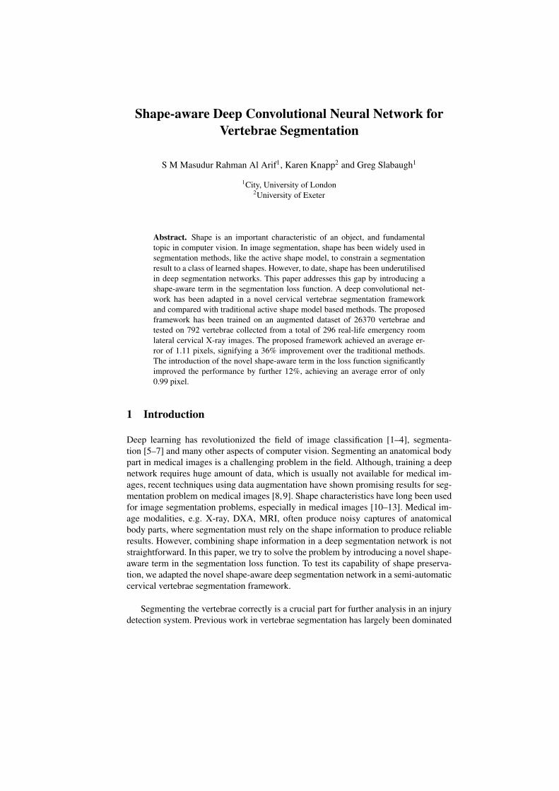
A total of 296 lateral cervical spine X-ray images were collected from Royal Devonand Exeter Hospital in association with the University of Exeter. The age of the patientsvaried from 17 to 96. Different radiographic systems (Philips, Agfa, Kodak, GE) wereused to produce the scans. Image resolution varied from 0.1 to 0.194 mm per pixel. Theimages include examples of vertebrae with fractures, degenerative changes and boneimplants. The data is anonymized and standard research protocols have been followed.The size, shape, orientation of spine, image intensity, contrast, noise level all variedgreatly in the dataset. For this work, 5 vertebrae C3-C7 are considered. C1 and C2 havean ambiguous appearance due to their ovelap in lateral cervical radiographs, and ourclinical experts were not able to provide ground truth segmentations for these vertebal
Fig. 1: X-Ray images and manual annotations. Center: blue plus (+) Vertebrae boundary curve(green).
bodies. For this reason they are excluded in this study, similar to other cervical spineimage analysis research [15, 23]. Each vertebra from the images was manually anno-tated for the vertebral body boundaries and centers by an expert radiographer. A fewexamples with corresponding manual annotations are shown in Fig. 1.
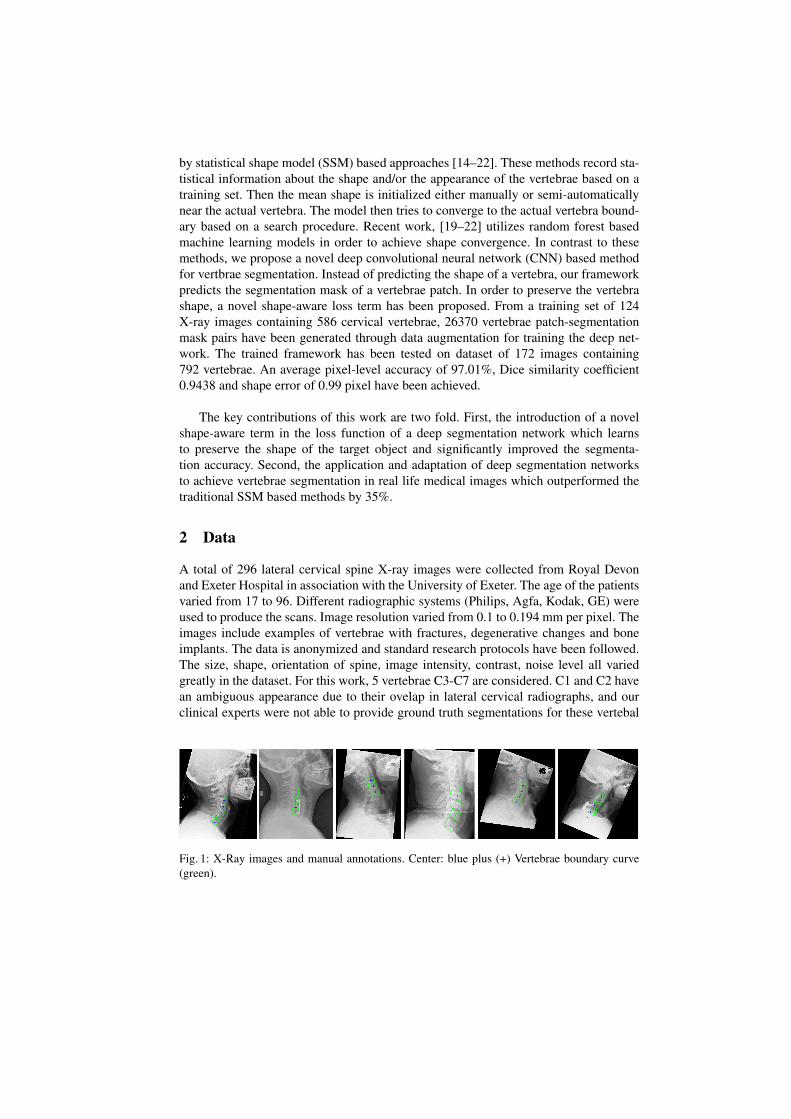
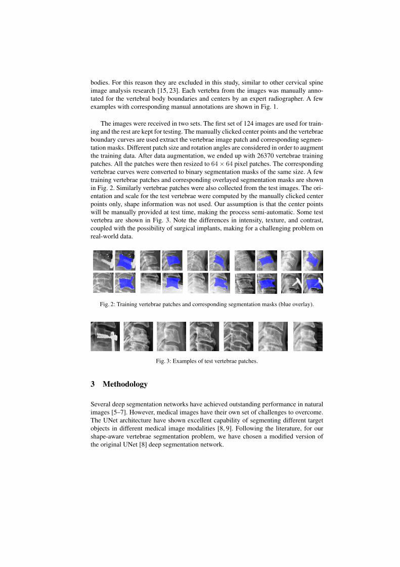
The images were received in two sets. The first set of 124 images are used for train-ing and the rest are kept for testing. The manually clicked center points and the vertebraeboundary curves are used extract the vertebrae image patch and corresponding segmen-tation masks. Different patch size and rotation angles are considered in order to augmentthe training data. After data augmentation, we ended up with 26370 vertebrae trainingpatches. All the patches were then resized to 64× 64 pixel patches. The correspondingvertebrae curves were converted to binary segmentation masks of the same size. A fewtraining vertebrae patches and corresponding overlayed segmentation masks are shownin Fig. 2. Similarly vertebrae patches were also collected from the test images. The ori-entation and scale for the test vertebrae were computed by the manually clicked centerpoints only, shape information was not used. Our assumption is that the center pointswill be manually provided at test time, making the process semi-automatic. Some testvertebra are shown in Fig. 3. Note the differences in intensity, texture, and contrast,coupled with the possibility of surgical implants, making for a challenging problem onreal-world data.
Fig. 2: Training vertebrae patches and corresponding segmentation masks (blue overlay).
Fig. 3: Examples of test vertebrae patches.
3 Methodology
Several deep segmentation networks have achieved outstanding performance in naturalimages [5–7]. However, medical images have their own set of challenges to overcome.The UNet architecture have shown excellent capability of segmenting different targetobjects in different medical image modalities [8, 9]. Following the literature, for ourshape-aware vertebrae segmentation problem, we have chosen a modified version ofthe original UNet [8] deep segmentation network.
3.1 Network architecture
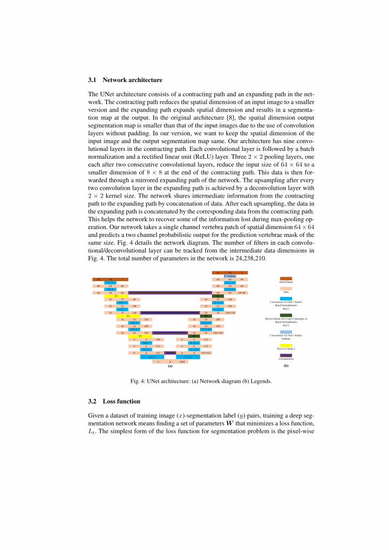
The UNet architecture consists of a contracting path and an expanding path in the net-work. The contracting path reduces the spatial dimension of an input image to a smallerversion and the expanding path expands spatial dimension and results in a segmenta-tion map at the output. In the original architecture [8], the spatial dimension outputsegmentation map is smaller than that of the input images due to the use of convolutionlayers without padding. In our version, we want to keep the spatial dimension of theinput image and the output segmentation map same. Our architecture has nine convo-lutional layers in the contracting path. Each convolutional layer is followed by a batchnormalization and a rectified linear unit (ReLU) layer. Three 2× 2 pooling layers, oneeach after two consecutive convolutional layers, reduce the input size of 64 × 64 to asmaller dimension of 8 × 8 at the end of the contracting path. This data is then for-warded through a mirrored expanding path of the network. The upsampling after everytwo convolution layer in the expanding path is achieved by a deconvolution layer with2 × 2 kernel size. The network shares intermediate information from the contractingpath to the expanding path by concatenation of data. After each upsampling, the data inthe expanding path is concatenated by the corresponding data from the contracting path.This helps the network to recover some of the information lost during max-pooling op-eration. Our network takes a single channel vertebra patch of spatial dimension 64×64and predicts a two channel probabilistic output for the prediction vertebrae mask of thesame size. Fig. 4 details the network diagram. The number of filters in each convolu-tional/deconvolutional layer can be tracked from the intermediate data dimensions inFig. 4. The total number of parameters in the network is 24,238,210.
64 64 2
fC-Softmax
64 64 1 64 64 64
C1_1 C_1_1
64 64 64 64 64 64
C1_2 C_1_2
64 64 64 64 64 64+64
D1
32 32 64 32 32 128
C2_1 C_2_1
32 32 128 32 32 128
C2_2 C_2_2
32 32 128 32 32 128+128
D2
16 16 128 16 16 256
C3_1 C_3_1
16 16 256 16 16 256
C3_2 C_3_2
16 16 256 16 16 256+256
D3
8 8 256 8 8 512
C4_1 C_4_1
8 8 512 8 8 512
C4_2 C_4_2
8 8 512 8 8 512+512
8 8 1024
(a)
Input/Output
Data
Convolution 3x3 Pad 1 Stride1
Batch Normalization
ReLU
Deconvolution 2x2 Crop 0 Upsample x2
Batch Normalization
ReLU
Convolution 3x3 Pad 1 Stride1
Softmax
Pool 2x2 Stride 2
Concatenation
(b)
C5_1
P3
P2
P1
C_5_1
Fig. 4: UNet architecture: (a) Network diagram (b) Legends.
3.2 Loss function
Given a dataset of training image (x)-segmentation label (y) pairs, training a deep seg-mentation network means finding a set of parameters W that minimizes a loss function,Lt. The simplest form of the loss function for segmentation problem is the pixel-wise
log loss.
W = argminW
N∑n=1
Lt(x(n), y(n);W ) (1)
where N is the number of training examples and x(n), y(n) represents n-th examplein the training set with corresponding manual segmentation. The pixel-wise segmenta-tion loss per image can be defined as:
Lt(x, y;W ) = −∑iεΩp
M∑j=1
yji logP (yji = 1|xi;W ) (2)
P (yji = 1|xi;W ) =exp(aj(xi))∑Mk=1 exp(ak(xi))
(3)
where aj(xi) is the output of the penultimate activation layer of the network for thepixel xi, Ωp represents the pixel space, M is the total number of segmentation classlabels and P are the corresponding class probabilities. However, this term doesn’tconstrain the predicted masks to conform to possible vertebra shapes. Since verte-brae shapes are known from the provided manual segmentation curves, we add a novelshape-aware term in the loss function to force the network to learn to penalize predictedareas outside the curve.
3.3 Shape-aware term
For training the deep segmentation network, we introduce a novel shape-based term,Ls. This term forces the network to produce a prediction masks similar to the trainingvertebra shapes. This term can be defined as:
Ls(x, y;W ) = −∑iεΩp
M∑j=1
yjiEi logP (yji = 1|xi;W )
Ei = D(C, CGT ); (4)
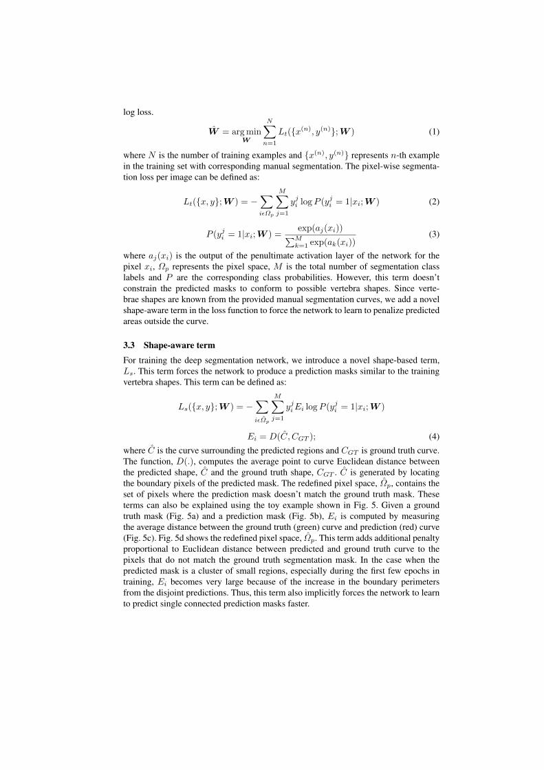
where C is the curve surrounding the predicted regions and CGT is ground truth curve.The function, D(.), computes the average point to curve Euclidean distance betweenthe predicted shape, C and the ground truth shape, CGT . C is generated by locatingthe boundary pixels of the predicted mask. The redefined pixel space, Ωp, contains theset of pixels where the prediction mask doesn’t match the ground truth mask. Theseterms can also be explained using the toy example shown in Fig. 5. Given a groundtruth mask (Fig. 5a) and a prediction mask (Fig. 5b), Ei is computed by measuringthe average distance between the ground truth (green) curve and prediction (red) curve(Fig. 5c). Fig. 5d shows the redefined pixel space, Ωp. This term adds additional penaltyproportional to Euclidean distance between predicted and ground truth curve to thepixels that do not match the ground truth segmentation mask. In the case when thepredicted mask is a cluster of small regions, especially during the first few epochs intraining, Ei becomes very large because of the increase in the boundary perimetersfrom the disjoint predictions. Thus, this term also implicitly forces the network to learnto predict single connected prediction masks faster.
(a) (b) (c) (d)
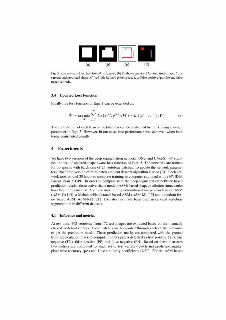
Fig. 5: Shape-aware loss: (a) Ground truth mask (b) Predicted mask (c) Ground truth shape, CGT
(green) and predicted shape, C (red) (d) Refined pixel space, Ωp: False positive (purple) and falsenegative (red).
3.4 Updated Loss Function
Finally, the loss function of Eqn. 1 can be extended as:
W = argminW
N∑n=1
Lt(x(n), y(n);W ) + Ls(x(n), y(n);W ) (5)
The contribution of each term in the total loss can be controlled by introducing a weightparameter in Eqn. 5. However, in our case, best performance was achieved when bothterms contributed equally.
4 Experiments
We have two versions of the deep segmentation network: UNet and UNet-S. ‘-S’ signi-fies the use of updated shape-aware loss function of Eqn. 5. The networks are trainedfor 30 epochs with batch size of 25 vertebrae patches. To update the network parame-ters, RMSprop version of mini-batch gradient descent algorithm is used [24]. Each net-work took around 30 hours to complete training in computer equipped with a NVIDIAPascal Titan X GPU. In order to compare with the deep segmentation network basedprediction results, three active shape model (ASM)-based shape prediction frameworkshave been implemented. A simple maximum gradient-based image search based ASM(ASM-G) [14], a Mahalanobis distance based ASM (ASM-M) [15] and a random for-est based ASM (ASM-RF) [21]. The later two have been used in cervical vertebraesegmentation in different datasets.
4.1 Inference and metrics
At test time, 792 vertebrae from 172 test images are extracted based on the manuallyclicked vertebral centers. These patches are forwarded through each of the networksto get the prediction masks. These prediction masks are compared with the groundtruth segmentation mask to compute number pixels detected as true positive (TP), truenegative (TN), false positive (FP) and false negative (FN). Based on these measurestwo metrics are computed for each set of test vertebra patch and prediction masks:pixel-wise accuracy (pA) and Dice similarity coefficients (DSC). For the ASM based
shape predictors, the predicted shape is converted to a prediction map to measure thesemetrics.
DSC =2TP
2TP + FP + FN(6)
pA =TP + TN
TP + TN + FP + FN× 100% (7)
These metrics are well suited to capture the number of correctly segmented pixels,but they fail to capture the differences in shape. In order to compare the shape of thepredicted mask appropriately with the ground truth vertebrae boundary, the predictedmasks of the deep segmentation networks are converted into shapes by locating theboundary pixels. These shapes are then compared manually annotated vertebral bound-ary curves by measuring average point to curve Euclidean distance between them, simi-lar to Eqn. 4. A final metric, called fit failure [20], is also computed which measures thepercentage of vertebrae having an average point to ground truth curve error of greaterthan 2 pixels.
5 Results
Table 1 reports the average median, mean and standard deviation (std) metrics overthe test dataset of 792 vertebrae for all the methods. The deep segmentation networksclearly outperform the ASM-based methods. Even the worst version of our framework,UNet achieves a 2.9% improvement in terms of pixel-wise accuracy and an increase of0.055 for Dice similarity coefficient. Among the two version of deep networks, the useof novel loss function improves the performance by 0.31% in terms of pixel-wise accu-racy. In terms of Dice similarity coefficient, the improvement is in the range of 0.006.Although, subtle, the improvements are statistically significant according to a pairedt-test at a 5% significance level. Corresponding p-values between the two versions ofthe network are reported in Table 1. Bold fonts indicates the best performing metrics.Interestingly, among the ASM-based methods, the simplest version, ASM-G, performsbetter than the alternatives. Recent methods [15,21], have failed to perform robustly onour challenging dataset of test vertebrae.
Table 1: Average quantitative metrics for mask prediction.
Pixel-wise accuracy (%) Dice similarity coefficientMedian Mean Std p-value Median Mean Std p-value
ASM-RF 95.09 90.77 8.98 0.881 0.774 0.220ASM-M 95.09 93.48 4.92 0.900 0.877 0.073ASM-G 95.34 93.75 4.48 0.906 0.883 0.066
UNet 97.71 96.69 3.047.17× 10−13
0.952 0.938 0.0487.76× 10−13
UNet-S 97.92 97.01 2.79 0.957 0.944 0.044
The average point to curve error for the methods are reported in Table 2. The deepsegmentation framework, UNet, produced a 35% improvement over the ASM-basedmethods in terms of the mean values. The introduction of the novel loss term in the
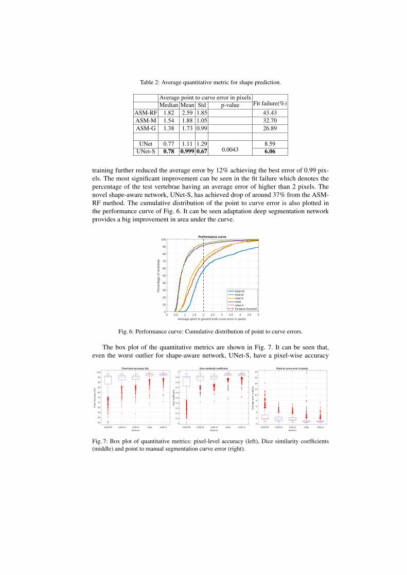
Table 2: Average quantitative metric for shape prediction.
Average point to curve error in pixelsFit failure(%)Median Mean Std p-value
ASM-RF 1.82 2.59 1.85 43.43ASM-M 1.54 1.88 1.05 32.70ASM-G 1.38 1.73 0.99 26.89
UNet 0.77 1.11 1.290.0043
8.59UNet-S 0.78 0.999 0.67 6.06
training further reduced the average error by 12% achieving the best error of 0.99 pix-els. The most significant improvement can be seen in the fit failure which denotes thepercentage of the test vertebrae having an average error of higher than 2 pixels. Thenovel shape-aware network, UNet-S, has achieved drop of around 37% from the ASM-RF method. The cumulative distribution of the point to curve error is also plotted inthe performance curve of Fig. 6. It can be seen adaptation deep segmentation networkprovides a big improvement in area under the curve.
0 0.5 1 1.5 2 2.5 3 3.5 4 4.5 5
Average point to ground truth curve error in pixels
0
10
20
30
40
50
60
70
80
90
100
Per
cent
age
of v
erte
brae
Performance curve
ASM-RFASM-MASM-GUNetUNet-SFit failure threshold
Fig. 6: Performance curve: Cumulative distribution of point to curve errors.
The box plot of the quantitative metrics are shown in Fig. 7. It can be seen that,even the worst outlier for shape-aware network, UNet-S, have a pixel-wise accuracy
ASM-RF ASM-M ASM-G UNet UNet-S
Method
50
55
60
65
70
75
80
85
90
95
100
Pix
el A
ccur
acy
(%)
Pixel-level accuracy (%)
ASM-RF ASM-M ASM-G UNet UNet-S
Method
0
0.1
0.2
0.3
0.4
0.5
0.6
0.7
0.8
0.9
1
Dic
e co
effic
ient
Dice similarity coefficient
ASM-RF ASM-M ASM-G UNet UNet-S
Method
0
2
4
6
8
10
12
14
16
18
Ave
rage
err
or in
pix
els
Point to curve error in pixels
Fig. 7: Box plot of quantitative metrics: pixel-level accuracy (left), Dice similarity coefficients(middle) and point to manual segmentation curve error (right).
(b)
(a)
(c)
(d)
(e)
(f)
(g)
(h)
(i)
(j)
Original Ground truth
ASM-RF ASM-M ASM-G UNet UNet-S
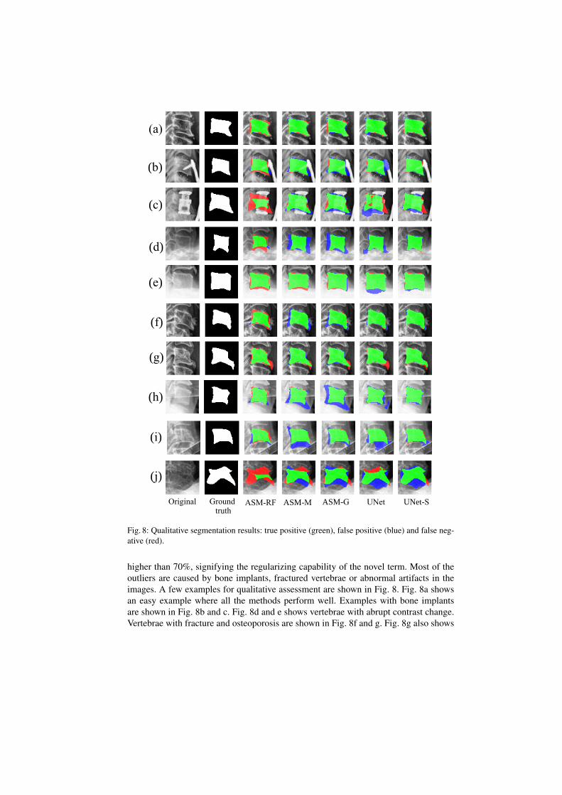
Fig. 8: Qualitative segmentation results: true positive (green), false positive (blue) and false neg-ative (red).
higher than 70%, signifying the regularizing capability of the novel term. Most of theoutliers are caused by bone implants, fractured vertebrae or abnormal artifacts in theimages. A few examples for qualitative assessment are shown in Fig. 8. Fig. 8a showsan easy example where all the methods perform well. Examples with bone implantsare shown in Fig. 8b and c. Fig. 8d and e shows vertebrae with abrupt contrast change.Vertebrae with fracture and osteoporosis are shown in Fig. 8f and g. Fig. 8g also shows
how UNet-S has been able capture the vertebrae fractures pattern. Fig. 8h and i showvertebrae with image artefacts. A complete failure case is shown in Fig. 8j. In all casesthe shape-aware network, UNet-S, has produced better segmentation results than itscounterpart.
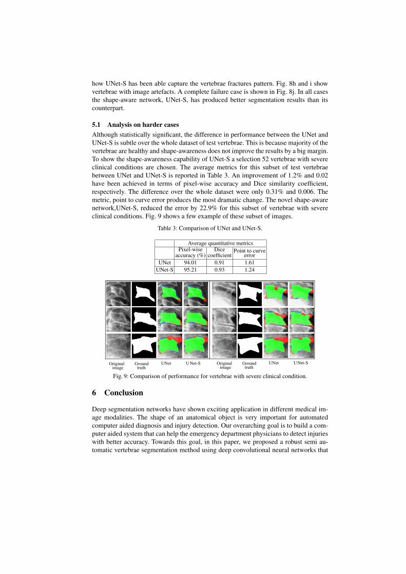
5.1 Analysis on harder casesAlthough statistically significant, the difference in performance between the UNet andUNet-S is subtle over the whole dataset of test vertebrae. This is because majority of thevertebrae are healthy and shape-awareness does not improve the results by a big margin.To show the shape-awareness capability of UNet-S a selection 52 vertebrae with severeclinical conditions are chosen. The average metrics for this subset of test vertebraebetween UNet and UNet-S is reported in Table 3. An improvement of 1.2% and 0.02have been achieved in terms of pixel-wise accuracy and Dice similarity coefficient,respectively. The difference over the whole dataset were only 0.31% and 0.006. Themetric, point to curve error produces the most dramatic change. The novel shape-awarenetwork,UNet-S, reduced the error by 22.9% for this subset of vertebrae with severeclinical conditions. Fig. 9 shows a few example of these subset of images.
Table 3: Comparison of UNet and UNet-S.
Average quantitative metricsPixel-wise
accuracy (%)Dice
coefficientPoint to curve
errorUNet 94.01 0.91 1.61
UNet-S 95.21 0.93 1.24
Original Ground truth
ASM-RF ASM-M ASM-G UNet UNet-S
Original Ground UNet UNet-S image truth
Original Ground UNet UNet-S image truth
Fig. 9: Comparison of performance for vertebrae with severe clinical condition.
6 Conclusion
Deep segmentation networks have shown exciting application in different medical im-age modalities. The shape of an anatomical object is very important for automatedcomputer aided diagnosis and injury detection. Our overarching goal is to build a com-puter aided system that can help the emergency department physicians to detect injurieswith better accuracy. Towards this goal, in this paper, we proposed a robust semi au-tomatic vertebrae segmentation method using deep convolutional neural networks that
incorporate the shape information in to achieve better segmentation accuracy. The pro-posed deep segmentation method has outperformed the traditional active shape modelbased approaches by a significant margin. In order to incorporate shape informationwith the mask prediction capability of the deep neural networks, a novel shape-awareloss function has been formulated. Inclusion of this novel term in the training providedsignificant quantitative and qualitative improvements. A maximum average pixel-levelsegmentation accuracy of 97.01%, Dice coefficient of 0.9438 and point to ground truthcurve error of less than 1 pixel has been achieved over a diverse dataset of 792 testvertebrae collected from real life medical emergency rooms. Currently, we are workingon a fully automatic localization framework to locate the vertebrae centers in arbitraryX-ray images. In the future, we will be using the segmented vertebrae column to auto-matically determine various clinical conditions like misalignment of the vertebral body,osteoporosis, bone density abnormality and type and severity of different vertebral frac-tures.
AcknowledgementsWe gratefully acknowledge the support of NVIDIA Corporation with the donation ofthe Titan X Pascal GPU used for this research.
References
1. A. Krizhevsky, I. Sutskever, and G. E. Hinton, “Imagenet classification with deep con-volutional neural networks,” in Advances in Neural Information Processing Systems 25(F. Pereira, C. J. C. Burges, L. Bottou, and K. Q. Weinberger, eds.), pp. 1097–1105, Cur-ran Associates, Inc., 2012.
2. K. Simonyan and A. Zisserman, “Very deep convolutional networks for large-scale imagerecognition,” arXiv preprint arXiv:1409.1556, 2014.
3. C. Szegedy, W. Liu, Y. Jia, P. Sermanet, S. Reed, D. Anguelov, D. Erhan, V. Vanhoucke, andA. Rabinovich, “Going deeper with convolutions,” in Proceedings of the IEEE Conferenceon Computer Vision and Pattern Recognition, pp. 1–9, 2015.
4. K. He, X. Zhang, S. Ren, and J. Sun, “Deep residual learning for image recognition,” inProceedings of the IEEE Conference on Computer Vision and Pattern Recognition, pp. 770–778, 2016.
5. E. Shelhamer, J. Long, and T. Darrell, “Fully convolutional networks for semantic segmen-tation,” IEEE Transactions on Pattern Analysis and Machine Intelligence, 2016.
6. S. Zheng, S. Jayasumana, B. Romera-Paredes, V. Vineet, Z. Su, D. Du, C. Huang, and P. H.Torr, “Conditional random fields as recurrent neural networks,” in Proceedings of the IEEEInternational Conference on Computer Vision, pp. 1529–1537, 2015.
7. H. Noh, S. Hong, and B. Han, “Learning deconvolution network for semantic segmentation,”in Proceedings of the IEEE International Conference on Computer Vision, pp. 1520–1528,2015.
8. O. Ronneberger, P. Fischer, and T. Brox, “U-net: Convolutional networks for biomedi-cal image segmentation,” in International Conference on Medical Image Computing andComputer-Assisted Intervention, pp. 234–241, Springer, 2015.
9. A. BenTaieb and G. Hamarneh, “Topology aware fully convolutional networks for histol-ogy gland segmentation,” in International Conference on Medical Image Computing andComputer-Assisted Intervention, pp. 460–468, Springer, 2016.
10. P. A. Yushkevich, J. Piven, H. C. Hazlett, R. G. Smith, S. Ho, J. C. Gee, and G. Gerig, “User-guided 3d active contour segmentation of anatomical structures: significantly improved effi-ciency and reliability,” Neuroimage, vol. 31, no. 3, pp. 1116–1128, 2006.
11. C. Pluempitiwiriyawej, J. M. Moura, Y.-J. L. Wu, and C. Ho, “Stacs: New active contourscheme for cardiac mr image segmentation,” IEEE Transactions on Medical Imaging, vol. 24,no. 5, pp. 593–603, 2005.
12. J. Weese, I. Wachter-Stehle, L. Zagorchev, and J. Peters, “Shape-constrained deformablemodels and applications in medical imaging,” in Shape Analysis in Medical Image Analysis,pp. 151–184, Springer, 2014.
13. A. A. Farag, A. Shalaby, H. A. El Munim, and A. Farag, “Variational shape representationfor modeling, elastic registration and segmentation,” in Shape Analysis in Medical ImageAnalysis, pp. 95–121, Springer, 2014.
14. T. F. Cootes, C. J. Taylor, D. H. Cooper, and J. Graham, “Active shape models-their trainingand application,” Computer Vision and Image Understanding, vol. 61, no. 1, pp. 38–59, 1995.
15. M. Benjelloun, S. Mahmoudi, and F. Lecron, “A framework of vertebra segmentation usingthe active shape model-based approach,” Journal of Biomedical Imaging, vol. 2011, p. 9,2011.
16. M. A. Larhmam, S. Mahmoudi, and M. Benjelloun, “Semi-automatic detection of cervicalvertebrae in X-ray images using generalized hough transform,” in Image Processing Theory,Tools and Applications (IPTA), 2012 3rd International Conference on, pp. 396–401, IEEE,2012.
17. M. Roberts, T. F. Cootes, and J. E. Adams, “Vertebral morphometry: semiautomatic de-termination of detailed shape from dual-energy X-ray absorptiometry images using activeappearance models,” Investigative Radiology, vol. 41, no. 12, pp. 849–859, 2006.
18. M. Roberts, E. Pacheco, R. Mohankumar, T. Cootes, and J. Adams, “Detection of vertebralfractures in DXA VFA images using statistical models of appearance and a semi-automaticsegmentation,” Osteoporosis International, vol. 21, no. 12, pp. 2037–2046, 2010.
19. M. G. Roberts, T. F. Cootes, and J. E. Adams, “Automatic location of vertebrae on DXA im-ages using random forest regression,” in Medical Image Computing and Computer-AssistedIntervention–MICCAI 2012, pp. 361–368, Springer, 2012.
20. P. Bromiley, J. Adams, and T. Cootes, “Localisation of vertebrae on DXA images using con-strained local models with random forest regression voting,” in Recent Advances in Compu-tational Methods and Clinical Applications for Spine Imaging, pp. 159–171, Springer, 2015.
21. S. M. M. R. Al-Arif, M. Gundry, K. Knapp, and G. Slabaugh, “Improving an active shapemodel with random classification forest for segmentation of cervical vertebrae,” in Compu-tational Methods and Clinical Applications for Spine Imaging: 4th International Workshopand Challenge, CSI 2016, Held in Conjunction with MICCAI 2016, Athens, Greece, October17, 2016, Revised Selected Papers, vol. 10182, p. 3, Springer, 2017.
22. T. F. Cootes, “Fully automatic localisation of vertebrae in ct images using random forestregression voting,” in Computational Methods and Clinical Applications for Spine Imag-ing: 4th International Workshop and Challenge, CSI 2016, Held in Conjunction with MIC-CAI 2016, Athens, Greece, October 17, 2016, Revised Selected Papers, vol. 10182, p. 51,Springer, 2017.
23. S. A. Mahmoudi, F. Lecron, P. Manneback, M. Benjelloun, and S. Mahmoudi, “GPU-basedsegmentation of cervical vertebra in X-ray images,” in Cluster Computing Workshops andPosters (CLUSTER WORKSHOPS), 2010 IEEE International Conference on, pp. 1–8, IEEE,2010.
24. S. Ruder, “An overview of gradient descent optimization algorithms,” arXiv preprintarXiv:1609.04747, 2016.