
Shape Analysis and Retrieval D2 Shape Distributions Notes courtesy of Funk et al., SIGGRAPH 2004.
59
Shape Analysis and Retrieval D2 Shape Distributions Notes courtesy of Funk et al., SIGGRAPH 200
-
Upload
alexis-bellamy -
Category
Documents
-
view
219 -
download
3
Transcript of Shape Analysis and Retrieval D2 Shape Distributions Notes courtesy of Funk et al., SIGGRAPH 2004.
Shape Analysis and Retrieval
D2 Shape Distributions
Notes courtesy of Funk et al., SIGGRAPH 2004

Outline:• Defining the Descriptor
• Computing the Descriptor
• Comparing the Descriptor (EMD)

D2 Shape DistributionsKey idea 1:
Map 3D surfaces to common parameterization by randomly sampling points on the shape.
Triangulated Model Point Set
By only considering point samples, the method avoids all problems of genus, connectivity, tessalation, etc.

D2 Shape DistributionsKey idea 2:
The distance between two points does not change if the points are translated or rotated:
||p1-p2||=||T(p1)-T(p2)||
for all T that are combinations of translations and rotations.
p2
p1||p1 -p
2 |||| T(p
1) - T(p2) ||
T(p1)T(p2)

D2 Shape DistributionsDefinition: For a set of points P, and a distance d, the value of the D2 Distribution at d is the number of point pairs whose pair-wise distance is d:
2
s.t. ,)(2D
P
dqpPqpdP
D2Model distance
prob
abili
ty

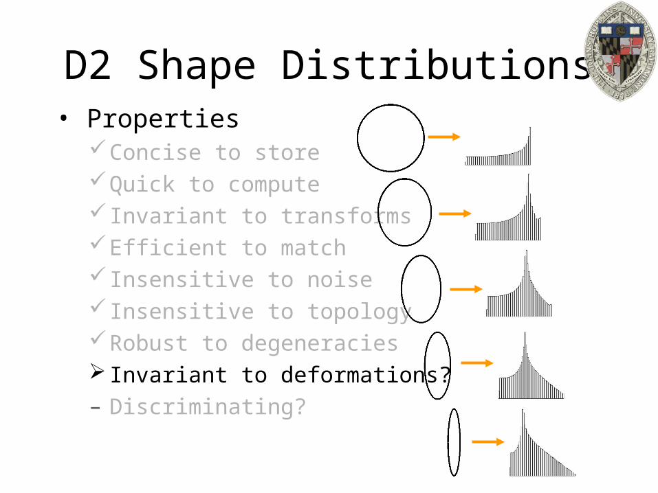
D2 Shape Distributions• Properties
– Concise to store?
– Quick to compute?
– Invariant to transforms?
– Efficient to match?
– Insensitive to noise?
– Insensitive to topology?
– Robust to degeneracies?
– Invariant to deformations?
– Discriminating?

D2 Shape Distributions• Properties
Concise to store?Quick to compute?
– Invariant to transforms?
– Efficient to match?
– Insensitive to noise?
– Insensitive to topology?
– Robust to degeneracies?
– Invariant to deformations?
– Discriminating?
512 bytes (64 values)
0.5 seconds (106 samples)
Distance
Probability
Skateboard

D2 Shape Distributions• Properties
Concise to storeQuick to compute Invariant to transforms?
– Efficient to match?
– Insensitive to noise?
– Insensitive to topology?
– Robust to degeneracies?
– Invariant to deformations?
– Discriminating?
TranslationRotationMirror
Normalized Means
Scale (w/ normalization)
Skateboard Porsche

D2 Shape Distributions• Properties
Concise to storeQuick to compute Invariant to transformsEfficient to match?
– Insensitive to noise?
– Insensitive to topology?
– Robust to degeneracies?
– Invariant to deformations?
– Discriminating?
Distance
Probability
Skateboard
Porsche

D2 Shape Distributions• Properties
Concise to storeQuick to compute Invariant to transformsEfficient to match Insensitive to noise? Insensitive to topology?Robust to degeneracies?
– Invariant to deformations?
– Discriminating?
1% Noise
D2 Shape Distributions• Properties
Concise to storeQuick to compute Invariant to transformsEfficient to match Insensitive to noise Insensitive to topologyRobust to degeneracies Invariant to deformations?
– Discriminating?

D2 Shape Distributions• Properties
Concise to storeQuick to compute Invariant to transformsEfficient to match Insensitive to noise Insensitive to topologyRobust to degeneracies Invariant to deformationsDiscriminating?
Line Segment Circle
Cylinder Cube
Sphere Two Spheres

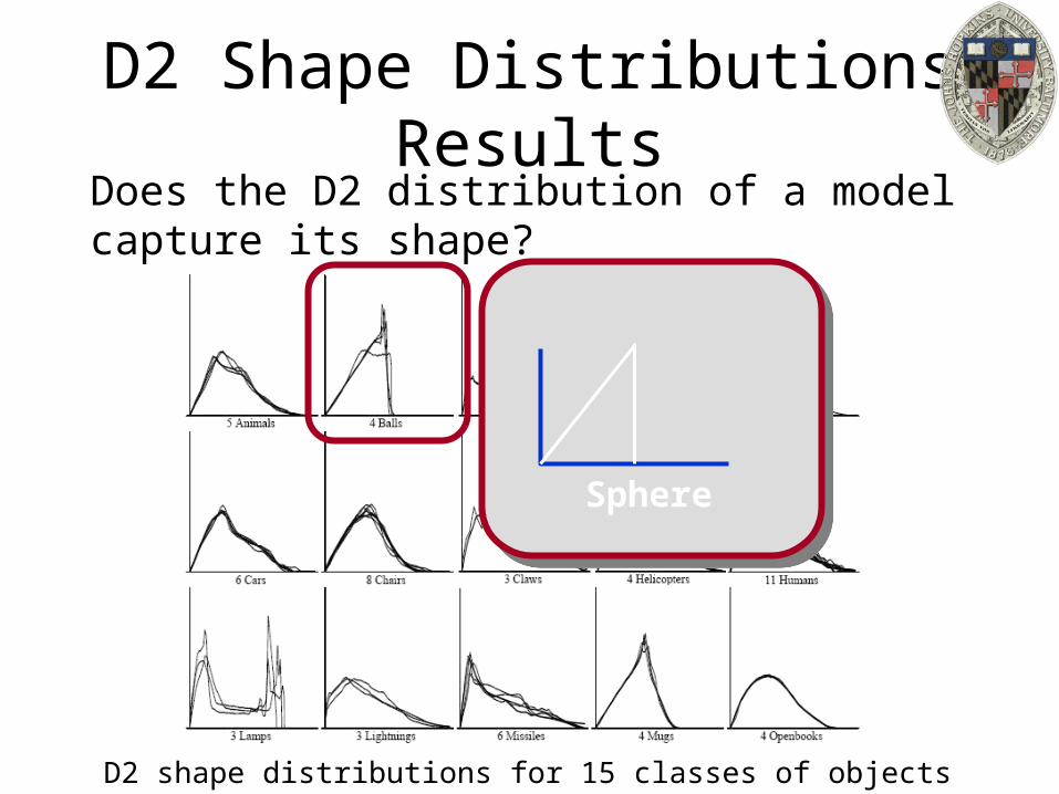
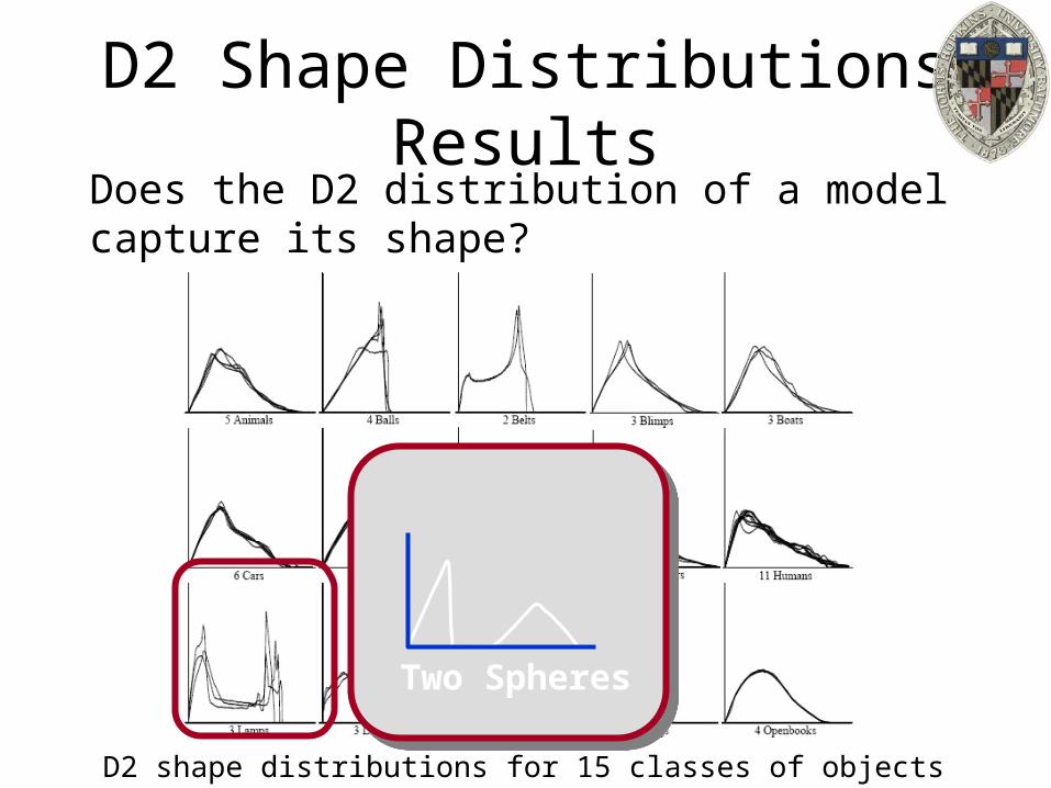
D2 Shape Distributions ResultsDoes the D2 distribution of a model capture its shape?
D2 shape distributions for 15 classes of objects

D2 Shape Distributions ResultsDoes the D2 distribution of a model capture its shape?
D2 shape distributions for 15 classes of objects
Line Segment

D2 Shape Distributions ResultsDoes the D2 distribution of a model capture its shape?
D2 shape distributions for 15 classes of objects
Circle

D2 Shape Distributions ResultsDoes the D2 distribution of a model capture its shape?
D2 shape distributions for 15 classes of objects
Cylinder
D2 Shape Distributions ResultsDoes the D2 distribution of a model capture its shape?
D2 shape distributions for 15 classes of objects
Sphere
D2 Shape Distributions ResultsDoes the D2 distribution of a model capture its shape?
D2 shape distributions for 15 classes of objects
Two Spheres
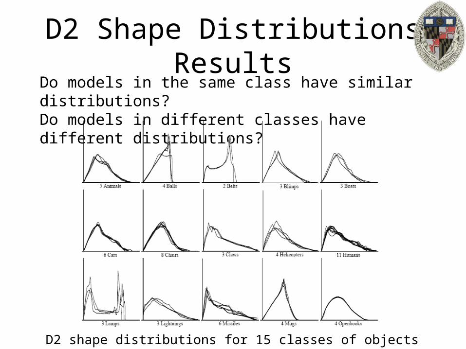
D2 Shape Distributions ResultsDo models in the same class have similar distributions?Do models in different classes have different distributions?
D2 shape distributions for 15 classes of objects

Princeton Shape Benchmark• 1814 classified models, 161 classes
• Evaluation metrics, software tools, etc.
http://shape.cs.princeton.edu/benchmark
51 potted plants 33 faces 15 desk chairs 22 dining chairs
100 humans 28 biplanes 14 flying birds 11 ships

Precision vs. RecallPrecision-recall curves
– Recall = retrieved_in_class / total_in_class– Precision = retrieved_in_class / total_retrieved
0 0.2 0.4 0.6 0.80
0.2
0.4
0.6
0.8
1
Recall
Pre
cisi
on
1
Ranked Matches
Query
44
77
11
55
22
88
66
33
99

Precision vs. RecallPrecision-recall curves
– Recall = 0 / 5– Precision = 0 / 0
0 0.2 0.4 0.6 0.80
0.2
0.4
0.6
0.8
1
Recall
Pre
cisi
on
1
Ranked Matches
Query
44
77
11
55
22
88
66
33
99
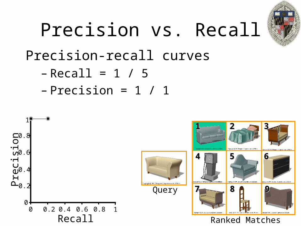
Precision vs. RecallPrecision-recall curves
– Recall = 1 / 5– Precision = 1 / 1
0 0.2 0.4 0.6 0.80
0.2
0.4
0.6
0.8
1
Recall
Pre
cisi
on
1
Ranked Matches
Query
44
77
11
55
22
88
66
33
99

Precision vs. RecallPrecision-recall curves
– Recall = 2 / 5– Precision = 2 / 3
0 0.2 0.4 0.6 0.80
0.2
0.4
0.6
0.8
1
Recall
Pre
cisi
on
1
Ranked Matches
Query
44
77
11
55
22
88
66
33
99

Precision vs. RecallPrecision-recall curves
– Recall = 3 / 5– Precision = 3 / 5
0 0.2 0.4 0.6 0.80
0.2
0.4
0.6
0.8
1
Recall
Pre
cisi
on
1
Ranked Matches
Query
44
77
11
55
22
88
66
33
99

Precision vs. RecallPrecision-recall curves
– Recall = 4 / 5– Precision = 4 / 7
0 0.2 0.4 0.6 0.80
0.2
0.4
0.6
0.8
1
Recall
Pre
cisi
on
1
Ranked Matches
Query
44
77
11
55
22
88
66
33
99

Precision vs. RecallPrecision-recall curves
– Recall = 5 / 5– Precision = 5 / 9
0 0.2 0.4 0.6 0.80
0.2
0.4
0.6
0.8
1
Recall
Pre
cisi
on
1
Ranked Matches
Query
44
77
11
55
22
88
66
33
99

D2 Shape DistributionsPrecision vs. recall on Princeton Benchmark
0%
50%
100%
0% 50% 100%Recall
Pre
cisi
on
D2Random

D2 Shape DistributionsPrecision vs. recall on Princeton Benchmark
0%
50%
100%
0% 50% 100%Recall
Pre
cisi
on
Gaussian EDTD2Random

Outline:• Defining the Descriptor
• Computing the Descriptor
• Comparing the Descriptor (EMD)

Computing From a Point SetGiven a point set P={p1,…,pn}, a resolution r, a max distance d, and an array d2:
GetD2(P,n,d,d2,r)c 0for i=1 to n
d2[i] 0for i=1 to n
for j=1 to i
t||pi-pj||if (t<d)
d2[(t/d)*r] d2[(t/d)*r] + 1c c + 1
for i=1 to nd2[i] d2[i]/c

Computing From a Point SetComputing the D2 distribution is easy if you have a point set. GetD2(P,n,d,d2,r)
c 0for i=1 to n
d2[i] 0for i=1 to n
for j=1 to i
t||pi-pj||if (t<d)
d2[(t/d)*r] d2[(t/d)*r] + 1c c + 1
for i=1 to nd2[i] d2[i]/c
Point Set D2 Distribution

Computing From a Point SetComputing the D2 distribution is easy if you have a point set.
How do you get a point set?(Most often, the query will bea collection of triangles.)
Triangulated Model
?
Point Set D2 Distribution
GetD2(P,n,d,d2,r)c 0for i=1 to n
d2[i] 0for i=1 to n
for j=1 to i
t||pi-pj||if (t<d)
d2[(t/d)*r] d2[(t/d)*r] + 1c c + 1
for i=1 to nd2[i] d2[i]/c

Getting a Uniformly Distributed Random Point Set
Goal:
Given a triangulated surface S={T1,…,Tk}, find n points uniformly distributed on model.
Definition: A distribution is uniformly distributed if the probability of a point being in some sub-region is proportional to the area of the sub-region.
Triangle Model Point Set (n=100) Point Set (n=1000)

AreasIf T=(p1,p2,p3) is a triangle, the area of T is equal to:
If S={T1,…,Tk} is a triangulated model, the area of S is equal to the sums of the areas of the Ti.
2
1312 ppppT
p1
p2
p3
(p2-p1)x(p3-p1)
(p2-p1
)
(p 3-p 1
)

Getting a Random PointTo generate a random sample point:
1. Randomly choose triangle Tj
which the point should be on.
2. Randomly choose a point in Tj.

Getting a Random Point1. Randomly choose a triangle Tj on which the
point should be.
The probability of a point being on triangle Tj isproportional to the area of a triangle:
ST
TP jj )(
SS surface theof Area
TT triangle theof Area
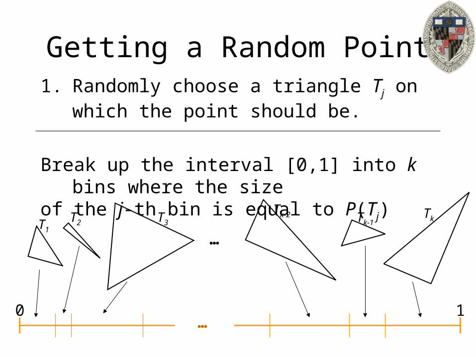
Getting a Random Point1. Randomly choose a triangle Tj on which the
point should be.
Break up the interval [0,1] into k bins where the sizeof the j-th bin is equal to P(Tj)
0 1…
…T1
T2 T3
Tk-2 Tk-1Tk

Getting a Random Point1. Randomly choose a triangle Tj on which the
point should be.
Generate a random number in the interval [0,1] andfind the index j of the bin it falls into.
0 1…
…T1
T2 T3
Tk-2 Tk-1Tk
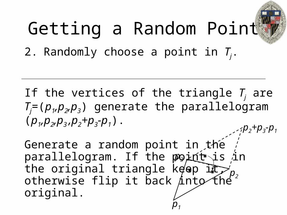
Getting a Random Point2. Randomly choose a point in Tj.
p1
p2
p3
p2+p3-p1
If the vertices of the triangle Tj are Tj=(p1,p2,p3) generate the parallelogram (p1,p2,p3 ,p2+p3-p1).
Generate a random point in theparallelogram. If the point is inthe original triangle keep it,otherwise flip it back into theoriginal.

Getting a Random Point2. Randomly choose a point in Tj.
p1
p2
p3
p2+p3-p1
To generate a random point in the parallelogram, generate two random numbers s and t in the interval [0,1]. Set p to be the point:
If s+t >1 the point will not bein the original triangle, flip itby sending:
)()( 13121 pptppspp
)1,1(),( tsts

Outline:• Defining the Descriptor
• Computing the Descriptor
• Comparing the Descriptor (EMD)

Earth Mover’s DistanceExample:
Supposing I am given the distribution of grades for a course over the past three years and I want to compare the distributions:
[Rubner et al. 1998]
0%
20%
40%
60%
80%
100%
0%
20%
40%
60%
80%
100%
Year 1 Year 2 Year 3
0%
20%
40%
60%
80%
100%
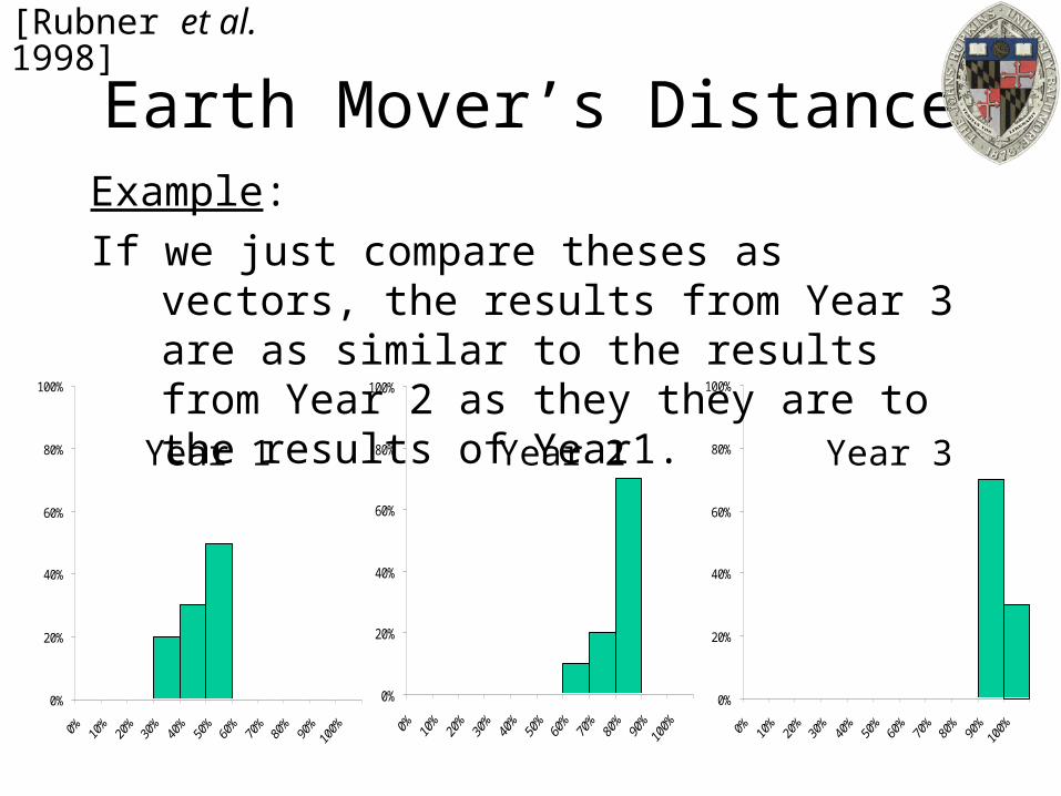
Earth Mover’s DistanceExample:
If we just compare theses as vectors, the results from Year 3 are as similar to the results from Year 2 as they they are to the results of Year1.
[Rubner et al. 1998]
0%
20%
40%
60%
80%
100%
0%
20%
40%
60%
80%
100%
0%
20%
40%
60%
80%
100%
Year 1 Year 2 Year 3

Earth Mover’s DistanceIdea:
Treat one distribution as hills, the other as valleys and find the minimum amount of work needed to be done to move earth from the hills to the valleys to flatten things out.
[Rubner et al. 1998]
0%
20%
40%
60%
80%
100%
0% 10% 20% 30% 40% 50% 60% 70% 80% 90% 100%
0%
20%
40%
60%
80%
100%
0% 10% 20% 30% 40% 50% 60% 70% 80% 90% 100%
-100%
-80%
-60%
-40%
-20%
0%
20%
40%
60%
80%
100%
0 % 1 0 % 2 0 % 3 0 % 4 0 % 5 0 % 6 0 % 7 0 % 8 0 % 9 0 % 1 0 0 %

Earth Mover’s DistanceApproach:Instead of comparing the values in each bin, compute
the amount of work needed to transform on distribution into the other.
Define the cost of moving d values from bin to i to bin j as:
Find the minimal amount of work that needs to be done to transform one distribution into the other.
[Rubner et al. 1998]
jidjid ),,(Work

Earth Mover’s DistanceChallenge:
Given distributions X={x1,…,xn} and Y={y1,…,yn}, set cij=|i-j| and find the values for fij that minimize:
subject to the constraints:
[Rubner et al. 1998]
n
i
n
jijijcf
1 1
n
ijij
n
jiij yfxf
11
and
cij= cost of moving from bin i to bin j
fij= amount of data moved from bin i to bin j
0ijf

Earth Mover’s DistanceSolution:
In general, this is the transportation problem and can be solved using linear programming.
For 1D histograms, this can be solved using the greedy algorithm.
[Rubner et al. 1998]
0%
20%
40%
60%
80%
100%
0% 10% 20% 30% 40% 50% 60% 70% 80% 90% 100%
0%
20%
40%
60%
80%
100%
0% 10% 20% 30% 40% 50% 60% 70% 80% 90% 100%
• Find the first non-empty bin.
• Move earth into first non-empty bin in the other histogram.
.1x3
Work=0

Earth Mover’s DistanceSolution:
In general, this is the transportation problem and can be solved using linear programming.
For 1D histograms, this can be solved using the greedy algorithm.
[Rubner et al. 1998]
0%
20%
40%
60%
80%
100%
0% 10% 20% 30% 40% 50% 60% 70% 80% 90% 100%
0%
20%
40%
60%
80%
100%
0% 10% 20% 30% 40% 50% 60% 70% 80% 90% 100%
• Find the first non-empty bin.
• Move earth into first non-empty bin in the other histogram.
Work=0.3
.1x4

Earth Mover’s DistanceSolution:
In general, this is the transportation problem and can be solved using linear programming.
For 1D histograms, this can be solved using the greedy algorithm.
[Rubner et al. 1998]
0%
20%
40%
60%
80%
100%
0% 10% 20% 30% 40% 50% 60% 70% 80% 90% 100%0%
20%
40%
60%
80%
100%
0% 10% 20% 30% 40% 50% 60% 70% 80% 90% 100%
• Find the first non-empty bin.
• Move earth into first non-empty bin in the other histogram.
Work=0.7
.1x3

Earth Mover’s DistanceSolution:
In general, this is the transportation problem and can be solved using linear programming.
For 1D histograms, this can be solved using the greedy algorithm.
[Rubner et al. 1998]
0%
20%
40%
60%
80%
100%
0% 10% 20% 30% 40% 50% 60% 70% 80% 90% 100%0%
20%
40%
60%
80%
100%
0% 10% 20% 30% 40% 50% 60% 70% 80% 90% 100%
• Find the first non-empty bin.
• Move earth into first non-empty bin in the other histogram.
Work=1.0

Earth Mover’s DistanceSolution:
In general, this is the transportation problem and can be solved using linear programming.
For 1D histograms, this can be solved using the greedy algorithm.
[Rubner et al. 1998]
0%
20%
40%
60%
80%
100%
0% 10% 20% 30% 40% 50% 60% 70% 80% 90% 100%
0%
20%
40%
60%
80%
100%
0% 10% 20% 30% 40% 50% 60% 70% 80% 90% 100%
• Find the first non-empty bin.
• Move earth into first non-empty bin in the other histogram.
Work=1.0
.2x4

Earth Mover’s DistanceSolution:
In general, this is the transportation problem and can be solved using linear programming.
For 1D histograms, this can be solved using the greedy algorithm.
[Rubner et al. 1998]
0%
20%
40%
60%
80%
100%
0% 10% 20% 30% 40% 50% 60% 70% 80% 90% 100%0%
20%
40%
60%
80%
100%
0% 10% 20% 30% 40% 50% 60% 70% 80% 90% 100%
• Find the first non-empty bin.
• Move earth into first non-empty bin in the other histogram.
Work=1.8
.5x3

Earth Mover’s DistanceSolution:
In general, this is the transportation problem and can be solved using linear programming.
For 1D histograms, this can be solved using the greedy algorithm.
[Rubner et al. 1998]
0%
20%
40%
60%
80%
100%
0% 10% 20% 30% 40% 50% 60% 70% 80% 90% 100%
0%
20%
40%
60%
80%
100%
0% 10% 20% 30% 40% 50% 60% 70% 80% 90% 100%
• Find the first non-empty bin.
• Move earth into first non-empty bin in the other histogram.
Work=3.3

Earth Mover’s DistanceAlternatively:
Compute the cumulative distributions:
Then the Earth Mover’s Distance between X and Y is:
So that for 1D histograms, the EMD can be expressed as a normed difference.
[Rubner et al. 1998]
i
jjxiCDX
1
)(
n
i
iCDYiCDXYXEMD1
)()(),(