Optimal Control of a Finite-Element Limited-AreaShallow-Water Equations Model

Xiao Chen

Department of Mathematics, Florida State University, Tallahassee, Florida

Email: xc06@fsu.edu

I. M. Navon

Department of Scientific Computing, Florida State University, Tallahassee, Florida

Email: inavon@fsu.edu

Dedicated to Professor Necnla; Andrei on the occasion of his 60th birthday.

Abstract: Optimal control of a finite element limited-area shallo\\' \vater equations model is explored with a viewto applying variational data assimilation(VDA) by obtaining the minimum of a functional estimating thediscrepancy bern'cen the model solutions and distrihuted observations. In our application, some simplifiedhypotheses are used, namely the error of the model is neglected, only the initial conditions are considered as thecontrol variables, lateral boundary conditions are periodic and finally the observations are assumed to be distributedin space and time. Derivation of the optimality system including the adjoint state, pennits computing the gradientof the cost functional with respect to the initial conditions which are used as control variables in the optimization.Different numerical aspects related to the construction (If the adjoint model and verification of its correctness areaddressed. The data assimilation set-up is tested fl.)r various mesh resolutions scenarios and different time stepsusing a modular computer code. Finally, impact oflarge-scale minimization solvers L-BFGS is assessed for variouslengths ofthc time windows.

Keywords: Variational data assimilation; Shallow-Water equations modeL Galerkin Finite-Element; Adjointmodel; Limited-area boundary condition.

Xiao Chen holds a M.Sc. degree in Applied Mathematics(2006) from Zhejiang University, lIangzhou, China.Currently, he is enrolled as a doctoral student in the department of mathematics al Florida State University, USA.His research interests include optimal control in Fluid Dynamics, four dimensional variational data assimilationmethod, probability and stochastic process, scientific computing and automatic differcntiation.

lonel Michael Navon graduated in Mathematics and Physics from Hebre""'lJniversity,Jerusalem and holds a M.Sc.in Atmospheric Sciences from the same University and a Ph.D. degree in Applied Mathematics from University ofWitwatersrand, Johmmesburg (J 979). lie is presently Program Director and Professor in the Department ofScientific Computing at Florida State University, Tallahassee, fL where he joined in 1985. He served previouslyas Chief Research Officer at National Research institute for Mathematical Sciences in Pretoria, South-Africa.(1975-1984) He is the author of more than 160 peer revic\ved high impact journal papers in areas of optimal control,data assimilation, parameter estimation, finite element modeling, large-scale numerical optimization and modelreduction applied to the geosciences that arc highly cited on 1&1 Wen of Science, along with more than 100scientific and technical reports .. He is also co-author or one book on adjoint sensitivity as \vell as contributor ofchapters in a dozen books including recently the Handbook for Numerical Analysis Series ( Elsevier) and a chapteron Data Assimilation in a recent Springer book on data assimilation.(2009). lie is a Pello\'.. of the AmericanMeteorological Society, was senior NRC fellow, fi:mncr Editor of major journals in applied mathematics andatmospheric sciences and is presently Editor of the International .Iournal for Numerical Methods in fluids (Wiley)and is included since 1992 in Who's Who in America. Prof. Navon educated 7 doctoral students in AppliedMathematics serving as their major Profcssor. His current research interests Il.lCUS on all aspects of POD modelreduction, data assimilation in the geosciences, large-scale optimization, optimal control and ensemble filters. Hisresearch is funded by the National Science Foundation and NASA He collaborates since 2002 with a majorresearch group at Imperial College as wel1 as vvith a research group 011 ocean data assimilation at lAP, AcademiaSinica, Beijing, China.

1. Introduction

This paper explores the feasibility of carryingout a modular structured variational dataassimilation (VDA) using a finite-elementmethod of the nonlinear shallow waterequations model on a limited area domain, inwhich we improve the methodology(Courtierand Talagrand 1987; Zhu et al. 1994) and

addresses issues in the development of theadjoint of a basic finite-element model.Specific numerical difficulties in the adjointderivation, for example, the treatment of theadjoint of the iterative process required forsolving the systems of linear algebraicequations resulting from the finite-elementdiscretizations using Crank-Nicholson time

Studies in Informatics and Control. Vol. 18, No. I, March 2009

-~--

41

(x,Y)E[O,L]x[O,D], f~O

2. Description of Problems

17= (u(x,y,t), v(x,y,t)) (3)

(5)

(4)

f = 2Qsin (J

is detined at a mean latitude (Jo' where Q is

the angular velocity of the earth's rotationand (J is latitude.

2.2 Initial and boundary conditions

The shallow-water equations requirespecifying appropriate initial and boundary

where u and v are the velocity components inthe x and Y axis respectively, ¢ = gh is the

geopotential height, h is the depth of thefluid and g is the acceleration of gravity. The

vector k is the vertical unit vector pointingaway from the center of the planet. Thescalar function f is the Coriolis parameterdefined by the (i-plane approximation:

f=J +b(y- ~)The Coriolis parameter

The shallow-water equations can be written as:

~-

cv + V . \7v+ \7 ¢ + / k x v= 0 (I)at

a¢ +\7'(¢v)=o (2)at

where Land D are the dimensions of arectangular domain of integration, v IS avector function:

2.1 Shallow-Water equations model onan/plane

The shallow-water equations model is one ofthe simplest forms of the equations of motionfor incompressible fluid for which the depth isrelatively small compared to the horizontaldimensions, which can be applied to describethe horizontal structure of an atmosphere. Theydescribe the evolution of an incompressiblefluid in response to gravitational and rotationalaccelerations (See Tan 1992 and Vreugdenhil1994 Galewsky 2004).

control set-up code organization is providedand illustrated in Appendix A.

differencing scheme (see Wang et al. 1972;Douglas and Dupont 1970) are explicitlyaddressed. The systems of algebraic linearequations resulting from the finite-elementdiscretizations of the shallow-water equationsmodel were solved by a Gauss-Seideliterative method. To save computer memory,a compact storage scheme for the banded andsparse global matrices was used (seeHinsman, 1975). We emphasize thedevelopment of the tangent linear (TLM) andthe adjoint models of the finite-elementshallow-water equations model and illustrateits use on various retrieval cases when the initialconditions are served as control variables.

The plan of this paper is as follows. The finite­element Galerkin method for the shallow­water equations model on an f plane, thederivation of its tangent linear model and itsadjoint are briefly described in section 2. Thefull finite element discretizations of the modelof the nonlinear shallow-water equationsmodel is described in section 3. Section 4introduces the optimal control methodologyincluding the development of the tangentlinear model and its adjoint as well asfonnulation of the cost functional aimed atallowing the derivation of optimal initialconditions reconciling model forecast andobservations in a window of data assimilationby minimizing the cost functional measuringlack of fit between model forecast andobservations. Particular attention is paid to thedevelopment of adjoint of iterative Gauss­Seidel solver. Verification of the correctnessof the adjoint is carried out in a detailedmanner for all stages of the calculations (i.e.TLM, adjoint and gradient test).

Set-up of numerical experiments and theexperimental design are detailed in Section 5.Basic assimilation experiments using a randomperturbation of the initial conditions asobservations and their results are presented.Particular attention is paid to the effectivenessof limited memory Quasi-Newton method L­BFGS for minimizing the cost functional inretrieving optimal initial conditions.

Various scenarios involving mesh resolution,different time steps as well as various lengths ofthe assimilation windows are tested andnumerical conclusions are drawn. FinallySection 6 presents Summary and Conclusions.A detailed description of the entire optimal

42 Studies in Informatics and Control, Vol. 18, No.1, March 2009

conditions. An initial condition is imposed as:

w(x,y,O) =<p(x,y), (6)or! { 0,/ ev' er! er!) ,

--= -----u-.-v- +W:(¢-¢)et ex 3y ex ay ¢

while solid wall boundary condition m y­direction is:

where the prime denotes a perturbationaround the basic state variables.

The geopotential <p(x,y) will be specified

later in the numerical experiments.

where state variables are

w = w(x,y,t) = (v(x,y,t),f(x,y,t») with

periodic boundary conditions are assumed inthe x-direction:

(I I)w'(x,y,t) = p(w(x,y,t»)w'(x,y,O)

By integrating the first order continuousadjoint model reversely in time, the gradientof a given cost functional .J is obtained bythe adjoint model solutions as follows:

u(T) = veT) = ¢(T) = 0

with final conditions equal to zeros:

The operator fonn of the discretized (9)-( I0)can be written as (see Navon et al. 1992)

[

U' (0)]V.J(wo)~V.J(uo,l'o'¢o)~w'(o)~ 1"(0)

¢' (0)

where w' =(u',v',¢') is the first order

adjoint variable vector, W", w,., W¢ are

weighting factors which are chosen to be theinverse of estimates of the statistical root-mean-square observational errors ongeopotential and wind componentsrespectively. In our test problem, values ofW = 10'm ',' and W =W =10-2 m-'s'f ' II I'

are used.

(7)

(8)

(10)

w(O,L,t) = w(O,D,t),

e¢' + V. (¢'v)+ V(¢v') = 0et

v(x,O,t) = v(x,D,t) = O.

2.3 Linearization of the Shallow-Waterequations model

The linearization of the shallow-waterequations model (I) - (2) can be written as:

ev' + v'.Vv + V. Vv'+V ¢'+ jk x ii'= 0 (9)at

The fonn above can also be writtenexplicitly (Jacques Blum, Franyois-XavierLe Dimet, 1. Michael Navon 2008) ascontinuous tangent linear model (TLM):

GU' ,au ,au 8t/J' au' au' ,-+U-+I'-+-+U' -+1'-- fi'=Oat tJx ~v ax a, ~v·

av' ,av I av 8t1/ av' av' ,-+u-+v -+-+u-+v-+ [u = 0et ex 0y0y ex Oy'

e¢' + a(¢'u) + a(¢'v) + e(¢u') + e(¢v') = 0at ex ey ox ay

and its first order continuous adjoint model withweighting forcing tenns may be written as:

Gu' { Gu' ~vu) ,av , at/) "--= -u---.- +v - +tv --¢'-!- +W(u-u)at Ex <} ax' ax "

av' {'Gu , av' ~uv) erf ) ,-= u--fu-v--:;----tf-!:- +~Tv-,!)Ct oy oy ex ov

where the control variable w'(x,y,O) is

the random perturhation variable of theinitial state variable w(x, y, 0), while

P (11'( -';, y, t ») represents the tangent linear

operator, so that we can obtain the controlvariable w'(x, v, t) that contains the

values of wind fields and geopotential fieldat the final time step.

Generally speaking, there are twoapproaches which could he employed forcalculating the gradient of the cost functionalwith respect to the initial conditions ofshallow water equations. The first approachis called continuous adjoint, in which weneed to differentiate the nonlinear shallowwater equations model with respect to itsinitial conditions first and then discretize itsadjoint PDE to compute the approximategradient of the given cost functional.Another approach is called discreteapproach, in which we need to approximatethe nonlinear PDE by a discretized nonlinearsystem of equations first and then

Studies in Informatics and Control, Vol. 18, No. I, March 2009 43

test function. Taking into account theboundary conditions (see Navon 1979), thesecond term of equation (13) vanishes so thatwe obtain the final expression for thecontinuity equation:

differentiate the discretized nonlinear systemwith respect to the parameters. The discreteadjoint approach is easy to implement withthe help of automatic differentiation tools,such as AD1FOR and TAMe. In thefollowing sections, we demonstrate themethodology of discrete adjoint to carryonthe VDA.

(dt,vi) - (¢N, V Vi) = o. (IS)

3. Discretization of the Shallow­Water Equations Model

3.1 Formulation of Galerkin Finite­Element model

Following the Galerkin FEM, the momentumequation (I) becomes:

(~ ,v,) +(v.w,v,) +(VifJ,v,) +(ik xv,v,) =0.( 16)

Studies in lnformatics and Control, Vol. 18, No. I, March 2009

(20)

where v; (I) and ifJ; (t) are the time­

dependent nodal values of wind fields andgeopotentia1 fields respectively.

Upon substituting (17) into (15)-( 16), oneobtains:

Wc may also write (19) explicitly as:

According to the definition (14), we maywrite (18) explicitly as:

J :;

v=L vj(flV;(x,y),ifJ=L ifJ;CtlV;(x,y) (17);-=1 /-1

Over each element, we denote wind fieldsand geopotentia1 fields

44

where the notation:

(dt ,vi) + (V . (ifJv), Vi) = 0 (12)

=>(~,v,)+ JV'(ifJv,v)-(~,Vv,)=O, (13)

defines the inner product when a function ismultiplied by the trial function Vi' where .

represents the inner product between tworeal vectors. In Galerkin FEM method, wechoose the trial function to coincide with the

We employ linear piecewise polynomials ontriangular elements in the formulation ofGalerkin Finite-Element model (I) - (2) forthe sake of of simplicity. Over each givenelement, a variable ~ can be written as (seeZienkiewicz 2005)

The advection terms in the continuityequation (2) are usually integrated by partsusing Green's theorem to shift the derivativefrom the variable to the basis function, whichyields:

where ~; (t) represents the scalar node value

of variable ~; at the node of the triangular

element, and Vj

represents a basis

function(interpolation function) defined bythe coordinates of the nodes.

3

~d = L~j(t)V;(X,y)j~l

M

(J,vi)= L J J](x,y).vidxdy (14)e!cmel1l.1

[

ilU J__I Vill I

ilv .. , Vi__I Vill }

+

, 3 " 1 ,,_I (A 2)W =-W --W +0 ul

2 2

where the state variables

W = w(x,y,t) = (v(x,y,I),¢(x,y,I)}

(23)

\(- "', V) )+ J", k , V = 0ji"Vk '

V,(u"v,)

ilVju.-­

J ilx

ilVjv-­'ax

ilVU __I

lilyoV

v--}I ily

At each time step the shallow-waterequations system was coupled, i.e. thesolution of each equation after one iterationat a given time step was used to solve theother two equations for the same iteration forthe same time step.

Upon introducing a finite differencediscretization in time into the continuityequation (20), which is the first to be solvedat a given time step. one obtains

3.2 Time integration

A time-extrapolated Crank-Nicholson timedifferencing scheme was applied forintegrating in time the system of ordinarydifferential equations resulting from theapplication of the Galerkin FEM (see Navon1979, 1987). The shallow-water equationssystem was then coupled at every time stepso that the equations become quasi­linearized (see Wang et al. 1972; Douglasand Dupont 1970), since an average is takenat time level ;, 1 and time level n ofexpressions, while the nonlinear advectiveterms are linearized by estimating them at

time level n +.!. using the following second-2

order approximation in time:

11 ilV 11' ilVjK, = U;'ViVk-'dA+ v,v,vk-·dA,

d., ex de ry(28)

(25)

(27)

(29)

M(U"" -u,,)+ ~I K (u n• ' +u")

j 1 2 2 J }

+ M(K~+I +K~ )+~IP =02 .J ,J 2

efe

where

M = If VYldA

and

11 .av 11 .ilVK , = vjv,u, il; dA + vjv,Vk-'dA.de de 0J

(26)

K = 11 "n+J V ilVk dA21 'f'k i ~ ,

de OX

In this continuity equation, we need to use

Crank-Nicholson to extrapolate u' and v·at the current time step so that we can

proceed to solve ¢n+1 at the next time step

from (u', v· ,¢") .

By introducing the same finite differencescheme into the u-momentum equations (21),one obtains:

where

(21 )

(22)

\ilV ) \ ilV)=:;> __.I Vj,V

i+ UkVkVj __i,Vi

ill ilx

+\V'VkV j il~ 'V,)+\¢k c; ,V,)

+(JU,Vk,vi!=O.

and

Studies in Informatics and Control, Vol. 18. No.1, March 2009 45

In order to implement boundary conditions inthe Galerkin finite-element model, we haveadopted the approach suggested by Payne andIrons (see Payne 1963) and mentioned byHuebner (see HuebnerI975). This approachconsists in modifying the diagonal terms oftheglobal matrix associated with the nodalvariables by multiplying them by a large

number, say 10'6 (chosen with a view to thesignificant number of digits possible with thegiven computer and the size of the fieldvariables), while the corresponding term in theright-hand vector is replaced by the specifiedboundary nodal variable multiplied by thesame large factor times the correspondingdiagonal term. This procedure is repeated untilall prescribed boundary nodal variables havebeen treated (see Navon 1979). variables havebeen treated (see Navon 1979).

(30)

(31 )

P, = - If fv;V, V,dA.ell'

+M(Kn"+Kn)+MP =0,2 31 31 3

Finally, from the v-momentum equation(22), one obtains:

M(v.n+' _v n )+ tlt K (v'''' +v n)

I J 2 J J )

In this a-momentum equation, since we

already know the most recent solution ¢""from solving the continuity equation above,

we only need to extrapolate v' at the currenttime step so that we can proceed to solve

11+1U at the next time step from

(un, v' ,r').

and the discretized form of the numerical S­W equations model can be written as:

4. Optimal Control of GalerkinFinite-Element Model

4.1 Brief descriptions of Discrete TLMand Adjoint Techniques

The S-W equations model can be written as:

whereav

K = II ';+'vv _.I dA3 Uk i kete ax

av+ If v;vy, ~_.I dA

ere cy

K = II ,;;n+'v av, dA31 If'k I a '

de Y

P3 = If fat'V,V,dA.efe

(32)

(33)

(34)

aX(t) = F(X(t))at (35)

subject to the strong constraint, assummg

In its general form, the 4D-Var dataassimilation, is defined as the minimization

with respect to the initial condition X o of

the following discrete cost functional:

where initial condition X 0 is the control

variable for the given numerical S-W equations

model, Mo., is the predefined discretized

nonlinear S-W equations model forecast

operator, mapping the initial condition X o into

the model solution X, at time t,.

(36)In this v-momentum equation, since wealready know the most recent solution forboth .r n " and ani I at the current time step,we don't need any extrapolations at thecurrent time step and we can proceed

I nil h . ~to SO ve V at t e next tnne step ,rom(u n+1

, VII ,¢I1+I).

3.3 Gauss-Seidel iterative method forthe compact matrix of the Galerkinfinite-element model

In this Galerkin finite-element model, acompact matrix form was adopted due to thelocal support property over the trianglemesh. In particular, the N x N global matrix,assembled from each small element matrix,has at most seven nonzero elements at eachrow of the matrix. Hence, we can store theglobal matrix into a compact matrix of sizeN x 7. (see Zhu, Navon and Zou 1994).

46 Studies in Informatics and Control, Vol. 18, No.1, March 2009

VJ = VJ b + VJ" (40)

where the first term VJh can be easilyobtained as:

(42)

(.r(xo )} = JO(X o + X;,)-J"(X o)

= I H;(O~l(H,(X,)-y,)Y x~.1'=0

"J = J" +J" = J" + L (r), (39)

,.,,-()

where J hand J" are the background andobservation terms respectively.

In order to obtain the optimal initialconditions of shallow water equations modelthat minimizes J above, the gradient of Jneeds to be calculated with respect to thecontrol variable X o as:

and the second tenn VJ" requires theadjoint model integration which shall bebriefly derived as follows:

On the one hand, consider the change in thecost functional J resulting from a small

perturbation X~ in the initial condition ,

which can be written as:

that the model is perfect, so that thesequence of model states X, at time I,.

must be a solution for the given modelequations, where B is the background

covariance matrix, X, is the S-W equations

model solution at time I" 0, is the

observation error covariance matrix at time

I" H,. is the observation operator at time

I,. , representing projection of model

variables into the observational variables.

Since the M 0 ,,(Xo) IS a nonlinear

operator, the 4D-Var dala assimilationmethod becomes a nonlinear constrainedoptimization problem, with respected to thecontrol variable X o and it is very difficult to

solve. Fortunately, it can be greatlysimplified with two hypotheses.

The first hypothesis is the causality, in whichthe forecast model can be expressed as theproduct of intermediate forecast steps, sothat the nonlinear S-W equations model

forecast operator M o~, can be factorized

into MO----j.r=M,M,_I'··M1

, where each

operator M, denotes the discretized

nonlinear forecast operator step from time ;'1

to r and we have X, = M,.X'_l . Hence, by

recurrence, we have X, = M,. M,_I ...M I Xo.

where M, represents the linearization of the

discretized nonlinear S-W equations modelforecast operator.

Another hypothesis is that, at each time stepfrom both from r-I to r, we obtain that the

linearization of observation operator H,. can

be written as H" and that forecast operator

M,. can also be linearized so that the the

predefined discretized nonlinear S-Wequations model forecast operator can bedifferentiated(perturbed) to obtain a so­called tangent linear model(TLM) :

(44)

Furthermore, we are capable to find the gradientof the cost function by using the adjoint of theTangent Linear Model of the given nonlineartime-dependent discrete Galerkin FEM model(see Navon et al. 1992).

By comparing (41) (42) (43) together, we obtain

VJ(X,,) = B-J (X - Xb

)

+I M;H;O~'(H,(X,)- Y,r1'-0

On the other hand, to first order we can writethe Taylor expansion ofJ as:

(38)X'(t,) = M,X;,

4.2 Adjoint of Galerkin Finite-Elementmodel

Under those hypotheses, the quadratic costfunctional above can be written as asummation as:

Twhere M, represents the adjoint of model

at the r'" time step while the weighted

differences H;O~'(H,(X,)-V,) are

forcing terms which can either be added tothe adjoint variables whenever an

Studies in Informatics and Control. Vol. 18, No.1. March 2009 47

observational time is reached or can beinitialized at the initial time stage if they areavailable at that time.

The basic techniques in coding the adjointmodel above involves:

• Reset some temporary variables to zeroswhen using them in different statements;

• Saving and loading the state variablescalculated in the forward model;

• Identifying the reused adjoint controlvariables in all the subroutines;

Reset the accumulations of reusedadjoint variables to zeros when oneperiod of accumulation is finished;

- Finish the accumulations of reused adjointvariables only when calculating backwardsinto its first use;

• Handle the adjoint of iterative solversuch as Gauss-Seidel;

• Handle the adjoint of boundaryconditions;

• Identifying the inputs and outputs ofeach subroutine and the whole program;

• Make adjoint subroutines and parametersgeneric so that they can be reused fordifferent adjoint variables withoutrewriting them over and over again.

4.2.1. Adjoint of iterative solver

The challenging part in the development ofadjoint for nonlinear time-dependent discreteGalerkin Finite-Element model consists in thetreatment of the Gauss-Seidel iterativeprocedure to solve the continuity equationsystems and u-momentum equation systems aswell as v-momentum linear systems, becausesome of the control variables to be solved atthe current iteration level are reused whilesome are not (see Zhu, Navon and Zou 1994).

The key issues related to developing theadjoint of Gauss-Seidel iterative procedureare as follows:

We need to record the maximum number ofthe iterations when we integrate the nonlinearmodel forward in time, then, in order to obtainthe adjoint of the Gauss-Seidel iterativeprocedure, the relationship of being reusedamong all the control variables must beanalyzed. Finally, since the piecewise lineartriangular Galerkin Finite-Element model has a

local support of at most six nodes, while theminimum number of nodes is four when thenode is on the boundary. Hence, the variablevalue at any given node inner or boundary isrelated to no more than six neighboring nodessurrounding it, and sometimes they are inputvariables and sometimes they are outputvariables. We are only concemed with theinput variables when we speak about thereused variables, in other words, some of inputvariables in the iterative procedure are reusedwhile other input variables are not, dependingon the position in the grid as well as level oftht:: iteratiuns itself.

In addition, some control variables are firstlyused in the setup of the continuity system and itwill be used later twice in the setup of the u­momentum system. When dealing withsituation to reuse adjoint variables in theadjoint code, we need to save the accumulatedreused adjoint variables when calculatingbackwards into its first use. In other words,when we write the adjoint code, we needrestore all the following accumulations into itsfirst use when we finish the accumulation ofreused adjoint variables.

4.3 Verification of correctness of theTLM and adjoint

The space increments used in this section areLlx = "'y = 200km , while in the section 5, we

will adopt "'X = 4v = 400km for convenience.

4.3.1. TLM test

Prior to checking the correctness of the adjointmodel, we need to check the correctness of thediscrete TLM (Figure 1). One idea is toconsider a state vector X and a perturbation X'so that we can use Taylor expansion to verifythe correlation between nonlinear GalerkinFEM and its corresponding TLM:

w(a) = G(X + aX')- G(X) = I + O(a) (45)aP(X') ,

where G denotes the nonlinear Galerkin FEMand P represents its TLM operator, a definesthe perturbation factor. Both the nonlinearGalerkin FEM and its TLM are integrated for a5-hours period with various a valuesdecreasing, and the results show that thecorrelation between Nonlinear Galerkin FEMmodel and its TLM is almost equal to one asa tends to zero.

48 Studies in Informatics and Control, Vol. 18, No. I, March 2009

Therefore, if the TLM test can be correct, weonly need to code the adjoint model directly fromthe discrete TLM by rewriting the code of TLMstatement by statement in the opposite direction.This simplifies not only the complexity ofconstructing the adjoint model but also avoids theinconsistency generally arising from thederivation of the adjoint equations in analyticform followed by the discrete approximation(dueto non-commutativity of discretization andadjoint operators).

some issues where we need to be careful, whenrunning the test. First, we need to make sure allthe state variables have been saved when weintegrate TLM forward and restored or loadedwhen we integrate its adjoint backward. Second,we may need to run the different inputs to makesure we go through a rigorous check of theadjoint code into each single part of it. Finally,the results obtained illustrated that a 13 digitsaccuracy can be achieved in the input/output testsby using DOUBLE PRECISION.

TLM Test: Mesh 3U' 30, dt =IBOOs, WindOW = 5h

x

~1

-'

•. , • I.

"C-,-.Cc,e---' ----:c---C- ;~logl".)

4.3.3. Gradient test

We also tested the accuracy ofthe gradient ofthecost function by using the so-called a test asfollows (Figure 2):

F(a) = J(X+aX')-J(X) =l+O(a) (47)a(VJy(VJ)

and the results show that the vector we obtainedfrom the adjoint model is almost equal to thegradient as a decreasingly tends to zero, if a isnot too close to the machine accuracy(see Navon1992).

where X represents the perturbation of input ofthe Galerkin FEM model, while the TLMdenoted by P represents either a single DO loopor a subroutine. Each of them has its adjointimage DO loop or a subroutine, respectively. Theleft hand side involves only the tangent linearcode, while the right hand side involves also theadjoint code. When we implement it, we first runthe TLM code and use the output vector as theinput vector of the adjoint calculation. There are

Figure J. Correlation between NonlinearGalerkin FEM model and its TLM. where a

defines the perturbation factor

In addition, we also use an altemative idea to testthe TLM (and thus the adjoint). It's called thecomplex-step derivative approximation. It isreasonably straightforward to implement, and itrequires only slight modifications in the forwardmodel code. The feature of this method is that itcan avoid some cancellations in the finitedifference calculation that will result in the loss ofdigit accuracy (see Martins 2003).

4.3.2. Transpose test

The correctness of the adjoint model checked byfollowing the algebraic expression:

_4 _?

logr,,)

IOQ(ul

30 . 30, window = ?4h. dt ~ 1800s. pen 0.' %Oradlunt Test. Mesh

::L""-12 10 -8 -~

Figure 2. Gradient Test: (a) variation ofF(a)with respect to log a and (b) variation of

10g(F(a) -I) with respect to log a, where a

defines the perturbation factor

0'---'--------------12 1() -8

Gradient Test: Mc,h - JO . 30, w,ndow ~ 24h, dl 18005. pert ~ O. 1%------'--,

(46)(PXY (PX) = XT (p T (PX)),

Studies in Informatics and Control. Vol. 18. No. I, March 2009 49

5. Numerical Experiments

5.1 Description of problem

The test problem used here adopts the initialconditions (Figure 3) from the initial heightfield condition No.1 of Grammeltvedt (seeGrammeltvedt 1969):

h(x,y) = H o + HI tanh(9(DI2 - y»)2D (48)

+ H,( II COSh'( 9(D/~ - y»))Sin( 27:)

where this initial condition has energy in wavenumber one in the x-direction.

The initial velocity fields were derived fromthe initial height field using the geostrophicrelationship:

(49)

The dimensional constants used here are:

L ~ 4400km;D = 6000km; 1 = IO-'s I

,8 = 1.5 x 10 II S·l m I; (50)

!( = 10ms I; H 0 = 2000 m;

HI = 220m;H, = 133m.

and the space increments used here are

b.x = ~v = 400km (51)

Mesh = 15 • 15 contour from 22000 to 18000 by 500

0.9

08

0.7

0.6

~ ·-18006---------- ------'18000--- ------------------4 BOOa--

18500

0.51900019500

00000.4 'l: SOO

'2,.°,,0000.3 '2.

0.2

o 1 --22000-----

'/850019000

185'&JlSOO_2150027000

22000 - --22000

21500

0.2 0.4 06 0.8

50

(a) initial geopotential

" """'",,,,,,,,.,.,,,,.. ,,,,,,,,,,,,,,,"

(b) initial wind-field

Figure 3. Initial condition:(a) Geopotential tield for the Grammeltvedt initial condition. (b)Wind field calculated from the geopotential field by the geostrophic approximation.

Studies in Informatics and Control, Vol. 18, No.1, March 2009

------,----- /18000 .

1B;oo

'00001-;~,ffi!f)

2O\~j

21000

l'',900n

19500

?;r;oo§ l

ofJ"8

,~ ~

____._.1 , _•.=L.:'._ ..

0" CoJ 0., 0.f, 'd 00

(a) perturbation of initial geopotential

~.. O.'.~...".'0.... .

l

"_02L-__

o 02 0.4 0.8

(b) perturbation of initial wind-field

Figure 4. 5% random perturbation of geopotential and as well as the wind fields of theshallow-water equations model

Studies in Informatics and Control, Vol. 18, No.1, March 2009 51

5.2. Perturbation of initial conditions

We applied a 5% unifonn random perturbations(Figure 4) on the initial conditions in order toprovide twin-experiment "observations" and wealso computed the errors between the retrievedinitial conditions related to the perturbed dataand the reference state variables.

5.3 Retrieving the optimal initialconditions by applying

L-BFGS

The accuracy of a short-range numericalweather prediction greatly depends on theinitial and boundary conditions. The followingexperiments illustrate the technology to retrievethe optimal initial condition trom a noisy initialconditions. First, we randomly perturb theinitial conditions to generate the so-calledobservations at each time step. Second, wegenerate another rondom perturbations of theinitial conditions to obtain a initial guess of theinitial conditions in the optimization. In thispaper, we tried limited quasi-Newton method ofLiu and Nocedal (1980,1989) and Richard andNocedal (1995) to minimize the misfit betweenmodel solutions and artificial observations. Thecode is written in FORTRAN90 modularizedwith the control variables allocatable, so thatany different mesh size can be tested in thiscode with a high accuracy. We also tested thedifferent time steps as well as different dataassimilation windows. The control variables areall defined as DOUBLE PRECIS10N so that avery high accuracy of approximation of thegradient of the cost fimctional with respect tothe initial conditions can be achieved. In L­BFGS, we setup the number seven as thenumber of corrections (AJ=c7) (See Liu andNocedal 1989).

5.3.1. Testing different observations

The first experiment (Figure 5 and Figure 6) isperfonned on a short assimilation window for12 hours with a small mesh size consisting of15 x 15 grid points and we use a unconstrainedminimization algorithm L-BFGS to minimizethe cost fimctional. The adjoint model isintegrated backward in time, with a forcingterm being added, consisting of the differencebetween forecast and observation, interpolatedat the same time and space location every time

when an observation is encountered. We foundout (Table 1) ifwe use 5% perturbation for bothobservations and initial guess, the L-BFGSconverges in 31 iterations with 108 fimctionevaluations to converge to prescribed tolerance& ~ 1(Til (Figure 7), but if we use 1% randomperturbations, it will only take 28 iterations with99 fimction evaluations to converge, whichmeans both good observations and good initialguess will reduce the assimilation time required.

Table 1. L-BFGS: Data assimilation window ~

12h, L'.x ~ L'.y ~ 400km , M ~ 1800s, andminimization convergence tolerance.

Random Iterations Functionoerturbations evaluations

5% 31 1081% 28 99

Furthennore, if we extend the assimilationwindow trom 12 hours to 48 hours, the L­BFGS minimization fails to achieve theprescribed tolerance no matter how accurate theobservations and initial guess we choose for theoptimization algorithms. If the mesh size is toocoarse, say 5 x 5 grid points, even if we use 12hours assimilation window, we will still fail toconverge by using L-BFGS, which meanseither a too large assimilation window or a toosmall mesh size will affect the ability of the L­BFGS algorithm to converge to achieve theprescribed tolerance.

5.3.2. Testing different mesh resolutions

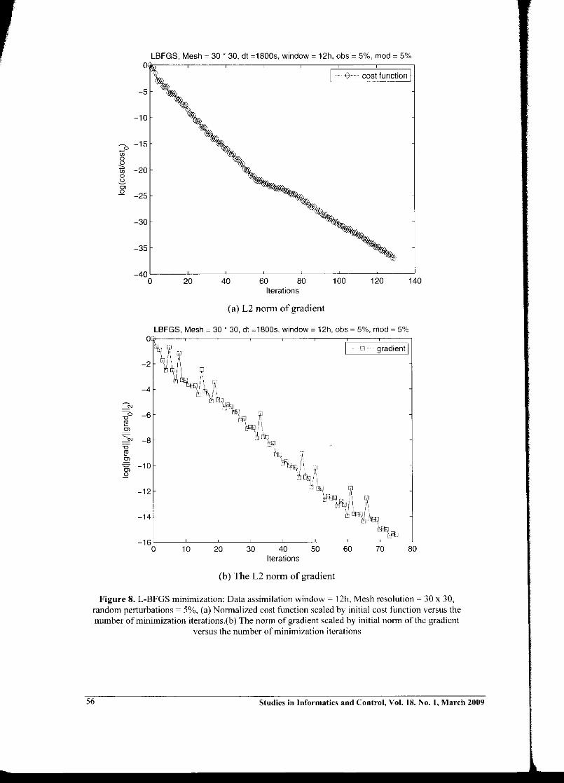
By increasing the mesh resolution from 15 x 15to 30 x 30 (Figure 8) and still using L-BFGS,we found out that we can achieve a strictertolerance 6- ~ 10 "', although it requires moreiterations and fimction evaluations to converge(Table 2). Hence, it can be observed that therate of the convergence of the cost fimctionalassociated with the coarse mesh is faster thanthe rate of convergence corresponding to thefme-resolution models, however, the value ofthe cost fimctional associated with the finemesh can be reduced to achieve a higher levelof tolerance that is by five orders of magoitudebetter than minimization of the cost fimctionalachieved for the coarse mesh.

52 Studies in Informatics and Control, Vol. 18, No.1, March 2009

Table 2. Results of using L-BFGS: dataassimilation window ~ 121t, Ax = I'>y = 200km ,

mesh resolution~ 30 x 30, 1'>1 ~ 1800s, andminimization convergence tolerance l: ::::0 10 16

Table 3. Results of using L-BFGS: data assimilation",indow ~ 12h, ,',x ~ ,',y = 400km , random

perturbations ~ 5%, 1'>1 ~ 900s, and tolerance ofconvergence ofminimization is &' = 10-15

•

Random Iterations Functionperturbations evaluations

5% 42 1621% 38 149

mesh size Iterations Functionevaluations

IS x 15 28 9730 x 30 35 140

200 8 \,~,

'8il.l 1

0.'

,(j) -}+, -200 §,,''0 ;;

/'f,

Figure 5. Data assimilation window ~ 12h. L'>x = I'>y =400km , random perturbation ~ 5%.The contours of difference between retrieved initial geopotential and true initial

geopotential are plotted.

5.3.3. Testing different time steps

By decreasing the time length from 1800s to900s while keeping an identical dataassimilation window of i2 hours, whichrequires more time steps, we can achieve aconvergence of minimization with tolerance

G = 10-15 by using a coarse mesh size~15xl5,

which is beneficial especially when there arenot enough observations ofa fine mesh in spaceavailable everywhere but we could have theability to measure them for every short timestep length, we may still retrieve a very highaccuracy of optilnal initial conditions byshrinking each time step length and expandingnumber ofdata assimilation steps (Table 3).

This can also be explained by noting that theresults from the fine mesh integrated contain morcsmall-scale features than the corresponding onesfrom the coarse mesh integrated, and thedimension of the control variables also impactsupon the convergence rate so that the retrievalwith tine-mesh model data becomes moredifficult. The presence of small-scale features inan increase in the condition number of the Hessianof the cost function of the fine-mesh resolutionmodel due to the introduction of smalleigenvalues in the spectrum of the Hessian(seeAxellson and Barker 1984). This situationbecomes more apparent when the dataassimilation is carried after a long time window ofassimilation allowing reflections from limitedboundaries thus causing short wave number noisycontaminations.

Studies in Informatics and Control, Vol. 18, No. I, March 2009 53

The contour of difference between retrieved initial u and true initial u

() 0

0.9 00

0.8 00 ()()

0.7 0 ()0 0

00.6

\ -0.2 0.2 0

o ~",.:;tO0.5 'V .~,: 0

0:;:l P, 0" 0.2 0 ,~ 1\ I o.:f?...'J 0

.... 0-0.4 0.4 C' ',.0 () 00.4 0

0 '0::.> '0 0 0·2." .",

0.3 0 0 /~." 'i1-

" 0 ~li'2 «. ""Cy0 -~'2

0.2 ()"-' ()"-'0

0.1 0

O~ 0 ()0

0 0.2 0.4 0.6 0.8

(a) The contour of difference between retrieved initial u-momentum and trueInitial u-momentum

The contour of difference between retrieved initial v and true initial v

0.9

()o

0.8

0.7

o0.6

'" '"

0.5

0.2~

o

o

-0.5

()

'"

0.5<:>

0.1

0.80.60.4oL-_-~---~---~ ~ .-J

o 0.2

(b) The contour of difference between retrieved initial v-momentum and true initialv-momentum

Figure 6. Data assimilation window ~ 12h. & ~ t-y ~ 400km • random perturbation ~ 5%. (a) The

contours of difference between retrieved initial u-momenturn and true initial u-momentum from ­0.5 to 0.5 by 0.2 are displayed. (b) The contours of difference between retrieved initial v­

momentum and true initial v-momentum from -0.3 to 0.3 by 0.05 are also displayed.

54 Studies in Informatics and Control, Vol. 18, No.1, March 2009

Mesh = 15 ~ 15, dt =1800s, window = 12h, obs = 5%, mod = 5%

----<} cost function I-5

-10

;;0-150

uCO>~

0u

-20c;.Q

-25

-30

-350 10 20 30 40

Iterations50 60 70

(a) Cost function

Mesh = 15' 15, dt =18008, window = 12h, obs = 5%, mod = 5%

I ---B--- gradient I

-12

-14

-16 L-_.~__~_ -~--.~----c~-._~--~.=-----='

o 10 20 30 40 50 60 70 80Iterations

(b) L2 norm of gradient

Figure 7. L-BFGS minimization: Data assimilation window ~ 12h, ill: = L'.y = 400km, mesh

resolution~ 15 x 15, random perturbation = 5%, (a) Normalized cost fmction scaled by initial costfunction versus the number ofminimization iterations (b) The norm of gradient scaled by initial

nonn ofthe gradient versus the number ofminimiz.ation iterations.

Studies in Informatics and Control, Vol. 18, No.1. March 2009 55

LBFGS, Mesh ~ 30' 30, dt ~1800s, window ~ 12h, obs ~ 5%, mod ~ 5%

-30

-35

I ~-,+-- cost function I

14012010060 80Iterations

4020-40'----~--~--~--~--~--~-----!

o

(a) L2 nonn of gradient

80706030 40 50Iterations

2010

LBFGS, Mesh = 30" 30, dt =18005, window = 12h, obs = 5%, mod = 5%

°r-::-~-~-~-~-~-F====;lH gradient I

-2

-4

-N

0 -6"0l''"'N -8"0

l''"0; -10.2

-12

-14

-160

(b) The L2 nonn of gradient

Figure 8. L-BFGS minimization: Data assimilation window = 12h, Mesh resolution = 30 x 30,random perturbations = 5%, (a) Nonnalized cost function scaled by initial cost function versus thenumber of minimization iterations.(b) The norm of gradient scaled by initial norm of the gradient

versus the number ofrninimization iterations

56 Studies in Informatics and Control. Vol. 18, No. t, March 2009

6. Summary and Conclusions

In this paper, we developed a modularizedcode written in FORTRAN90 to present aVDA scheme using Galerkin FEM and itsadjoint to generate minimization algorithmsused to minimize cost functional so as toyield optimal initial conditions using modelforecast with observations. The challengingpart in this paper is how to handle the reusedvariables especially in constructing theadjoint of Gauss-Seidel iterative procedurefor the Finite-Element Shallow-Waterequations model over a limited area domain.

The large-scale lU1constrained minimizationlimited-memory quasi-Newton method writtenby Liu and Nocedal (1989) was used tominimize the cost functional consisting ofdifference between model solutions andobservations over the large assimilation window.We used the full random perturbation of the No.I of Grammeltvedt initial conditions (1969) togenerate the observations and initial guess of thetrue initial conditions. We then carried the VDAnumerical experiments using the adjoint modelto assimilate the noisy observations.

The minimization of the cost functional wasable to retrieve the true initial conditionswhen a coarse mesh size was employed. Wealso found out that the more accurate theobservations as well as the initial guess of theinitial conditions, the faster the rate ofconvergence of the minimization of the costfunctional and the more accurate was theretrieval of the true initial conditions.

However, when carrying the L-BFGS toimplement the VDA, it took a very long timeto converge when applied to a very fme meshand it failed to converge when a coarse meshwas employed. When we employed a coarsemesh in the model while using L-BFGSminimization and when observations wereinserted frequently while shorter time stepswere employed, we obtained similar accuracyresults as in the case of fme mesh retrieval ofthe optimal initial conditions.

As we extended the length of the timewindow of the data assimilation of theforecast model, we impacted on the validityof the TLM model assumption and it becamemore and more difficult to employ the VDAscheme, since both effects of nonlinearity aswell as limited area boundary conditionsreflections impacted on the data assimilationprocedure. To retrieve a high accuracy ofoptimal initial conditions, a fine mesh size istherefore required.

7. Appendix

7.1 Code organization

The nonlinear Galerkin FEM Model, TLM test(Figure 9), transpose test (Input/Output test),GradIent Test, and L-BFGS optimization wereall written by a modularized FORTRAN90language. In the graphs as follows, we onlyshow the modularized Galerkin FEM code aswell as the modularized L-BFGS optimizationcode flowchart.

In nonlinear Galerkin FEM model (Figure 10),four dIfferent modules are written as MeshAssemble Matrix, Nonlinear Forward Mode/and solver. For example, in Module Mesh, w~encapsulated a large amount of informationsuch as the mesh size, the local and globalelemen,t, compact local support, the area of eachelement, the coordinate and derivative of eachnode, and special geometries of the boundarystructure.

In the graph of modularized L-BFGSoptimization flowchart (Figure II), weencapsulated the nonlinear Galerkin FEMmodel as well as its corresponding adjointmodel. In the calls graph of L-BFGSimplementation (Figure 12), we briefly list thefunction calls and subroutine calls to each otherwithin each ofthe relevant modules.

Studies in Informatics and Control, Vol. 18, No. I, March 2009 57

STA~T TtM Test

!!'Iltllllizecontroi VAlisliM nonJin@8tG!t!rkln

FEM h'ii)(lel VMS

Saw ffi~'Jnitllll

conditions

Inltlllllz. tntequ.!ltlon syStems

•Sll~.U1~ old i'Mde1

!IDlIJbtJM Ill!fon>pelliirbllhl);

lnitlall.ze the flM of~lendn FEM

SiI,..tMT\J-l_i.libllliM~ lOO

Tl.M il6lutiool.

END TlMTl!st

YES

Peftutb6tiJin Ib\!liijjl1 mbdIine

Krun!ltl;

liMldth@inltlalconditions'

,

!i.lWlllhellewmOOoliIMliIuliOlUlI!li!(~ertlllbllUon

1Load the TLMsotutlons afterperturbatkm

Jcalculate thel'@laOOhshltt

bi!!:tWf!e"n NlMancTLM

58

Figure 9. Flowchart ofthe lest of Iangent Linear Galerkin Finite-Element Model

Studies in Informatics and Control, Vol. 18, No.1, March 2009

Figure 10. Modularized Galerkin FEM code organization

i ··ISoIH_AO!~ /

\

i,

I

',I I /-L_~ GradentTeSl, t---<~~

lL.l LBFGS}ARAMS l

. -f'Mesh,lio====L

Figure 11. Modularized L-BFGS VDA code organization

Studies in Informatics and Control, Vol. 18, No.1, March 2009 59

~mblaSlatlooayMa~

- ~bleEnvol\leMass. ~

-1 assemb leSlatl on fll~o In en! l! m..!

---{CQmpactMalriX~ultiplyI-r;;I~-;B~-';~p-]

[~~~~~~~i~§C~

-{u_~_~_~_I'l_~_O~~_~I~~J{Com pact~~=tr=,,=MU1tiI'Y]~"~It-'P~IY'

{~~~~d~~Momen~~~

~IV~,:~@~~~at§}

--F~~b~~k~'p]

~~d<ieSolutio~J

----@~P~iM~j;MUiiiPl\]

--lassembleEnVO!VeMomeotum ~

II_~_~~~_I_~_~_~_=-~_~JI t~~~~irat~-ii~t~..~;;-iti:.iizeNonlin-ea-rF~r;;,;a-l:dMOd:J

10ltializeAssembleMGtriX ~

- ~tiilliZeSolVefI-'~leobser\liltion-~

r----l?~~~~~~~~~!~~~--{:::ir---[~~~~~o~';~~i~~-J ,

!!'r-E-aKi~\,---, ,Ii' initializeNonlinearForwardMode Ii/---- I_AD f

!Ii, _----~niti al,ze~'~;bi~'~n~---Ab-!~~i-;~~~~l!;~~~:~;~iJ. __I'i_-------II_~:I~il_~_~I~_?~~~~_~_~2:~_~_~J -"-,

~pdal~;~li~-~~?],~--,

lvecrollup:

fi..~~~~@~-;;It;~i;~--ADJ

r~;k~p;ct;;:;~-;j~~~lijply'-~'e--~;;ndl

~sembleEnvOllieMomentum A~

r~~~_Y'lC~~_~!~~U11~~~~_~1

{~p_~~:_~~~~~_~",~l-~

·jsollierRollup I

'----~-~

"--~setupContin(lityEqu AD '

t~~~~:~~~~__ {~~-~t~p1y_~econdJ

--{~~~~E~~~~~~ ::.::~~~~------f1S~embleEnvOllieMomentum 'AD}

- --1adcompaclmttrixmultipl~~fiffi!]

-G:Pd<ie501u:~~~~

[vecrojlup!, -~-I;eContin u;tyEqu_AD}-i" --,----------~-- -1 Gausslteralion_AD I

-j~_~I~_~~~~_~dary_AD jr~_~~~~~ctnc,.ccc,xcm~~"c,~Ct~C~~~=-~,~eCoo="Cl~E~~mb~EryMOm-~~

Figure 12. Calls graph ofL~BFGS implementation

60 Studies in Informatics and Control, Vol. 18, No. I, March 2009

REFERENCES

1. AXELLSON, 0., V. A. BARKER,Finite element solution of boundaryvalue problems: Theory andcomputation, Computer Science andApplied Mathematics Series, AcademicPress, 1984, p. 437.

2. BLUM, J., F. LE DIMET, I. MICHAELNAVON, Data Assimilation forGeophysical Fluids, m press withComputational Methods for theAtmosphere and the Oceans, Volume14: Special Volume (Handbook ofNumerical Analysis). R. Temam and J.Tribbia, eds. Elsevier Science Ltd, NewYork ( Philippe G. Ciarlet. Editor),2008.

3. COURTIER, P., O. TALAGRAND,Variational assimilation ofmeteorological observations with thethe adjoint vorticity equation, Part II,Numerical results, Quart. J. Roy.Meteor. Soc, 113, 1987, pp. 1329 - 1347.

4. DOUGLAS, J., T. DUPONT, Galerkinmethod for parabolic problems.S.I.A.M., J. Numer. Anal., 7, 1970, pp.575 - 626.

5. GALEWSKY, J., R.K. SCOTT andL.M. POLVANI, An initial-valueproblem for testing numerical modelsof the global shallow water equations,Tellus, A 56 (5), 2004, pp. 429-440.

6. GRAMMELTVEDT, A., A survey offinite-difference schemes for theprimitive equations for a barotropicfluid, Mon. Wea. Rev. 97, 1969, pp.384-404.

7. HINSMAN, D.E., Application of afinite-element method to thebarotropic primitive equations, M. Sc.Thesis, Naval Postgraduate School,Department of Meteorology, Monterrey,CA,1975.

8. HUEBNER, K. H., The finite-elementmethod for engineers, John Wiley &Sons, Chichester, 1975.

9. LlU, D. C., 1. NOCEDAL, On thelimited memory BFGS method forlarge scale optimization,Mathematical Programming, 45, 1989,pp. 503-528.

10. MARTINS, J. R. R. A., P. STURDZA,and J. J. ALONSO, The complex-stepderivative approximation, ACMTransactions on MathematicalSoftware, Vol. 29 No.3, 2003, pp.245-262.

11. NAVON, I. M., Finite-elementsimulation of the shallow-waterequations model on a limited areadomain, Appl. Math. Model, 3, 1979,pp.337-348.

12. NAVON, I. M., FEUDX: a two-stage,high-accuracy, finite-elementFORTRAN program for solvingshallow-water equations, Computersand Geosciences, 13, 1987, pp. 255-285.

13. NAVON, I. M., X. ZOU, J. DERBERand 1. SELA, Variational dataassimilation with an adiabatic versionof the NMC spectral mode, Mon. Wea.Rev., Vol. 120, No.7, 1992, pp. 1435­143.

14. NOCEDAL, J., Updating quasi­Newton matrices with limited storage,Math. Comp., 24, 1980, pp. 773 - 782.

15. PAYNE, N. A., B. M. IRONS, Privatecommunication to O. Zienkiewicz,1963.

16. TAN, W. Y., Shallow waterhydrodynamics: mathematical theoryand numerical solution for a twodimensional system of shallow waterequations, Beijing, China, Water &Power Press, Elsevier oceanographyseries, Elsevier Science Ltd, August1992.

17. VREUGDENHIL, c.E., Numericalmethods for shallow-water flow,Dordrecht, Boston, Kluwer AcademicPublishers, 1994.

Studies in Informatics and Control, Vol. 18, No.1, March 2009 61

18. WANG, H. H., P. HALPERN, J.DOUGLAS, and I. DUPONT,Numerical solutions of the one­dimensional primitive equations usingGalerkin approximation withlocalized basic functions, Mon. Wea.Rev., 100, 1972, pp. 738 -746.

19. ZHU, K., I. M. NAVON and X. ZOU,Variational data assimilation with avariable resolution finite-elementshallow-water equations model, Mon.Wea. Rev., Vol. 122, No.5, 1994, pp.946-965.

Butterworth - Heinemann, 2005, pp. 54­102.

21. ZIENKIEWICZ, O.c., R.L. TAYLOR,J. Z. ZHU, P. NITHIARASU, TheFinite Element Method, Hardcover,Butterworth- Heinemann, 2005.

22. ZOU, X., I. M. NAVON, and J. SELA:Control of gravitational Oscillationsin Variational Data Assimilation,Mon. Wea. Rev., 121, 1993, pp. 272 ­289,1993

20.

62

ZHU, J., Z. R. L. TAYLOR, O. C.ZIENKlEWICZ, The Finite ElementMethod: Its Basis And Fundamentals,

Studies in Informatics and Control, Vol. 18, No. I, March 2009

------------~