SHAILESHH BOJJA VENKATAKRISHNAN, MOHAMMAD …

The Effect of Network Topology on Credit NetworkThroughput

VIBHAALAKSHMI SIVARAMAN, Massachusetts Institute of Technology, USAWEIZHAO TANG, Carnegie Mellon University, USASHAILESHH BOJJA VENKATAKRISHNAN, The Ohio State University, USAGIULIA FANTI, Carnegie Mellon University, USAMOHAMMAD ALIZADEH, Massachusetts Institute of Technology, USA

Credit networks rely on decentralized, pairwise trust relationships (channels) to exchange money or goods.Credit networks arise naturally in many financial systems, including the recent construct of payment channelnetworks in blockchain systems. An important performance metric for these networks is their transactionthroughput. However, predicting the throughput of a credit network is nontrivial. Unlike traditional com-munication channels, credit channels can become imbalanced; they are unable to support more transactionsin a given direction once the credit limit has been reached. This potential for imbalance creates a complexdependency between a network’s throughput and its topology, path choices, and the credit balances (state)on every channel. Even worse, certain combinations of these factors can lead the credit network to dead-locked states where no transactions can make progress. In this paper, we study the relationship between thethroughput of a credit network and its topology and credit state. We show that the presence of deadlockscompletely characterizes a network’s throughput sensitivity to different credit states. Although we showthat identifying deadlocks in an arbitrary topology is NP-hard, we propose a peeling algorithm inspired bydecoding algorithms for erasure codes that upper bounds the severity of the deadlock. We use the peelingalgorithm as a tool to compare the performance of different topologies as well as to aid in the synthesis oftopologies robust to deadlocks.

Additional Key Words and Phrases: Performance Modeling, Payment Channel Networks

1 INTRODUCTIONThe global economy relies on digital transactions between entities who do not trust one another.Today, such transactions are handled by intermediaries who extract fees (e.g., credit card providers).A natural question is how to build financial systems that limit the need for such middlemen.

Credit networks (similarly, debit networks) are systems in which parties can bootstrap pairwise,distributed trust relations to enable transactions between parties who do not trust each other. Thecore idea is that even if Alice does not trust Charlie directly, if they both share a pairwise trustrelationship with Bob, then Alice and Charlie can execute a credit- (or debit-) based transactionthrough Bob. The trust relationships that comprise such a network can be based on prior experienceor observations1 (e.g., credit scores in a credit network), or they can be based on escrowed funds thatare managed either by a third party or an algorithm (debit networks). Recent debit/credit networksfrom the blockchain community establish pairwise trust relationships through cryptographicallysecured data structures stored on a blockchain. Prominent examples include payment channelnetworks (PCNs) [8, 17, 35] such as the Lightning Network [35] and the Ripple credit network [34].

Fig. 1 depicts the operation of a pairwise trust channel (or a payment channel) in PCNs. If Aliceand Bob want to establish a payment channel, they each cryptographically escrow some number oftokens into a contract that is stored on the blockchain and ensures the money can only be used totransact between them for a predefined time period. In Fig. 1a, Alice commits 3 tokens and Bobcommits 2 tokens to a payment channel for a week. While the channel is active, Alice and Bob can

1One of the earliest examples is the hawala system [29], a credit network in existence since the 8th century, which relies onthe past performance of a large network of money brokers.

arX

iv:2

103.

0328

8v4

[cs

.SI]

28

Sep

2021

2 Vibhaalakshmi Sivaraman, Weizhao Tang, Shaileshh Bojja Venkatakrishnan, Giulia Fanti, and Mohammad Alizadeh

Alice Bob� ��

��

(a) Alice and Bob commit 3 and 2 tokens respec-tively to a channel for a week.

Alice Bob Carol� ��

�

��

�

��

send 3 tokens send 3 tokens

(b) Alice sends 3 tokens to Carol via Bob securelyand privately.

Alice Bob Carol

��

��

��

cannot send

(c) Alice’s channel with Bob is imbalanced pre-venting Alice from making any more payments.

Alice Bob Carol� �

��

��

��

send 2 tokens back

(d) Once Bob sends some tokens back to Alice,some of the balance is restored on the channel.

Fig. 1. PCN-style credit network between three parties consisting of two channels through a commonintermediary. The network allows each party to transact with all other parties securely and privately withoutincurring consensus overhead.

exchange funds between themselves without committing to the public ledger. However, once theactive period expires (or once either of the participants choose to close the channel), Alice and Bobcommit the final state of the channel back to the blockchain. The cryptographic construction ofthese channels ensures that neither Alice nor Bob can default on their obligation.PCNs are a network of these pairwise payment channels; if Alice wants to transact with Carol,

she can use Bob as a relay (Fig. 1b). We call (Alice, Carol) a demand pair, and the flow of moneyover route (Alice, Bob, Carol) a flow (defined more precisely in Section 3). No party incurs riskof nonpayment because PCNs are implemented as debit networks, with settlement processed onthe public blockchain. PCNs are viewed as an important class of techniques for improving thescalability of legacy blockchains with slow consensus mechanisms [50].Like traditional communication networks, a central performance metric in credit and debit

networks is throughput: the total number of transactions a credit network can process per unittime. However, reasoning about credit network throughput is more difficult than in traditionalcommunication networks because of imbalanced channels. That is, because channels impose upperlimits on credit (respectively debit) in either direction, transactions cannot flow indefinitely in onedirection over a channel. For instance, in Fig. 1c, once Alice sends 3 tokens to Bob, she cannot sendany more tokens to Bob (or Carol). If Bob sends some money back to Alice, she would then againhave credit to send new payments to Bob or route payments via Bob (Fig. 1d).

Imbalanced channels can affect the throughput of credit networks in unusual ways that dependon topology, user transaction patterns, and transaction routes. An imbalanced channel can harmthroughput in other parts of the network due to dependencies between flows (e.g., an imbalancedchannel blocks a flow, which prevents that flow from balancing other channels, blocking moreflows and so on). Certain configurations of imbalanced channels can even lead to deadlocks whereno transactions can flow over certain edges or even the whole network. Recovering from degradedthroughput caused by imbalanced channels requires settlement mechanisms outside of the creditnetwork, such as performing “on-chain” transactions on the blockchain to add funds to a channel.These mechanisms incur higher cost and overhead compared to transactions within the creditnetwork and should be avoided.

The Effect of Network Topology on Credit Network Throughput 3

Tpt. = 20

1 2 310 10 10 10

(a) Perfect Balance (𝒃1)

Tpt. = 10

1 2 315 5 5 15

(b) Slight Imbalance (𝒃2)

Tpt. = 0

1 2 320 0 0 20

(c) Deadlock (𝒃3)

Tpt. = 20

1 2 30 20 0 20

(d) Good Boundary (𝒃4)Fig. 2. Example illustrating how throughput varies with balance state for the same total collateral

In this work, we study the role of network topology and channel imbalance on the throughputof credit networks. While system designers cannot directly control the topology of a decentralizednetwork, existing PCNs (e.g., LightningNetwork) indirectly influence network topology, for example,with “autopilot” systems that recommend new channels to participants based on a peer’s channeldegree, size, and longevity [9, 10]. These systems currently lack an understanding of how networktopology and channel imbalance impacts the throughput in credit networks. Our goal is to bridgethis gap, paving the way for future autopilot systems that encourage high-throughput topologieswith minimal deadlocks. We make the following contributions:

(1) We present a synchronous round-by-round model to study the throughput of a credit networkfor a given demand pattern, routing, and channel balance state. We use this model to formulatethe best- and worst-case throughput of a credit network as a function of its starting channelbalance state as optimization problems. The best-case throughput is easy to compute usinga linear program, but determining the worst-case throughput is non-trivial and requiresidentifying the worst configuration of channel balances. Since transaction patterns and thelikelihood of different balance states in credit networks are unknown, we instead study theworst-case throughput in an effort to bound the throughput achievable by a topology.

(2) We introduce the notion of deadlocks— configurations of channel balances that irrevocablyprevent transactions over a subset or all channels in the network. We show that deadlocksprecisely capture scenarios in which a credit network’s throughput is sensitive to the channelbalances, i.e., if a topology is deadlock-free, then its throughput does not depend on the initialstate of the channels.

(3) We show that the problem of determining whether a given network topology can be dead-locked given a fixed set of demand flows over the topology is NP-hard. Nevertheless, wepropose a “peeling algorithm” inspired by decoding algorithms for erasure codes [26] that canbe used to bound the number of deadlocked channels in the network. We show empiricallythat these bounds are very accurate for a variety of topologies, providing a computationally-efficient algorithm to estimate the worst-case throughput.

(4) We compare standard random graph topologies and a subset of the actual Lightning Networktopology in terms of best- and worst-case throughput for randomly-sampled transactiondemands. We find that different topologies have different benefits. For example, scale-freegraphs have fewer deadlocks and achieve better worst-case throughput than random regularand Erdos-Renyi graphswhen the network contains fewer flows, but achieve lower throughputwhen the network is heavily utilized.

(5) We take initial steps towards synthesizing deadlock-resilient topologies by exploiting thesurprising connection with erasure codes. In particular, we build on prior approaches fordesigning efficient LT codes [26, 27] to synthesize topologies with better robustness todeadlocks than existing topologies for a randomized transaction demand model.

2 MOTIVATIONAs a motivating example, consider the line topology in Fig. 2 where nodes 1 and 3 have balancingdemands to each other, forming a circulation and node 2 has one-directional (DAG) demands going


out to 1 and 3. In steady state, regardless of the balances of the two channels, we only expect thegreen flows to contribute to throughput because tokens moved by one green flow is restored bythe other, permitting more transactions. In Fig. 2a, both channels are perfectly balanced, and nodes1 and 3 can send at most 10 tokens to each other without changing the balances on either channel.If we defined a throughput metric for the maximum transaction amount possible in a round whensend as many tokens as available without changing channel balances at the end of the round, thethroughput in the perfect balance state would be 20 (each green flow moves 10 tokens).However, if the purple DAG flows were active for a short amount of time in Fig. 2a, causing 5

tokens on each channel to move to nodes 1 and 3, we would end up in Fig. 2b. Once in Fig. 2b,no amount of future flows between the shown sender-receiver pairs can ever restore the creditnetwork to state Fig. 2a. In other words, Fig. 2a is not reachable from Fig. 2b. In particular, node1 cannot send more than 5 tokens in a given round to node 3 since it needs funds on the 2→ 3channel and vice-versa. Sending exactly 5 tokens in a round from each end (node 1 to node 3and vice versa) leaves us back at Fig. 2b without any ability to get to Fig. 2a. Consequently, thesteady-state throughput in Fig. 2b is 10 instead of 20 in Fig. 2a.

Worse still, once in Fig. 2b, if the DAG flows are active for longer, causing the remaining 5 tokenson node 2 on each channel to move outwards, we end up in Fig. 2c. Notice that Fig. 2c is a deadlock;none of the four flows can make any progress. Consequently, there is no way to get out of Fig. 2c toany of the other balance states for the credit network. In other words, the steady-state throughputfor Fig. 2c is 0, and the only state reachable from Fig. 2c is itself.

The implications of Fig. 2 are concerning: for the same amount of escrowed funds in every channelin a credit network, the throughput can vary depending on the starting state. In other words, thethroughput of the credit network in Fig. 2 is sensitive to the balance state. When every channel isperfectly balanced, the transaction throughput is highest. If the network stayed in in such a stateand only routed circulation flows, the throughput would remain high [45]. However, transient DAGflows can alter the credit network state in ways that it cannot recover from, permanently harmingits throughput. Better routing or rate control cannot eliminate this problem. While a scheme likeSpider [45] may delay the onset of deadlocks by throttling flows experiencing congestion or moreeffective load-balancing across multiple paths, DAG demands like the purple flows in Fig. 2 wouldeventually move the topology to states with reduced or even zero throughput. We formalize thenotions of throughput, balance states, and deadlocks in §3 and §4.

3 MODEL AND METRICSWe model the credit network as a graph 𝐺 (𝐸,𝑉 ). The vertices 𝑉 = {𝑣1, 𝑣2, . . . , 𝑣𝑛} of the graphdenote the nodes, or users, of the credit network while the edges 𝐸 denote pairwise channels. Eachchannel is an undirected edge and is denoted by the pair of nodes constituting the edge. Physically,these channels represent a credit relation between the endpoints. Each channel {𝑢, 𝑣} is associatedwith two balances 𝑏 (𝑢,𝑣) and 𝑏 (𝑣,𝑢) that denote the maximum number of tokens that 𝑢 is willing tocredit 𝑣 (𝑏 (𝑢,𝑣) ) and vice versa (𝑏 (𝑣,𝑢) ) in the channel. These can be thought of as escrowed fundsthat are allocated to each channel when it is established. Each channel {𝑢, 𝑣} ∈ 𝐸 has a capacity𝑐 {𝑢,𝑣 } that denotes the total credit limit of the channel;2 that is, 𝑐 {𝑢,𝑣 } = 𝑏 (𝑢,𝑣) + 𝑏 (𝑣,𝑢) . We assume astatic network, i.e., all channel capacities are fixed, and the channels remain open and funded withthe same amount of tokens for the entire duration under consideration.We capture the current state of the credit network using a balance vector 𝒃 ∈ R |𝐸 |≥0, containing

the balance information of all the |𝐸 | channels. For every channel {𝑢, 𝑣} ∈ 𝐸, the vector 𝒃 containsonly one entry corresponding to the balance at either 𝑢 or 𝑣 ’s end in the channel as follows.

2We use the notation {𝑢, 𝑣 } to denote undirected edges, and (𝑢, 𝑣) to denote directed edges for nodes 𝑢, 𝑣 ∈ 𝑉 .


Let 𝐸 = ((𝑣𝑖1 , 𝑣 𝑗1 ), (𝑣𝑖2 , 𝑣 𝑗2 ), . . . , (𝑣𝑖 |𝐸 | , 𝑣 𝑗 |𝐸 | )) be an ordering of the channels in 𝐸, with the nodeswithin each channel also ordered such that 𝑖𝑘 < 𝑗𝑘 for any channel 1 ≤ 𝑘 ≤ |𝐸 |. Similarly let𝐸 = ((𝑣 𝑗1 , 𝑣𝑖1 ), (𝑣 𝑗2 , 𝑣𝑖2 ), . . . , (𝑣 𝑗 |𝐸 | , 𝑣𝑖 |𝐸 | )) be an ordering containing edges in a direction reverse tothat in 𝐸. Now, the 𝑘-th entry of 𝒃 for 1 ≤ 𝑘 ≤ |𝐸 | contains the balance 𝑏 (𝑣𝑖𝑘 ,𝑣𝑗𝑘 ) of the 𝑘-th channelin 𝐸. This allows us to visualize the entire network state space B as an |𝐸 |-dimensional polytopewith each perpendicular axis representing balance on a distinct channel. Similar to the balancevector, let the vector 𝑪 ∈ R |𝐸 |

>0 contain the capacities of all the channels, with the 𝑘-th entry of𝑪 containing the total capacity 𝑐 {𝑣𝑖𝑘 ,𝑣𝑗𝑘 } of the 𝑘-th channel in 𝐸. These definitions allow us torepresent the balances on the reverse edges or those channels in 𝐸 using the vector 𝑪 − 𝒃 .

Definition 1. (Boundary, Corner, and Interior Balance States.) A channel {𝑢, 𝑣} ∈ 𝐸 is imbalancedwhen all of its escrowed funds are on one end of the channel, i.e., either 𝑏 (𝑢,𝑣) = 0 or 𝑏 (𝑣,𝑢) = 0. Abalance state 𝒃 is located on the boundary of the B polytope when one or more of the channels isimbalanced. A corner of theB polytope is a point on the boundary where all |𝐸 | channels are imbalancedin one of the two directions. In contrast, if none of the balances on either end of any of the channels is0, such a balance state 𝒃 is an interior balance state. The set of all interior balance states is denotedby B+. Similarly, Bboundary denotes the set of all boundary balance states, while Bcorner ⊂ Bboundarydenotes the set of all corner states.

Transactions attempted in the credit network follow a demand pattern captured through a binarymatrix 𝐷 where 𝑑 (𝑖, 𝑗) = 1 if sender 𝑖 wants to transact with receiver 𝑗 . Such a sender-receiverpair can use one or more paths to transact. Let P = (𝑝1, 𝑝2, . . . , 𝑝𝑙 ) denote an ordering of all paths(across all sender-receiver pairs with demand) in the network through which tokens can be routed.

We assume that transactions in the credit network occur synchronously over rounds or epochs;every transaction starts and completes within the same round. We further assume that a transactingsender-receiver pair has unbounded demand; tokens can always flow from a sender to a receiver iffeasible. We also assume that tokens are infinitely divisible. Suppose 𝒃 is the balance state of thecredit network at the beginning of a round. Let 𝒇 ∈ R |P |≥0 denote a flow vector, with the 𝑘-th entryof 𝒇 being the number of tokens sent along path 𝑝𝑘 during the round. For the flow vector 𝒇 to befeasible, we require the total number of tokens sent on any channel {𝑢, 𝑣} from 𝑢 towards 𝑣 to notexceed 𝑏 (𝑢,𝑣) , since only 𝑏 (𝑢,𝑣) tokens are available for use along channel {𝑢, 𝑣} (in 𝑢 to 𝑣 direction)during the round. To define feasibility of a flow precisely, let routing matrix 𝑅 ∈ {0, 1} |𝐸 |× |P | besuch that 𝑅 ( (𝑢,𝑣),𝑝) = 1 if the directed edge (𝑢, 𝑣) is part of path 𝑝 and 𝑅 ( (𝑢,𝑣),𝑝) = 0 otherwise. The𝑘-th column (1 ≤ 𝑘 ≤ |P|) of 𝑅 corresponds to the 𝑘-th path 𝑝𝑘 while the 𝑘-th row (1 ≤ 𝑘 ≤ |𝐸 |)corresponds to the 𝑘-th directed edge in 𝐸. We similarly define routing matrix 𝑅 ∈ {0, 1} |𝐸 |× |P |over the directed edges in 𝐸. These routing matrices essentially capture which edges are involvedin which paths. With this notation, for a flow 𝒇 to be feasible we must have

𝑅𝒇 ≤ 𝒃 and 𝑅𝒇 ≤ 𝑪 − 𝒃 . (1)

When such a feasible flow is sent, at the end of the round a node 𝑢’s balance 𝑏 (𝑢,𝑣) in channel{𝑢, 𝑣} is decremented by the total amount of tokens sent from 𝑢 towards 𝑣 and incremented bythe tokens sent from 𝑣 towards 𝑢 during the round. To compute this balance change, we defineΔ𝑅 ∈ {1,−1, 0} |𝐸 |× |P | as Δ𝑅 := 𝑅 − 𝑅. For an edge (𝑢, 𝑣) ∈ 𝐸 and path 𝑝 , we have

Δ𝑅 (𝑢,𝑣),𝑝 =

1, if (𝑢, 𝑣) ∈ 𝑝−1, if (𝑣,𝑢) ∈ 𝑝0, otherwise.

(2)


Letting 𝒃 ′ be the balance state of the network at the end of the round, we then have𝒃 ′ = 𝒃 − Δ𝑅𝒇 . (3)

Tab. 1 summarizes the notation and provides an example for the credit network state described inFig. 2b. The flow 𝒇 sends 3 tokens from node 1 to 3, and 2 tokens from node 2 to 3, transferringall of the 5 available tokens on the (2, 3) channel. Sending such a feasible flow results in the newbalance state 𝒃 ′ with no remaining tokens at 2’s end of the (2, 3) channel.This process of token transfer allows us to define a set of reachable states from a starting

state 𝒃 . We say a state 𝒃 ′ is reachable from 𝒃 in 𝑘 + 1 rounds if there exists a sequence of flows𝒇 (0) ,𝒇 (1) , . . . ,𝒇 (𝑘) for 𝑘 ∈ N such that

𝒇 (𝑖) ⪰ 0 ∀𝑖 ∈ [𝑘], (4)

𝑅𝒇 (𝑖) ≤ 𝒃 (𝑖) ∀𝑖 ∈ [𝑘], (5)

𝑅𝒇 (𝑖) ≤ 𝑪 − 𝒃 (𝑖) ∀𝑖 ∈ [𝑘], (6)

𝒃 (𝑖+1) = 𝒃 (𝑖) − Δ𝑅𝒇 (𝑖) ∀𝑖 ∈ [𝑘], (7)

with 𝒃 (0) = 𝒃 and 𝒃 (𝑘+1) = 𝒃 ′. A sequence of flows 𝒇 (0) ,𝒇 (1) , . . . ,𝒇 (𝑘) , that satisfies equations (4)–(7)for a given initial state 𝒃 (0) = 𝒃 is called a feasible flow sequence for initial state 𝒃 .

Definition 2. (Set of reachable states.) For a credit network with capacity 𝑪 and initial balancestate 𝒃 , the set of states X𝒃 reachable from 𝒃 is given by

X𝒃 = {𝒃 ′ |𝒃 ′ is reachable from 𝒃} . (8)

We say a flow𝒇 is achievable from state 𝒃 if there exists a feasible flow sequence𝒇 (0) ,𝒇 (1) , . . . ,𝒇 (𝑘)from 𝒃 such that 𝒇 =

∑𝑘𝑖=0 𝒇

(𝑖) .

Definition 3. (Set of achievable flows.) The set of flows F𝒃 achievable from state 𝒃 is given by

F𝒃 = {𝒇 |𝒇 is achievable from 𝒃} . (9)

3.1 Metrics: Best- and Worst-Case ThroughputWe measure the performance of a credit network by its throughput. However, the throughputof a credit network depends on many factors, including the demand imposed by users. Priorwork [45] has shown that a demand matrix can be separated into circulation and directed acyclicgraph (DAG) components.3 The circulation represents the portion of the demand that can berouted in a balanced manner and sustained in the long term. The circulation can be extractedfrom the demand matrix by computing the largest union of all cyclic demand pairs (𝑎 has de-mand to 𝑏, 𝑏 has demand to 𝑐 , who has demand back to 𝑎). The remaining demand pairs formthe DAG component. With a circulation demand, transactions can be routed such that everytoken sent on channel {𝑢, 𝑣} from 𝑢 to 𝑣 is compensated by another token from 𝑣 to 𝑢, thusmaintaining channel balance. This allows a circulation demand to be sustained indefinitely. Incontrast, a DAG demand sends one-way traffic on some channels, eventually leaving them im-balanced and unable to sustain more transactions in the same direction. Thus, the DAG portionof the demand cannot be sustained long-term without rebalancing. Rebalancing is a technique3The demand matrix considered in prior work [45] is real-valued with the entries denoting how much demand sender-receiver pairs have. In contrast, the demand matrix we consider is binary-valued (§3) denoting only the presence or absenceof demand between sender-receiver pairs. Nevertheless, the concept of decomposing a demand matrix into circulation andDAG components is general and applicable to our model also.


to arbitrarily modify the balance of a channel using a mechanism external to the credit networkitself (e.g., “on-chain” transactions on a blockchain). Rebalancing usually comes at a substantialcost (high transaction fees, confirmation delay) and should be avoided to the extent possible.

1 2 315 5 5 15

Symbol Meaning Example

𝒃Initial balance

state

[15

5

]𝑪 Capacities

[2020

]P Set of paths (1→ 3, 3→ 1,

2→ 3, 2→ 1)

𝑅Fwd. routing

matrix

[1 0 0 0

1 0 1 0

]𝑅

Bwd. routingmatrix

[0 1 0 1

0 1 0 0

]Δ𝑅 𝑅 − 𝑅

[1 −1 0 −11 −1 1 0

]𝒇 Feasible flow

[3 0 2 0

]𝑇𝒃′

Balance stateafter sending 𝒇

[12

0

]𝜓 (𝒃) One-step tpt. 10𝜙 (𝒃) Steady-state tpt. 10Φmax Max. tpt. 20Φmin Min. tpt. 0

Table 1. Summary of notations along with examplesfor above credit network.

Our goal is to study the throughput of a creditnetwork in the absence of external rebalancing.Consequently our throughput metrics automat-ically attribute throughput only to the circu-lations (the long-term throughput of DAG de-mands is zero without rebalancing). However,we emphasize that our model is general andsupports DAG demands. In particular, transientDAG demands transition the credit network todifferent states, possibly changing its long-term(circulation) throughput. In fact, even circula-tion demands can appear “DAG-like” over shorttime scales. We study the impact of such statetransitions on the long-term throughput of thecredit network.

We define the one-step throughput𝜓 (𝒃) of astate 𝒃 to be the maximum flow that is feasibleto send within an epoch starting from 𝒃 , whileensuring that the balances of all channels remainunchanged after the epoch. Since the balancestate does not change,𝜓 (𝒃) can be achieved inevery epoch by repeating the same set of flows.

Definition 4. (One-step throughput.) The one-step throughput at state 𝒃 is defined as

𝜓 (𝒃) = max{1⊤𝒇

��𝒇 ⪰ 0, 𝑅𝒇 ≤ 𝒃, 𝑅𝒇 ≤ 𝑪 − 𝒃, Δ𝑅𝒇 = 0}. (10)

The one-step throughput is maximized when the channel capacity is equally divided betweenconstituent nodes for all channels, i.e.,𝜓 (𝑪/2) = max𝒃∈B𝜓 (𝒃).

We are interested in themaximum steady-state throughput of the network starting from a state 𝒃 .This depends not only on 𝒃 but also on the states reachable from 𝒃 . In particular, a credit networkstarting from state 𝒃 can undergo a series of state transitions facilitated by flows present in thedemand to reach a state 𝒃 ′ with higher 𝜓 (𝒃 ′). It can then achieve throughput 𝜓 (𝒃 ′) in everysubsequent epoch. This motivates the following definition.

Definition 5. (Steady-state throughput.) The steady-state throughput of a state 𝒃 is defined as

𝜙 (𝒃) = sup𝒂∈X𝒃

𝜓 (𝒂). (11)

In Fig. 2b, the balance on the middle node cannot be increased unilaterally because the greenflows that contribute to steady-state throughput are tied to each other. As a result, the maximumthroughput is constrained by the 5 available tokens on each side of node 2. This means that𝜓 (𝒃) = 𝜙 (𝒃) = 10 because no state with higher throughput is reachable from 𝒃 (Tab. 1) 4.4By Definition 4, 𝜓 (𝒃) is the optimal value of a linear programming problem with a compact feasible set. Because thefeasible set is related to 𝒃 in a continuous way, the resulting𝜓 (𝒃) is always a continuous function. In contrast, 𝜙 is typically


Without loss of generality, we use throughput of a state to refer to the steady-state throughput 𝜙of a state in the rest of this paper. Note that the maximum throughput Φmax across all states is alsoattained at 𝑪/2: Φmax ≜ max𝒃∈B 𝜙 (𝒃) = 𝜓 (𝑪/2).

To account for the sensitivity of a credit network’s throughput to the balance state, we proposeanalyzing the lowest throughput it would yield across all possible balance states B. We call thislowest throughput value worst-case throughput and denote it by Φmin. Unlike average-caseanalysis, considering the worst case lets us compare the resilience of different topologies withoutmaking assumptions about the distribution of balance states. Since channel balances are privateinformation, little is known about the balance states observed in credit networks in practice.

Definition 6. (Worst-case Throughput) The worst-case throughput of a credit network with capacity𝑪 and a balance space B are defined as

Φmin = min𝒂∈B

𝜙 (𝒂) (12)

We denote its counter-part Φmax as the best-case throughput achieved at 𝒃 = 𝑪/2. The creditnetwork in Fig. 2 achieves Φmax = 20 at perfect balance (Fig. 2a) and Φmin = 0 at Fig. 2c (Tab. 1).

4 THROUGHPUT SENSITIVITY AND DEADLOCKSBest- and worst-case throughput depend on the transaction demand pattern. But since the transac-tion patterns are unknown a priori, our goal is to design credit network topologies such that Φmin

is close to Φmax for most or all transaction patterns. It is important to ensure that such a designdoes not compromise on throughput. In other words, it is not desirable to have Φmin = Φmax inexchange for a very low Φmax relative to the escrowed collateral.

Verifying conditions in which Φmin = Φmax is difficult, because although we know that Φmax isattained at 𝒃 = 𝑪/2, it is unclear a priori which states achieve Φmin. In this section, we show that ifa topology does not admit deadlocks, then it is always the case that Φmin = Φmax. We call such atopology insensitive to the starting balance.

A channel is said to be deadlocked at a particular state 𝒃 if no feasible flow can alter its balancein either direction.5 The collection of all such channels forms the deadlocked channel set L𝒃 for astate 𝒃 . A state 𝒃 represents a deadlock if L𝒃 ≠ ∅.

Definition 7. (Deadlocked Channel Set) Let L𝒃 denote the set of deadlocked channels under balancestate 𝒃 . Formally,

L𝒃 ={(𝑢, 𝑣) ∈ 𝐸

�� [Δ𝑅𝒇 ] (𝑢,𝑣) = 0, ∀𝒇 ∈ F𝒃},

where [Δ𝑅𝒇 ] (𝑢,𝑣) denotes the entry corresponding to channel (𝑢, 𝑣) in the vector Δ𝑅𝒇 .

Since no feasible flow at 𝒃 can alter the balance values of the deadlocked channels L𝒃 , all suchchannels have the same balance values across all reachable states from 𝒃 . Formally, if (𝑢, 𝑣) ∈ L𝒃and 𝒂 ∈ X𝒃 is a state reachable from 𝒃 , then we must have 𝑎 (𝑢,𝑣) = 𝑏 (𝑢,𝑣) , where 𝑎 (𝑢,𝑣) and 𝑏 (𝑢,𝑣)denote the balances of channel (𝑢, 𝑣) in vectors 𝒂 and 𝒃 respectively. This effectively means that thedeadlocked channels cannot sustain any flow and thus, make no contributions towards throughput.

discontinuous, because the sets of reachable states X𝒃 and X𝒃′ may differ drastically from each other, even if 𝒃 and 𝒃′ arearbitrarily close (particularly in the neighborhood of the boundaries of B). Since we haven’t established the closedness ofthe set of reachable states X𝒃 , we use a supremum definition of steady-state throughput instead of a maximum.5Notice a subtle difference between our definition of deadlocks and that in [31, 52]. They define a deadlock as a set of flowsthat starts executing during a round, but cannot complete because (a) different flows utilize the same channels, and (b) apoorly-chosen processing ordering for the path edges for different flows blocks all flows from making progress. Our modeldoes not capture such deadlocks because we assume flows complete instantaneously within a round.


In other words, 𝑓𝑝 = 0 for all 𝒇 ∈ F𝒃 if there exists an (𝑢, 𝑣) ∈ L𝒃 such that (𝑢, 𝑣) ∈ 𝑝 or (𝑣,𝑢) ∈ 𝑝 .We formally state and prove these properties in App. A.2.

It is straightforward to verify that for every interior point 𝒃 ∈ B+, there exists 𝜖 > 0 such that 𝜖tokens can be transmitted over some flow in the network. Hence, for any state 𝒃 ∈ B+, L𝒃 = ∅; inother words, deadlocks can only happen at the boundary points of B. At every boundary point,a nonempty subset of channels is imbalanced in one of the two directions, so flows using thosechannels in the imbalanced direction(s) are blocked.

However, merely having imbalanced channels at a boundary point of polytope B does not implythe existence of deadlocks at that point. Consider the two corner balance states 𝒃3 and 𝒃4 shownin Fig. 2c and Fig. 2d respectively. 𝒃3 is a deadlock in that none of the four flows can make anyprogress, no other state in B is reachable from 𝒃3, and 𝜙 (𝒃3) = 0. In contrast, 𝒃4 is a good boundarypoint that can achieve the best-case throughput Φmax. For example, node 3 can send 20 tokens tonode 1 in one round, node 1 can then send the 20 tokens back to node 3 in the next round, and soon. The credit network returns to 𝒃4 every two rounds, achieving a throughput of 20 tokens perround. Further, at 𝒃4, sending 10 tokens from node 3 to 1 would return the credit network to theperfectly balanced state 𝒃1; thus 𝜙 (𝒃4) = 𝜓 (𝒃1) = 20. Effectively, the credit network can escapeboundary 𝒃4 to reach any state in B.

It turns out that to assess a topology’s sensitivity to the starting balance state, it is enough to checkif its boundary points can be deadlocked. Intuitively, if there are no deadlocks then every boundarypoint, and in particular every corner point of the polytope, can be made balanced by moving intoan interior point. Since the set of directions along which the corner points can transition to interiorpoints spans the entire state space, this implies one can move in every direction in the B polytope.As a result, the credit network must be able to transition from any balance state to any other balancestate without being stuck. Such a credit network can always reach its throughput-maximizing state𝑪/2 from any other state. In other words, the throughput of such a topology should be insensitiveto the starting balance state. In contrast, if a credit network has deadlocks, the largest deadlock(i.e., the deadlock involving the most channels) should lead to the maximum unused collateral andsuch states would have the lowest throughput. Therefore, the maximum throughput that can beextracted using only the remaining channels in the largest deadlock state constitutes the worst-casethroughput of a credit network. The rest of this section formally describes these two results.

Theorem 1. (Insensitive Throughput) If a credit network with balance state space B is deadlock-free,i.e., for any boundary state 𝒄 ∈ Bboundary, there exists an interior point 𝒑 ∈ B+ such that 𝒑 ∈ X𝒄 , thenfor any state 𝒃 , 𝜙 (𝒃) = 𝜓 (𝑪/2).

Proof Sketch (Full proof in App. A.3). We introduce the notion of feasible directions from abalance state. A unit vector 𝒅 is a feasible direction from 𝒃 if there exists 𝜖 > 0 such that 𝒃 +𝜖𝒅 ∈ X𝒃 .We list some useful properties about feasible directions below, and provide proofs in App. A.2.

(1) The union of feasible directions of any state is convex. (Prop. 5)(2) Any interior state along a feasible direction of 𝒃 is reachable. (Theorem 13)(3) Feasible directions of a corner state are also feasible for an arbitrary interior state. (Lemma 15)Let 𝒂 ∈ B+ be an arbitrary interior state. By assumption, every corner state has a corresponding

reachable interior state. The transition from a given corner state to its reachable interior stateproduces a set of feasible directions which is located in an open orthant of the R |𝐸 | space. Further,the feasible direction corresponding to a particular corner occupies a distinct orthant that is notshared by the feasible directions from any other corner state.

By property 3, the feasible directions of every corner are included in the the feasible directionsof 𝒂. By property 1, the set of 𝒂’s feasible directions contains the convex hull of all of these 2 |𝐸 |


sets of directions, which maps exactly to the full space R |𝐸 | . Furthermore, by property 2, any otherinterior state 𝒂′ is reachable from 𝒂, including the center state 𝑪/2. For simplicity, we skip theextension to boundary states and refer it to App. A.3. Since 𝑪/2 globally maximizes the one-stepthroughput𝜓 , we have for any 𝒃 ∈ B, 𝜙 (𝒃) = sup𝒃′∈X𝒃 𝜓 (𝒃

′) = 𝜓 (𝑪/2). ■

While a credit network might not be entirely deadlock-free, Theorem 1 can also be appliedto any sub-network of the original credit network that does not have deadlocks. A sub-networkis embedded within a subgraph of the original topology and only permits paths whose edgesare entirely within the subgraph. If this sub-network is deadlock-free, then it enjoys throughputinsensitivity within the balance states of the sub-network. In addition, its throughput lower boundsthe maximum throughput achievable from an arbitrary initial state in the original credit network.At the same time, every credit network with deadlocks has a set 𝑩worst of balance states that

maximizes the number of deadlocked channels. For any 𝒃 ∈ 𝑩worst, the set of channels deadlockedL𝒃 equals a fixed set 𝐿 that contains all other sets of deadlocked channels across every balance state𝒃 ∈ B. The channels outside 𝐿 form a deadlock-free sub-network. The throughput of the originalcredit network is at least the throughput achievable on this sub-network, regardless of the initialbalance state of the original network. We state this formally in Theorem. 2 and prove it in App. A.4.

Theorem 2. A state 𝒃 has the worst throughput 𝜙 (𝒃) = Φmin, if the number of deadlocked channelsin 𝒃 is the largest across all states, i.e., |L𝒃 | = max𝒃′∈B |L𝒃′ |. Furthermore, the throughput Φmin of aworst throughput state 𝒃 can be computed by considering a state 𝒃 ′ where

𝑏 ′(𝑢,𝑣) =

{𝑏 (𝑢,𝑣) , if (𝑢, 𝑣) ∈ L𝒃𝐶 (𝑢,𝑣)/2, if (𝑢, 𝑣) ∉ L𝒃

.

Then, Φmin = 𝜓 (𝒃 ′).

5 DESIGNING DEADLOCK-FREE TOPOLOGIES§4 suggests that to fully utilize the collateral in a credit network, the credit network needs to bedeadlock-free. In this section, we first show that determining whether an arbitrary topology isdeadlock-free is NP-hard (§5.1). Next, we propose and analyze a “peeling algorithm” that boundsthe number of deadlock-free edges in a credit network (§5.2). The peeling algorithm providesa computationally-efficient way to estimate Φmin, and reveals a surprising connection betweendesigning deadlock-free topologies and LT Codes [26, 36], a well-known class of erasure codes.

5.1 Deadlock Detection ProblemDetecting a deadlock on a credit network is equivalent to finding a balance configuration 𝒃 suchthat one or more channels is imbalanced and one or more of the imbalanced channels is deadlocked.A full deadlock involves all edges of the credit network while a partial deadlock can involve anynon-empty proper subset of credit network edges.

Definition 8. (Full and Partial Deadlock) A balance state 𝒃 is a full deadlock on the credit network𝐺 (𝐸,𝑉 ) if |L𝒃 | = |𝐸 |, and a partial deadlock if 0 < |L𝒃 | < |𝐸 |.

Theorem 3. (Hardness Result) Given a credit network𝐺 (𝐸,𝑉 ) with channel capacity 𝑐 {𝑢,𝑣 } > 0 foreach {𝑢, 𝑣} ∈ 𝐸, demand matrix 𝐷 and set of paths P for satisfying the demand, finding a balancestate 𝒃 such that L𝒃 ≠ ∅ is NP-hard.

Proof Sketch (Full proof in App. A.5). When a channel {𝑢, 𝑣} ∈ 𝐸 is imbalanced with 𝑏 (𝑢,𝑣) = 0,the channel cannot support flow in the (𝑢, 𝑣) direction unless the balance state is altered. As aresult, all flows using {𝑢, 𝑣} from 𝑢 to 𝑣 are blocked. If all flows using a channel in both directions


are blocked, then the channel is deadlocked. We use this intuition to present a reduction from theBoolean Satisfiability Problem (SAT) to the full deadlock-detection problem for credit networks. Weconsider a boolean expression in Conjunctive Normal Form (CNF) and construct a credit networksuch that, each variable is mapped to a unique channel and each clause is mapped to a uniquepath in the constructed network. The truth value of a literal is associated with whether or not thebalance at a particular end of a channel is zero, while the truth value of a clause relates to whetheror not a particular path is blocked by some channel. The boolean expression is therefore satisfiableif and only if there exists a full deadlock in the credit network, proving the 𝑁𝑃-hardness claim.Note that a straightforward mapping of variables to channels, and clauses to paths results

in a disconnected network with invalid paths. To make our constructing valid, we introduce apolynomial number of auxiliary variables (and accompanying clauses), in a way that preservesthe connection between the satisfiability of the initial CNF and the existence of deadlocks inthe constructed network. We defer more details about our reduction technique to App. A.5. Ourreduction can be easily extended to establish that detecting a partial deadlock is also 𝑁𝑃-hard.

5.2 Peeling AlgorithmAlthough it is NP-hard to check if a topology is deadlock-free, it is possible to identify subsets ofedges that are provably deadlock-free in polynomial time. We design such an algorithm inspired bythe peeling algorithm used to decode LT codes [26]. The key insight of our peeling algorithm is thefollowing: if an edge has a dedicated flow in either direction, tokens can move freely in the directionof the flow, as long as there are tokens available at the origin end. We call such flows “length 1”flows, since they traverse a single edge. If an edge has two such flows in both directions, it cannever be deadlocked. The peeling algorithms progressively finds edges with length 1 flows (whichcannot be deadlocked), and eliminates them as potential bottlenecks for all flows that traversethem; this can be viewed as “peeling” these edges from these flows. Once it is established that noneof the edges in a flow can be deadlocked, the flow can be removed from consideration. This processcontinues until all edges in the topology can move in either direction, or none of remaining flowstraverses edges that can be peeled, causing the process to terminate unsuccessfully. We describe theterminology borrowed from LT Codes in §5.2.1 and define the deadlock peeling algorithm in §5.2.2.

5.2.1 LT Process. LT codes are a rateless code, designed for channel coding under changing orunknown channel conditions [26]. LT codes map a sequence of input bits 𝒙 = (𝑥1, . . . , 𝑥𝑛) to asequence of encoded bits 𝒚 = (𝑦1, . . . , 𝑦𝑚). Each encoded bit 𝑦 𝑗 is the XOR of a subset of input bits:𝑦 𝑗 = ⊕𝑘∈𝑆 𝑗

𝑥𝑘 , where set 𝑆 𝑗 ⊆ [𝑛] indexes a subset of input symbols, chosen at random. The LTencoding procedure can be represented as a bipartite graph, where each input symbol 𝑥𝑖 , 𝑖 ∈ [𝑛]corresponds to a node on the right, and each encoded symbol 𝑦 𝑗 , 𝑗 ∈ [𝑚] to a node on the left. Anedge exists between input node 𝑥𝑖 and encoded node 𝑦 𝑗 iff 𝑥𝑖 ∈ 𝑆 𝑗 . The degree of an encoded node𝑦 𝑗 denotes the number of XORed input symbols, |𝑆 𝑗 |.

Decoding the encoded symbols proceeds iteratively. A degree 1 encoded symbol can be immedi-ately decoded to identify the associated input symbol since the encoded symbol’s value matchesthe input symbol. Such a degree 1 encoded symbol is released to cover or decode its associated inputsymbol. The input symbol is then added (if not already present) to the ripple R, a set of coveredinput symbols that are yet to be processed. At every time step, an (unprocessed) input symbol 𝑥𝑖 ischosen at random from the ripple R and processed: its value 𝑥𝑖 is XORed with every encoded symbol𝑦 𝑗 that it is a neighbor of (i.e., for which 𝑖 ∈ 𝑆 𝑗 ). This reduces the degree of every such encodedsymbol, subsequently releasing more encoded symbols that become degree 1. However, the newlycovered neighbors of degree 1 flows increase the size of the ripple only if they were previouslyuncovered. This routine (LT process) of releasing encoded symbols, covering input symbols and


� � � �

?��

?��

?�� ?��

?��

Flows

Edges

?�� ?�� ?�� ?�� ?��

��

Fig. 3. Bipartite graph that is peelable and iden-tifies the lack of deadlock in the topology

�

� �

?��?��

?��

?��

?��

?��

Flows

Edges

?�� ?�� ?�� ?�� ?�� ?��

��

Fig. 4. Bipartite graph that cannot be peeled eventhough there is no deadlock in the topology

adding them to the ripple, and processing input symbols from the ripple, continues until either theripple runs empty or all input symbols are successfully decoded.

Since encoded symbols incur communication overhead, it is desirable to minimize their quantity.A key factor affecting the number of encoded symbols is the choice of the degree distribution forthe encoded symbols. However, if minimizing the number of encoded symbols leads to a ripple thatvanishes before the algorithm terminates, the decoding process fails altogether. Prior work [26, 36]has focused extensively on the design of degree distributions that achieve a ripple size that isneither redundant nor so small that the ripple disappears before the LT process completes. Forexample, under a robust soliton distribution [26], LT codes recover 𝑛 input symbols with probabilityat least 1 − 𝛿 from 𝑛 +𝑂 (

√𝑛 log(𝑛/𝛿)) encoded symbols.

5.2.2 Deadlock Peeling. The idea of peeling in LT codes can be extended to detecting deadlockswith a few modifications. Here, channels correspond to input symbols. A channel can be used (andcovered) in one of two directions. We will consider the two directions blue and red with the reddirection corresponding to usage of the edges in the same direction as 𝐸 and blue denoting thedirections specified by 𝐸. A flow (an encoded symbol) uses one or more channels (input symbols),each in one of the two directions; the degree of the flow is the path length, or the number ofchannels used by the flow. The deadlock peeling process can be represented as a bipartite graph,where each flow 𝑝𝑖 , 𝑖 ∈ [|P|] corresponds to a node in the top partition, and each channel 𝑒 𝑗 {𝑢, 𝑣},𝑗 ∈ [|𝐸 |] to a node in the bottom partition. An edge exists between channel 𝑒 𝑗 {𝑢, 𝑣} and flow 𝑝𝑖 iffeither (𝑢, 𝑣) or (𝑣,𝑢) is part of 𝑝𝑖 ; the edge is red if (𝑢, 𝑣) ∈ 𝑝𝑖 and blue if (𝑣,𝑢) ∈ 𝑝𝑖 . Figures 3 and 4show the the bipartite graph construction for their associated credit network topologies and paths.Fig. 5 shows the deadlock peeling process for the example credit network in Fig. 3. A flow of

degree 1 can be released to cover and add to the ripple its last channel in the direction oppositeto the direction in use. In other words, a flow 𝑝1 of degree 1 using the edge 𝑒{𝑢, 𝑣} 𝑢 < 𝑣 inthe blue direction (𝑣,𝑢), can be released to cover 𝑒 in the red direction (𝑢, 𝑣). Newly coveredchannels are added to the ripple R. Covering 𝑒 in the (𝑢, 𝑣) direction signifies that the channel𝑒 can always support flows in the (𝑢, 𝑣) direction because flow 𝑝1 would restore tokens back tothe 𝑢 end regardless of 𝑒’s current balance state. Fig. 5a shows the impact of releasing the initialdegree 1 flows. At every subsequent time step, a randomly chosen channel (and its associatedcolor) is processed from the ripple. Processing a channel is similar to the LT process; the degree


Flows

Edges

Ripple

?�� ?�� ?�� ?�� ?��

��

��

(a) At the start, releasing thethree degree 1 flows adds threesymbols to the ripple.

Flows

Edges

Ripple

?�� ?�� ?�� ?�� ?��

��

��

(b) After processing red 𝐴𝐵, flow𝑝𝐴𝐶 becomes degree 1 to coverblue 𝐵𝐶 .

Flows

Edges

Ripple

?�� ?�� ?�� ?�� ?��

��

��

(c) Processing red 𝐵𝐶 makes 𝑝𝐴𝐶degree 0, adding blue 𝐴𝐵 (andblue 𝐵𝐶) to the ripple.

Flows

Edges

Ripple

?�� ?�� ?�� ?�� ?��

��

��

(d) Once blue𝐴𝐵 and 𝐵𝐶 are pro-cessed, 𝑝𝐷𝐴 becomes degree 1and covers red 𝐶𝐷 .

Flows

Edges

Ripple

?�� ?�� ?�� ?�� ?��

��

��

(e) Processing blue 𝐶𝐷 makes𝑝𝐷𝐴 degree 0, but its release addsno new symbols to the ripple.

Flows

Edges

Ripple

?�� ?�� ?�� ?�� ?��

��

(f) Processing red 𝐶𝐷 ends thepeeling algorithm with all chan-nels deadlock-free.

Fig. 5. Evolution of the bipartite graph as channels are processed in the peeling algorithm.

of every flow that uses the channel in the processed color is reduced by 1. This may lead to newflows being released to cover more channels (Fig. 5b). However, only the previously uncoveredchannels increase the ripple size (e.g. blue 𝐴𝐵 in Fig. 5c). This peeling process continues as longas the ripple is non-empty and at least one remaining flow is of degree 1. As is the case with theLT process, to establish that the entire topology is deadlock free, the ripple should not vanishbefore the entire peeling process is complete. Consequently, prior analyses [26, 36] that designgood degree distributions become relevant for the deadlock peeling process also.

● ● ● ● ● ● ● ● ●

●

●●

●

●

●

●●

●

●●

●

●

● ●

● ●●

●

● ●●

● ●● ●

● ●● ●

● ● ● ●● ●

● ● ● ● ● ●● ● ●

● ● ● ● ● ●

●

Fig. 6. Comparison between channels unpeeled at theend of the peeling algorithm (line) and channels dead-locked (points on the same lines) based on an ILP.Across all four topologies, the points fall on the line sug-gesting that the peeling algorithm’s unpeeled channelsmatches the number of deadlocked channels exactly.

The deadlock peeling process differs fromthe LT process in one key aspect. Unlike the LTprocess, flows of degree 1 cannot be removedimmediately from the bipartite graph. A flowis removed only after it reaches degree 0 whenevery channel that it uses is covered in the coloropposite to the direction of use. The intuitionbehind this is that a flow of degree 0 is uncon-strained and can move tokens on all the chan-nels it uses (restoring balance if the oppositedirection was imbalanced). Note the importantdistinction here that a flow of degree 1 covers(or frees) only the last remaining channel inthe opposite direction while a flow of degree 0covers all of its channels in the opposite direc-tion (Figures 5c, 5d, 5e). Algorithm 1 in App. B.2summarizes the deadlock peeling process.


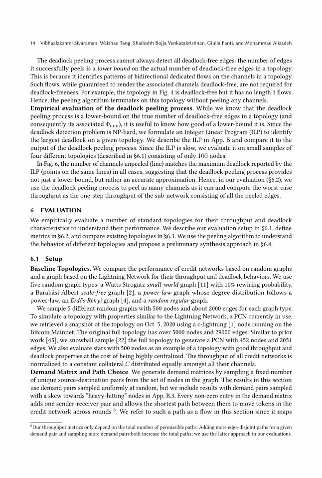
The deadlock peeling process cannot always detect all deadlock-free edges: the number of edgesit successfully peels is a lower bound on the actual number of deadlock-free edges in a topology.This is because it identifies patterns of bidirectional dedicated flows on the channels in a topology.Such flows, while guaranteed to render the associated channels deadlock-free, are not required fordeadlock-freeness. For example, the topology in Fig. 4 is deadlock-free but it has no length 1 flows.Hence, the peeling algorithm terminates on this topology without peeling any channels.Empirical evaluation of the deadlock peeling process. While we know that the deadlockpeeling process is a lower-bound on the true number of deadlock-free edges in a topology (andconsequently its associated Φmin), it is useful to know how good of a lower-bound it is. Since thedeadlock detection problem is NP-hard, we formulate an Integer Linear Program (ILP) to identifythe largest deadlock on a given topology. We describe the ILP in App. B and compare it to theoutput of the deadlock peeling process. Since the ILP is slow, we evaluate it on small samples offour different topologies (described in §6.1) consisting of only 100 nodes.

In Fig. 6, the number of channels unpeeled (line) matches the maximum deadlock reported by theILP (points on the same lines) in all cases, suggesting that the deadlock peeling process providesnot just a lower-bound, but rather an accurate approximation. Hence, in our evaluation (§6.2), weuse the deadlock peeling process to peel as many channels as it can and compute the worst-casethroughput as the one-step throughput of the sub-network consisting of all the peeled edges.

6 EVALUATIONWe empirically evaluate a number of standard topologies for their throughput and deadlockcharacteristics to understand their performance. We describe our evaluation setup in §6.1, definemetrics in §6.2, and compare existing topologies in §6.3. We use the peeling algorithm to understandthe behavior of different topologies and propose a preliminary synthesis approach in §6.4.

6.1 SetupBaseline Topologies. We compare the performance of credit networks based on random graphsand a graph based on the Lightning Network for their throughput and deadlock behaviors. We usefive random graph types: a Watts Strogatz small-world graph [11] with 10% rewiring probability,a Barabási-Albert scale-free graph [2], a power-law graph whose degree distribution follows apower-law, an Erdős-Rényi graph [4], and a random regular graph.

We sample 5 different random graphs with 500 nodes and about 2000 edges for each graph type.To simulate a topology with properties similar to the Lightning Network, a PCN currently in use,we retrieved a snapshot of the topology on Oct. 5, 2020 using a c-lightning [1] node running on theBitcoin Mainnet. The original full topology has over 5000 nodes and 29000 edges. Similar to priorwork [45], we snowball sample [22] the full topology to generate a PCN with 452 nodes and 2051edges. We also evaluate stars with 500 nodes as an example of a topology with good throughput anddeadlock properties at the cost of being highly centralized. The throughput of all credit networks isnormalized to a constant collateral 𝐶 distributed equally amongst all their channels.Demand Matrix and Path Choice. We generate demand matrices by sampling a fixed numberof unique source-destination pairs from the set of nodes in the graph. The results in this sectionuse demand pairs sampled uniformly at random, but we include results with demand pairs sampledwith a skew towards “heavy-hitting” nodes in App. B.3. Every non-zero entry in the demand matrixadds one sender-receiver pair and allows the shortest path between them to move tokens in thecredit network across rounds 6. We refer to such a path as a flow in this section since it maps

6Our throughput metrics only depend on the total number of permissible paths. Adding more edge-disjoint paths for a givendemand pair and sampling more demand pairs both increase the total paths; we use the latter approach in our evaluations.


to a single flow node in the bipartite graph associated with the peeling algorithm. Unlike priorwork [45], we do not explicitly control for a circulation demand since we are interested in theeffect of DAG demands on circulation throughput. As the demand matrix becomes more dense, theamount of circulation demand naturally grows. Unless otherwise mentioned, we sample 4 differentdemand matrices per random instance of the random graphs, to generate 20 unique points overwhich we average the throughput and deadlock behavior. Since there is only one instance of thestar, Lightning Network and our synthesized topology, we use 20 different demand matrices instead.We only present results for demand density ranges that shows variation between the topologies. Ifthe demand matrix is too sparse, there is not enough demand for any topology to perform well; ifit is too dense, just routing one-hop demands (between end-points of every edge in the network)uses all the available collateral in the credit network (Φmax = Φmin = 1).

6.2 MetricsMaximum Throughput. We first compute the maximum per-epoch throughput Φmax that a topol-ogy achieves when none of its channels are imbalanced or constrained. Recall that the throughputof a credit network is maximized at its perfect balance state 𝑪/2. Further, Φmax = 𝜓 (𝑪/2). We usean LP solver to compute𝜓 based on the constrained optimization problem in Eq. 10.Worst-case Throughput. The worst-case throughput of a credit network Φmin is the minimumsteady-state throughput achievable in an epoch from any state in its balance polytope 7. We knowfrom Theorem. 2 that Φmin is achieved at the state with the largest deadlock . Though detectingdeadlocked states on an arbitrary topology is NP-hard, we use our approximate deadlock peelingprocess (§5.2) to identify the deadlock-free channels and compute the worst-case throughput Φmin

as𝜓 (𝑪 ′/2) where 𝑪 ′𝑖 = 𝑪𝑖 if 𝑖 is reported as a deadlock-free channel, and 𝑪 ′𝑖 = 0 otherwise.Fraction of Channels Unpeeled. In addition to the above throughput metrics, we also report thefraction of the channels in the topology that the deadlock peeling process fails to peel. This acts asan upper-bound for the true number of deadlocked channels in a given topology.

6.3 Performance of Random TopologiesFig. 7 shows the best-case throughput Φmax and the worst-case throughput Φmin achievable acrossall starting balance states for a set of random topologies with 500 nodes and an LN topologywith 452 nodes for a fixed collateral budget for 2500–25000 demand pairs sampled uniformly atrandom. Stars outperform all the other topologies by over 50% even at the midpoint of the range.However, stars are highly centralized topologies (i.e., the hub has degree 𝑛); consequently, they areundesirable for decentralized use cases of credit networks. The Φmax value is comparable acrossmost topologies; the small-world topology alone stands as an outlier because it has 50% longerpaths than other topologies which results in lower throughput.Fig. 7 also shows the variation in the Φmin values and the fraction of unpeeled channels across

topologies. For instance, we notice that the Lightning Network, power-law and scale-free topologieshave much better Φmin with fewer flows when compared to the other random graphs suggestingthat they exhibit less throughput sensitivity to the channel balance state. At 7500 demand pairs,both Lightning Network and scale-free topologies peel 20-70% more channels than the small-world,Erdős-Rényi, and random regular topologies and correspondingly have 7-9x higher Φmin. However,the hardship that the scale-free graph faces in peeling the last 10% of its channels manifests as a12% hit to its Φmin when compared to the Lightning Network, particularly with a denser demand

7Our definitions of Φmax and Φmin assume the ability to send the maximum feasible amount between a sender-receiverpair using an ideal routing algorithm. This allows us to reason about throughput without concerning ourselves with theprecise dynamics of any routing algorithm such as transaction sizes or splitting.


●

●● ● ● ● ● ● ● ● ●

●● ● ● ● ● ● ● ● ●

● ● ● ● ● ● ● ● ● ●

Fig. 7. Maximum (Φmax) and minimum throughput (Φmin) achieved by different topologies and channelsleft unpeeled as the number of flows is varied. Stars outperform all other topologies but are undesirable dueto their centralization. The Lightning Network, power-law and scale-free graphs are less sensitive than theother topologies: they peel earlier and have higher Φmin. The fraction of channels peeled corresponds wellwith Φmin: topologies that peel well have a higher Φmin. Whiskers denote max and min data point.

Fig. 8. Evolution of ripple size during the deadlock peeling process on different topologies. At 7500 flows,the ripples of Erdős-Rényi and random regular vanish too quickly preventing them from progressing at allin contrast to Lightning Network, power-law and scale-free topologies. However, while Lightning Network,power-law and scale-free topologies experience good growth at the beginning, they are unable to sustain agood ripple size resulting in the last 6-7% of channels left unprocessed even at 10000 flows.

matrix. This effect is even more pronounced in the power-law graph. In contrast, the Erdős-Rényiand random regular topologies do not peel as well with fewer flows, but quickly improve to peelall channels, on average, with 12500 demands. Beyond this point, their Φmin is comparable withthe Lightning Network. The small-world topology peels only 50% of the flows even with 12500demands which when compounded with its long paths leads to very low Φmin over the entire range.Fig. 13 in App. B.3 shows similar trends across topologies even when demand matrices are skewedin that some “heavy-hitter” nodes are more likely to both send and receive transactions.Explaining the relative behavior of topologies. Given the apparent correlation between Φmin

and the fraction of channels peeled, we now consider the effect of topology on the evolution of thedeadlock peeling process. Fig. 8 shows the evolution of the ripple size at 7500 and 10000 demandpairs, along with the path length distributions for the random regular, Erdős-Rényi, LightningNetwork, power-law and scale-free topologies. We consider the total number of symbols at thestart to be twice the number of channels in the topology, one for each direction of a channel. Eachpeeling step involves processing one channel in one of the two directions. A processed symbol maylead to the release of some flow nodes and consequently, add more directed channels to the ripple.

In Fig. 8, all topologies start with similar initial ripple sizes because they have the same sparsity.In other words, a randomly sampled demand is equally likely to be of length 1 (span only one


edge) across all topologies. However, their ripple evolution patterns quickly diverge. The LightningNetwork, power-law and scale-free topologies experience fast initial ripple growth, attributed tothe 20% degree 2 flows (with path length 2) and up to 60% flows of degree 3. These short flows arelikely to be released early, helping the deadlock peeling process pick up a robust ripple size. Incontrast, at 7500 demands, the ripple vanishes quickly for the random regular and Erdős-Rényitopologies due to 10% fewer degree 2 flows. Yet, the ripples in Lightning Network, power-law andscale-free topologies vanish before the entire topology is peeled, with 250 and 500 directed channelsrespectively unpeeled. This behavior happens with 10000 demands too, albeit to a lesser extent.However, at 10000 flows, Erdős-Rényi and random regular topologies offset the initial dip in theripple size compared to the remaining topologies; they experience later peaks, but peel the entiretopology. The poor tail behavior of the scale-free topology can be attributed to its 6% less channelcoverage for the same number of demand pairs: the presence of hubs means edges far away fromthe hub tend to be less used. Such channels are difficult to peel without a large increase in thenumber of flows that ensures the relevant edges see enough token movement. A similar analysis ofthe ripple evolution for flows sampled in a skewed manner is shown in Fig. 14 in App. B.3.Predicting Performance using LT Codes. Since the deadlock peeling process was inspired bythe design on LT Codes, we evaluate whether the analysis of LT Codes predicts the performanceof the deadlock peeling process. We use the same 5 random graphs from Fig. 8 at 7500 flowsand view their predicted ripple evolution in an LT code with the same degree distribution. Thepredicted ripple evolution computes the probability that a flow of degree 𝑑 is released and addsa symbol to the ripple when there are 𝐿 unprocessed symbols remaining. Extending this to theexpected ripple addition at every step helps build a ripple evolution curve prediction (Eq. 6 of [36]) 8.

Fig. 9. Ripple size predicted by the LT codes anal-ysis on different random topologies at 7500 flows.The prediction suggests that Erdős-Rényi and ran-dom regular ripple sizes dip to zero early on whileLightning Network, power-law and scale-free ex-perience big growths. However, it departs fromthe real ripple size significantly towards the endof the peeling process.

We notice in Fig. 9 that the prediction forthe Lightning Network, power-law and scale-freetopologies are closer to each other but different fromthe Erdős-Rényi and random regular graphs. Like thereal ripple evolution (Fig. 8), the initial growth ratefor the Lightning Network, power-law and scale-freetopologies is faster than the other two graphs. Inter-estingly, the prediction suggests that Erdős-Rényiand random regular topologies will have difficultypeeling at 7500 flows: the predicted ripple sizes ap-proach 0 with around 3000 unprocessed symbolsremaining. Such a ripple evolution is not robust tothe variance encountered during a typical peelingprocess as we observe in Fig. 8 where the rippledecreases drastically early on and vanishes. The pre-diction is more optimistic than the real evolution:the peak ripple sizes are higher and all topologiespeel all their edges. In reality, the deadlock peelingprocess does not peel all the edges even in the Light-ning Network, power-law and scale-free topologies. This difference is anticipated since the LTCodes analyses [26, 36] rely on an i.i.d. bipartite encoding graph where flows (encoded symbols)choose channels (input symbols) uniformly at random. On real graphs, the channels traversed by

8The trajectories use a slightly different expression (Eq. 22) for the expected symbols added that accounts for overlapsbetween symbols covered by the release of different flows at the same step.


flows are correlated; in fact, correlation between edges of flows makes it very hard to peel the last6% of channels in the scale-free topology. Further, we found that with a skewed demand matrix, thecorrelations become stronger and the predictions made using the i.i.d. bipartite graph model deviatefrom reality more significantly (Fig. 14). Hence, a full analysis of the deadlock peeling processshould take into account correlations induced by the topology structure and demand pattern (weleave this to future work). As a first step to understanding the value of such an analysis, we nextinvestigate whether the LT code analysis can be used to synthesize good topologies for uniformrandom demand matrices, where fortuitously LT code predictions are reasonably accurate.

6.4 Topology SynthesisGenerating a path length distribution. Our goal is to find topologies that require fewer demandpairs to render a topology deadlock-free. We start with an approach for LT Codes [36], which fixes adesired ripple evolution and numerically computes a degree distribution that closely approximatesit. In our setting, the degree distribution corresponds to a distribution over path lengths in the creditnetwork. Like [36], we choose a ripple evolution of the form 𝑅(𝐿) = 1.7𝑐1/2.5 where 𝐿 is the numberof unprocessed symbols and 𝑅(𝐿) is the ripple size when 𝐿 symbols remain unprocessed. For atarget graph with 300 nodes and 1500 edges, this ensures a ripple of 30 at the start of the peelingalgorithm, decaying slowly to 25 halfway and eventually to 2 towards the end of the algorithm.

Fig. 10. Desired path length distribution vs.synthesized topology’s distribution.

Next, we choose a path length distribution for the topol-ogy that achieves the desired ripple evolution. Prior workshows that the expected number of symbols added to theripple at each LT process step is a linear function of thepath length distribution [36]. The linear transformationsand constants correspond to the release probabilities andthe desired ripple addition at each step of the algorithmrespectively. For completeness, we outline the equationsin App. B.4.3. We minimize the ℓ2-norm of the differencebetween the expected and desired ripple size. Since ourdegree distributions map to paths on a graph, we con-strain the maximum path length and bound path lengthprobabilities based on the maximum node degree (to en-force decentralization). We also ensure that the numberof length 1 paths does not exceed the number of edges and that the path length probabilities decreasefrom length 2 onwards. Solving this least-squares optimization problem with linear constraintsyields a path length distribution.Synthesizing a matching topology. There are potentially many ways to synthesize a topologywith a given shortest-path length distribution. Our approach exploits a known link between thedistribution of shortest path lengths for a random graph and its pairwise joint degree distribu-tion [33, 46].9 We first set up an optimization using MATLAB to generate a joint degree distributionwhose path length distribution minimizes the ℓ2-norm of the distance from the target path lengthdistribution (output from the previous subsection). Given a joint degree distribution, we use estab-lished methods to generate a random graph that matches the joint degree distribution [5, 20]. Thisapproach is more expressive than the well-known configurationmodel [18], and can (approximately)recover Erdős-Rényi, scale-free, small-world and random regular graphs.

9The pairwise joint degree distribution of a graph evaluated at 𝑗 and ℓ specifies the probability that a randomly samplededge connects nodes of degree 𝑗 and ℓ .


●

●●

●

●

●

●

●

●

●

●

●

●

●

●

● ● ● ●●

●

●

●

●

●

●

●

●

●

● ● ● ●

●

●

●

●

●

●

●

●●

●

Fig. 11. Throughput comparison between a synthesized topology with 271 nodes and its random counterpartsat 300 nodes and 1500 edges. The synthesized topology has lower throughput sensitivity than the randomregular graph and better overall throughput than the scale-free graph. Whiskers denote max and min points.

Results. Our target topology has 300 nodes and 1500 edges. We first use the numerical optimizer tofind a path length distribution that peels well. We observe that permitting a large maximum nodedegree generates path length distributions that the downstream MATLAB optimization routinefails to match well, generating graphs with only 60% of the desired edges. Thus, we ensure that themaximum node degree is 10 and no path is longer than 10 edges. The output distribution from thenumerical optimizer is shown in Fig. 10. When using the MATLAB optimization routine to generatea joint degree distribution, we observe that setting the maximum node degree to 20, average degreeto 10, and maximum path length to 10 ensures a close match to the desired path length distributionwhile avoiding extremely long paths during the synthesis step. We then synthesize a graph with thedesired node distribution and take its largest connected component. The resulting topology has 271nodes and 1513 channels, and achieves a path length distribution close to the one desired (Fig. 10).To evaluate how well the synthesized topology performs, we compare it to 5 instances of randomregular and scale-free topologies with 300 nodes and about 1500 channels in Fig. 11. The maximumthroughput Φmax achieved by the synthesized topology is comparable to the random regular graphand up to 15% better than the scale-free graph, particularly with more demand pairs. The Φmin

and the fraction of channels unpeeled of the synthesized topology strikes a balance between therandom regular and scale-free graphs. It is less sensitive than the random regular topology, notablywith fewer demand pairs, achieving better 10–20% better Φmin and peeling 25–50% more channels.While it is more sensitive than the scale-free graph with sparser demand, it compensates with a15% larger Φmin at denser demands. This approach shows promise in generating topologies thatshow good peeling properties and throughput insensitivity. We leave it to future work to exploregeneralizing this to different demand models to generate even better topologies.Remark. While the above synthesis shows promise, most credit networks are formed by individualnodes’ connectivity decisions, rather than by a centralized authority. However, router nodes incredit networks are incentivized to support high throughput via routing fees, and some PCNsalready include peer recommendation systems that suggest peers to connect to [9, 10]. While weleave the details to future work, we envision building on these systems to encourage desirabletopologies. For example, a credit network software client could “score", or suggest, peers such thatthe overall topology obeys a given joint degree distribution.

7 RELATEDWORKNetwork Topology Design. The peer-to-peer networking literature [25] has studied the design ofstructured [32, 38, 47] and unstructured topologies [3, 24], particularly for efficient content-retrieval.Meanwhile, fat tree [12], Clos [21], small world [41], and random graph [43] topologies have beendesigned to maximize throughput in datacenters. Adapting these ideas to credit networks is hard


due to their centralization—e.g., in a fat tree [12] with 𝑛 top-of-rack (ToR) switches, the aggregationand core switches require a degree of 𝑂 (𝑛1/3).Credit Network Performance. There has been substantial recent interest in quantifying creditnetwork performance, broadly defined as transaction throughput or success rate; prior work hasstudied the impact of several categories of influencing factors, including routing and schedulingprotocols [31, 44, 45, 51, 52], privacy constraints [30, 40, 48, 49], defaulting agents [37], and networktopology [13, 15, 16, 23]. Prior work exploring the effects of credit network topology on transactionsuccess rate [15] assumed sequential transactions and a full demandmatrix. In this setting, maximumthroughput can be trivially achieved with length-1 flows, so no deadlocks are observed.

Demand-aware design of payment channel network topologies [16] poses the problem as an ILP:given a channel budget, a set of nodes, and a demand matrix, the ILP finds an adjacency matrix thateither maximizes the number of connected demand pairs [13] or minimizes the number of channelsadded and the average path length [23]. This approach ignores the effects of channel imbalance,which causes the deadlock-related problems explored in this work.Erasure Codes. Sparse graph codes have been studied for decades in channel coding [14, 19, 26–28, 39, 42]. We identify a parallel between such codes and detecting deadlocked edges in a topology.However, despite a rich literature on sparse graph codes, our setting cannot fully utilize mostexisting constructions for two reasons. First, we need to be able to change the number of flows(encoding symbols) flexibly, without requiring a totally new encoding. We therefore use ratelesscodes [26, 27, 42]; specifically, our peeling algorithm builds closely on Luby’s LT codes [26]. Second,our encoding procedure must respect the topology constraints of the underlying graph; we cannotassign channels uniformly at random to flows, as in classical sparse graph codes. To our knowledge,this constraint has not been previously studied. This is why our theoretical predictions for thenumber of flows needed to peel a graph (from [26]) are lower than the number needed in practice(§6). More broadly, this suggests an interesting direction of further study on error-correcting codesthat obey encoding constraints imposed by a graph topology.

8 CONCLUSIONIn this paper, we studied the effects of topology and channel imbalance on the throughput of creditnetworks. We demonstrated a close relation between worst-case throughput and the presence ofdeadlocks, and proposed a heuristic peeling algorithm for identifying the presence of deadlocks.Important directions for future work include synthesizing graphs that are: (a) easy to peel, (b) exhibithigh throughput, and (c) limit the maximum degree of any node. While we have made progress onthat front, we were not able to find topologies that perform substantially better than random graphs.Hence, an interesting question is whether this is even possible. Another interesting direction is toanalyze the peeling algorithm given the correlations induced (in the bipartite graph) by an arbitrarytopology and demand pattern. Further, this work assumes perfect routing; in practice it is unclearwhether one can actually achieve 𝜙 (𝒃). Designing decentralized routing protocols that are tailoredto good credit network topologies and understanding their performance with respect to theseupper bounds will be important in practice. Finally, designing suitable incentive/recommendationmechanisms to achieve a desired topology in a decentralized manner is an important problem.

ACKNOWLEDGMENTSWe thank our anonymous reviewers for their detailed feedback. This work was supported in partby an AFOSR grant FA9550-21-1-0090; NSF grants CNS-1751009, CNS-1910676, and CIF-1705007;a Microsoft Faculty Fellowship; awards from the Cisco Research Center and the Fintech@CSAILprogram; and gifts from Chainlink, the Sloan Foundation, and the Ripple Foundation.


REFERENCES[1] [n.d.]. Amount-independent payment routing in Lightning Networks. https://medium.com/coinmonks/amount-

independent-payment-routing-in-lightning-networks-6409201ff5ed.[2] [n.d.]. Barabási-Albert Graph. https://networkx.github.io/documentation/networkx-1.9.1/reference/generated/

networkx.generators.random_graphs.barabasi_albert_graph.html.[3] [n.d.]. BitTorrent. https://www.bittorrent.com.[4] [n.d.]. Erdős-Rényi Graph. https://networkx.org/documentation/stable//reference/generated/networkx.generators.

random_graphs.erdos_renyi_graph.html.[5] [n.d.]. Joint-Degree Graph. https://networkx.org/documentation/stable/reference/generated/networkx.generators.

joint_degree_seq.joint_degree_graph.html.[6] [n.d.]. Joint-Degree Graph Validation. https://networkx.org/documentation/stable/reference/generated/networkx.

generators.joint_degree_seq.is_valid_joint_degree.html.[7] [n.d.]. MATLAB optimizer. https://www.mathworks.com/help/optim/ug/fmincon.html.[8] [n.d.]. Raiden Network. https://raiden.network/.[9] [n.d.]. The Node Operator’s Guide to the Lightning Galaxy, Part 1. https://lightning.engineering/posts/2019-07-30-

routing-quide-1/.[10] [n.d.]. The Node Operator’s Guide to the Lightning Galaxy, Part 2: Node Scoring and Pathfinding. https://lightning.

engineering/posts/2019-11-07-routing-guide-2/.[11] [n.d.]. Watts-Strogatz Graph. https://networkx.github.io/documentation/networkx-1.9/reference/generated/networkx.

generators.random_graphs.watts_strogatz_graph.html.[12] Mohammad Al-Fares, Alexander Loukissas, and Amin Vahdat. 2008. A scalable, commodity data center network

architecture. ACM SIGCOMM computer communication review 38, 4 (2008), 63–74.[13] Lukas Aumayr, Esra Ceylan, Matteo Maffei, Pedro Moreno-Sanchez, Iosif Salem, and Stefan Schmid. 2020. Demand-

Aware Payment Channel Networks. arXiv preprint arXiv:2011.14341 (2020).[14] John W Byers, Michael Luby, Michael Mitzenmacher, and Ashutosh Rege. 1998. A digital fountain approach to reliable

distribution of bulk data. ACM SIGCOMM Computer Communication Review 28, 4 (1998), 56–67.[15] Pranav Dandekar, Ashish Goel, Ramesh Govindan, and Ian Post. 2011. Liquidity in credit networks: A little trust goes

a long way. In Proceedings of the 12th ACM conference on Electronic commerce. 147–156.[16] Pranav Dandekar, Ashish Goel, Michael P Wellman, and Bryce Wiedenbeck. 2015. Strategic formation of credit

networks. ACM Transactions on Internet Technology (TOIT) 15, 1 (2015), 1–41.[17] Christian Decker and RogerWattenhofer. 2015. A fast and scalable payment network with bitcoin duplex micropayment

channels. In Symposium on Self-Stabilizing Systems. Springer, 3–18.[18] Bailey K Fosdick, Daniel B Larremore, Joel Nishimura, and Johan Ugander. 2018. Configuring random graph models

with fixed degree sequences. Siam Review 60, 2 (2018), 315–355.[19] Robert Gallager. 1962. Low-density parity-check codes. IRE Transactions on information theory 8, 1 (1962), 21–28.[20] Minas Gjoka, Bálint Tillman, and Athina Markopoulou. 2015. Construction of simple graphs with a target joint degree

matrix and beyond. In 2015 IEEE Conference on Computer Communications (INFOCOM). IEEE, 1553–1561.[21] Albert Greenberg, James R Hamilton, Navendu Jain, Srikanth Kandula, Changhoon Kim, Parantap Lahiri, David A

Maltz, Parveen Patel, and Sudipta Sengupta. 2009. VL2: A scalable and flexible data center network. In Proceedings ofthe ACM SIGCOMM 2009 conference on Data communication. 51–62.

[22] Pili Hu and Wing Cheong Lau. 2013. A survey and taxonomy of graph sampling. arXiv preprint arXiv:1308.5865 (2013).[23] Julia Khamis and Ori Rottenstreich. [n.d.]. Demand-aware Channel Topologies for Off-chain Blockchain Payments.

([n. d.]).[24] Joohwan Kim and Rayadurgam Srikant. 2013. Real-time peer-to-peer streaming over multiple random hamiltonian

cycles. IEEE transactions on information theory 59, 9 (2013), 5763–5778.[25] Eng Keong Lua, Jon Crowcroft, Marcelo Pias, Ravi Sharma, and Steven Lim. 2005. A survey and comparison of

peer-to-peer overlay network schemes. IEEE Communications Surveys & Tutorials 7, 2 (2005), 72–93.[26] Michael Luby. 2002. LT codes. In The 43rd Annual IEEE Symposium on Foundations of Computer Science, 2002. Proceedings.

IEEE, 271–280.[27] Michael G Luby, Michael Mitzenmacher, Mohammad Amin Shokrollahi, and Daniel A Spielman. 2001. Efficient erasure

correcting codes. IEEE Transactions on Information Theory 47, 2 (2001), 569–584.[28] David JC MacKay. 1999. Good error-correcting codes based on very sparse matrices. IEEE transactions on Information

Theory 45, 2 (1999), 399–431.[29] Mr Samuel Munzele Maimbo, Mr Mohammed El Qorchi, and Mr John F Wilson. 2003. Informal Funds Transfer Systems:

An analysis of the informal hawala system. International Monetary Fund.[30] Giulio Malavolta, Pedro Moreno-Sanchez, Aniket Kate, and Matteo Maffei. 2017. SilentWhispers: Enforcing Security

and Privacy in Decentralized Credit Networks.. In NDSS.

https://medium.com/coinmonks/amount-independent-payment-routing-in-lightning-networks-6409201ff5ed

https://medium.com/coinmonks/amount-independent-payment-routing-in-lightning-networks-6409201ff5ed

https://networkx.github.io/documentation/networkx-1.9.1/reference/generated/networkx.generators.random_graphs.barabasi_albert_graph.html

https://networkx.github.io/documentation/networkx-1.9.1/reference/generated/networkx.generators.random_graphs.barabasi_albert_graph.html

https://www.bittorrent.com

https://networkx.org/documentation/stable//reference/generated/networkx.generators.random_graphs.erdos_renyi_graph.html

https://networkx.org/documentation/stable//reference/generated/networkx.generators.random_graphs.erdos_renyi_graph.html

https://networkx.org/documentation/stable/reference/generated/networkx.generators.joint_degree_seq.joint_degree_graph.html

https://networkx.org/documentation/stable/reference/generated/networkx.generators.joint_degree_seq.joint_degree_graph.html

https://networkx.org/documentation/stable/reference/generated/networkx.generators.joint_degree_seq.is_valid_joint_degree.html

https://networkx.org/documentation/stable/reference/generated/networkx.generators.joint_degree_seq.is_valid_joint_degree.html

https://www.mathworks.com/help/optim/ug/fmincon.html

https://raiden.network/

https://lightning.engineering/posts/2019-07-30-routing-quide-1/

https://lightning.engineering/posts/2019-07-30-routing-quide-1/

https://lightning.engineering/posts/2019-11-07-routing-guide-2/

https://lightning.engineering/posts/2019-11-07-routing-guide-2/

https://networkx.github.io/documentation/networkx-1.9/reference/generated/networkx.generators.random_graphs.watts_strogatz_graph.html

https://networkx.github.io/documentation/networkx-1.9/reference/generated/networkx.generators.random_graphs.watts_strogatz_graph.html


[31] Giulio Malavolta, Pedro Moreno-Sanchez, Aniket Kate, Matteo Maffei, and Srivatsan Ravi. 2017. Concurrency andprivacy with payment-channel networks. In Proceedings of the 2017 ACM SIGSAC Conference on Computer and Commu-nications Security. 455–471.

[32] Petar Maymounkov and David Mazieres. 2002. Kademlia: A peer-to-peer information system based on the xor metric.In International Workshop on Peer-to-Peer Systems. Springer, 53–65.

[33] Sergey Melnik and James P Gleeson. 2016. Simple and accurate analytical calculation of shortest path lengths. arXivpreprint arXiv:1604.05521 (2016).

[34] Pedro Moreno-Sanchez, Navin Modi, Raghuvir Songhela, Aniket Kate, and Sonia Fahmy. 2018. Mind your credit:Assessing the health of the ripple credit network. In Proceedings of the 2018 World Wide Web Conference. 329–338.

[35] Joseph Poon and Thaddeus Dryja. 2016. The Bitcoin Lightning Network: Scalable Off-chain Instant Payments. draftversion 0.5 9 (2016), 14.

[36] Petar Popovski, Jan Ostergaard, et al. 2012. Design and analysis of LT codes with decreasing ripple size. IEEETransactions on Communications 60, 11 (2012), 3191–3197.

[37] Geoffrey Ramseyer, Ashish Goel, and David Mazières. 2020. Liquidity in credit networks with constrained agents. InProceedings of The Web Conference 2020. 2099–2108.

[38] Sylvia Ratnasamy, Paul Francis, Mark Handley, Richard Karp, and Scott Shenker. 2001. A scalable content-addressablenetwork. In Proceedings of the 2001 conference on Applications, technologies, architectures, and protocols for computercommunications. 161–172.

[39] Thomas J Richardson, Mohammad Amin Shokrollahi, and Rüdiger L Urbanke. 2001. Design of capacity-approachingirregular low-density parity-check codes. IEEE transactions on information theory 47, 2 (2001), 619–637.

[40] Stefanie Roos, Pedro Moreno-Sanchez, Aniket Kate, and Ian Goldberg. 2017. Settling payments fast and private:Efficient decentralized routing for path-based transactions. arXiv preprint arXiv:1709.05748 (2017).

[41] Ji-Yong Shin, Bernard Wong, and Emin Gün Sirer. 2011. Small-world datacenters. In Proceedings of the 2nd ACMSymposium on Cloud Computing. 1–13.

[42] Amin Shokrollahi. 2006. Raptor codes. IEEE transactions on information theory 52, 6 (2006), 2551–2567.[43] Ankit Singla, Chi-Yao Hong, Lucian Popa, and P Brighten Godfrey. 2012. Jellyfish: Networking data centers randomly.

In 9th {USENIX} Symposium on Networked Systems Design and Implementation ({NSDI} 12). 225–238.[44] Vibhaalakshmi Sivaraman, Shaileshh Bojja Venkatakrishnan,MohammadAlizadeh, Giulia Fanti, and PramodViswanath.

2018. Routing Cryptocurrency with the Spider Network. In Proceedings of the 17th ACM Workshop on Hot Topics inNetworks. ACM, 29–35.

[45] Vibhaalakshmi Sivaraman, Shaileshh Bojja Venkatakrishnan, Kathleen Ruan, Parimarjan Negi, Lei Yang, RadhikaMittal, Giulia Fanti, and Mohammad Alizadeh. 2020. High Throughput Cryptocurrency Routing in Payment ChannelNetworks. In 17th {USENIX} Symposium on Networked Systems Design and Implementation ({NSDI} 20). 777–796.

[46] Isabelle Stanton and Ali Pinar. 2012. Constructing and sampling graphs with a prescribed joint degree distribution.Journal of Experimental Algorithmics (JEA) 17 (2012), 3–1.

[47] Ion Stoica, Robert Morris, David Karger, M Frans Kaashoek, and Hari Balakrishnan. 2001. Chord: A scalable peer-to-peerlookup service for internet applications. ACM SIGCOMM Computer Communication Review 31, 4 (2001), 149–160.

[48] Weizhao Tang, Weina Wang, Giulia Fanti, and Sewoong Oh. 2020. Privacy-utility tradeoffs in routing cryptocurrencyover payment channel networks. Proceedings of the ACM on Measurement and Analysis of Computing Systems 4, 2(2020), 1–39.

[49] Sergei Tikhomirov, Pedro Moreno-Sanchez, and Matteo Maffei. 2020. A quantitative analysis of security, anonymity andscalability for the lightning network. In 2020 IEEE European Symposium on Security and Privacy Workshops (EuroS&PW).IEEE, 387–396.

[50] Kyle Torpey. 2016. Greg Maxwell: Lightning Network Better Than Sidechains for Scaling Bitcoin. https://bitcoinmagazine.com/articles/greg-maxwell-lightning-network-better-than-sidechains-for-scaling-bitcoin-1461077424/.

[51] Peng Wang, Hong Xu, Xin Jin, and Tao Wang. 2019. Flash: efficient dynamic routing for offchain networks. InProceedings of the 15th International Conference on Emerging Networking Experiments And Technologies. 370–381.

[52] Shira Werman and Aviv Zohar. 2018. Avoiding deadlocks in payment channel networks. In Data Privacy Management,Cryptocurrencies and Blockchain Technology. Springer, 175–187.

https://bitcoinmagazine.com/articles/greg-maxwell-lightning-network-better-than-sidechains-for-scaling-

https://bitcoinmagazine.com/articles/greg-maxwell-lightning-network-better-than-sidechains-for-scaling-

bitcoin-1461077424/


A THEORETICAL RESULTSA.1 Basic Properties

Proposition 4. For any state 𝒃 , X𝒃 is a convex set and 𝒃 ∈ X𝒃 .

Proposition 5. For a balance state 𝒃 ∈ R |𝐸 |≥0, if 𝒙,𝒚 ∈ D𝒃 , then 𝛼𝒙 + 𝛽𝒚 ∈ D𝒃 for any 𝛼, 𝛽 ∈ R≥0.

Proposition 6. For any 𝒇 : 𝒇 ≥ 0 and 𝑅𝒇 ≤[

𝒃𝑪 − 𝒃

], we have 𝒃 − Δ𝑅𝒇 ∈ X𝒃 and 𝒇 ∈ F𝒃 .

Proposition 7. 𝒃 ∈ X𝒂 ⇐⇒ X𝒃 ⊆ X𝒂 .

Proposition 8. The center state has maximized𝜓 . Precisely,𝜓(𝑪

2

)= max𝒂∈B𝜓 (𝒂).

Proposition 9.L𝒃 =

{𝑖 ∈ [|𝐸 |]

�� 𝑎𝑖 = 𝑏𝑖 , ∀𝒂 ∈ X𝒃}

Proposition 10. If 𝑖 ∈ L𝒃 , then for all 𝒇 ∈ F𝒃 whose decomposition is a sequence of flows(𝒇 ( 𝑗)

)𝑘−1𝑗=0

,

we have(1) For all 𝑗 ∈ [𝑘], 𝑅𝑖𝒇 ( 𝑗) = 𝑅

𝑖𝒇 ( 𝑗) = 0;

(2) For all 𝑗 ∈ [𝑘] and 𝜋 ∈ Π (index of path) where 𝑅𝑖,𝜋 = 1 ∨ 𝑅𝑖,𝜋

= 1, 𝒇 ( 𝑗)𝜋 = 0.

A.2 Supporting Theorems

Lemma 11. If for some 𝜖 ≥ 0, 𝜖[

𝒂𝑪 − 𝒂

]≤

[𝒃

𝑪 − 𝒃

], then for all 𝒑 ∈ X𝒂 , we have 𝒃 +𝜖 (𝒑−𝒂) ∈ X𝒃 .

Proof. Since 𝒑 ∈ X𝒂 , ∃𝑘 ∈ N, a sequence of flows 𝒇 (0:𝑘−1) and a sequence of transient states𝒂 (0:𝑘) , where 𝒂 (0) = 𝒂, 𝒂 (𝑘) = 𝒑, and for all 𝑗 ∈ [𝑘],

𝒂 ( 𝑗+1) = 𝒂 ( 𝑗) − Δ𝑅𝒇 ( 𝑗) , 𝒇 ( 𝑗) ≥ 0, 𝑅𝒇 ( 𝑗) ≤[

𝒂 ( 𝑗)

𝑪 − 𝒂 ( 𝑗)].

Consider new flows 𝒈 ( 𝑗) = 𝜖𝒇 ( 𝑗) for 𝜖 ≥ 0 and 𝑗 ∈ [𝑘]. Starting from state 𝒃 (0) = 𝒃 , we send

flows(𝒈 ( 𝑗)

)𝑘−1𝑗=0 and obtain transient states

(𝒃 ( 𝑗)

)𝑘𝑗=0

, where for all 𝑗 ∈ [𝑘],

𝒃 ( 𝑗+1) = 𝒃 ( 𝑗) − Δ𝑅𝒈 ( 𝑗) = 𝒃 ( 𝑗) − 𝜖Δ𝑅𝒇 ( 𝑗) = 𝒃 − 𝜖Δ𝑅𝑗∑︁

𝑖=0

𝒇 (𝑖) = 𝒃 + 𝜖(𝒂 ( 𝑗+1) − 𝒂

).

Note that 𝒃 (0) = 𝒃 + 𝜖0 = 𝒃 + 𝜖(𝒂 (0) − 𝒂

). Staring with 𝜖

[𝒂

𝑪 − 𝒂

]≤

[𝒃

𝑪 − 𝒃

], we have

𝜖

[𝒂

𝑪 − 𝒂

]≤

[𝒃

𝑪 − 𝒃

]=⇒ 𝜖

[𝒂 ( 𝑗)

𝑪 − 𝒂 ( 𝑗)]≤

[𝒃

𝑪 − 𝒃

]+ 𝜖

( [𝒂 ( 𝑗)

𝑪 − 𝒂 ( 𝑗)]−

[𝒂

𝑪 − 𝒂

] )=

[𝒃 ( 𝑗)

𝑪 − 𝒃 ( 𝑗)], ∀𝑗 ∈ [𝑘]

=⇒ 𝑅𝒈 ( 𝑗) = 𝜖𝑅𝒇 ( 𝑗) ≤ 𝜖

[𝒂 ( 𝑗)

𝑪 − 𝒂 ( 𝑗)]≤

[𝒃 ( 𝑗)

𝑪 − 𝒃 ( 𝑗)], ∀𝑗 ∈ [𝑘] .


Therefore, combining with 𝒈 ( 𝑗) = 𝜖𝒇 ( 𝑗) ≥ 0, we know(𝒈 ( 𝑗)

)𝑘−1𝑗=0 = 𝜖

(𝒇 ( 𝑗)

)𝑘−1𝑗=0

is a valid sequenceof flows that leads to a reachable state from 𝒃 . In other words,

X𝒃 ∋ 𝒃 (𝑘) = 𝒃 − Δ𝑅𝑘−1∑︁𝑗=0

𝒈 ( 𝑗) = 𝒃 − 𝜖Δ𝑅𝑘−1∑︁𝑗=0

𝒇 ( 𝑗) = 𝒃 + 𝜖 (𝒑 − 𝒂). ■

Lemma 12. Let 𝒃 ∈ X𝒂 − {𝒂} and 𝒑 ≜ argmax𝒑′∈B{∥𝒑 ′ − 𝒂∥2 |∃𝑡 ≥ 0 : 𝒑 ′ − 𝒂 = 𝑡 (𝒃 − 𝒂)} be the

intersection with the boundary of state space with the direction along 𝒂 to 𝒃 . Let 𝑟 =∥𝒑 − 𝒃 ∥2∥𝒑 − 𝒂∥2

∈ [0, 1).

For all 𝑡 ∈ [0, 1 − 𝑟2], 𝒂 + 𝑡 (𝒑 − 𝒂) ∈ X𝒂 and for all 𝑡 ∈ [1 − 𝑟, 1 − 𝑟2], 𝒂 + 𝑡 (𝒑 − 𝒂) ∈ X𝒃 .

Proof. By 𝒃 ∈ X𝒂 , there exists a 𝑘 ∈ N, a sequence of flows 𝒇 (0:𝑘−1) and a sequence of transientstates 𝒂 (0:𝑘) , where 𝒂 (0) = 𝒂, 𝒂 (𝑘) = 𝒃 , and for all 𝑗 ∈ [𝑘],

𝒂 ( 𝑗+1) = 𝒂 ( 𝑗) − Δ𝑅𝒇 ( 𝑗) , 𝒇 ( 𝑗) ≥ 0, 𝑅𝒇 ( 𝑗) ≤[

𝒂 ( 𝑗)

𝑪 − 𝒂 ( 𝑗)].

States on segment [𝒂, 𝒃]. These states correspond to 𝑡 ∈ [0, 1 − 𝑟 ].

For any constant 𝜖 ∈ [0, 1], we have 𝜖[

𝒂𝑪 − 𝒂

]≤

[𝒂

𝑪 − 𝒂

]. Citing Lemma 11 and using the fact

that 𝒃 ∈ X𝒂 , we obtain 𝒂 + 𝜖 (𝒃 − 𝒂) ∈ X𝒂 , for all 𝜖 ∈ [0, 1]. From 𝒂 + 𝜖 (𝒃 − 𝒂) = 𝒂 + 𝜖 (1− 𝑟 ) (𝒑 − 𝒂),we know the statement is true for all 𝑡 ∈ [0, 1 − 𝑟 ].

States on segment [𝒃, 𝒄]. These states correspond to 𝑡 ∈ [1 − 𝑟, 1 − 𝑟2], or a part of the segment[𝒃,𝒑].

Starting with 0 ≤ 𝜖 ≤ 𝑟 < 1 and −[

𝒂𝑪 − 𝒂

]≤ 0 ≤

[𝒑

𝑪 − 𝒑

], we have the following deductions.

(0 ≤ 𝜖 ≤ 𝑟 < 1) ∧(−

[𝒂

𝑪 − 𝒂

]≤ 0 ≤

[𝒑

𝑪 − 𝒑

] )=⇒ (𝜖 − 𝑟 )

[𝒂

𝑪 − 𝒂

]≤ 0 ≤ (1 − 𝑟 )

[𝒑

𝑪 − 𝒑

]=⇒ 𝜖

[𝒂

𝑪 − 𝒂

]≤

[𝒑

𝑪 − 𝒑

]− 𝑟

( [𝒑

𝑪 − 𝒑

]−

[𝒂

𝑪 − 𝒂

] )=

[𝒃

𝑪 − 𝒃

].

Citing Lemma 11, we have 𝒃 + 𝜖 (𝒃 − 𝒂) ∈ X𝒃 . By transitivity of reachable states (Prop. 7), wehave for all 𝜖 ∈ [0, 𝑟 ],

X𝒂 ⊇ X𝒃 ∋ 𝒃 + 𝜖 (𝒃 − 𝒂) = 𝒂 + (1 − 𝑟 ) (1 + 𝜖) (𝒑 − 𝒂).In other words, for all 𝑡 ∈ [1 − 𝑟, 1 − 𝑟2], 𝒂 + 𝑡 (𝒑 − 𝒂) ∈ X𝒂 ∩ X𝒃 . The proof is now complete. ■

Theorem 13. Assume 𝝃 ∈ D𝒂 − {0} is a feasible direction and 𝒑 ≜ argmax𝒑′∈B{∥𝒑 ′ − 𝒂∥2 |∃𝑡 ≥0 : 𝒑 ′− 𝒂 = 𝑡𝝃 } is the ray’s last intersection with the state space. For all 𝑡 ∈ [0, 1), 𝒂 + 𝑡 (𝒑 − 𝒂) ∈ X𝒂 .

Proof. By definition of D𝒂 , ∃𝒃 ∈ X𝒂 , 𝑟 ∈ [0, 1), such that 𝒑 − 𝒃 = 𝑟 (𝒑 − 𝒂). If 𝒃 itself is the endpoint on the boundary, then 𝑟 = 0 and𝒑 = 𝒃 . Then, using Lemma 12, we can trivially prove the claim.

If 0 < 𝑟 < 1, we can take 𝑘 = ⌈log𝑟 (1 − 𝑡)⌉ ∈ N which satisfies 1 − 𝑟𝑘 ≥ 𝑡 . Then, we construct asequence of transient states

(𝒂 ( 𝑗)

)𝑘𝑗=0, where 𝒂

( 𝑗) = 𝒂 + (1 − 𝑟 𝑗 ) (𝒑 − 𝒂) for all 𝑗 ∈ [𝑘] ∪ {𝑘}. By


this definition,

𝒂 (0) = 𝒂, 𝒂 (1) = 𝒃, ∀𝑗 ∈ [𝑘] : 𝒑 − 𝒂 ( 𝑗+1) = 𝑟(𝒑 − 𝒂 ( 𝑗)

).

We recursively show 𝒂 ( 𝑗+1) ∈ X𝒂 ( 𝑗 ) for all 𝑗 ∈ [𝑘]. This is true for 𝑗 = 0 given 𝒃 ∈ X𝒂 .Suppose 𝒂 ( 𝑗+1) ∈ X𝒂 ( 𝑗 ) is true for 𝑗 = 𝐽 − 1 < 𝑘 − 1. Then for 𝑗 = 𝐽 , we have

𝒂 ( 𝐽 +1) = 𝒑 − 𝑟(𝒑 − 𝒂 ( 𝐽 )

)= 𝒂 ( 𝐽 −1) + (1 − 𝑟2)

(𝒑 − 𝒂 ( 𝐽 −1)

).

By Lemma 12, combined with 𝒑−𝒂 ( 𝐽 +1) = 𝑟(𝒑 − 𝒂 ( 𝐽 )

)and 𝒂 ( 𝐽 ) ∈ X𝒂 ( 𝐽 −1) , we have 𝒂 ( 𝐽 +1) ∈ X𝒂 ( 𝐽 ) .

Therefore, 𝒂 ( 𝑗+1) ∈ X𝒂 ( 𝑗 ) for all 𝑗 ∈ [𝑘]. By Proposition 7 (transitive reachability), this furtherimplies 𝒂 (𝑘) ∈ X𝒂 . Since

𝒄 ≜ 𝒂 + 𝑡 (𝒑 − 𝒂) = 𝒂 + 𝑡

1 − 𝑟𝑘(𝒂 (𝑘) − 𝒂

),

we know by 𝑡

1 − 𝑟𝑘≤ 1 that 𝒄 is on segment

[𝒂, 𝒂 (𝑘)

]. By Lemma 12, we have 𝒂 + 𝑡 (𝒑 − 𝒂) =

𝒄 ∈ X𝒂 . ■

Corollary 14. If 𝝃 ∈ D𝒂 is a feasible direction, {𝒃 | 𝒃 ∈ B+, ∃𝑡 ≥ 0(𝒃 = 𝒂 + 𝑡𝝃 )} ⊆ X𝒂 .

Lemma 15. For balance states 𝒂, 𝒃 ∈ B, if 𝑍𝒃 ⊆ 𝑍𝒂 , then D𝒂 ⊆ D𝒃 .

Proof. For 𝝃 = 0 ∈ D𝒂 , we trivially obtain that 𝝃 = 0 ∈ D𝒃 .For any 𝝃 ∈ D𝒂 − {0}, there exists 𝑡 > 0 and 𝒑 ∈ X𝒂 , where 𝒑 = 𝒂 + 𝑡𝝃 . Take

𝜖 = min𝑖∉𝑍𝒂

[𝒃

𝑪 − 𝒃

]𝑖[

𝒂𝑪 − 𝒂

]𝑖

.

By 𝑍𝒃 ⊆ 𝑍𝒂 , we have 𝜖 > 0 and 𝜖

[𝒂

𝑪 − 𝒂

]≤

[𝒃

𝑪 − 𝒃

]. By Lemma 11, we have for all 𝒑 ∈ X𝒂 ,

𝒃 + 𝜖𝑡𝝃 = 𝒃 + 𝜖 (𝒑 − 𝒂) ∈ X𝒃 . Given 𝜖𝑡 > 0, we have 𝝃 ∈ D𝒃 . Therefore, D𝒂 ⊆ D𝒃 . ■

Lemma 16. Let 𝜙 (𝒃;Π) denote the throughput starting from initial state 𝒃 under set of feasiblepaths Π. For any state 𝒃 , if Π′ ⊆ Π,

𝜙 (𝒃;Π) ≥ 𝜙 (𝒃;Π′). (13)

Let F𝒃 ⊆ R |Π |, F′𝒃 ⊆ R|Π′ | denote the set of feasible flows from 𝒃 under Π,Π′, respectively. Through-

put equality is attained when all paths in Π − Π′ are unused or in other words, if 𝒇 ∈ F𝒃 , 𝑓𝜋 = 0 holdsfor any 𝜋 ∉ Π′.

Proof. Let X𝒃 ,X′𝒃 denote the set of reachable states from 𝒃 , under feasible paths Π,Π′, withrouting matrices 𝑅, 𝑅′ respectively.Since, Π′ ⊆ Π implies there exists a matrix 𝑃 ∈ {0, 1} |Π |× |Π′ | , such that 𝑅′ = 𝑅𝑃 . Note that everyrow of 𝑃 can have utmost one non-zero entry and every column of 𝑃 has exactly one non-zeroentry. In particular, 𝑃𝑖 𝑗 = 1 if Π𝑖 = Π′𝑗 and 0 otherwise. Consequently, for all 𝒈 ∈ R |Π′ | , there existsan 𝒇 = 𝑃𝒈 ∈ R |Π | satisfying 𝑅𝒇 = 𝑅𝑃𝒈 = 𝑅′𝒈 and Δ𝑅𝒇 = Δ𝑅′𝒈.

Mapping the reachable states.For any 𝒑 ∈ X′𝒃 , there exists a 𝑘 ∈ N, a sequence of flows 𝒈

(0:𝑘−1) and a sequence of transient states


𝒃 (0:𝑘) , where 𝒃 (0) = 𝒃 , 𝒃 (𝑘) = 𝒑, and for all 𝑗 ∈ [𝑘],

𝒃 ( 𝑗+1) = 𝒃 ( 𝑗) − Δ𝑅′𝒈 ( 𝑗) , 𝒈 ( 𝑗) ≥ 0, 𝑅′𝒈 ( 𝑗) ≤[

𝒃 ( 𝑗)

𝑪 − 𝒃 ( 𝑗)].

Now let 𝒇 ( 𝑗) = 𝑃𝒈 ( 𝑗) for each 𝑗 ∈ [𝑘]. We may directly obtain

𝒃 ( 𝑗+1) = 𝒃 ( 𝑗) − Δ𝑅𝒇 ( 𝑗) , 𝒇 ( 𝑗) ≥ 0, 𝑅𝒇 ( 𝑗) ≤[

𝒃 ( 𝑗)

𝑪 − 𝒃 ( 𝑗)].

This implies 𝒇 =∑𝑘−1

𝑗=0 𝑃𝒈( 𝑗) = 𝑃𝒈 is also feasible that leads to a reachable state 𝒑 = 𝒃 − Δ𝑅′𝒈 =

𝒃 − Δ𝑅𝒇 . Hence, 𝒑 ∈ X𝒃 , and since 𝒑 is an arbitrary element in X′𝒃 , we have X𝒃′ ⊆ X𝒃 .Mapping Throughput Functions.For any 𝒈 ∈ R |Π′ | , there exists 𝒇 = 𝑃𝒈 ∈ R |Π | , where 1⊤𝒇 = 1⊤𝑃𝒈 = 1⊤𝒈 and 𝑅𝒇 = 𝑅𝑃𝒈 = 𝑅′𝒈.

Hence,(𝒈 ≥ 0, 𝑅′𝒈 ≤

[𝒃

𝑪 − 𝒃

], Δ𝑅′𝒈 = 0

)=⇒

(𝒇 ≥ 0, 𝑅𝒇 ≤

[𝒃

𝑪 − 𝒃

], Δ𝑅𝒇 = 0

), which further

indicates

Ψ′ ≜

{1⊤𝒈

��𝒈 ≥ 0, 𝑅′𝒈 ≤[

𝒃𝑪 − 𝒃

], Δ𝑅′𝒈 = 0

}⊆

{1⊤𝒇

��𝒇 ≥ 0, 𝑅𝒇 ≤[

𝒃𝑪 − 𝒃

], Δ𝑅𝒇 = 0

}≜ Ψ.

Let𝜓 (𝒂; Π̃) denote the one-step maximum throughput at state 𝒂 under arbitrary set of feasibleflows Π̃. By definition of𝜓 , we have

𝜓 (𝒂;Π) = supΨ ≥ supΨ′ = 𝜓 (𝒂;Π′).

Equality Case. Assume for any feasible flow 𝒇 ∈ F𝒃 , 𝑓𝜋 = 0 holds for any 𝜋 ∉ Π′. Based on theconstruction of 𝑃 , (𝑃𝑃⊤)𝜋,𝜋 = 0 if 𝜋 ∉ Π′ and (𝑃𝑃⊤)𝜋,𝜋 = 1 if 𝜋 ∈ Π′ . So, for this special case, wecan argue 𝑃𝑃⊤𝒇 = 𝒇 .Let 𝒑 be an arbitrary state in X𝒃 . Then, there exists 𝒇 ∈ F𝒃 such that 𝒑 = 𝒃 − Δ𝑅𝒇 . Construct

𝒈 = 𝑃⊤𝒇 , such that −Δ𝑅′𝒈 = −Δ𝑅𝑃𝑃⊤𝒇 = −Δ𝑅𝒇 . 𝒈 ∈ F′𝒃 . Similar to the previous argument,𝒑 = 𝒃 − Δ𝑅𝒇 = 𝒃 − Δ𝑅′𝒈 ∈ X′𝒃 . Thus, X𝒃 ⊆ X

′𝒃 . This, with the previously proved X′𝒃 ⊆ X𝒃 implies

X𝒃 = X′𝒃 .

Further, 𝑃𝒈 = 𝑃𝑃⊤𝒇 = 𝒇 . Thus, for any 𝒇 with(𝒇 ≥ 0, 𝑅𝒇 ≤

[𝒃

𝑪 − 𝒃

], Δ𝑅𝒇 = 0

)we have

1⊤𝒈 = 1⊤𝑃⊤𝒇 = 1⊤𝒇 , 𝑅′𝒈 = 𝑅𝑃𝒈 = 𝑅𝒇 , and(𝒈 ≥ 0, 𝑅′𝒈 ≤

[𝒃

𝑪 − 𝒃

], Δ𝑅′𝒈 = 0

). This indicates

Ψ =

{1⊤𝒇

��𝒇 ≥ 0, 𝑅𝒇 ≤[

𝒃𝑪 − 𝒃

], Δ𝑅𝒇 = 0

}⊆

{1⊤𝒈

��𝒈 ≥ 0, 𝑅′𝒈 ≤[

𝒃𝑪 − 𝒃

], Δ𝑅′𝒈 = 0

}= Ψ′.

Given Ψ′ ⊆ Ψ, we have Ψ = Ψ′ and

𝜓 (𝒂;Π) = supΨ = supΨ′ = 𝜓 (𝒂;Π′).

In summary,

𝜙 (𝒃;Π) = sup𝒂∈X𝒃

𝜓 (𝒂;Π)(∗)≥ sup

𝒂∈X𝒃𝜓 (𝒂;Π′)

(∗)≥ sup

𝒂∈Xfree𝒃

𝜓 (𝒂;Π′) = 𝜙 (𝒃;Π′).

When equality condition holds, both inequalities pointed by (∗) are tight. ■

Lemma 17. Assume the set of feasible paths Π is constant. Let L𝒃 denote the set of deadlockedchannels under balance state 𝒃 . If state 𝒂 satisfies 𝑎𝑖 = 𝑏𝑖 ,∀𝑖 ∈ L𝒃 , then L𝒃 ⊆ L𝒂 .


Proof. We prove the statement by contradiction. Assume the set LΔ ≜ L𝒃 −L𝒂 ≠ ∅. By definition,there exists 𝒂′ ∈ X𝒂 , such that ∀𝑗 ∈ LΔ : 𝑎′𝑗 ≠ 𝑎 𝑗 = 𝑏 𝑗 . This also means ∃𝒇 ∈ F𝒂 , such that−Δ𝑅 𝑗𝒇 ≠ 0 for all 𝑗 ∈ LΔ.Since deadlocked channels’ balances are constant across all reachable states (Prop. 9) and we

can move to any arbitrary interior state along feasible directions (Thm. 13), ∃𝒃 ′ ∈ X𝒃 , such that∀𝑖 ∈ L𝒃 : 𝑏 ′𝑖 = 𝑏𝑖 and ∀𝑗 ∉ L𝒃 : 𝑏 ′𝑗 ≠ 𝑏 𝑗 , 0 < 𝑏 ′𝑗 < 𝐶 𝑗 .

Since 𝑎𝑖 = 𝑏𝑖 = 𝑏 ′𝑖 for all 𝑖 ∈ L𝒃 , 𝑍𝒃′ ⊆ 𝑍𝒂 , which leads to D𝒂 ⊆ D𝒃′ by Lemma 15.Note that the direction 𝒂′ − 𝒂 corresponds to changing the balances of the channels in LΔ. Since

𝒂′ ∈ X𝒂 , 𝒂′ − 𝒂 ∈ D𝑎 ⊆ D𝒃′ . This means we can construct a new state 𝒃 ′′ ∈ X𝒃′ also with changedbalances for the channels in LΔ. In other words, 𝑡 > 0, 𝑏 ′′𝑗 = 𝑏 ′𝑗 − 𝑡Δ𝑅 𝑗𝒇 ≠ 𝑏 ′𝑗 = 𝑏 𝑗 for all 𝑗 ∈ LΔ.Further, transitivity of reachable states (Prop. 7) implies 𝒃 ′′ ∈ X𝒃 .We have constructed 𝒃 ′′, a state reachable from 𝒃 but with changed balances for all channels

in LΔ ⊆ L𝒃 . This contradicts the definition of deadlocked states. Therefore, L𝒃 − L𝒂 = ∅, whichimplies L𝒃 ⊆ L𝒂 . ■

Lemma 18. For any state 𝒂 and 𝒃 , there exists a state 𝒄 , where L𝒄 ⊇ L𝒂 ∪ L𝒃 .

Proof. We construct 𝒄 where ∀𝑖 ∈ L𝒂 : 𝑐𝑖 = 𝑎𝑖 and ∀𝑖 ∉ L𝒂 : 𝑐𝑖 = 𝑏𝑖 . By Lemma 17, weimmediately obtain L𝒂 ⊆ L𝒄 .Consider any 𝒇 ∈ F𝒄 . There exists 𝑘 ∈ N, a sequence of flows

(𝒇 ( 𝑗)

)𝑘−1𝑗=0

and a sequence of

transient states(𝒄 ( 𝑗)

)𝑘𝑗=0, where 𝒇 =

∑𝑘−1𝑗=0 𝒇

( 𝑗) , 𝒄 (0) = 𝒄 , and for each 𝑗 ∈ [𝑘],

𝒄 ( 𝑗+1) = 𝒄 ( 𝑗) − Δ𝑅𝒇 ( 𝑗) , 𝒇 ( 𝑗) ≥ 0, 𝑅𝒇 ( 𝑗) ≤[

𝒄 ( 𝑗)

𝑪 − 𝒄 ( 𝑗)].

Let 𝒃 (0) = 𝒃 and for each 𝑗 ∈ [𝑘], if 𝒇 ( 𝑗) is feasible, 𝒃 ( 𝑗+1) = 𝒃 ( 𝑗) − Δ𝑅𝒇 ( 𝑗) . We show that 𝒇 ( 𝑗) isindeed feasible by considering an arbitrary channel 𝑖 ∈ [|𝐸 |].• 𝑖 ∈ L𝒂 : By construction and Lemma 17, 𝑖 ∈ L𝒄 . Since a deadlocked channel can never sustainany flow in either direction in any feasible flow (Prop. 10.1), 𝑅𝑖𝒇 ( 𝑗) = 𝑅𝑖+|𝐸 |𝒇

( 𝑗) = 0 for each

𝑗 ∈ [𝑘]. Therefore, 𝑅𝑖𝒇 ( 𝑗) = 0 ≤[

𝒃 ( 𝑗)

𝑪 − 𝒃 ( 𝑗)]𝑖

= 𝑏 ( 𝑗)𝑖

and 𝑅𝑖+|𝐸 |𝒇( 𝑗) = 0 ≤

[𝒃 ( 𝑗)

𝑪 − 𝒃 ( 𝑗)]𝑖+|𝐸 |

=

𝐶𝑖 − 𝑏 ( 𝑗)𝑖for each 𝑗 ∈ [𝑘].

• 𝑖 ∉ L𝒂 : Starting with 𝑐 (0)𝑖= 𝑐𝑖 = 𝑏𝑖 = 𝑏 (0)

𝑖, we have for all 𝑗 ∈ [𝑘] ∪ {𝑘},

𝑐 ( 𝑗)𝑖

= 𝑐𝑖 − Δ𝑅𝑖𝑗−1∑︁𝑗 ′=0

𝒇 ( 𝑗′) = 𝑏𝑖 − Δ𝑅𝑖

𝑗−1∑︁𝑗 ′=0

𝒇 ( 𝑗′) = 𝑏 ( 𝑗)

𝑖.

Since 𝒇 (0) is feasible from 𝒃 trivially, by extension, for 𝑗 ∈ [𝑘], 𝑅𝑖𝒇 ( 𝑗) ≤[

𝒄 ( 𝑗)

𝑪 − 𝒄 ( 𝑗)]𝑖

= 𝑏 ( 𝑗)𝑖

and 𝑅𝑖+|𝐸 |𝒇 ( 𝑗) ≤[

𝒄 ( 𝑗)

𝑪 − 𝒄 ( 𝑗)]𝑖+|𝐸 |

= 𝐶𝑖 − 𝑏 ( 𝑗)𝑖.

To sum up, for all 𝒇 ∈ F𝒄 , we have 𝒇 ∈ F𝒃 . Since for all 𝒇 ∈ F𝒃 , channels in L𝒃 experience nochange in balance (Def. 7), we have L𝒃 ⊆ L𝒄 . Combining it with L𝒂 ⊆ L𝒄 , we justify the lemma. ■

A.3 Formal Proof of Theorem 1Proof. For every corner state 𝒄 (𝜋 ) , let 𝒑 (𝜋 ) be the corresponding interior point such that 𝒑 (𝜋 ) ∈

X𝒄 (𝜋 ) and 𝜋 ∈[2 |𝐸 |

]. Let 𝝃 (𝜋 ) = 𝒑 (𝜋 ) − 𝒄 (𝜋 ) be the state offset. By definition of set of directions


D𝒄 (𝜋 ) , we have offset 𝝃 (𝜋 ) ∈ D𝒄 (𝜋 ) . For each channel 𝑖 , we have either 𝑖 ∈ 𝑍𝒄 (𝜋 ) or 𝑖 + |𝐸 | ∈ 𝑍𝒄 (𝜋 )

since one of the two ends of every channel has 0 balance.

• If 𝑖 ∈ 𝑍𝒄 (𝜋 ) , 𝑐(𝜋 )𝑖

= 0. By 0 < 𝑝 (𝜋 )𝑖

< 𝐶𝑖 , we have b (𝜋 )𝑖> 0;

• If 𝑖 + |𝐸 | ∈ 𝑍𝒄 (𝜋 ) , 𝑐(𝜋 )𝑖

= 𝐶𝑖 . By 0 < 𝑝 (𝜋 )𝑖

< 𝐶𝑖 , we have b (𝜋 )𝑖< 0.

State of one channel on the corner determines the ± sign of its corresponding 𝛿 entry. Eachopen orthant in R |𝐸 | contains exactly one 𝝃 (𝜋 ) vector. Across all the corners, all of the 2 |𝐸 | (open)orthants in R |𝐸 | are covered.Interior Points. Consider an arbitrary interior state 𝒑 ∈ B+. By Lemma 15, 𝝃 (𝜋 ) ∈ D𝒄 (𝜋 ) ⊆ D𝒑 forall 𝜋 ∈

[2 |𝐸 |

], because 𝑍𝒄 (𝜋 ) ⊇ ∅ = 𝑍𝒑 . By putting all the 2 |𝐸 | vectors

{𝝃 (𝜋 )

}in its columns, we

construct a matrix Ξ.We claim that for any 𝝃 ∈ R |𝐸 | , there exists 𝒇 ≥ 0, such that Ξ𝒇 = 𝝃 . Let us assume otherwise.

By Farkas’ Lemma, there must exist a 𝜸 ∈ R |𝐸 | , such that Ξ⊤𝜸 ≥ 0 and 𝝃⊤𝜸 < 0. If 𝜸 ≠ 0, becausecolumns of Ξ covers all the orthants, there must exist a column 𝝃 ′ in Ξ, where for all 𝑖 , if 𝛾𝑖 ≠ 0,then b ′𝑖𝛾𝑖 < 0. This gives us a negative entry in Ξ⊤𝜸 , contradicting Ξ⊤𝜸 ≥ 0, so 𝜸 must equal 0.However, this contradicts 𝝃⊤𝜸 < 0.Therefore, there exists 𝒇 ≥ 0 where Ξ𝒇 = 𝝃 for any 𝝃 ∈ R |𝐸 | . Since 𝝃 ∈ D𝒑∀𝝃 , by convexity of

the feasible direction set (Prop. 5), D𝒑 = R |𝐸 | .Since all interior states along a feasible direction are reachable (Corollary 14) and D𝒑 = R |𝐸 | ,

B+ ⊆ X𝒑 . Thus, 𝑪/2 is reachable from any interior point 𝒑.Boundary Points. We consider an arbitrary boundary state 𝒒 with a corner 𝒄 (𝜋 ) where 𝑍𝒄 (𝜋 ) ⊇ 𝑍𝒒 .

Let 𝑞 denote the minimum positive entry in vector[

𝒒𝑪 − 𝒒

]. We construct

𝜖 = 0.9min

{1,

𝑞

∥𝝃 (𝜋 ) ∥∞

}.

• For 𝑖 ∉ 𝑍𝒒 , we have

0 ≤ 𝑞𝑖 −𝑞𝑖

��b (𝜋 )𝑖

��∥𝝃 (𝜋 ) ∥∞

< 𝑞𝑖 + 𝜖b (𝜋 )𝑖< 𝑞𝑖 +

(𝐶𝑖 − 𝑞𝑖 )��b (𝜋 )𝑖

��∥𝝃 (𝜋 ) ∥∞

≤ 𝐶𝑖 ;

• For 𝑖 ∈ 𝑍𝒒 and 𝑖 ≤ |𝐸 |, we have 𝑞𝑖 = 𝑐 (𝜋 )𝑖

= 0, b (𝜋 )𝑖

> 0, and

0 < 𝜖b (𝜋 )𝑖

= 𝑞𝑖 + 𝜖b (𝜋 )𝑖< 𝑞𝑖 + b (𝜋 )𝑖

= 𝑐 (𝜋 )𝑖+ b (𝜋 )

𝑖= 𝑝 (𝜋 )

𝑖< 𝐶𝑖 ;

• For 𝑖 ∈ 𝑍𝒒 and 𝑖 > |𝐸 |, we have 0 < 𝑞𝑖 + 𝜖b (𝜋 )𝑖< 𝐶𝑖 analogously.

Effectively, 𝒒 + 𝜖𝝃 (𝜋 ) is an interior state which lies on the direction 𝝃 (𝜋 ) from 𝒒. Since 𝒒 isless constrained than 𝒄 (𝜋 ) , we know 𝝃 (𝜋 ) ∈ D𝒒 (Lemma 15). By Corollary 14, the interior state𝒒 + 𝜖𝝃 (𝜋 ) ∈ X𝒒 since it is along a feasible direction.

The previous argument shows that 𝑪/2 is reachable from any interior state. Thus, 𝑪/2 ∈ X𝒒+𝜖𝝃 (𝜋 ) .By transitivity of reachable states, (Proposition 7), X𝒒+𝜖𝝃 (𝜋 ) ⊆ X𝒒 , which implies 𝑪/2 ∈ X𝒒 , i.e.,𝑪/2 is also reachable from the boundary state 𝒒.Throughput Insensitivity. Since 𝑪/2, the global𝜓 maximizer by Proposition 8, is reachable fromany state 𝒑 ∈ B,

𝜙 (𝒑) = sup𝒒∈X𝒑

𝜓 (𝒒) = 𝜓

(𝑪

2

). ■


A.4 Proof of Theorem 2Proof. By Lemma 18, we may assert the existence of a grand deadlocking state 𝒃 , where L𝒂 ⊆ L𝒃

for any other state 𝒂. In such cases, |L𝒃 | is maximized.Filtering out unused paths and deadlocked edges. Let 𝐸free = 𝐸 − L𝒃 and Πfree = {𝜋 ∈[Π] | ∀𝑗 ∈ L𝒃 : 𝑅 𝑗,𝜋 = 𝑅 𝑗+|𝐸 |,𝜋 = 0}. Based on these subsets, we construct matrices 𝑃 ∈{0, 1} |𝐸 |× |𝐸free | and 𝑄 ∈ {0, 1} |Π |× |Πfree | that extracts the rows in 𝐸free and columns in Πfree, respec-tively. Every row of 𝑃,𝑄 can have utmost one non-zero entry and every column of 𝑃,𝑄 has exactlyone non-zero entry. In particular,

𝑃𝑖 𝑗 =

{1, 𝐸𝑖 = (𝐸free) 𝑗 ;0, otherwise. , 𝑄𝑖 𝑗 =

{1, Π𝑖 = (Πfree) 𝑗 ;0, otherwise. .

In addition, we define 𝑃 =[𝑃 𝑃

]and take submatrices 𝑅 = 𝑃⊤𝑅𝑄 and Δ𝑅 = 𝑃⊤Δ𝑅𝑄 .

We point out that for all 𝑖 ∈ L𝒃 and 𝒈 ∈ R |Πfree | , we have the 𝜋-th column 𝑄𝜋 = 0 for all𝜋 : 𝑅𝑖,𝜋 = 1. Therefore 𝑅𝑖𝑄𝒈 = 0 and analogously, 𝑅𝑖+|𝐸 |𝑄𝒈 = 0. An important implication is thatany vector 𝑅𝑄𝒈 has 0 entries on the positions that the selecting matrix 𝑃 throws away. Similarly,any vector Δ𝑅𝑄𝒈 has 0 entries on the positions that 𝑃 throws away. Thus, for any 𝒙 ∈ R2 |𝐸 | and𝒚 ∈ R |𝐸 | , we have the following bijection.

𝒙 = 𝑅𝑄𝒈 ⇐⇒ 𝑃⊤𝒙 = 𝑃⊤𝑅𝑄𝒈 = 𝑅𝒈, 𝒚 = Δ𝑅𝑄𝒈 ⇐⇒ 𝑃⊤𝒚 = 𝑃⊤Δ𝑅𝑄𝒈 = Δ𝑅𝒈.

These equalities support (15).Throughput Mapping. Since some of the edges used by flows outside of Πfree are deadlocked,by Proposition 10.2, we have ∀𝜋 ∉ Πfree : 𝑓𝜋 = 0, as long as 𝒇 ∈ F𝒃 . Since these 0 flows cannotcontribute throughput, by Lemma 16,

𝜙 (𝒃;Π) = 𝜙 (𝒃;Πfree) (14)

Let Xfree𝒂 denote the set of reachable states in R |𝐸 | (without removing channels outside 𝐸free)

using only paths in Πfree. For any state 𝒂 (not necessarily equal to 𝒃),

𝜙 (𝒂;Π) ≥ 𝜙 (𝒂;Πfree)= sup

𝒂′∈Xfree𝒂

𝜓 (𝒂;Πfree)

= sup𝒂′∈Xfree

𝒂

{1⊤𝒈

�� 𝒈 ≥ 0, 𝑅𝑄𝒈 ≤[

𝒂′

𝑪 − 𝒂′], Δ𝑅𝑄𝒈 = 0

}= sup

𝒂′∈Xfree𝒂

{1⊤𝒈

�� 𝒈 ≥ 0, 𝑅𝒈 ≤ 𝑃

[𝒂′

𝑪 − 𝒂′], Δ𝑅𝒈 = 0

}(15)

= 𝜙 (𝑃⊤𝒂;Πfree), (16)

where 𝜙 (𝑃⊤𝒂;Πfree) describes the throughput at initial state 𝑃⊤𝒂 on a credit network character-ized by routing matrix 𝑅.Reachable States Equivalence. Let B̃ =

{𝒙 ∈ R |𝐸free |

��0 ≤ 𝒙 ≤ 𝑃⊤𝑪}and B̃+ =

{𝒙 ∈ R |𝐸free |

��0 ≺𝒙 ≺ 𝑃⊤𝑪

}. We also let X̃𝒒 ⊆ R |𝐸free | denote the set of reachable states in the credit network (after

removing channels outside 𝐸free) from state 𝒒.Now we prove that for any state 𝒂, 𝒄 ∈ B, if 𝒂 ∈ Xfree

𝒄 , then 𝑃⊤𝒂 ∈ X̃𝑃⊤𝒄 .


Let 𝑘 ∈ N and(𝒇 ( 𝑗)

)𝑘−1𝑗=0

be the sequence of flows where 𝒄 (0) = 𝒄, 𝒄 (𝑘) = 𝒂, and for all 𝑗 ∈ [𝑘],

𝒄 ( 𝑗+1) = 𝒄 ( 𝑗) − Δ𝑅𝒇 ( 𝑗) , 𝒇 ( 𝑗) ≥ 0, 𝑅𝒇 ( 𝑗) ≤[

𝒄 ( 𝑗)

𝑪 − 𝒄 ( 𝑗)].

Since 𝒂 ∈ X′𝒄 , no flow outside Πfree is used, and thus, 𝒇 ( 𝑗)𝜋 = 0 for all 𝜋 ∉ Πfree. As a result,𝑄𝑄⊤𝒇 ( 𝑗) = 𝒇 ( 𝑗) , and furthermore,

𝑃⊤Δ𝑅𝒇 ( 𝑗) = 𝑃⊤Δ𝑅𝑄𝑄⊤𝒇 ( 𝑗) = Δ𝑅𝑄⊤𝒇 ( 𝑗) , 𝑃⊤𝑅𝒇 ( 𝑗) = 𝑃⊤𝑅𝑄𝑄⊤𝒇 ( 𝑗) = 𝑅𝑄⊤𝒇 ( 𝑗) .

By left-multiplying 𝑃⊤ (or 𝑃⊤), we directly obtain 𝑃⊤𝒄 (0) = 𝑃⊤𝒄 , 𝑃⊤𝒄 (𝑘) = 𝑃⊤𝒂, and for all𝑗 ∈ [𝑘],

𝑃⊤𝒄 ( 𝑗+1) = 𝑃⊤𝒄 ( 𝑗) − Δ𝑅𝑄⊤𝒇 ( 𝑗) , 𝑄⊤𝒇 ( 𝑗) ≥ 0, 𝑅𝑄⊤𝒇 ( 𝑗) ≤ 𝑃

[𝒄 ( 𝑗)

𝑪 − 𝒄 ( 𝑗)].

Hence,∑𝑘−1

𝑗=0 𝑄⊤𝒇 ( 𝑗) is a feasible flow in a credit network with routing matrix 𝑅 and initial state

𝑃⊤𝒄 . The destination 𝑃⊤𝒂 ∈ X̃𝑃⊤𝒄 .Throughput insensitivity of filtered credit network. We consider all the corners

{𝒄 (𝜋 )

}where

∀𝑖 ∈ L𝒃 and 𝜋 ∈ 2 |𝐸free | : 𝑐 (𝜋 )𝑖

= 𝑏𝑖 . From any 𝒄 (𝜋 ) , there exists 𝒒 (𝜋 ) ∈ X𝒄 (𝜋 ) such that ∀𝑖 ∈ 𝐸free :0 < 𝑞 (𝜋 )

𝑖< 𝐶𝑖 . Since |L𝒃 | is maximized and its deadlocked channels continue to be imbalanced at

𝒄 (𝜋 ) , by Lemma 17, we have L𝒄 (𝜋 ) = L𝒃 = 𝐸 − 𝐸free. Thus, all paths outside Πfree are not used, andwe have 𝒒 (𝜋 ) ∈ Xfree

𝒄 , which indicates 𝑃𝒒 (𝜋 ) ∈ X̃𝑃⊤𝒄 (𝜋 ) .By definition, the states

{𝑃⊤𝒄 (𝜋 )

}are corners in B̃, while

{𝑃𝒒 (𝜋 )

}are interior states in B̃+. So this

sub-credit network is deadlock-free with balance state space B̃ and routing matrix 𝑅. By Theorem1, a deadlock-free credit network is insensitive to throughput. Thus, we know for all states �̃� ∈ B̃,𝜙 (�̃�;Πfree) ≡ 𝐶 for some constant 𝐶 ≥ 0.Summary. Combine (14) with (16), and we get for any state 𝒂 ∈ B,

𝜙 (𝒂;Π) ≥ 𝐶 = 𝜙 (𝒃;Πfree) = 𝜙 (𝒃;Π).

Hence, 𝒃 is the worst corner (more generally, state) with lowest throughput. ■

A.5 Formal Proof of Theorem 3Proof. We first prove that detecting a full deadlock on a credit network 𝐺 (𝐸,𝑉 ) is NP-hard by

reducing the boolean satisfiability (SAT) problem, a decision problem known to be NP-complete, todeadlock-detection. We then extend the reduction to establish that partial deadlock detection isalso NP-hard.We start with an arbitrary instance of the SAT problem, which determines satisfiability of a

boolean expression in conjunctive normal form (CNF). The expression consists of ℓ literals (𝑥1 · · · 𝑥ℓ )and C clauses (𝑐1 · · · 𝑐C).Preprocessing the CNF expression. We preprocess the expression to ensure that literals alwaysappear in the same order in every clause. We then map it to an equivalent expression 𝑠 ′ by insertingfresh variables (𝑦𝑖 ’s) between every pair of adjacent literals in any clause of the original CNFexpression. For each ordered pair 𝑖, 𝑗 (𝑖 < 𝑗), there are 4 cases in total where 𝑥𝑖 (or ¬𝑥𝑖 ) is adjacentto 𝑥 𝑗 (or ¬𝑥 𝑗 ). We create a new literal 𝑦𝑖, 𝑗,∗ for each case. Notice that the total # of literals (ℓ ′) in𝑠 ′ is polynomial in ℓ , the original problem size. To ensure that the new literals have no effect onthe satisfiability of the original expression, we add new clauses (exactly ℓ ′ − ℓ new clauses). Letthe total number of clauses in 𝑠 ′ be C′ respectively. Tab. 2 shows an example conversion for a


n1

n'1

n2

n'2

n3

n'3

n4

n'4

(a) 4 edges with their own endpoints are introducedfor each of the 4 literals 𝑥1 · · · 𝑥4.

n1

n'1

n2

n'2

n3

n'3

n4

n'4

p1 p1 p3p2 p2p1

(b) 3 flows added based on the directions given bynegation of each literal in each clause.

n1

n'1

n2

n'2

n3

n'3

n4

n’4

p1 p1 p3p2 p2p1y1

y2

y3

(c) Dashed lines denote edges 𝑦𝑘 added to connectthe topology. Each 𝑦𝑘 edge maps to one of 4 orien-tations for a pair of literals.

n1

n'1

n2

n'2

n3

n'3

n4

n'4

p1

p1

p3

p2p2

p1y1

y3

y2

(d) Completed credit network by connecting flowscorresponding to clauses the left to right and usingdedicated (dotted) flows on the 𝑦𝑘 edges from rightto left.

Fig. 12. credit network conversion for the sample pre-processed CNF expression in Tab. 2. Deadlock detectionon this credit network is equivalent to deciding whether the boolean expression is satisfiable.

particular CNF expression. It is fairly straightforward to see that the original CNF 𝑠 and the alteredexpression 𝑠 ′ are equisatisfiable: 𝑠 ′ is satisfiable if and only if 𝑠 is satisfiable.

Original Expr. 𝑠 (𝑥1 ∨ 𝑥2 ∨ 𝑥3) ∧ (𝑥4 ∨ ¬𝑥2) ∧ (¬𝑥3)Ordered Expr. (𝑥1 ∨ 𝑥2 ∨ 𝑥3) ∧ (¬𝑥2 ∨ 𝑥4) ∧ (¬𝑥3)Fresh Variables (𝑥1 ∨ 𝑦1 ∨ 𝑥2 ∨ 𝑦2 ∨ 𝑥3) ∧ (¬𝑥2 ∨ 𝑦3 ∨ 𝑥4) ∧ (¬𝑥3)Final Expr. 𝑠 ′ (𝑥1 ∨ 𝑦1 ∨ 𝑥2 ∨ 𝑦2 ∨ 𝑥3) ∧ (¬𝑥2 ∨ 𝑦3 ∨ 𝑥4) ∧ (¬𝑥3) ∧ (¬𝑦1) ∧ (¬𝑦2) ∧ (¬𝑦3)

Table 2. Example showing pre-processing for a CNF expression whose satisfiability is to be determined beforemapping it to credit network deadlock detection.

Mapping the expression to a credit network. To construct the credit network on which dead-locks are detected, every 𝑥𝑖 literal in the original expression is mapped to an edge 𝑒𝑖 that is orientedin the vertical direction with two endpoints 𝑛𝑖 and 𝑛′𝑖 . Fig. 12a shows this for the example expressionin Tab. 2. The clauses 𝑐𝑖 dictate the paths 𝑝𝑖 on the credit network and the direction of use on eachedge. If 𝑥𝑖 appears in negated form in any clause 𝑐𝑖 , the path 𝑝𝑖 will send flow on the edge 𝑥𝑖 from𝑛′𝑖 towards 𝑛𝑖 and vice-versa. As shown in Fig. 12b, based on clauses 𝑐1 and 𝑐2, 𝑝1 in red sendsflow in the downward direction on both edges 𝑒1 and 𝑒2 while 𝑝2 (in orange) will send flow in theupward direction on 𝑥2 and downward on the 𝑥4.The edges corresponding to the fresh variables 𝑦𝑘 ’s act as intermediary edges that help us

complete paths. If 𝑦𝑘 is a fresh variable corresponding to 𝑥𝑖 ∨ 𝑥 𝑗 , 𝑦𝑘 connects 𝑛′𝑖 and 𝑛 𝑗 enabling a


path that runs downward on both 𝑥𝑖 and 𝑥 𝑗 . We also add a dedicated flow in the opposite directionfrom 𝑛 𝑗 to 𝑛′𝑖 to denote the clause ¬𝑦𝑘 . Such dedicated flows ensure that the intermediary edgescan never be deadlocked unless the original edges themselves are deadlocked. Similarly, if 𝑦𝑚 isa fresh variable for 𝑥𝑖 ∨ 𝑥 ′𝑗 , 𝑦𝑚 connects 𝑛′𝑖 to 𝑛′𝑗 , enabling a path that runs downward on 𝑥𝑖 andupward on 𝑥 𝑗 . A dedicated flow mapped to the clause ¬𝑦𝑚 is also added from 𝑛′𝑗 to 𝑛′𝑖 . This canbe extended to the other two orientations of 𝑒𝑖 and 𝑒 𝑗 to give four possible ways of drawing 𝑦𝑘 .Fig. 12c denotes the credit network after adding the fresh variables. Once we add the dedicatedflows and connect the original paths or clauses, the final credit network looks like Fig. 12d.Reduction. Effectively, we have a credit network instance𝐺 (𝐸,𝑉 ) based on the original expressionthat we want to detect a full-deadlock on. In a fully deadlocked configuration for this credit network,the vertical edge 𝑒𝑖 (𝑛𝑖 , 𝑛′𝑖 ) is unable to support downward flow if all the tokens are on the 𝑛′𝑖 end(on the node that is below). Since downward flow maps to the non-negated 𝑥𝑖 , 𝑥𝑖 = 1 if all thetokens are at 𝑛′𝑖 and 𝑥𝑖 = 0 if the tokens are at 𝑛𝑖 . The 𝑦𝑘 edges cannot sustain left-right flow if allthe tokens are all on its right end. Thus, 𝑦𝑘 = 1 puts all its tokens on its right end.If there exists a configuration with all edges of the above described credit network deadlocked,

there must be a satisfying assignment to the original boolean expression. If all paths are deadlocked,each of the dedicated flows (gray dashes) must be bottlenecked because tokens are on the left endof the respective 𝑦𝑘 edges (𝑦𝑘 = 0). This ensures that all added clauses on the fresh variables aretrue. However, if the tokens are on the left end of each 𝑦𝑘 , the 𝑝𝑖 paths associated with the originalclauses cannot be bottlenecked on any of the 𝑦𝑘 edges. Thus, for each path, one of the 𝑒𝑖 ’s must bepreventing flow in the corresponding direction. Such an 𝑒𝑖 corresponds to a true literal in everyclause ensuring that the original boolean expression is satisfiable.If there exists a satisfying assignment to the original boolean expression 𝑠 , then there exists a

satisfying assignment to 𝑠 ′ also by just setting all 𝑦𝑘 = 0. But, this implies a full deadlock exists onthe equivalent credit network. This is because one or more literals in every original clause mustbe true. The true literal in every original clause maps to a direction of its edge 𝑒𝑖 that bottlenecksthe associated 𝑝𝑖 flow. The independent gray flows are trivially bottlenecked because a satisfyingassignment sets 𝑦𝑘 = 0 which puts all tokens on the left end of each of the 𝑦𝑘 edges. Thus, inaggregate all paths in the credit network are deadlocked, thereby leaving us with a full deadlockon the edges.

To sum up, a solution to a full-deadlock problem of polynomial size constructed based on a SATproblem instance can be converted in polynomial time to a solution to the SAT problem. This yieldsthe NP-hardness of the full-deadlock problem.Partial Deadlocks While the above construction is for a full deadlock on the credit network,but adding extraneous edges with dedicated flows that cannot be deadlocked allows us to extendthe reduction to partial deadlocks. In particular, after the above credit network construction withedges for an arbitrary boolean expression, consider adding 𝑘 ′ edges with dedicated flows in bothdirections on each edge that make them all deadlock-free. The identification of a 𝑘 − 𝑘 ′ deadlockon the 𝑘-edged final credit network is now equivalent to finding a satisfying assignment on theoriginal boolean expression. A deadlock involving the 𝑘 −𝑘 ′ edges map to the original literals fromthe expression. We can use this to establish finding an 𝑘 − 𝑘 ′ deadlock is NP-hard too for any 𝑘 . Inother words, finding a partial deadlock is also NP-hard. ■


B ADDITIONAL DETAILS AND RESULTSB.1 Deadlock Detection Integer Linear ProgramWe set up the following Integer Linear Program to define the dependencies between imbalancedchannels, the paths using them and the resulting set of deadlocked channels.We define𝑥 (𝑢,𝑣) ∈ {0, 1}to denote if a channel is imbalanced with 𝑥 (𝑢,𝑣) = 0 ⇐⇒ 𝑏 (𝑢,𝑣) = 0. Since an edge can’t beimbalanced on both ends,

𝑥 (𝑢,𝑣) + 𝑥 (𝑣,𝑢) ≥ 1 ∀ (𝑢, 𝑣) ∈ 𝐸 (17)We next define 𝑦𝑝 ∈ {0, 1} such that 𝑦𝑝 = 0 if path 𝑝 is bottlenecked on one or more of its edges

and hence can’t make progress. 𝑦𝑝 = 1 if no edge is imbalanced along the path. Consequently, wehave

𝑦𝑝 ≤ 𝑥 (𝑢,𝑣) ∀ (𝑢, 𝑣) ∈ 𝑝 ∀𝑝 ∈ P (18)𝑦𝑝 ≥

∑︁(𝑢,𝑣) ∈𝑝

𝑥 (𝑢,𝑣) − |𝑝 | + 1 ∀𝑝 ∈ P (19)

Lastly, we capture whether an edge is deadlocked by defining 𝑧 {𝑢,𝑣 } ∈ {0, 1}. 𝑧 {𝑢,𝑣 } = 0 if the edgeis deadlocked. An edge is deadlocked if and only if it is imbalanced and no path using it in eitherdirection can make progress in either direction. The former prevents a temporarily imbalancedbut deadlock-free channel from blocking a flow, and ensures that a channel that is not at one of itsimbalanced states is deadlock-free. To enforce this, we have

𝑧 {𝑢,𝑣 } = 𝑥 (𝑢,𝑣) + 𝑥 (𝑣,𝑢) − 1 ∀ {𝑢, 𝑣} ∈ 𝐸 (20)𝑧 {𝑢,𝑣 } ≥ 𝑦𝑝 ∀𝑝 : (𝑢, 𝑣) ∈ 𝑝 or (𝑣,𝑢) ∈ 𝑝 (21)

Given the above constraints, detecting largest deadlock is equivalent to

min∑︁{𝑢,𝑣 }∈𝐸

𝑧 {𝑢,𝑣 }

We use an ILP solver like Gurobi to solve the above minimization problem to detect the largestdeadlock and compare it to the unpeeled channels at the end of the deadlock peeling process.

B.2 Pseudo-code of Peeling AlgorithmAlgorithm 1 is a description of our graph-embedded peeling algorithm in pseudo-code form. Ittakes as input a graph topology 𝐺 = (𝑉 , 𝐸) and a set of demand paths Pinit. Each demand pathis a collection of directed channels, where each directed channel has form (channel, color). Thefirst entry is the identifier of an undirected channel, and the second entry “color” represents thedirection, which can only be either red or blue. For simplicity, we use ¬color0 to represent theopposite color of color0.

B.3 Non-uniform Random Demand Matrix ResultsIn addition to the results with demand matrices were senders and receivers are sampled uniformlyat random (§6), we investigate the throughput and deadlock behavior of different topologies whenthe senders and receivers are sampled in a skewed manner. Specifically, we designate 10% of the500 nodes as “heavy-hitters” and sample sources and destinations from them 70% of the time whensampling a new source-destination pair for the demand matrix. 30% of the senders and receivers(independently) are sampled from the remaining 450 infrequent nodes. We vary the number ofdemand pairs and measure the Φmax and Φmin values, repeating the procedure for Fig. 7.Comparing topologies. Fig. 13 shows the variation in theΦmin values and the fraction of unpeeledchannels across topologies with the skewed demand matrix. Compared to Fig. 7, we notice that thethroughput values are lower. This is expected because the skewed sampling results in more flows


Algorithm 1: The Peeling Algorithminput :Graph 𝐺 = (𝑉 , 𝐸), set of demand paths Pinitoutput :Success in peeling every channel in both directions, or Failure

1 Initialize 𝐸processed ← ∅, 𝑅 ← ∅, P ← Pinit ; // 𝑅 is the ripple

2 for 𝑝 : [𝑝 ∈ P] ∧ [length(𝑝) = 1] do // Add all channels with dedicated flows to ripple

3 P .remove(𝑝);4 (channel, color) ← 𝑝 [0];5 𝑅.add

((channel, ¬color)

);

6 while 𝑅 ≠ ∅ do7 (channel, color) ← 𝑅.pop();8 𝐸processed.add

((channel, color)

); // Process an arbitrary directed channel in ripple

9 for 𝑝 : [𝑝 ∈ P] ∧ [(channel, color) ∈ 𝑝] do10 𝑝.remove

((channel, color)

);

11 if length(𝑝) = 1 then // Release of a degree 1 flow frees the only remaining

channel in the opposite direction

12 (channel′, color′) ← 𝑝 [0];13 𝑅.add

((channel′, ¬color′)

);

14 else if length(𝑝) = 0 then // Release of a degree 0 flow frees all channels it

originally contained in the opposite direction

15 𝑝init ← look up for initial 𝑝 in Pinit;16 P .remove(𝑝);17 for (channel′, color′) ∈ 𝑝init do18 if (channel′, ¬color′) ∉ 𝐸processed then19 𝑅.add

((channel′, ¬color′)

);

20 if��𝐸processed�� = 2|𝐸 | then

21 return Success;22 else23 return Failure;

that are close to each other, resulting in lower throughput due to the shared tokens across channelsclose to the frequent nodes. However, we still notice that the Lightning Network, power-law andscale-free topologies have much better Φmin with fewer flows when compared to the other randomgraphs. At 5000 demand pairs, both Lightning Network and scale-free topologies peel 25% morechannels than the small-world, Erdős-Rényi, and random regular topologies and correspondinglyhave higher Φmin. But, the trends start flipping once we have a few more demand pairs. Thescale-free and power-law graphs once again struggle to peel the last 10-25% of their channelscompared to other random topologies. In contrast, the Erdős-Rényi and random regular topologiesdo not peel as well with fewer flows, but quickly improve to peel all channels, on average, with15000 demands. Beyond this point, their Φmin is comparable with the Lightning Network, similarto trends in the uniform random demand matrix case. It is worth noting that the star’s throughputshows a slight dip with an increase in flows. This behavior depends on whether the “heavy-hitter”nodes includes the hub or not, which in turn affects the average path length across all flows andthroughput values.Explaining the relative behavior of topologies. Like the uniform demand matrix case, we seekto understand if the differences in the Φmin of different topologies is explained by the evolution of


●

●

●

●

●● ● ● ● ●

●

●

●

●

●● ● ● ● ●

●

●

●● ● ● ● ● ● ● ●

Fig. 13. Maximum (Φmax) and minimum throughput (Φmin) achieved by different states and the correspond-ing channels left unpeeled as the number of flows is varied, when flows’ senders and receivers are sampled ina skewed manner. While individual throughput values are lower than the uniform random demand matrices,stars still outperform other random topologies. The Lightning Network, power-law and scale-free graphspeel earlier and have higher Φmin, but over a smaller range of demand matrix density than with a uniformrandom demand. However, the fraction of channels peeled continues to correlate well with the Φmin achievedby the topologies. Whiskers denote max and min data point.

Fig. 14. Evolution of ripple size during the deadlock peeling process on different topologies with a skeweddemand matrix. The tendency of the ripple to vanish at 5000 flows explains the poor performance of Erdős-Rényi and random regular graphs compared to the other random graphs. However, at 7500 flows, despite alower peak value, the ripples of Erdős-Rényi and random regular take longer to vanish than their LightningNetwork, power-law, and scale-free counterparts. This allows for a larger number of peeled or deadlock-freechannels, and consequently slightly better Φmin. This trend is markedly different from the ripple evolution atthe same 7500 flows with a uniform random demand matrix, despite very similar path length distributions.

the deadlock peeling process. Fig. 14 shows the evolution of the ripple size as the deadlock peelingprocess progresses at 5000 and 7500 demand pairs, along with the path length distributions forthe random regular, Erdős-Rényi, Lightning Network, power-law and scale-free topologies for theskewed demand matrix case. Similar to Fig. 8, we consider the total number of symbols at the startto be twice the number of channels in the topology, one for each direction of a channel. Every stepof the deadlock peeling process involves processing one channel in one of the two directions. Eachprocessed symbol may lead to the release of some flow nodes and consequently, add more directedchannels to the ripple.


Firstly, notice that the trajectory of the ripple explains the relative performance of the topologiesat 5000 and 7500 flows. At 5000 flows, the ripples associated with random regular and Erdős-Rényi topologies fails to grow after the initial release of degree 1 flows resulting in large numberof unpeeled edges, and consequently low Φmin. In contrast, at 7500 flows, the Erdős-Rényi andrandom regular topologies’ ripples last longer than its counterparts resulting in higher Φmin values.However, this is a marked difference from the trajectory with a uniform demand matrix at thesame 7500 flows (Fig. 8) where the Erdős-Rényi and random regular topologies’ ripples disappearsoon into the peeling process. This is despite nearly identical path length distributions, whichsuggests an identical prediction based on the LT code analysis (Fig. 9). This difference is due tothe presence of correlations between the randomly sampled flows with a skewed demand matrix.Particularly, since a small set of nodes are more likely to be senders or receivers, certain channelsclose to these nodes are more likely to be part of flows than if demand pairs were sampled randomly.This means two contradicting trends for the ripple evolution: first, a processed symbol is likelyto reduce the degree of more nearby flows, which could potentially lead to their release and addmore unprocessed channels to the ripple; second, flows are likely to contain many of the samechannels, and thus fewer overall symbols are covered through the peeling process. We see both ofthese trends in Fig. 14; the maximum ripple size is smaller across all topologies than the uniformrandom demand case but, the Erdős-Rényi and random regular topologies’ ripples grow early onbecause the few initially processed symbols are able to release more flows and add more symbols.Discussion. Figs. 13 and 14 suggests that the the deadlock peeling process and ripple trends helpcompare the best and worst-case throughput behaviors of different topologies regardless of thenature of the demand matrix. However, the prediction and analysis of the deadlock peeling processneeds to be revised in the presence of correlated bipartite graphs that deviate significantly fromthe i.i.d. bipartite encoding graph where channels are sampled randomly to be part of flows. This isnot unexpected; in fact, it is rather fortunate that with a uniform random demand matrix, thesecorrelations are minimized to a point that we can assume an i.i.d. bipartite graph and extend the LTcodes analysis. However, with a skewed demand matrix, these correlations that affect how likelya channel is to be part of a flow need to be accounted for more carefully. One way to approachthis is to consider a channel or input symbol degree distribution in addition to the encoded symboldegree distribution. Such a revised analysis can then be used in the rest of the synthesis pipeline togenerate good degree distributions and topologies that are robust to deadlocks across more demandpatterns.

B.4 Topology Synthesis Using LT Codes AnalysisB.4.1 Preliminaries. Just as LT codes’ degree distributions are designed to minimize the numberof encoded symbols, with the deadlock peeling process, it is desirable to minimize the number ofpaths that need to sustain active payments in a credit network with a fixed number of channels. Anatural question to ask towards this goal, is what path length distribution Ω(·), akin to the degreedistribution in the LT code design, is optimal.However, despite the similarities, the deadlock peeling process is markedly different from the

LT process. First, every channel is processed twice: once in the blue direction and once in the reddirection. This can be considered akin to having twice the number of input symbols as channelsunprocessed at the start of the peeling process. Second, while the release of flows of degree 1 coversone unprocessed symbol (as is with the LT process) the release of flows of degree 0 does not havean LT counterpart. In particular, when all the channels that a flow of length 𝑑 uses have beencovered in the direction of use, such a flow can freely move tokens on all of the associated channelscovering up to 𝑑 − 1 new channels in the opposite direction. In addition, with LT codes, an encodedsymbol of degree 𝑑 chooses 𝑑 input symbols at random to XOR. However, a flow of length 𝑑 can


never choose 𝑑 channels at random: the flows belong to an underlying topology with the proximityof two channels dictating their presence in any given flow.To account for these differences, we make two assumptions. First, we analyze the deadlock

peeling process under an i.i.d. bipartite construction. In other words, we assume that a flow of degree𝑑 is allowed to choose 𝑑 channels at random regardless of their location in the underlying graph.This is rather optimistic but captures some important trends in the ripple evolution of a topology,as has been already demonstrated in Fig. 9. Next, we assume that when a channel is processed inone direction, it is immediately also processed in the opposite direction. We approximate this inpractice by ensuring that whenever a channel is processed from the ripple, if the channel’s oppositedirection is also in the ripple, it gets processed immediately thereafter. Our evaluations suggestthat 80 − 95% of the channels in a random graph can be processed sequentially. This implies thatwe can treat a channel and its two directions as a single unit, akin to a single unprocessed symbolin the LT codes terminology. During the deadlock peeling process, an unprocessed channel fromthe ripple is chosen and processed (in both directions) reducing the degree of an aggregate set offlows (that use it in either direction), leading to more channels being added to the ripple. An addedadvantage of this is that we can entirely ignore the effect of flows reaching degree 0 and covering𝑑 − 1 channels since both directions of earlier encountered symbols have already been processed.Under these assumptions, we can apply the analyses of LT codes [26, 36] exactly to the deadlockpeeling process.

B.4.2 Analysis. Consequently, we are able to reuse the following three results from the LT codesanalysis [26, 36], restated here for clarity in the context of a credit network.

Theorem 19. (Flow release probability) Given a credit network𝐺 (𝐸,𝑉 ), the probability that a flowof degree 𝑑 is released 𝐿 out of |𝐸 | channels remain unprocessed, is given by

𝑞(𝑑, 𝐿) =

1, if 𝐿 = |𝐸 |, 𝑅 = 0

𝑑 (𝑑−1)𝐿( |𝐸 |−𝑑+1) ( |𝐸 |−𝑑+2)

∏𝑑−3𝑗=0

|𝐸 |−(𝐿+1)−𝑗|𝐸 |−𝑗 , if 𝑑 = 2, . . . , |𝐸 |, 1 ≤ 𝐿 ≤ |𝐸 | − 𝑑 + 1

0, otherwise.

Theorem 20. (Ripple addition probability) Given a credit network𝐺 (𝐸,𝑉 ), the probability that aflow of degree 𝑑 is released and adds a new channel to the ripple when the ripple size is 𝑅 and 𝐿 out of|𝐸 | channels remain unprocessed, is given by

𝑞(𝑑, 𝐿, 𝑅) =

1, if 𝐿 = |𝐸 |, 𝑅 = 0

𝑑 (𝑑−1) (𝐿−𝑅+1)( |𝐸 |−𝑑+1) ( |𝐸 |−𝑑+2)

∏𝑑−3𝑗=0

|𝐸 |−(𝐿+1)−𝑗|𝐸 |−𝑗 , if 𝑑 = 2, . . . , |𝐸 |, 1 ≤ 𝑅 ≤ 𝐿 ≤ |𝐸 | − 𝑑 + 1

0, otherwise.

Theorem 21. (Expected channels added) Given a credit network𝐺 (𝐸,𝑉 ) with |P | paths whose pathlengths 𝑑 are drawn from a distribution Ω(𝑑), the expected number of channels added to the rippledue to the most recently processed symbol, when the ripple size is 𝑅(𝐿 + 1) and 𝐿 out of |𝐸 | channelsremain unprocessed, is given by

𝑄 (𝐿) =|𝐸 |∑︁𝑑=1

|P |Ω(𝑑)𝑞(𝑑, 𝐿, 𝑅(𝐿 + 1))

Accounting for Overlaps. Theorem. 21 assumes that there is no overlap across the channels thatare covered by different flows that are released simultaneously after the most recent symbol has


been processed (when the current ripple size is R and there are 𝐿 unprocessed symbols). We findthat this isn’t the case in practice. To account for this, consider viewing the release of encodedsymbols as a series of 𝑛 balls that are dropped into some bins corresponding to the input symbol. Agiven ball (or flow) is released with probability 𝑟 (𝐿) = ∑𝑘

𝑑=1 Ω(𝑑)𝑞(𝑑, 𝐿). All the bins they fall intocorresponding to the covered symbols must be unprocessed; there are 𝐿 bins in total. 𝐿 − 𝑅 of theseare not in the ripple.The expected number of symbols added newly to the ripple, can therefore be computed as the

expected number of non-empty non-ripple bins at the end of the ball drops. Consider a randomvariable 𝑋𝑖 per bin where 𝑖 = 1, . . . , 𝐿. 𝑋𝑖 = 1 only if the 𝑖𝑡ℎ bin isn’t already in the ripple and itis non-empty after all releasable flows are released. For the 𝐿 − 𝑅 bins that correspond to inputsymbols not in the ripple, this is determined by the chance that a bin is non-empty after all 𝑛 flowsare released.

𝐸 [𝑋𝑖 ] = 1 · 𝑃𝑟 (𝑋𝑖 = 1) + 0 · Pr(𝑋𝑖 = 0) = Pr(𝑖𝑡ℎbin is not empty) =(1 −

(1 − 𝑟 (𝐿)

𝐿

)𝑛)For the remaining 𝑅 bins, 𝐸 [𝑋𝑖 ] = 0 because those input symbols are already in the ripple. Thus,

𝑄 (𝐿) =𝐿∑︁𝑖=0

𝐸 [𝑋𝑖 ] = (𝐿 − 𝑅)[1 −

(1 − 𝑟 (𝐿)

𝐿

)𝑛]= (𝐿 − 𝑅)

[1 −

(1 −

∑𝑘𝑑=1 Ω(𝑑)𝑞(𝑑, 𝐿)

𝐿

)𝑛](22)

We use this expression when evaluating the predicted ripple size as a function of 𝐿 in Fig. 9.

B.4.3 Numerical Optimization. Since we have established that a number of the results translatefrom the LT codes analysis to the deadlock peeling process, we next try to optimize for a good pathlength distribution using a numerical approach [36]. This section describes the steps involved inthe numerical optimization which ultimately outputs a good path length distribution.

The optimization aims to find a good degree distribution by matching a desired ripple evolutionthat is not only efficient, but also robust enough to ensure success of encoding. Prior work [36]has proposed the use of an exponential decaying function of the following form where 𝐿 denotesthe number of unprocessed symbols and 𝑅(𝐿) denotes the ripple size when 𝐿 symbols remainunprocessed:

𝑅(𝐿) ={𝑐1𝐿

1/𝑐2 , if 𝑐1𝐿1/𝑐2 ≤ 𝐿;𝐿, otherwise. (23)

We use the same ripple evolution curve with 𝑐1 = 1.7 and 𝑐2 = 2.5. Once, we have the exactvalues for the sizes of the ripple at every step of the deadlock peeling process, we can computethe desired number of symbols added to the ripple 𝑄 (𝐿) when 𝐿 symbols remain unprocessed asfollows:

𝑄 (𝐿) ={𝑅(𝐿), for 𝐿 = 𝑘;𝑅(𝐿) − 𝑅(𝐿 + 1) + 1, for 𝑘 > 𝐿 ≥ 0.

(24)

Let Ω(·) represent the path length distribution of the flows (encoded symbols). For a creditnetwork with 𝑘 channels, the path length can be utmost 𝑘 . Ideally, we want to solve for Ω(·) thatmatches the desired ripple evolution as closely as possible. The key insight that enables searchingfor such an Ω(·) is that Theorem. 21 allows us to establish a linear relationship between theexpected symbols added and the unknown degree distribution. The desired degree distributionshould ideally satisfy Eq.(25) where𝑚 denotes the total number of flows. Notice that the variableshere are𝑚1 · · ·𝑚𝑘 rather than Ω(1) · · ·Ω(𝑘) directly, so the total number of flows in the satisfyingsolution can be computed by summing all the variables.For simplicity, we denote the matrix below by 𝐴, vector𝑚 ·

[Ω(1) · · · Ω(𝑘)

]⊤ by 𝑥 and thevector on the right hand side by 𝑏.


𝑞(1, 𝑘, 𝑅(𝑘 + 1)) 0 0

.... . . 0

𝑞(1, 1, 𝑅(2)) · · · 𝑞(𝑘, 1, 𝑅(2))

𝑚Ω(1)

...𝑚Ω(𝑘)

=

𝑄 (𝑘)...

𝑄 (1)

(25)

However, as already mentioned this equation may not be satisfiable, particularly for non-negative[Ω(1) · · · Ω(𝑘)

]. The standard optimization procedure used for LT-code degree distribution

synthesis seeks to minimize the ℓ2-norm of 𝐴𝑥 − 𝑏 for 𝑥 ⪰ 0.While this procedure could be directly useful for generating path length distributions, it is

particularly convenient that this structure lends itself to adding more constraints that are specificto finding path lengths on a topology. Assume we want to generate a topology with 𝑘 channelsand 𝑛 nodes. We impose constraints on a maximum path length 𝑝max (Eq.(31)) since long pathsare undesirable both from a throughput and deadlock perspective. We impose a maximum nodedegree in the graph 𝑑max (Eq.(32)) to enforce limits of centralization. We also ensure that thenumber of paths of length 1 does not exceed the number of edges in the graph (Eq.(29)) and thatthe probability of finding longer paths decreases as path length increases (Eq.(30)). Further, sinceΩ(·) is a probability distribution, we enforce constraints Eq.(27) and Eq.(28).As a consequence of these constraints, instead of solving 𝐴𝑥 = 𝑏 for 𝑥 ⪰ 0, we find a good path

length distribution 𝑥 by solving the following optimization.

minimize ∥𝐴𝑥 − 𝑏∥2 (26)subject to 𝑥 ⪰ 0 (27)

1⊤𝑥 =𝑚 (28)

𝑥1 ≤2𝑘𝑚

𝑛(𝑛 − 1) (29)

𝑥𝑖+1 ≤ 𝑥𝑖 , ∀𝑖 ≥ 2 (30)𝑥𝑖 = 0, ∀𝑥 > 𝑝max (31)

𝑥𝑖 ≤(𝑑max)𝑖𝑚

𝑛(32)

The solution to this optimization problem gives us the path length distribution that satisfies allthe constraints and mimics the desired ripple evolution as closely as possible.

B.4.4 Generating a matching topology. Once we have a path length distribution from the con-strained optimization outlined above, we aim to synthesize a graph topology that achieves thedesired path length distribution. We approach this by searching over the space of random graphscaptured using their joint degree distribution. The joint degree distribution captures the probabilitythat a randomly sampled edge in the graph connects nodes of degree 𝑗 and 𝑘 . We choose to focuson the joint degree distribution in the hope that its expressiveness will lend itself to a higherlikelihood of matching our desired path length distribution. There are still two steps to the processof using a joint degree distribution:a) finding the right distribution and b) synthesizing a graph tomatch it. The latter problem has been well-studied, with popular graph packages like networkximplementing generators [5]. For the former portion, there exist recurrent analytical and exactexpressions that capture the probability that nodes are located within distance 𝑑 of each basedon the likelihood that an edge connects nodes of degree 𝑗 and 𝑘 . (Eq.(5-10) in [33]). We use thisrelationship to express the path length distribution as a function of the joint degree distributionand iteratively search for a joint degree distribution whose corresponding path length distribution


moves closer and closer to the desired path length distribution. We perform this using MATLAB’sblack-box optimizer ( [7]). We then verify that the output joint degree distribution is valid (Theorem2 in [46]) since not all joint degree distributions can be mapped to a simple graph. Once we producea valid degree distribution, we sample from it to generate a joint degree sequence that denotes howmany edges need to be connected between a nodes of degree 𝑗 and 𝑘 . Such a sequence also needsto be validated ( [6]) after which it generates a graph. In the final output graph, we take the largestconnected component and use it as our synthesized graph.

In the context of the experiments in §6.4, we sought to generate a topology with 300 nodes and1500 edges. We first obtained a desirable path length distribution from the numerical optimizationwith a maximum path length constraint of 10 and a maximum degree constraint of 10. We then feedit into the MATLAB optimizer to generate a valid joint degree distribution. Direct sampling fromthe output of the MATLAB optimizer did not give us a valid joint degree sequence; we improved itby adding some edges until the conditions for a valid joint degree sequence were met. This resultedin a sequence for 301 nodes and 1540 edges. The synthesized graph was disconnected with thelargest component containing 271 nodes and 1513 edges. We use this largest component as oursynthesized topology in Fig. 11.

SHAILESHH BOJJA VENKATAKRISHNAN, MOHAMMAD …

Documents

Transcript of SHAILESHH BOJJA VENKATAKRISHNAN, MOHAMMAD …