Shaeri, Maryam (2009) Super-inflation and …eprints.nottingham.ac.uk/10959/1/ThesisFinal.pdfscaling...
146
Shaeri, Maryam (2009) Super-inflation and perturbations in LQC, and scaling solutions in curved FRW universes. PhD thesis, University of Nottingham. Access from the University of Nottingham repository: http://eprints.nottingham.ac.uk/10959/1/ThesisFinal.pdf Copyright and reuse: The Nottingham ePrints service makes this work by researchers of the University of Nottingham available open access under the following conditions. This article is made available under the University of Nottingham End User licence and may be reused according to the conditions of the licence. For more details see: http://eprints.nottingham.ac.uk/end_user_agreement.pdf For more information, please contact [email protected]
-
Upload
nguyenngoc -
Category
Documents
-
view
218 -
download
4
Transcript of Shaeri, Maryam (2009) Super-inflation and …eprints.nottingham.ac.uk/10959/1/ThesisFinal.pdfscaling...
Shaeri, Maryam (2009) Super-inflation and perturbations in LQC, and scaling solutions in curved FRW universes. PhD thesis, University of Nottingham.
Access from the University of Nottingham repository: http://eprints.nottingham.ac.uk/10959/1/ThesisFinal.pdf
Copyright and reuse:
The Nottingham ePrints service makes this work by researchers of the University of Nottingham available open access under the following conditions.
This article is made available under the University of Nottingham End User licence and may be reused according to the conditions of the licence. For more details see: http://eprints.nottingham.ac.uk/end_user_agreement.pdf
For more information, please contact [email protected]
Super-inflation and perturbations in LQC, andscaling solutions in curved FRW universes
Maryam Shaeri
Thesis submitted to the University of Nottingham
for the degree of
Doctor of Philosophy
in
Physics and Astronomy
July 2009
To Mum and Dad
and
all the stars shining down on me
i

Abstract
We investigate phenomenologies arising from two distinct sets of modifications
introduced in Loop Quantum Cosmology (LQC), namely, the inverse volume
and the holonomy corrections. We find scaling solutions in each setting and
show they give rise to a period of super-inflation soon after the universe starts
expanding. This type of inflation is explicitly shown to resolve the horizon
problem with far fewer number of e-foldings compared to the standard in-
flationary model. Scalar field perturbations are obtained and we demonstrate
their near scale invariance in agreement with the latest observations of the Cos-
mic Microwave Background (CMB). Consideration of tensor perturbations of
the metric results in a large blue tilt for these fluctuations, which implies their
amplitude will be suppressed by many orders of magnitude on the CMB com-
pared to the predictions of the standard inflation. This LQC result is shared
by the ekpyrotic model and the model of a universe sourced by a phantom
field.
Exploring a correspondence map at the cosmological background level be-
tween braneworld cosmologies and the inverse volume corrected LQC, we dis-
cover this map not to hold at the level of linear perturbations. This is found
to be due to the different behaviour of the rate of the Hubble parameter in the
two classes of models.
A complete dynamical analysis of Friedmann-Robertson-Walker spacetimes
we carry out results in the most general forms of late time attractor scaling so-
lutions. Our examination includes expanding and contracting universes when
a scalar field evolves along a positive or a negative potential. Known results in
the literature are demonstrated to correspond to certain limits of our solutions.
ii
List of publications
• E. J. Copeland, D. J. Mulryne, N. J. Nunes and M. Shaeri, “Super-
inflation in Loop Quantum Cosmology”, Phys. Rev. D 77 (2008) 023510
[arXiv:0708.1261 [gr-qc]].
• E. J. Copeland, D. J. Mulryne, N. J. Nunes and M. Shaeri, “The gravita-
tional wave background from super-inflation in Loop Quantum Cosmol-
ogy”, Phys. Rev. D 79 (2009) 023508 [arXiv:0810.0104 [astro-ph]].
• E. J. Copeland, S. Mizuno and M. Shaeri, “Dynamics of a scalar field in
Robertson-Walker spacetimes”, Phys. Rev. D 79 (2009) 103515 [arXiv:0904.0877
[astro-ph.CO]].
iii

Acknowledgments
I would like to thank my supervisor, Prof. Ed Copeland, for his help and
guidance throughout my PhD. I also want to express my gratitude to Dr.
Anne Green for her supportive role during my studies.
Special thanks go to Dr. Nelson Nunes, Dr. David Mulryne, and Dr.
Shuntaro Mizuno from whom I have learnt a great deal. I am also very grateful
to Prof. Martin Bojowald and Dr. Golam Hossain for helpful discussions.
I would like to thank the University of Nottingham for funding this research.
I must say a big thank you to Prof. Chris Isham for planting the seed of a
will to do a PhD in my mind many years ago.
I would also like to thank many friends, in particular, the resident tutors of
Cripps Hall who made living on the University Park campus of the University
of Nottingham such a fantastic and unforgettable experience.
No level of support comes close to what I have received from my family
over the years. Words can not do justice to how I would like to thank my
mum and dad to whom I owe everything. I thank my mum for being the kind,
generous, and forgiving angel that she is, and for being my truest friend. A
hug from mum would melt away all my worries and would remind me why life
is worth living. I thank my dad for being the backbone of my life who has led
by example and who has inspired me throughout life. A kiss from dad is the
promise of a new beginning. I thank them both for the sacrifices they have
consistently made over many years. I would like to show my appreciation to
my three wonderful brothers who are simply the best. I thank Arash for his
strength and gentleness, Ehsan for his sensibility and wisdom, and Mohsen for
his witty sense of humour and his big heart.
iv

Contents
1 Introduction 1
2 Background Information 6
2.1 Introduction . . . . . . . . . . . . . . . . . . . . . . . . . . . . . 6
2.2 Loop Quantum Cosmology (LQC) . . . . . . . . . . . . . . . . . 8
2.2.1 Setup of Loop Quantum Gravity (LQG) . . . . . . . . . 8
2.2.2 Setup of LQC . . . . . . . . . . . . . . . . . . . . . . . . 10
2.3 Braneworlds avoiding the Big Bang . . . . . . . . . . . . . . . . 18
2.3.1 The Ekpyrotic model . . . . . . . . . . . . . . . . . . . . 20
2.3.2 The Shtanov-Sahni model . . . . . . . . . . . . . . . . . 24
2.4 Fast-roll Inflation . . . . . . . . . . . . . . . . . . . . . . . . . . 25
2.5 Stability Analysis . . . . . . . . . . . . . . . . . . . . . . . . . . 27
3 Super-inflation in LQC 30
3.1 Introduction . . . . . . . . . . . . . . . . . . . . . . . . . . . . . 30
3.2 Effective field equations with LQC inverse volume corrections . 32
3.2.1 Scaling dynamics . . . . . . . . . . . . . . . . . . . . . . 33
3.2.2 Power spectrum of the perturbed field . . . . . . . . . . 36
3.2.3 Stability of the fixed points . . . . . . . . . . . . . . . . 44
3.3 Effective dynamics with quadratic corrections . . . . . . . . . . 46
3.3.1 Scaling dynamics . . . . . . . . . . . . . . . . . . . . . . 47
3.3.2 Power spectrum of the perturbed field . . . . . . . . . . 50
3.3.3 Stability of the fixed points . . . . . . . . . . . . . . . . 54
3.4 Number of e-folds . . . . . . . . . . . . . . . . . . . . . . . . . . 55
v
4 The gravitational wave background from super-inflation in
LQC 59
4.1 Introduction . . . . . . . . . . . . . . . . . . . . . . . . . . . . 59
4.2 Tensor dynamics with inverse triad corrections . . . . . . . . . . 61
4.2.1 The background power law solution and scale invariant
scalar field dynamics . . . . . . . . . . . . . . . . . . . . 62
4.2.2 The primordial spectrum of tensor perturbations . . . . . 63
4.2.3 The present-day spectrum . . . . . . . . . . . . . . . . . 68
4.3 Tensor dynamics with holonomy corrections . . . . . . . . . . . 71
4.3.1 Power-law solution and scale invariant scalar field per-
turbations . . . . . . . . . . . . . . . . . . . . . . . . . . 72
4.3.2 The primordial spectrum of tensor perturbations . . . . . 73
4.4 Discussion . . . . . . . . . . . . . . . . . . . . . . . . . . . . . . 77
5 Field perturbations: LQC mapped to Braneworlds 79
5.1 Introduction . . . . . . . . . . . . . . . . . . . . . . . . . . . . . 79
5.2 Relating LQC and Braneworld cosmologies at the background
level . . . . . . . . . . . . . . . . . . . . . . . . . . . . . . . . . 81
5.3 Stability analysis of the Braneworld cosmology . . . . . . . . . . 84
5.4 Power Spectrum of the perturbed field . . . . . . . . . . . . . . 87
5.5 Relating LQC and Braneworld cosmologies at the perturbation
level . . . . . . . . . . . . . . . . . . . . . . . . . . . . . . . . . 90
5.6 Discussion . . . . . . . . . . . . . . . . . . . . . . . . . . . . . . 95
6 Dynamics of a scalar field in Robertson-Walker spacetimes 97
6.1 Introduction . . . . . . . . . . . . . . . . . . . . . . . . . . . . . 97
6.2 Equations of motion . . . . . . . . . . . . . . . . . . . . . . . . 99
6.3 Stability . . . . . . . . . . . . . . . . . . . . . . . . . . . . . . . 101
6.4 General relations for Scaling Solutions . . . . . . . . . . . . . . 104
6.5 Open FRW universe . . . . . . . . . . . . . . . . . . . . . . . . 105
6.5.1 Case A: Fluid-scalar field scaling solutions . . . . . . . . 105
6.5.2 Case B: Scalar field dominated scaling solution . . . . . . 107
vi

6.5.3 Case C: λ ≈ 0 . . . . . . . . . . . . . . . . . . . . . . . . 109
6.6 Closed FRW universe . . . . . . . . . . . . . . . . . . . . . . . . 109
6.6.1 Case A: Fluid-scalar field scaling solution . . . . . . . . . 110
6.6.2 Case B: Scalar field dominated scaling solution . . . . . . 112
6.6.3 Case C: λ ≈ 0 . . . . . . . . . . . . . . . . . . . . . . . . 114
6.7 Discussion . . . . . . . . . . . . . . . . . . . . . . . . . . . . . . 114
7 Summary and Conclusions 118
Bibliography 124
vii

Chapter 1
Introduction
In physics and philosophy there are unanswered questions regarding the origin
of the universe we live in. We do not yet have the answers, but by asking the
questions we aim to gain better understanding of the clues that nature has
given us.
In recent years we have entered an era of precision cosmology on the exper-
imental front. This has made it possible to probe the physical world we live in
and test theories that have been around for decades. Einstein’s General Rel-
ativity (GR), that was first proposed about a century ago [1], is only recently
being tested on very small scales to shed light on the validity limit of this
theory. On the other hand, very large scales are being probed with a variety
of experimental tools both on the Earth and out in space. A comprehensive
up-to-date progress in experimental tests of GR is presented in [2]. These are
exciting times for theoretical and experimental physicists as we push existing
mathematical tools and cutting edge technologies available to their limits in
their search for the underlying physical rules of nature.
In theoretical physics much effort has been made to explore the world on the
smallest scales. One of the fundamental tasks is to define what one means by
the smallest scales. We have learnt from GR that space and time can be treated
equivalently on large scales, but by evolving these equations back in time, the
universe shrinks and one hits the Big Bang singularity. Existence of infinities
or singularities in a theory is a sign of its inability to successfully describe
those regimes. So, Einstein’s equations need to be modified on small scales.
1
Chapter 1 Introduction 2
Experimentalists are taking the top-down approach to see at what scale they
may begin to see deviations from Einstein’s exact equations, whilst theorists
are working towards bottom-up methods motivated by unifying gravity with
other known forces in nature. It is widely thought that a quantum theory of
gravity should not only successfully combine two of the best theories in physics
(i.e. Quantum Field Theory and GR), but it should also be able to predict
the corrections that need to be made to these theories outside of their regions
of validity.
The power of a theory lies in making predictions and describing the govern-
ing rules of nature as they are. Since a quantum theory of gravity is concerned
with extremely small scales, it is believed to be most significant at the high
energies of the very early universe. There are currently many approaches being
developed towards possible theories of quantum gravity. Two of the most pop-
ular are string theory (or M-theory) [3, 4, 5, 6, 7, 8, 9, 10, 11, 12, 13] and Loop
Quantum Gravity (LQG) [14]. The former relies on the existence of higher
dimensions and generally a background metric is assumed as a starting point,
whereas the latter is an attempt to quantise GR in four dimensions in a back-
ground independent way and it predicts a discrete nature for spacetime. The
two theories are very different in their approach to the question of the nature
of gravity on small scales. String theory related advances on the theoretical
side have been quite impressive and attempts are constantly being made to
make predictions that could one day be verified. LQG, by comparison, is a
relatively new theory, which is rapidly gaining momentum in its development.
Because these theories deal with the nature of spacetime at the quantum
level, it is very difficult to link their dynamical description of nature to what
we could test in a laboratory in the foreseeable future. What we have learnt
from the extremely precise Cosmic Microwave Background (CMB) observa-
tions, first discovered in 1965 [15], is that there may be signatures left from
the very early universe that we can look for. If a theory of quantum gravity
is to modify the known classical equations during the evolution of the very
early universe, perhaps it has left imprints which we can observe by exploring

Chapter 1 Introduction 3
cosmological models they would describe. The most feasible method to test
the predictions of any such theory, therefore, is through its power of phenom-
enological predictions in the field of cosmology.
In this thesis our main focus will be on investigating cosmologies motivated
by LQG. Loop Quantum Cosmologies (LQC) have been developed by quan-
tising the Friedmann-Robertson-Walker (FRW) universe using quantisation
techniques developed in the full theory [16]. One particularly useful approach
to studying the early universe in the context of LQC is that of deriving and
studying effective equations of motion. While such equations cannot probe
fully quantum regimes, they nevertheless incorporate quantum modifications
into classical evolution equations whilst avoiding the interpretational difficul-
ties inherent in fully quantum equations. In isotropic settings two sets of
modifications have been predominately considered. The first originates from
the spectra of quantum operators related to the inverse triad, while the sec-
ond arises from the use of holonomies as a basic variable in the quantisation
scheme. This terminology will be introduced in the following chapter. It is still
unclear how these modifications are related. We will, thus, treat both sets sep-
arately throughout this thesis, but we recognise that to make full predictions
for LQC these corrections (possibly together with any others which have not
yet been identified) have to be combined appropriately to provide an accurate
description of the theory.
This thesis is organised such that in chapter 2 we present a short summary
of the setup of the underlying LQG and LQC models. Some of the termi-
nologies used in this context are introduced and much of the mathematical
framework is omitted, but basic results and predictions relevant to our study
are quoted from the full theory. We also introduce some simple braneworld
scenarios inspired by string theory, which we will refer to in some of the follow-
ing chapters. The phase space analysis and stability properties of a dynamical
system are also outlined here, as this procedure is adopted in the proceeding
investigation. The aim of chapter 3 is to concentrate on cosmological models
inspired by the ideas behind LQC and to examine possible predictions arising

Chapter 1 Introduction 4
from these models. In particular, we describe the ways in which inflation can
be realised in LQC when scaling cosmological background solutions are con-
sidered, and we see that these inflationary scenarios are of a different nature to
what we know of the standard inflation. We will explicitly show that this type
of inflation resolves the horizon problem with a far fewer number of e-foldings
than is required in the standard inflation. The dynamical behaviour of our
scaling solutions is also analysed and we comment on the stability properties.
Our next step is to carry out a thorough examination of the scalar field per-
turbations we derive for the two types of corrections in LQC, and we conclude
that it is indeed possible to obtain a near scale invariant spectral index for
these fluctuations. This is consistent with our current knowledge of the most
recent observations [17]. The majority of the work explained in this chapter
has been published in the Physical Review journal [18].
In chapter 4 we explore the properties of tensor perturbations in LQC
and reach the conclusion that their spectral tilt is very large and blue, which
means their amplitudes on the CMB would be suppressed by many orders of
magnitude compared to the predictions of the standard inflation. Similarities
between this LQC result and similar calculations in the context of an ekpyrotic
universe and also a universe sourced by a phantom field are also highlighted.
For the case of the holonomy corrections, we also comment on a maximum scale
predicted by the governing equations for which the calculation of gravitational
wave fluctuations is physically meaningful. The bulk of this set of results is
published in the Physical Review journal [19]. An attempt is made in chapter
5 to examine an existing correspondence map between the inverse volume
corrected LQC and the modified braneworld cosmologies at the background
level [20]. We then explore to see whether such a map would also hold at the
level of linear perturbations around our scaling solutions. We will see that a
map constructed as in [20] does not automatically relate these models to one
another at the level of fluctuations, mainly due to the different behaviour of
the rate of the Hubble parameter in these two models.
There has been much new interest in collapsing universes, especially that
Chapter 1 Introduction 5
these have been predicted by the fundamental theories which have been of
interest to our study, namely LQC and the ekpyrotic model (in the context of
braneworld cosmologies). Another common feature is that in both theories the
inflaton can evolve along a negative potential. Combining these possibilities
in regions where spatial curvature is more likely to be significant, we carry out
a thorough dynamical analysis of FRW universes in chapter 6 for an expand-
ing/contracting volume sourced by an inflaton on a positive/negative potential.
This investigation results in obtaining the most general forms of background
scaling solutions, and we demonstrate that in certain limits they reduce to the
previously known solutions in the literature. We have published these results
in the Physical Review journal [21]. We will end this thesis by presenting some
conclusions and a short discussion on possible future extensions to our work
in chapter 7.
Chapter 2
Background Information
2.1 Introduction
An intriguing and attractively neat theory, which has gathered much support
amongst theoretical physicists and cosmological experimentalists, is the theory
of inflation, first proposed by Guth [22] amongst others [23, 24]. An inflation-
ary epoch is currently the most promising model for the origin of large-scale
structure in the universe [22, 25, 26]. The predictions of inflation are fully
compatible with the most recent observations suggesting that structure origi-
nated from a near scale-invariant, Gaussian and adiabatic primordial density
fluctuations [27]. Despite these successes, however, a number of important
questions remain. In particular, in what fundamental theory will inflation be
seen to arise? Having asked the question, it is worth noting that there have
been successful implementations of inflationary models motivated by funda-
mental theories such as string theory [3, 4, 5, 6, 7, 8, 9, 10, 11, 12, 13] and
Loop Quantum Gravity (LQG) (see [14] for reviews), which are currently the
two main candidates in this field.
The field of LQG-inspired cosmologies is still in its early days, requiring
much more development before its full predictive potential can be probed. So
far, the general cosmological framework investigated in this context is for the
case where spatial isotropy and homogeneity are assumed and the mathemat-
ical approach of LQG is applied to this model [16]. This is known as Loop
Quantum Cosmology (LQC). In this chapter we review the basic ideas behind
6

Chapter 2 Background Information 7
these theories, focusing mainly on the phenomenological aspects rather than
the complicated mathematical background. After introducing the terminology
used in LQG and a very brief outline of its setup, we describe the much simpler
setup of LQC in more detail in section 2.2. We emphasise that describing the
mathematical foundations of these theories is beyond the scope of this work,
but certain results from the underlying structure have been quoted in order to
relate the cosmological implications to the mathematical framework.
Much effort has so far been made in making cosmological predictions based
on models inspired by string theory [29, 30, 31]. This is commonly done
through the idea of braneworld cosmologies, which we will describe briefly
in this chapter. Simple braneworld scenarios, which are of interest to our work
and we refer to in later chapters, together with some of the basic ideas behind
the physical picture are presented in section 2.3.
Given the importance of inflation, due to its simple structure and the suc-
cesses it has had in cosmology, in the course of providing most of the back-
ground information used in this thesis, we will see that the standard picture
of slow-roll inflation is not the only method by which inflation can arise. The
assumption of slow-roll inflation limits the classes of cosmologies one can con-
sider in order to explain the cosmological observations. The concept of ‘fast-
roll’ inflation and its relation to the standard slow-roll inflation is introduced
in section 2.4. This broadens the options available to theorists in order to
design a realistic picture of the physical processes at the high energies near the
Big Bang.
Another aspect to consider in the dynamics of the very early universe is
its stability nature and the asymptotic behaviour of the solutions. We do not
observe chaotic characteristics in the evolution of the universe today, so it is
reasonable to think of late time stability as a desirable physical feature when
formulating a theory or investigating a theoretical model. We will outline the
analysis procedure for determining the stability of a dynamical system and its
asymptotic behaviour in section 2.5 and present results, which we will return
to a number of times in the following chapters.

Chapter 2 Background Information 8
2.2 Loop Quantum Cosmology (LQC)
LQC is the application of quantisation techniques developed in the context of
Loop Quantum Gravity (LQG), to a symmetric (isotropic and homogeneous)
model of the universe [32, 16] (see also [33, 34] for an overview and recent
advances). LQG is a background independent and non-perturbative canonical
quantisation of Einstein’s General Relativity (GR) [14], which means the for-
mulation does not rely on the pre-existence of a classical background metric
or any small fields. This idea is motivated by asking a full theory of quantum
gravity to have GR as its low energy limit, and so it must also be independent
of the background at the quantum level.
2.2.1 Setup of Loop Quantum Gravity (LQG)
The quantisation technique starts by rewriting the spatial part of the metric in
GR, qab, in terms of a system of triads, eai , where the spatial indices a, b, · · · =
1, 2, 3; and i, j, · · · = 1, 2, 3 for the internal indices. The inverse metric can
then be obtained from qab = eai e
bi , where we sum over the index i. This method
clearly does not change the physics, but introduces further gauge freedom in
the analysis, since the metric is invariant under rotations of the triad under
an SO(3) gauge group, and also remains invariant under reflections. Ashtekar
variables [35, 36, 37] are then introduced in the form of densitised triads Eai =
|detebj|−1ea
i , and the Ashtekar connections, Aia = Γi
a + γK ia, where γ is the
Barbero-Immirzi parameter taking positive real values [38, 39], Kia ≡ Kabe
bi
are the extrinsic curvature coefficients, and Γia is the spin connection, which
can be given in terms of the triad. In this scheme, Ashtekar connections are
analogous to the configuration space, and the triads to the momentum space
of quantum mechanics. These new parameters are canonically conjugate to
one another, and their introduction allows gravity to appear as a canonical
gauge theory (with the gauge group being that of triad rotations) for which
background independent quantisation techniques have been developed [40, 41].

Chapter 2 Background Information 9
Usually, in quantum field theories, quantisation relies on evaluating inte-
grals of the configuration and momentum space over three-dimensional regions
for which an integration measure is required. This does not pose any problems
in ordinary quantum field theories, as the formulism is based on a background.
In LQG, however, since background independence is desirable, one is faced
with having to adopt a different quantisation technique. One such method,
not relying on the metric, is developed using the path integral approach to
quantisation. In this formulism, holonomies of the Ashtekar connections are
defined in the context of LQG by exponentiating the connections along a closed
one-dimensional loop 1, e, embedded in a 3-dimensional spatial manifold, in a
path-ordered fashion [32]:
he(A) = P exp
∫
e
Aiaτie
adσ , (2.1)
where τi = − i2σi are the SU(2) generators related to the Pauli matrices σi, ea
is the tangent vector to the curve e, and σ is the parameter that varies along
the curve, e. The path ordering is required in a non-commutative algebra, as
is the case here, since the rotations in three dimensions is a non-abelian gauge
group.
Similarly, fluxes are formed from integrating the triad over a two-dimensional
surface [32]
FS(E) =
∫
S
τ iEai nad
2y , (2.2)
where na is the co-normal vector to the surface, S.
Starting from a ‘ground state’, which does not depend on the connections,
multiplying by the holonomies creates states that depend on the connections
along the loops used in the process. In this sense, holonomies can be considered
as ‘creation operators’. By this operation one constructs a Hilbert space where
states are functionals of the connections [42, 43, 44]. In the space of holonomies
and fluxes, the action of fluxes on a state is non-zero only when there are
1Hence, the origin and the name of this quantisation mechanism of gravity.

Chapter 2 Background Information 10
intersections between the loops used in generating the state and the surface
through which the flux is defined [42]. Analogies have been made between
the angular momentum operator in quantum mechanics and these intersection
points, but no concrete mathematical links have yet been established. By
analogy, it has been argued [45, 46] that the flux operator has eigenvalues which
do not change continuously, and therefore, has a discrete spectrum containing
zero. Since the triad contains all the information about the geometry of space,
and the flux is defined in terms of the triad, this demands a discrete spatial
geometry. The kinematics is set up in this fashion, and it has been quite
challenging to understand the nature of time or indeed what one means by
dynamics in this formulism. The only mathematically acceptable meaning of
dynamics in this framework is obtained through a Hamiltonian formulation
[47].
2.2.2 Setup of LQC
Obtaining cosmology from the mathematical framework of the full quantum
gravity theory has proven to be a challenging task especially since the notion of
time is not well understood deep in the quantum regime. Therefore, describing
the evolution of the universe out of the quantum gravity phase becomes a
vague notion. Thus, the community has made considerable efforts searching
for models, which could provide us with insight into possible phenomenologies
arising from LQG [32, 48, 49, 50]. In doing so, the simplest case to consider
is the isotropic case, where the number of unknowns in the theory is reduced
considerably, allowing one to analyse a simplified model. This is motivated by
the most up-to-date observational data [17], as the universe on the very large
scales seems to be approximated rather well by an isotropic system. This is
not to say that we would expect the universe to be isotropic at the quantum
regime, but that by assuming an isotropic universe and quantising it, let us
see what quantum corrections are fed into the classical equations in order to
describe the deviation from the classical description.

Chapter 2 Background Information 11
Considering an isotropic universe, in the context of LQC, the isotropic con-
nections and triads are given by single parameters c and p, respectively. These
parameters are canonically conjugate: c, p = 8πGγ3
, and they are related to
the scale factor, a, by [48]
p = a2, c =1
2(k + γa) , (2.3)
where a dot denotes differentiation with respect to proper time, t, G is the grav-
itational constant, and k is the intrinsic curvature taking values of +1, 0,−1
for a closed, flat, or open universe, respectively. The proper time, t, refers to
the time coordinate of a Friedmann-Robertson-Walker (FRW) universe whose
line element is given by
ds2 = −dt2 + a2(t)
(dr2
1− kr2+ r2(dθ2 + sin2 θ dξ2)
), (2.4)
where r, θ, and ξ refer to the spherical coordinates. We note that by setting
the metric to be that of an FRW universe, one fixes the gauge and is no
longer working with a background independent theory, but rather, with a much
smaller class of models. This is the current framework in which LQC is being
investigated. We also note that similarly to the case of the full theory, the
parameter, p, encoding the information about spatial geometry has a discrete
spectrum once quantised.
The classical Friedmann equation is given by
H2 ≡(
a
a
)2
=8πG
3a−3Hmatter(a)− k
a2, (2.5)
in the absence of a cosmological constant, where H is the Hubble parame-
ter, and Hmatter is the matter Hamiltonian. For a single scalar field, φ, on
a potential V (φ), and having conjugate momentum pφ, the classical matter
Hamiltonian is given by
Hφ(a, φ, pφ) =1
2|p|−3/2p2
φ + |p|3/2V (φ) , (2.6)

Chapter 2 Background Information 12
where the gradient term has been ignored due to the homogeneity assumption.
By evolving the classical equations of motion back in time, one approaches the
Big Bang singularity as a → 0, and this can be understood in terms of the
matter Hamiltonian diverging in this limit.
In the LQC framework, this singularity (as well as the one predicted by
GR at the centre of a black hole) is removed, and instead, there is a precise
mathematical description of the nature of geometry close to these classical
singularities. The details of this formulism can be found in [32, 44, 51, 50,
53, 54] and are beyond the scope of this work. In order to investigate the
cosmological phenomenology, we accept this result and work in the ‘semi-
classical’ regime of LQC, which we now explain.
The parameter space of the scale factor can be considered to consist of
three distinct regions. First, a ≈ lp, where the scale factor is of the order of the
Planck length and spacetime geometry is discrete; and although considerable
effort has been made to describe the kinematics of geometries at this level
[52], it is still rather difficult to draw precise conclusions on the dynamics
[14]. The second region is the so-called ‘semi-classical’ region: lp ¿ a < a∗,
where quantum corrections are thought to modify the classical equations of
motion. Therefore, allowing one to make the assumption that the continuous
differential equations are good approximations to the difference equations of
the deep quantum regime. The scale a∗ is related to the Planck length, but
it also depends on the quantisation ambiguities of LQC, which is the reason
why there is lack of understanding within the community on how far away
from the Planck scale it should be. Finally, for a À a∗, one recovers the
classical dynamics of the universe. The effective equations arising from the
semi-classical regime are believed to bridge the gap between the description of
quantum space and the classical behaviour of the universe. As the universe
evolves, and once the quantum corrections become negligible, these equations
should asymptote to the classical form. Two main distinct types of quantum
alterations of the classical picture are introduced in the context of LQC, which
are discussed below.
Chapter 2 Background Information 13
a) Inverse Volume Corrections
In order to quantise the matter Hamiltonian (2.6), we immediately face a
problem since the triad operator, p, has a discrete spectrum containing zero;
and therefore, its inverse is not well-defined, leading to the Hamiltonian (2.6)
diverging. It turns out that although the inverse of p is ill-defined (due to its
discrete spectrum containing zero), the classical parameter |p|−3/2, which is the
inverse volume factor appearing in (2.6), can be directly quantised resulting in
a well-defined operator, |p|−3/2 [55]. This method was first carried out in the
full theory [56], and has also been applied to the very symmetric case of LQC
[57, 58, 59].
Classical expressions can often be written in many equivalent ways, but
each will have a separate quantisation differing from others in details, but
sharing the main properties [58]. When quantising the classical inverse volume,
the different quantisations can be parameterised, outside of the deep quantum
regime, by the function d(p)j,l as the effective inverse volume [60, 61, 48, 49]:
Hφ(a, φ, pφ) =1
2d(p)j,lp
2φ + |p|3/2V (φ) , (2.7)
where d(p)j,l ≡ |p|−3/2Dl(3|p|/γjl2p), and Dl is a complicated function well
approximated by
Dl(q) = [3
2lq1−l(
1
l + 2((q + 1)l+2 − |q − 1|l+2)
− 1
l + 1q((q + 1)l+1 − sgn(q − 1)|q − 1|l+1))]3/(2−2l) , (2.8)
where l and j are the LQC quantisation ambiguities, and their regions of
validity are given by j ∈ 12N, and 0 < l < 1. To simplify the notation, we will
drop the subscript of Dl in the rest of this text, keeping in mind its dependence
on the quantisation ambiguity.
In this case, the critical scale separating the semi-classical behaviour from
the classical one is a∗ ≡√
γj3lp. In order to observe any deviation from the

Chapter 2 Background Information 14
classical dynamics in the effective equations of motion, one needs to use a
large value of j so that a∗ is suitably away from the deep quantum regime. For
a À a∗, D(a) tends to unity, allowing one to recover the classical Hamiltonian;
but in the semi-classical region, D(a) introduces modifications to Eq.(2.6) and
the phenomenology is altered accordingly. In particular, for small values of
the scale factor, Eq.(2.8) can be approximated by
D(a) = D∗an , (2.9)
where D∗ is a constant, and n = 3(2 − l)/(1 − l) takes values in the range
6 < n < ∞. It is worth noting that in the semi-classical regime, the effective
inverse volume is an increasing function of the scale factor in an expanding
universe, which clearly differs from the classical case. Classically, the inverse
volume (and hence, the Hamiltonian) diverges as a → 0, whereas taking these
quantum corrections into account, the effective inverse volume tends to zero
in this limit and remains well-defined. In this case, it is clear from (2.7) that
the energy density at very small values of the scale factor is dominated by the
scalar potential, as the kinetic term tends to zero. We also note from Eq.(2.7)
that these quantum corrections modify the kinetic energy term of the scalar
field in the semi-classical region, but leave the potential term unchanged.
In the Hamiltonian formulism, the matter equations of motion are given by
the Poisson bracket of the canonically conjugate parameters and the matter
Hamiltonian as
φ = φ,Hmatter = d(p)j,lpφ
pφ = pφ, Hmatter = −|p|3/2V,φ(φ) . (2.10)
These can be combined to give the corresponding Klein-Gordon equation
of the field
φ−Hd ln d(p)j,l
d ln aφ + |p|3/2d(p)j,lV,φ(φ) = 0 . (2.11)
Chapter 2 Background Information 15
Upon using the definition of the effective inverse volume, this then reduces
to
φ + 3H
(1− 1
3
d ln D(a)
d ln a
)φ + D(a)V,φ(φ) = 0 , (2.12)
where a subscript φ denotes differentiation with respect to the scalar field. The
qualitative behaviour of matter is, therefore, changed in the small scale factor
regime. In particular, the sign of the friction term is different compared to
the classical field dynamics described by D → 1. This means that although
classically (i.e. whend ln d(p)j,l
d ln a→ −3 < 0), in a contracting universe (H < 0),
a scalar field experiences antifriction and speeds up as it evolves along its
potential, when the quantum gravity effects are important (i.e.d ln d(p)j,l
d ln a→
−3 + n > 0), such a field would experience friction and would slow down as
it evolves towards a → 0. At this point, the field becomes frozen as it slows
down so much that φ ≈ 0, and the dynamics is determined purely by the
potential. By this time, the scale factor has reached close to its minimum size
and the bounce occurs. After the bounce, the universe starts expanding (a > 0)
in the semi-classical regime experiencing antifriction and φ evolves down the
potential. This behaviour continues until the classical limit is reached, where
the field feels the friction term of Eq. (2.11) and slowly moves towards its
minimum. In this sense, the nature of gravity is repulsive in the semiclassical
regime, as it enhances the growth of the universe in its expanding phase. This
phenomenon has been interpreted as inflation arising from LQC before the
classical behaviour is reproduced [62, 48, 63, 64], perhaps followed by slow-roll
inflation.
The effective Friedmann equation for the inverse volume quantum correc-
tions is obtained from combining Eq.(2.5), (2.7), and (2.10):
H2 =8πG
3
(φ2
2D(a)+ V (φ)
)− k
a2. (2.13)
Another important aspect of these LQC corrections can be illustrated by
differentiating this equation for a spatially flat universe, and using Eq.(2.12):
Chapter 2 Background Information 16
H = −1
2
φ2
D
(1− 1
6
d ln D
d ln a
), (2.14)
and since, aa
= H + H2, one can then see that an expanding universe will be
accelerating (i.e. a > 0) in the semi-classical regime, regardless of the form
of the potential. This implies that inflation can be obtained in this region by
including the inverse volume quantum corrections, and is an important result
in the context of LQC.
Numerical analysis of an expanding (contracting) universe has shown its
smooth turning point and transition to the contracting (expanding) universe
whilst avoiding the classical singularity [65, 66, 44, 34, 54]. The requirement
for the bounce to occur is a = 0 and a > 0 at the same instant. This describes
a bouncing scenario, and is an important characteristic feature of LQC. It is
not yet clear if (or how) this property would manifest itself in the full theory
of LQG [67].
By examining the gravitational sector, it has been shown [68, 69, 70] that
the gravitational Hamiltonian also picks up quantum corrections due to the
appearence of the inverse volume term. This modification is distinct from D(a),
since it only affects the gravitational sector, and is denoted by the function
S(a), which appears in the Friedmann equation as
H2 +k
a2=
8πG
3S(a)
(φ2
2D(a)+ V (φ)
), (2.15)
where S(a) = S∗ar in the semi-classical regime, with S∗ = 32a−r∗ , where r is
a constant. We will treat r as an arbitrary variable in the range 3 < r < ∞within the semi-classical region, and we also note that classical behaviour
corresponds to r → 0. In its form, S(a) varies with the scale factor in a similar
way to D(a). In our work, we consider Eq.(2.15) to be the most general
effective Friedmann equation arising from this type of quantum corrections in
LQC. It is worth noting that the function S(a) does not alter the Klein-Gordon
equation (2.12) for the scalar field.

Chapter 2 Background Information 17
b) Holonomy Corrections
This type of modification arises from the use of holonomies as a basic variable
in the quantisation scheme, and a discrete spatial geometry is described in
this case, too [51, 71, 50]. This particular type of correction is a consequence
of the loops on which holonomies are computed having a non-zero minimum
area, which is given by the eigenvalues of the area operator in the parent LQG
theory [55]. The origin of these quantum corrections is not as intuitive as
in the previous case because interpretation of including higher orders of the
isotropic connection, c, can not be easily made in terms of physical quantities
(e.g. volume of space, in the case of the effective densities).
A simple model incorporating such corrections in an isotropic and spatially
flat universe sourced by a single scalar field has been proposed [51, 71, 50, 34,
53, 54] which illustrates the LQC phenomenology corresponding to this class of
quantum corrections. The effective Friedmann equation is given by the simple
expression
H2 =8πG
3ρ
(1− ρ
2σ
), (2.16)
where ρ = φ2
2+ V (φ) is the energy density due to the scalar field, and 2σ is
the critical value of the energy density corresponding to the maximum value
of ρ at the time of the bounce. The effect is, therefore, the simple addition
of a negative ρ2 term. It is clear that the right hand side of Eq.(2.16) is
not permitted to be negative, so in a collapsing universe, as the energy density
increases towards 2σ, the universe undergoes a bounce, since it can not increase
beyond this critical value. In its most general form, this critical density is
a function of time [51, 71, 50], but in a perfectly isotropic universe, it is a
constant given in terms of the Barbero-Immirzi parameter, σ = 3/(2γ2) [69].
These quantum corrections do not modify the classical Klein-Gordon equation
of motion governing the dynamics of the scalar field. By differentiating (2.16)

Chapter 2 Background Information 18
for a universe with its energy density dominated by a scalar field, one obtains
H = − φ2
2
(1− ρ
σ
), (2.17)
in units where 8πG = 1. One can then show that for the values of the energy
density in the range σ < ρ < 2σ, H is positive and, similarly to the inverse
volume scenario, the universe undergoes a super-inflationary expansion. Since
a/a = H + H2, the univese is accelerating and this condition holds also very
close to the bounce (i.e. ρ → 2σ). Furthermore, it is clear from (2.16) that the
simultaneous condition for the bounce (i.e. a = 0) is also achieved at this limit.
Even though this modified Friedmann equation is an effective equation with
its core assumptions only strictly valid in the semi-classical regime, numerical
simulations have shown that this correction is remarkably accurate near the
bounce [51, 71, 33, 34, 53, 54, 72].
As we will see in the next subsection, this simple form of the Friedmann
equation above can also be achieved in the bouncing braneworld scenarios,
which are motivated in the context of String theory. It remains to be seen
whether there is anything deep in this relationship.
2.3 Braneworlds avoiding the Big Bang
In braneworld scenarios, the standard model particles are confined to branes
embedded in a higher dimensional bulk, and only gravity is permitted to prop-
agate in the bulk (see [73, 74] for a review and background information). In
the simplest of these cases, there is only one large extra higher dimension af-
ter compactification. In the Randall-Sundrum (R-S) model [75], for example,
we live on a 3-brane (consisting of three spatial and one time dimensions)
embedded in an extra spatial dimension, where the four dimensional metric
is multiplied by an exponential warp factor, which is a function of the extra
dimension. The effective Friedmann equation on the brane is modified in the
R-S model at high densities [76, 77]:

Chapter 2 Background Information 19
H2 =1
3ρ
(1 +
ρ
2|σ|)
, (2.18)
where σ > 0 is the brane tension, and the four dimensional cosmological con-
stant on the brane has been ignored. This model does not solve the Big Bang
singularity issue, but is one of the most popular and well studied models. It
has been proposed, for example in [78, 79, 80, 81, 82], that what we understand
as the Big Bang singularity could be interpreted as the collision of branes in a
bulk. One effective scenario obtained in this context is the cyclic model [83, 84]
containing the ekpyrotic phase.
The cyclic model is based on assuming that there is an attractive force be-
tween two boundary branes, which causes them to approach each other. Branes
drawing nearer each other is seen as the universe (on the brane) collapsing,
which is often referred to as the ekpyrotic phase. They eventually collide and
separate. At the time of collision, quantum fluctuations on the branes result
in different parts of each brane making contact with the opposite brane at
slightly different times, leading to different parts of the universe starting to
expand and cool at slightly different times.
Once the branes have separated and are far apart, they slow down and
the attraction force between them will bring them closer together once again,
resulting in another ekpyrotic phase and another brane collision. Repeating
this process brings about the cyclic behaviour.
Even though these models are motivated in the context of higher dimen-
sions, in this work we concentrate on the four-dimensional effective description.
In particular, let us focus on the collapsing ekpyrotic phase, which is a more
general evolutionary era, and although it is neatly incorporated within the
particular model of a cyclic universe, it may also arise in alternative physical
scenarios.
Chapter 2 Background Information 20
2.3.1 The Ekpyrotic model
The ekpyrotic model of cosmology claims to provide an alternative means of
explaining the Big Bang cosmology puzzles before the universe starts expand-
ing (see [85] for a recent review). It also claims to produce a scale-invariant
spectrum of scalar perturbations in line with current observations [87]. Fur-
thermore, it predicts a large blue tilt and very small amplitudes for the tensor
perturbations [88]. It is important to note that near scale invariant curva-
ture perturbations in such models have been strongly opposed in the literature
once metric perturbations [89] and matching conditions between modes in a
collapsing phase and those in an expanding era are considered [90]. Such per-
turbations have also been investigated in the context of multiple fields evolving
during an ekpyrotic collapse [91, 92]. Here, a brief description of the basic ideas
of this model is presented. We limit this introduction to considering only the
ekpyrotic phase (not embedded into a larger picture such as the cyclic model);
and when talking about perturbations, we consider only the scalar field fluc-
tuations of a single scalar field in this setup.
Starting from the standard Friedmann equations in the Friedmann-Robertson-
Walker (FRW) universe
H2 =1
3ρ− k
a2, (2.19)
a
a= −1
6(ρ + 3P ) , (2.20)
where ρ and P are the energy density and the pressure of the fluid, respectively;
and the continuity equation
ρ + 3H(ρ + P ) = 0 , (2.21)
for a constant equation of state w ≡ Pρ, one can show that
ρ ∝ a−3(1+w) . (2.22)
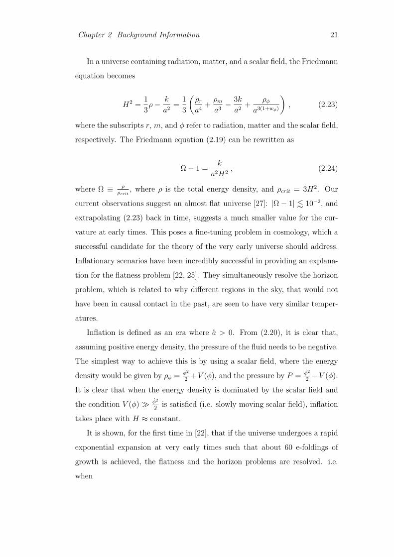
Chapter 2 Background Information 21
In a universe containing radiation, matter, and a scalar field, the Friedmann
equation becomes
H2 =1
3ρ− k
a2=
1
3
(ρr
a4+
ρm
a3− 3k
a2+
ρφ
a3(1+wφ)
), (2.23)
where the subscripts r, m, and φ refer to radiation, matter and the scalar field,
respectively. The Friedmann equation (2.19) can be rewritten as
Ω− 1 =k
a2H2, (2.24)
where Ω ≡ ρρcrit
, where ρ is the total energy density, and ρcrit = 3H2. Our
current observations suggest an almost flat universe [27]: |Ω− 1| . 10−2, and
extrapolating (2.23) back in time, suggests a much smaller value for the cur-
vature at early times. This poses a fine-tuning problem in cosmology, which a
successful candidate for the theory of the very early universe should address.
Inflationary scenarios have been incredibly successful in providing an explana-
tion for the flatness problem [22, 25]. They simultaneously resolve the horizon
problem, which is related to why different regions in the sky, that would not
have been in causal contact in the past, are seen to have very similar temper-
atures.
Inflation is defined as an era where a > 0. From (2.20), it is clear that,
assuming positive energy density, the pressure of the fluid needs to be negative.
The simplest way to achieve this is by using a scalar field, where the energy
density would be given by ρφ = φ2
2+V (φ), and the pressure by P = φ2
2−V (φ).
It is clear that when the energy density is dominated by the scalar field and
the condition V (φ) À φ2
2is satisfied (i.e. slowly moving scalar field), inflation
takes place with H ≈ constant.
It is shown, for the first time in [22], that if the universe undergoes a rapid
exponential expansion at very early times such that about 60 e-foldings of
growth is achieved, the flatness and the horizon problems are resolved. i.e.
when

Chapter 2 Background Information 22
ln
(ae
ai
)≈ 60 , (2.25)
where the subscripts e and i denote the end and the start of the inflationary era,
respectively. A more physically motivated definition for a general inflationary
scenario to solve the horizon problem can be given in terms of the size of the
comoving Hubble length. This is because the general inflationary condition
a > 0, is equivalent to the decrease in the rate of change of the Hubble radius,
i.e.d( 1
aH)
dt< 0. And, also, as originally argued in [22] and pointed out by
others more recently [86], it is the sharp reduction of 1aH
during inflation that
resolves the horizon problem. A more general and more physical definition for
the condition to solve this cosmological problem can, therefore, be written in
terms of the comoving Hubble length:
ln
(aeHe
aiHi
)= ln
(ae
ai
)≈ 60 . (2.26)
It is then clear that for the particular case of the standard inflationary scenario,
since the Hubble parameter is almost a constant, Eq. (2.26) reduces to the more
familiar form of Eq. (2.25). We will keep this in mind and return to this point
in the next chapter, where we will carry out an explicit investigation of how
LQC is capable of resolving the horizon problem.
By far, the most powerful result of inflation is its ability to account for the
density perturbation patterns observed on the Cosmic Microwave Background
(CMB) [17] and the accuracy with which this is done, together with the ex-
planation it offers for the origin of the large scale structure from quantum
perturbations.
During inflation, when the slow-roll condition is satisfied, from (2.23), it is
clear that in an expanding universe, the scalar field dominates the evolution of
the universe as the scale factor increases. It is also clear that during this rapid
expansion the contribution from the curvature is exponentially suppressed by
the scalar field resulting, effectively, in an exponentially flat universe.
The ekpyrotic model offers an alternative explanation to inflation with

Chapter 2 Background Information 23
many similar outcomes. Instead of a very flat positive potential for the slow-
roll process, imagine a very steep negative one, and instead of the universe
expanding, consider a contracting scenario. The equation of state then is
given by
wφ =φ2
2− V (φ)
φ2
2+ V (φ)
, (2.27)
where V (φ) is negative and steep in the ekpyrotic model, and since the field
is falling down fast due to the slope of the potential, wφ À 1. From (2.23),
it is clear that in a collapsing universe, once again, the scalar field becomes
dominant at late times (as a → 0), and in the process of contraction, for large
values of wφ, the curvature contribution is soon overtaken by the scalar field,
resulting in an effectively flat universe.
In order to realise such a physical scenario in the context of ekpyrotic
collapse, one first needs to obtain the background cosmology. For a universe
filled with a scalar field, imposing the solution to the Friedmann equation and
the continuity equation
H2 =1
3
(φ2
2+ V (φ)
), φ + 3Hφ + V,φ = 0 , (2.28)
to be a late time attractor, one finds the scaling background [101]
a = (−t)q , φ =√
2q ln(−t) , V (φ) = −V0e−σφ , (2.29)
where t is the cosmic time increasing from −∞ to 0−, V0 = q(1 − 3q), and
σ =√
2q. To find this cosmology, one may find it convenient to employ the
useful relation H = − φ2
2. For a contracting universe, q > 0, and a steep
potential implies q → 0+. The equation of state in this limit is given by
w =2
3q− 1 À 1 . (2.30)
Note that the contraction process is very slow, and the scalar field on this

Chapter 2 Background Information 24
steep potential can be thought of as a stiff fluid. Studying the quantum fluc-
tuations on this background can produce a near scale-invariant spectrum of
density perturbations in accordance with current observations [87]. The ekpy-
rotic model also predicts a large blue tilt for the gravitational waves produced
during this era, in great contrast to the small red tilt of tensor perturbations
obtained during inflation [88]. Consequently, the amplitude of these fluctua-
tions is suppressed by many orders of magnitude at large scales, compared to
the levels predicted by inflation. It has been claimed that this is the decisive
test, and if gravitational waves are observed on the CMB at levels of the order
predicted by inflation, the ekpyrotic model would be ruled out [88, 85].
2.3.2 The Shtanov-Sahni model
Another four dimensional effective cosmology model in the context of braneworlds,
which avoids the Big Bang singularity and is of interest in our phenomenolog-
ical studies in this work, is the simple Shtanov-Sahni model [78, 79, 94]. The
setup in this case is very similar to that of the R-S model with the exception of
the extra dimension being timelike. In this model, the brane tension is found
to be negative, and the Friedmann equation is modified such that
H2 =1
3ρ
(1− ρ
2|σ|)
, (2.31)
which at first instance has a very similar form to (2.18), but on closer inspec-
tion, quite different phenomenology is described here, and in fact, it is more
similar to the Holonomy corrections in LQC given by Eq. (2.16). Most impor-
tantly, an upper limit is implied on the possible level of the energy density,
close to which a bounce can occur, as discussed in subsection (2.2.2). Notice
that the additional ρ2 term in (2.31) modifies H from its form in standard
inflation
H = − φ2
2
(1− ρ
σ
). (2.32)
Here, too, soon after the universe starts expanding (i.e. σ < ρ ≤ 2σ), an

Chapter 2 Background Information 25
inflationary phase begins. Later in the expansion process, as the energy density
decreases (i.e. 0 < ρ ≤ σ), the condition for inflation becomes H2 > −H.
2.4 Fast-roll Inflation
In cosmologies where the energy density is dominated by a single scalar field,
both inflationary solutions and scaling solutions have been demonstrated to be
stable late time attractors (see [95, 96, 97] for early work in this field). Scaling
solutions are those in which the kinetic energy of the scalar field scales with its
potential energy when the energy density of the universe is dominated by the
scalar field. Standard slow-roll inflation has been studied extensively, and its
properties and predictions have been calculated to high precisions [98, 26, 99].
However, it is generally difficult to motivate such incredibly flat potentials
from fundamental theories. Steep potentials arise more commonly from un-
derlying physics (e.g. [80, 100, 18]). In order to see if such forms of scalar
potentials can be supported in the context of scaling solutions, as possible
alternatives to slow-roll inflation, one must first demonstrate that currently
observed phenomena could be incorporated within this framework. One of the
most important achievements of inflation has been its ability to explain the
near scale-invariance of density perturbations on the CMB. We now briefly
review the conditions under which this effect can be generated through a steep
potential, first discussed in [101].
Let us consider the simple case of a single scalar field, φ, on a potential,
V (φ), where the energy density ρ = φ2
2+ V , and the pressure P = φ2
2− V ,
lead to the equation of state w = P/ρ being a constant for scaling solutions.
In perturbation theory, the scalar perturbations of the metric, for a spatially
flat background in the Newtonian gauge, can be encoded by a single gauge
invariant variable, Φ, the Newtonian potential, such that [102]
ds2 = a2(τ)−(1 + 2Φ (τ, x)) dτ 2 + (1− 2Φ(τ, x)) dx2 , (2.33)
where τ is the conformal time related to proper time, t, by dt = a dτ .

Chapter 2 Background Information 26
By perturbing the scalar field φ → φ + δφ obeying the equation of motion
φ′′ + 2Hφ′ −∇2φ + a2V,φ = 0 , (2.34)
the differential equation for the perturbations in Fourier space becomes
(δφ)′′ + 2H(δφ)′ + (k2 + a2V,φφ)(δφ) = 0 , (2.35)
where a prime denotes differentiation with respect to τ , and H ≡ a′a.
Assuming a cosmological background, where the scale factor behaves as
a = (−τ)1
ε−1 , for a scaling solution to the standard Friedmann equations, the
equation of state is related to the slope of the potential by
ε ≡ 3
2(1 + w) =
1
2
(V,φ
V
)2
. (2.36)
We note here, that ε has the usual form of the slow-roll parameter. Upon
solving for δφ in (2.35), once normalisation has been done on small scales,
where quantum fluctuations are most important, in such a way that no particle
production takes place as modes evolve, the condition for near scale-invariance
translates to [101]
ε
(ε− 1)2¿ 1 . (2.37)
Notice that this condition is satisfied in two different limits of ε. First, when
ε → 0, which corresponds to w ≈ −1 (i.e. standard inflationary scenario), and
second, when ε →∞, corresponding to w À 1, which implies steep potentials.
We will refer to inflation arising from these potentials as ‘fast-roll’ inflation in
the remainder of this work.
Explicit calculations in [101] have shown that steep potentials in ekpyrotic
models generate a near scale-invariant spectrum of scalar perturbations. The
difficulty arises in quantifying any small deviation from exact scale-invariance.
In such models, since the field is evolving rapidly down the potential, it is not
appropriate to use the slow-roll parameters in an expansion, as ε will clearly

Chapter 2 Background Information 27
have a very large value. It is convenient, therefore, to introduce a ‘fast-roll’
parameter, instead, defined as
ε ≡ 1
2ε=
(V
V,φ
)2
, (2.38)
which will take small values in fast-roll inflation. By assuming a nearly con-
stant ε, one obtains
d ln ε
dN= −2
(V,φ
V
)(φ′
aH
)η , (2.39)
where N = ln a, and η is small and is defined by
η ≡ 1− V V,φφ
V 2,φ
. (2.40)
If one takes this parameter to be a constant (i.e. d ln ηdN
= 0), one could
then use the parameters ε and η to express the amount of deviation from exact
scale-invariance in scalar field fluctuations. We will use this method in the
context of LQC in the next chapter and the details of the calculation, which
have been omitted here, will be clearly explained.
2.5 Stability Analysis
Throughout this work stability analysis is carried out on many dynamical sys-
tems. A brief note is included here to cover the basic approach taken and to
outline the methods of phase plane analysis. (This is a well-studied concept
in the context of dynamical systems and chaos theory. See [103] for a sum-
mary and various applications of this method). Here, we demonstrate this by
taking a two-dimensional autonomous dynamical system of equations, where
the ordinary differential equations (ODEs) do not depend on the independent
variable, which is usually understood to be a dynamical parameter such as
time. It is then easy to generalise this approach to higher dimensional and
more complicated scenarios.
Let us consider the following equations
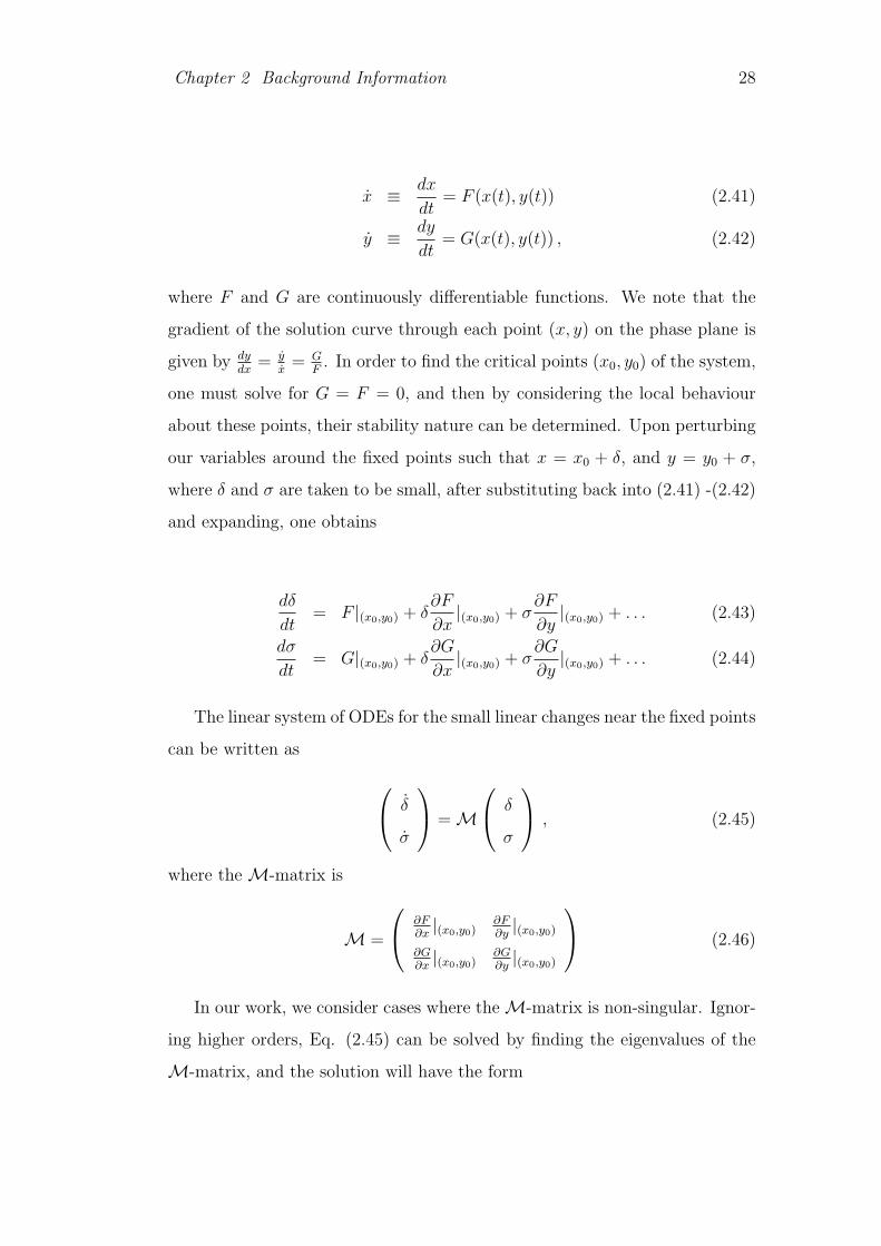
Chapter 2 Background Information 28
x ≡ dx
dt= F (x(t), y(t)) (2.41)
y ≡ dy
dt= G(x(t), y(t)) , (2.42)
where F and G are continuously differentiable functions. We note that the
gradient of the solution curve through each point (x, y) on the phase plane is
given by dydx
= yx
= GF. In order to find the critical points (x0, y0) of the system,
one must solve for G = F = 0, and then by considering the local behaviour
about these points, their stability nature can be determined. Upon perturbing
our variables around the fixed points such that x = x0 + δ, and y = y0 + σ,
where δ and σ are taken to be small, after substituting back into (2.41) -(2.42)
and expanding, one obtains
dδ
dt= F |(x0,y0) + δ
∂F
∂x|(x0,y0) + σ
∂F
∂y|(x0,y0) + . . . (2.43)
dσ
dt= G|(x0,y0) + δ
∂G
∂x|(x0,y0) + σ
∂G
∂y|(x0,y0) + . . . (2.44)
The linear system of ODEs for the small linear changes near the fixed points
can be written as
δ
σ
= M
δ
σ
, (2.45)
where the M-matrix is
M =
∂F∂x|(x0,y0)
∂F∂y|(x0,y0)
∂G∂x|(x0,y0)
∂G∂y|(x0,y0)
(2.46)
In our work, we consider cases where the M-matrix is non-singular. Ignor-
ing higher orders, Eq. (2.45) can be solved by finding the eigenvalues of the
M-matrix, and the solution will have the form
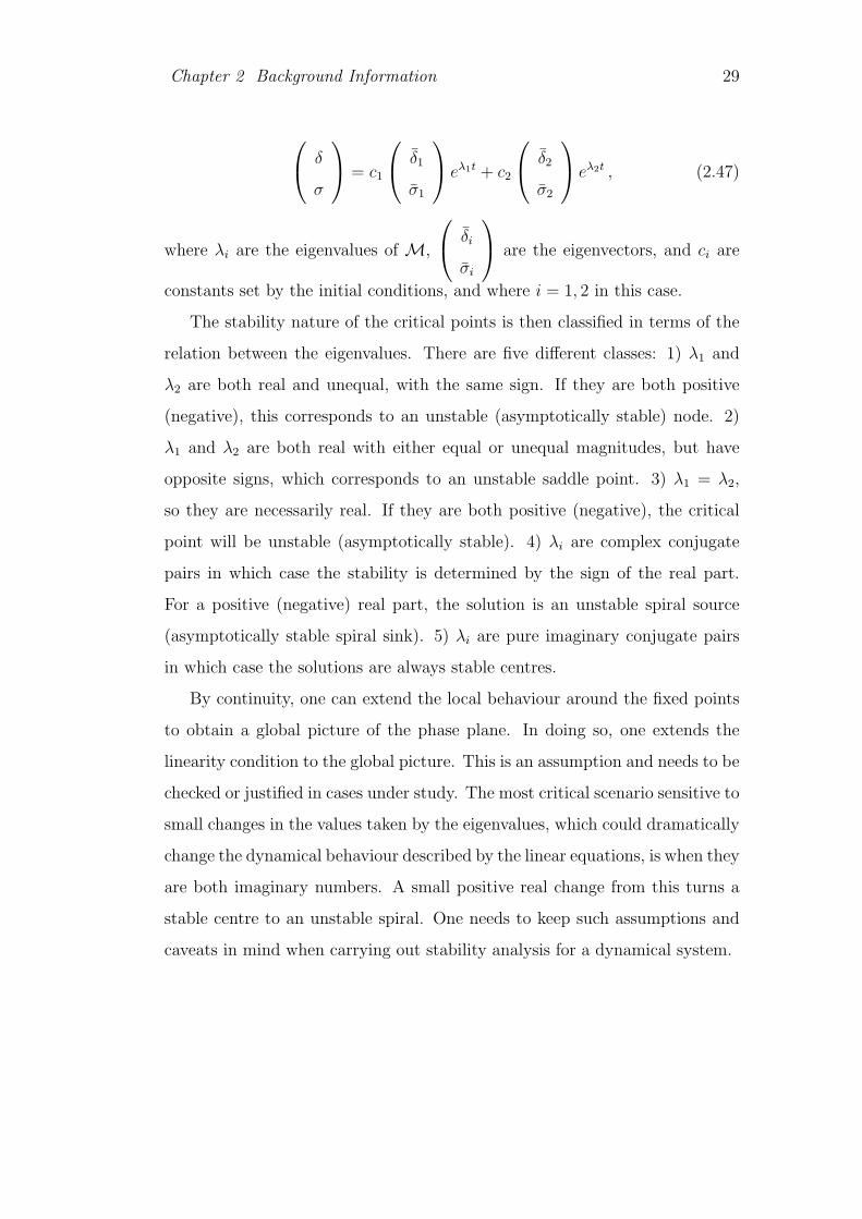
Chapter 2 Background Information 29
δ
σ
= c1
δ1
σ1
eλ1t + c2
δ2
σ2
eλ2t , (2.47)
where λi are the eigenvalues of M,
δi
σi
are the eigenvectors, and ci are
constants set by the initial conditions, and where i = 1, 2 in this case.
The stability nature of the critical points is then classified in terms of the
relation between the eigenvalues. There are five different classes: 1) λ1 and
λ2 are both real and unequal, with the same sign. If they are both positive
(negative), this corresponds to an unstable (asymptotically stable) node. 2)
λ1 and λ2 are both real with either equal or unequal magnitudes, but have
opposite signs, which corresponds to an unstable saddle point. 3) λ1 = λ2,
so they are necessarily real. If they are both positive (negative), the critical
point will be unstable (asymptotically stable). 4) λi are complex conjugate
pairs in which case the stability is determined by the sign of the real part.
For a positive (negative) real part, the solution is an unstable spiral source
(asymptotically stable spiral sink). 5) λi are pure imaginary conjugate pairs
in which case the solutions are always stable centres.
By continuity, one can extend the local behaviour around the fixed points
to obtain a global picture of the phase plane. In doing so, one extends the
linearity condition to the global picture. This is an assumption and needs to be
checked or justified in cases under study. The most critical scenario sensitive to
small changes in the values taken by the eigenvalues, which could dramatically
change the dynamical behaviour described by the linear equations, is when they
are both imaginary numbers. A small positive real change from this turns a
stable centre to an unstable spiral. One needs to keep such assumptions and
caveats in mind when carrying out stability analysis for a dynamical system.
Chapter 3
Super-inflation in LQC
3.1 Introduction
Given the importance of inflation and the need to explore all possibilities of
accommodating it in alternative theories of quantum gravity, in this chapter
we turn our attention to inflation in the context of Loop Quantum Gravity
(LQG) [14].
While the consequences of the quantum evolution in the semi-classical
regime of LQC are fascinating, it is difficult to connect it to existing the-
ories of the early universe which tend to be based on classical background
dynamics, and in particular to inflation. While the two sets of modifications
discussed in the previous chapter have rather different origins, it appears that
the qualitative effects of both the inverse volume effects and the ρ2 term are
rather similar. In particular, they both give rise to a period of super-inflation
during which the Hubble factor rapidly increases, rather than remaining nearly
constant as is the case during standard slow-roll inflation. Given that such a
super-accelerating phase appears to be a robust prediction of LQC, it is impor-
tant to study both the background dynamics, and particularly the cosmological
perturbations, which such a phase gives rise to. Considering a universe sourced
by a scalar field, a number of important results have already been obtained.
A scaling solution for the effective equations which arise from the inverse scale
factor modifications has been derived [63], and a number of attempts made
30

Chapter 3 Super-inflation in LQC 31
at studying perturbations in the super-inflationary regime [109, 100]. Simi-
larly the scaling solution for the ρ2 effective equation has also been derived
[110, 111].
It is also interesting to note the close connections between the super-
inflationary phases in LQC and the evolution of a universe sourced by a phan-
tom field, and with the ekpyrotic evolution of a collapsing universe [80, 81, 87,
83]. In all these cases the magnitude of the Hubble rate grows with time. More-
over, the scale factor duality discussed in [112] maps the ekpyrotic collapse onto
the super-inflationary scaling solution for the inverse volume modified equa-
tions. On the other hand, another duality maps the ekpyrotic collapse phase
onto the dynamics of a universe sourced by a phantom field [112]. These three
regimes are therefore all related to one another at the background cosmology
level. Furthermore, given that the ekpyrotic collapse is thought to offer a
method for the generation of scale-invariant perturbations [101] (as is the dual
super-inflationary phase sourced by a phantom field [113]), it is reasonable to
expect that a similar mechanism may operate in the super-inflationary phases
of LQC. Indeed such a mechanism has been discussed previously [100], though
its relation to ekpyrotic and phantom models was not emphasised.
In this study we aim to explore further the phenomenology of super-inflation
in LQC. One complication, however, is that the relative status of the two sets
of modifications discussed is at present unclear. We therefore take a pragmatic
approach and study the dynamics when each of the modifications is considered
in turn, but not including both sets of modifications simultaneously. In this
chapter, we focus our attention on perturbations in the scalar field as a first
approximation. This approach allows us to establish a framework for dealing
with metric perturbations in LQC. We will complete this study by turning our
attention to metric perturbations in the next chapter.
This chapter is organised as follows. In section 3.2, we introduce the cos-
mological evolution equations which arise in LQC including the inverse volume
corrections. Solutions are obtained including those showing scaling behaviour,

Chapter 3 Super-inflation in LQC 32
and the primordial spectrum of scalar perturbations is calculated for each so-
lution in terms of ‘fast-roll’ parameters. The stability of these solutions is
then discussed. In section 3.3, we analyse the dynamics when the modification
is induced by a ρ2 correction to the Friedmann equation. Concentrating on
the evolution just after the bounce, we demonstrate the existence of the super-
inflationary solution, obtain the scaling dynamics of the system, the primordial
spectrum of scalar perturbations as well as the stability of the background so-
lutions. Section 3.4 discusses the way in which super-inflation in LQC can
solve the horizon problem with a small number of e-foldings.
3.2 Effective field equations with LQC inverse
volume corrections
The first set of modified equations which we consider are those which incorpo-
rate the two functions, Dj,l(a) and Sj(a), defined in section 2.2.2, into the dy-
namics. These functions arise because of the presence of powers of the inverse
scale factor in the Hamiltonian constraint for an isotropic and homogeneous
universe.
The modified Friedmann equation is given by
H2 ≡(
a
a
)2
=κ2
3S
(φ2
2D+ V (φ)
), (3.1)
where κ2 = 8πG. In what follows we choose units in which κ = 1. Comparing
this equation with (2.15), we note that we have omitted the intrinsic curvature
contribution as we assume this to be a reasonable assumption. The equation
of motion for the scalar field takes the form [100]
φ + 3H
(1− 1
3
d ln D
d ln a
)φ−D∇2φ + DV,φ = 0 , (3.2)
where a subscript φ means differentiation with respect to the field. Comparing
this equation to Eq. (2.12), we see that the gradient term has been included

Chapter 3 Super-inflation in LQC 33
in order for us to be able to do a perturbation analysis. Strictly speaking,
this term violates the homogeneity assumtion, but we assume its effect on the
background cosmology can be safely neglected. These equations can also be
combined to give the Raychaudhuri equation
H = −S φ2
2D
[1− 1
6
d ln D
d ln a+
1
6
d ln S
d ln a
]+
S V
6
d ln S
d ln a. (3.3)
3.2.1 Scaling dynamics
We will be interested in the regime a ¿ a?, where the function Dj,l(a) may
be approximated by a power law of the form D(a) = D?an, where D? and n
are constants defined in the previous chapter with n taking values in the range
6 < n < ∞. Likewise, the function S(a) may be similarly approximated by
S(a) = S?ar, where S? and r are also constants introduced in the last chapter,
with r in the range 3 < r < ∞. For a À a? (i.e. in the classical limit),
S? ≈ D? ≈ 1 and r = n = 0. Inserting this form for the functions S and
D into Eq. (3.3), we can clearly see that for an expanding universe, and with
n > 6 + r, which occurs for all l, H is necessarily positive (assuming that the
potential is either positive or the term involving SV can be neglected). Hence
super-inflation is occurring. We will confine ourselves to these situations in
what follows.
To study this regime further, it proves convenient to introduce the variables
x ≡ φ√2Dρ
, y ≡√|V |√ρ
. (3.4)
where ρ ≡ φ2
2D+ V (φ). Using these definitions, the Friedmann equation (3.1)
and the equation of motion for the scalar field (3.2) can be written, for an
Chapter 3 Super-inflation in LQC 34
expanding universe, in terms of a system of first order differential equations as
x,N = −3αx±√
3
2λy2 + 3αx3 , (3.5)
y,N = −√
3
2λxy + 3αx2y , (3.6)
λ,N = −√
6λ2(Γ− 1)x +1
2(n− r)λ , (3.7)
where
λ ≡ −√
D
S
V,φ
V, Γ ≡ V V,φφ
V 2,φ
, (3.8)
with α = 1 − n/6 < 0 and N = ln a. These variables are subject to the
constraint equation
x2 ± y2 = 1. (3.9)
The plus and minus signs correspond to positive and negative potentials, re-
spectively. Using the constraint equation to substitute for y in Eq. (3.5)
renders Eq. (3.6) redundant.
The resulting system defined by Eq. (3.5) together with the constraint
equation and (3.7) has three fixed points for λ 6= 0. Two of them represent
kinetic energy dominated solutions, valid for all values of λ:
x = −1 , y = 0 , Γ = 1−√
6
12λ(n− r) , (3.10)
x = +1 , y = 0 , Γ = 1 +
√6
12λ(n− r) , (3.11)
and the third point is a scaling solution for which the kinetic and potential
energies evolve in a constant ratio to one another:
x =λ√6 α
, y =
ñ
(1− λ2
6α2
), (3.12)
Γ = 1 +α
2λ2(n− r) . (3.13)
The scaling solution is therefore well defined for λ2 < 6α2 for positive
potentials and for λ2 > 6α2 for negative potentials. In the remainder of this

Chapter 3 Super-inflation in LQC 35
analysis, we will focus mainly on the scaling solution for negative potentials as
this is the case that, as we shall see, leads to a scale invariant power spectrum
of the perturbed field.
Considering the fixed point for the scaling solution (3.12), one can write
φ√2Dρ
=
√S
D
φ,N√6
=λ√6α
, (3.14)
which upon integration gives
φ =2λ
(n− r)α
√D
S, (3.15)
where we have set the integration constant to zero without loss of generality.
Then inserting this relation into the definition of λ in (3.8) gives
V = V0 φβ , (3.16)
where β = −2λ2
(n−r)α> 0, and V0 is a constant.
Considering now the fixed point for y we have
V
ρ=
V S
3H2= 1− λ2
6α2. (3.17)
Obtaining an expression for φ in terms of a, from (3.15) in the semi-classical
regime, and substituting this into the form of the potential (3.16), and using
(3.17), the Hubble parameter can be found from which, by integration, the
behaviour of the scale factor can be determined as a function of time. This is
calculated to be a power law function, and in terms of the conformal time, τ ,
where dt = adτ , we find
a(τ) = (−τ)p , (3.18)
where for an expanding universe τ is negative and increasing towards zero, and
p =2α
2ε− (2 + r)α, (3.19)
Chapter 3 Super-inflation in LQC 36
where, for direct comparison with the previous chapter and Eq. (2.36), we have
introduced the slow-roll parameter ε ≡ λ2/2, and from (3.12), λ = −√2ε for
φ > 0. Using this form of a we find that H = paτ
, and it is straightforward to
show that
φ′(τ) = − 2√
2ε
2ε− (2 + r)α
√D
S
1
τ, (3.20)
V (τ) =4(3α2 − ε)
(2ε− (2 + r)α)2
1
S(aτ)2, (3.21)
where a prime means differentiation with respect to conformal time, τ . Equa-
tions (3.18) - (3.21) form the basis of our analysis.
3.2.2 Power spectrum of the perturbed field
For a universe which evolves according to the scaling solution, the primordial
spectrum of scalar perturbations produced by this super-inflationary phase
was previously calculated in Ref. [100]. It was found that the spectrum tends
to exact scale invariance for β À 1 (i.e. ε À 1), without any fine tuning of the
quantisation parameters of LQC. The purpose of this section is to review how
scale invariance arises for the scaling solution with β À 1, and to generalise
the analysis of [100] in order to allow for potentials which do not give rise to
exact scaling solutions.
In order to calculate the spectrum of perturbations, we now perturb the
scalar field equation (3.2) to linear order by using φ → φ + δφ, and V,(φ+δφ) =
V,φ + δφV,φφ + O(δφ2). The perturbation in the field δφ then satisfies the
equation
δφ′′ =[−2
a′
a+
D,τ
D
]δφ′ + D
[∇2 − a2V,φφ
]δφ , (3.22)
which can be written in the form [100]
u′′ +(−D∇2 + m2
eff
)u = 0 , (3.23)
where u is defined as u ≡ aD−1/2δφ and the effective mass of the field u is
Chapter 3 Super-inflation in LQC 37
given by
m2eff = −(aD−1/2)′′
aD−1/2+ a2DV,φφ . (3.24)
This change of variable clearly does not change the physical outcome, but it
allows (3.22) to be written in such a way that the first order term is eliminated.
It is then convenient to compare (3.23) with a harmonic oscillator equation.
We pause here to note that the first term inside the brackets of Eq. (3.23) is
reminiscent of the form obtained in the context of dynamics of a fluid with
a varying speed of sound (see [114, 115, 116, 117] for examples). Here, the
function D(a) plays the role of the square root of the effective speed of sound,
Cs. As it has recently been shown [118], for the case of Cs ≈ tp, where p is
a constant, there are two conditions under which scale invariance of the field
fluctuations may be obtained. Namely, p → 0 and p → −2. In the case of
the modified LQC equation (3.23), p = np2(1+p)
. The first condition corresponds
to either the classical case of n → 0, or p → 0, which as we shall see later,
is the scenario we will be interested in. The second condition corresponds to
n → −41+pp
, which in the limit of p → 0 results in very large values for n.
Although this has not been ruled out in the theory, the largest value quoted in
numerical simulations of LQC is of the order of 12. Therefore, the assumption
that allows us to proceed from this point to calculating the power spectrum of
the field fluctuations is that D(a) is a very slowly varying function of time. We
will see later in the chapter that this assumption is justified in our arguments
since the scale factor will be demonstrated to be a slowly varying function of
time during the super-inflationary phase under study.
Eq. (3.23) can also be obtained by varying the perturbed part of the action
in inverse volume corrected LQC [100]
δS =1
2
∫dτd3x(u′2 −Dδij∂iu∂ju−m2
effu2) . (3.25)
In order to consider quantum fields, we start by canonical quantisation of

Chapter 3 Super-inflation in LQC 38
this action to find the conjugate momentum, πu:
πu =∂L∂u′
= u′ . (3.26)
In quantum theory, the variables u and πu become operators u and πu,
respectively, obeying the usual commutation relations
[u(τ,x), u(τ,y)] = [πu(τ,x), πu(τ,y)] = 0 , [u(τ,x), πu(τ,y)] = iδ(x− y) ,
(3.27)
and the field equation for u is given by Eq. (3.23) once the following transfor-
mation is made:
u → u , and u′′ → u′′ . (3.28)
Decomposing u in Fourier modes uk, we have
u(τ,x) =
∫d3k
(2π)3[uk(τ)ak eik.x + u∗k(τ) a†k e−ik.x] , (3.29)
where uk satisfies the equation of motion
u′′k +(Dk2 + m2
eff
)uk = 0 , (3.30)
in Fourier space. The creation and annihilation operators ak and a†k obey the
usual commutation relations
[ak1 , ak2 ] = [a†k1, a†k2
] = 0 , [ak1 , a†k2
] = δk1k2 . (3.31)
It is then straightforward, but tedious, to verify that the commutation
relations in (3.27) and (3.31) are equivalent as long as the Wronskian condition
below is satisfied
u∗kduk
dτ− uk
du∗kdτ
= −i . (3.32)
For this system a unique vacuum state |0〉 can be defined [102] such that
ak|0〉 = 0 , ∀k , (3.33)

Chapter 3 Super-inflation in LQC 39
where the annihilation operators, ak, are the coefficients of the positive fre-
quency modes in the expansion of u given by Eq. (3.29). Since we are in-
terested in investigating quantum fluctuations arising from the vacuum, we
will concentrate on the forward moving (i.e. positive frequency) waves once
solutions to (3.30) are found, and then set the negative frequency components
to zero. This will also eliminate the possibility of particle production in the
vacuum.
The power spectrum for the quantum field, u(τ,x), which can be expanded
in Fourier space as in (3.29), is defined by [102]
Pu ≡ k3
2π2|uk|2 . (3.34)
The general solution to Eq. (3.30) is found to be given in terms of the
Bessel funtions as
uk(τ) = c1
√−τ J|ν|(x) + c2
√−τ Y|ν|(x) , (3.35)
where
ν = −√
1− 4 m2eff τ 2
2 + np, x =
2
2 + np
k√
D
aH, (3.36)
and where c1, c2, and meffτ are constants. This solution can also be rewritten
using the Hankel functions so that
uk(τ) =c1 − ic2
2
√−τ H(1)|ν| (x) +
c1 + ic2
2
√−τ H(2)|ν| (x) , (3.37)
where H(1)|ν| (x) = J|ν|(x) + iY|ν|(x) ∝ eix and H
(2)|ν| (x) = J|ν|(x)− iY|ν|(x) ∝ e−ix
are Hankel functions of the first and second kind, respectively. By rewriting the
solution in terms of these functions, one is able to conveniently decompose it in
terms of two plane waves propagating in two opposite directions. As mentioned
above, we follow the usual convention of standard inflationary scenario and
select only the advanced part by setting c1 = ic2, and ignoring the retarded

Chapter 3 Super-inflation in LQC 40
wave. Eq. (3.37) is then reduced to
uk(τ) = c1
√−τ H(2)|ν| (x) . (3.38)
In order to find the constant c1, one imposes the Wronskian condition (3.32).
This mode normalisation should be done at very high frequencies (i.e. k√
DaH
→∞), where quantum fluctuations in the vacuum are most important. By im-
posing this condition the solution (3.38) becomes
uk(τ) =
√π
2(2 + np)
√−τ H(2)|ν| (x) . (3.39)
On large scales (i.e. x ∝ k√
DaH
→ 0), by using the appropriate limits of the
Bessel functions
J|ν|(x) → 1
Γ(ν + 1)
(x
2
)ν
, Y|ν|(x) → −Γ(ν)
π
(2
x
)ν
, (3.40)
the power spectrum defined in Eq. (3.34), yields
Pu ∝ k3−2|ν| (−τ)1−|ν|(np+2) . (3.41)
Scale invariance of the power spectrum is then attained when the spectral tilt
∆nu ≡ 3− 2|ν| is zero.
For a universe evolving according to the scaling solution Eq. (3.18), we
have
m2effτ 2 = −2 + (3− 2n)p +
1
2(6 + 2n− n2)p2 , (3.42)
where we have used Eqs. (3.20)-(3.21), and (3.24). We can see from Eqs. (3.36),
(3.41), and (3.42) that scale invariance occurs whenever p → 0, which, as we
referred to, does indeed imply that ε À 1 and consequently V < 0 from
Eq. (3.21). There is one other value of p for which scale invariance is attained,
p = −4/(n + 4); however, we will not consider it any further, as there will be
an explicit dependence on the value of n in this case, and this parameter is
not well bounded within the context of LQC.
Chapter 3 Super-inflation in LQC 41
We would now like to generalise the form of the potential we are dealing
with so that it no longer has to be of exactly the form which gives rise to the
scaling solution. For standard slow-roll inflation, where the kinetic energy is
small compared with the potential energy, it is possible to account for poten-
tials of a form more general than a scaling potential by introducing slow-roll
parameters. Such parameters parametrise the steepness of the potential, and
how this steepness evolves as the field moves along the potential. For a given
field potential they also allow the dynamics which follow from a more general
potential to be expanded locally about the dynamics which follow from a scal-
ing potential with the same local steepness. The power spectrum which follows
from the general potential can then also be written in terms of the slow-roll
parameters.
For the case at hand we would like to develop a similar expansion scheme.
However, for the regime which we are considering in which ε À 1, it is clear
that the kinetic energy is of approximately the same magnitude as the potential
energy, and therefore the slow-roll approximation is inadequate. Indeed in this
case the field is evolving rapidly along a steep negative potential, and we
refer to the evolution as the ‘fast-roll’ regime, which we briefly touched on
in the previous chapter. Our strategy will therefore be to determine other
suitable small parameters which characterise the steepness and curvature of
the potential, and which we will refer to as ‘fast-roll’ parameters. The derived
parameters we will arrive at are similar to those described in the last chapter,
where fast-roll parameters were required to parametrise general potentials in
the ekpyrotic scenario. This similarity is natural since, as we have already
mentioned in the introduction, the evolution of the super-inflationary scaling
solution in LQC is dual to the ekpyrotic collapse.
The first step in accommodating a more general class of potentials is to
allow ε to become time dependent. From its definition it then follows that
ε′ = −(2ε)3/2 η
√S
Dφ′ , (3.43)
Chapter 3 Super-inflation in LQC 42
where we have defined
η ≡ 1− V,φφV
V 2,φ
− 1
2
V
V,φ
(D,φ
D− S,φ
S
), (3.44)
which can also be written in terms of the background quantities as
η ≡ 1− V,φφV
V 2,φ
− 1
2(n− r)
V
V,φ
a′
a φ′. (3.45)
Likewise, we can calculate η′ in terms of a third parameter ξ2,
η′ = −√
2ε ξ2
√S
Dφ′ , (3.46)
where
ξ2 ≡[1 +
V,φφφV
V,φφV,φ
− 2V,φφV
V 2,φ
]V,φφV
V 2,φ
+
−1
2
[1 +
D,φφ V
D,φ V,φ
− D,φV
DV,φ
− V,φφV
V 2,φ
]D,φV
DV,φ
+
+1
2
[1 +
S,φφ V
S,φ V,φ
− S,φV
SV,φ
− V,φφV
V 2,φ
]S,φV
SV,φ
. (3.47)
In particular, for the scaling solution where ε is constant, one can verify that
η = ξ2 = 0 exactly. Since we are considering potentials which are close to
the form of a scaling potential, we expect that there will be solutions to the
equations of motion of a form very similar to that given by Eqs. (3.18), (3.19),
(3.20) and (3.21), when ε is slowly varying. Assuming that Eqs. (3.18), (3.19)
and (3.20) are indeed good approximations, from (3.43) and (3.46), we have
thatd ln ε
d ln a≈ 4
ε η
α,
d ln η
d ln a≈ 2
ε ξ2
η α. (3.48)
Imposing that ε and η are slowly varying, and since ε is large in the regime
which gives rise to scale invariance, requires η and ξ2 to be small, i.e. the
potential must be nearly power law in form which is in agreement with our
assumption. We refer to η and ξ as the second and third fast-roll parameters,
Chapter 3 Super-inflation in LQC 43
and for convenience introduce the first fast-roll parameter as ε = 1/2ε. In
terms of relative magnitude we find, from the form of the potential (3.16),
β = −4ε(n−r)α
and ε À 1, that η ∼ ε and ξ2 ∼ O(ε2). Using these relations it
is possible to verify, by substituting Eqs. (3.18) – (3.21) into the Friedmann
equation and the equation of motion, that these solutions are indeed valid up to
second order in fast-roll parameters for a general negative potential confirming
the consistency of our analysis.
Substituting Eq. (3.19) into (3.42) and then evaluating ν in (3.36) to first
order in the parameters ε and η, we obtain
∆nu ≈ 4ε[1− n
12
(1 +
n
6− r
)− r
2
]− 4η , (3.49)
where we have made use of ∆nu ≡ 3 − 2|ν| in Eq. (3.41). We note that
although we have used the solution to Eq. (3.30) which is valid only when
meffτ is constant, the solution will remain sufficiently accurate provided that
ε does not vary significantly as a given k mode crosses the horizon from the
small wavelength to the long wavelength regime. This is simply the condition
that η is small, which we have assumed already. The spectral tilt can therefore
be calculated at any given scale by inserting into Eq. (3.49) the values that ε
and η take as this scale crosses the horizon. In particular, to compare with
observations we need to consider the mode which corresponds to the largest
scales on the Cosmic Microwave Background (CMB).
Finally we also note that we could include time derivatives of the powers
n and r. The generalisation to do so is straightforward and, following the
calculation process that led to Eq. (3.49), yields a more complicated expression
for the spectral index
∆nu ≈ 4ε[1− n
12
(1 +
n
6− r
)− r
2
]− 4η (3.50)
+ε
9τ n′ [8− 3(n− 6)− 4(r + n)]
+ε
9τ r′ [−8− 4(n− 6)] .
Chapter 3 Super-inflation in LQC 44
An explicit time dependance has now entered the expression for the spectral
tilt, which complicates the interpretation of this result. It does, however, imply
that for n ∝ r ∝ ln τ , a small constant value for the tilt will be recovered. For
simplicity we ignore such time derivatives and assume them to be small in our
region of interest.
3.2.3 Stability of the fixed points
The analysis we have performed so far is intriguing. It appears that in the a ¿a∗ regime, the scaling solution which follows from a steep negative potential
can give rise to a scale-invariant power spectrum of scalar field perturbations,
and moreover we can generalise the analysis to potentials which deviate from
the scaling potential.
However, there is another element which is involved in building a convinc-
ing theory for the origin of scale-invariant perturbations. That is, it would be
highly desirable if the scaling solution was an attractor, so that initial condi-
tions not exactly on the solution would evolve towards it, and the solution’s
stability against small local perturbations would be assured.
To determine the stability of the scaling solution, we study the nature of
the fixed points of Eqs. (3.5) and (3.7). We do this by linearising the equations
about the fixed points and determining the corresponding eigenvalues (ω) in
each case, using the method outlined in the previous chapter. For the kinetic
energy dominated solutions, valid for an arbitrary λ, in Eqs. (3.10) and (3.11),
we find their respective eigenvalues of the M-matrix
M =
−3α−√6xλ + 9αx2 −
√32(x2 − 1)
−√6(Γ− 1)λ2 −2√
6x(Γ− 1)λ + 12(n− r)
(3.51)
to be
ω+ = 6α +√
6λ , ω− = −1
2(n− r) , (3.52)
ω+ = 6α−√
6λ , ω− = −1
2(n− r) . (3.53)

Chapter 3 Super-inflation in LQC 45
Since n > r and α < 0, the first fixed point is stable for λ < −√6α and the
second for λ >√
6α. Turning to the scaling solution, Eq. (3.12), we find
ω± = − 1
4α
(θ ±
√θ2 + 8 α (n− r)(λ2 − 6α2
), (3.54)
where θ = α (6−r)−λ2 < 0. The scaling solution is therefore stable whenever
λ2 > 6α2, which coincides with the region of existence of this solution. In
Fig. 3.1 we show the evolution of the ratio −φ2/2DV obtained by numerically
solving the equations of motion. We can see that it approaches the value
given by x2/y2 where x and y are given by Eqs. (3.12). Tyically the evolution
only reaches the attractor when a > a? which is far outside the region where
the appoximation D ≈ an is valid. We conclude that this solution must be
extremely fine tuned in order to deliver the dynamics and power spectrum as
described in the previous subsections.
0 0.5 1 1.51
2
3
4
5
6
7
8
lna/a∗
-φ2/(2
DV
)
V = V0φ2
Figure 3.1: The evolution of the ratio −φ2/2DV obtained by numericallysolving the equations of motion for three different initial conditions (solid line).They approach the scaling solution given by x2/y2 where x and y are given byEqs. (3.12) (dashed line). We used as parameters V0 = −10−20, φinit = 1, inPlanck units and n = 15, r = 3 and ainit = 0.9a?, in a flat universe.
In the second part of this chapter we will be dealing with a second possibil-
ity of obtaining a super-inflationary regime that also leads to a scale invariant
power spectrum with the advantage that the stability of the scaling solution

Chapter 3 Super-inflation in LQC 46
is no longer a dangerous issue.
3.3 Effective dynamics with quadratic correc-
tions
The second modification to classical dynamics which we adopt follows from
considering that holonomies are the basic variables for quantisation in LQC.
This modification gives rise to a Friedmann equation of the following form
[51, 71, 50, 34, 53, 54]:
H2 =1
3ρ
(1− ρ
2σ
), (3.55)
which is identical to Eq. (2.16) that we first introduced in section 2.2.2. Once
again we are assuming either a flat universe or that the curvature contribution
can be safely neglected. It is interesting that this form of the Friedmann
equation is identical to the form which arises in braneworld scenarios with
a single time-like extra dimension spacetime [79]. In the braneworld case σ
represents the brane tension while for the LQC case 2σ represents the critical
energy density arising from quantum geometry effects which leads to the scale
factor undergoing a bounce as ρ approaches it from below.
We are interested in high density regimes where ρ approaches the bound-
ing value of 2σ. In this case, the term within brackets tends to zero, and the
behaviour of the equations alters significantly compared with the classical be-
haviour. Indeed in this regime we have H > 0 and for an expanding universe
super-inflation takes place. We will again consider a scalar field dominated
universe, hence, ρ = φ2/2 + V (φ). We stress that we are studying inverse vol-
ume and quadratic corrections separately, hence we do not include the D and
S functions in the Friedmann equation and in the definition of energy density.
The scalar field equation of motion
φ + 3Hφ + V,φ = 0 , (3.56)
Chapter 3 Super-inflation in LQC 47
is unchanged from the classical form.
3.3.1 Scaling dynamics
It was shown in Ref. [110] (also see [111]) that the effective equations (3.55)-
(3.56) also allow a scaling solution in which the kinetic and potential energy
vary in proportion to one another. In this case the potential must be of the
form V = V0cosh(φ). However, the scaling solution which was found implies
an evolution for the scale factor, which is not of a power law kind, and it has
not been possible to obtain analytical solutions to the equations of motion
of the scalar fluctuations, or for the spectrum of perturbations. It is, thus,
quite difficult to make general comments on the scale-dependence of such a
spectrum. Instead of focusing on the scaling solution we, therefore, take a
different approach and ask whether there is a form of the scalar field potential
which does result in a power law evolution of the scale factor. We are interested
in the regime in which ρ ≈ 2σ, when super-inflation occurs, and where H ≈ 0.
Inserting the power-law ansatz,
a(t) = (−t)m , (3.57)
where m is a constant, into the time derivative of the Hubble rate,
H = − φ2
2
(1− ρ
σ
), (3.58)
we see that for ρ ≈ 2σ the kinetic energy of the field is φ2/2 ≈ −m/t2 which
upon integration gives
φ ≈ ±√−2m ln t , (3.59)
from which we clearly need m < 0. Using Eq. (3.55) and expanding in
6H2/σ ¿ 1, solving for ρ, we have that
ρ ≈ 2σ − 3H2 , (3.60)

Chapter 3 Super-inflation in LQC 48
and it follows from the definition of the energy density of the field and Eq. (3.59)
that
V ≈ 2σ − U0e−λφ , (3.61)
where U0 = 3m2−m > 0 and λ = 1/√−2m. It is evident that, in this regime,
scaling exists between V − 2σ and the kinetic energy φ2/2. We now look for a
more precise description of the dynamics.
The form of the potential (3.61) motivates us to define the new variables:
x ≡ φ√4σ − 2ρ
, y ≡√
U√2σ − ρ
, (3.62)
such that ρ . 2σ and V (φ) = 2σ − U(φ). In terms of a system of first order
differential equations, the equation of motion of the scalar field now reads,
x,N = −3x−√
3
2λ y2 − 3x3 (3.63)
y,N = −√
3
2λxy − 3x2y (3.64)
λ,N = −√
6 λ2(Γ− 1)x + 3x2
(2σ
ρ− 1
) √2σ
ρ, (3.65)
where λ and Γ are defined as
λ ≡ −U,φ
U
√2σ
ρ, Γ ≡ U U,φφ
U2,φ
. (3.66)
The variables x, and y are also related by the constraint condition
x2 − y2 = −1. (3.67)
Considering the regime discussed above where 2σ/ρ ≈ 1, we can see λ is
a constant (remember λ = 1/√−2m), and by integrating λ in (3.66), we see
that the U part of the scalar potential is given by
U = U0 e−λφ , (3.68)

Chapter 3 Super-inflation in LQC 49
as we were expecting from Eq. (3.61).
We consider the section of the phase space in which x < 0, y > 0, and λ > 0.
Taking λ to be constant, and substituting the constraint equation (3.67) into
Eq. (3.63), results in an autonomous system with three fixed points. Two of
them are non-physical solutions with
x = ±i , y = 0 , (3.69)
and the third is a scaling solution with
x = − λ√6
, y =
√1 +
λ2
6. (3.70)
The scaling solution is valid for all real values of λ.
As in the previous case, it is straightforward to show that as the universe
evolves according to this solution,
φ√4σ − 2ρ
=φ,NH√4σ − 2ρ
= −λ
6, (3.71)
which upon integration, in the region ρ ≈ 2σ, yields
φ ≈ −λ ln a . (3.72)
The potential in Eq. (3.68) then is given in terms of the scale factor by
U ≈ U0aλ2
, (3.73)
and since this is a scaling solution (i.e. φ2 ∝ U), the Hubble parameter is
found to be
H2 ∝ aλ2
, (3.74)
and it is then easy to show that the scale factor undergoes a power law evolution
a(τ) = (−τ)p , (3.75)

Chapter 3 Super-inflation in LQC 50
where τ is the confrmal time, and where
p = − 1
ε + 1, (3.76)
and ε is here defined as ε = (U,φ/U)2/2 ≈ λ2/2. This is of course what
we expect since we began by searching for such a solution using the ansatz
Eq. (3.57). The time derivative of the field and the potential yields,
φ′ =
√2ε
ε + 1
1
τ, (3.77)
V = 2σ − 3 + ε
(1 + ε)2
1
(aτ)2. (3.78)
We are now ready to compute the spectrum of the scalar field perturbations
produced by this power-law solution.
3.3.2 Power spectrum of the perturbed field
In this section we follow the same approach we took in the previous analysis
of the scalar field perturbations. Similarly to our analysis presented in the
previous section, in terms of conformal time, the perturbation equation for the
scalar field, φ, can be written as
δφ′′ = −2a′
aδφ′ +
(∇2 − a2V,φφ
)δφ , (3.79)
which in turn can be written in terms of u ≡ aδφ as
u′′ +(−∇2 + m2
eff
)u = 0 , (3.80)
and the effective mass of the field u is
m2eff =
(−a′′
a+ a2V,φφ
), (3.81)

Chapter 3 Super-inflation in LQC 51
and by substituting Eqs. (3.75) - (3.78) into Eq. (3.81), we find
m2effτ 2 = −2 + 3p + 3p2. (3.82)
The change of variable from δφ to u is not essential, but helps intuitive
understanding of the physics of the system by eliminating the first order term
in (3.79) and reducing it to what resembles a harmonic osscilator. Eq. (3.80)
can also be obtained by varying the perturbed part of the action in holonomy
corrected LQC
δS =1
2
∫dτd3x(u′2 − δij∂iu∂ju−m2
effu2) . (3.83)
Following the steps taken in the previous section to produce Eq.s (3.26)-
(3.29), yields Fourier modes uk, that satisfy
u′′k +(k2 + m2
eff
)uk = 0 , (3.84)
and the power spectrum is then defined by
Pu ≡ k3
2π2|uk|2 , (3.85)
and it is clear that the Wronskian condition given by (3.32) remains unchanged.
The general solution to Eq. (3.84) is found to be given in terms of the
Bessel funtions as
uk(τ) = c1
√−τ J|ν|(x) + c2
√−τ Y|ν|(x) , (3.86)
which can be rewritten using the Hankel functions so that
uk(τ) =c1 − ic2
2
√−τ H(1)|ν| (x) +
c1 + ic2
2
√−τ H(2)|ν| (x) , (3.87)

Chapter 3 Super-inflation in LQC 52
whenever meffτ is constant. The constant, ν, and the variable, x, are given by
ν = −√
1− 4 m2eff τ 2
2, x =
k
aH, (3.88)
where c1 and c2 are constants. H(1)|ν| (x) and H
(2)|ν| (x) are Hankel functions of the
first and second kind, respectively. Using these functions we can once again
conveniently decompose the solution in terms of two plane waves propagating
in two opposite directions. We follow our previous line of argument, and that
of the usual convention of standard inflationary scenario, and select only the
advanced part by setting c1 = ic2. This sets the retarded wave equal to zero,
which, as argued in the previous section, has the consequence of no particles
being produced in the vacuum. Eq. (3.87) is then reduced to
uk(τ) = c1
√−τ H(2)|ν| (x) . (3.89)
In order to find the constant c1, following our previous method, we impose
the Wronskian condition (3.32), and find
uk(τ) =
√π
4
√−τ H(2)|ν| (x) . (3.90)
On large scales (i.e. kaH→ 0), by using the appropriate limits of the Bessel
functions, as before, the power spectrum can be approximated by
Pu ∝ k3−2|ν| (−τ)1−2|ν| . (3.91)
Consequently, the spectral tilt is defined, as before, by ∆nu ≡ 3− 2|ν|. By
substituting (3.82) into (3.88), we see that we expect to have scale invariance
of field perturbations for p → 0. Once again, therefore, scale invariance occurs
when the field φ is rolling down a steep potential and the kinetic energy is not
negligible, but comparable to V − 2σ. Hence the evolution should again be
understood as a fast-roll regime.
Clearly, scale invariance is also obtained for p → −1 or ε ¿ 1 which

Chapter 3 Super-inflation in LQC 53
corresponds to the standard slow-roll regime that we are not concerned with
for the purposes of this work.
In order to extend this analysis to general potentials, as we did for the
previous system of modified equations we studied, we allow ε to depend on
conformal time such that
ε′ = −(2ε)3/2η φ′ , (3.92)
which defines the fast-roll parameter η,
η ≡ 1− U,φφU
U2,φ
. (3.93)
Similarly, η′ can be written in terms of the next order fast-roll parameter ξ2
as
η′ = −√
2ε ξ2 φ′ , (3.94)
with
ξ2 ≡(
1 +U,φφφU
U,φφU,φ
− 2U,φφU
U2,φ
)U,φφU
U2,φ
. (3.95)
For the exact scaling solution, it can be verified that both η and ξ2 van-
ish. As in the previous case, we can use Eqs. (3.75), (3.76) and (3.77) as
approximate solutions, and hence we have
d ln ε
d ln a≈ 4εη ,
d ln η
d ln a≈ 2
εξ2
η, (3.96)
where we have again defined a further fast-roll parameter by ε = 1/2ε. This
means that for a large and slowly varying ε the parameter η must be small,
and for a slowly varying η the parameter ξ2 must also be small. Hence, the U
part of the scalar potential must be close to exponential.
Using Eqs. (3.75) - (3.77) in the expression for the effective mass of u,
Eq. (3.81), where ε is now time dependent, and then using Eq. (3.88), we find
that ∆nu ≡ 3− 2|ν| is to first order
∆nu = −4(ε− η) . (3.97)

Chapter 3 Super-inflation in LQC 54
Again the assumption that meffτ is nearly constant as a given mode evolves
outside the cosmological horizon is valid. Hence the spectral tilt for a given k
mode can be calculated by inserting the values the fast-roll parameters took
as the mode crossed the horizon in Eq. (3.97). It is clear that the system
we have investigated here results in a scale-invariant spectrum of scalar field
perturbations for ε ¿ 1 and η ¿ 1.
3.3.3 Stability of the fixed points
Following our previous stability analysis, using the constraint Eq. (3.67) to
substitute for y in (3.63) and (3.65), and linearising the system, we find the
M-matrix
M =
−3−√6xλ− 9x2 −
√32(x2 + 1)
−√6(Γ− 1)λ2 + 6xµ −2√
6x(Γ− 1)λ + 3x2µ
, (3.98)
where µ =(
2σρ− 1
) √2σρ
. The eigenvalues, ω, are then given: for the unphys-
ical kinetic energy dominated solution, Eq. (3.69),
ω = 6± i√
6λ , (3.99)
and, hence, this solution is unstable. While for the scaling solution, Eq. (3.70)
ω = −1
2(6 + λ2) , (3.100)
and, hence, this point is a stable attractor for all values of λ. A numerical
analysis of this system shown in Fig. 3.2 supports our analytical results pre-
sented here. The figure shows the evolution of the ratio φ2/(2σ− V ) obtained
by numerically solving the equations of motion for three different initial con-
ditions. They approach the scaling solution given by 2x2/y2 where x and y
are given by Eqs. (3.70). When a À a? the quadratic corrections become
negligable and the numerical evolution diverges from this attractor.
In our calculation we have neglected metric perturbations, and instead, we

Chapter 3 Super-inflation in LQC 55
have only considered scalar perturbations and been able to find scale-invariance
through the scalar field perturbations.
0 2 4 6 80
0.05
0.1
0.15
0.2
0.25
lna/ainit
φ2/(2
σ−
V)
U = U0 exp(− φ)
Figure 3.2: The evolution of the ratio φ2/(2σ−V ) obtained by numerically solv-ing the equations of motion for three different initial conditions (solid lines).They approach the scaling solution given by 2x2/y2 where x and y are givenby Eqs. (3.70) (dashed line). We used as parameters U0 = 10−2, φinit = 1 andσ = 0.41 in Planck units, in a flat universe.
3.4 Number of e-folds
Before concluding, it is important to address the question of whether a suf-
ficient amount of super-inflation can occur in LQC to account for the largest
scale perturbations observed on the CMB. This in turn is equivalent to ask-
ing whether the super-inflationary phases can solve the cosmological horizon
problem.
It is clear that only a small number of e-folds of super-inflation can be
considered generic for either of the modified sets of evolution equations we
have studied [62]. This might be considered disappointing, since experience
from standard inflation suggests that approximately 60 e-folds of inflation are
required for consistency with observations. However, the inflationary periods
we have been studying are considerably different to standard inflation and this
has a dramatic effect.

Chapter 3 Super-inflation in LQC 56
Solving the horizon problem is essentially the requirement that aH grows
sufficiently during an early stage of the universe’s evolution. While in stan-
dard inflation this is accomplished by a changing rapidly as H remains nearly
constant, in our case the converse appears to be possible, that H increases
sufficiently as a remains nearly constant. The number of e-folds usually only
refers to the change in a, and so we only expect a small number of e-folds to be
necessary in a super-inflationary phase, provided that H changes sufficiently.
To confirm the expectation that our super-inflationary phases can indeed solve
the horizon problem, let us now quantify our qualitative arguments.
During super-inflation, perturbation modes exit the cosmological horizon,
and once super-inflation ends, modes start to re-enter. Let us consider a
perturbation mode with wavenumber k, such that k exited the cosmological
horizon N(k) e-folds before the end of the super-inflationary phase, and re-
entered sometime later. The mode re-entering the horizon today, k∗, must
satisfy k∗ = a0H0, where subscript 0 indicates quantities at the present epoch.
Comparing this with the generic k mode we have:
k
a0H0
=akHk
a0H0
=akHk
aendHend
aend
areh
areh
aeq
aeq
a0
Hend
H0
, (3.101)
where subscript ‘end’ labels quantities at the end of inflation, ‘reh’ at reheat-
ing, and ‘eq’ at matter radiation equality. For simplicity, assuming that the
universe behaves as if it is matter dominated between the end of inflation and
reheating, we have
k
a0H0
=akHk
aendHend
(ρend
ρreh
)−1/3 (ρreh
ρeq
)−1/4 (ρeq
ρ0
)−1/3Hend
H0
, (3.102)
which can also be written as
k
a0H0
=akHk
aendHend
(ρend
ρreh
)−1/12 (ρeq
ρ0
)−1/12 (ρend
ρ0
)−1/4Hend
H0
, (3.103)

Chapter 3 Super-inflation in LQC 57
which upon using H2 = 13ρ, becomes
k
a0H0
=akHk
aendHend
(ρend
ρreh
)−1/12 (aeq
a0
)−1/4 (Hend
MPl
)1/2 (MPl
H0
)1/2
. (3.104)
Then employing the known evolution of the universe from equality to the
present day (i.e a0
aeq= 1+ zeq ≈ 1000), together with the measured value of the
Hubble rate at the present epoch, H0, we find:
ln
[k
a0H0
]≈ 68 + ln
[akHk
aendHend
]− 1
2ln
[MPl
Hend
]− 1
3ln
[ρend
ρreh
]1/4
. (3.105)
The energy scale at the end of inflation must be determined by requiring that
the magnitude of the curvature perturbation accounts for the temperature
anisotropies in the CMB. Since we have only worked with the scalar field
perturbation this is so far undetermined in our model and we therefore take
Hend to be the highest possible scale, i.e. Hend = MPl. A lower scale would
lead to fewer required e-folds. Further considering k = k∗ and assuming instant
reheating, we find that
ln
(aendHend
ak∗Hk∗
)≈ 68 . (3.106)
In order to determine the number of e-folds of super-inflation required, we
now consider the cases in which the scale factor is undergoing pure power-law
behaviour, a ∝ (−τ)p. Using this together with Eq. (3.106), we find
ln
(τend
τk∗
)−1
≈ 68 , (3.107)
and in turn
N(k∗) = ln
(aend
ak∗
)= −68 p . (3.108)
Recalling that p must be small and negative for scale invariance, we see that
only a small number of e-folds are required. Although considering behaviour
which deviates from pure power law behaviour will alter Eq. (3.108), it is
clear that the conclusion of only a small number of e-folds being necessary will
remain valid. We will proceed in the next chapter to investigate the role of

Chapter 3 Super-inflation in LQC 58
tensor perturbations in LQC.
Chapter 4
The gravitational wave
background from super-inflation
in LQC
4.1 Introduction
A key result of the inflationary scenario of the very early universe [22, 25, 26]
is that it gives rise to a stochastic background of gravitational wave radiation
(tensor perturbations) [122]. Such a background is in principle observable
and could be used to distinguish between different models of inflation [123].
Alternative proposals such as the ekpyrotic/cyclic scenario [80, 81, 82, 83,
87, 84, 88, 85] or phantom super-inflation [113, 124] lead to very different
predictions for the spectral tilt of tensor perturbations when compared with the
simplest inflationary models [88], implying the gravitational wave background
could also be a powerful discriminator between competing theories. In this
chapter we will be concerned with the gravitational wave background produced
by super-inflationary scenarios within Loop Quantum Cosmology (LQC).
Following the analysis we carried out in the previous chapter, one point to
note here is the assumption of a purely isotropic universe. In the regime of
very small scale factor, the discrete structure of space is so strong that any
inhomogeneous configuration would be far from being isotropic. Therefore,
despite being able to write the effective perturbation equations for a purely
59
Chapter 4 The gravitational wave background from super-inflation in LQC 60
isotropic scenario in this regime, one should keep in mind that in reality care
needs to be taken regarding the cosmological interpretation of perturbations
and their evolution [48, 125].
In the previous chapter we did not consider the spectrum of tensor per-
turbations produced in the cosmologies we discussed. This is the question to
which we now turn. This question is particularly timely since the effect of the
two kinds of modifications on the evolution of tensor perturbations in LQC
has only recently been derived [69].
Similar calculations have already been carried out and reported in the lit-
erature for different types of cosmologies. In particular, gravitational wave
perturbations for ekpyrotic models of a collapsing universe [88], and for phan-
tom superinflaion scenarios [124] have been computed. Despite being based on
different physical concepts and behaviours, both cosmologies predict a strongly
blue tilted spectrum of tensor perturbations, and since these have not yet been
observed, it suggests that in both scenarios, the amplitude of these fluctua-
tions are suppressed on large scales by many orders of magnitude compared to
those predicted by standard inflation. This is not unexpected, as it has been
pointed out in Ref. [112] that a duality exists between the ekpyrotic collapse
and the dynamics of a universe sourced by a phantom field. Moreover, a scale
factor duality maps the ekpyrotic collapse onto the superinflationary scaling
solutions in LQC [63].
Given the connections found between LQC and the ekpyrotic and phantom
scenarios, one might expect that LQC also predicts a large blue tilted spectrum
for the tensor perturbations. However, as the connections are at the level of
the background equations and since LQC corrections also arise in the evolution
equations of tensor perturbations themselves, this expectation may not be
realised and a careful analysis is necessary to confirm it.
The structure of this chapter is as follows. In Section 4.2, we discuss the
inverse triad modifications. First we review the background dynamics which
give rise to a scale invariant spectrum of scalar field perturbations, and then we
consider the evolution of tensor perturbations in this setting calculating their
Chapter 4 The gravitational wave background from super-inflation in LQC 61
spectrum. We then repeat the exercise for holonomy corrections in section 4.3.
Finally we conclude in section 4.4.
4.2 Tensor dynamics with inverse triad cor-
rections
We first consider the cosmological equations which follow from including mod-
ifications associated with the inverse triad in the semi-classical regime of LQC.
Whilst recognising the careful attention this regime deserves, and acknowledg-
ing more work is required to clarify the validity of the dynamical equations
we use together with the assumption of isotropy, we hope to pave the way by
demonstrating a method of calculation which can easily be employed once new
light is shed on currently uncertain sections of the theory.
The unperturbed isotropic modified Friedmann equation is given by Eq. (2.15),
which in terms of the conformal time becomes
H2 ≡(
a′
a
)2
=κ2
3S
(φ′2
2D+ a2V (φ)
), (4.1)
where a dash represents differentiation with respect to conformal time, τ , and
we have assumed that any curvature contribution has become subdominant.
The scalar field equation of motion is similarly given by Eq. (2.12), which in
terms of τ becomes
φ′′ + 2H(
1− 1
2
d ln D
d ln a
)φ′ + a2DV,φ = 0 . (4.2)
In this chapter our interest is in the evolution of tensor perturbations about
this isotropic background. Tensor perturbations are defined as the transverse
and trace free part of the perturbed spatial metric, and represent gravitational
wave perturbations propagating on the unperturbed background spacetime.
They can be further decomposed into two polarisation modes represented by
× and +, and in LQC, with inverse triad modifications included, the equation
Chapter 4 The gravitational wave background from super-inflation in LQC 62
of motion for these modes has recently been derived to be [69]
h′′×,+ + 2H[1− 1
2
d ln S
d ln a
]h′×,+ − S2∇2h×,+ = 0 . (4.3)
h×,+ is a tensorial quantity, but from here on to avoid clutter we will drop
the × and + subscripts, and take h to represent the magnitude of one of the
polarisation modes, but always keep in mind that both modes are present.
4.2.1 The background power law solution and scale in-
variant scalar field dynamics
As we demonstrated previously, in section 3.2, in the regime a ¿ a?, there
exists a power law solution to the equations of motion (4.1)–(4.2) which is a
stable attractor to the dynamics. This solution exists for negative power law
potentials of the form V = V0 φβ (with V0 < 0) and gives rise to the dynamics
a(τ) = A(−τ)p , (4.4)
φ′(τ) = −√
p2 + (r + 2)p
α
√D
S
1
τ, (4.5)
V (τ) =
(3− 2 + (r + 2)p
2α
)1
S(aτ)2, (4.6)
where for an expanding universe τ is negative and increasing from −∞ towards
zero. A is an arbitrary normalisation constant, and α = 1− n/6 with β and p
being related through
β = −2
p
2 + (r + 2)p
n− r. (4.7)
Notice the equivalence between these equations and (3.20) - (3.21) derived in
the previous chapter, where we expanded about this solution in terms of fast-
roll parameters, in order to generalise the potentials which can be considered.
Here, for simplicity we will consider only this exact solution.
For −1 < p < 0 the solution given above represents a universe undergo-
ing super-inflationary evolution during which the Hubble rate increases. A
particularly interesting case then occurs as p tends to zero from below. This
Chapter 4 The gravitational wave background from super-inflation in LQC 63
represents a universe in which the scale factor is almost constant, but H in-
creases rapidly. Considering scalar field perturbations about the background
field, we showed in section 3.2 that the spectrum of scalar field perturbations
attains scale-invariance in this limit. Moreover, because H increases so rapidly,
the horizon problem is solved during this phase with only a small number of
e-folds required. This raises the intriguing possibility that these perturbations
could be responsible for the observed CMB anisotropies and hence for struc-
ture in the universe. If this were the case, no period of standard inflation in
which H remains nearly constant for roughly 60 or more e-folds of expansion
would be required (where number of e-folds is defined as N = ln(a/ai)). A
natural, and indeed important question is: ‘what is the spectrum of primordial
tensor perturbations which accompanies this scale invariant spectrum of scalar
field perturbations?’. This is the question to which we now turn.
4.2.2 The primordial spectrum of tensor perturbations
To calculate the spectrum of gravitational waves produced during super-inflation
we follow the standard procedure. Given that −a2h/2 is canonically conjugate
to h′/(2S) such that [69]
1
2Sh′(t, x),−a2
2h(t, y)
= δ3(x, y) , (4.8)
the system is quantised by promoting h and h′ to operators and the Poisson
brackets to commutators. We have
[h′, h
]= −4i
S
a2δ3(x, y) . (4.9)
h is then decomposed into Fourier modes
h =
∫d3k
(2π)3/2
[hk(τ)ake
ik·x + h∗k(τ)a†ke−ik·x
], (4.10)

Chapter 4 The gravitational wave background from super-inflation in LQC 64
where, considering Eq. (4.3), we see that each mode hk obeys the evolution
equation
h′′k + 2H(
1− 1
2
d ln S
d ln a
)h′k + S2k2hk = 0 , (4.11)
in Fourier space. The power spectrum for one polarisation state of tensorial
fluctuations is given by the standard expression
Ph =k3
2π2|hk|2 . (4.12)
In order to evaluate Eq. (4.12) we must solve Eq. (4.11). Considering the
power law solution for the regime a ¿ a? (given by Eq. (4.4)), and using the
form of S in this regime (S = S∗ar), we find that Eq. (4.11) becomes
h′′k + 2p
τ
(1− r
2
)h′k + k2S2
?A2r(−τ)2rphk = 0 , (4.13)
with the general solution
hk(τ) = c1S1/2
H1/2aJν(x) + c2
S1/2
H1/2aYν(x) , (4.14)
where Jν(x) and Yν(x) are Bessel functions of the first and the second kind,
respectively. c1 and c2 are constants, and the constant ν and the variable x
are given by
ν =1 + p(r − 2)
2(1 + pr), x =
−pSk
(1 + pr)H . (4.15)
Eq. (4.14) can also be rewritten in terms of the Hankel functions, so that
hk(τ) =c1 − ic2
2
S1/2
H1/2aH(1)
ν (x) +c1 + ic2
2
S1/2
H1/2aH(2)
ν (x) , (4.16)
where H(1)ν (x) = Jν(x) + iYν(x) and H
(2)ν (x) = Jν(x) − iYν(x) are the Hankel
functions (also known as the Bessel functions of the third kind). As mentioned
in the previous chapter, this decomposition of our solution allows it to be
written in terms of two plane waves moving in opposite directions. Once again,
we adopt the general convention of standard inflationary scenario and select

Chapter 4 The gravitational wave background from super-inflation in LQC 65
the forward moving wave. Neglecting the retarded wave, by setting c1 = c2,
reduces Eq. (4.16) to
hk(τ) = c1S1/2
H1/2aH(2)
ν (x) . (4.17)
Before going any further from this point, it is worth pausing to give a
brief outline of the analysis which should be followed to find the constant,
c1. We start from the perturbed densitised triad and the extrinsic curvature
perturbations in the classical regime, given by [69]
δE = −1
2ph , (4.18)
δK =1
2[h′ +Hh] , (4.19)
where p = a2 (not to be confused with p in Eq. (4.4)), and where, for simplicity,
we have dropped all indices. Using the knowledge that these quantities are
canonically conjugate to one another
δKx , δEy = δ(3)(x− y) , (4.20)
one obtains
1
2[h′ +Hh]x , −1
2a2hy = 1
2au′x , −1
2auy , (4.21)
where u ≡ ah. Once these parameters have been promoted to operators and
the Poisson brackets to commutation relations, we get
[−1
4u′x , uy] = iδ(3)(x− y) , (4.22)
and it is then clear that −14u′ is the conjugate momentum of u.
In Fourier space, by expanding u(τ,x)
u(τ,x) =
∫d3k
(2π)3/2[wk(τ)ake
ik.x + w∗k(τ)a†ke
−ikx] , (4.23)
and calculating the commutation relation of (4.22), upon using the usual com-
mutation relations for the creation and the annihilation operators, a† and a,
Chapter 4 The gravitational wave background from super-inflation in LQC 66
we find
[u′x , uy] = (u∗kuk,τ − uku∗k,τ )δ
(3)(x− y) . (4.24)
Comparing this result to Eq. (4.22), we arrive at the Wronskian condition
u∗kuk,τ − uku∗k,τ = −4i . (4.25)
Notice that although this is the usual form in which this condition is gen-
erally written, in our analysis, there is no need (other than for convenience) to
introduce the parameter u in the formulism. However, it is not always possible
to introduce an analogous parameter which simplifies the formulism, so one
may need to go back a step and expand the tensor perturbations operator, h,
directly (as in Eq. (4.10)). The effect of this on the Wronskian condition is
easily seen to be
h∗khk,τ − hkh∗k,τ = − 4
a2i , (4.26)
and by following the method above, it can be shown that the conjugate mo-
mentum of h is given by −a2
4h′.
In the case of the inverse triad corrections, Eq. (4.19) is found to be modified
such that [69]
δK =1
2[h′
S+Hh] . (4.27)
Once again, by employing Eq.s (4.18) and (4.20), the conjugate momentum
of h is found to be − a2
4Sh′, and the Wronskian condition becomes
h∗khk,τ − hkh∗k,τ = −4S
a2i . (4.28)
This condition is equivalent to requiring no particle production in the vac-
uum for it to be well defined, and so must be satisfied at very early times when
the quantum fluctuations are most likely to create particles inside the vacuum.
This corresponds to the limit of very high frequencies (low wavelengths), i.e.

Chapter 4 The gravitational wave background from super-inflation in LQC 67
Sk/H →∞. In this regime, Eq. (4.17) can be approximated by
hk(τ) ≈ c1S1/2
H1/2a
√−2(1 + pr)H
pπSke−i pSk
(1+pr)H . (4.29)
By substituting this result back into Eq. (4.28), and finding the constant
c1, the exact solution for the tensor perturbations is found to be
hk(τ) =S1/2
H1/2a
√ −p π
1 + rpH(2)
ν (x) . (4.30)
This solution has the expected behaviour that each k mode begins in an
oscillatory state where normalisation occurs, and evolves into a non-oscillatory
state once each given k mode crosses a suitably defined horizon. From the form
of (4.30) and (4.15), it is clear that for tensor modes horizon crossing occurs
when k ≈ −aH/pS. A given mode can only be considered to become a classical
perturbation once it crosses this horizon.
Taking the solution (4.30) and employing (4.12) we find that
Ph =22(ν−1)
π2
Γ(ν)2
Γ(3/2)2
(k0
ke
)3−2ν (k
k0
)3−2ν
H2e , (4.31)
where we have evaluated (4.30) in the limit where the modes are outside the
defined horizon (i.e. x → 0), by using the appropriate limits of the Bessel
functions given by Eq. (3.40), and it can be seen that we have also accounted
for both polarisation states. The mode k0 corresponds to the largest scales on
the CMB and ke is defined as the last mode to cross the horizon at the end of
super-inflation (ke = He/Se ≈ He).
A couple of observations are in order. The first is that in the limit of
interest, p → 0, the spectrum is blue tilted with a tensor spectral index given
by
nt = 2 +2p
1 + rp≈ 2 , (4.32)
where nt is defined, as usual, by Ph ∝ knt . This implies that on large scales
the spectrum is hugely suppressed. The second important point is that the

Chapter 4 The gravitational wave background from super-inflation in LQC 68
magnitude of the spectrum is fixed by the Hubble rate at the end of infla-
tion. This also fixes the magnitude of scalar perturbations and ultimately
has to be normalised such that the scalar perturbations have the correct mag-
nitude to account for the CMB anisotropies. In the scenario at hand such
a normalisation is difficult to determine since the scalar field perturbations
(which are close to scale invariant) must be related to curvature perturbations
(as discussed in the previous chapter and in [18]), and this step cannot be
performed at present. Nevertheless in the following section we will make the
reasonable assumption that He corresponds to the GUT scale (1014GeV ), in
order to calculate the present-day spectrum of gravitational waves produced
by this super-inflationary scenario. By assuming a radiation dominated uni-
verse between now and the end of inflation, today’s temperature of T0 ≈ 3K,
Boltzmann’s constant of kB ≈ 10−13GeV K−1, and assuming the temperature
drops with the scale factor such that T0
Te∝ ae
a0, the GUT level of energy corre-
sponds to He ≈ 10−6. Furthermore, we will see that the conclusion - that the
spectrum is unobservably small - is insensitive to the choice of normalisation
within reasonable bounds.
4.2.3 The present-day spectrum
At the end of super-inflation all classical perturbation modes are outside the
horizon. We will assume that reheating occurs instantaneously at the energy
scale He, and hence that the universe becomes radiation dominated at this
point. Moreover we will assume the universe is classical after reheating, and
any quantum corrections (similar to D or S) are absent from the dynamics.
From this point onwards modes will begin to re-enter the cosmological horizon.
We schematically illustrate this dynamics in Fig. 4.1.
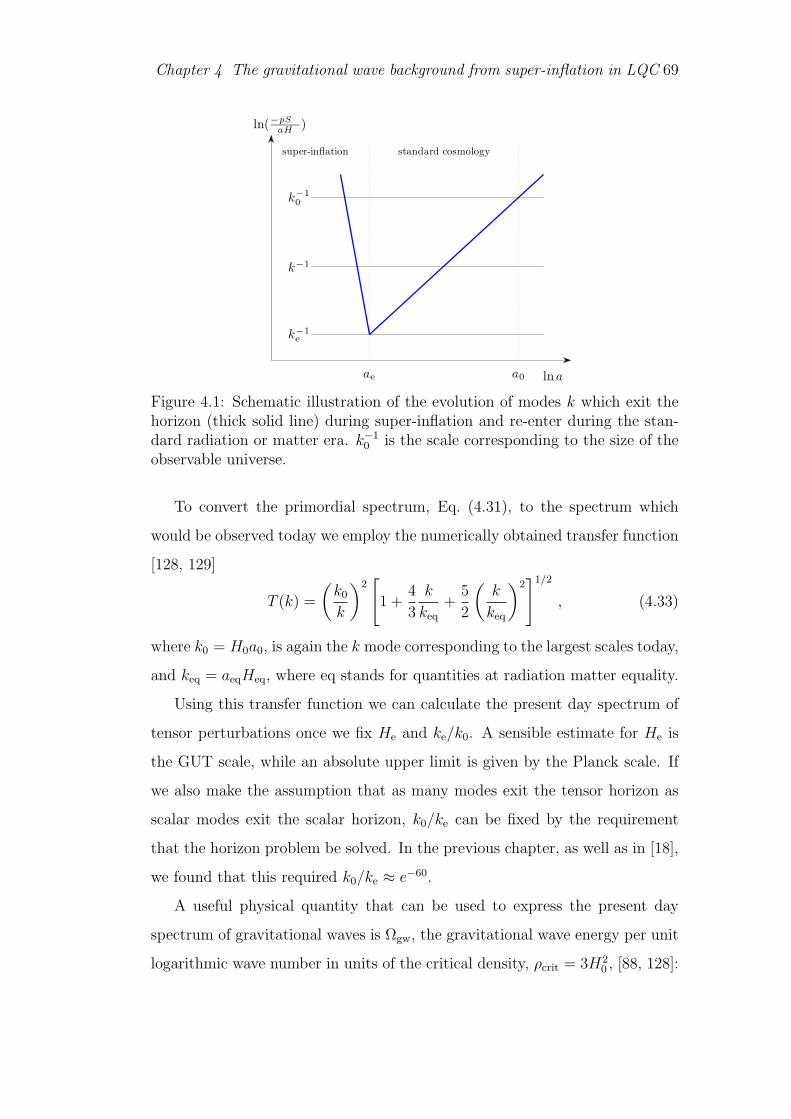
Chapter 4 The gravitational wave background from super-inflation in LQC 69
standard cosmologysuper-inflation
lna
ln(−pS
aH)
ae a0
k−1
0
k−1
k−1
e
Figure 4.1: Schematic illustration of the evolution of modes k which exit thehorizon (thick solid line) during super-inflation and re-enter during the stan-dard radiation or matter era. k−1
0 is the scale corresponding to the size of theobservable universe.
To convert the primordial spectrum, Eq. (4.31), to the spectrum which
would be observed today we employ the numerically obtained transfer function
[128, 129]
T (k) =
(k0
k
)2[1 +
4
3
k
keq
+5
2
(k
keq
)2]1/2
, (4.33)
where k0 = H0a0, is again the k mode corresponding to the largest scales today,
and keq = aeqHeq, where eq stands for quantities at radiation matter equality.
Using this transfer function we can calculate the present day spectrum of
tensor perturbations once we fix He and ke/k0. A sensible estimate for He is
the GUT scale, while an absolute upper limit is given by the Planck scale. If
we also make the assumption that as many modes exit the tensor horizon as
scalar modes exit the scalar horizon, k0/ke can be fixed by the requirement
that the horizon problem be solved. In the previous chapter, as well as in [18],
we found that this required k0/ke ≈ e−60.
A useful physical quantity that can be used to express the present day
spectrum of gravitational waves is Ωgw, the gravitational wave energy per unit
logarithmic wave number in units of the critical density, ρcrit = 3H20 , [88, 128]:
Chapter 4 The gravitational wave background from super-inflation in LQC 70
Ωgw(k) ≡ k
ρcrit
dρgw
dk=
1
6
(k
k0
)2
T 2(k)Ph , (4.34)
where the combination T 2(k)Ph represents the present-day gravitational wave
power spectrum; and we note that for its fixed values, the energy density varies
with k2. In general, if the k-dependence of the transfer function (4.33) is given
by kγ, the scale dependence of Ωgw will be k2+2γ+nt .
Figure 4.2 shows a plot of the present tensor abundance for a number
of choices of the parameter p, together with the strongest observational con-
straints from current and future experiments searching for gravitational waves
[88, 130]. Note that the gradient of the curves on large scales (i.e. γ → −2), is
−2 + nt; and on small scales (i.e. γ → −1), it will be nt. This is clearly seen
in Fig. 4.2 for the case of the standard inflation, where p → −1 from below,
where the curve appears almost horizontal for all frequencies f > feq, which
corresponds to the almost scale-invariance of gravitational modes in this case.
From the value of (aeqHeq)−1 = 14h−2Mpc, where h ≈ 0.7, one obtains the
corresponding frequency of feq = 10−15 Hz. f0 for today is similarly found
to be f0 = 10−18Hz. Since we have fixed He = 10−6, and we also find for
a radiation dominated universe aeqHeq
aeHe∝ ae
aeq∝ 10−23 (where we have used
1 + zeq = a0
aeq≈ 104), we obtain aeHe = 108, corresponding to the frequencies
in the region of fe = 108 Hz.
It can be seen from this figure that by relaxing the assumtion of He = 10−6,
corresponding to the GUT scale, one would effectively shift the intersection
point of the three lines to the left. Although this has the effect of bringing
the Ωgw of today (for p > −1) up on the vertical axis, the amplitude of tensor
fluctuations remains suppressed by quite a few orders of magnitude on the
CMB, compared to the standard inflationary case. This is a direct result of
the large blue tilt of the spectrum.

Chapter 4 The gravitational wave background from super-inflation in LQC 71
10−20
10−10
100
1010
10−60
10−40
10−20
100
CMB PULSAR LISA LIGO
BBO
BBN
f (Hz)
Ωgw(ω
,τ0)
Inverse triad corrections
p =−1p =−0.1p =−0.001
Figure 4.2: Predicted present abundance of gravitational waves produced dur-ing the super-inflationary phase of LQC with inverse volume corrections, as-suming that He = 10−6 in Planck units. The solid line corresponds to thestandard inflation abundance (n = r = 0). Also indicated are the presentbounds and future sensitivities.
4.3 Tensor dynamics with holonomy correc-
tions
We now turn our attention to the second set of effective equations, those which
arise from considering that holonomies are the basic operators to be quantised
in LQC.
The isotropic unperturbed dynamics is described, by the Friedmann equa-
tion [44, 51, 71, 50, 34, 53, 54]:
H2 =1
3a2ρ
(1− ρ
2σ
), (4.35)
which is modified from the classical equation by the inclusion of a −ρ2 term,
where σ = 3/(2γ2) is a constant in an exactly isotropic model, and where γ
is the Barbero-Immirzi parameter [36, 37]. This is identical to Eq. (2.16) first
introduced in chapter 2, but here is written in terms of conformal time, τ . We
are assuming either a flat universe or that the curvature term can be safely
neglected. Our interest here is in a scalar field dominated universe, and hence
Chapter 4 The gravitational wave background from super-inflation in LQC 72
ρ = φ′2/2a2 + V (φ). The scalar field equation of motion remains unchanged
from its classical form given by Eq. (3.56), which in terms of conformal time
can be written as
φ′′ + 2Hφ′ + a2V,φ = 0 . (4.36)
We stress that as we are studying inverse volume and quadratic corrections
separately, we do not include the D and S functions in the equations of motion.
The form of the evolution equation for tensor perturbations when holonomy
corrections are included has recently been derived to be [69]
h′′×,+ + 2Hh′×,+ −∇2h×,+ + TQh×,+ = 2ΠQ , (4.37)
where
TQ =a2
3
ρ2
2σ, (4.38)
ΠQ =1
2
ρ
2σ
(a2 ρ− φ′2
)h×,+ , (4.39)
are quantum corrections to the classical dynamics that become unimportant
when ρ ¿ 2σ. From here on we again drop the × and + subscripts as we did
in the inverse triad case.
4.3.1 Power-law solution and scale invariant scalar field
perturbations
We are interested in high density regimes where ρ approaches the bounding
value of 2σ. In this case, the term within brackets of Eq. (4.35) tends to
zero and the behaviour of the equations alters significantly compared with the
classical behaviour. Indeed in this regime we have H > 0 (seen from Eq. (2.17))
and for an expanding universe super-inflation takes place. In section 3.3 (and
also in [18]), we showed that in this regime there exists an approximate power-
law solution for a potential of the form V = 2σ − U0e−λφ (i.e. as given by
Eq. (3.61)). Moreover, this solution is an attractor as we demonstrated both

Chapter 4 The gravitational wave background from super-inflation in LQC 73
analytically and numerically in section 3.3 (also in [18]). The full background
cosmology solution is given by
a(τ) = A(−τ)p , (4.40)
φ′(τ) =√−2p(p + 1)
1
τ, (4.41)
V (τ) = 2σ − p(2p− 1)
(aτ)2(4.42)
where A is an arbitrary normalisation constant. λ and p are related through
λ2 = −2p + 1
p. (4.43)
Once again −1 < p < 0 corresponds to a universe undergoing super-inflation
(i.e. H > 0), and moreover the limit p → 0 from below leads to a scale-
invariant spectrum of scalar field perturbations, as seen from Eq. (3.91) dis-
cussed in section 3.3. Furthermore, as was the case for the super-inflationary
solution we studied in the presence of inverse volume corrections, only a small
number of e-folds are required to solve the horizon problem. In the previous
chapter we generalised the form of the potential that could be considered by
expanding about this solution, but for simplicity in this work we will consider
only this exact form.
We now turn our attention to the question of what spectrum of tensor
perturbations accompanies the scale-invariant spectrum of scalar field pertur-
bation in this version of super-inflation.
4.3.2 The primordial spectrum of tensor perturbations
We again follow the standard procedure for calculating the spectrum of ten-
sor perturbations. In our perfectly isotropic scenario, Eq.s (4.18) and (4.19)
remain unaltered. Imposing Eq. (4.20) then implies that h′ is canonically
conjugate to 2a2h such that
1
2h′(t, x),−a2
2h(t, y)
= δ3(x, y) . (4.44)

Chapter 4 The gravitational wave background from super-inflation in LQC 74
To quantise the system h and h′ are promoted to operators and Fourier
decomposed according to Eq. (4.10). Each hk mode satisfies the evolution
equation given by substituting Eq.s (4.38)-(4.39) into Eq. (4.37) during the
sacling solution:
h′′k + 2a′
ah′k +
[k2 − 4σ
3(−τ)2p − 2p(p + 1)
τ 2
]hk = 0 , (4.45)
where we have used ρ ≈ 2σ, and Eq. (4.41) has been substituted into Eq. (4.39).
This equation does not have an exact analytical solution 1. We study the dy-
namical behaviour by analysing this equation in some particular and physically
interesting limits. At early times (i.e. τ → −∞), we note that the second
term inside the brackets is more dominant than the third term. As the system
evolves in time, at late times (i.e. τ → 0−), the situation is reversed and the
third term dominates over the second. This is true for all modes. From our
discussion in section 3.4 we know that during the super-inflationary phase, the
term proportional to τ−2 increases by about e140 (from Eq. (3.107)), and the
term proportional to the square of the scale factor increases by about e140p
(from Eq. (3.108)). In the limit that p → 0, which is the case we are interested
in, this means that during the super-inflationary evolution the second term in-
side the brackets of Eq. (4.45) can be treated as a constant relative to the third
term. We, therefore, consider an effective wave number k2eff = k2 − 4σ
3(−τ)2p,
which introduces a shift in the wave number k, and we rewrite the mode equa-
tion in terms of this new parameter
h′′k + 2a′
ah′k +
[k2
eff −2p(p + 1)
τ 2
]hk = 0 . (4.46)
For very small scales (i.e. k →∞), we can use the approximation k2eff ≈ k2,
and following a similar method to what we did in the previous section, the
1This equation is different to what we quoted in [19], where the second term inside thebracket was mistakenly absent. In that paper we gave a full analytic solution for the equationwe had derived. Much of the analysis in this section is similar to the paper, but we alsomake comments on how the presence of a term proportional to the scale factor in the modeequation could be treated and interpreted.
Chapter 4 The gravitational wave background from super-inflation in LQC 75
solution to Eq. (4.46) is found to be
hk(τ) =1
H1/2a
√−p π H(2)ν (−kτ) , (4.47)
where
ν =1
2
√1 + 4p + 12p2 , (4.48)
where we have normalised the solution by the requirement that ak and a†k sat-
isfy the usual raising and lowering operator algebra while a2h and h′ satisfy
their commutation algebra, with only the forward moving solution being se-
lected in the asymptotic past (selecting the adiabatic vacuum). Note that this
normalisation has been done on the very small scales, where quantum fluc-
tuations are thought to be most important. We do not expect the difference
between keff and k to be significant in this limit.
Finally, utilising Eq. (4.12) and evaluating this expression in the limit that
the modes are outside the horizon (k < −H/p in this case), leads us to the
same expression for the primordial power spectrum (4.31), with the difference
that now ν is given by Eq. (4.48). The spectral index can clearly be seen to
be given by
nt ≈ 2− 2p ≈ 2 (4.49)
in the limit p → 0, and the amplitude fixed by He. We note here that in
cases where the dynamics of tensor perturbations could be represented by the
standard equation of motion and the evolution of the scale factor is given by
Eq. (4.40), having p → 0 will inevitably result in nt = 2. This has indeed
been shown to be true explicitly for the collapsing ekpyrotic scenario [88] and
for the evolution of a universe sourced by a phantom field [124]. In the full
Eq. (4.46), for the physically meaningful case of k2eff being a positive quantity,
there is a lower limit on the wave number k, which we denote as kmin and
is set by the largest value 4σ3
(−τ)2p can take. Since σ = 32γ2 depends on the
fundamental loop parameter γ, which is of order unity [38, 39], the limiting
quantity is the size of the square of the scale factor. (−τ)2p is largest at the

Chapter 4 The gravitational wave background from super-inflation in LQC 76
end of the super-inflationary era, and for all modes much greater than this
value the argument and the analysis above remains valid. One thing to notice
is that for modes of the order of the scale factor, in calculating the spectral
tilt, we have from Eq. (4.12)
Ph ∝ k3 k−2νeff . (4.50)
For the scaling solution we have been considering, in the limit of p → 0,
from Eq. (4.48) we have ν → 1/2. It is clear that the value of the power spec-
trum of (4.31) is only approximately valid when k is close to the value by which
it is shifted, and in fact the power spectrum (4.50) will pick up modifications
in lower powers of k. The spectral tilt of approximately 2 will still be the lead-
ing order result for this scenario. It is not physically meaningful to consider
frequencies lower than kmin. We, therefore, make the assumption that this
sets the maximum scale of the universe for which Eq. (4.46) holds. Whilst the
combination k2− 4σ3
(−τ)2p is much less than τ−2 at late times on this scale, the
spectral tilt calculated above is correct. This does not mean that the universe
can not grow beyond this scale, but rather that our results here suggest we can
not make any predictions on primordial gravitational waves corresponding to
scales greater than kmin. We, thus, assume that for the purpose of our study
we are only dealing with modes that are physically meaningful if Eq. (4.46) is
to hold.
At this point, making some reasonable assumptions, we can proceed, as we
did for the solution in the inverse triad case, to calculate the present day spec-
trum of gravitational wave perturbations using the transfer function Eq. (4.33).
We show the abundance of tensors in Fig. 4.3 and note that the result is very
similar to the inverse volume case.

Chapter 4 The gravitational wave background from super-inflation in LQC 77
10−20
10−10
100
101010
−80
10−60
10−40
10−20
100
CMB PULSAR LISA LIGO
BBO
BBN
f (Hz)
Ωgw(ω
,τ0)
Holonomy corrections
p =−1p =−0.1p =−0.001
Figure 4.3: Predicted present abundance of gravitational waves produced dur-ing the super-inflationary phase of LQC with holonomy corrections. The solidline corresponds to the standard inflation abundance. Also indicated are thepresent bounds and future sensitivities.
4.4 Discussion
We conclude that super-inflation in both versions of the corrections in LQC
predicts a strong blue spectrum of gravitational waves, hence, their abundance
is strongly suppressed on the large scales and it is many orders of magnitude
smaller than the value predicted in the standard inflationary scenario. In the
case of the holonomy corrections, we have the extra feature of a maximum scale
being introduced for which the calculation of the spectral tilt of the gravita-
tional waves can be performed. In our analysis we have made the assumption
that the scales we can probe today are smaller than this value. This is a new
result and has not been mentioned elsewhere in the literature.
It is now important to discuss our results in the light of other investigations
in the literature. In particular, it is claimed in Ref. [131] that the abundance
of gravitational waves generated during super-inflation under inverse volume
corrections is above the current bounds. We note however that the authors did
not consider the evolution of the background in a scaling solution and the S(a)

Chapter 4 The gravitational wave background from super-inflation in LQC 78
correction was not used. Moreover, the full expression for the tensor pertur-
bations was obtained more recently [69] and therefore it was not used in that
work. In a more recent analysis [126] focusing on the holonomy corrections, it
is also found, like in our work, that the spectrum of gravitational waves must
be blue. However, a scaling solution was not used and the expansion of the
universe was assumed to be close to de Sitter, hence, a direct comparison with
our work is in fact not possible.
We have highlighted the similarities between our predictions of tensor per-
turbation spectral index in the context of LQC and those obtained in the
ekpyrotic collapse models and also when the universe is sourced by a phantom
field.
One needs to be cautious about making general conclusions in the context
of LQC, as the theory is currently far from complete. As mentioned previously,
the introduction of inhomogeneities in the small a regime is likely to break the
assumption of an isotropic universe. Attempts are being made to gain better
understanding of this region [125]. Moreover, there is the possibility that
higher order perturbative correction terms could play a role, or that quantum
backreaction might significantly modify the background dynamics [132].
Despite the ambiguities and uncertainties in the theory, if we were to make
observational claims for the scaling solutions we have considered in the current
state of LQC, it would be that if gravitational waves are observed, they would
rule out this scenario of superinflation in LQC as it stands.

Chapter 5
Field perturbations: LQC
mapped to Braneworlds
5.1 Introduction
A successful and consistent picture of the evolution of the universe is provided
by the standard model of cosmology based on General Relativity. It is widely
believed that by approaching the validity limit of GR, this picture will be
modified. One expects this to happen at the high energy levels of the very
early universe, and modifications to arise in the Friedmann equations when
the curvature of the universe is quite high. A theory of Quantum Gravity
is expected to shed light on the nature of these corrections by probing the
quantum properties of spacetime near the Big Bang. There have been a number
of attempts at formulating such a fundamental theory, most popular of which
are either motivated by higher dimensions and are related to string/M-theory
(e.g. [73, 74]), or are inspired by Loop Quantum Gravity (LQG) based on
four spacetime dimensions [14]. We will consider braneworld cosmologies in
the former class of theories and we limit ourselves to the LQC model in the
latter class.
We discussed in Chapter 2 the setup of simple braneworld cosmologies and
the types of corrections they can introduce to the Friedmann equations. In
the course of the previous chapters we have also reviewed in detail the nature
79
Chapter 5 Field perturbations: LQC mapped to Braneworlds 80
of modifications that arise in the context of LQC. Despite the different under-
lying physical pictures in these scenarios, since they both ultimately aim to
describe what one observes in the universe, and assuming both approaches are
correct in the modifications they introduce beyond the standard description
of GR, we are interested in finding out how one could relate their predictions
in a quantitative fashion. The work of [20] has considered a possible map
between the inverse volume corrections of LQC and typical braneworld cos-
mologies. This correspondence maps the background cosmologies of the two
sets of models, and since the number of free parameters on both sides are un-
equal, a particular LQC model can be mapped to a class of braneworld models
and visa versa. The map is produced by demanding that both cosmologies
result in the same effective Hubble parameter. Since this is a typical parame-
ter that could be measured, any physically viable theory is expected to make
the correct prediction for it. By making the assumption that both theories
under investigation are physical descriptions of our universe, to relate their
predictions at the cosmological background level, one obtains a map between
the two in this way [20]. Notice that such a map does not prove if/how these
theories may be equivalent.
The aim of this chapter is to investigate whether this map would also link
other physically measurable quantities predicted through the corrections these
theories introduce to our understanding of cosmology. We begin by reviewing
the outline of the calculations of [20] for the more general LQC model described
in Chapter 2. Considering the general modifications made to the Friedmann
equations in braneworld-inspired cosmologies, we derive the correspondence
map at the cosmological background level in section 5.2. We will proceed in
section 5.3 to map the LQC model of the inverse triad corrections to a class
of braneworld cosmologies at the background level using phase space analy-
sis. Since stability is an important physical property in cosmology, we check
and see if this property is mapped directly across from LQC to braneworlds.
The scale-dependence of the scalar field perturbations in the braneworld cos-
mologies is derived in section 5.4, followed by a comparison made in section
Chapter 5 Field perturbations: LQC mapped to Braneworlds 81
5.5 between these perturbations and the near scale-invariant perturbations we
have presented in the previous two chapters in the case of the LQC model.
We do this to investigate whether the two cosmologies also correspond to one
another at the perturbation level. We will conclude in section 5.6.
5.2 Relating LQC and Braneworld cosmolo-
gies at the background level
A constraint equation relating braneworld cosmologies and LQC-inspired cos-
mologies at the background level was derived in [20]. For our purposes, we
derive a more general form for this equation, when considering the inverse vol-
ume corrections to the Friedmann equation and the equation of motion in LQC
are given by Eqs. (2.15) and (2.12), also reproduced below for easy reading:
H2l =
κ2
3S
(φ2
2D+ V (φ)
), (5.1)
φ + 3Hl
(1− 1
3
d ln D
d ln a
)φ + DV,φ = 0 . (5.2)
In these equations, φ and V are the LQC scalar field and scalar potential,
respectively, as before.
The braneworld modifications to the classical Friedmann equation and the
equation of motion for the homogeneous scalar field, χ, are such that
H2b =
κ2
3ρχL2(ρχ) , (5.3)
χ + 3Hbχ + W,χ = 0 , (5.4)
where L2(ρχ) represents the quantum gravitational modifications in braneworld
models. We have already mentioned the Randall-Sundrum model in section
2.3, where L(ρχ) =√
1 + ρχ
2σ(from Eq. (2.18)), and the Shtanov-Sahni model,
where L(ρχ) =√
1− ρχ
2σ(from Eq. (2.31)). Other examples and different
Chapter 5 Field perturbations: LQC mapped to Braneworlds 82
forms of the function L(ρχ) can also be found in [133]. χ and W represent
the scalar field and its potential in the braneworld cosmology, respectively;
and ρχ = χ2
2+ W (χ) is the energy density associated with the homogeneous
scalar field, χ. For both cosmologies we have made the assumption that the
curvature term is subdominant. These equations are valid in the absence of
any fluid, where the energy density is dominated by the scalar fields.
By allowing the evolution of both systems to be governed by the same
Hubble parameter (i.e. Hl = Hb), motivated by the reasons mentioned above,
we obtain the constraint equation
2φ2
φ2 + 2DV
(1− 1
6
d ln D
d ln a
)− r
3= −1
3
d ln (ρχL2(ρχ))
d ln a. (5.5)
It is easy to check that the left hand side of Eq. (5.5) can be written as2(1−n
6 )1+2c
− r3, where c = DV
φ2 is a constant when considering scaling solutions.
After substituting these into the constraint equation and integrating, we find
that, up to a constant
ρχL2(ρχ) = an−61+2c
+r. (5.6)
Using Eq. (5.3), the scale factor of the braneworld cosmology is found as a
function of conformal time, τ , to be
a = A0(−τ)α , (5.7)
where α is defined as
α ≡ −2(1 + 2c)
(1 + 2c)(2 + r) + n− 6, (5.8)
and A0 =(−1√3α
)α
is a positive constant. Notice that this is consistent with an
expanding universe, where one requires α < 0. As an ansatz, let us assume we
can write the braneworld scalar field and its potential as power-law functions:
χ = χ0(−τ)Λ, W = W0(−τ)σ. (5.9)
Chapter 5 Field perturbations: LQC mapped to Braneworlds 83
where χ0 and W0 are constants. By substituting Eq. (5.9) into Eq. (5.4), and
requiring every term to evolve with the conformal time in the same way, we
obtain the following relations:
σ = 2(Λ− 1− α), 2W0A20 = −Λ2χ2
0
Λ− 1 + 2α
Λ− 1− α. (5.10)
We note that the first of these relations is equivalent to a scaling require-
ment on the braneworld cosmology, meaning the same equation can be found
for σ if we demanded χ2/W to be a constant. This is a desirable outcome and
we will discuss the stability properties of these solutions later in this chapter.
By substituting our ansatz (5.9) into Eq. (5.3), we find that the general form
of the braneworld modifications made to the standard cosmology satisfying
the constraint equation (5.5), is
L2(ρχ) ∝ ρ−Λ
Λ−1−αχ . (5.11)
This is an important result and it suggests that the Hubble parameter
evolves as a power-law function of the scalar field energy density. Since L2(ρχ)
represents the high energy corrections made to the standard cosmology, we
expect it to become more significant as we go back in time towards the Big
Bang, where the energy density of the universe would have been much greater
than its value later on in the evolution of the universe. Let us consider the case
where L2(ρχ) = ρmχ , where m > 0. In this case using Eq.s (5.3), (5.4),(5.10),
and (5.11), we obtain
Λ =m(1 + α)
1 + m, (5.12)
χ20 =
2(3α2)−αm−11+m (1 + m)
3αm2(1 + α), (5.13)
W0 =(3α2)
1+α1+m (2α− 1 + 3αm)
3α(1 + m). (5.14)

Chapter 5 Field perturbations: LQC mapped to Braneworlds 84
Notice that since α < 0, W0 is positive definite, and the form of the poten-
tial as a function of the scalar field is derived, using Eq. (5.9), as W ∝ χ−2/m.
i.e. W (χ) is a positive, inverse power-law potential.
Notice further that by substituting Eq. (5.12) into the expression for the
rate of change of the Hubble parameter
H =1
2χ2L2(ρχ)
1 + α
Λ− 1− α, (5.15)
we find that H < 0, and using the behaviour of our braneworld scale factor in
Eq. (5.7), this implies α < −1.
5.3 Stability analysis of the Braneworld cos-
mology
There is a class of cosmological solutions, referred to as the ‘scaling solutions’,
which are usually considered to have the important desirable property of de-
scribing asymptotic late time behaviour of cosmological backgrounds, and are
often found to be stable attractors [95, 96, 97, 153, 110]. Our focus here is
based on such solutions in the context of the modified braneworld cosmologies
we are considering. We saw in Chapter 3 the form of the background cosmol-
ogy which yields scaling solutions in the semi-classical regime of LQC, and a
stability analysis was also carried out on these solutions in section 3.2.3. This
section is dedicated to using a similar procedure to determine the late time
behaviour and stability criteria for the corresponding braneworld cosmology.
By employing the phase space analysis method developed in [149, 150] for such
scenarios, we proceed by defining the following two parameters:
x ≡ χ√2ρχ
, y ≡√
W√ρχ
. (5.16)
It is then easy to show that Eq.s (5.3)-(5.4) can be written in terms of these
parameters in the following form:

Chapter 5 Field perturbations: LQC mapped to Braneworlds 85
x,N = −3x(1− x2) +
√3
2λy2 , (5.17)
y,N =
√3
2λxy + 3x2y , (5.18)
λ,N = −√
6(Γ− 1)λ2x + 6λd ln L(ρχ)
d ln ρχ
x2 , (5.19)
where λ and Γ are defined as
λ ≡ − 1
L(ρχ)
W,χ
W, Γ ≡ W,χχW
W 2,χ
. (5.20)
In the model under consideration,
λ,N = −√
6(Γ− 1)λ2x + 3mλx2 . (5.21)
The x and y parameters defined here, in the absence of any fluid, are subject
to the constraint equation
x2 + y2 = 1. (5.22)
Taking λ to be constant, and substituting this constraint equation into Eq. (5.17),
makes Eq. (5.18) redundant, and together with Eq. (5.21) results in an au-
tonomous system with three fixed points:
xc1 = 1 , yc1 = 0 , Γc2 = 1 +
√3/2
λm , (5.23)
xc2 = −1 , yc2 = 0 , Γc2 = 1−√
3/2
λm , (5.24)
xc3 =λ√6
, yc3 =
√1− λ2
6, Γc3 = 1 +
m
2, (5.25)
The first two points correspond to kinetic energy dominated solutions, and
the third point is a scaling solution, where the kinetic and the potential ener-
gies of the scalar field scale together throughout the evolution of the universe.
In order to analyse the late time behaviour and stability conditions for our

Chapter 5 Field perturbations: LQC mapped to Braneworlds 86
system, we study the nature of these fixed points. We do this by linearising
Eq.s (5.17) and (5.21) about the fixed points and determining the correspond-
ing eigenvalues in each case, using the methods outlined in Chapter 2. The
M-matrix for these equations is found to be
M =
−3−√6xλ + 9x2 −
√32(x2 − 1)
−√6(Γ− 1)λ2 + 6mλx −2√
6x(Γ− 1)λ + 3mx2
(5.26)
admitting the following eigenvalues for the kinetic energy dominated fixed
points
ωc1+ = 6−√
6λ , ωc1− = −3 , (5.27)
ωc2+ = 6 +√
6λ , ωc2− = −3 . (5.28)
The first of these is stable for λ ≥ √6, and the second is stable when
λ ≤ −√6. The eigenvalues of the scaling solution are
ωc3+ = 0 , ωc3− = −3 , (5.29)
which means this solution is unconditionally stable. By considering the scaling
solution, we observe that the valid range of λ for the existence of these solutions
is given by λ2 ≤ 6. In fact, as the scalar field rolls down its positive inverse
power-law potential, initially, the kinetic energy dominated solution is the
stable fixed point, where the potential is steep. Thereafter, the potential drops
and flattens, where the scaling solution then becomes the late-time attractor.
We have demonstrated that the scaling solutions of the corresponding
braneworld scenario to the LQC model considered in this chapter are also
late time attractors. This is a desirable result, since stability can be viewed
as a physical property of our universe and the fact that both cosmologies un-
der study, related via the constraint Eq. (5.5), are asymptotically stable is
encouraging.

Chapter 5 Field perturbations: LQC mapped to Braneworlds 87
5.4 Power Spectrum of the perturbed field
In this section we proceed to calculate the vacuum fluctuations of the scalar
field, χ. We will then make a comparison between our results here and the
spectrum of the scalar field perturbations calculated in Chapter 3. We start
by splitting the field into homogeneous and perturbation parts: χ → χ + δχ.
The perturbation in the field, δχ, satisfies
¨(δχ) + 3H ˙(δχ) + (W,χχ −∇2)(δχ) = 0 , (5.30)
which upon introducing u = aδχ, can be written as
u′′ +(−∇2 + m2
eff
)u = 0 , (5.31)
where
m2eff = −a′′
a+ W,χχa2 . (5.32)
Following the general methods employed in this type of analysis, first de-
scribed in chapter 3, we quantise u by promoting it to an operator u. An
appropriate conjugate momentum πu can also be defined such that a similar
relation to Eq. (3.27) holds in this case. Decomposing u in Fourier modes, uk,
gives Eq. (3.29), written here for easy reading:
u(τ,x) =
∫d3k
(2π)3[uk(τ)ak eik.x + u∗k(τ) a†k e−ik.x] , (5.33)
where the modes satisfy the mode equation
u′′k +(k2 + m2
eff
)uk = 0 . (5.34)
The power spectrum of these modes can then be calculated from the defi-
nition
Pu ≡ k3
2π2|uk|2 . (5.35)
Chapter 5 Field perturbations: LQC mapped to Braneworlds 88
The general solution to Eq. (5.34) is given by
uk(τ) =
√π
2|2 + np|(d1
√−τ H(1)|ν| (x) + d2
√−τ H(2)|ν| (x)
)(5.36)
whenever meffτ is constant, and where
ν = −√
1− 4 m2eff τ 2
2. (5.37)
H(1)|ν| (x) and H
(2)|ν| (x) are Hankel functions of the first and second kind, respec-
tively. Following the procedure outlined in the previous two chapters, the
constants d1 and d2 can be chosen such that only the forward moving wave is
chosen. In the long wavelength limit, the power spectrum yields
Pu ∝ k3−2|ν| (−τ)1−2|ν| . (5.38)
We expect to have scale-invariance when this power spectrum is indepen-
dent of k. In order to quantify the scale dependence properties of the field
perturbations, we define a set of slow-roll parameters; and produce an expan-
sion in these parameters describing the deviation of our field perturbations
from exact scale-invariance.
We define our first slow-roll parameter as
ε ≡ 1
2λ2 =
1
2
1
L2(ρχ)
(W,χ
W
)2
, (5.39)
and we will soon explain that this is an appropriate parameter to choose for
a slow-roll inflationary scenario in these models. For the model we have been
considering, this parameter can be written as
ε =1 + α
α(1 + m), (5.40)
or alternatively, we have that α = 1(1+m)ε−1
. The background cosmology can
then be written in terms of these parameters:
Chapter 5 Field perturbations: LQC mapped to Braneworlds 89
a = A0(−τ)1
(1+m)ε−1 , (5.41)
χ′ = −√
2ε
(1 + m)ε− 1
[3
((1 + m)ε− 1)2
] −m2((1+m)ε−1)
(−τ)mε
(1+m)ε−1−1 ,(5.42)
W =3− ε
((1 + m)ε− 1)2
[3
((1 + m)ε− 1)2
]− m1+m 1
(aτ)2
1+m
. (5.43)
By substituting Eq. (5.41) - (5.43), into Eq. (5.32), we find
m2effτ
2 =3α(α + 1)(1 + m)2 − (mα− 1)(m(α− 1)− 2)
(1 + m)2. (5.44)
It is then evident from Eq. (5.37)-(5.38) that scale-invariance is obtained
in the braneworld scenario for α → −1, and α → − m(2m+3)2m2+6m+3
. The latter is
outside the valid range of α (for our assumption of m > 0), but the former
falls within the acceptable range, and corresponds to larger values of the scalar
field, where the potential is flat and the field is slowly rolling down. As we
evolve towards a stable scaling solution, we expect this behaviour of the field
to lead to slow-roll inflation. The limit of α → −1 also implies that ε ¿ 1,
and it can consequently be treated as a conventional slow-roll parameter.
We would like to be able to generalise our argument for the potentials
which are not of the exact form that give rise to the scaling solutions we have
discussed, but approach these solutions asymptotically. We can account for
small deviations from exact solutions by allowing the slow-roll parameters to
be time dependent, but we also impose the condition that they are only slowly
varying with time. It then follows from differentiating Eq. (5.39) that
ε′ = −(2ε)3/2 L(ρχ)η(τ)χ′ , (5.45)
where the second slow-roll parameter, η, is defined as
η(τ) ≡ 1 +W
W,χ
L(ρχ),χ
L(ρχ)− W,χχW
W 2,χ
. (5.46)
Chapter 5 Field perturbations: LQC mapped to Braneworlds 90
It is also easy to show that η′ = −√2ε L(ρχ)ξ2χ′, where
ξ2 ≡ W,χχW
W 2,χ
(1 +
W,χχχW
W,χχW,χ
− 2W,χχW
W 2,χ
)
− WL,χ
W,χL
(1 +
L,χχW
L,χW,χ
− L,χW
LW,χ
− W,χχW
W 2,χ
). (5.47)
By imposing the variations of ε and η with time (i.e. d ln εd ln a
≈ 4εη, and
d ln ηd ln a
≈ 2 ε ξ2
η) to be negligible, one observes that η and ξ2 should be very
small. We will drop ξ2 and higher orders in the perturbation expansion in
what follows.
In order to quantify the spectral tilt of the scalar field perturbations, we
substitute the appropriate slow-roll parameters into the expression for the
effective mass Eq. (5.32). The deviation from exact scale-invariance is given,
from Eq. (5.38), by ∆ns = 3 −√
1− 4m2effτ
2. After expanding to first order
we find
∆ns ≈ 2ε . (5.48)
Clearly, when ε ¿ 1, near scale-invariance is achieved. This is in line with
the limit of α → −1 for the case of our late time scaling solution.
5.5 Relating LQC and Braneworld cosmolo-
gies at the perturbation level
In this section we make a comparison between the spectral tilt of perturbations
of the scalar field, φ, in LQC given by Eq. (3.49) and the braneworld scalar
field perturbations. In order to establish if the two cosmologies are related
at the perturbation level in the same way they correspond to each other at
the classical level, we ask the following question. When the scalar field power
spectrum of the braneworld cosmology is rewritten in terms of the LQC para-
meters, would the scale-invariance condition of our LQC model also result in

Chapter 5 Field perturbations: LQC mapped to Braneworlds 91
scale-invariance in this rewritten expression? We begin by writing Eq. (5.48)
in terms of the LQC parameters. In doing so, we first substitute the result
of the correspondence relation between the braneworlds and the LQC model
derived earlier in the form of Eq. (5.8) into Eq. (5.40). Eq. (5.48) then becomes
∆ns ≈ −r(1 + 2c) + n− 6
(1 + 2c)(1 + m), (5.49)
where c = DV/φ2 is a constant for the scaling solution considered in our
previous chapters. We now refer to the model we considered in the context of
LQC in chapter 3. By assuming we operate in the semi-classical regime (i.e.
D = D∗an), and setting D∗ = 1 without loss of generality, we can evaluate c
from Eqs.(3.20)-(3.21), and find
c =112
(n− 6)2 − εLoops
2εLoops
, (5.50)
where the subscript Loops refers explicitly to the LQC model. Rewriting
Eq. (3.19), we obtain an expression for εLoops:
εLoops = −(n− 6)(2 + p(2 + r))
12p, (5.51)
where p describes how the LQC scale factor behaves through Eq. (3.18). By
substituting this into Eq. (5.50), the expression for the braneworld scalar field
perturbations derived above in Eq. (5.49) becomes
∆ns ≈ 2(1 + p)
p(1 + m), (5.52)
which includes the LQC parameter p. We note here that in the limit p → 0,
the scalar field power spectrum in the braneworld cosmology blows up; but, as
shown in Chapter 3, this is indeed the limit of p for which scale-invariance is
obtained in LQC. This discrepancy needs to be examined more closely to gain
better understanding.
We have seen that by perturbing the scalar field χ, (i.e.χ → χ + δχ), the

Chapter 5 Field perturbations: LQC mapped to Braneworlds 92
perturbations satisfy Eq. (5.30). From Eq. (5.20), W,χχ can be written as
W,χχ = Γλ2WL2(ρχ) , (5.53)
which upon using the definition of y in Eq. (5.16) becomes
W,χχ = Γλ2y2ρχL2(ρχ) . (5.54)
For the scaling solution described by (5.25), we have
W,χχ = 3λ2(1 +m
2)(1− λ2
6)H2 , (5.55)
and once we employ the definition of εBranes in (5.39), it gives
W,χχ = 6H2(1 +m
2)εBranes(1− εBranes
3) , (5.56)
where the subscript Branes has been introduced to distinguish the slow-roll
parameters of each model explicitly. Similarly, for the LQC model the pertur-
bation equation of the scalar field, φ, is given by Eq. (3.22), which for easy
reading and flow of our line of argument is also given below in terms of cosmic
time, t.
¨(δφ) + 3H(1− n
3) ˙(δφ) + D(V,φφ −∇2)(δφ) = 0 , (5.57)
where we have assumed we are working in the semi-classical regime (i.e. D ∝an). V,φφ for our scaling cosmology is calculated through a similar method
outlined above, to be
V,φφ =6H2
DεLoops
[1− εLoops
3+
(n− r)(1− n−r
6
)
εLoops
+n
12(1− n
6
)]
. (5.58)
Let us start our investigation into the discrepancy by writing the LQC
scalar field, φ, in terms of the braneworld scalar field, χ. Since the core-
spondence relation derived in this chapter is based on demanding the Hubble
parameters of both models to be equal, the behaviour of the scale factors would
Chapter 5 Field perturbations: LQC mapped to Braneworlds 93
also be identical, up to a constant. Therefore, from Eq.s (3.18) and (5.7) we
have
p = α . (5.59)
From the dependence of the scalar field, φ, on conformal time for the scaling
solution in LQC [100, 18]
φ = φ0(−τ)((n−r)α/2) , (5.60)
where φ0 is a constant, and using Eq. (5.9), we have
φ = C χγ, (5.61)
where γ = (n−r)α(1+m)2m(1+α)
, and C = φ0
χγ0. By considering small variations in the
scalar fields, we will then have
(δφ) = Cγχγ−1(δχ) (5.62)
˙(δφ) = Cγ[(γ − 1)χγ−2χ(δχ) + χγ−1 ˙(δχ)
](5.63)
¨(δφ) = Cγ(γ − 1)[(γ − 2)χγ−3χ2(δχ) + χγ−2χ(δχ) + χγ−2χ ˙(δχ)
](5.64)
+ Cγ[(γ − 1)χγ−2χ ˙(δχ) + χγ−1 ¨(δχ)
]. (5.65)
Substituting these into Eq. (5.57) and upon using the expression for V,φφ
given by (5.58), we find the corresponding braneworld perturbation equation
for the case where Eq. (5.61) is satisfied, as
¨(δχ) + 3H
(1− n− r
3+
2Λ(γ − 1)
3α
)˙(δχ) +
[6H2 (qL + µ)−D∇2
](δχ) = 0 ,
(5.66)
where µ = Λ(γ−1)6α2
(Λ(γ − 1)− 1− α− 3α(1− n
3)), and qL is given by

Chapter 5 Field perturbations: LQC mapped to Braneworlds 94
qL = εLoops
[1− εLoops
3+
(n− r)(1− n
6
)
εLoops
+n− r
12(1− n
6
)]
. (5.67)
Let us remind ourselves that for the LQC and the braneworld models con-
sidered here to correspond to one another at the background level, the con-
straint Eq. (5.5) must hold. If they are also to correspond to one another at
the perturbation level, we expect Eq. (5.66) to be equivalent to Eq. (5.30),
which was derived independently for the braneworld scenario. This implies
the following two criteria must be met simultaneously:
2Λ(γ − 1)
3α− n− r
3= 0 , qB = qL + µ , (5.68)
where from Eq.s (5.30) and (5.57), qB = (1 + m2)εBranes(1 − εBranes
3) . Using
Eq. (5.12) and the form of γ given above, the first of these criteria can be shown
to be satisfied either for m = 0, which corresponds to the classical cosmology
case without the introduction of any quantum gravitational corrections; or
when α → −1, which is the case for our braneworld scaling solution considered
here. The latter is the case we are interested in.
The second of the criteria above, in the limit α → −1, implies that
qB ≈ qL +n
12(3− n
2) . (5.69)
Note that despite the forms of qB and qL being similar, they differ from
one another by orders of magnitude. In LQC, qL is very large due to the scalar
field potential, V , being very steep and consequently, the ‘slow-roll’ parameter,
εLoops, has a huge value. In the braneworld cosmology, however, qB is of the
order of εBranes, which is the slow-roll parameter and is very small due to the
nearly flat scalar field potential, W , in the region where the scaling solution is
a stable attractor. Thus, Eq. (5.69) is not satisfied unless n is very large, and
severely fine-tuned. This is not practical, as although there is no upper bound
specified for the quantisation parameter, n, in LQC, the highest feasible value

Chapter 5 Field perturbations: LQC mapped to Braneworlds 95
in the literature is close to 12 [48].
5.6 Discussion
It turns out that by imposing the Hubble parameter to be identical for the
inverse volume corrected LQC and the braneworld cosmology through applying
the constraint equation (5.5), it is not possible to obtain the same behaviour of
the scalar field perturbations in the two cosmologies when we consider scaling
solutions. The fundamental reason for this is the fast-roll nature of inflation
in the semi-classical regime of LQC which is obtained in the limit of the scale
factor growth parameter, p → 0. By asking the Hubble parameters in both
cosmologies to be identical, we are implicitly carrying this parameter, without
any modification, across to the braneworld cosmology. This parameter has
been denoted by α in the braneworld cosmology, and in fact, it is easy to show
that α = p for this correspondence to hold.
We showed in Chapter 3 that in the semi-classical region of LQC we have
a super-inflationary era irrespective of the form of the potential. It is easily
shown that the parameter space of p for which super-inflation is obtained is
−1 < p < 0, and it is in this range of p that one expects scale-invariance.
However, we have also shown here that this is outside the allowed range of α
in the braneworld cosmology we have investigated. Therefore, the inflationary
regimes of the two cosmologies do not map onto one another. It is for this
fundamental underlying reason that we do not see a correspondence between
the scale invariance criteria of the two models.
We realise that in order to be able to compare theory predictions with
observations, one would ideally like to be considering the curvature perturba-
tions. However, this has not been the primary aim of this chapter. Our main
purpose has been to compare the LQC and the braneworld cosmologies at the
perturbation level; and as discussed in Chapter 3, our current knowledge about
the metric perturbations in LQC is incomplete. This is why we concentrated
on calculating the scalar field fluctuations in LQC. We then proceeded to focus

Chapter 5 Field perturbations: LQC mapped to Braneworlds 96
on the power spectrum of the braneworld scalar field perturbations in order to
make a fair comparison between the two models.
Other attempts have also been made in the literature to identify pos-
sible correspondences between LQC and braneworld cosmologies. Despite
the apparent similarity between the form of LQC modified cosmologies due
to holonomy corrections given by Eq. (2.16) and the Shtanov-Sahni model,
Eq. (2.31), no formal link has been proposed to relate these models. However,
in [111] a thorough investigation has led to obtaining a dual relationship be-
tween the holonomy corrected model of LQC and the Randall and Sundrum
(R-S) model at the level of background scaling solutions. This is a result that
theoretically links the brane tension in the R-S model to the fundamental loop
parameter, γ. This can be done by assuming the energy levels below which
the Hubble parameter is not well defined are of similar magnitudes. In [135]
an independent line of study has led to a similar result relating the holonomy
corrections in LQC to the R-S model of cosmology by considering a deformed
Heisenberg algebra.
These maps have been considered for a perfectly isotropic and homoge-
neous universe, but there is no fundamental reason why this property should
be maintained at extremely high energy densities of the very early universe,
where these corrections would be significant. It would be interesting to see
how introduction of inhomogeneities and anisotropy alters such a result. In-
vestigating the behaviour of perturbations to see if the same map links both
models at the level of fluctuations would also shed light on the strength of
such a relationship. This task is beyond the scope of our investigation in this
chapter for the models we have discussed in the context of holonomy corrected
LQC scenario.

Chapter 6
Dynamics of a scalar field in
Robertson-Walker spacetimes
6.1 Introduction
Scalar fields have played a very important role in modern cosmology. Today’s
observed acceleration of the universe, for example, may be explained by the
dynamics of a scalar field (for a review, see [136]). The scenarios proposed to
solve the initial conditions of the standard Big Bang theory such as inflation
[22, 25, 26], pre-big bang [137, 138, 139], and the ekpyrotic/cyclic [80, 83]
scenarios also usually require a scalar field. One of the aspects which makes
these scenarios interesting is the existence of attractor solutions which implies
that the dynamical system becomes insensitive to the initial conditions. A
class of such attractor solutions is referred to as scaling solutions, where the
energy density can be divided into contributions which scale with one another
throughout the evolution of the universe. Investigating the nature of scaling
solutions allows one to understand the asymptotic behaviour of a particular
cosmology and helps determine whether such behaviour is stable or just a
transient feature.
In a spatially flat Friedmann-Robertson-Walker (FRW) universe filled with
a perfect fluid and a canonical scalar field, such scaling solutions are obtained
through a simple exponential potential [96]. The attractor behaviour in this
system has been analyzed extensively [140, 141, 142, 143, 144]. More recently
97

Chapter 6 Dynamics of a scalar field in Robertson-Walker spacetimes 98
they have been obtained for a wide class of modified cosmologies proposed
by fundamental theories. The cosmologies include those with a non-minimally
coupled scalar field [145, 146, 147, 148], braneworld cosmologies [149, 150, 151,
152, 153, 154], loop quantum cosmology, [63, 20, 18], and phantom cosmology
[155].
Fundamental theories may introduce modifications to the Friedmann equa-
tion in various models that may or may not be of a similar form. Since the
stability of the background cosmology is understood to be a desirable prop-
erty, the pragmatic approach is to accommodate such modifications in the
phase space analysis of the standard dynamical system. For the case of a flat
FRW universe, the analytical method of obtaining the scaling solutions has
been extended to a general set-up, where the Hubble parameter is given either
by an arbitrary power [158, 159] or an arbitrary function [110] of the total
energy density.
According to the latest results of WMAP5 [17], although limits being placed
on the flatness of our observable universe are squeezing the possible outcomes,
−0.063 < Ωk < 0.017, there is still the possibility that we live in a spatially
curved FRW universe. It is appropriate, therefore, to investigate the conse-
quences of curvature on the stability of the background cosmology.
In this chapter, using the method developed in [110] in the context of
braneworld corrections made to the standard cosmology, we will obtain the
scaling solutions in spatially curved FRW universes and classify the asymptotic
behaviour of the systems. We aim to present a general approach to analysing
such systems by deriving the form of the scalar potential leading to late time
attractors. In doing so, we will demonstrate that our results reduce to the
known results in the literature once applied to the corresponding models [160,
161]. As was done in [144] for the case of a flat FRW universe, we consider
positive and negative potentials of the scalar field, since negative potentials can
provide interesting cosmological scenarios both in an expanding [162, 163, 18]
and a collapsing universe [80, 83].
The rest of the chapter is arranged as follows. In section (6.2) we present

Chapter 6 Dynamics of a scalar field in Robertson-Walker spacetimes 99
the equations of motion and introduce the variables which allow the scaling
solutions to be determined. After analyzing the stability of these solutions
in section (6.3), we obtain the general relations which hold when the scaling
solutions are obtained in section (6.4). Then, we apply these results to the open
and the closed FRW universe in section (6.5) and section (6.6), respectively.
Finally, we summarise in section (6.7).
6.2 Equations of motion
We consider Friedmann-Robertson-Walker (FRW) cosmologies such that the
dynamics is determined by an effective Friedmann equation of the form
H2 =1
3ρL2(ρ(a)) , (6.1)
Notice the similarity between this equation and (5.3) presented in the pre-
vious chapter in the context of braneworld cosmologies. We introduce the no-
tation H = ε√
H2, where ε = ±1 corresponds to an expanding or a contracting
universe, respectively. Modifications to standard relativistic cosmology are pa-
rameterized by the function L(ρ(a)) and this is assumed to be positive–definite
without loss of generality.
We will investigate models where the universe is sourced by a self–interacting
scalar field φ with potential V (φ) together with a barotropic fluid with equa-
tion of state pγ = (γ−1)ργ, where γ is the adiabatic index. The energy density
and pressure of the homogeneous scalar field are given by ρφ = φ2/2 + V and
pφ = φ2/2−V , respectively. We note here that the effective adiabatic index of
the scalar field is given by γφ = (ρφ + pφ)/ρφ. As in conventional cosmologies,
we assume that the energy–momenta of these matter fields are covariantly
conserved and this implies that
ργ = −3γHργ, (6.2)
φ = −3Hφ− V,φ , (6.3)

Chapter 6 Dynamics of a scalar field in Robertson-Walker spacetimes 100
Eqs. (6.1)–(6.3) close the system that determines the cosmic dynamics. As
in chapter 5, we introduce the variables [149, 150]
X ≡ φ√2ρ
, Y ≡√|V |√ρ
, (6.4)
where ρ is the total energy density of the universe, and we adopt the notation
V = α|V | for α = ±1 for positive and negative potentials, respectively. Eqs.
(6.1)-(6.3) can be rewritten in the form
X,N = −3X + εαλ
√3
2Y 2 +
3
2X[2X2 + γ(1−X2 − αY 2)] ,
(6.5)
Y,N = −ελ
√3
2XY +
3
2Y [2X2 + γ(1−X2 − αY 2)] ,
(6.6)
λ,N = −ε√
6λ2(Γ− 1)X + 3λ[2X2 + γ(1−X2 − αY 2)]d ln L
d ln ρ,
(6.7)
where
λ ≡ − 1
L
V,φ
VΓ ≡ V
V,φφ
(V,φ)2. (6.8)
For this new set of variables, the definition of the total energy density
implies the constraint equation
X2 + αY 2 +ργ
ρ= 1 . (6.9)
From Eq. (6.2) the scale factor, a, is expressed in terms of the fluid energy
density, ργ, as
a = a(i)ρ13γ
γ (i)ρ− 1
3γγ , (6.10)
where the quantities with subscript (i) are evaluated at some initial time.
Chapter 6 Dynamics of a scalar field in Robertson-Walker spacetimes 101
Differentiating λ, given by Eq. (6.8), with respect to the scalar field, φ, for
the special case of λ being a constant, one can show that
Γ = 1 +d ln L
d ln |V | . (6.11)
This is the case we consider for the rest of the chapter.
6.3 Stability
In order to carry out the stability analysis for this case, it is sufficient to
solve Eqs. (6.5)-(6.6) for variables X and Y , since Eq. (6.7) reduces to the
constraint equation (6.11). For this system of equations we find the following
set of physical fixed points
Xc = ±1 Yc = 0 , (6.12)
Xc = 0 Yc = 0 , (6.13)
Xc =
√3
2
γ
λε Yc =
√3(2− γ)γ
2λ2α , (6.14)
Xc =λε√
6Yc =
√(1− λ2
6
)α . (6.15)
In what follows we describe the classification of these solutions in terms of
their region of existence and stability for an expanding universe containing a
scalar field with a positive potential (i.e. ε = 1, and α = 1). Later, we will
generalise our analysis for an expanding or a contracting universe in which
the scalar field could have either a positive or a negative potential. These are
summarised in Table 6.1.
The first two points in (6.12) correspond to the scalar field kinetic energy
dominated solutions. The third point (6.13) corresponds to the fluid dominated
solution. Upon imposing the constraint Eq. (6.9), the fourth point (6.14) is
a solution that exists for λ 6= 0, 0 < γ < 2, and λ2 > 3γ; and it describes
a scenario where, for a given fluid, the contribution of the scalar field density

Chapter 6 Dynamics of a scalar field in Robertson-Walker spacetimes 102
to the total energy density scales with that of the fluid to the total density.
i.e. X2c + αY 2
c = 3γλ2 . For convenience, we refer to this solution as the fluid-
scalar field scaling solution throughout this chapter. The final point (6.15)
arises if λ2 < 6, and the constraint Eq. (6.9) implies that, in this case, the
energy density of the universe is dominated by the scalar field, having an
effective adiabatic index γφ = λ2
3. This describes a scaling solution, where as
the universe evolves, the kinetic energy and the potential energy of the scalar
field scale together. We refer to this solution as the scalar field dominated
scaling solution throughout this chapter.
Having obtained the scaling solutions, we need to investigate their stability
to small fluctuations. Considering perturbations of the form
X = Xc + δX , Y = Yc + δY , (6.16)
where δX ∝ ewN , and δY ∝ ewN , and expanding Eqs. (6.5)-(6.6), for the
kinetic energy dominated solutions, following the method outlined in Chapter
2, the eigenvalues of the M-matrix
M =
−3−√6εxλ + 9αx2 + 3
2γ ργ
ρ
√32(1− x2 − ργ
ρ)
−√6ε(Γ− 1)λ2 + 12λX d ln Ld ln ρ
−2√
6εx(Γ− 1)λ + 3(2X2 + γ ργ
ρ
)d ln Ld ln ρ
(6.17)
will be
w+ = 3(2− γ) w− = 3∓√
3
2λε , (6.18)
respectively. In this case, stability is only achieved for fluids with adiabatic
index of γ > 2, which is not satisfied for known realistic fluids. These points,
are therefore considered to be unstable. For the fluid dominated scenario, the
eigenvalues are given by
w+ =3γ
2w− = −3 +
3γ
2, (6.19)
which is clearly only stable for negative values of the adiabatic index, γ. We
will therefore consider this solution to be unstable for all realistic types of fluid.
Chapter 6 Dynamics of a scalar field in Robertson-Walker spacetimes 103
The fluid-scalar field scaling solution yields the eigenvalues (recall 0 < γ < 2,
and λ2 > 3γ)
w± =3
4(γ − 2)
(1±
√1− 8γ(3γ − λ2)
λ2(γ − 2)
), (6.20)
which implies unconditional stability when these solutions exist. The same
analysis yields the following eigenvalues for the scalar field dominated scaling
solutions
w+ =1
2(λ2 − 6) w− = λ2 − 3γ , (6.21)
which indicates that when these solutions exist, as long as λ2 < 3γ, stability is
guaranteed. We also note that in a contracting universe (ε = −1), an attrac-
tor solution correpsonds to one with positive real eigenvalues. This is because
the parameter with respect to which the dynamical system of (6.5)-(6.6) is
described, N , becomes a decreasing function of time. Keeping this in mind,
the general consideration of various combinations of an expanding/contracting
universe containing a scalar field with a positive/negative potential are cap-
tured in Table 6.1 below. For the case of L = 1 (i.e. a flat FRW universe), a
similar classification was done for simple exponential potentials in [144].
X = 1 X = −1 X = 0 X =q
32
γλ
ε X = λε√6
Y = 0 Y = 0 Y = 0 Y =q
3(2−γ)γ
2λ2 α Y =
r1− λ2
6
α
ε α exists stable exists stable exists stable exists stable exists stable
1 1 ∀λ, γ No ∀λ, γ No ∀λ, γ No λ 6= 0, λ2 > 3γ when exists λ2 < 6 λ2 < 3γ
1 -1 ∀λ, γ No ∀λ, γ No ∀λ, γ No No - λ2 > 6 No
-1 1 ∀λ, γ 0 > λ > −√6 ∀λ, γ 0 < λ <√
6 ∀λ, γ No λ 6= 0, λ2 > 3γ No λ2 < 6 No
-1 -1 ∀λ, γ 0 > λ > −√6 ∀λ, γ 0 < λ <√
6 ∀λ, γ No No - λ2 > 6 when exists
Table 6.1: This table summarises the existence and stability conditions for anexpanding (ε = 1) or a contracting (ε = −1) universe containing a fluid withthe adiabatic index γ and a scalar field with either a positive (α = 1) or anegative (α = −1) potential.
Chapter 6 Dynamics of a scalar field in Robertson-Walker spacetimes 104
6.4 General relations for Scaling Solutions
In the remainder of this chapter we concentrate on the solutions given by Eqs.
(6.14)-(6.15). We aim to derive the scalar field potentials which correspond
to these late time attractors for particular forms of L(ρ) based on spatially
curved cosmologies. Working at the fixed points, from Yc =√
|V |ρ
, and the fact
that ρφ/ρ = X2c + αY 2
c = constant for these solutions, L(ρ) can be described
as L(V ). Moreover, from the definition of λ, one can show that
∫dV
V L= −λφ . (6.22)
Given a specific form of L, therefore, it is possible to derive the scalar po-
tential resulting in the scaling solution by integrating Eq. (6.22). We note that,
as demonstrated in [110], Eq. (6.22) is equivalent to imposing the constraint
Eq. (6.11) throughout the evolution of the field.
Furthermore, since at the fixed points, X = Xc, φ is a monotonically vary-
ing function of cosmic time, t, and can be considered as a suitable dynamical
variable for the system. We note here that this assumption is only valid when
Xc 6= 0. In general, the scalar field Eq. (6.3) can be expressed in the form
ρφ = −3Hφ2 , (6.23)
and for the scaling solutions, this equation can be expressed as
φ = −αε1
Yc
√3
(ρφ
ρ
)1
L(V )
V,φ√|V | , (6.24)
but since V and φ are related through Eq. (6.22), this can be integrated to
find t as a function of the scalar field
t = −αεYc
√3
(ρ
ρφ
) ∫ φ
dφL(V )
√|V |
V,φ
. (6.25)

Chapter 6 Dynamics of a scalar field in Robertson-Walker spacetimes 105
6.5 Open FRW universe
Here, we consider what form of the scalar field potential provides the fixed
point solution characterised by (X, Y ) = (Xc, Yc) in the open FRW universe.
In this case, L(ρ) is given by
L(ρ) =
√1 +
3
ρa2. (6.26)
In our analysis, we assume that λ 6= 0, but we return to this point and
consider the special case of λ = 0 at the end of this section. We note at this
point that an expanding (contracting) open universe obeying the Friedmann
equation (6.1) could stop its expansion (contraction) process and begin to
contract (expand) if the scalar field has a negative (positive) potential. It is,
therefore, interesting to study the physics obtained from different combinations
of ε and α in an open universe. We begin our discussion by concentrating first
on an expanding (ε = 1) universe sourced by a positive potential (α = 1) scalar
field.
6.5.1 Case A: Fluid-scalar field scaling solutions
When the universe is expanding (ε = 1), the solution given by (6.14) exists
and is stable for λ2 > 3γ, and the scale factor a can be expressed in this case
as
a = Aρ− 1
3γγ , with A = a(i)ρ
13γ
γ(i)
(λ2
λ2 − 3γ
) 13γ
. (6.27)
The correction function L given by Eq. (6.26) can then be rewritten as
L(ρ) =
√1 +
3
A2ρ
2−3γ3γ . (6.28)
By considering the fixed point, substituting this into Eq. (6.22) and inte-
grating, yields the scaling solution potential
Chapter 6 Dynamics of a scalar field in Robertson-Walker spacetimes 106
|V (φ)|µ = Y 2µc
(A2
3
)cosech2
(λ
2µφ
), (6.29)
where µ = (2 − 3γ)/3γ. Notice that the valid range of µ, for the region of
existence of these solutions, is −2/3 < µ < 0 and 0 < µ < ∞. The special
case of µ = 0, where Eq. (6.29) is no longer valid, is discussed later.
Using the definition of Y at the fixed point, and substituting Eq. (6.29) into
Eq. (6.28), the correction function can be written in terms of the scalar field
as L(φ). Upon substituting this form back in Eq. (6.25) the time dependence
of the scalar field can be evaluated as
t = ε
√3λ
3γ
(3
A2
) 12µ
∫ φ
dφ sinh1/µ
(λµ
2φ
). (6.30)
Classifying the behaviour of the evolution equations above in terms of the
sign of the parameter µ, and recognising the sign of the argument inside the
brackets remains invariant under the transformation λ → −λ and φ → −φ,
we choose to work in the first quadrant without loss of generality.
For µ > 0, we find that at early times, as φ → 0, the asymptotic form of the
potential relating to the curvature dominated universe is a power law function
V ∝ φ−2µ . However, at late times, as φ → ∞, the potential of a fluid-scalar
field dominated universe is of an exponential form V ∼ exp[−λφ].
On the other hand, for µ < 0, at early times, as φ → ∞, where the
curvature is negligible, the asymptotic form of the potential is obtained to be
an exponential one V ∼ exp[−λφ]. Once the universe becomes dominated by
the curvature at late times, as φ → 0, the potential can be approximated by a
power law function V ∝ φ−2µ , recovering the standard result a ∼ t.
For µ = 0, since the correction function L is a constant and can be thought
of as modification to Newton’s gravitational constant in Eq. (6.1), the ex-
pansion law becomes that of the flat Friedmann cosmology, and the potential
yielding this late time attractor will then be the exponential potential as found
in [96]. We further note that this scenario refers to the special case where the
contribution of the scalar field, the fluid, and the curvature to the Friedmann
Chapter 6 Dynamics of a scalar field in Robertson-Walker spacetimes 107
equation scale together.
We note, according to the results illustrated in Table 6.1, that the fixed
points (6.14) do not exist for negative potentials. This is true for an expanding
or a contracting universe. Although in an expanding (contracting ) universe,
a negative (positive) scalar potential could slow down the growth of the scale
factor and cause the universe to collapse (expand), we do not expect the late
time attractors to be given by these scaling solutions. We can also see from
Table 6.1 that this set of solutions does not exist in a contracting universe
sourced by a negative scalar field potential.
6.5.2 Case B: Scalar field dominated scaling solution
When the universe is expanding (ε = 1) the solution given by (6.15), is an
attractor for λ2 < 3γ, and the scalar field dominates over the fluid, resulting
in the effective adiabatic index γφ = λ2
3. The scale factor is then given by
a = Bρ−1
λ2 , with B = a(i)ρ1
λ2
(i) . (6.31)
The form of the correction function L given by Eq. (6.26) can then be
rewritten as
L(ρ) =
√1 +
3
B2ρ
2−λ2
λ2 . (6.32)
By considering the attractor solution, substituting this form of the cor-
rection function into Eq. (6.22), and integrating, yeilds the scaling solution
potential
|V (φ)|ν = Y 2νc
(B2
3
)cosech2
(λ
2νφ
), (6.33)
where ν = (2− λ2)/λ2, and the form of the potential is valid for λ2 6= 2 .
By using the definition of Y at the fixed point, and substituting Eq. (6.33)
into Eq. (6.32) the correction function can be written in terms of the scalar
field as L(φ). From this form the time dependence of the scalar field can be

Chapter 6 Dynamics of a scalar field in Robertson-Walker spacetimes 108
evaluated using Eq.(6.25) to be
t = ε
√3
λ
(3
B2
) 12ν
∫ φ
dφ sinh1/ν
(λν
2φ
), (6.34)
By analogy, the asymptotic behaviour of the universe in this scenario can
be obtained using the same method as employed in Case A. These results are
summarised in Table 6.2.
Case A Case B
µ < 0 µ = 0 µ > 0 ν < 0 ν = 0 ν > 0
V ∼ exp[−λφ] V ∼ exp[−2φ] V ∼ φ− 2
µ V ∼ exp[−λφ] V ∼ exp[−2φ] V ∼ φ−2ν
Early timesnegligible scaling curvature negligible scaling curvature
curvature curvature dominated curvature curvature dominated
V ∼ φ− 2
µ V ∼ exp[−2φ] V ∼ exp[−λφ] V ∼ φ−2ν V ∼ exp[−2φ] V ∼ exp[−λφ]
Late timescurvature scaling negligible curvature scaling negligible
dominated curvature curvature dominated curvature curvature
Table 6.2: This table summarises the asymptotic behaviour of an expanding(ε = 1) open FRW universe described by the scaling solutions, when the scalarpotential is positive. Case A refers to the fluid-scalar field scaling solution,and Case B corresponds to the scalar field dominated scaling solution.
We now turn to our general set of results in Table 6.1 and note that in
a contracting universe (ε = −1), if the scalar potential is negative (α = −1)
and steep enough (λ2 > 6), the scalar field dominated scaling solution can also
result in stable attractor behaviour. Such solutions will be unconditionally
stable if they exist, and we find the form of the potential together with the
time evolution of the scalar field are still given by Eqs. (6.33) and (6.34). In
this scenario, ν is clearly negative, and due to the time reversal of Eq. (6.34)
for ε = −1, one expects from Table 6.2, an early time power law behaviour of
the potential to be followed by an exponential form at late times. This is the
generalisation of [144] to general curved space scenarios.

Chapter 6 Dynamics of a scalar field in Robertson-Walker spacetimes 109
6.5.3 Case C: λ ≈ 0
We now return to the special case of λ = 0, and notice that this corresponds to
a constant potential (i.e. de-Sitter space). Solutions for this type of universe
are known [164], and it is therefore interesting to see how they would fit into
the larger class of solutions we are presenting here. Considering the scaling
solutions, we notice that the fixed points described by (6.14) do not exist
for the class of constant potentials. However, the attractor solutions (6.15)
reduce to Xc = 0, and Yc = 1, which describe an exact de-Sitter solution.
As mentioned previously, the argument of using φ as a monotonically varying
function of time breaks down when Xc ∝ φ = 0. For this simplified case, one
can clearly solve Eqs. (6.1)-(6.3) directly to find the exact solution. We notice,
however, that we should also be able to recover this solution by investigating
the behaviour of the scalar potential and the scale factor very close to the
fixed point. We do this by considering small values of λ. From Eq. (6.34),
we find the asymptotic dependence of the scalar field to be given by t ∝ φ.
Substituting this into Eq. (6.33), and using Eq. (6.10) near the fixed point,
we find that the scale factor evolves as a ∝ sinh(
λ2νt
). Thus, recovering the
de-Sitter solution as a special case of our larger set of solutions derived here.
We further note from Table 6.1 that when λ ≈ 0, a negative potential scal-
ing solution does not exist in an expanding or a contracting universe; and the
positive potential solution, which exists in a contracting universe, is unstable.
6.6 Closed FRW universe
Here, we aim to derive the forms of the scalar potentials which would result
in stable fixed points (6.14)-(6.15), corresponding to the scaling solutions in a
closed FRW universe. In this case, L(ρ(a)) is given by
L(ρ) =
√1− 3
ρa2. (6.35)
In this scenario, the curvature can not dominate the contributions to the

Chapter 6 Dynamics of a scalar field in Robertson-Walker spacetimes 110
total energy density of the universe, otherwise the correction function (6.35)
would be imaginary and the right hand side of the Friedmann equation would
become negative. The valid range of the correction function is thus given by
0 ≤ L ≤ 1. The case of L = 0 corresponds to a universe with a constant scale
factor, and describes the case where there is no expansion or contraction taking
place. The universe may undergo a bounce at this point and change from an
expanding (contracting) behaviour to a contracting (expanding) one. We bear
this in mind in our following analysis. As in the open case, we first concentrate
on the expanding universe (ε = 1) with positive potential (α = 1) scalar field,
and we will comment on the negative potentials and the difference between an
expanding and a contracting universe for each set of scaling solutions.
6.6.1 Case A: Fluid-scalar field scaling solution
In an expanding universe (ε = 1), the solution given by (6.14) is an attractor
for λ2 > 3γ, and describes a scenario where the contribution of the scalar
field scales with that of the fluid. The scale factor in this case is also given by
Eq. (6.27), and after substituting this into Eq. (6.35), the form of the correction
function, L, is found to be
L(ρ) =
√1− 3
A2ρ
2−3γ3γ . (6.36)
Notice there is a maximum level of density, that depends on A, beyond
which L lies outside its valid range and the situation is unphysical. Following
our previous analysis, except for the case µ = 0, where µ = (2 − 3γ)/3γ, the
potential yielding the fixed point solution is given by
|V (φ)|µ = Y 2µc
(A2
3
)sech2
(λ
2µφ
). (6.37)
Using Yc =√|V |/ρ, and substituting Eq. (6.37) into Eq. (6.36), the cor-
rection function can be written as L(φ) = tanh(
λ2µφ
). And substituting this
form of L back into Eq. (6.25), yields the time dependence of the scalar field
as

Chapter 6 Dynamics of a scalar field in Robertson-Walker spacetimes 111
t = ε
√3λ
3γ
(3
A2
) 12µ
∫ φ
dφ cosh1/µ
(λµ
2φ
). (6.38)
In order to examine the asymptotic behaviour of the scalar field potential,
we follow our previous line of argument and divide up the region of validity of
µ into its positive and negative values ( i.e. −2/3 < µ < 0, and 0 < µ < ∞).
Once again, making use of the symmetry λ → −λ and φ → −φ, we restrict our
analysis to the potentials lying in the first quadrant, without loss of generality.
For µ > 0 (i.e. 3γ < 2), in an expanding universe at early times, since
a−2 > a−3γ, one would expect the curvature to dominate initially. However,
as mentioned above, this can not happen in a closed universe, otherwise the
correction function (6.36) becomes imaginary and consequently, the right hand
side of the Friedmann Eq. (6.1) will be negative. A pragmatic starting point
for the expanding evolution is, therefore, where the curvature contribution is
only just subdominant to the scalar field and the fluid densities. We set this
point to correspond to t ≈ 0, since going back in time from this point, in
the absence of motivations from a fundamental theory, is not physically mean-
ingful. This is when the total energy density approaches its maximum value
ρ → ρmax ≡ (A2/3)1/µ and so, the correction function L(φ) → 0. Eq. (6.1)
then suggests that the scale factor does not change as H → 0. Once the uni-
verse starts expanding, the contribution of the fluid and the scalar field to the
energy density starts to dominate that of the curvature. In the limit where the
curvature has become negligible and the universe asymptotes to a flat FRW
spacetime, we recover the exponential limit of the potential V ∼ exp[−λφ].
For µ < 0, as the universe expands, it starts from an asymptotically flat
FRW state dominated by the fluid and the scalar field. The potential in this
case is that of the exponential form V ∼ exp[−λφ], and the curvature can be
neglected. In time, we reach the maximum level of energy density, where the
contribution of the curvature becomes very close to that of the combination of
the scalar field and the fluid, and the scale factor seizes to grow as H → 0. After
this turning point, the universe begins to collapse, and this provides us with
a natural motivation to consider a contracting universe. However, one can see

Chapter 6 Dynamics of a scalar field in Robertson-Walker spacetimes 112
from Table 6.1, that in a contracting universe, late time fluid-scalar field scaling
attractor solutions either do not exist at all (for α = −1) or are unconditionally
unstable when they do exist (for α = 1). Once the universe starts to collapse,
solutions will asymptote towards the kinetic dominated solutions for λ2 < 6.
On the other hand, for λ2 > 6, solutions will asymptote towards the fluid
dominated scaling solutions if the potential is negative (α = −1), and will be
unstable for positive potentials.
It is worth noting that in the limit of H → 0, as a result of L → 0,
the total energy density is a constant close to its maximum value. From
Eqs. (6.4) and (6.37), we conclude that in this limit the potential is almost
constant V ≈ Y 2c
(A2
3
)1/µ
. One may then naively expect the universe to expand
exponentially as it would do in a de-sitter case; however, we note that the
correction factor stops this behaviour by keeping the scale factor constant in
Eq. (6.1).
The special case of µ = 0 corresponds to where the contribution of the
curvature, the fluid, and the scalar field are all scaling at all times during the
evolution. We note that this is only valid if the curvature does not dominate
over the combination of the scalar field and the fluid, in which case, the correc-
tion function of Eq. (6.36) is a constant and the potential has the exponential
form.
Similarly to the open universe scenario described earlier, we can see from
Table 6.1 that for negative scalar potentials (α = −1) this set of scaling solu-
tions do not exist in either an expanding universe or a contracting one.
6.6.2 Case B: Scalar field dominated scaling solution
In an expanding universe (ε = 1) when the potential of the scalar field is
positive (α = 1), the fixed points given by (6.14) are attractor solutions for
λ2 < 3γ, and the scale factor evolves according to Eq. (6.31). Therefore, the
form of the correction function given by Eq. (6.35) becomes

Chapter 6 Dynamics of a scalar field in Robertson-Walker spacetimes 113
L(ρ) =
√1− 3
B2ρ
2−λ2
λ2 . (6.39)
We remember that in this case, the contribution of the fluid is negligible
for these solutions at all times during the evolution of the universe.
Similarly to our previous analysis, we find the corresponding scalar poten-
tial, except for the case of ν = 0, to be given by
|V (φ)|ν = Y 2νc
(B2
3
)sech2
(λ
2νφ
), (6.40)
and the time dependence of the scalar field is
t = ε1√3λ
(3
B2
) 12ν
∫ φ
dφ cosh1/ν
(λν
2φ
). (6.41)
By analogy, the asymptotic behaviour of an expanding universe can be
obtained through a similar discussion as the previous case. These results are
summarised in Table 6.3.
Case A Case B
µ < 0 µ = 0 µ > 0 ν < 0 ν = 0 ν > 0
V ∼ exp[−λφ] V ∼ exp[−2φ] V ≈ Y 2c
A2
3
1/µV ∼ exp[−λφ] V ∼ exp[−2φ] V ≈ Y 2
c
B2
3
1/ν
Early negligible scaling curvature negligible scaling curvature
times curvature curvature only just curvature curvature only just
subdominant subdominant
V ≈ Y 2c
A2
3
1/µV ∼ exp[−2φ] V ∼ exp[−λφ] V ≈ Y 2
c
B2
3
1/νV ∼ exp[−2φ] V ∼ exp[−λφ]
Late curvature scaling negligible curvature scaling negligible
times only just curvature curvature only just curvature curvature
subdominant subdominant
Table 6.3: This table summarises the asymptotic behaviour of an expanding(ε = 1) closed FRW universe described by the scaling solutions, when the scalarpotential is positive. Case A refers to the fluid-scalar field scaling solution, andCase B corresponds to the scalar field dominated scaling solution.
It is worth noting at this stage that according to the results demonstrated
in Table 6.1, an expanding (contracting) universe with a negative (positive)
scalar potential does not admit attractor solutions. However, for a contracting

Chapter 6 Dynamics of a scalar field in Robertson-Walker spacetimes 114
universe with a negative potential, if such solutions exist they will be uncondi-
tionally stable, and the form of the potential together with the time evolution
of the scalar field can be seen to be given by Eqs. (6.40) and (6.41).
6.6.3 Case C: λ ≈ 0
As mentioned in the open universe scenario, this case yields an ill-defined
solution corresponding to the fixed points described by (6.14). However, λ = 0
results in a perfectly well-defined scaling solution when substituted in the
fixed points given by (6.15). The scaling solution then reduces to Xc = 0, and
Yc = 1, which is clearly a de-Sitter solution. Once again, the assumption of φ
being a monotonically varying function of time breaks down at Xc = 0. Thus,
we take the pragmatic approach of investigating the form of the potential and
the behaviour of the scale factor near the scaling solution by considering small
values of λ. We then find the potential to be given by V ∝ cosh−2/ν(
λ2νφ
),
and the time dependence of the scalar field to be t ∝ φ, which from Eq. (6.31),
yields the scale factor as a ∝ cosh(
λ2
2νt
). This is the form of the scale factor
evolution in a closed de-sitter universe, and is a special subset of the solutions
we have derived here.
In an analogous way to our description for an open scenario, the fixed points
(6.15) do not exist in an anti-de-Sitter universe; and even though they exist in
a contracting universe sourced by a scalar field with a positive potential, such
solutions are unconditionally unstable.
6.7 Discussion
In order to understand the asymptotic behaviour of a particular cosmology
and determine whether such a background is stable or not, a class of attractor
solutions referred to as the scaling solutions play an important role. By now,
even though many scaling solutions have been obtained in various cosmologies,
they are limited to the case of a flat Friedmann-Robertson-Walker (FRW)
universe. It is worth noting that an interesting study has also been done in
Chapter 6 Dynamics of a scalar field in Robertson-Walker spacetimes 115
investigating super-inflation in closed cosmologies [165]. In this chapter, we
have analyzed the dynamics of a single scalar field in FRW universes with
spatial curvature. We started by generalising the approach developed in [110]
to incorporate expanding and contracting universes filled with a perfect fluid
and a single scalar field. Due to a growing interest in negative scalar potentials
and the possibility of obtaining them from fundamental theories, these are also
accommodated in our formalism.
We have identified two sets of scaling solutions. One, where the contribu-
tion of the fluid to the total energy density scales with that of the scalar field
throughout the evolution, and the other, where the scalar field dominates over
the fluid, and the kinetic energy of the field scales with its potential energy. By
concentrating on both types of scaling solutions, we obtained the generalised
dynamical equations. Once a particular form of the modification function is
given and its dependence on the total energy density is known, these equations
can be used to derive the form of the scalar potential that leads to the late
time attractor solutions. This analysis is explicitly carried out for the cases of
an open and a closed universe.
After presenting the general form of the potential, we examined the asymp-
totic behaviour of the dynamics. In an open universe sourced by a positive
scalar potential, we concluded that in regions where the curvature is domi-
nant, the potential can be approximated by a power law function; and where
it is negligible, an exponential form is a good approximation. This result is
consistent with [161], where the exponential form of the potential was found
to be unstable when the curvature term becomes important. We have also
shown how the well known de-Sitter solutions can be found as certain limits
of our general potential. We then highlighted the case of a collapsing open
universe (which could happen in the presence of a negative potential [163])
and concluded that, if the potential is steep enough, the scalar field dominated
scaling solution is a late time attractor. This is in line with the known results
in the context of an ekpyrotic collapse in the flat FRW universe [80, 83].
Chapter 6 Dynamics of a scalar field in Robertson-Walker spacetimes 116
The general form of the scalar potential is also presented for a closed uni-
verse. Here we are facing an interesting scenario and care needs to be taken
since the curvature is forbidden to dominate over the combination of fluid and
the scalar field in an expanding universe when the potential is positive. In the
limit where the curvature is comparable to this combination, the potential is a
constant and so is the scale factor. When the curvature becomes subdominant,
the potential asymptotes to an exponential form. In a contracting closed uni-
verse we find that a steep negative potential provides the late time attractor
in the form of a scalar field dominated solution. Negative exponential poten-
tials have been known to be stable solutions in ekpyrotic models, and this is a
special limit of our derived potential.
In this chapter we have concentrated on the scaling solutions, but it is
also worth noting that in a contracting universe, if the potential is flat enough
(λ2 < 6), the kinetic dominated solutions are shown to be late time attractors
for both the positive and the negative potential scalar fields. This solution
corresponds to the ones obtained in the pre-big bang cosmology [137, 138, 139].
Although the method proposed in [110] had been motivated by generalising
a large class of modifications introduced to the Friedmann equation in the
context of braneworld cosmologies in flat space, we have demonstrated here
that a spatial curvature term can also be written in a similar fashion. We
recognise that at the background level it is not possible to distinguish between
corrections originating from fundamental theories that can be encoded within
the correction function, L(ρ), and information about the spatial curvature
which could be represented through a similar modification function. In order
to differentiate between the two, one needs to examine signatures such as the
behaviour of perturbations in the universe. This analysis is beyond the scope of
our work in this chapter. Finally, in this chapter, we have limited our analysis
for the canonical scalar fields. We do not envisage the obvious extension to the
non-standard scalar fields like non-minimally coupled fields [145], or phantom
fields [155] to be complicated. It may be interesting to consider the dynamics
of such scalar fields in curved FRW universes.

Chapter 6 Dynamics of a scalar field in Robertson-Walker spacetimes 117
The method we have presented here has become the standard means of test-
ing the stability of particular potentials or, as we have demonstrated, deriving
the forms of the scalar potentials for stability to be maintained throughout the
evolution of the universe. An important aspect to note is that when the forms
of the potentials are derived in this way, they will only be valid at the fixed
points of the dynamical system governing the evolutionary behaviour. One
may assume that the scalar potential will have a similar form infinitesimally
away from these points, but very little can be concluded from this formalism
about the shape of the potential further away from the stationary points. We
can, therefore, say little about the most general forms of potentials leading to
the stable solutions. What one derives using this method is the asymptotic
forms once the solutions have been reached. Although we have claimed to
have derived the most general forms of potentials in FRW spacetimes here,
and we believe this to be the most one can do in this formalism, the caveat
above should be kept in mind. We recognise our results being more general
than what has been recorded in the literature, but we need to be careful not
to exaggerate the power of this analysis. We further note that it is quite pos-
sible to find classes of more general potentials which describe a more complete
picture of the dynamics through more sophisticated and complex means, but
we expect these potentials to asymptote towards what we have derived in this
chapter as the fixed points are reached.

Chapter 7
Summary and Conclusions
In this thesis we have worked in the semi-classical regime of LQC for the
two sets of identified quantum corrections, namely, the inverse volume and
the holonomy quantum effects, present at the level of effective equations of
motion. We have demonstrated the existence of a super-inflationary phase
in both frameworks soon after the universe starts expanding. Considering
a scaling solution for a universe sourced by a scalar field, where the energy
density is dominated by that of the field, we derived background cosmologies
with power-law scale factors. We explicitly showed that only a small number
of e-foldings is required during a very slow growth of the universe in order
to resolve the horizon problem. This is a significant result, as it had been
previously argued and accepted that the inflationary scenarios in the context
of LQC can not be fully responsible for resolving the cosmological problems
(e.g. in [104, 166]).
Having obtained the forms of the potentials that led to this type of evolu-
tion, we examined the properties of fluctuations of the scalar field in LQC and
presented the forms of the spectral tilt of the power spectrum in terms of the
derivatives of these potentials. Both sets of LQC corrections are seen to be able
to provide us with an almost scale invariant spectrum of these perturbations
and this is in agreement with our most recent observations.
Our work on super-inflationary scenarios in LQC also has a number of pos-
sible drawbacks. We have treated the inverse triad and holonomy corrections
separately while they should be dealt with together in a realistic set up. It
118

Chapter 7 Summary and Conclusions 119
remains to be seen how these corrections relate to one another and how (or
if) their regions of validity overlap on small scales. Their relative importance
for small values of the scale factor is also unknown. Though the fact that
both sets of corrections lead to such similar phenomenology gives us some
reassurance that combining them could lead to qualitatively similar results.
Furthermore, so far we have not investigated the evolution of scalar metric
perturbations. The derivation of the full equations for these is still in progress
[119, 167, 70] and although these equations are not required for the calcula-
tion of tensor perturbations presented here, they are required to understand
how the scale-invariant scalar field perturbation is related to the observed cur-
vature perturbation. We should also mention recent work where it has been
shown that the behaviour of the LQC equations with holonomy corrections
in the presence of negative exponential scalar field potentials leads to sudden
singularities where the Hubble rate is bounded, but the Ricci curvature scalar
diverges [168]. Given that for the case of holonomy corrections our super-
inflation scenario requires a scalar field potential with a negative exponential
part, this serious problem needs to be avoided. In the scenarios we consider,
however, the potentials only need to be of the form which gives rise to the
power-law behaviour while super-inflation is taking place. After this phase of
evolution the potential can change in form. For example, any potential which
tended to zero after the field evolved through the region which gives rise to
the super-inflation phase would avoid the sudden singularity problem.
We also emphasise that throughout this thesis we have only considered the
expanding phase of LQC and have largely ignored any effects feeding through
from the collapsing branch. A valid question would be to ask whether a bounce,
predicted by LQC, is symmetric or not. There are currently no observational
or theoretical bounds on how long a complete phase of a cycle would last in
either of the LQC corrections. We have stressed that our scaling solutions are
only stable attractors in an expanding universe, and so we limit ourselves to
this branch of LQC.
Bearing in mind these assumptions, we turned to the timely question of

Chapter 7 Summary and Conclusions 120
what spectral index and amplitude for the tensor perturbations would be pre-
dicted by LQC. We found that for the scaling solutions we have been consid-
ering, the recently calculated tensor contributions to metric perturbations [69]
predict a very large blue tilt for both sets of LQC corrections. One thing to
note is that for the case of the holonomy corrections, we obtain a mode equa-
tion in which a term proportional to the scale factor appears in addition to
the conventional k2 and the term of the order of τ−2. Since during the super-
inflationary era, the scale factor only grows slightly compared to the length of
time it takes for this phase to end, we consider the extra term to be a constant
by which the wave number k is shifted. In this way, standard perturbation
calculations can be done on very small scales (k →∞) and the corresponding
spectral tilt can be computed, but it becomes clear that for modes close to the
shift value the spectral tilt picks up lower order corrections in powers of k. This
means that our result for the power spectrum is only approximately valid for
these modes. A further feature in our formulism is that the value of this shift
is negative and this has the effect of setting a minimum limit on k for which
our tensor mode perturbation analysis is valid. We have made the assumption
that the modes re-entering the horizon today are greater than this value. It
is not possible to make predictions for modes below this minimum value as
the mode equation will not be physically meaningful. The large blue tilt of
the gravitational wave spectral index indicates that the amplitudes of these
modes are suppressed on the CMB by many orders of magnitude compared to
predictions of the standard inflation.
This may seem like a definite way to distinguish between the inflationary
regime of standard cosmology and super-inflation in LQC. However, much of
the results we have found for the LQC corrections are also the outcome of
the ekpyrotic model and models where the universe is sourced by a phantom
field. As mentioned in previous chapters, a triality between these universes
had already been identified [112] at the cosmological background level, but no
detailed perturbation theory had made a possible link between these models.
In this thesis we have carried out the detailed perturbation analysis in LQC

Chapter 7 Summary and Conclusions 121
using the latest understanding of this theory. By comparing our results with
those previously obtained for the ekpyrotic model and a universe sourced by
a phantom field we agree that these theories also correspond to one another
qualitatively at the level of linear perturbations.
We then turned our attention to a correspondence map between the inverse
volume corrected LQC and general braneworld cosmologies at the background
level, already mentioned in the literature [20]. This map had been obtained by
demanding both sets of cosmologies to result in the same phenomenology. In
particular, they calculated the constraint equation for both sets of models to
result in the same Hubble parameter. We set out to discover the validity of such
a map at the level of linear perturbations. It is reasoned in this thesis that due
to the difference in the nature of the Hubble parameter in the slow-roll inflation
obtained for braneworld cosmologies and the super-inflation in LQC, it is not
possible to extend a map of this kind beyond the background cosmologies
discussed in [20]. This is not the first effort in finding a link between braneworld
cosmologies and LQC, but it is the only work which has tried to do this for
the effective equations of motion in the context of inverse volume corrections
of LQC. Other investigations along this line have concentrated purely on the
holonomy corrections [111, 135], since it is more natural to compare effective
equations that resemble one another.
There has been recent interest in collapsing universe scenarios in both
braneworld cosmologies (e.g. the ekpyrotic model) and in LQC. There has
also been a lack of a comprehensive dynamical analysis of such a universe in
curved space, where quantum effects are likely to be most significant. Mo-
tivated by these ideas, we set ourselves the task of exploring the solutions
obtained in these circumstances and their stability properties. General forms
of scalar potentials are derived for an FRW universe undergoing an expan-
sion/contraction phase. We also allow for the negative sign as well as the more
familiar positive sign for these potentials. Certain limits of our results have
been obtained in the literature previously, but we believe our study in this
field to be the most complete up to date.

Chapter 7 Summary and Conclusions 122
An obvious extension to our dynamical analysis is to consider the effective
equations of LQC to shed light on possible cosmological background behaviour
of a scalar field prior to a bounce. This has not yet been carried out and in most
numerical simulations of LQC models evolving through the bounce, either a
particular form has been assumed for the potential, or the bounce is assumed
to be symmetric. But by careful consideration, we have demonstrated that
solutions which are late time attractors in an expanding FRW universe may
not be stable attractors in a collapsing phase. It is possible that this may hold
in the case of an LQC model and it means the cosmological background may
be quite different in these two phases. Although the concept of a cosmological
bounce and that of resolving the singularity are results of the full theory and
will not be shaken by our findings here, it does mean that the assumptions in
the numerical simulations of the bounce should be justified. In particular, if
perturbation theory was to be performed on the collapsing phase of LQC, one
needs to make sure perturbations are realised about the correct background
cosmology.
Another interesting study would be to consider vector mode perturbations
in the collapsing branch of LQC. The vector perturbations of the metric have
been calculated for LQC [169], but this has not been considered so far in any
phenomenological setting. Such fluctuations are of little interest in an ex-
panding universe since they tend to decay in time and leave no observational
signatures behind. In a collapsing universe, however, they have been shown
to grow [170]. This study has also been done in the context of an ekpyrotic
universe [171], but since there are uncertainties about the nature of the bounce
in a cyclic model and the need to consider higher dimensions in that regime,
no considerable success has been made on predicting any potential observa-
tional tests in the field. One possibility for these primordial vector modes to be
detected is their ability to give rise to primordial magnetic fields [172], which
can in turn be amplified by galactic dynamo mechanisms. A very recent study
[173] has concluded that these modes, if produced via standard inflation, will

Chapter 7 Summary and Conclusions 123
not lead to observed levels of magnetic fields. In search for possible explana-
tions, the collapsing phase of LQC and the unambiguous transition through
the bounce may prove to be a worthy candidate.
This thesis is by no means a complete investigation of the phenomenologies
arising in the context of LQC, and as such we will not over estimate the
power of our results outlined here. Having said that, we do stress that our
calculations have been done based on the latest knowledge we currently have
about LQC and the full theory. LQC phenomenology is still in its early days of
development and there is much room for interesting explorations in the field.
We hope to have paved the way and set the framework for future analysis of
LQC phenomenology.

Bibliography
[1] A. Einstein, Sitzungsberichte der Preussischen Akademie der Wis-
senschaften zu Berlin, pp. 844-847, (1915)
[2] S. G. Turyshev, Usp. Fiz. Nauk 179 (2009) 3034 [Phys. Usp. 52 (2009)
1] [arXiv:0809.3730 [gr-qc]].
[3] E. J. Copeland, A. R. Liddle, D. H. Lyth, E. D. Stewart and D. Wands,
Phys. Rev. D 49, 6410 (1994)
[4] G. R. Dvali and S. H. H. Tye, Phys. Lett. B 450, 72 (1999).
[5] C. P. Burgess, M. Majumdar, D. Nolte, F. Quevedo, G. Rajesh and
R. J. Zhang, JHEP 0107, 047 (2001).
[6] N. T. Jones, H. Stoica and S. H. H. Tye, JHEP 0207, 051 (2002).
[7] S. Kachru, R. Kallosh, A. Linde and S. P. Trivedi, Phys. Rev. D 68,
046005 (2003).
[8] S. Kachru, R. Kallosh, A. Linde, J. M. Maldacena, L. McAllister and
S. P. Trivedi, JCAP 0310, 013 (2003).
[9] H. Firouzjahi and S. H. H. Tye, Phys. Lett. B 584, 147 (2004).
[10] K. Dasgupta, J. P. Hsu, R. Kallosh, A. Linde and M. Zagermann, JHEP
0408, 030 (2004).
[11] J. J. Blanco-Pillado et al., JHEP 0411, 063 (2004).
[12] J. P. Conlon and F. Quevedo, JHEP 0601, 146 (2006).
124
[13] J. J. Blanco-Pillado et al., JHEP 0609, 002 (2006).
[14] T. Thiemann, Introduction to modern canonical quantum general relativ-
ity, CUP, Cambridge, in press;
A. Ashtekar and J. Lewandowski, Class. Quant. Grav. 21 (2004) R53;
L. Smolin, arXiv:hep-th/0408048.
[15] A. A. Penzias and R. W. Wilson, Astrophys. J. 142 (1965) 419.
[16] M. Bojowald, Living Rev. Rel. 8, 11 (2005); A. Ashtekar, Nuovo Cim.
122B (2007) 135 [arXiv:gr-qc/0702030].
[17] E. Komatsu et al. [WMAP Collaboration], Astrophys. J. Suppl. 180, 330
(2009) [arXiv:0803.0547 [astro-ph]].
[18] E. J. Copeland, D. J. Mulryne, N. J. Nunes and M. Shaeri, Phys. Rev. D
77 (2008) 023510 [arXiv:0708.1261 [gr-qc]].
[19] E. J. Copeland, D. J. Mulryne, N. J. Nunes and M. Shaeri, Phys. Rev. D
79 (2009) 023508 [arXiv:0810.0104 [astro-ph]].
[20] E. J. Copeland, J. E. Lidsey and S. Mizuno, Phys. Rev. D 73 (2006)
043503 [arXiv:gr-qc/0510022].
[21] E. J. Copeland, S. Mizuno and M. Shaeri, Phys. Rev. D 79 (2009) 103515
[arXiv:0904.0877 [astro-ph.CO]].
[22] A. H. Guth, Phys. Rev. D 23, 347 (1981)
[23] A. A. Starobinsky, Phys. Lett. B 117 (1982) 175.
[24] K. Sato, Mon. Not. Roy. Astron. Soc. 195 (1981) 467.
[25] A. A. Starobinsky, Phys. Lett. B 91, 99 (1980);
A. Albrecht and P. J. Steinhardt, Phys. Rev. Lett. 48, 1220 (1982);
S. W. Hawking and I. G. Moss, Phys. Lett. B 110, 35 (1982);
A. D. Linde, Phys. Lett. B 108, 389 (1982);
A. D. Linde, Phys. Lett. B 129, 177 (1983);
125
[26] A. R. Liddle and D. H. Lyth, Cosmological inflation and large-scale struc-
ture, (Cambridge University Press, 2000).
[27] D. N. Spergel et al. [WMAP Collaboration], Astrophys. J. Suppl. 170,
377 (2007)
[28] D. H. Lyth and A. Riotto, Phys. Rept. 314, 1 (1999)
[29] P. Brax, C. van de Bruck and A. C. Davis, Rept. Prog. Phys. 67 (2004)
2183 [arXiv:hep-th/0404011].
[30] M. Sasaki, J. Korean Phys. Soc. 45 (2004) S155.
[31] A. A. Coley, Canadian Journal of Physics, Vol. 83, p. 475-525
[32] A. Ashtekar, M. Bojowald and J. Lewandowski, Adv. Theor. Math. Phys.
7 (2003) 233 [arXiv:gr-qc/0304074].
[33] A. Ashtekar, arXiv:0812.4703 [gr-qc].
[34] P. Singh, J. Phys. Conf. Ser. 140 (2008) 012005 [arXiv:0901.1301 [gr-qc]].
[35] A. Ashtekar, Phys. Rev. D 36 (1987) 1587.
[36] J. F. Barbero G., Phys. Rev. D 51 (1995) 5507 [arXiv:gr-qc/9410014].
[37] G. Immirzi, Class. Quant. Grav. 14 (1997) L177 [arXiv:gr-qc/9612030].
[38] M. Domagala and J. Lewandowski, Class. Quant. Grav. 21 (2004) 5233
[arXiv:gr-qc/0407051].
[39] K. A. Meissner, Class. Quant. Grav. 21 (2004) 5245 [arXiv:gr-
qc/0407052].
[40] J. A. Zapata, Class. Quant. Grav. 21 (2004) L115 [arXiv:gr-qc/0401109].
[41] F. Cianfrani and G. Montani, AIP Conf. Proc. 966 (2008) 249
[arXiv:0710.0722 [gr-qc]].
126

[42] J. Lewandowski, E. T. Newman and C. Rovelli, J. Math. Phys. 34 (1993)
4646.
[43] H. Sahlmann, arXiv:gr-qc/0207111;
H. Sahlmann, arXiv:gr-qc/0207112;
H. Sahlmann and T. Thiemann, Class. Quant. Grav. 23 (2006) 909
[arXiv:gr-qc/0207031];
C. Fleischhack, Commun. Math. Phys. 285 (2009) 67 [arXiv:math-
ph/0407006].
[44] A. Ashtekar, T. Pawlowski and P. Singh, Phys. Rev. D 73 (2006) 124038
[arXiv:gr-qc/0604013];
A. Ashtekar, T. Pawlowski and P. Singh, Phys. Rev. D 74 (2006) 084003
[arXiv:gr-qc/0607039].
[45] C. Rovelli, Quantum Gravity, Cambridge University Press, (2004);
A. Ashtekar, Phys. Rev. Letts. 57 (1986) 2244.
[46] M. Mathur, Nucl. Phys. B 779 (2007) 32 [arXiv:hep-lat/0702007].
[47] M. Bojowald and R. Swiderski, Class. Quant. Grav. 23 (2006) 2129
[arXiv:gr-qc/0511108].
[48] M. Bojowald, Pramana 63 (2004) 765 [arXiv:gr-qc/0402053].
[49] K. Vandersloot, Phys. Rev. D 71 (2005) 103506 [arXiv:gr-qc/0502082].
[50] V. Taveras, Phys. Rev. D 78 (2008) 064072 [arXiv:0807.3325 [gr-qc]].
[51] M. Sami, P. Singh and S. Tsujikawa, Phys. Rev. D 74 (2006) 043514
[arXiv:gr-qc/0605113].
[52] M. Bojowald, Phys. Rev. Lett. 86 (2001) 5227 [arXiv:gr-qc/0102069].
[53] D. W. Chiou and L. F. Li, Phys. Rev. D 79 (2009) 063510
[arXiv:0901.1757 [gr-qc]].
[54] P. Singh, arXiv:0901.2750 [gr-qc].
127

[55] C. Rovelli and L. Smolin, Nucl. Phys. B 442 (1995) 593 [Erratum-ibid. B
456 (1995) 753] [arXiv:gr-qc/9411005];
R. Loll, Phys. Rev. Lett. 75 (1995) 3048 [arXiv:gr-qc/9506014];
A. Ashtekar and J. Lewandowski, Class. Quant. Grav. 14 (1997) A55
[arXiv:gr-qc/9602046];
A. Ashtekar and J. Lewandowski, Adv. Theor. Math. Phys. 1 (1998) 388
[arXiv:gr-qc/9711031];
K. A. Meissner, Class. Quant. Grav. 23 (2006) 617 [arXiv:gr-qc/0509049];
J. Brunnemann and T. Thiemann, Class. Quant. Grav. 23 (2006) 1289
[arXiv:gr-qc/0405060].
[56] T. Thiemann, Class. Quant. Grav. 15 (1998) 839 [arXiv:gr-qc/9606089];
T. Thiemann, Class. Quant. Grav. 15 (1998) 1281 [arXiv:gr-qc/9705019].
[57] M. Bojowald, Class. Quant. Grav. 17 (2000) 1509 [arXiv:gr-qc/9910104].
[58] M. Bojowald, Phys. Rev. D 64 (2001) 084018 [arXiv:gr-qc/0105067].
[59] M. Bojowald and R. Swiderski, Class. Quant. Grav. 21 (2004) 4881
[arXiv:gr-qc/0407018].
[60] M. Bojowald, Class. Quant. Grav. 19 (2002) 5113 [arXiv:gr-qc/0206053].
[61] M. Bojowald, Phys. Rev. Lett. 89 (2002) 261301 [arXiv:gr-qc/0206054].
[62] M. Bojowald and K. Vandersloot, Phys. Rev. D 67 (2003) 124023
[arXiv:gr-qc/0303072].
[63] J. E. Lidsey, JCAP 0412 (2004) 007 [arXiv:gr-qc/0411124].
[64] N. J. Nunes, Phys. Rev. D 72 (2005) 103510 [arXiv:astro-ph/0507683].
[65] M. Bojowald, arXiv:gr-qc/0505057.
[66] M. Bojowald, Living Rev. Rel. 8 (2005) 11 [arXiv:gr-qc/0601085].
128

[67] J. Brunnemann and T. Thiemann, Class. Quant. Grav. 23 (2006) 1395
[arXiv:gr-qc/0505032];
N. Dadhich, Pramana 69 (2007) 23 [arXiv:gr-qc/0702095].
[68] J. Magueijo and P. Singh, Phys. Rev. D 76 (2007) 023510 [arXiv:astro-
ph/0703566].
[69] M. Bojowald and G. M. Hossain, Phys. Rev. D 77 (2008) 023508
[arXiv:0709.2365 [gr-qc]].
[70] M. Bojowald, G. M. Hossain, M. Kagan and S. Shankaranarayanan,
arXiv:0811.1572 [gr-qc].
[71] P. Singh, K. Vandersloot and G. V. Vereshchagin, Phys. Rev. D 74 (2006)
043510 [arXiv:gr-qc/0606032].
[72] Y. Ding, Y. Ma and J. Yang, Phys. Rev. Lett. 102 (2009) 051301
[arXiv:0808.0990 [gr-qc]].
[73] F. Quevedo, Class. Quant. Grav. 19 (2002) 5721 [arXiv:hep-th/0210292].
[74] P. Brax and C. van de Bruck, Class. Quant. Grav. 20 (2003) R201
[arXiv:hep-th/0303095].
[75] L. Randall and R. Sundrum, Phys. Rev. Lett. 83 (1999) 3370 [arXiv:hep-
ph/9905221];
L. Randall and R. Sundrum, Phys. Rev. Lett. 83 (1999) 4690 [arXiv:hep-
th/9906064].
[76] P. Binetruy, C. Deffayet and D. Langlois, Nucl. Phys. B 565 (2000) 269
[arXiv:hep-th/9905012].
[77] R. Maartens, Phys. Rev. D 62 (2000) 084023 [arXiv:hep-th/0004166].
[78] N. Kanekar, V. Sahni and Y. Shtanov, Phys. Rev. D 63 (2001) 083520
[arXiv:astro-ph/0101448].
129

[79] Y. Shtanov and V. Sahni, Phys. Lett. B 557 (2003) 1 [arXiv:gr-
qc/0208047].
[80] J. Khoury, B. A. Ovrut, P. J. Steinhardt and N. Turok, Phys. Rev. D 64
(2001) 123522 [arXiv:hep-th/0103239].
[81] J. Khoury, B. A. Ovrut, N. Seiberg, P. J. Steinhardt and N. Turok, Phys.
Rev. D 65, 086007 (2002).
[82] J. L. Lehners, P. McFadden and N. Turok, Phys. Rev. D 75 (2007) 103510
[arXiv:hep-th/0611259];
J. L. Lehners, P. McFadden and N. Turok, Phys. Rev. D 76 (2007) 023501
[arXiv:hep-th/0612026];
J. L. Lehners and N. Turok, Phys. Rev. D 77 (2008) 023516
[arXiv:0708.0743 [hep-th]].
[83] P. J. Steinhardt and N. Turok, Phys. Rev. D 65, 126003 (2002).
[84] P. J. Steinhardt and N. Turok, arXiv:hep-th/0111030;
P. J. Steinhardt and N. Turok, Nucl. Phys. Proc. Suppl. 124 (2003) 38
[arXiv:astro-ph/0204479];
P. J. Steinhardt and N. Turok, Science 296 (2002) 1436;
N. Turok, Prepared for Workshop on Conference on the Future of Theoret-
ical Physics and Cosmology in Honor of Steven Hawking’s 60th Birthday,
Cambridge, England, 7-10 Jan 2002;
J. Khoury, P. J. Steinhardt and N. Turok, Phys. Rev. Lett. 92 (2004)
031302 [arXiv:hep-th/0307132];
P. J. Steinhardt and N. Turok, New Astron. Rev. 49 (2005) 43
[arXiv:astro-ph/0404480].
[85] J. L. Lehners, Phys. Rept. 465 (2008) 223 [arXiv:0806.1245 [astro-ph]].
[86] A. R. Liddle, P. Parsons and J. D. Barrow, Phys. Rev. D 50 (1994) 7222
[arXiv:astro-ph/9408015].
130
[87] J. Khoury, B. A. Ovrut, P. J. Steinhardt and N. Turok, Phys. Rev. D 66
(2002) 046005 [arXiv:hep-th/0109050].
[88] L. A. Boyle, P. J. Steinhardt and N. Turok, Phys. Rev. D 69 (2004)
127302 [arXiv:hep-th/0307170].
[89] D. H. Lyth, Phys. Lett. B 526 (2002) 173 [arXiv:hep-ph/0110007].
[90] R. Durrer, arXiv:hep-th/0112026.
[91] K. Koyama and D. Wands, JCAP 0704 (2007) 008 [arXiv:hep-
th/0703040].
[92] K. Koyama, S. Mizuno and D. Wands, Class. Quant. Grav. 24 (2007)
3919 [arXiv:0704.1152 [hep-th]].
[93] S. Gratton, J. Khoury, P. J. Steinhardt and N. Turok, Phys. Rev. D 69
(2004) 103505 [arXiv:astro-ph/0301395].
[94] V. Sahni and Y. Shtanov, Int. J. Mod. Phys. D 11 (2000) 1515 [arXiv:gr-
qc/0205111].
[95] E. J. Copeland, D. Wands and A. R. Liddle, “Scaling Solutions For Infla-
tion With An Exponential Potential” (1992).
[96] E. J. Copeland, A. R. Liddle and D. Wands, Phys. Rev. D 57 (1998) 4686
[arXiv:gr-qc/9711068].
[97] A. P. Billyard, A. A. Coley and R. J. van den Hoogen, Phys. Rev. D 58
(1998) 123501 [arXiv:gr-qc/9805085].
[98] J. E. Lidsey and P. Coles, “Inflation, gravitational waves and the cosmic
microwave background: Reconciling CDM with COBE?” (1992).
[99] D. Langlois, arXiv:0811.4329 [gr-qc].
[100] D. J. Mulryne and N. J. Nunes, Phys. Rev. D 74 (2006) 083507
[arXiv:astro-ph/0607037].
131

[101] S. Gratton, J. Khoury, P. J. Steinhardt and N. Turok, Phys. Rev. D 69
(2004) 103505 [arXiv:astro-ph/0301395].
[102] V. F. Mukhanov, H. A. Feldman and R. H. Brandenberger, Phys. Rept.
215 (1992) 203;
E. Bertschinger, arXiv:astro-ph/0101009;
A. Riotto, arXiv:hep-ph/0210162, published in *Trieste 2002, Astroparti-
cle physics and cosmology* 317-413;
R. H. Brandenberger, Lect. Notes Phys. 646 (2004) 127 [arXiv:hep-
th/0306071].
[103] Ed Ott, Chaos in Dynamical Systems, CUP, Cambridge, 2002.
[104] S. Tsujikawa, P. Singh and R.Maartens, Class. Quant. Grav. 21, 5767
(2004).
[105] M. Bojowald, J. E. Lidsey, D. J. Mulryne, P. Singh and R. Tavakol, Phys.
Rev. D 70, 043530 (2004).
[106] J. E. Lidsey, D. J. Mulryne, N. J. Nunes and R. Tavakol, Phys. Rev. D
70, 063521 (2004).
[107] D. J. Mulryne, N. J. Nunes, R. Tavakol and J. E. Lidsey, Int. J. Mod.
Phys. A 20, 2347 (2005).
[108] D. J. Mulryne, R. Tavakol, J. E. Lidsey and G. F. R. Ellis, Phys. Rev.
D 71, 123512 (2005).
[109] G. M. Hossain, Class. Quant. Grav. 22, 2511 (2005); G. Calcagni and
M. Cortes, Class. Quant. Grav. 24, 829 (2007).
[110] E. J. Copeland, S. J. Lee, J. E. Lidsey and S. Mizuno, Phys. Rev. D 71,
023526 (2005).
[111] P. Singh, Phys. Rev. D 73, 063508 (2006)
[112] J. E. Lidsey, Phys. Rev. D 70, 041302 (2004).
132

[113] Y. S. Piao and E. Zhou, Phys. Rev. D 68, 083515 (2003);
Y. S. Piao and Y. Z. Zhang, Phys. Rev. D 70, 063513 (2004);
Y. S. Piao and Y. Z. Zhang, Phys. Rev. D 70 (2004) 043516 [arXiv:astro-
ph/0403671];
Y. S. Piao, Phys. Rev. D 76, 083505 (2007).
[114] C. Armendariz-Picon and E. A. Lim, JCAP 0312 (2003) 002
[arXiv:astro-ph/0307101].
[115] J. Magueijo, Phys. Rev. D 79, 043525 (2009) [arXiv:0807.1689 [gr-qc]].
[116] X. Gao and F. Xu, JCAP 0907, 042 (2009) [arXiv:0905.0405 [hep-th]].
[117] D. Bessada, W. H. Kinney and K. Tzirakis, JCAP 0909, 031 (2009)
[arXiv:0907.1311 [gr-qc]].
[118] Y. S. Piao, arXiv:0807.3226 [gr-qc].
[119] M. Bojowald, H. Hernandez, M. Kagan, P. Singh and A. Skirzewski,
Phys. Rev. Lett. 98, 031301 (2007);
M. Bojowald, H. H. Hernandez, M. Kagan, P. Singh and A. Skirzewski,
Phys. Rev. D 74, 123512 (2006).
[120] D. H. Coule, Class. Quant. Grav. 22, R125 (2005).
[121] C. Germani, W. Nelson and M. Sakellariadou, Phys. Rev. D 76, 043529
(2007).
[122] L. F. Abbott and M. B. Wise, Nucl. Phys. B 244 (1984) 541;
L. F. Abbott and D. D. Harari, Nucl. Phys. B 264 (1986) 487;
V. A. Rubakov, M. V. Sazhin and A. V. Veryaskin, Phys. Lett. B 115
(1982) 189;
R. Fabbri and M. d. Pollock, Phys. Lett. B 125 (1983) 445.
[123] S. Dodelson, W. H. Kinney and E. W. Kolb, Phys. Rev. D 56 (1997)
3207 [arXiv:astro-ph/9702166];
W. H. Kinney, S. Dodelson and E. W. Kolb, arXiv:astro-ph/9804034;
133

W. H. Kinney, A. Melchiorri and A. Riotto, Phys. Rev. D 63 (2001)
023505 [arXiv:astro-ph/0007375];
W. H. Kinney, A. Melchiorri and A. Riotto, Prepared for 20th Texas Sym-
posium on Relativistic Astrophysics, Austin, Texas, 11-15 Dec 2000;
W. H. Kinney, E. W. Kolb, A. Melchiorri and A. Riotto, arXiv:0805.2966
[astro-ph].
[124] Y. S. Piao, Phys. Rev. D 73, 047302 (2006) [arXiv:gr-qc/0601115].
[125] M. Bojowald and A. Skirzewski, Adv. Sci. Lett. 1 (2008) 92
[arXiv:0808.0701 [astro-ph]].
[126] A. Barrau and J. Grain, arXiv:0805.0356 [gr-qc], To appear in the pro-
ceedings of 43rd Rencontres de Moriond: Cosmology, La Thuile, Italy,
15-22 Mar 2008.
[127] J. Mielczarek, JCAP 0811 (2008) 011 [arXiv:0807.0712 [gr-qc]].
[128] M. S. Turner, Phys. Rev. D 55 (1997) 435 [arXiv:astro-ph/9607066].
[129] M. S. Turner, M. J. White and J. E. Lidsey, Phys. Rev. D 48 (1993)
4613 [arXiv:astro-ph/9306029].
[130] T. L. Smith, E. Pierpaoli and M. Kamionkowski, Phys. Rev. Lett. 97
(2006) 021301 [arXiv:astro-ph/0603144];
L. A. Boyle and A. Buonanno, Phys. Rev. D 78 (2008) 043531
[arXiv:0708.2279 [astro-ph]];
L. A. Boyle and P. J. Steinhardt, Phys. Rev. D 77 (2008) 063504
[arXiv:astro-ph/0512014];
G. Hobbs, Class. Quant. Grav. 25 (2008) 114032 [J. Phys. Conf. Ser. 122
(2008) 012003] [arXiv:0802.1309 [astro-ph]];
J. Garcia-Bellido, D. G. Figueroa and A. Sastre, Phys. Rev. D 77 (2008)
043517 [arXiv:0707.0839 [hep-ph]].
[131] J. Mielczarek and M. Szydlowski, arXiv:0710.2742 [gr-qc]; Phys. Lett. B
657 (2007) 20 [arXiv:0705.4449 [gr-qc]].
134

[132] M. Bojowald and R. Tavakol, arXiv:0802.4274 [gr-qc].
[133] G. R. Dvali, G. Gabadadze and M. Porrati, Phys. Lett. B 485 (2000)
208 [arXiv:hep-th/0005016];
K. Freese and M. Lewis, Phys. Lett. B 540 (2002) 1 [arXiv:astro-
ph/0201229].
[134] S. Mizuno, S. J. Lee and E. J. Copeland, Phys. Rev. D 70 (2004) 043525
[arXiv:astro-ph/0405490].
[135] M. V. Battisti, arXiv:0805.1178 [gr-qc].
[136] E. J. Copeland, M. Sami and S. Tsujikawa, Int. J. Mod. Phys. D 15,
1753 (2006) [arXiv:hep-th/0603057].
[137] M. Gasperini and G. Veneziano, Astropart. Phys. 1, 317 (1993)
[arXiv:hep-th/9211021].
[138] J. E. Lidsey, D. Wands and E. J. Copeland, Phys. Rept. 337, 343 (2000)
[arXiv:hep-th/9909061].
[139] M. Gasperini and G. Veneziano, Phys. Rept. 373, 1 (2003) [arXiv:hep-
th/0207130].
[140] F. Lucchin and S. Matarrese, Phys. Rev. D 32, 1316 (1985).
[141] B. Ratra and P. J. E. Peebles, Phys. Rev. D 37, 3406 (1988).
[142] C. Wetterich, Nucl. Phys. B302, 668 (1988)
[143] P. G. Ferreira and M. Joyce, Phys. Rev. D 58 (1998) 023503 [arXiv:astro-
ph/9711102].
[144] I. P. C. Heard and D. Wands, Class. Quant. Grav. 19 (2002) 5435
[arXiv:gr-qc/0206085].
[145] L. Amendola, Phys. Rev. D 60, 043501 (1999) [arXiv:astro-ph/9904120].
135
[146] D. J. Holden and D. Wands, Phys. Rev. D 61, 043506 (2000) [arXiv:gr-
qc/9908026].
[147] B. Gumjudpai, T. Naskar, M. Sami and S. Tsujikawa, JCAP 0506 (2005)
007 [arXiv:hep-th/0502191].
[148] L. Amendola, M. Quartin, S. Tsujikawa and I. Waga, Phys. Rev. D 74
(2006) 023525 [arXiv:astro-ph/0605488].
[149] G. Huey and J. E. Lidsey, Phys. Lett. B 514, 217 (2001) [arXiv:astro-
ph/0104006].
[150] G. Huey and R. K. Tavakol, Phys. Rev. D 65, 043504 (2002) [arXiv:astro-
ph/0108517].
[151] S. Mizuno, K. i. Maeda and K. Yamamoto, Phys. Rev. D 67, 023516
(2003) [arXiv:hep-ph/0205292].
[152] N. Y. Savchenko and A. V. Toporensky, Class. Quant. Grav. 20, 2553
(2003) [arXiv:gr-qc/0212104].
[153] S. Mizuno, S. J. Lee and E. J. Copeland, Phys. Rev. D 70, 043525 (2004)
[arXiv:astro-ph/0405490].
[154] M. Sami, N. Savchenko and A. Toporensky, Phys. Rev. D 70, 123528
(2004) [arXiv:hep-th/0408140].
[155] L. A. Urena-Lopez, JCAP 0509, 013 (2005) [arXiv:astro-ph/0507350].
[156] S. Tsujikawa and M. Sami, JCAP 0701 (2007) 006 [arXiv:hep-
th/0608178].
[157] K. Uddin, J. E. Lidsey and R. Tavakol, arXiv:0903.0270 [gr-qc].
[158] S. Tsujikawa and M. Sami, Phys. Lett. B 603 (2004) 113 [arXiv:hep-
th/0409212].
[159] G. Calcagni, Phys. Rev. D 71, 023511 (2005) [arXiv:gr-qc/0410027].
136
[160] J. J. Halliwell, Phys. Lett. B 185, 341 (1987).
[161] R. J. van den Hoogen, A. A. Coley and D. Wands, Class. Quant. Grav.
16, 1843 (1999) [arXiv:gr-qc/9901014].
[162] A. Linde, JHEP 0111, 052 (2001) [arXiv:hep-th/0110195].
[163] G. N. Felder, A. V. Frolov, L. Kofman and A. V. Linde, Phys. Rev. D
66, 023507 (2002) [arXiv:hep-th/0202017].
[164] V. Mukhanov, Physical Foundations of cosmology (Cambridge, 2005).
[165] J. E. Lidsey, Phys. Lett. B 273 (1991) 42.
[166] M. Bojowald, J. E. Lidsey, D. J. Mulryne, P. Singh and R. Tavakol, Phys.
Rev. D 70 (2004) 043530 [arXiv:gr-qc/0403106].
[167] M. Bojowald, G. M. Hossain, M. Kagan and S. Shankaranarayanan,
arXiv:0806.3929 [gr-qc].
[168] T. Cailleteau, A. Cardoso, K. Vandersloot and D. Wands, Phys. Rev.
Lett. 101 (2008) 251302 [arXiv:0808.0190 [gr-qc]].
[169] M. Bojowald and G. M. Hossain, Class. Quant. Grav. 24 (2007) 4801
[arXiv:0709.0872 [gr-qc]].
[170] T. J. Battefeld and R. Brandenberger, Phys. Rev. D 70 (2004) 121302
[arXiv:hep-th/0406180].
[171] F. C. Mena, D. J. Mulryne and R. Tavakol, Class. Quant. Grav. 24
(2007) 2721 [arXiv:gr-qc/0702064].
[172] G. Betschart, P. K. S. Dunsby and M. Marklund, Class. Quant. Grav.
21 (2004) 2115 [arXiv:gr-qc/0310085].
[173] V. Demozzi, V. Mukhanov and H. Rubinstein, arXiv:0907.1030 [astro-
ph.CO].
137
![FRW holography from uplifted AdS/CFT · FRW holography from uplifted AdS/CFT Gonzalo Torroba SLAC, Stanford University Based on arXiv: 1108.5732 [DHMST], 1005.5403 [DHST] with X.](https://static.fdocuments.us/doc/165x107/5b8405757f8b9a934f8e80df/frw-holography-from-uplifted-ads-frw-holography-from-uplifted-adscft-gonzalo.jpg)