Sferics and Tweeks - Stanford...
20
1 Sferics and Tweeks Prepared by Ryan Said and Morris Cohen Stanford University, Stanford, CA IHY Workshop on Advancing VLF through the Global AWESOME Network
Transcript of Sferics and Tweeks - Stanford...

1
Sferics and Tweeks
Prepared by Ryan Said and Morris Cohen
Stanford University, Stanford, CA
IHY Workshop on
Advancing VLF through the Global AWESOME Network

2
Lightning
• Different types of lightning: +CG, -CG, IC
• Current forms a large electric field antenna, radiating radio waves
• Large component in VLF range
2
3
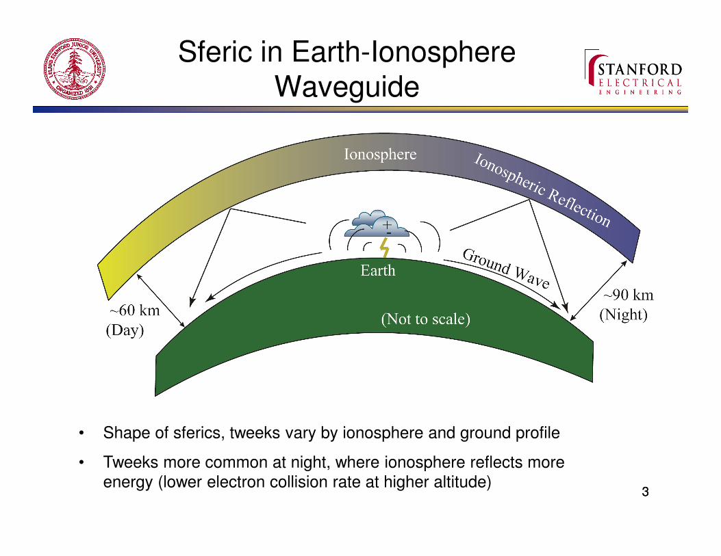
Sferic in Earth-Ionosphere Waveguide
• Shape of sferics, tweeks vary by ionosphere and ground profile
• Tweeks more common at night, where ionosphere reflects more
energy (lower electron collision rate at higher altitude)3

4
Tweek Atmospheric
Modal cutoff
Ionospheric reflections
4

5
Ray Model
• Ionosphere enables long-range propagation of emitted radio pulse
• Guided radio pulse called a “Radio Atmospheric,” or “Sferic”
• Sferic with many visible reflections forms a “Tweek Atmospheric”
• Hop arrival times related to ionospheric reflection height
• Arrive later during nighttime (higher and stronger reflection at night
than during day)
• See [Nagano 2007] for dependence of arrival time with height5

6
Modal Model
• Modal analysis: each mode dictates waveguide velocity, attenuation rate
• Discrete modes are functions of frequency, boundary reflections
• Solve by requiring phase consistency between: F1, F3
• Each mode has a cutoff frequency fc
• Below this frequency, attenuation is very high
• Nighttime ionosphere: fc ~ 1.8 kHz for the first mode (m=1)
• Based on actual ionospheric profiles, can calculate high attenuation
below 5 kHz 6

7
TE and TM Modes
• Sferic consists of a combination of TE (Transverse Electric) and
TM (Transverse Magnetic) modes
• Vertical lightning channel preferentially excites TM modes
• Horizontal loop antennas measure Hy (from TM) and Hx (from TE)
• Tweeks contain more Hx than early part of sferics
7

8
Tweek Atmospheric
• Many Ionospheric reflections visible
• Ray model: individual impulses
• Modal model: summation of modes
• Many modal cutoff frequencies visible
Modal cutoff
Ionospheric reflections
8

9
Tweek Atmospheric
1st mode cutoff
Ground Wave
Ray Hops
9
z
y
x
10
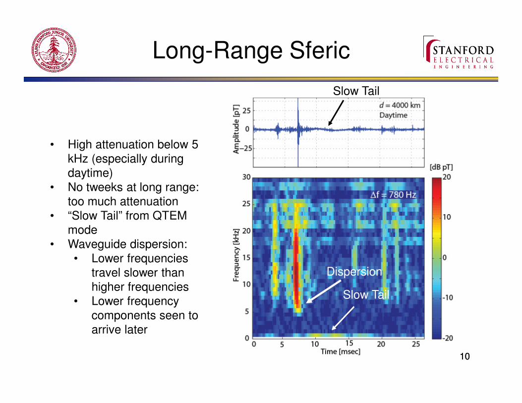
Long-Range Sferic
• High attenuation below 5
kHz (especially during
daytime)
• No tweeks at long range:
too much attenuation
• “Slow Tail” from QTEM
mode
• Waveguide dispersion:
• Lower frequencies
travel slower than
higher frequencies
• Lower frequency
components seen to
arrive later
Slow Tail
Slow Tail
Dispersion
10

11
Long-Range Sferic
• Time-domain: short impulse (top panel)
• Frequency-domain: smooth, mostly single mode (bottom panel)
• Minimum attenuation near 13 kHz 11

12
Lightning characteristics
++ +
+ +
+
+ +
+
+
+ +
+ + +
++
+
--
--
-
--
- -
---
-
++
+
+
+
++
+
Return stroke
peak current
(i.e., kA)
++ +
++
+ +
+
+
+ +
+ + +
++
-
-
--
-
++
Total charge moment
(I.e., C•km)

13
Sferic Characteristics
• VLF peak– Mostly TM Modes
– 8-12 kHz peak energy
• ELF peak– Delayed
– TEM mode
– Associated with sprites
– <1kHz energy
VLF Peak ELF “Tail”
14
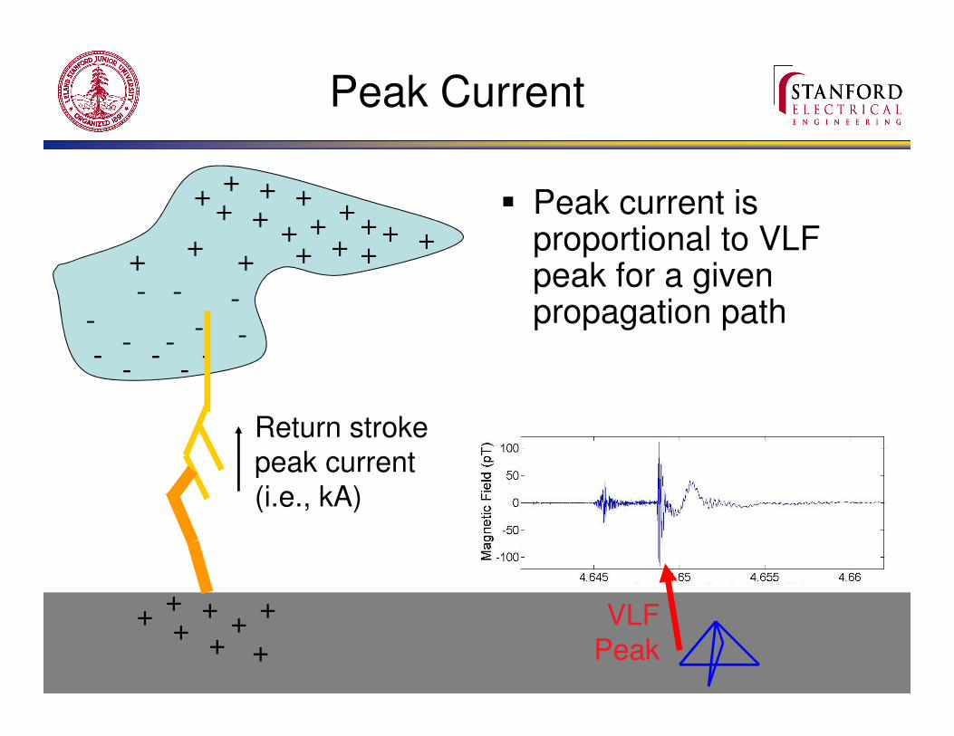
Peak Current
++ +
+ ++
+ ++
+
+ ++ + +
++
+
---
--
--- -
----
+++
+
++
+
+
Return stroke
peak current
(i.e., kA)
� Peak current is proportional to VLF peak for a given propagation path
VLF
Peak

15
Total Charge Moment
� Total ELF energy is proportional to total charge transfer
� ELF energy attenuates more in Earth-ionosphere waveguide
ELF Energy
++ +
++
+ +
+
+
+ +
+ + +
++
-
-
--
-
++
Total charge moment
(I.e., C•km)
Reising [1998]

16
Determining Azimuth
Single Frequency:
EW
NSIncident wave S
Φ
NS ~ S*cos(Φ)EW ~ S*sin(Φ)
If same constant of proportionality:
EW/NS = tan(Φ)Φ = tan-1(EW/NS)
dffEWfNS
dffEWfNSfNS
fEW
u
l
u
l
f
f
f
f
22
221
|)(||)(|
|)(||)(|)(
)(tan
+
+
≅
∫
∫−
φ
Band of frequencies: use a
weighted average
Wood and Inan [2002]

17
Determining Azimuth cont’d
0 100 200 300 400 500 600 700 800 900 1000−2000
−1000
0
1000
2000Data after band−pass filtering
NS
0 100 200 300 400 500 600 700 800 900 1000−2000
−1000
0
1000
2000
EW
milliSeconds after 17−Aug−2004 01:50:01.000 [UT]
0 2 4 6 8 10 12 14 16 18 20
0.5
1
1.5
2
x 104
A(k
)
Sferic at NotKno recorded at 17−Aug−2004 01:50:01.907 [UT]
0 2 4 6 8 10 12 14 16 18 20
30
35
40
45
50
55
60
65
frequency [kHz]
θ(k
)
θ = 55.5344, goodness measure = 1, rms = 5.3709 degrees
For each frequency, compare
magnitude from NS and EW antenna to
calculate azimuth, then average over
frequency:
Short
FFT
22
221
|)(||)(|
|)(||)(|
)(
)(tan
N
kfEW
N
kfNS
N
kfEW
N
kfNS
N
kfNS
N
kfEW
ss
f
Nf
f
Nfk
ss
f
Nf
f
Nfk
s
s
s
u
s
l
s
u
s
l
+
+
≈
∑
∑
=
=
−
φ
Calculated azimuth

18
Future Work
• Use methods in previous references to monitor ionosphere during various conditions (night/day, summer/winter, low-/mid-/high-latitude)
– As a side effect, can monitor strike locations
(especially when Tweeks are visible, see
[Nagano 2007])
18

19
References: Theoretical and Background
• Budden, K. G., “The wave-guide mode theory of wave propagation” Logos Press, 1961
– Overview of theoretical framework for waveguide propagation
• Budden, K. G. “The Propagation of Radio Waves” Cambridge University Press, 1985
– Detailed methodologies for calculating electromagnetic propagation characteristics
• Galejs, J. “Terrestrial propagation of long electromagnetic waves” Pergamon Press New York, 1972
– Calculation of earth-ionosphere waveguide propagation
• Rakov, V. A. & Uman, M. A. “Lightning - Physics and Effects” Cambridge University Press, 2003, 698
– Overview of the lightning strike, including models for electromagnetic radiation from lightning (little emphasis on waveguide propagation)
• Uman, M. A. “The Lightning Discharge” Dover Publications, Inc., 2001– Overview of lightning processes
19

20
References: Calculations
• Wait, J. R. & Spies, K. P. “Characteristics of the Earth-Ionosphere Waveguide for VLF Radio Waves” National Bureau of Standards, 1964– Numerical evaluation of waveguide propagation based on assumed
ionospheric profiles
• Nagano, I.; Yagitani, S.; Ozaki, M.; Nakamura, Y. & Miyamura, K. “Estimation of lightning location from single station observations of sferics” Electronics and Communications in Japan, 2007, 90, 22-29 – Calculation of propagation distance and ionospheric height based on
tweek measurements
• Ohya, H. et al., “Using tweek atmospherics to measure the response of the low-middle latitude D-region ionosphere to a magnetic storm,” Journal of Atmospheric and Solar-Terrestrial Physics, 2006, 697-709– Ionospheric diagnostics based on tweek measurements
20