Settle3D

Settlement and consolidation analysis

Theory Manual

© 2007-2009 Rocscience Inc.

i

Table of Contents 1 Notes ........................................................................................................................... 1 2 Stress ........................................................................................................................... 1

2.1 Effective Stress ................................................................................................... 1 2.2 Initial stress and pore pressure............................................................................ 1 2.3 Stress change due to external load ...................................................................... 3

2.3.1 Boussinesq .................................................................................................. 3 2.3.2 2:1 ............................................................................................................... 4 2.3.3 Multi-layer solution .................................................................................... 4 2.3.4 Westergaard solution .................................................................................. 5

2.4 Stress change due to change in water table elevation ......................................... 7 2.5 Stress change due to excavation ......................................................................... 7 2.6 Stress change due to rigid load ........................................................................... 7

3 Settlement ................................................................................................................... 8 3.1 Immediate settlement .......................................................................................... 8

3.1.1 Loading ....................................................................................................... 8 3.1.2 Unloading.................................................................................................... 9 3.1.3 Immediate settlement with mean stress ...................................................... 9

3.2 Settlement due to consolidation ........................................................................ 10 3.2.1 Linear ........................................................................................................ 10 3.2.2 Non-linear ................................................................................................. 10 3.2.3 Janbu ......................................................................................................... 12 3.2.4 Koppejan ................................................................................................... 14 3.2.5 Overconsolidation and underconsolidation............................................... 14

3.3 Secondary settlement ........................................................................................ 15 3.3.1 Standard method ....................................................................................... 16 3.3.2 Mesri method ............................................................................................ 17

3.4 Hydroconsolidation settlement ......................................................................... 20 4 Pore pressures ........................................................................................................... 22

4.1 Initial pore pressure........................................................................................... 22 4.2 Excess pore pressure when load is applied ....................................................... 22

4.2.1 Excess pore pressure above water table.................................................... 23 4.3 Pore pressure dissipation................................................................................... 23

4.3.1 Vertical flow ............................................................................................. 23 4.3.2 Horizontal flow due to drains ................................................................... 26 4.3.3 Horizontal and vertical flow ..................................................................... 30

4.4 Permeability and Coefficient of Consolidation................................................. 30 4.4.1 Variable permeability................................................................................ 30

4.5 Degree of consolidation .................................................................................... 31 5 Buoyancy .................................................................................................................. 33

5.1 Buoyancy effect ................................................................................................ 33 5.2 Buoyancy in Settle3D ....................................................................................... 33 5.3 Assumptions...................................................................................................... 34 5.4 Buoyancy examples .......................................................................................... 35

5.4.1 Infinite embankment, water table at the ground surface........................... 35

ii

5.4.2 Finite load, water table at depth................................................................ 36 6 Stress correction due to compaction ......................................................................... 37

6.1 Compaction effect............................................................................................. 37 6.2 Compaction Correction Examples .................................................................... 38

6.2.1 Infinite embankment, water table at the surface ....................................... 38 6.2.2 Finite load, water table at depth................................................................ 39

7 Empirical Methods.................................................................................................... 40 7.1 Schmertmann Approximation........................................................................... 40

7.1.1 Settlement calculation............................................................................... 40 7.1.2 Influence factors from Schmertmann (1970)............................................ 40 7.1.3 Modified influence factors from Schmertmann et al. (1978) ................... 41 7.1.4 Elastic modulus......................................................................................... 42

7.2 Peck, Hanson and Thornburn............................................................................ 43 7.2.1 SPT testing................................................................................................ 43 7.2.2 Settlement calculation............................................................................... 44

7.3 Schultze and Sherif ........................................................................................... 45 7.4 D'Appolonia Method......................................................................................... 47

8 References................................................................................................................. 48 9 Table of symbols....................................................................................................... 51

1

1 Notes • Directional quantities such as displacement and stress are vertical unless

otherwise noted. No subscripts are used when denoting vertical stress and vertical displacement.

• In keeping with geotechnical practice, all compressive stresses and strains are positive.

• The top of the soil horizon always has a vertical (z) coordinate of 0 and vertical coordinates below the surface are positive. Distances and displacements are positive downwards.

2 Stress

2.1 Effective Stress Settlement depends on effective stress. The effective stress is the total stress due to gravity and external loads minus the pore water pressure. The vertical effective stress, σ′ at any point is simply:

1

Where σ is the total vertical stress and u is the pore water pressure. Compressive stresses are positive.

2.2 Initial stress and pore pressure The initial total stress is just the stress due to gravity loading. At any point this stress is found by summing the weights of the above material layers. The weight of any given layer is the unit weight, γ, times the layer thickness. Therefore the initial total stress at any point is:

2

Where H is the layer thickness. The unit weight γ is set to either the saturated unit weight or the moist unit weight depending on whether the layer is below or above the piezometric line (water table). The initial pore pressure at any point is the pressure due to the weight of overlying water. If the elevation of the point of interest is z and the water table is at elevation zwt, the initial pressure is:

3

Where γwater is the unit weight of water.

u−=′ σσ

∑= Hi γσ

( ) wtwaterwti zzzzu >−= γ

wti zzu <== 0

2

The initial effective stress can then be calculated from equations 1, 2 and 3:

4

An example initial stress calculation is shown below.

4.3 m

6.0 m

γ = 16.0 kN/m3

γ = 17.8 kN/m3

γ = 18.1 kN/m3

1.2 mSand

Clay

A

At point A

σi = (1.2 m)(17.8 kN/m3) + (4.3 m – 1.2 m) (18.1 kN/m3) + (6 m)(16 kN/m3) = 173.5 kPa

ui = (4.3 m – 1.2 m)(9.8 kN/m3) + (6 m)(9.8 kN/m3) = 89.2 kPa σi′ = 173.5 kPa – 89.2 kPa = 84.3 kPa

γwater = 9.8 kN/m3

iii u−=′ σσ

3

2.3 Stress change due to external load External loads such as embankments or fills can be applied in any stage. These external loads cause a change in total stress depending on the geometry and magnitude of the external load. The stress change can be calculated by four different methods.

2.3.1 Boussinesq The Boussinesq method uses the theory of elasticity to calculate the vertical stress under a point load in a homogeneous, semi-infinite half space:

5

Where σL is the loading stress at any point and the meaning of the other symbols are as shown.

Useful solutions for stresses under different footing shapes can be obtained by integrating over the area of the footing.

Z

X Y θ z

Q

σL

θπ

σ 52 cos

23

zQ

L =

4

2.3.2 2:1 The 2:1 method assumes that the zone of influence for an applied rectangular load has a slope of 2:1 as shown. The vertical loading stress at some depth is then calculated by:

6

For a non-rectangular footing, the stress is calculated by computing the area of the load at the surface. With increasing depth, the area over which the load is applied increases at a 2:1 ratio and the magnitude of the loading stress decreases correspondingly.

2.3.3 Multi-layer solution The complete elastic solution for an arbitrary shaped foundation resting on a layered elastic medium is computed by the integration of point load solution (Green’s functions). Yue (1995, 1996) has recently provided a computational schema to efficiently compute the point load solutions through Hankel transforms. The elastic state of each homogeneous material body is governed by a set of partial differential equations and a set of boundary conditions. In this case of homogeneous elastic layers the boundary conditions are the set of matching stress and displacement conditions. Hankel transformation is used to convert the set of partial differential equations governing each material layer to a set of ordinary differential equations and the respective boundary conditions to algebraic expressions. Yue (1995, 1996) solved the systems of ordinary differential equations with the matching boundary conditions to a set of algebraic system of equations, unknowns being specially constructed functions in the Hankel transform domain. The stresses and displacements can be obtained through combinations of the

Q

2 1

BL

σL

z

( )( )zLzBQ

L ++=σ

5

inverse transforms of these functions. Due to extreme complexity of the functions in the Hankel transform domain, we need to resort to numerical methods which are computationally intensive and therefore very slow. For our purpose, we need to perform two levels of numerical integration: the first level of computation evaluates the point load solutions, and the subsequent level of computation performs numerical quadrature to evaluate stresses and displacements due to the distributed loading over the given area. We have developed an extremely efficient computational method by combining the two computational levels in different order. We have also enhanced the numerical accuracy by converting the area integrals into boundary integrals by a method developed by Vijayakumar, Yacoub and Curran (2000). This boundary conversion method also circumvents the numerical difficulty associated with the singularity of the point load solutions. For any rapidly varying stress locations such as in the vicinity of boundaries, a form of adaptive special subdivision scheme is used.

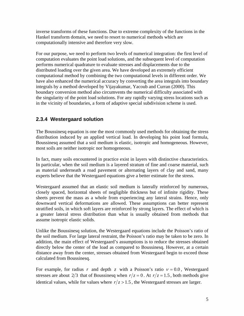
2.3.4 Westergaard solution The Boussinesq equation is one the most commonly used methods for obtaining the stress distribution induced by an applied vertical load. In developing his point load formula, Boussinesq assumed that a soil medium is elastic, isotropic and homogeneous. However, most soils are neither isotropic nor homogeneous. In fact, many soils encountered in practice exist in layers with distinctive characteristics. In particular, when the soil medium is a layered stratum of fine and coarse material, such as material underneath a road pavement or alternating layers of clay and sand, many experts believe that the Westergaard equations give a better estimate for the stress. Westergaard assumed that an elastic soil medium is laterally reinforced by numerous, closely spaced, horizontal sheets of negligible thickness but of infinite rigidity. These sheets prevent the mass as a whole from experiencing any lateral strains. Hence, only downward vertical deformations are allowed. These assumptions can better represent stratified soils, in which soft layers are reinforced by strong layers. The effect of which is a greater lateral stress distribution than what is usually obtained from methods that assume isotropic elastic solids. Unlike the Boussinesq solution, the Westergaard equations include the Poisson’s ratio of the soil medium. For large lateral restraint, the Poisson’s ratio may be taken to be zero. In addition, the main effect of Westergaard’s assumptions is to reduce the stresses obtained directly below the center of the load as compared to Boussinesq. However, at a certain distance away from the center, stresses obtained from Westergaard begin to exceed those calculated from Boussinesq. For example, for radius r and depth z with a Poisson’s ratio 0.0=ν , Westergaard stresses are about 32 that of Boussinesq when 0=zr . At 5.1=zr , both methods give identical values, while for values where 5.1>zr , the Westergaard stresses are larger.

6

Similar to Boussinesq, closed form expressions for the stress profiles of: 1) the center of a uniformly loaded circular area and 2) the corner of a uniformly loaded rectangular area are both available. Further, the contributions of adjacent loads can be superimposed to give the total stress at a given point. In general, sedimentary soils like natural clay strata accentuate the non-isotropic condition of the soil medium. Hence, for these cases, the Westergaard equations serve as better models for reality. However, practicing geotechnical engineers often prefer Boussinesq primarily because this method gives more conservative results. In any case, the choice of analysis depends on how closely field conditions match a model’s basic assumptions. As described in Venkatramaiah (2006), for a soil medium with Poisson’s ratio ν , the vertical stress zσ due to a point load Q as obtained by Westergaard is given by:

322 2

1 1 22 2 2

1 22 2

zQz r

z

νπ νσνν

−−=

⎡ ⎤−⎛ ⎞ ⎛ ⎞+⎢ ⎥⎜ ⎟ ⎜ ⎟−⎝ ⎠ ⎝ ⎠⎢ ⎥⎣ ⎦

7

For large lateral restraint, ν may be taken as zero. The vertical stress below the center of a circular footing can be obtained analytically by integrating equation 7. The solution of which is given by:

⎥⎥⎥⎥

⎦

⎤

⎢⎢⎢⎢

⎣

⎡

⎟⎠⎞⎜

⎝⎛+

−=2

1

11

za

qz

η

σ 8

where: ννη

2221

−−

= and

q is a uniform load. The vertical stress below the corner of a rectangular footing can be obtained analytically by integrating equation 7. The solution of which is given by:

⎟⎠⎞

⎜⎝⎛

⎟⎠⎞

⎜⎝⎛

−−

+⎟⎠⎞

⎜⎝⎛ +⎟

⎠⎞

⎜⎝⎛

−−

= −22

2

221 1

222111

2221cot

2 nmnmq

z νν

νν

πσ 9

where: zLm /= zWn /=

7

L and W are the respective lengths and widths of the rectangle z is the depth and q is a uniform load. For the case of a square, L = B. Hence, m = n.

2.4 Stress change due to change in water table elevation If the water table is lowered, then some soil will change from being saturated to unsaturated. This change in weight will cause a decrease in the total stress at all points below the original water table elevation. However, the water table drop will also cause a decrease in pore pressures, and therefore the effective stress will increase by equation 1. This effect is generally larger than the change in total stress; therefore there is generally a net increase in effective stress. The opposite will occur for a water table rise.

2.5 Stress change due to excavation When material is excavated, the weight of excavated material is calculated from the unit weight and this is applied as an upward stress at the bottom of the excavation. The stress at any point below this is then calculated as if a stress was applied due to a negative load (section 2.3). There is no attempt to calculate true three-dimensional stress changes due to excavations. Also, no changes in water pressure are considered.

2.6 Stress change due to rigid load We use a point load based (Green’s function) error minimization hybrid method for the computation of the stresses resulting from a loaded rigid foundation. The rigid elastic foundation problem is one of the important modeling problems in Civil Engineering practice. The entire displacement of a rigid foundation will follow a linear function with only 3 hitherto unknown variables. On the other hand, the traction on the elastic body will follow an unknown, but much more complicated functionality. The coupling between the rigid body and the elastic body lying below is done by minimizing the average of the square (RMS) of the difference between the displacements. Here, a method using linear piece-wise functions with several parameters via triangular discretizations is adopted (Vijayakumar et al, 2009). The elastic response of the piece-wise functions (with the unknown parameters) is calculated by the integration of point load solutions over the triangular discretizations. The point load solutions are available in the analytical form for a homogeneous elastic body and via numerically using the method outlined in Yue (1995, 1996) for a layered elastic body. The unknown parameters governing the linear functional form in each triangulation are calculated by the overall minimization of the RMS error as mentioned above. Once the parameters are known, the stress and displacement at any point in the elastic body can be calculated using the boundary quadrature method outlined in Vijayakumar et al, (2000). By performing several numerical tests, it has been found that the error minimization method is a very efficient and accurate method for the rigid foundation problem.

8

3 Settlement The total settlement is the sum of three components:

• Immediate or initial settlement • Settlement due to consolidation • Secondary settlement (creep)

Each of these is calculated as follows.

3.1 Immediate settlement

3.1.1 Loading The immediate settlement occurs instantly after load is applied and is assumed to be linear elastic. The strain for each element in a string can then be easily calculated from the 1D modulus and the effective stress. The 1D modulus (or constrained modulus) (Es) is input directly into Settle3D. The relationship between the 1D modulus and 3D Young’s modulus (E) is:

10

Where ν is the Poisson’s Ratio. The vertical strain in each sublayer is calculated by:

11

Where σΔ is the change in vertical total stress. Initial settlement is then calculated from these strains. For each string, the bottom point is assumed to be fixed (non-moving). The vertical displacement of the point second from bottom is then:

12

Where h is the original thickness of the bottom sublayer. The settlement of the ith point is then the settlement of the point below (i+1) plus the settlement in sublayer i:

13

( )( )ν

νν−

−+=

1211

sEE

sEσε Δ

=

hz εδ =Δ=

iiii hεδδ += +1

9

3.1.2 Unloading In Settle3D, the user may supply an unload/reload modulus. If unloading occurs (due to decreasing the magnitude of an existing load, or adding an excavation) then the unload/reload modulus (Esur) is used in place of Es in equation 11. If the soil is then reloaded, Esur continues to be used until the soil sublayer reaches its previous stress state, at which time Es is again used in equation 11 to compute strain as shown.

3.1.3 Immediate settlement with mean stress By default, settlement is calculated using only the vertical stress. A more accurate analysis can be performed by using the three-dimensional mean stress in the calculations. The mean stress at any point is the average of the volumetric stress components:

14

γ

σ

Loading Slope = Es Unload/reload

Slope = Esur

h1

h2

h3 δ3 = ε3h3

δ2 = δ3 + ε2h2

δ1 = δ2 + ε1h1

( ) ( )32131

31 σσσσσσσσ ++=++= MzzyyxxM or

10

The Immediate Settlement is then calculated by computing the strain in each sublayer:

15

Where ν is the Poisson’s Ratio, σΔ is the change in total vertical stress, MσΔ is the change in mean stress and E is the Young’s modulus. When mean stress is being used, Young's modulus is input directly for each material (not the 1D modulus). The unload/reload modulus Eur may be used in place of E as described above. The mean stress is not used in the calculation of Consolidation Settlement and Secondary Settlement because the relationship between strain and mean stress is not clearly defined for non-linear materials.

3.2 Settlement due to consolidation Settlement due to consolidation progresses gradually as pore pressures dissipate and effective stresses increase. The settlements are calculated from the strains in each sublayer as in equation 13, however the calculation of the strains depends on the type of material as follows.

3.2.1 Linear Linear material is assumed to be linear elastic. Therefore the change in vertical strain for any given element for a change in vertical effective stress Δσ′ is simply:

16

Where mv is the one-dimensional compressibility. During unload/reload cycles, mv is replaced with the unload/reload compressibility mvur.

3.2.2 Non-linear In non-linear material, the modulus is not constant but is a function of stress. This relationship is most commonly shown on a graph of void ratio versus the logarithm of effective stress as shown.

( ) ( ) ( )1 3 M

Eν σ ν σ

ε+ Δ − Δ

=

σε ′Δ=Δ vm

11

1.6

1.7

1.8

1.9

2

2.1

2.2

10 100 1000Vertical effective stress (kPa)

Void

Rat

io

Recompression curveSlope = C r

Virgin curveSlope = C c

P c

Unload-reload curveSlope = C r

The void ratio in a soil is the ratio of the volume of voids to the volume of solids

17

The stress level Pc is the preconsolidation stress and represents the maximum effective stress experienced by the soil in the past. If a soil is experiencing an effective stress less than Pc it is overconsolidated. The relationship between the void ratio and the logarithm of the effective stress is given by the recompression index, Cr. A soil that has a stress greater than or equal to Pc is normally consolidated and its deformation is dictated by the compression index Cc. A soil that is unloading is always considered overconsolidated as shown. For a stress change in an overconsolidated soil layer, the change in void ratio, Δe, can be calculated from the initial effective stress, σi′ and the final effective stress, σf′ by:

18

Vertical strain is related to void ratio by:

s

v

VVe =

⎟⎟

⎠

⎞

⎜⎜

⎝

⎛

′

′−=Δ

i

frCe

σ

σlog

12

19

Where e0 is the initial void ratio. Therefore,

20

For a normally consolidated soil, the equation is the same with Cr replaced with Cc. It is also possible for a soil layer to start out overconsolidated and end up normally consolidated if the final stress is greater than Pc. In this case, the vertical strain can be calculated by:

21

Note that the initial stress does not necessarily have to refer to the initial in-situ stress due to gravitational loading. For a multi-stage analysis, the change in strain is computed for each stage by using the effective stress at the start of the stage and the effective stress at the end of the stage in equation 20 or 21. Strains may also be calculated using strain based versions of the compression indices, Ccε and Crε. In this case, stress is related directly to strain, rather than void ratio so for a completely overconsolidated material equation 20 becomes:

Equations involving normally consolidated material are formed similarly.

3.2.3 Janbu The Janbu approach (Janbu, 1963, 1965) can be linear or non-linear depending on the stress exponent, a. The 1D modulus, M is given by:

22

01 ee

+Δ

−=ε

⎟⎟

⎠

⎞

⎜⎜

⎝

⎛

′

′

+=Δ

i

fr

eC

σ

σε log

1 0

⎟⎟

⎠

⎞

⎜⎜

⎝

⎛ ′

++

⎟⎟

⎠

⎞

⎜⎜

⎝

⎛′+

=Δc

fc

i

cr

PeCP

eC σ

σε log

1log

1 00

⎟⎟

⎠

⎞

⎜⎜

⎝

⎛

′

′=Δ

i

frC

σ

σε ε log

a

r

rmM−

⎟⎟

⎠

⎞

⎜⎜

⎝

⎛′′′=

∂∂

=

1

σ

σσεσ

13

Where m is a modulus number and rσ ′ is a reference stress, usually equal to 100 kPa. The change in strain for any given change in stress is then found by integrating equation 22. This yields: For a > 0

23

For a = 0

24

Where σi′ and σf′ are the initial and final effective stress for the calculation stage. For a = 1, the Janbu method is the same as the linear method with

1

v r

mm σ

=′

a = 1

When a = 0, the Janbu method is the same as the non-linear method with

01ln10c

emC+

= a = 0

These equations are written for normally consolidated soil. For overconsolidated soils, m can be replaced by mr, the recompression modulus number. Alternatively, the user can specify a constant modulus Moc for overconsolidated soil. If this option is chosen, then:

25

and

26

⎥⎥⎥

⎦

⎤

⎢⎢⎢

⎣

⎡

⎟⎟

⎠

⎞

⎜⎜

⎝

⎛′

′−⎟

⎟

⎠

⎞

⎜⎜

⎝

⎛

′

′=Δ

a

r

i

a

r

f

ma σ

σ

σ

σε 1

′

′=Δ

i

f

m σ

σε ln1

ocMM =

⎟⎠⎞⎜

⎝⎛ ′−′=Δ if

ocMσσε 1

14

3.2.4 Koppejan The Koppejan method (Koppejan, 1948) computes strain with the following equation:

27

Where U is the degree of consolidation, Cp and Cs are compression constants, t is time, σi′ is the initial effective stress and σf′ is the final effective vertical stress after loading and consolidation. The degree of consolidation U is computed for any location at any time by:

28

Where ue is the excess pore water pressure and σ′ is the effective stress. For overconsolidated material, Cp and Cs are replaced by Cp′ and Cs′. In Settle3D, an incremental version is used to get the change in strain for any time step, Δt:

29

For the first time step, when t equals 0, the logarithm is replaced by log(Δt). This equation allows the settlement to be calculated at intermediate times during a settlement analysis. The problem with the Koppejan method is how to deal with changing loads. Traditionally, some type of superposition is used (see van Baars, 2003). Since Settle3D computes the strain in an incremental fashion, this is not really necessary. Instead, Settle3D performs the following steps when a change in loading occurs:

• The current effective vertical stress is recorded and used as σi′ in subsequent time steps.

• The degree of consolidation is calculated using the new σi′.

3.2.5 Overconsolidation and underconsolidation The Non-linear and Janbu methods use the preconsolidation stress, Pc, to determine if the soil is over-consolidated or normally consolidated. Instead of specifying Pc you may specify either the overconsolidation ratio (OCR) or overconsolidation margin (OCM). The OCR is related to Pc by

( ) ⎟⎟

⎠

⎞

⎜⎜

⎝

⎛

′

′

⎟⎟⎠

⎞⎜⎜⎝

⎛+=

i

f

sp

tCC

U

σ

σε lnlog1

′−′+−=

ie

e

u

uUσσ

1

⎟⎟

⎠

⎞

⎜⎜

⎝

⎛

′

′

⎟⎟⎠

⎞⎜⎜⎝

⎛⎟⎠⎞

⎜⎝⎛ Δ+

+Δ

=Δi

f

sp ttt

CCU

σ

σε lnlog1

15

30

Where σ′ is the current effective stress. The OCM is related to Pc by

31

(Coduto, 1999, p391). Therefore if OCR = 1 or OCM = 0 and there is no load applied, then the material is all normally consolidated and each point in the soil has a Pc equal to the in-situ stress due to gravity. When a load is applied, the material remains normally consolidated and Pc increases with stress. If OCR > 1 or OCM > 0 then the material is all overconsolidated and at each point in the soil, Pc equals OCR times the in-situ stress, or OCM plus the in-situ stress. If a load is then applied, the material remains overconsolidated and Pc remains constant until the stress in the soil surpasses Pc at which point the material becomes normally consolidated and Pc increases as stress increases. If the material is then unloaded, it will then become overconsolidated again and Pc will remain constant and equal to the highest stress attained by the soil. If OCR is less than 1 or if OCM is negative, then the soil is underconsolidated. This means that there is still excess pore pressure in the soil due to a previous load that has not yet dissipated. To account for this, Settle3D adds an excess pore pressure to all points in the soil such that

32

or

33

Where σi′ is the initial (in-situ) effective stress due to gravity. Pc is then set according to equation 30 or equation 31 and the material behaves as if it is normally consolidated (i.e. Cc is used to compute displacements in the non-linear model). As the excess pore pressure dissipates, Pc increases as the effective stress increases. Note that a material can only be underconsolidated if the ‘Time-dependent Consolidation Analysis’ option is turned on in the Project Settings.

3.3 Secondary settlement Secondary settlement, or creep, can occur at a constant effective stress for some types of soils. There are several different methods for computing the magnitude of secondary

σ ′= cPOCR

( ) ′−= ie OCRu σ1

σ ′−= cPOCM

OCMue −=

16

settlement – especially when a surcharge load is applied. Settle3D implements two different methods as described in the subsequent sections.

3.3.1 Standard method The magnitude of the secondary settlement is assumed to vary linearly with the logarithm of time as shown below.

2.25

2.3

2.35

2.4

2.45

2.5

2.55

2.6

2.65

0.1 1 10 100 1000 10000

Time

Voi

d ra

tio

Secondary compressionSlope = Cα

tp

e p

Using the void ratio at the end of primary consolidation, ep, the change in secondary vertical strain for a change in time from t1 to t2 is

34

The secondary displacement can then be calculated by multiplying by the layer thickness as in equations 12 and 13. For linear and Janbu materials, there is no void ratio associated with them. Therefore instead of Cα, the user must input the modified secondary compression index or strain based secondary compression index

35

1

2log1 t

te

C

pS +

=Δ αε

peCC+

=1

ααε

17

So that equation 34 becomes:

1

2logttCS αεε =Δ

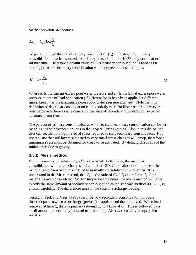
To get the time at the end of primary consolidation (tp) some degree of primary consolidation must be assumed. A primary consolidation of 100% only occurs after infinite time. Therefore a default value of 95% primary consolidation is used as the starting point for secondary consolidation where degree of consolidation is

36

Where ue is the current excess pore water pressure and ue0 is the initial excess pore water pressure at time of load application (if different loads have been applied at different times, then ue0 is the maximum excess pore water pressure attained). Note that this definition of degree of consolidation is only strictly valid for linear material however it is only being used here as an estimate for the start of secondary consolidation, so perfect accuracy is not crucial. The percent of primary consolidation at which to start secondary consolidation can be set by going to the Advanced options in the Project Settings dialog. Also in this dialog, the user can set the minimum level of stress required to start secondary consolidation. It is not realistic that soil layers subjected to very small stress changes will creep, therefore a minimum stress must be obtained for creep to be activated. By default, this is 1% of the initial stress due to gravity.

3.3.2 Mesri method With this method, a value of C∝ / Cc is specified. In this way, the secondary consolidation will reflect changes in Cc. In Settle3D, Cc remains constant, unless the material goes from overconsolidated to normally consolidated or vice versa. It is understood in the Mesri method, that Cc in the ratio of C∝ / Cc can refer to Cr if the material is overconsolidated. So, for simple loading cases, the Mesri method will give exactly the same amount of secondary consolidation as the standard method if C∝ / Cc is chosen carefully. The differences arise in the case of surcharge loading. Terzaghi, Peck and Mesri (1996) describe how secondary consolidation follows a different pattern when a surcharge (preload) is applied and then removed. When load is removed at time ts, there is primary rebound up to a time of tpr. This is followed by a small amount of secondary rebound to a time of tl. After tl, secondary compression restarts.

0

1e

e

uuU −=

18

Settlement versus time for a surcharge load, from Terzaghi et al., 1996 The postsurcharge secondary compression index, C∝′ is not constant with time, as shown in the above figure. It generally starts small and then increases in magnitude. To make secondary settlement calculations easier, a secant index, C∝″ is proposed as shown. The secondary compression at any time t after tl can then be calculated from C∝″. The method of calculating secondary compression for a surcharge load proceeds as follows: A surcharge is applied. Consolidation occurs and the maximum effective vertical stress before the surcharge removal is σvs′. The surcharge is removed, leaving behind the desired final load. Rebound occurs and the effective vertical stress at the end of primary rebound is σvf′. The effective surcharge ratio is then calculated:

37

The value for Rs′ is then used to compute the time to the start of secondary compression tl by:

38

Both tl and tpr are measured relative to the time of load removal, ts. These equations are obtained from laboratory studies as described in Terzaghi et al. (1996), Mesri et al. (1997) and Mesri et al. (2001). It is assumed that no secondary settlement occurs until time tl (the secondary rebound is ignored). To calculate the secondary settlement at any time t after tl, the ratio of C∝″/C∝ is determined from one of the following charts, depending on the material type. Charts are obtained from Terzaghi et al. (1996), Mesri et al. (1997) and Mesri et al. (2001).

( )/ 1s vs vfR σ σ′ ′ ′= −

PeatRtt

claysSoftRtt

sprl

sprl

′=

⎟⎠⎞⎜

⎝⎛ ′=

10

1007.1

19

With the Mesri method, a value of C∝ / Cc is generally specified. Therefore the secondary strain at time t is:

39

lcp

cS t

tCC

CC

eC log

1 α

ααε″

+=Δ

Middleton Peat

20

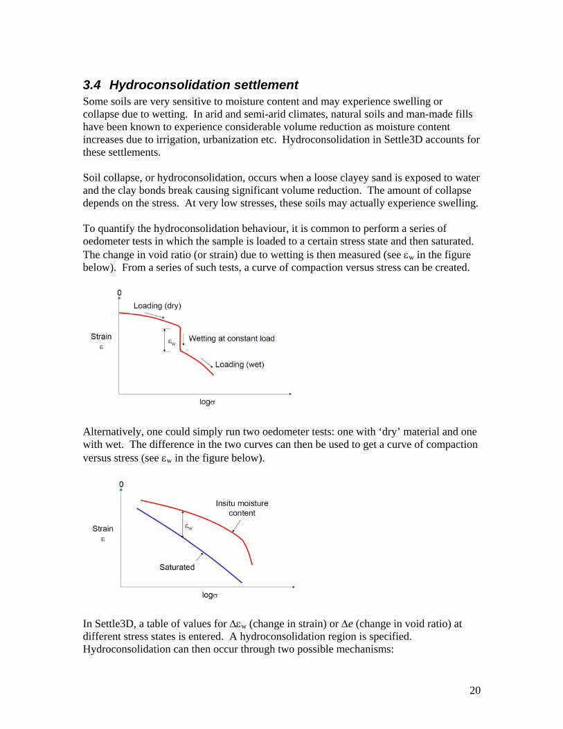
3.4 Hydroconsolidation settlement Some soils are very sensitive to moisture content and may experience swelling or collapse due to wetting. In arid and semi-arid climates, natural soils and man-made fills have been known to experience considerable volume reduction as moisture content increases due to irrigation, urbanization etc. Hydroconsolidation in Settle3D accounts for these settlements. Soil collapse, or hydroconsolidation, occurs when a loose clayey sand is exposed to water and the clay bonds break causing significant volume reduction. The amount of collapse depends on the stress. At very low stresses, these soils may actually experience swelling. To quantify the hydroconsolidation behaviour, it is common to perform a series of oedometer tests in which the sample is loaded to a certain stress state and then saturated. The change in void ratio (or strain) due to wetting is then measured (see εw in the figure below). From a series of such tests, a curve of compaction versus stress can be created.

Alternatively, one could simply run two oedometer tests: one with ‘dry’ material and one with wet. The difference in the two curves can then be used to get a curve of compaction versus stress (see εw in the figure below).

In Settle3D, a table of values for Δεw (change in strain) or Δe (change in void ratio) at different stress states is entered. A hydroconsolidation region is specified. Hydroconsolidation can then occur through two possible mechanisms:

21

1. The water table is raised. When this happens, the soil will collapse if it is within the hydroconsolidation region that was previously dry, and then becomes wet. Note that soil that is below the water table in Stage 1 is assumed to be collapsed already and will not collapse further.

2. A wetting stage can be specified. This might simulate a broken water pipe or some other wetting mechanism that does not necessarily raise the water table. At this stage and within the specified region, the soil will collapse.

The collapse in the soil is calculated by first calculating the stress at the centre of each sublayer in the collapsing region. From this stress, the change in strain is determined and applied according to the user-defined strain versus stress relationship. Therefore an instant collapse (or swelling) is observed. By default, Settle3D assumes unsaturated unit weight for a wetted material above the water table. However you can force the program to consider the saturated unit weight by checking the appropriate box in the hydroconsolidation material parameters dialog. If this option is chosen, the saturated unit weight is only used in calculating the hydroconsolidation settlement. It will not change the stresses plotted in graphs and contour plots and it will not affect calculation of other settlements (immediate, consolidation or secondary).

22

4 Pore pressures

4.1 Initial pore pressure The initial pore pressure at any point is the pressure due to the weight of overlying water as given in equation 3.

4.2 Excess pore pressure when load is applied By default, when a load is applied, the pore pressure at each node increases by an amount equal to the change in vertical stress at that node:

40

The excess pore pressure is then simply the pore pressure minus the initial pore pressure due to gravity:

41

A more accurate approach is to set the change in pore pressure equal to the change in undrained mean stress. This can be accomplished by choosing the Use mean 3D stress option in the Project Settings (Advanced). The undrained mean stress is the average of the volumetric stress components for an undrained (incompressible) material:

42

An undrained material has a Poisson’s ratio ν = 0.5. Setting the initial pore pressure equal to the initial stress is only strictly true for a fluid of infinite stiffness in a fully saturated soil. For partially saturated material, the pore spaces are partly filled with air. In this case the pore fluid (air + water) cannot be considered infinitely stiff. Therefore some load is initially carried by the soil matrix. To account for this effect, the user can specify the Skempton pore pressure coefficient B such that

43

(Skempton, 1954). The coefficient B ranges from 0 for dry soil to 1 for fully saturated soil. If only vertical stresses are being used, then the parameter B is set such that

44

By default in Settle3D, B or B = 1.

σΔ=Δu

( ) ( ) 5.03215.0 31

31

==++=++= νν

σσσσσσσσ undrainedMzzyyxx

undrainedM or

ie uuu −=

( )undrainedMBu σΔ=Δ

( )σΔ=Δ Bu

23

4.2.1 Excess pore pressure above water table By default, the soil is assumed to be dry above the water table, so an applied load does not generate excess pore pressure above the water table. If you want the soil to behave as if it were saturated above the water table, then you can select the Generate excess pore pressures above water table checkbox under the Groundwater tab of the Project Settings dialog. In this case, applied loads will generate excess pore pressure above the water table, as if the material were saturated with B = 1.

4.3 Pore pressure dissipation

4.3.1 Vertical flow Vertical consolidation is dictated by Terzaghi’s 1D consolidation equation:

45

Where ue is the excess pore pressure, cv is the coefficient of consolidation and z is the vertical distance below the ground surface. The excess pressure at any time is calculated from this equation and is then used to calculate the effective stress (equation 1). Strains can then be calculated depending on the material type and the strains are used to calculate settlement (equations 12 and 13). This equation can be solved analytically for a single layer with linear stiffness. For multiple layers with differing coefficients of consolidation and different thicknesses, a finite difference approach can be used to solve for the pore pressure. This is the approach adopted by Settle3D. If the problem domain is discretized in time and space as shown below, equation 45 can be replaced by:

tuu

tu titti

Δ−

=∂∂ Δ+ ,,

46

( )( )

[ ]( )

[ ]⎭⎬⎫

⎩⎨⎧

+−Δ

+⎭⎬⎫

⎩⎨⎧

+−Δ

−=∂∂

Δ++Δ+Δ+−+− ttittittiv

tititiv

v uuuh

cuuuh

cxuc ,1,,12,1,,122

2

221 φφ

Where φ is a time weighting parameter. In Settle3D, φ = 0.5. Note that we have dropped the subscript, e, that indicates excess pore pressure. These equations still refer to excess pore pressure but the subscript has been dropped to simplify the notation.

2

2

zuc

tu e

v ∂∂

=∂∂

24

Explicit solution This equation can then be solved implicitly or explicitly. The explicit solution calculates the pressure at time t+Δt for each node sequentially. Initial excess pore pressures at time t are calculated for all nodes according to equation 43 or 44. The pore pressure at time t+Δt for node i is then calculated by rearranging equation 46 to give:

( )( )

( ) ( ) tiv

vvttittititi

v

vtitti u

tchtc

htcuuuu

tchtcuu ,22,1,1,1,12,, 1

21

⎥⎦

⎤⎢⎣

⎡

Δ+ΔΔ

−Δ

Δ+++++

Δ+ΔΔ

+= Δ++Δ+−+−Δ+

Note that the solution for pressure at node i depends on the pressure at node i+1, which has not yet been calculated, so the solution requires iterations. In addition, the timestep, Δt, must be small to ensure stability:

( )vcht

2Δ<Δ β explicit

Where β is a dimensionless factor that must be less than 0.5. For accurate results, β is set to 0.2 in Settle3D.

Δt

ui,t ui,t+Δt

ui-1,t

ui+1,t

hi-1

hi

z

time

25

Implicit solution For models with long time scales, the explicit solution can be slow, therefore an implicit solution is also implemented in Settle3D. To perform the implicit analysis, equation 46 is rearranged such that all the pressures at time t+Δt are on the left hand side:

( ) ( )titi

vtittitti

vtti uu

tchuuu

tchu ,1,

2

,1,1,

2

,12222 +−Δ++Δ+Δ+− −⎟⎟

⎠

⎞⎜⎜⎝

⎛Δ

Δ−+−=+⎟⎟

⎠

⎞⎜⎜⎝

⎛Δ

Δ+−

One equation of this form is written for each node. This leads to a system of linear algebraic equations that can be solved simultaneously using matrix inversion. The system is unconditionally stable, regardless of Δt, however results are poor if Δt is too low:

( )vcht

2

31 Δ

>Δ implicit

(Abid and Pyrah, 1988) Choice of solution method In Settle3D, explicit timesteps are executed until the time is greater than the minimum timestep required for the implicit approach. The solution then switches to the implicit approach for the remainder of the solution. As the implicit solution progresses, the timestep is gradually increased. This speeds up the solution without loss of accuracy because of decreasing pore pressure gradients. Non-uniform material Most models will not have a constant value for Δh or cv since different material layers will be present. To account for this, the equations are adjusted slightly. All ui+1 terms are multiplied by a factor αi:

i

i

i

ii h

hkk 1

1

−

−

=α

Where ki-1 , ki are the permeabilities of the sublayers above and below the node, hi-1 , hi are the thicknesses of the sublayers above and below the node. All ui terms are split into two pieces so for example, in the implicit solution, the term for ui,t+Δt becomes:

( ) ( )( )

( )( ) tti

iv

i

ivitti

v

utc

htc

hutc

hΔ+

+

+Δ+ ⎟⎟

⎠

⎞⎜⎜⎝

⎛Δ

Δ+

ΔΔ

++→⎟⎟⎠

⎞⎜⎜⎝

⎛Δ

Δ+ ,

1

21

2

,

2

122 α

26

Boundary conditions Nodes on the boundaries can be drained or undrained. For a drained boundary, the pressure is set to 0 and the calculations are not performed at this node. An undrained node on the boundary is assumed to be impermeable. To account for this, a dummy node is generated to permit the finite difference calculation to proceed. For example, if the bottom node is impermeable, then a dummy node is created below the bottom node. The distance between the bottom node and the dummy node is the same as the distance between the bottom node and the node second from bottom. The pressure on the dummy node is assigned a pressure equal to the pressure of the node second from bottom. In this way, there will be no flow across the bottom node.

4.3.2 Horizontal flow due to drains Drains may be added to speed consolidation by permitting horizontal flow. If an array of drains is constructed, then the distance the water must flow to the nearest drain is short and the pore pressure dissipation will be greatly accelerated. In addition, the horizontal permeability is often greater than the vertical permeability so horizontal flow is faster than vertical flow. In general, an array of drains is constructed in a square or triangular pattern.

Soil

Δh

Δh Impermeable boundary

un-1

un

un-1

Dummy node

27

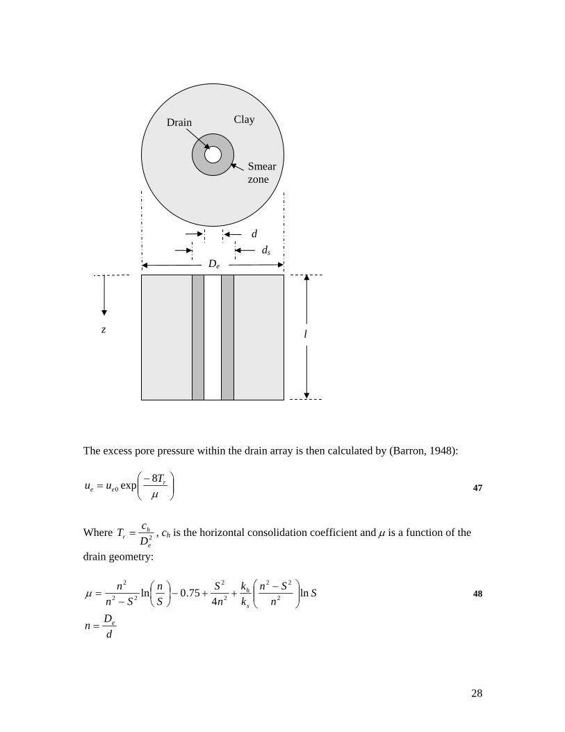
These drain patterns ensure that the entire area within the grid is being drained. Each drain therefore has associated with it a zone of influence. It is assumed that horizontal flow occurs only toward the drain within this zone of influence, i.e. the edge of each zone of influence is an impermeable boundary. For a triangular array, the zone of influence is hexagonal and for a square array, the zone is square. To simplify the mathematics, each zone of influence is assumed to be circular and the diameter of the equivalent circle is calculated as follows: De = 1.05D Square pattern De = 1.13D Triangular pattern Where D is the actual spacing between the drains as shown. For each drain, the pore pressure at any given point in the zone of influence at any given time can be calculated analytically using the radial flow equation. The average pore pressure within the zone of influence can then be calculated at any time. This average value will be the same for all drains, therefore everywhere within the drain array is assumed to have the same pore pressure at any given time. To make the equations more realistic, a smear zone can be included. When a drain is constructed, the soil close to the drain walls is disturbed forming a smear zone. The permeability in the smear zone may be lower than the permeability of the undisturbed soil and this will affect the pore pressure dissipation. The geometry of the problem for a single drain is shown below:

De

Square pattern

drain

Triangular pattern

D

De

D

28

The excess pore pressure within the drain array is then calculated by (Barron, 1948):

47

Where 2e

hr D

cT = , ch is the horizontal consolidation coefficient and μ is a function of the

drain geometry:

48

dDn e=

z

d

ds

De

Clay

Smear zone

Drain

l

⎟⎟⎠

⎞⎜⎜⎝

⎛ −=

μr

eeTuu 8exp0

Sn

Snkk

nS

Sn

Snn

s

h ln4

75.0ln 2

22

2

2

22

2

⎟⎟⎠

⎞⎜⎜⎝

⎛ −++−⎟

⎠⎞

⎜⎝⎛

−=μ

29

ddS s=

And h

s

kk

is the ratio of horizontal permeability in the undisturbed zone to permeability in

the smear zone. A common value of S is about 1.5–3 (Hansbo, 1979). If S = 1 and h

s

kk

=

1, then there is no smear zone. Equivalent diameter of band shaped drains Wick drains are generally not cylindrical as assumed in the above equations. Kjellman (1948) showed that the draining effect of a drain depends on the circumference of its cross section and not on the cross-sectional area. Therefore the equivalent diameter of a band shaped drain with width b and thickness t is

49

Well resistance The above equations assume that the drain itself has an infinite permeability. In fact this is not the case and for long drains, the well resistance may slow down fluid flow. To account for this, μ in equation 47 should be replaced by μr (Hansbo, 1981)

( )2 /r h wz l z k qμ μ π= + − Where l is the length of the well, z is the distance from the top of the well, kh is the horizontal permeability of the clay and qw is the discharge capacity of the well (volume / time). If the well drains at both the top and the bottom (i.e. the bottom intersects a highly permeable layer), the l is set to half the length of the drain. A Note on permeability Although equation 47 uses ch to compute the pore pressure decrease due to drains, most practitioners will likely not have this information. In Settle3D, the user may choose to enter the permeability, kh instead. The value for ch will then be calculated from the vertical stiffness (see section 4.4). This is not strictly correct since the horizontal stiffness should be used in the calculation, however it is thought that the error introduced with this method will be small compared to the uncertainty in the input permeability.

( )π

tbd +=

2

30

4.3.3 Horizontal and vertical flow The pore pressure at any time is a function of pressure loss due to vertical drainage and pressure loss due to horizontal flow into drains. To compute the total pore pressure at each time step, the pressure due to vertical flow is calculated first using the finite difference approach in equation 46. This pressure is then used as the starting pressure for the calculation of equation 47 that accounts for pressure loss due to vertical drains. The result of equation 47 is then the ultimate pressure for the timestep.

4.4 Permeability and Coefficient of Consolidation To solve for pore pressures in a multi-layered material, both the material permeability (k) and material coefficient of consolidation (cv) are required. However in Settle3D, the user only needs to specify one or the other of these quantities. This is because these quantities are not independent and are related to each other through the material stiffness. The material stiffness depends on the material type. Therefore if the user enters cv, permeabilities are calculated as follows:

wvvmck γ= linear material

( ) ′+=

zi

wcv

e

Cckσ

γ

013.2 non-linear material

50

a

r

zir

wv

m

ck −

⎟⎟

⎠

⎞

⎜⎜

⎝

⎛′

′′

= 1

σ

σσ

γ Janbu material

′=zip

wv

C

ckσ

γ Koppejan material

Where ziσ ′ is the initial effective stress and γw is the unit weight of pore water. For overconsolidated material, cv is replaced by cvr, Cc is replaced by Cr, m is replaced by mr and Cp is replace by C′p. If the user enters k instead, then equation 50 can be rearranged to obtain cv.

4.4.1 Variable permeability It is often observed that increasing stress in a soil causes a permeability decrease as porosity (and void ratio) decreases. Several relationships have been proposed to mathematically account for changing permeabilities with changing stress. Settle3D currently implements two different relationships as described below.

31

The changing permeability is accounted for in Settle3D by computing stress (and/or void ratio) at the start of each stage and setting the permeability for the duration of the stage. Permeability does not change during a stage. If the material permeability is very sensitive to stress changes and the stress is changing rapidly, then the user should specify many stages of short duration to ensure accurate results. Changing permeability with changing void ratio Terzaghi et al. (1996) give the following relationship:

51

Where e is the void ratio, k is the permeability and Ck is a unitless parameter to be specified by the user. This equation cannot be used for Linear or Janbu material since no void ratio is specified for these material types. It is up to the user to specify Ck, however Tavenas et al. (1983) propose the following empirical relationship between Ck and e for soft clay and silt deposits:

52

Permeability is a function of effective stress Vaughan (1989) proposed that the permeability, k, varies exponentially with the mean effective stress, σ′:

53

Where k0 is the permeability at zero mean effective stress and B is a user-specified material property with units of AREA/FORCE. This B should not be confused with the Skempton pore pressure coefficient – a completely different parameter. In Settle3D, vertical stress is used instead of mean stress in equation 53.

4.5 Degree of consolidation The degree of consolidation is a number between 0 – 100% that indicates the stage of consolidation (0 for completely unconsolidated to 100% for totally consolidated). Lambe and Whitman (1969) give two definitions for degree of consolidation. The first is:

54

This is the equation used by Settle3D, where consolidation settlements are used in the calculation (not total settlements).

keCk logΔ

Δ=

50.00

=eCk

( )σ ′−= Bkk exp0

ionconsolidatofendatncompressiottimeatncompressioU =

32

However, for some situations, namely when B < 1, then this may be unsatisfactory. When B < 1, or when the mean stress is used to calculate settlements, the applied load is not completely balanced by excess pore pressures so there is some instant settlement. In these cases you will see the degree of consolidation start from some non-zero value and progress to 100% as excess pore pressures dissipate. This may not be what you want, so Settle3D also provides another indicator for U called Average Degree of Consolidation. This follows the second method of calculation in Lambe and Whitman (1969) and the calculation is performed as follows: First, at each point below the surface, the consolidation ratio is calculated:

peak

ez u

uU −= 1

Where ue is the excess pore pressure and upeak is the maximum excess pore pressure in the past. These values are then summed over the thickness of a material layer as shown in the figure below. In this way, an average degree of consolidation can be calculated for each material layer.

For a linear material with B = 1, the values for U and Uavg are equal. In other cases they are not. It is up to the user to decide which indicator is most appropriate. Keep in mind however, that U reflects the consolidation of all soil below the point of interest, whereas Uavg reflects the consolidation of each material layer independently.

given t

Uz

z

areatotalareashadedU =

33

5 Buoyancy

5.1 Buoyancy effect In practice, as settlement occurs, the stresses at a given point in the soil will change due to a buoyancy effect. The buoyancy effect can be described as follows: As a point moves downwards, it descends further below the water table. This causes a pore pressure increase at the point and therefore an effective stress decrease. In addition, if soil that was originally above the water table settles below the water table, then the soil becomes saturated and its unit weight may increase. This causes an effective stress increase at all points below the submerged soil.

5.2 Buoyancy in Settle3D In Settle3D, the buoyancy effect can be accounted for by selecting the Include buoyancy effect checkbox found in the Advanced option under the General tab of the Project Settings dialog. When this option is turned on, Settle3D will account for buoyancy by following these steps for each stage:

1. Settlement is calculated due to changes in applied load, changes in the water table, excavations or changes in excess pore pressure (for time-dependent analysis).

2. The change in stress due to buoyancy effects is computed. 3. This stress change is applied and the settlement is recomputed. 4. Steps 2 and 3 are repeated until the difference in settlement between two

iterations falls below some tolerance. In Settle3D, the total settlement is the sum of immediate settlement, consolidation settlement and secondary settlement (creep). The way that each of these is affected by buoyancy is described below: Immediate settlement: Immediate settlement only depends on total stress, not effective stress. Therefore pore pressure changes due to settlement have no effect on the immediate settlement. However, changing unit weights of material descending below the water table will affect the immediate settlement. Also, the immediate settlement affects the consolidation settlement since changing pore pressures do influence the consolidation settlement. Consolidation settlement: Changes in pore pressure due to immediate, consolidation and secondary settlement will change the effective stress and will therefore influence the consolidation settlement. Secondary settlement: Buoyancy does not affect secondary settlement because the amount of secondary settlement does not depend on stress – only time. Note however, that the secondary settlement will affect the calculation of consolidation settlement since secondary settlement produces pore pressure (and therefore effective stress) changes.

34

5.3 Assumptions 1. When material settles below the water table and its unit weight changes, this

stress change does not affect all underlying points equally since the settlement does not have an infinite horizontal extent. The stress change at each point below the water table is therefore calculated by multiplying the stress change by an influence factor. The influence factor is the influence factor of the most recently applied load. This assumption may lead to inaccuracies if the most recently applied load is not the load that is having the most effect on the settlement.

2. In a time-dependent analysis, the buoyancy effect should increase gradually as settlement occurs with time. In Settle3D, the buoyancy effect is only calculated at the end of each stage, therefore small inaccuracies will result. To improve the accuracy of the time-dependent results, you could include more stages in the analysis.

3. The water table can never be higher than the current ground surface elevation (except for the case of embankment loads, see number 4). This means that a water table at the surface will actually move downwards as settlement occurs to maintain the water table at the top of the soil. The stress effect of this moving water table is multiplied by influence factors as in assumption 1.

4. For embankment loads, if the embankment settles partially below the water table, the water table will extend into the embankment material and therefore there will be no change in the water table height. If the embankment settles completely below the water table, the water table cannot be higher than the top surface of the embankment, therefore the water table is lowered as in assumption 3.

5. As settlement occurs, it is assumed that the density of material increases such that the compaction of a material layer does not change its weight. To account for decreasing soil weight due to compaction, see section 6.

35

5.4 Buoyancy examples

5.4.1 Infinite embankment, water table at the ground surface

A

t

hδ2

δ1

γfill

γsoil

At point A prior to settlement, whu γ=1

Assume an embankment of infinite extent, thickness = t, unit weight = γfill The soil has a saturated and unsaturated unit weight both equal to γsoil The water table is at the surface and the water unit weight is γw

At point A after settlement, ( ) whu γδ 22 +=

We assume no change in weight of overlying material, therefore the change in effective stress due to settlement is simply the change in pore pressure: ( ) wuu γδσ 212 −=−−=′Δ

36

5.4.2 Finite load, water table at depth

1

1 At a distance, z beneath the centre of a circular load of radius r, the influence factor is

( )( )

23

2/111

⎭⎬⎫

⎩⎨⎧

+−=

zrzI

B

h1

h2δ2

δ1

γmoist

γsat

Assume a circular load of radius r and magnitude F. The soil has a moist unit weight of γmoist above the water table, and a saturated unit weight of γsat. The water table is at a depth of h1 and the water unit weight is γw

A

Load F, radius = r

At point B the change in pore pressure is, wu γδ2=Δ And the change in stress due to changing weight of overlying material is: ( )Imoistsat γγδσ −=Δ 1 where I represents the influence factor that accounts for the finite load1. (Recall that we are assuming the density of material increases to offset the decreased thickness)

Therefore the change in effective stress due to settlement is: ( ) wmoistsat Iu γδγγδσσ 21 −−=Δ−Δ=′Δ

37

6 Stress correction due to compaction

6.1 Compaction effect As settlement occurs, the stress at a given point in the soil may decrease as the above layers compact and their weight decreases. In Settle3D, you can account for this effect by selecting the Include vertical stress reduction due to settlement above a point checkbox found in the Advanced option under the General tab of the Project Settings dialog. The compaction effect also includes the effect of soil above the water table settling below the water table and therefore experiencing a change in unit weight. Settle3D corrects for compaction by following these steps for each stage:

1. Settlement is calculated due to changes in applied load, changes in the water table, excavations or changes in excess pore pressure (for time-dependent analysis).

2. The change in stress due to compaction effects is computed. 3. This change in stress is applied and the settlement is recomputed. 4. Steps 2 and 3 are repeated until the difference in settlement between two

iterations falls below some tolerance. The same analysis is performed for immediate settlement and consolidation settlement. Compaction does not affect secondary settlement because the amount of secondary settlement does not depend on stress – only time. Note however, that the secondary settlement WILL affect the consolidation settlement. In Settle3D, the following assumptions are made:

1. If the compaction correction is turned on, it is assumed that the density of soil does not change as it compacts. In reality there will probably be some increase in density – therefore Settle3D will tend to ‘overcorrect’ for compaction.

2. For a load of finite extent, the stress change does not affect all underlying points equally since the settlement does not have an infinite horizontal extent. The stress change at each point below the load is therefore calculated by multiplying the stress change by an influence factor. The influence factor is the influence factor of the most recently applied load. This assumption may lead to inaccuracies if the most recently applied load is not the load that is having the most effect on the settlement.

3. In a time-dependent analysis, the compaction effect should increase gradually as settlement occurs with time. In Settle3D, the compaction effect is only calculated at the end of each stage, therefore small inaccuracies will result. To improve the accuracy of the time-dependent results, you could include more stages in the analysis.

38

6.2 Compaction Correction Examples

6.2.1 Infinite embankment, water table at the surface

A

t

hδ2

δ1

γfill

γsoil

At point A prior to settlement, soilfill ht γγσ +=1

Assume an embankment of infinite extent, thickness = t, unit weight = γfill The soil has a saturated and unsaturated unit weight both equal to γsoil The water table is at the surface and the water unit weight is γw

At point A after settlement, ( ) soilfill ht γδδγσ 122 −++=

We assume there is no change in pore pressure, therefore the change in effective stress due to settlement is: ( ) soilγδδσσσ 1212 −=−=′Δ

39

6.2.2 Finite load, water table at depth

2 2 At a distance, z beneath the centre of a circular load of radius r, the influence factor is

( )( )

23

2/111

⎭⎬⎫

⎩⎨⎧

+−=

zrzI

A

h1

h2δ2

δ1 γmoist

γsat

Assume a circular load of radius r and magnitude F. The soil has a moist unit weight of γmoist above the water table, and a saturated unit weight of γsat. The water table is at a depth of h1

Load F, radius = r

The difference between these two stresses is

satmoistinite γδγδσσ 211

inf2 +−=−

We assume there is no change in pore pressure. Therefore to get the change in effective stress due to settlement, multiply the above difference by the influence factor: ( )Imoistsat γδγδσ 12 −=′Δ

At point A prior to settlement,

satmoist hhFI γγσ 211 ++= Where I is the influence factor that accounts for the finite load2

At point A after settlement, we can calculate the stress state as if the settlement was infinite in horizontal extent,

( ) ( ) satmoistinite hhFI γδγδσ 2211

inf2 ++−+=

40

7 Empirical Methods A suite of empirical methods exist for calculating immediate settlement in cohesionless soil. These methods are generally based on data from field tests (Standard Penetration Test, Cone Penetration Test, etc.) and require little user input. In general, settlement can only be calculated for regular shaped loads (rectangles and circles). Several of these methods are implemented in Settle3D as described below.

7.1 Schmertmann Approximation The Schmertmann method (1970) calculates settlement from layer stiffness data or cone tip bearing resistances, qc obtained from a Cone Penetration Test (CPT). The method proposed a simplified triangular strain distribution and calculates the settlement accordingly. A time factor can also be included to account for time dependent (creep) effects.

7.1.1 Settlement calculation The equation for settlement is:

55

Where

C1 = the correction to account for strain relief from excavated soil, P

od

Δ

′−

21 σ

σod′ = effective overburden pressure at bottom of the footing ΔP = the net applied footing pressure (σL − σod′) Ct = correction for time-dependent creep, ( )t10log2.01+ t = time (years) Esi = one-dimensional elastic modulus of soil layer i Δzi = thickness of soil layer i Izi = the influence factor at the centre of soil layer i as described below. The influence factor, Iz is based on an approximation of strain distributions below the footing. Two different ways have been proposed to calculate these factors.

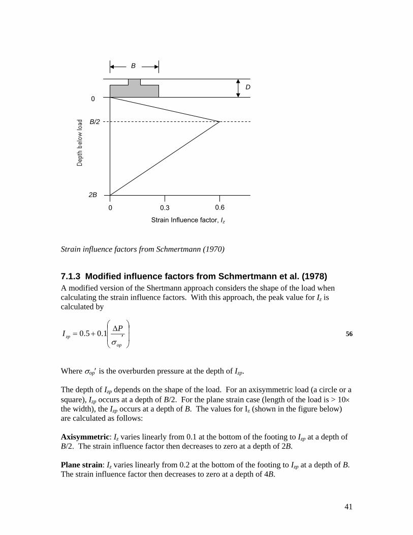
7.1.2 Influence factors from Schmertmann (1970) The simplest approach is to assume that the strain influence factor Iz increases linearly from zero at the bottom of the footing to a maximum of 0.6 at a depth of ½B below the footing where B is the footing width. The strain influence factor then decreases linearly to zero at a depth of 2B below the footing bottom. This distribution is shown below.

∑=

ΔΔ=

n

izi

si

it I

EzPCC

11δ

41

Strain influence factors from Schmertmann (1970)

7.1.3 Modified influence factors from Schmertmann et al. (1978) A modified version of the Shertmann approach considers the shape of the load when calculating the strain influence factors. With this approach, the peak value for Iz is calculated by

56

Where σop′ is the overburden pressure at the depth of Izp. The depth of Izp depends on the shape of the load. For an axisymmetric load (a circle or a square), Izp occurs at a depth of B/2. For the plane strain case (length of the load is > 10× the width), the Izp occurs at a depth of B. The values for Iz (shown in the figure below) are calculated as follows: Axisymmetric: Iz varies linearly from 0.1 at the bottom of the footing to Izp at a depth of B/2. The strain influence factor then decreases to zero at a depth of 2B. Plane strain: Iz varies linearly from 0.2 at the bottom of the footing to Izp at a depth of B. The strain influence factor then decreases to zero at a depth of 4B.

D

0.6

Strain Influence factor, Iz

B/2

2B

B

0

0 0.3

⎟⎟

⎠

⎞

⎜⎜

⎝

⎛

′Δ

+=op

zpPI

σ1.05.0

42

In Settle3D, Iz is calculated using the axisymmetric equations for circle and square loads. For rectangular loads in which the length is greater than ten times the width, the plane strain approach is used. For rectangular loads in which the length is less than ten times the width, a linear interpolation between the axisymmetric and plane strain case is performed, dependent on the length to width ratio.

Strain influence factors from Schmertmann et al. (1978).

7.1.4 Elastic modulus The elastic modulus Es can be estimated from the results of a Cone Penetration test: Es = 2.0qc Schmertmann (1970) Es = 2.5qc Modified Schmertmann (1978), Axisymmetric Footing Es = 3.5qc Modified Schmertmann (1978), Plane strain footing Where qc is the cone tip bearing resistance. As with the calculation of the strain influence factor, the value for Es is calculated to be between the axisymmetric case and plane strain

D

0.6

Strain Influence factor, Iz

B/2

2B

B

0

0 0.3

4B

B

0.1 0.2 0.5 0.4

Plane strain

Axisymmetric

43

case if the length of the load is less than ten times the width (for the modified Schmertmann calculations).

7.2 Peck, Hanson and Thornburn The method of Peck, Hanson and Thornburn (1974) uses the results of a Standard Penetration Test (SPT) to obtain settlement. The water table and overburden pressure at the location of the SPT are taken into account. Settlement results are obtained from matching the problem geometry and corrected SPT results to empirical curves.

7.2.1 SPT testing The Standard Penetration Test produces a value, N, equal to the number of hammer blows needed to drive an SPT sample 1 foot through the soil. Standards dictate the details of the procedure. To use the Peck, Hanson and Thornburn method, the N value should be corrected to account for the efficiency of your testing system. Peck et al., assume that a standard test is being performed in which 60% of the energy is transmitted to the soil. If your system is more or less efficient, a correction should be made:

57

Where,

N60 = the SPT N value corrected for field testing procedures N is the recorded number of blows per foot, Em is the hammer efficiency in percent (generally between 45-95)

Skempton (1986) proposes further corrections to account for the rod length and borehole diameter:

58

Where, Cb is the borehole diameter correction (Cb = 1.0 for borehole diameter less than 115 mm, 1.05 for borehole diameters between 115 and 150 mm and 1.15 if the diameter is > 150 mm) Cr is the rod length correction (Cr = 0.75 for less than 4 m of drill rods, 0.85 for 4-6 m of drill rods, 0.95 for 6-10 m, and 1.0 for drill rods more than 10 m) Other corrections are often performed to account for overburden pressure and the water table but these are generally method dependent and will be described separately for each method.

⎟⎠⎞

⎜⎝⎛=

6060mENN

⎟⎠⎞

⎜⎝⎛=

6060m

rbENCCN

44

7.2.2 Settlement calculation The settlement in inches is calculated by:

59

Where σL is the applied load, ΔP1 is the load required to produce a settlement of 1 inch and Cw is the correction factor for water table depth. The water table correction Cw is given by:

60

Where

zw is the depth to the water table D is the depth to the bottom of the load B is the load width.

The value for ΔP1 is obtained from the empirical charts shown below. To use the charts, a corrected blow count is required:

61

Where Cn is the correction for overburden pressure. The overburden correction is given by:

62

Where σod′ is the initial effective stress in tons/ft2 due to overburden soil. The value of (N60)′ represents the average value between the bottom of the footing and a depth of B below the bottom of the footing. So, if there are multiple layers, the overburden stress is calculated for the midpoint of each layer and the correction is calculated by equation 62. (N60)′ is then calculated for each layer. The average (N60)′ between depths of D and D+B is then calculated and used to get ΔP1 from the charts below. Once you have obtained (N60)′, use this value along with your footing width B and ratio of footing depth to width D/B to obtain ΔP1 from the charts below. This is then used in equation 59 to get the settlement. Settle3D automatically interpolates between the curves to obtain ΔP1.

wL CP1Δ

=σδ

1*5.05.0 ≤+

+= ww

w CBD

zC

( ) nCNN 6060 =′

220log77.0 ≤⎟⎟

⎠

⎞

⎜⎜

⎝

⎛′= n

od

n CCσ

45

Charts used for obtaining ΔP1, the load required to induce a settlement of 1 inch. The N value refers to the blow counts corrected for efficiency, overburden and water table. Reproduced from Peck, Hanson and Thornburn, 1974.

7.3 Schultze and Sherif This method, proposed by Schultze and Sherif (1973) is based on the equation for settlement in an elastic isotropic half-space:

63

Where σL is the loading stress,

B is the load width, Es is the one-dimensional modulus and fn is an influence factor that is a function of: ν – Poisson’s ratio L/B – load length divided by load width H/B – thickness of compressible layer divided by load width

The geometry of the problem is shown below. The contribution of Schultze and Sherif was to write this equation in terms of the blow counts, N60 instead of Es. Using empirical data, the following equation was derived:

64

The value for fn is taken from the charts shown below. This assumes that the Poisson’s ratio is 0. It is assumed that below a depth of 2B the influence of the load is minimal so for values of H/B > 2, the value of fn at H/B = 2 is used.

ns

L fE

Bσδ =

( ) ( )BDNBfnL

/4.0187.060 +

=σδ

46

The original equation in Schultze and Sherif (1973) is slightly different from that shown in equation 64. It was derived assuming 'stress' units of kg/cm2. However the associated fn curves are not given, therefore Settle3D uses a modified equation from U.S. Army Corps of Engineers (1990) which expects stress units of tons/ft2. The curves for fn from this reference are shown below.

Geometry of settlement problem for Schultze and Sherif solution

0

0.01

0.02

0.03

0.04

0.05

0.06

0.07

0.08

0.09

0.1

0.11

0 0.5 1 1.5 2

H/B

fn

5

L/B = 100

2

1

Charts used to calculate the settlement influence factor for the Schultze and Sherif method.

H

BD

σL

47

7.4 D'Appolonia Method This method was proposed by D'Appolonia et al (1968, 1970) based on elastic theory. Immediate settlement is calculated by:

65

where μ0 is the embedment influence factor μ1 is the compressible strata influence factor σL is the loading stress B is the load width Es is the one-dimensional modulus The embedment influence factor, μ0, is a function of the ratio of footing depth to load width (D/B). A relationship was proposed by D'Appolonia et al however a more accurate version was derived by Christian and Carrier (1978) as shown in the figure below. This is the version used by Settle3D. The compressible strata influence factor, μ1, is a function of the ratio of compressible layer thickness to load width (H/B) and load length to load width (L/B). As with μ0, the more accurate version of Christian and Carrier (1978) is used by Settle3D. This relationship is shown below.

Charts used to calculate μ0 and μ1 for the D'Appolonia method. From Christian and Carrier (1978).

s

L

EBσμμδ 10=

48

The one-dimensional modulus is obtained from SPT blow count values using the empirical relationship shown below.

Relationship between 1D modulus of compressibility and SPT blow counts. From D'Appolonia et al (1970).

8 References Abid, M.M. and Pyrah, I.C., 1988. Guidelines for using the finite element method to predict one-dimensional consolidation behaviour, Computers and Geotechnics, 5, 213-226. Barron, R.A., 1948. Consolidation of fine-grained soils by drain wells, Trans. Am. Soc. Civ. Eng., 113, 718-742. Christian, J.T. and Carrier, W.D., 1978. Janbu, Bjerrum and Kjaernsli's chart reinterpreted, Canadian Geotechnical Journal, 15, 123-128. Coduto, D.P., 1999. Geotechnical Engineering, Principles and Practices, Prentice-Hall Inc., Upper Saddle River, New Jersey. D'Appolonia, D.J., D'Appolonia, E., Brissette, R.F., 1968. Settlement of spread footings on sand. ASCE Journal of Soil Mechanics & Foundations Division, 94 (SM3), 735-760. D'Appolonia, D.J., D'Appolonia, E., Brissette, R.F., 1970. Closure to "Settlement of spread footings on sand", ASCE Journal of Soil Mechanics & Foundations Division, 96 (SM2), 735-760.

49

Hansbo, 1979. Consolidation of clay by band-shaped prefabricated drains. Ground Engng., 12 (5). Hansbo, S., 1981. Consolidation of fine-grained soils by prefabricated drains, Proc. 10th Int. Conf. on Soil Mechanics and Foundation Engineering, Balkema, Rotterdam, 3, 677-682. Janbu, N., 1963. Soil compressibility as determined by oedometer and triaxial tests. European Conference on Soil Mechanics and Foundation Engineering, Wiesbaden, Vol. 1, pp. 19-25, andVol. 2, pp. 17-21. Janbu, N., 1965. Consolidation of clay layers based on non-linear stress-strain. Proceedings 6th International Conference on Soil Mechanics and Foundation Engineering, Montreal, Vol. 2, pp. 83-87. Kjellman, W. 1948. Consolidation of fine-grained soils by drain wells. Trans. ASCE, Vol. 113, Contribution to the discussion. Koppejan, A.W., 1948. A formula combining the Terzaghi load compression relationship and the Buisman secular time effect, Proc. 2nd Int. Conf. Soil Mech. And Found. Eng., Rotterdam, 3, 32-38. Lambe, T.W. and Whitman, R.V., 1969. Soil Mechanics, John Wiley and Sons. Mesri, G., Ajlouni, M.A., Feng, T.W. and Lo, D.O.K., 2001. Surcharging of soft ground to reduce secondary settlement, Proceedings of the 3rd International Conference on Soft Soil Engineering, 55-65. Mesri, G., Stark, T.D., Ajlouni, M.A. and Chen, C.S., 1997. Secondary compression of peat with or without surcharging, Journal of Geotechnical and Geoenvironmental Engineering, 123, 411-421. Peck, R.B., Hanson, W.E. and Thornburn, T.H., 1974. Foundation Engineering, 2nd edition, John Wiley and Sons, Inc. Schmertmann, J. H. 1970. Static Cone to Compute Static Settlement Over Sand, Journal of the Soil Mechanics and Foundations Division, ASCE, 96, 1011-1043. Schmertmann, J. H., Hartmann, J.P., and Brown, P.R. 1978. Improved strain influence factor diagrams, Journal of the Geotechnical Engineering Division, ASCE, 104, 1131-1135. Schultze, E. and Sherif, G. 1973. Prediction of settlements from evaluated settlement observations for sand. Proceedings of the 8th Int. Conf. Soil Mech. Foundation Eng., Moscow, v1.3, 225-230.

50

Skempton, A.W., 1954. The pore-pressure coefficients A and B, Geotechnique, 4, 143-147. Skempton, A.W., 1986. Standard penetration test procedures and the effects in sands of overburden pressure, relative density, particle size, aging and overconsolidation. Geotechnique, 36, 425-447. Tavenas, F., Jean, P., Leblond, P. and Leroueil, S., 1983. The permeability of natural soft clays. II Permeability characteristics, Canadian Geotechnical Journal, 20, 645-550. Terzaghi, K., Peck, R.B. and Mesri, G., 1996. Soil mechanics in engineering practice, 3rd ed., Wiley, New York. U.S. Army Corps of Engineers (1990). Settlement Analysis: Engineer Manual 1110-1-1904. Washington DC. van Baars, S., 2003. Soft soil creep modelling of large settlements, 2nd International Conference on Advances in Soft Soil Engineering and Technology, Kuala Lumpur, Malaysia. Vaughan, P.R., 1989. Non-linearity in seepage problems – theory and field observation. Del Mello Volume, Edgard Blucher Ltda., Sau Paulo, Brasil, 501-516. Venkatramaiah, C. (2006). Geotechnical Engineering, Revised Third Edition, New Age International, New Delhi, pp. 419 – 435. Vijaykumar, S., Yacoub, T.E. and Curran, J.H., 2000. A node-centric indirect boundary element method: three-dimensional displacement discontinuity, Comput. Struct, 74, 687-703. Vijaykumar, S., Yacoub, T.E. and Curran, J.H., 2009. Solution of Rigid Foundation Problems Using an Error Minimization, to be submitted for publication. Yue, Z. Q., 1995. On generalized Kelvin solution in multilayered elastic medium, J. Elasticity, 40 (1), 143. Yue, Z. Q., 1996. On elastostatics of multilayered solids subjected to general surface traction, Quart. J. Mech. Appl. Math. 49 (Part 3), 471-499.

51

9 Table of symbols σ Total stress (vertical) σ′ Effective stress (vertical) σi′ Initial or in-situ effective stress (vertical) σL Loading stress σM Mean stress γ Soil unit weight γwater Unit weight of water ν Poisson’s ratio ε Strain (vertical) δ Settlement (vertical displacement) μ0 Embedment influence factor (D'Appolonia method) μ1 Compressible strata influence factor (D'Appolonia method) a Janbu stress exponent B or B Skempton pore pressure coefficient or load width Cα Secondary compression index Cαγ Strain based secondary compression index Cαγr Strain based secondary recompression index Cαr Secondary recompression index Cc Compression index Ccγ Strain based compression index Cp Koppejan compression index C′p Koppejan recompression index Cr Recompression index Crγ Strain based recompression index Cs Koppejan compression index for secondary consolidation C′s Koppejan recompression index for secondary consolidation ch Horizontal coefficient of consolidation cv Coefficient of consolidation (vertical) cvr Recompression coefficient of consolidation (vertical) d Equivalent drain diameter D Drain spacing or load depth De Equivalent drain spacing ds Diameter of smear zone E Young’s modulus Es One-dimensional Young’s modulus Esur Unload-reload 1D Young’s modulus e Void ratio e0 Initial void ratio ep Void ratio at the end of primary consolidation H Layer thickness h Sublayer thickness k Permeability (vertical)

52

kh Horizontal permeability kr Recompression permeability (vertical) L Load length l Drain length Moc Janbu overconsolidated modulus m Janbu modulus number mr Janbu recompression modulus number mv One-dimensional compressibility mvur Unload-reload 1D compressibility N Blow counts from SPT test N60 Blow counts corrected to 60% efficiency (N60)′ N60 corrected for overburden stress and water table OCR Overconsolidation ratio Pc Preconsolidation stress qw Drain discharge capacity S Ratio of smear zone diameter to drain diameter t Time u Pore water pressure ue Excess pore water pressure z Depth