Setting-less Protection: Laboratory Testing · Setting-less Protection: ... Application to Three...

Setting-less Protection:Laboratory Testing

Final Project Report

Power Systems Engineering Research Center

Empowering Minds to Engineerthe Future Electric Energy System

Setting-less Protection: Laboratory Testing

Final Project Report

Project Team

Sakis A. P. Meliopoulos, Project Leader George J. Cokkinides

Georgia Institute of Technology

Graduate Research Assistants

Rui Fan, Renke Huang, Yonghee Lee Liangyi Sun, and Zhenyu Tan

Georgia Institute of Technology

PSERC Publication 14-03

June 2014

For information about this project, contact: Sakis A.P. Meliopoulos Georgia Institute of Technology School of Electrical and Computer Engineering Atlanta, Georgia 30332-0250 Phone: 404-894-2926 E-mail: [email protected] Power Systems Engineering Research Center The Power Systems Engineering Research Center (PSERC) is a multi-university Center conducting research on challenges facing the electric power industry and educating the next generation of power engineers. More information about PSERC can be found at the Center’s website: http://www.pserc.org. For additional information, contact: Power Systems Engineering Research Center Arizona State University 527 Engineering Research Center Tempe, Arizona 85287-5706 Phone: 480-965-1643 Fax: 480-965-0745 Notice Concerning Copyright Material PSERC members are given permission to copy without fee all or part of this publication for internal use if appropriate attribution is given to this document as the source material. This report is available for downloading from the PSERC website.

2014 Georgia Institute of Technology. All rights reserved.

1

Acknowledgements

This is the final report for the Power Systems Engineering Research Center (PSERC) research project T-52G titled “Setting-less Protection”. This targeted PSERC research project was funded by EPRI. We express our appreciation to EPRI, and especially to Paul Myrda, Technical Executive, EPRI, for his support and guidance. We also express our appreciation for the support provided by PSERC’s industrial members, EPRI members, and the National Science Foundation’s Industry / University Cooperative Research Center program. The authors wish to recognize the postdoctoral researchers and graduate students at the Georgia Institute of Technology who contributed to the research and creation of project reports:

• Rui Fan • Renke Huang • Yonghee Lee • Liangyi Sun • Zhenyu Tan.

i

Executive Summary

Present day numerical relays use high end microprocessors for implementing multiple functions of protection, thereby providing many more options for improved protection. At the same time, the additional options have created increased complexity and increased possibilities of human errors, while the basic nature of the problem of selecting settings has remained the same. For example, a transformer protection relay may include all the typical protection functions that traditionally used with electromechanical relays, such as differential, over-current, and voltage over frequency. Since these functions work independently, even if they are implemented on the same relay, they suffer from the same limitations as the common, single relay/single function approach. Each function must be set separately to meet a specified criteria, but the settings must be coordinated with other protective devices. The coordinated settings are typically selected to satisfy requirements that are often conflicting, meaning that compromise settings must be chosen. Because of these compromise settings, occasionally fault conditions can lead to an undesirable relay response. In addition, despite the progress of the last few decades, some protection gaps persist. For instance, we still do not have 100% reliable approaches for certain fault types, such as high impedance faults and faults near neutrals. Setting-less protection based on dynamic state estimation is an emerging technology that effectively uses advances in numerical relays to improve protection. This protection approach uses simplified settings, just the operating limits of devices. For this reason it was named “setting-less.” A more descriptive name is coordination-less protection. The dynamic state estimation approach requires that complex analytics be performed on data acquired by the data acquisition system of a relay. The setting-less protection method was inspired from the fact that differential protection is one of the most secure protection schemes that we have and does not require coordination with other protection function. Differential protection simply monitors the validity of Kirchoff's current law in a device, i.e., the weighted sum of the currents going into a device must be equal to zero. This concept can be generalized into monitoring the validity of all other physical laws that the device must satisfy, such as Kirchoff's voltage law and Faraday's law. This monitoring can be done in a systematic way by use of dynamic state estimation. Dynamic state estimation is used to continuously monitor the dynamic model of the component under protection. Specifically, all the physical laws that a component must obey are expressed in the dynamic model of the component. The monitoring system of the component under protection that continuously measures terminal data (such as the terminal voltage magnitude and angle, the frequency, the rate of frequency change), and other variables (such as temperature and speed), and component status data (such as tap setting and breaker status). The dynamic state estimation processes these measurements and extracts the real time dynamic model of the component and its operating conditions. If any one of the physical laws for the component under protection is violated, dynamic state estimation will identify this condition. Thus, the dynamic state estimator extracts the real-time dynamic model of the component under protection to determine whether the physical laws for the component are being satisfied. The dynamic model of the component accurately reflects the current operating condition of the

ii

component. The decision to trip or not to trip the component is based only on the condition of that component irrespective of the condition (such as faults) of other system components. In prior research, numerical experiments based on the setting-less protection approach were performed on a number of protection problems, specifically, transmission line protection, capacitor bank protection, transformer protection, reactor protection, induction motor protection and distribution line protection. The research demonstrated that the dynamic state estimation approach provides a secure and dependable protection scheme, and does not require coordination with other devices or protection schemes while, at the same time, addresses many protection gaps. Following the above positive results from numerical experiments, the method has been refined further and tested in the laboratory. This report summarizes the methodological refinements and the results of further laboratory testing of their application. The analytics of the setting-less protection are complex. To provide a practical approach to setting-less protection, the analytics have been “objectified”. Specifically, the basic building blocks of the setting-less protection algorithm have been mathematically abstracted to form objects that are recognizable by a single computational algorithm. The implementation is based on merging unit technology. This report describes:

• Methodology refinements • Laboratory setup and experiments to test the refinements • Test results.

The results continue to show that setting-less protection is a viable approach to system protection.

iii

Table of Contents

1. Introduction ........................................................................................................................... 1 2. Brief Review of the DSE Based Protection........................................................................... 3 3. Implementation of Setting-less Protection ............................................................................ 7

3.1. Protection Zone Mathematical Model .............................................................................. 8 3.2. Object-Oriented Measurements ........................................................................................ 9 3.3. Object-Oriented Dynamic State Estimation ................................................................... 11 3.4. Bad Data Detection and Identification ........................................................................... 12 3.5. Protection Logic / Component Health Index .................................................................. 12 3.6. Online Parameter Identification ..................................................................................... 13 3.7. Summary and Comments ............................................................................................... 13

4. Laboratory Implementation and Testing ............................................................................. 15 4.1. Laboratory Implementation ............................................................................................ 15 4.2. Testing Procedure – User Interface ................................................................................ 16 4.3. Application to Capacitor Bank Protection ...................................................................... 19

4.3.1. Capacitor Bank: Test case 1 – Internal fault 1 ......................................................... 24 4.3.2 Capacitor Bank: Test case 2 – Internal fault 2 ......................................................... 26

4.4. Application to Single Section Transmission Line Protection ......................................... 28 4.4.1. Single Section Transmission Line: Test case - High Impedance Fault, Low Impedance Fault, External Fault, External Breaker Operation ........................................... 31

4.5. Application to Multi-section Transmission Line Protection .......................................... 33 4.5.1 Multi-section Transmission Line: Test case – Internal fault ................................... 38

4.6. Application to Single Phase Saturable Core Variable Tap Transformer Protection ...... 41 4.6.1. Transformer: Test case 1- Energization ................................................................... 49 4.6.2. Transformer: Test case 2- Source Switching ........................................................... 50 4.6.3. Transformer: Test case 3- Internal Fault .................................................................. 52

4.7. Application to Three Phase Saturable Core Reactor Protection ..................................... 54 4.7.1 Reactor: Test case .................................................................................................... 59

5. References ........................................................................................................................... 61 Appendix A: Overall Design of the Setting-less Relay ................................................................ 62 Appendix B: Object-Oriented Implementation ............................................................................. 64

B1. Time Domain SCAQCF Device Model Description ...................................................... 64 B2. Time Domain SCAQCF Measurement Model Description ........................................... 65 B3. Measurement Definition ................................................................................................. 67

B3.1. Actual Measurement ................................................................................................ 67 B3.2. Virtual Measurement ............................................................................................... 67 B3.3. Pseudo Measurement ............................................................................................... 68 B3.4. Derived Measurement .............................................................................................. 68

B4. Sparsity Based State Estimation Algorithm ................................................................... 69 B5. Frequency Domain SCAQCF Device Model Description ............................................. 74 B6. Frequency Domain SCAQCF Measurement Model Description ................................... 75

iv

Table of Contents (continued) Appendix C: Time Domain SCAQCF Model – Capacitor Bank .................................................. 77

C1. Three Phase Capacitor Bank Compact Model ................................................................ 77 C2. Three Phase Capacitor Bank Quadratized Model .......................................................... 78 C3. Three Phase Capacitor Bank SCAQCF Device Model .................................................. 79 C4. Three Phase Capacitor Bank SCAQCF Measurement Model ........................................ 86

Appendix D: Time Domain SCAQCF Model – Single Section Transmission Line Protection ... 93

D1. Three Phase Transmission Line Compact Model ........................................................... 93 D2. Three Phase Transmission Line Quadratized Model ...................................................... 94 D3. Three Phase Transmission Line SCAQCF Device Model ............................................. 95 D4. Three Phase Transmission Line SCAQCF Measurement Model ................................... 99

Appendix E: Time Domain SCAQCF Model – Multi-section Transmission Line Protection ... 103

E1. Construction of Multi-section Transmission Line SCAQCF Model ............................ 103 E2. Three Phase Multi-section Transmission Line SCAQCF Model ................................. 104 E3. Three Phase Multi-section Transmission Line SCAQCF Measurement Model .......... 114

Appendix F: Time Domain SCAQCF Model – Single Phase Saturable Core Variable Tap Transformer Protection ............................................................................................................... 118

F1. Single Phase Saturable Core Transformer Compact Model ......................................... 118 F2. Single Phase Saturable Core Transformer Quadratic Model ....................................... 120 F3. Single Phase Saturable Core Transformer SCAQCF Device Model ........................... 122 F4. Single Phase Saturable Core Transformer SCAQCF Measurement Model ................. 140

Appendix G: Time Domain SCAQCF Model – Three Phase Saturable Core Reactor Protection .................................................................................................................................... 155

G1. Three Phase Saturable Core Three Phase Reactor Compact Model Description ......... 155 G2. Three Phase Saturable Core Three Phase Reactor Quadratized Model Description .... 156 G3. Three Phase Saturable Core Three Phase Reactor SCAQCF Device Model Description 160 G4. Three Phase Saturable Core Three Phase Reactor SCAQCF Measurement Model ..... 172

v

List of Figures

Figure 2.1: Illustration of Setting-less Component Protection Scheme .......................................... 4 Figure 2.2: Illustration of Setting-less Protection Logic ................................................................. 5 Figure 2.3:Overall Approach for Component Protection ............................................................... 6 Figure 3.1: Setting-Less Protection Relay Organization ................................................................ 7 Figure 3.2: Example Derived Measurements................................................................................ 11 Figure 3.3: Confidence Level (%) vs Parameter k ........................................................................ 13 Figure 4.1: Lab Implementation Illustration ................................................................................. 15 Figure 4.2: Setting-less Protection Relay User Interface .............................................................. 16 Figure 4.3: MU Data Concentrator User Interface ....................................................................... 18 Figure 4.4: User Interface for the Measurement Channel of the Merging Unit ........................... 19 Figure 4.5: Three Phase Capacitor Bank Example ....................................................................... 19 Figure 4.6: Three Phase Capacitor Bank Simplified Model (C is the net capacitance of a phase) ............................................................................................................................................ 20 Figure 4.7: Test System for Capacitor Bank Simulations............................................................. 24 Figure 4.8: Topology of the Capacitor Bank and Location of Measurements.............................. 25 Figure 4.9: Results of the Capacitor Bank Setting-less Protection ............................................... 26 Figure 4.10: Topology of the Capacitor Bank and Location of Measurements ............................ 27 Figure 4.11: Results of the Capacitor Bank Setting-less Protection ............................................. 28 Figure 4.12: Three Phase Short Transmission Line Compact Model ........................................... 29 Figure 4.13:Test System for Transmission Line Simulations ....................................................... 31 Figure 4.14: Configuration of the Transmission Line .................................................................. 32 Figure 4.15: Results of the Singe Section Transmission Line Setting-less Protection ................. 33 Figure 4.16: Three Phase Short Transmission Line Compact Model ........................................... 34 Figure 4.17: Three Phase Multi-section Transmission Line Compact Model .............................. 34 Figure 4.18: Test System for Multi-section Transmission Line ................................................... 39 Figure 4.19: Location of Measurements at TABL side ................................................................ 40 Figure 4.20: Location of Measurements at VACA side ............................................................... 40 Figure 4.21: Results of the Three Phase Multi-section Transmission Line Setting-less Protection ...................................................................................................................................... 41 Figure 4.22: Single-Phase Transformer Compact Model ............................................................. 42 Figure 4.23: Energization Situation for Single Phase Transformer .............................................. 49 Figure 4.24: Results of Setting-less Protection for Transformer Energization Situation ............. 50 Figure 4.25: Source Switching Situation for Single Phase Transformer ...................................... 51 Figure 4.26: Results of Setting-less Protection for Transformer Source Switching Situation ..... 52 Figure 4.27: Internal Fault Situation for Single Phase Transformer ............................................. 53 Figure 4.28: Results of Setting-less Protection for Single Phase Transformer ............................. 53 Figure 4.29: Three Phase Saturable Core Reactor Model ............................................................. 54 Figure 4.30: Test System for Three Phase Saturable Core Reactor .............................................. 60

vi

List of Figures (continued) Figure 4.31: Results of Setting-less Protection for Three Phase Saturable Core Reactor ............ 60 Figure A.1: Overall Design of Setting-less Protection Relay ....................................................... 62 Figure B.1: Flow Chart of Object-Oriented Setting-less Protection for Linear Case ................... 72 Figure B.2: Flow Chart of Object-Oriented Setting-less Protection for Nonlinear Case ............. 73 Figure C.1: The Three Phase Capacitor Bank Circuit Model ....................................................... 77 Figure D.1: The Three Phase Transmission Line Circuit Model .................................................. 93 Figure E.1: Three Phase Multi-section Transmission Line Compact Model .............................. 103 Figure F.1: Single Phase Transformer Equivalent Circuit .......................................................... 118 Figure G.1: Three Phase Reactor Model..................................................................................... 155

vii

1. Introduction

Present day numerical relays use high end microprocessors for implementing multiple functions of protection. For example a transformer protection relay may include all the typical protection functions that traditionally used with electromechanical relays, i.e., differential, over-current, V/Hz function, etc. Since these functions work independently, even if they are implemented on the same relay, they suffer from the same limitations as the usual single relay/single function approach. Each function must be set separately but the settings must be coordinated with other protective devices. The coordinated settings are typically selected so that can satisfy requirements that many times are conflicting and therefore a compromise must be selected. For this reason, most of the time the settings represent a compromise and occasionally may exist possible fault conditions that may lead to an undesirable relay response. It should be understood that numerical relays have provided many more options that have improved the above procedure. At the same time the additional options have created increased complexity and increased possibilities of human errors, while the basic nature of the problem of selecting settings has remained the same: the settings must be selected to satisfy criteria that many times are conflicting. The natural question is whether any new technologies and trends can favorably affect the protection process. There are technologies that can enable better, integrated approach to the overall protection. Some of these technologies are (technology is in flux with many developments still to occur):

1. Merging units/separation of data acquisition and data processing/protection 2. GPS synchronized measurements (PMUs) 3. Data Concentrator (PDCs, switches, etc.) 4. Smarter sensors 5. Integrated (power system/relay) analysis programs that enable faster and more reliable

assessment of settings 6. Data validation/state extraction 7. Other

It is difficult to assess the full impact of these technologies on the future of protection. One thing is clear though: while there is much technology development in hardware and the capabilities of hardware, the development of new approaches to fully utilize the new capabilities is lagging. This is the classical problem of "hardware being ahead of software". This will come with realistic assessment of the new technologies and bold experimentation of new approaches and the eventual emergence of successful approaches. The existence of the above technologies and the quest for better more reliable (secure and dependable) protection has led to the investigation of dynamic state estimation protection approaches. This investigation has shown that it is possible to develop a protection approach that does not require coordination with other protection functions and at the same time address many protection gaps. The investigation has been carried out with many numerical experiments and has been reported in the previous year report.

1

Following the above investigation and the positive results, the method has been further refined and also tested in the laboratory. This report summarizes the method refinements and its application in the laboratory.

2

2. Brief Review of the DSE Based Protection

For secure and reliable protection of power components such as a generator, line, transformer, etc. a new approach has emerged based on component health dynamic monitoring. The proposed method uses dynamic state estimation [4-7], based on the dynamic model of the component, which accurately reflects the nonlinear characteristics of the component as well as the loading and thermal state of the component. For more secure protection of protection zones such as transmission lines, transformers, capacitor banks, motors, generators, generator/transformer unit, etc., this report proposes a new method. The method has been inspired from the fact that differential protection is one of the most secure protection schemes that we have and it does not require coordination with other protection function. Differential protection simply monitors the validity of Kirchoff's current law in a device, i.e., the weighted sum of the currents going into a device must be equal to zero. This concept can be generalized into monitoring the validity of all other physical laws that the device must satisfy, such as Kirchoff's voltage law, Faraday's law, etc. This monitoring can be done in a systematic way by the use of dynamic state estimation. Specifically, all the physical laws that a component must obey are expressed in the dynamic model of the component. Dynamic state estimation is used to continuously monitor the dynamic model of the component (zone) under protection. If any of the physical laws for the component under protection is violated, the dynamic state estimation will capture this condition. Thus, it is proposed to use dynamic state estimator to extract the dynamic model of the component under protection [2-5] and to determine whether the physical laws for the component are satisfied. The dynamic model of the component accurately reflects the condition of the component and the decision to trip or not to trip the component is based on the condition of the component only irrespectively of the condition (faults, etc.) of other system components. The proposed method requires a monitoring system of the component under protection that continuously measures terminal data (such as the terminal voltage magnitude and angle, the frequency, and the rate of frequency change - this task is identical to present day numerical relays), other variables such as temperature, speed, etc., as appropriate, and component status data (such as the tap setting, breaker status, etc.). The dynamic state estimation processes these measurements and extracts the real time dynamic model of the component and its operating conditions.

3

Figure 2.1: Illustration of Setting-less Component Protection Scheme

After estimating the operating conditions, the well-known chi-square test [6] calculates the probability that the measurement data are consistent with the component model, i.e., the physical laws that govern the operation of the component. In other words, this probability, which indicates the confidence level of the goodness of fit of the component model to the measurements, can be used to assess the health of the component. The high confidence level indicates a good fit between the measurements and the model, which indicates that the operating condition of the component is normal. However, if the component has internal faults, the confidence level would be almost zero (i.e., the very poor fit between the measurement and the component model). Figure 2.1 shows the concept of entire proposed protection scheme. In general, the proposed method can identify any internal abnormality of the component within a cycle and trip the component immediately. Furthermore, it does not degrade the security because a relay does not trip in the event of normal behavior of the component, for example, in case of transformer protection, inrush currents or over excitation currents, since in these cases, as long as the inrush currents are consistent with the transient behavior of the transformer as dictated by the dynamic model, the method will produce a high confidence level that the transients are consistent with the model of the component. Note also that the method does not require any settings or any coordination with other relays. It is important to note that the proposed scheme will perform best when: (a) the measurements are as accurate as possible - dependent on the type of instrument transformer used, i.e., VT, CT, etc. and the instrumentation channel, i.e., control cable, etc. and (b) the accuracy of the dynamic model of the component under protection. These issues, while important, are beyond the scope of this report. These issues will be addressed in a subsequent report.

4

Figure 2.2: Illustration of Setting-less Protection Logic

The proposed protection logic is briefly illustrated in Figure 2.2. The method requires a monitoring system of the component under protection that continuously measures terminal data (such as the terminal voltage magnitude and angle, the frequency, and the rate of frequency change) and component status data (such as tap setting (if transformer) and temperature). The dynamic state estimation processes these measurement data with the dynamic model of the component yielding the operating conditions of the component. This approach faces some challenges which can be overcome with present technology. A partial list of the challenges is given below:

1. Ability to perform the dynamic state estimation in real time 2. Initialization issues 3. Communications in case of a geographically extended component (i.e., lines) 4. New modeling approaches for components - connects well with the topic of modeling 5. Requirement for GPS synchronized measurements in case of multiple independent data

acquisition systems. 6. Other

The modeling issue is fundamental in this approach. For success the model must be high fidelity so that the component state estimator will reliably determine the operating status (health) of the component. For example consider a transformer during energization. The transformer will experience high in-rush current that represent a tolerable operating condition and therefore no relay action should occur. The component state estimator should be able to "track" the in-rush current and determine that they represent a tolerable operating condition. This requires a transformer

5

model that accurately models saturation and in-rush current in the transformer. We can foresee the possibility that a high fidelity model used for protective relaying can be used as the main depository of the model which can provide the appropriate model for other applications. For example for EMS applications, a positive sequence model can be computed from the high fidelity model and send to the EMS data base. The advantage of this approach will be that the EMS model will come from a field validated model (the utilization of the model by the relay in real time provide the validation of the model). This overall approach is shown in Figure 2.3. Since protection is ubiquitous, it makes economic sense to use relays for distributed model data base that provides the capability of perpetual model validation.

Figure 2.3:Overall Approach for Component Protection

6

3. Implementation of Setting-less Protection

The implementation of the setting-less protection has been approached from an object orientation point of view. For this purpose the constituent parts of the approach have been evaluated and have been abstracted into a number of objects. Specifically, the setting-less approach requires the following objects:

1. the mathematical model of the protection zone 2. the physical measurements that may consist of analog and digital data 3. the mathematical model of the physical measurements 4. the mathematical model of the virtual measurements 5. the mathematical model of the derived measurements 6. the mathematical model of the pseudo measurements 7. the dynamic state estimation algorithms 8. the bad data detection and identification algorithm 9. the protection logic and trip signals 10. online parameter identification method

The last task has not been addressed in the report but it is an integral part of the overall approach as in many cases it will be necessary to fine tune the model of the protection zone via online parameter identification methods. An overview of the design of the setting-less protection relay is shown in Figure 3.1.

Protection Zone SACQCF model

MeasurementDefinition

• Create Actual Measurement Model

• Create Virtual Measurement Model

• Create Pseudo Measurement Model

• Create Derived Measurement Model

SCAQCF Measurement Model

Setting-less Protection

Dynamic State Estimation

Error Analysis Bad Data

Detection & Identification

Model Parameter

Identification

Future

ProtectionLogic

Merging Unit

Merging Unit

Merging Unit

DataConcentrator

Figure 3.1: Setting-Less Protection Relay Organization

The setting-less protection algorithms have been streamlined for the purpose of increasing efficiency. An object-oriented approach for the DSE based protection algorithm is developed by utilizing the State and Control Algebraic Quadratic Companion Form (SCAQCF). All the

7

mathematical models of the apparatus in the power system are written in SCAQCF format so that the DSE based protection algorithm could be applied to any device. The algorithm automatically formulates the measurement model in the SCAQCF syntax from the SCAQCF device model and the measurement definition file, as illustrated by Figure 3.1. A data concentrator is utilized to align data from multiple merging units with the same time stamp and feed the streaming data into the DSE based protection module. The DSE based protection scheme continuously monitors the SCAQCF model of the component (zone) under protection by fitting the real-time measurement data to the measurement model in the SCAQCF syntax. If any of the physical laws for the component under protection is violated, the dynamic state estimation will capture this condition. Under normal operation, the device estimated measurement data from DSE should be exactly the same as the real measurement data. The mismatch between real measurements and estimated measurements indicates abnormalities in the device, then diagnose or trip decision should be made. Detailed implementation of setting-less protection in an object-oriented way is shown in Appendix A and Appendix B. This section gives a brief introduction of how setting-less protection is implemented.

3.1. Protection Zone Mathematical Model The mathematical model of the protection zone is required in a standard form. A standard has been defined in the form of the State and Control Algebraic Quadratic Companion Form (SCAQCF) and in a specified syntax to be defined later. The SCAQCF for a specific protection zone is derived with three computational procedures. Specifically, the dynamic model of a protection zone consists of a set of algebraic and differential equations. We refer to this model as the compact model of the protection zone. Subsequently this model is quadratized, i.e., in case there are nonlinearities of order greater than 2, additional state variables are introduced so that at the end the mathematical model consists of a set of linear and quadratic equations. We refer to this model as the quadratized model. Finally, the quadratized model is integrated using the quadratic integration method which converts the quadratized model of the protection zone into a set of algebraic (quadratic) function. This model is cast into a generalized Norton form. We refer to this model as the Algebraic Quadratic Companion Form. Since the variables in this AQCF contain all states and controls, thus it is named State and Control Algebraic Quadratic Companion Form. The standard State and Control Algebraic Quadratic Companion Form is obtained with two procedures: (a) model quadratization, and (b) quadratic integration. The model quadratization reduces the model nonlinearities so that the dynamic model will consist of a set of linear and quadratic equations. The quadratic integration is a numerical integration method that is applied to the quadratic model assuming that the functions vary quadratically over the integration time step. The end result is an algebraic companion form that is a set of linear and quadratic algebraic equations that are cast in the following standards form:

( , )

0T i T i T i

eqx eqx equ equ eqxu eq

I

Y F Y F F B

= + + + + −

x u

x x x u u u x u

(1)

8

where ( , )I x u is the through variable (current) vector, [ ( ), ( )]mt t=x x x is the external and internal

state variables, [ ( ), ( )]mt t=u u u is the control variables, t is present time, tm is the midpoint between the present and previous time, Yeq admittance matrix, Feq nonlinear matrices, and

( ) ( ) ( )eq eqx equ eq eqB N t h N t h M I t h K= − − − − − − −x u (2) The derivation of the standard State and Control Algebraic Quadratic Companion Form for specific protection zones is provided in the appropriate reports that describe the application of the setting-less protection schemes for specific protection zones. This standardization allows the object oriented handling of measurements in state estimation; in addition it converts the dynamic state estimation into a state estimation that has the form of a static state estimation.

3.2. Object-Oriented Measurements Any measurement, i.e., current, voltage, temperature, etc. can be viewed as an object that consists of the measured value and a corresponding function that expresses the measurement as a function of the state of the component. This function can be directly obtained (autonomously) from the State and Control Algebraic Quadratic Companion Form of the component. Because the algebraic companion form is quadratic at most, the measurement model will be also quadratic at most. Thus, the object-oriented measurement model can be expressed as the following standard equation:

,)(

)()(

)()(

)()()(

,,,

,,,

,,

kk

jimjmi

ktmji

jiji

ktji

imi

ktmi

ii

ktik

tc

txtxb

txtxb

txatxatz

η++

⋅⋅+

⋅⋅+

⋅+⋅=

∑

∑

∑∑

, (3)

where z is the measured value, t the present time, tm the midpoint between the present and previous time, x the state variables, a the coefficients of linear terms, b the coefficients of nonlinear terms, c the constant term, and η the measurement error. The measurements can be identified as: (a) actual measurements, (b) virtual measurements, (c) derived measurements and (d) pseudo measurements. The types of measurements will be discussed next. Actual Measurements: In general the actual measurements can be classified as across and through measurements. Across measurements are measurements of voltages or other physical quantities at the terminals of a protection zone such as speed on the shaft of a generator/model. These quantities are typically states in the model of the component. For this reason, the across measurements has a simple model as follows:

j i j jz x x η= ± + . (4)

9

Through measurements are typically currents at the terminals of a device or other quantities at the terminals of a device such as torque on the shaft of a generator/motor. The quantity of a through measurement is typically a function of the state of the device. For this reason, the through measurement model is extracted from the algebraic companion form, i.e., the measurement model is simply one equation of the SCACQF model, as follows:

, , , , , ,, , ,

k k k k k kj eqx i i eqx ij i j equ i i equ ij i j eqxu ij i j eq i

i i j i i j i j iz Y x F x x Y u F u u F x u b= ⋅ + ⋅ ⋅ + ⋅ + ⋅ ⋅ + ⋅ ⋅ −∑ ∑ ∑ ∑ ∑ ∑ , (5)

where the superscript k means the kth row of the matrix or the vector. Virtual Measurements: The virtual measurements represent a physical law that must be satisfied. For example we know that at a node the sum of the currents must be zero by Kirchoff’s current law. In this case we can define a measurement (sum of the currents); note that the value of the measurement (zero) is known with certainty. This is a virtual measurement. The model can provide virtual measurements in the form of equations that must be satisfied. Consider for example the mth SCAQCF model equation below:

, , , , , ,, , ,

0 k k k k k keqx i i eqx ij i j equ i i equ ij i j eqxu ij i j eq i

i i j i i j i j iY x F x x Y u F u u F x u b= ⋅ + ⋅ ⋅ + ⋅ + ⋅ ⋅ + ⋅ ⋅ −∑ ∑ ∑ ∑ ∑ ∑ (6)

This equation is simply a relationship among the states the component that must be satisfied. Therefore we can state that the zero value is a measurement that we know with certainty. We refer to this as a virtual measurement. Derived Measurements: A derived measurement is a measurement that can be defined for a physical quantity by utilizing physical laws. An example derived measurement is shown in Figure 3.2. The figure illustrates a series compensated power line with actual measurements on the line side only. Then derived measurements are defined for each capacitor section. Note that the derived measurements enable the observation of the voltage across the capacitor sections.

10

dd

A B Cva vb vc

vmi

ia ib ic

iam ibm icm

mq

n

mq

mq

n

mq

mq

n

mq

d

cc

C C C

C C C

R

L

N vn

in

Rg

Actual Measurement

Derived Measurement

Derived Measurement

ii

Figure 3.2: Example Derived Measurements

Pseudo Measurements: Pseudo measurements are hypothetical measurements for which we may have an idea of their expected values but we do not have an actual measurement. For example a pseudo measurement can be the voltage at the neutral; we know that this voltage will be very small under normal operating conditions. In this case we can define a measurement of value zero but with a very high uncertainty. Summary: Eventually, all the measurement objects form the following measurement set:

( ) ( ) ( ) ( ) ( )[ ] ( )( ) ηη +

+++=+=

mm

TTm

TT

txtx

Ftxtxtxbtxactxhz , , (7)

where z is the measurement vector, x the state vector, h the known function of the model, a, b are constant vectors, F are constant matrices, and η the vector of measurement errors.

3.3. Object-Oriented Dynamic State Estimation The proposed dynamic state estimation algorithm is the weighted least squares (WLS). The objective function is formulated as follows:

Minimize [ ] [ ]),(),(),( txhzWtxhztxJ T −−= , (8)

where W is the diagonal matrix whose non-zero entries are the inverse of the variance of the measurement errors. The solution is obtained by the iterative method:

11

)),ˆ(()(ˆˆ 11 txhzWHWHHxx jTTjj −+= −+ , (9)

where x̂ is the best estimate of states and H the Jacobian matrix of h(x,t). It is important to note that the dynamic state estimation requires only the mathematical model of all measurements. It should be also noted that for any component, the number of actual measurements and virtual, derived, and pseudo measurements exceed the number of states and they are independent. This makes the system observable and with substantial redundancy.

3.4. Bad Data Detection and Identification It is possible that the streaming measurements may include bad data. In this case the algorithm must detect the bad data and identify the data. For the case of setting-less protection, it is important to recognize that in case of a component internal fault, all data may appear as bad data. It is important to determine whether any detected bad data are coming from instrumentation and meter errors or from altered component model due to internal faults. This topic is still under investigation as to what the best approach would be.

3.5. Protection Logic / Component Health Index The solution of the dynamic state estimation provides the best estimate of the dynamic state of the component. The well-known chi-square test provides the probability that the measurements are consistent with the dynamic model of the component. Thus the chi-square test quantifies the goodness of fit between the model and measurements (i.e., confidence level). The goodness of fit is expressed as the probability that the measurement errors are distributed within their expected range (chi-square distribution). The chi-square test requires two parameters: the degree of freedom (ν) and the chi-square critical value (ζ). In order to quantify the probability with one single variable, we introduce the variable k in the definition of the chi-square critical value:

∑=

−=−=

m

i i

ii

kzxhnm

1

2)ˆ(,σ

ζν , (10)

where m is the number of measurements, n the number of states, and x̂ the best estimate of states. Note that since m is always greater than n, the degrees of freedom are always positive. Note also that if k is equal to 1.0 then the standard deviation of the measurement error corresponds to the meter error specifications. If k equals 2.0 then the standard deviation will be twice as much as the meter specifications, and so on. Using this definition, the results of the chi square test can be expressed as a function of the variable k. Specifically, the goodness of fit (confidence level) can be obtained as follows:

( ) ( ) ( ) ),Pr(0.1]Pr[0.1]Pr[ 22 vkkk ζζχζχ −=≤−=≥ . (11)

A sample report of the confidence level function (horizontal axis) versus the chi-square critical value k, (vertical axis) is depicted in Figure 3.3.

12

Figure 3.3: Confidence Level (%) vs Parameter k

The proposed method uses the confidence level as the health index of a component. A high confidence level indicates good fit between the measurement and the model, and thus we can conclude that the physical laws of the component are satisfied and the component has no internal fault. A low confidence level, however, implies inconsistency between the measurement and the model; therefore, we can conclude that an abnormality (internal fault) has occurred in the component and has altered the model. The discrepancy is an indication of how different the faulty model of the component is as compared to the model of the component in its healthy status. It is important to point out that the component protection relay must not trip circuit breakers except when the component itself is faulty (internal fault). For example, in case of a transformer, inrush currents or over-excitation currents, should be considered normal and the protection system should not trip the component. The proposed protection scheme can adaptively differentiate these phenomena from internal faults. Similarly, the relay should not trip for start-up currents in a motor, etc.

3.6. Online Parameter Identification The dynamic state estimation can be extended to include as states parameters of components. In this case, the parameters of the components can be identified from measurements. This represents a fine tuning of the component model. This option should not be continuously applied. Instead, it should be exercised only when there is doubt about the correctness of the component parameters. The issue will be addressed in greater detail in the filed applications of the setting-less protective relay.

3.7. Summary and Comments The previous subsections have presented the approach for setting-less protection. The method is based on dynamic state estimation. The dynamic state estimation requires a detail model of the component under protection (protection zone) and a data acquisition system that acquires data with

13

sufficient speed, such as 2,000 samples per second or higher. The accuracy of the data acquisition system is important, the more accurate it is the better the selectivity of the relay. The proposed protection approach has been applied to several types of components (i.e., transformers, transmission lines, capacitor banks, etc.). We present examples in the next section.

14

4. Laboratory Implementation and Testing

This section presents the laboratory implementation and example applications of setting-less protection for a few typical protection zones. For each one of them the constituent parts of the relay are described. The application has been evaluated by a number of numerical experiments.

4.1. Laboratory Implementation

Figure 4.1: Lab Implementation Illustration

The implementation is illustrated in Figure 4.1. Since it is impractical to achieve real measurements from electronic CTs/PTs in the lab, computer simulation based signals are utilized alternatively. As illustrated by Figure 4.1, the WinXFM program generates digital streaming waveforms representing the terminal voltages and currents of the protection zone (power system component) to the NI 32 channel DC/AC converter. It is emphasized here that the source for the digital streaming waveforms can be simulated voltages and currents of the power system component, or field collected measurements from the CTs/PTs in the COMTRADE format. Omicron amplifiers receive the analog signals from the NI DC/AC converter and amplify these signals to a range which is very similar to real output of electronic CTs/PTs (for voltages around 50V and for currents around 5A). In this manner, the electrical output (voltages and currents) of the Omicron amplifiers are treated as the secondary electrical quantities from the CTs/PTs in this lab implementation. Two merging units from Reason and GE are connected to the output terminals of the Omicron amplifier. The merging units are utilized to collect the analog signals from the amplifier and convert them to digital signals. These digital signals are transmitted to a personal computer which is used as a setting-less relays. The computer communicates with the merging units in accordance to IEC 61850-8-1 and IEC 61850-9-2 and captures the measurements, performs the dynamic state estimation and issues protection logic. The sampling rate of the waveform generated by WinXFM is 5000 samples/sec (similar to the present top merging unit data transmission speed), and the merging units samples the analog data at a rate of 2880 samples/sec, which means the proposed

15

DSE-based protection approach should determine the protection decision in 400 μs to avoid coming data overlap.

4.2. Testing Procedure – User Interface The main user interface of setting-less protection relay is shown in Figure 4.2. Module functions are introduced below.

Figure 4.2: Setting-less Protection Relay User Interface

Device Model: In the device model module, the SACQCF model for the device under protection is selected. EBP Relay: EBP stands for estimation based protection which is the fundamental of our proposed setting-less protection. EBP relay module has two inputs and one output. It reads the SCAQCF device model at the initialization step and real-time measurements from circular buffer continuously. The proposed algorithm in section 3 is integrated in this module. It tries to fit the real-time measurements to the SCAQCF model of the device under protection. Any mismatch between the real-time measurements and estimated measurements indicates the measurements not coming from the healthy device model thus the device under protection is in the unhealthy status (internal faults). EBP relay outputs the results of dynamic state estimation and the confidence level of the device under protection. Also the CPU usage is shown in this module.

16

Circular Buffer: Circular buffer is the module which provides a buffer for the real-time measurement coming into the setting-less protection module. For test and lab implementation purpose, the real-time data can either come from a simulated COMTRADE file or directly from the Merging Units. COMTRADE Data: This module reads the real-time measurements from existing COMTRADE data files from local computer and transfers these data to circular buffer. Reports: In the reports module, two functions are established, animation and performance. Animation shows the device terminal voltage and current phasors while performance shows how the dynamic estimation performs. MU Data Concentrator: This module indicates the merging units’ operation status and concentrates the data from multiple merging units and transfers these data to the circular buffer. The user interface of the MU data concentrator is shown in Figure 4.3. As Figure 4.3 shows, the user interface of the MU data concentrator gives all the measurement channels provided by the multiple merging units communicated with the personal computer and the user can modify the settings for each measurement channel, such as the measurement type, the scaling factor, and the instrument transformer ratio, as illustrated in Figure 4.4. Since this module provides the capability of align the measurements from different merging units with the same time stamp (data concentration), the user interface provides the functionality of setting the maximum latency for each sample at a specific time point, which means if the data concentrator receives a measurement at time T1, it will wait a maximum latency, which is set by the user, for other measurements with the same time T1, and after waits for the maximum latency time, the data concentrator will transfer the measurements with the time stamp T1 to the circular buffer and treat the missing packets as error packets. The user interface also provides other useful information of the data concentrator, such as the average latency of the coming measurements and the percentage of the usage of the circular buffer.

17

Figure 4.3: MU Data Concentrator User Interface

18

Figure 4.4: User Interface for the Measurement Channel of the Merging Unit

4.3. Application to Capacitor Bank Protection A capacitor bank typically consists of strings of capacitor cans connected in series and in parallel to form the capacitor bank of the proper ratings. Figure 4.5 shows an example capacitor bank. It is important to point out that the instrumentation of capacitor banks typically includes the terminal voltages and currents as well as other measurements such as neutral voltage and current, current in parallel strings of capacitor cans, etc. All the available measurements should be included in the analytics of the protection function for the capacitor bank. We briefly describe the constituent parts of the setting-less protection for the capacitor bank and then present some example results and execution time result.

A B C( )av t ( )bv t ( )cv t

( )ai t ( )bi t ( )ci t

( )ani t ( )bni t ( )cni t

( )nv t

R

L Rg

Figure 4.5: Three Phase Capacitor Bank Example

Mathematical Model: The mathematical model is presented for a specific capacitor bank. The example capacitor bank ratings are: voltage rating: 115 kV, reactive power rating 48 MVAr. The

19

protection instrumentation includes the following measurements: terminal voltage measurements (phase to ground), terminal current measurements, neutral voltage, and three phase current measurements before the neutral connection. The simplified three phase capacitor bank circuit model and the above referenced measurements are shown in Figure 4.6.


( )ai t ( )bi t ( )ci t


( )nv t

R

L Rg

C C C

Figure 4.6: Three Phase Capacitor Bank Simplified Model (C is the net capacitance of a phase)

The derivation of the SCAQCF device model for the capacitor bank of Figure 4.6 and associated measurements is provided in Appendix C. The SCAQCF model is shown below in compact form:

( , )

0T i T i T i


I

Y F Y F F B

= + + + + −

x u

x x x u u u x u

( ) ( ) ( )eq eqx equ eq eqB N t h N t h M I t h K= − − − − − − −x u

( , ) T i T i T iopx opu opx opu opxu opY Y F F F B

= + + + + −

h x u x u x x u u x u

Scaling factors: , Iscale Xscale and Uscale Connectivity: TerminalNodeName

min max

min max

: ( , ) subject to ≤ ≤

≤ ≤h h x u hu u u

20

where:

4 4 8 80 0 0 0 0 0 0 0

4 4 8 80 0 0 0 0 0 0 0

4 4 8 80 0 0 0 0 0 0 0

4 4 4 12 8 8 8 240 0 0 0

2 23 0 0 0 06 6 3 3

20 3 0 0 0 0 06 3

2 20 0 0 0 0 0 0 02 2

20 0 0 0 02 2

eqx

C C C Ch h h h

C C C Ch h h h

C C C Ch h h h

C C C C C C C Ch h h h h h h h

h G h G h G h GC C C C G L

h hC C C C g LY

C C C Ch h h h

C Ch h

− −

− −

− −

− − − −

⋅ ⋅ ⋅ ⋅− − − − + − ⋅ −

− − − − ⋅=

− −

−20 0 0

2 20 0 0 0 0 0 0 02 2

3 2 2 2 60 0 0 02 2 2 2

0 0 0 0 324 24 3 3

0 0 0 0 0 0 324 3

C Ch h

C C C Ch h h h



h hC C C C g L

− − −

− − − − − − ⋅ ⋅ ⋅ ⋅

− − − − − + − ⋅ − − − − − ⋅

21

4( ) [ ( ) ( )]

4( ) [ ( ) ( )]

4( ) [ ( ) ( )]

4( ) [ ( ) ( ) ( ) 3 ( )]

( ( ) ( )) ( ) [ ( ) ( )6

a a m

b b m

c c m

n a b c m

m n L a b

eq

i t h C v t h v t hh



i t h C v t h v t h v t h v t hh

h G v t h v t h G L i t h C v t h v t h

B

− − − ⋅ ⋅ − − −

− − − ⋅ ⋅ − − −

− − − ⋅ ⋅ − − −

− − − ⋅ ⋅ − − − − − − + −

− ⋅ ⋅ − − − − ⋅ ⋅ − − ⋅ − + −

=

( ) 3 ( )]

( ) ( ) [ ( ) ( ) ( ) 3 ( )]6

1 5( ) [ ( ) ( )]2 21 5( ) [ ( ) ( )]2 2

1 5( ) [ ( ) ( )]2 21 5( ) [ (2 2

c m

L L a b c m

a a m

b b m

c c m

n a

v t h v t h

h i t h g L i t h C v t h v t h v t h v t h




i t h C v th

+ − − −

− ⋅ − + ⋅ ⋅ − − ⋅ − + − + − − −

− + ⋅ ⋅ − − −

− + ⋅ ⋅ − − −

− + ⋅ ⋅ − − −

− + ⋅ ⋅ − − ) ( ) ( ) 3 ( )]

5 ( ( ) ( )) ( ) [ ( ) ( ) ( ) 3 ( )]24

5 ( ) ( ) [ ( ) ( ) ( ) 3 ( )]24

b c m

m n L a b c m

L L a b c m

h v t h v t h v t h

h G v t h v t h G L i t h C v t h v t h v t h v t h


− − − − + −− ⋅ ⋅ − − − − ⋅ ⋅ − − ⋅ − + − + − − ⋅ −

− ⋅ − + ⋅ ⋅ − − ⋅ − + − + − − −

22

4 40 0 0 0

4 40 0 0 0

4 40 0 0 0

4 4 4 120 0

36 6

0 36

5 50 0 0 02 2

5 50 0 0 02 2

5 50 0 0 02 2

5 5 5 150 02 2 2 2

5 5 324 24

50 324

eqx

C Ch h

C Ch h

C Ch h

C C C Ch h h h

h G h GC C C C G L

hC C C C g LN

C Ch h

C Ch h

C Ch h

C C C Ch h h h

h G h GC C C C G L

hC C C C g L

− − −− − − ⋅ ⋅

− + ⋅ − − ⋅

=−

−

−

−

⋅ ⋅− − ⋅

− − ⋅

1 0 0 00 1 0 00 0 1 00 0 0 10 0 0 00 0 0 01 0 0 02

10 0 02

10 0 02

10 0 02

0 0 0 00 0 0 0

eqM

−

=

− − −

The scaling factors are:

[ ]115000 115000 115000 115000 115000 80 115000 115000 115000 115000 115000 80 TscaleX =

[ ]230 230 230 230 1 1 230 230 230 230 1 1 T

scaleI =

23

The terminal nodes are: CAPBANK_A CAPBANK_B CAPBANK_C CAPBANK_N For this model no inequalities are imposed. A number of example events and the performance of the setting-less protective relay for these events are discussed below.

4.3.1. Capacitor Bank: Test case 1 – Internal fault 1 The test system is shown in Figure 4.7. The capacitor bank is shown in the middle lower part of the diagram. It is a 115 kV, 48 MVAr capacitor bank as described above. This case involves an internal fault in the capacitor bank. The internal construction of the capacitor bank is shown in Figure 4.8. Figure 4.8 also illustrates the location of the measurements. This capacitor bank has the SCAQCF model described earlier.

The test case 1 event involves the following. The system operates under normal conditions when an internal fault occurs inside the capacitor bank which changes the capacitance of phase C. The net capacitance of phase C changes from 4.8μF to 2.4μF because of the internal fault. The fault occurs at time 35.0 sec. The entire simulation lasts 50 seconds. Several other events occur during this period but in this example we focus on the internal fault at time 35.0 seconds. The long simulation time was used for testing the setting-less protective relay in the laboratory. Here we are focused on the performance of the relay before, during the fault and after the fault at time 35.0 seconds. Therefore we present the results over the period 33.5 seconds to 37.5 seconds.

Figure 4.7: Test System for Capacitor Bank Simulations

G

1 2

G

1 2 1 2

GEN CAPBNK

BUS12KV

CAP1

CIRC-01

CIRC-02

GUNIT2

JCLIN

E3

LINE

LINETEE

LOAD01

LOAD02

LOAD03

LOAD04

SOURCE1

SOURCE1-T

TXFMRHIGH

TXFMRLO

W

XFMR2H

XFMR2L

YJLINE1

YJLINE2

24

Figure 4.8: Topology of the Capacitor Bank and Location of Measurements

The results of DSE based protection for the period 33.5 to 37.5 seconds are shown in Figure 4.9. Specifically the figure shows seven sets of traces. The upper set of traces shows the actual and estimated values of the capacitor bank voltage of phase C to ground. The second set of traces shows the actual and estimated values of the capacitor bank current of phase C. The third trace shows the residual of the capacitor bank voltage of phase C. The forth trace shows the same residual in its normal rating. The fifth trace shows the sum of the normalized residuals (chi-square variable). The sixth trace shows the confidence level computed by the state estimator analysis of the residuals. Note that the confidence level clearly shows an internal abnormality of the capacitor bank during the internal fault. The seventh trace shows the execution time of the state estimator. Note that the execution time is less than 29 microseconds.

I

V

A A A

48 MVAr, 115 kV Cap Bank

V V

V

A A A

CAP-A-1

CAP-A-2ACAP-A-2BCAP-A-2CCAP-A-2D



CAP-A-5

CAP-B-1

CAP-B-2ACAP-B-2BCAP-B-2CCAP-B-2D



CAP-B-5

CAP-C-1

CAP-C-1F

CAP-C-2A

CAP-C-2AF

CAP-C-2B

CAP-C-2BF

CAP-C-2C

CAP-C-2CF

CAP-C-2D

CAP-C-2DF

CAP-C-3A

CAP-C-3AF

CAP-C-3B

CAP-C-3BF

CAP-C-3C

CAP-C-3CF

CAP-C-3D

CAP-C-3DF

CAP-C-4A

CAP-C-4AF

CAP-C-4B

CAP-C-4BF

CAP-C-4C

CAP-C-4CF

CAP-C-4D

CAP-C-4DF

CAP-C-5

CAP-C-5F

CAP-C-5T

CAPBANK

CAPBANK2

CAPNEUT

LINE

NEUTGRD

25

Figure 4.9: Results of the Capacitor Bank Setting-less Protection

4.3.2 Capacitor Bank: Test case 2 – Internal fault 2 This case involves another internal fault in the capacitor bank. The only difference between this case and the previous case is that the internal fault in this case only slightly changes the net capacitance of phase C. Specifically, another capacitor element is accidently added to one string in phase C capacitor can which changes the string capacitance from 1.2μF to 0.96μF. As a result, the net capacitance of phase C is 4.56μF instead of the normal value 4.8μF. The net capacitance change caused by the internal fault is really small compared with the test case 1. The entire system is the same as Figure 4.7. The construction of the capacitor bank is shown if Figure 4.10. Figure 4.10 also illustrates the location of the measurements. The test case 2 event also involves the same external events as described in case 1. The internal fault still occurs at 35.0 second. Again, since we are focused on the performance of the relay before, during the fault and after the fault, we only present the results over the period 33.5 seconds to 37.5 seconds.

137.4 kV

-114.0 kV

Actual_Measurement_Voltage_CAPBANK_C (V)Estimated_Actual_Measurement_Voltage_CAPBANK_C (V)

215.2 A

-212.1 A

Actual_Measurement_Current_CAPBANK_C (A)Estimated_Actual_Measurement_Current_CAPBANK_C (A)

0.487

-0.730

Residual_Actual_Measurement_Voltage_CAPBANK_C

48.67 V

-73.00 V

Normalized_Residual_Actual_Measurement_Voltage_CAPBANK_C (V)

100.00

0.000

Confidence-Level

29.33 us

1.466 us

Execution_time (s)

33.52 s 37.51 s

26

Figure 4.10: Topology of the Capacitor Bank and Location of Measurements

The results of DSE based protection for the period 33.5 to 37.5 seconds are shown below in Figure 4.11. Same as the test case 1 results, the same seven sets of traces are shown in Figure 5.11. Different from case 1 which confidence level is all zero during the internal fault period, in this case the confidence level has some oscillations during the internal fault. The reason for this phenomenon is because the net capacitance change caused by the fault is very slight, i.e., from 4.8μF to 4.56μF. An integral function could be applied to smooth the waveform so that the confidence level will stay low when the internal fault happens. Note that the execution time is very similar to the previous test case 1 and it is less than 41 microseconds.

I

V

A A A

48 MVAr, 115 kV Cap Bank

V V

V

A A A

CAP-A-1




CAP-A-5

CAP-B-1




CAP-B-5

CAP-C-1

CAP-C-2ACAP-C-2BCAP-C-2CCAP-C-2D

CAP-C-3ACAP-C-3BCAP-C-3CCAP-C-3D

CAP-C-4ACAP-C-4BCAP-C-4CCAP-C-4DCAP-C-4DT

CAP-C-5

CAPBANK

CAPBANK2

CAPNEUT

LINE

NEUTGRD

27

Figure 4.11: Results of the Capacitor Bank Setting-less Protection

4.4. Application to Single Section Transmission Line Protection

The setting-less protection algorithm was applied to a short line as well as a long line. A short line is represented with a single pi equivalent transmission line model shown in Figure 4.12. The figure also shows the typical data acquisition system for relaying applications. It is recommended (as implemented in laboratory) that merging units be used to reduce signal degradation and associated process bus. In this way the setting-less protective relay can be simply connected to the process bus. Note that since the terminals of the line are remote from each other, the measurements must be transmitted through communication lines. All the available measurements should be included in the analytics of the protection function for the transmission line. We briefly describe the constituent parts of the setting-less protection for the transmission line and then present an example results and execution time result.

111.9 kV

-114.9 kV

Actual_Measurement_Voltage_CAPBANK_C (V)Estimated_Actual_Measurement_Voltage_CAPBANK_C (V)

208.7 A

-220.1 A

Actual_Measurement_Current_CAPBANK_C (A)Estimated_Actual_Measurement_Current_CAPBANK_C (A)

0.224 V

-0.178 V

Residual_Actual_Measurement_Voltage_CAPBANK_C (V)

22.39 V

-17.83 V

Normalized_Residual_Actual_Measurement_Voltage_CAPBANK_C (V)

805.0

3.611 m

Chi-Square

100.00

0.000

Confidence-Level

41.43 us

1.467 us

Execution_time (s)

33.46 s 37.43 s

28

1( )ai t1( )bi t1( )ci t1( )ni t

1( )av t1( )bv t1( )cv t1( )nv t

2 ( )ai t2 ( )bi t2 ( )ci t

2 ( )ni t

2 ( )av t2 ( )bv t2 ( )cv t2 ( )nv t

Matrix R Matrix L

Stablizing Conductances G

Matrix C Matrix C

( )Lai t( )

Lbi t( )

Lci t( )

Lni t

Figure 4.12: Three Phase Short Transmission Line Compact Model

Mathematical Model: The mathematical model is presented for a specific transmission line. The example transmission line ratings are: 115 kV, active power rating 100 MW. The protection instrumentation includes the following measurements: terminal voltage measurements (phase to neutral), terminal current measurements. The derivation of the SCAQCF device model for the single section transmission line of Figure 4.12 and associated measurements is provided in Appendix D. The SCAQCF model is shown below in compact form:

( , )

0T i T i T i


I

Y F Y F F B

= + + + + −

x u

x x x u u u x u



= + + + + −



min max

min max



where:

29

4

4

4 4

4

4

4 4

4 4 8 80 0

4 4 8 80 0

4 8( ) 0 0 ( )

1 1 2 20 02 2

1 1 2 20 02 2

1 20 0 ( ) ( )2

eqx

C I GL C GLh h h h

C I GL C GLh h h h

I I R RGL L RGL Lh hY

C GL C I GLh h h h

C GL C I GLh h h h

RGL L I I R RGL Lh h

+ − − − − − − + + − + = +

− − − + − + +

4

4

4 4

4

4

4 4

8 40

8 40

4 ( )

5 1 502 2 2

5 1 502 2 2

1 1 1 5 ( )2 2 2 2

eqx

C I GLh h

C I GLh h

I I R RGL LhN

C I GLh h

C I GLh h

I I R RGL Lh

− − + − − + = − +

− − − + +

4

4

4

4

0 0

0 0

0 0 0

1 0 02

10 02

0 0 0

eq

I

I

MI

I

= −

−


115000 115000 115000 115000 115000 115000 115000 115000 500 500 500 500115000 115000 115000 115000 115000 115000 115000 115000 500 500 500 500

T

scaleX =

500 500 500 500 500 500 500 500 115 115 115 115500 500 500 500 500 500 500 500 115 115 115 115

T

scaleI =

30

The terminal nodes are: YJLINE1_A YJLINE1_B YJLINE1_C YJLINE1_N YJLINE2_A YJLINE2_B YJLINE2_C YJLINE2_N For this model no inequalities are imposed. A number of example events and the performance of the setting-less protective relay for these events are discussed below.

4.4.1. Single Section Transmission Line: Test case - High Impedance Fault, Low Impedance Fault, External Fault, External Breaker Operation

The test system is shown in Figure 4.13. The transmission line is framed by a blue rectangle. It is a 115 kV, 100 MW line as described. This case involves an internal high impedance fault, an internal low impedance fault, an external fault and an external breaker operation on the transmission line. The configuration of the transmission line is shown in Figure 4.14. Figure 4.13 also illustrates the location of the measurements. This transmission line has the SCAQCF model described earlier.

Figure 4.13: Test System for Transmission Line Simulations

G

1 2

G

1 2 1 2

V

V

V

V

V

V

A

A

A

A

A

A

Transmission Line Under Protection

Internal High Impedance Fault (A to B)Internal Phase B to C Fault

External Phase A to C Fault

External Breaker Operation

BUS12KV

CAP1

CIRC-01

CIRC-02

GUNIT2

JCLIN

E3

LINE

LINETEE

LOAD01

LOAD02

LOAD03

LOAD04

SOURCE1

SOURCE1-T

TXFMRHIGH

TXFMRLO

W

XFMR2H

XFMR2L

YJLINE1

YJLINE2

31

The test case event involves the following: The entire simulation lasts 2 seconds. The system operates under normal conditions until the high impedance fault. The high impedance fault (fault conductance is 0.002 mhos) happens at 0.6 sec and cleared at 0.8 sec. The external phase A-C fault happens at 1.0 sec and cleared at 1.2 sec. The low impedance fault (fault conductance is 20 mhos) happens at 1.4 sec and cleared at 1.6 sec. The external breaker operation closes the breaker at 1.8 second.

Figure 4.14: Configuration of the Transmission Line

The results of DSE based protection are shown below in Figure 4.15. Specifically the figure shows six sets of traces. The upper set of traces shows the measured and estimated values of the transmission line voltage of phase A to neutral. The second set of traces shows the measured and estimated values of the transmission line current of phase A. The third trace shows the normalized residual as the difference between measured and estimated values of the transmission line voltage of phase A to neutral. The fourth trace shows the normalized residual as the difference between measured and estimated values of the transmission line current of phase A. The fifth trace shows the confidence level computed by the state estimator analysis of the residuals. Note that the confidence level clearly shows an internal abnormality of the transmission line during the internal faults. The sixth trace shows the execution time of the state estimator. Note that the average time is around 30 microseconds:

32

Figure 4.15: Results of the Singe Section Transmission Line Setting-less Protection

Interestingly, since the high impedance internal fault is really small, thus the confidence level has some oscillations during the fault. An integral function could be applied to smooth the wave. On the other hand, the confidence level stays zero for the low impedance internal fault.

4.5. Application to Multi-section Transmission Line Protection

The setting-less protection algorithm was applied to a long line. The long line is connected with some short lines. Each short line is represented with a single pi equivalent transmission line model shown in Figure 4.16. The figure also shows the typical data acquisition system for relaying applications. It is recommended (as implemented in laboratory) that merging units be used to reduce signal degradation and associated process bus. In this way the setting-less protective relay can be simply connected to the process bus. Note that since the terminals of the line are remote from each other, the measurements must be transmitted through communication lines. All the available measurements should be included in the analytics of the protection function for the transmission line. We briefly describe the constituent parts of the setting-less protection for the transmission line and then present an example results and execution time result.

119.0 kV

-118.9 kV

Actual_Measurement_Voltage_YJLINE1_A (V)Estimated_Actual_Measurement_Voltage_YJLINE1_A (V)

1216.2 A

-843.5 A

Actual_Measurement_Current_YJLINE1_A (A)Estimated_Actual_Measurement_Current_YJLINE1_A (A)

8.603 V

-8.626 V

Normalized_Residual_Actual_Measurement_Voltage_YJLINE1_A (V)

26.57 A

-26.50 A

Normalized_Residual_Actual_Measurement_Current_YJLINE1_A (A)

100.0

0.000

Confidence-Level

0.171 ms

28.31 us

Execution_time (s)

15.22 ms 1.828 s

33

1( )ai t1( )bi t1( )ci t1( )ni t

1( )av t1( )bv t1( )cv t1( )nv t

2 ( )ai t2 ( )bi t2 ( )ci t

2 ( )ni t

2 ( )av t2 ( )bv t2 ( )cv t2 ( )nv t

Matrix R Matrix L


Matrix C Matrix C

( )Lai t( )

Lbi t( )

Lci t( )

Lni t

Figure 4.16: Three Phase Short Transmission Line Compact Model

Mathematical Model: The mathematical model is presented for a specific multi-section line, with n sections. The protection instrumentation includes the following measurements: 6 terminal voltage measurements (phase to neutral) and 6 terminal current measurements. The simplified three phase multi-section transmission line model is shown in Figure 4.17. Each section (1~n) represents a single-section line model.

Section 1

Section 2

Section 3

...

...

...

Section n-1

Section n

1ai 1Li

1v

2ai 2Li1bi 3ai 3Li2bi 3bi 1nai − 1nLi − 1nbi − nai nLi nbi

2v 3v nv 1nv +

...

Figure 4.17: Three Phase Multi-section Transmission Line Compact Model

Parameter definition for section i : Parameters at time t are:

( )iai t and ( )

ibi t represent 3-phase & neutral current at both sides of section i , at time t. ( )iv t and 1( )iv t+ represent 3-phase & neutral voltage at both sides of section i , at time t. ( )

iLi t represents three-phase & neutral current of the inductance in section i , at time t. Parameters at time tm are:

( )ia mi t and ( )

ib mi t represent 3-phase & neutral current at both sides of section i , at time tm. ( )i mv t and 1( )i mv t+ represent 3-phase & neutral voltage at both sides of section i , at time tm. ( )

iL mi t represents three-phase & neutral current of the inductance in section i , at time tm. The derivation of the SCAQCF device model for the three phase multi-section transmission line of Figure 4.17 and associated measurements is provided in Appendix E. The SCAQCF model is shown below in compact form:

34

( , )

0T i T i T i


I

Y F Y F F B

= + + + + −

x u

x x x u u u x u



= + + + + −



min max

min max


≤ ≤

h h x u hu u u

where:

11 12 13 14

21 22 23 24

31 32 33 34

41 42 43 44

eqx

Y Y Y YY Y Y Y

YY Y Y YY Y Y Y

=

11 12

21 22

31 32

41 42

eqx

N NN N

NN NN N

= −

8 8

8 8

00 0

0.5 00 0

eq

I

MI

×

×

= −

And,

( ) ( )

11 12

22 21

21 22 11 1211

21 22 11 12

12 21 22 11 4 4 4 4

0 0 0 0 00 0 0 0 0

0 0 0 00 0 0 0

0 0 0 0 n n

M MM M

M M M MY

M M M M

M M M M+ × +

+

= +

+

( ) ( )

14 15

25 24

24 25 14 1513

24 25 14 15

15 24 25 14 4 4 4 4

0 0 0 0 00 0 0 0 0

0 0 0 00 0 0 0

0 0 0 0 n n

M MM M

M M M MY

M M M M

M M M M+ × +

+

= +

+

( ) ( )

13

23

23 1312

23 13

23 13 4 4 4

0 0 0 00 0 0 0

0 0 00 0 0

0 0 0 n n

MM

M MY

M M

M M+ ×

=

( ) ( )

16

26

26 1614

26 16

26 16 4 4 4

0 0 0 00 0 0 0

0 0 00 0 0

0 0 0 n n

MM

M MY

M M

M M+ ×

=

35

( ) ( )

31 32

31 3221

32 31 4 4 4

0 0 00 0 0

0 0 0 n n

M MM M

Y

M M× +

=

( ) ( )

33

3322

33 4 4

0 0 00 0 0

0 0 0 n n

MM

Y

M×

=

( ) ( )

34 35

34 3523

35 34 4 4 4

0 0 00 0 0

0 0 0 n n

M MM M

Y

M M× +

=

( ) ( )

36

3624

36 4 4

0 0 00 0 0

0 0 0 n n

MM

Y

M×

=

( ) ( )

41 42

52 51

51 52 41 4231

51 52 41 42

42 51 52 41 4 4 4 4

0 0 0 0 00 0 0 0 0

0 0 0 00 0 0 0

0 0 0 0 n n

M MM M

M M M MY

M M M M

M M M M+ × +

+

= +

+

( ) ( )

44 45

55 54

54 55 44 4533

54 55 44 45

45 54 55 44 4 4 4 4

0 0 0 0 00 0 0 0 0

0 0 0 00 0 0 0

0 0 0 0 n n

M MM M

M M M MY

M M M M

M M M M+ × +

+

= +

+

( ) ( )

43

53

53 4332

53 43

53 43 4 4 4

0 0 0 00 0 0 0

0 0 00 0 0

0 0 0 n n

MM

M MY

M M

M M+ ×

=

( ) ( )

46

56

56 4634

56 46

56 46 4 4 4

0 0 0 00 0 0 0

0 0 00 0 0

0 0 0 n n

MM

M MY

M M

M M+ ×

=

( ) ( )

61 62

61 6241

62 61 4 4 4

0 0 00 0 0

0 0 0 n n

M MM M

Y

M M× +

=

( ) ( )

63

6342

63 4 4

0 0 00 0 0

0 0 0 n n

MM

Y

M×

=

( ) ( )

64 65

64 6543

65 64 4 4 4

0 0 00 0 0

0 0 0 n n

M MM M

Y

M M× +

=

( ) ( )

66

6644

66 4 4

0 0 00 0 0

0 0 0 n n

MM

Y

M×

=

( ) ( )

11 12

22 21

21 22 11 1211

21 22 11 12

12 21 22 11 4 4 4 4

0 0 0 0 00 0 0 0 0

0 0 0 00 0 0 0

0 0 0 0 n n

P PP P

P P P PN

P P P P

P P P P+ × +

+

= +

+

36

( ) ( )

41 42

52 51

51 52 41 4231

51 52 41 42

42 51 52 41 4 4 4 4

0 0 0 0 00 0 0 0 0

0 0 0 00 0 0 0

0 0 0 0 n n

P PP P

P P P PN

P P P P

P P P P+ × +

+

= +

+

( ) ( )

13

23

23 1312

23 13

23 13 4 4 4

0 0 0 00 0 0 0

0 0 00 0 0

0 0 0 n n

PP

P PN

P P

P P+ ×

=

( ) ( )

43

53

53 4332

53 43

53 43 4 4 4

0 0 0 00 0 0 0

0 0 00 0 0

0 0 0 n n

PP

P PN

P P

P P+ ×

=

( ) ( )

31 32

31 3221

32 31 4 4 4

0 0 00 0 0

0 0 0 n n

P PP P

N

P P× +

=

( ) ( )

33

3322

33 4 4

0 0 00 0 0

0 0 0 n n

PP

N

P×

=

( ) ( )

61 62

61 6241

62 61 4 4 4

0 0 00 0 0

0 0 0 n n

P PP P

N

P P× +

=

( ) ( )

63

6342

63 4 4

0 0 00 0 0

0 0 0 n n

PP

N

P×

=

ijM and ijP are defined as follows: 11 12 13 14 15 16 11 12 13

21 22 23 24 25 26 21 22 23

31 32 33 34 35 36 31 32 331 2

41 42 43 44 45 46 41 42 43

51 52 53 54 55 56 51 52 53

61 62 63 64 65 66

M M M M M M P P PM M M M M M P P PM M M M M M P P P

E F E FM M M M M M P P PM M M M M M P P PM M M M M M P

⋅ = ⋅ = 61 62 63P P

12 12 12 12

1 2

12 12 12 12

4 8 26 3 6, ,

1 2 52 24 3 24

h h hI I A B A B Ah hE F F

h h hI I A A B B Ah h

× ×

× ×

− + − = = =

− + − 4 4

4 4

4 4 4 4

0 0 00 0 0

0 0

I C G LA I B C G L

I I R R G L L

×

×

× ×

⋅ = − = − ⋅ − ⋅ ⋅ +

where , , , R L C G are the resistance, inductance, capacitance and stabilizing conductance matrices of the single-section transmission line (as shown in Figure 4.16).

An example event and the performance of the setting-less protective relay for the event is discussed below.

37

4.5.1 Multi-section Transmission Line: Test case – Internal fault

Figure 4.18 illustrates a transmission line system. The voltage and current measurements are installed at two terminals of the monitored TABL-VACA line, as shown in Figure 4.19 and 4.20. The ratings of the transmission line are: voltage rating 500 kV, capacity rating 3500 MVA. This case involves an internal fault in the transmission line. This multi-section transmission line has the SCAQCF model described earlier. Take a 2-section transmission line as an example. The scaling factors are:

[500000 500000 500000 500000 500000 500000 500000 500000 500000 500000 500000 500000 4041 4041 4041 4041 4041 4041 4041 4041 500000 500000 500000 500000 500000 500000 500000 500000 500000 50

scaleX =

0000 500000 500000 4041 4041 4041 4041 4041 4041 4041 4041 ]T

[4041 4041 4041 4041 4041 4041 4041 4041 4041 4041

4041 4041 500000 500000 500000 500000 500000 500000 500000 500000 4041 4041 4041 4041 4041 4041 4041 40

scaleI =

41 4041 4041 4041 4041 500000 500000 500000 500000 500000 500000 500000 500000]T

The terminal nodes are: TABL_A TABL_B TABL_C TABL_N VACA_A VACA_B VACA_C VACA_N For this model no inequalities are imposed.

38

MIDW

TESLA

DIABLO

GATE5

VACA

TABLE

LOS

METCAL

MOSS

TRACY

DIAB-GATE

GATE-DIABGATE-LOS1GATE-LOS3GATE-MIDW

LOS-GATE1LOS-GATE3LOS-MIDWLOS-MOSSLOS-TESLALOS-TRCYMET-MOSS

MET-TESLA

MIDW-GATEMIDW-LOS

MOSS-LOSMOSS-MET

TABLEM-C1TABLEM-C4

TE-TA01

TESL-LOSTESL-METTESL-TABLTESL-TRCYTESL-VACA

TRCY-LOSTRCY-TESLVA-TE-M

VACA-TABLVACA-TESL

VT01

SUBVACA

SUBTABLE

TABLEM-C1TABLEM-C4

TE-TA01

VACA-TABL

VACA-TESL

VT01

Mon

itore

d Li

ne

TABLE

VACA

Figure 4.18: Test System for Multi-section Transmission Line

39

Figure 4.19: Location of Measurements at TABL side

Figure 4.20: Location of Measurements at VACA side

The system operates under normal conditions when an internal fault occurs inside the transmission line. Several other events occur during this period but in this example we focus on the internal fault happens at 25.1 sec and clears at 26.0 sec. The long simulation time was used for testing the setting-less protective relay in the laboratory. Here we are focused on the performance of the relay before, during the fault and after the fault. Therefore we present the results over the period 24.7 seconds to 26.4 seconds. The results of DSE based protection is shown below in Fig.4.21. Specifically the figure shows seven sets of traces. The upper set of traces show the actual and estimated values of the phase A to ground voltage at TABL side of multi-section transmission line. The second set of traces show the actual and estimated values of phase A current at TABL side. The third and fourth traces show

I

I

GA A A

V V V

TABLE

500

TABLE

M-B0

TABLE

M-B1

TABLE

M-B2

TABLE

M-C1

TABLE

M-C4

TABLE

M-NB

TABLE

M-RT

TABLE

M-SB

I

A A A

V V V

500B

A

AUTO50

0B1

AUTO50

0

BR722A

BR742A

BR822B

BR823A

BR832A

BR832B

BR842A

BR842B

BR932A

BR932B

CAPBTAB

TOTA

BL

TOTE

SLVACA-TA

BL

40

the residuals and normalized residuals of TABL side voltage, respectively. The fifth trace shows the sum of the normalized residuals (chi-square variable). The sixth trace shows the confidence level computed by the state estimator analysis of the residuals. Note that the confidence level clearly shows an internal abnormality of the multi-section transmission line during the internal fault. The seventh trace shows the execution time of the state estimator. Note that the execution time is less than 198 microseconds.

Figure 4.21: Results of the Three Phase Multi-section Transmission Line Setting-less Protection

4.6. Application to Single Phase Saturable Core Variable Tap Transformer Protection

The setting-less protection algorithm has been applied to a single phase saturable core variable tap transformer. The transformer model used for the SCAQCF mathematical model is shown Figure 4.22. The instrumentation of the transformer typically includes the terminal voltages and currents as well as other measurements such as neutral current. All the available measurements should be included in the analytics of the protection function for the transformer. We briefly describe the constituent parts of the setting-less protection for the transformer and then present an example results and execution time result.

789.7 kV

-832.6 kV

Actual_Measurement_Voltage_TABL_A (V)Estimated_Actual_Measurement_Voltage_TABL_A (V)

16.36 kA

-17.35 kA

Actual_Measurement_Current_TABL_A (A)Estimated_Actual_Measurement_Current_TABL_A (A)

1.181 V

-1.256 V

Residual_Actual_Measurement_Voltage_TABL_A (V)

118.1 V

-125.6 V

Normalized_Residual_Actual_Measurement_Voltage_TABL_A (V)

982.9 k

4.915

Chi-Square

99.62

0.000

Confidence-Level

0.198 ms

29.33 us

Execution_time (s)

24.72 s 26.38 s

41

4 ( )v t

6 ( )i t5 ( )i t

4 ( )i t

3 ( )i t

2 ( )i t

1( )i t

( )mi t

1( )ci t

2 ( )ci t

1 ( )Li t 3 ( )Li t

4 ( )Li t

1rα1( )v t

2 ( )v t

3 ( )v t

5 ( )v t

6 ( )v t

2 ( )Li t

1(1 )rα−

1Lα

1(1 )Lα−

2(1 )Lβ−

2Lβ

2rβ

2(1 )rβ−

cg ML

1sg

2sg

3sg

4sg

+ +

+−

−

1( )ce t 3 ( )ce t

2 ( )ce t4 ( )ce t

Figure 4.22: Single-Phase Transformer Compact Model

Mathematical Model: The mathematical model is presented for a specific single phase saturable core variable tap transformer. The example transformer ratings are: voltage rating is 25 kV, active power rating 300 kW, the nonlinear exponent is 5. The protection instrumentation includes the following measurements: terminal voltage measurements (phase to ground) and terminal current measurements. The derivation of the SCAQCF device model for the single phase transformer of Figure 4.22 and associated measurements is provided in Appendix F. The SCAQCF model it is shown below:

( , )

0T i T i T i


I

Y F Y F F B

= + + + + −

x u

x x x u u u x u



= + + + + −



min max

min max



where:

_11 _12

_ 21 _ 22 52 52

eqx eqxeqx

eqx eqx

Y YY

Y Y×

=

42

_11

0 0 0 0 0 0 1 0 0 0 0 0 0 0 0 0 0 0 0 0 0 0 0 0 05

0 0 0 0 0 0 0 1 0 0 0 0 0 0 0 0 0 0 0 0 0 0 0 0 05

0 0 0 0 0 0 0 0 1 0 0 0 0 0 0 0 0 0 0 0 0 0 0 0 05

0 0 0 0 0 0 0 0 0 1 0 0 0 0 0 0 0 0 0 0 0 0 0 0 05

0 0 0 0 0 0 1 1 0 0 0 0 0 0 0 0 0 0 0 0 0 0 0 05 5

0 0 0 0 0 0 0 0 1 1 0 0 0 0 0 0 0 0 0 0 0 0 0 05 5

0 0 0 0 0 0 1 0 0 0 0 0 0 0 0 0 06

eqx

h

h

h

h

h h

h h

h

Y

− − − −

− − − −

−

=1

1 1

11 1

0 0 0 0 0 0 0 0

0 0 0 0 0 0 0 1 0 0 0 0 0 0 0 0 0 0 0 0 0 0 0 0 06

0 0 0 0 0 0 0 0 1 0 0 0 0 0 0 0 0 0 0 0 0 0 0 0 06

0 0 0 0 0 0 0 0 0 1 0 0 0 0 0 0 0 0 0 0 0 0 0 0 06

0 0 0 0 0 0 0 0 0 0 1 0 0 0 0 0 0 0 0 0 0 0 0 0 06

1 0 0 0 1 0 0 0 0 0 0 0 0 0 1 0 0 0 0 0 0 0 0 05

0 1 0 0 1 0 0 (1 ) 0 0 0 0 (1 )( ) 0 0 0 0 1 0 05

h

h

h

h

r hr L

r hr L

αα α

α α

−

−

−

−

− − − − −

− − − +

22 2

22 2

2 22 2 1 1

0 0 0 0 0 0

0 0 1 0 0 1 0 0 0 0 0 0 0 0 0 0 1 0 0 0 0 0 0 05

0 0 0 1 0 1 0 0 0 (1 ) 0 0 0 0 (1 )( ) 0 0 0 0 1 0 0 0 0 0 05

( 1)0 0 0 0 0 0 0 0 ( 1) 0 0 0 0 0 0 0 0 ( 1) 0 0 0 05 5

0 0 0 0 0 0 0 0 0 0 0 0 0 0 0 1 0 0 0 0 0 0 0 0 00 0 0 0 0 0 0 0 0 0 0 0 0 0 0 1 0 1 0 0 0 0 0 0 0

r hr L

r hr L

N h N hN N N N

ββ β

β β

β ββ β α α

αα

− − − − −

− − − +

−− −

−−

2

1

2

1

0

0

0 0 0 0 0 0 0 0 0 0 0 0 0 0 0 0 0 1 0 0 0 0 0 0 0

( 1)0 0 0 0 0 0 0 0 0 0 0 0 0 0 0 0 0 0 1 0 0 0 0 0 0

0 0 0 0 0 0 1 0 0 0 0 0 0 0 0 0 0 1 0 1 0 0 05

0 0 0 0 0 0 0 1 0 0 0 0 0 0 0 0 0 0 1 1 0 0 05

0 0 0 0 0 0 0 0 0 0 0 0 0 0 0 0 0 0 0 0 0 0 1 0 00 0 0 0 0 0 0 0 0 0 0 0 0 0 0 0 0 0 0 0 0 0 0 1 0 00 0 0 0 0 0 0 0 0 0 0 0 0 0 0

c c

c c

NN

NN

h g g

h g g

i

β

β

−

−

− −

− − − − −

−

0 0 0 0 0 0 0 0 0 1 00 0 0 0 0 0 0 0 0 0 0 0 0 0 0 0 0 0 0 0 0 0 0 0 0 1

43

_12

0 0 0 0 0 0 0 0 0 0 0 0 0 0 0 0 0 0 0 0 0 0 0 0 0 00 0 0 0 0 0 0 0 0 0 0 0 0 0 0 0 0 0 0 0 0 0 0 0 0 00 0 0 0 0 0 0 0 0 0 0 0 0 0 0 0 0 0 0 0 0 0 0 0 0 00 0 0 0 0 0 0 0 0 0 0 0 0 0 0 0 0 0 0 0 0 0 0 0 0 00 0 0 0 0 0 0 0 0 0 0 0 0 0 0 0 0 0 0 0 0 0 0 0 0 00 0 0 0 0 0 0 0 0 0 0 0 0 0 0 0 0 0 0 0 0 0 0 0 0 0

20 0 0 0 0 0 0 0 0 0 0 0 0 0 0 0 0 0 0 0 0 0 0 0 03

0 0 0 0 0 0 0

eqx

h

Y

−

=

20 0 0 0 0 0 0 0 0 0 0 0 0 0 0 0 0 03

20 0 0 0 0 0 0 0 0 0 0 0 0 0 0 0 0 0 0 0 0 0 0 0 03

20 0 0 0 0 0 0 0 0 0 0 0 0 0 0 0 0 0 0 0 0 0 0 0 03

20 0 0 0 0 0 0 0 0 0 0 0 0 0 0 0 0 0 0 0 0 0 0 0 03

0 0 0 0 0 0 0 0 0 0 0 0 0 0 0 0 0 0 0 0 0 0 0 0 0 00 0 0 0 0 0 0 0 0 0 0 0 0 0 0 0 0 0 0 0 0 0 0 0 0 00 0 0 0 0 0 0 0 0 0 0 0 0 0 0 0 0 0 0 0 0 0 0 0 0 00 0 0 0 0 0 0 0 0 0 0 0 0

h

h

h

h

−

−

−

−

0 0 0 0 0 0 0 0 0 0 0 0 00 0 0 0 0 0 0 0 0 0 0 0 0 0 0 0 0 0 0 0 0 0 0 0 0 00 0 0 0 0 0 0 0 0 0 0 0 0 0 0 0 0 0 0 0 0 0 0 0 0 00 0 0 0 0 0 0 0 0 0 0 0 0 0 0 0 0 0 0 0 0 0 0 0 0 00 0 0 0 0 0 0 0 0 0 0 0 0 0 0 0 0 0 0 0 0 0 0 0 0 00 0 0 0 0 0 0 0 0 0 0 0 0 0 0 0 0 0 0 0 0 0 0 0 0 00 0 0 0 0 0 0 0 0 0 0 0 0 0 0 0 0 0 0 0 0 0 0 0 0 00 0 0 0 0 0 0 0 0 0 0 0 0 0 0 0 0 0 0 0 0 0 0 0 0 00 0 0 0 0 0 0 0 0 0 0 0 0 0 0 0 0 0 0 0 0 0 0 0 0 00 0 0 0 0 0 0 0 0 0 0 0 0 0 0 0 0 0 0 0 0 0 0 0 0 00 0 0 0 0 0 0 0 0 0 0 0 0 0 0 0 0 0 0 0 0 0 0 0 0 00 0 0 0 0 0 0 0 0 0 0 0 0 0 0 0 0 0 0 0 0 0 0 0 0 0

44

_ 21

0 0 0 0 0 0 0 0 0 0 0 0 0 0 0 0 0 0 0 0 0 0 0 0 0 00 0 0 0 0 0 0 0 0 0 0 0 0 0 0 0 0 0 0 0 0 0 0 0 0 00 0 0 0 0 0 0 0 0 0 0 0 0 0 0 0 0 0 0 0 0 0 0 0 0 00 0 0 0 0 0 0 0 0 0 0 0 0 0 0 0 0 0 0 0 0 0 0 0 0 00 0 0 0 0 0 0 0 0 0 0 0 0 0 0 0 0 0 0 0 0 0 0 0 0 00 0 0 0 0 0 0 0 0 0 0 0 0 0 0 0 0 0 0 0 0 0 0 0 0 0

0 0 0 0 0 0 0 0 0 0 0 0 0 0 0 0 0 0 0 0 0 0 0 0 024

0 0 0 0 0 0 0 0

eqx

h

Y =

0 0 0 0 0 0 0 0 0 0 0 0 0 0 0 0 024

0 0 0 0 0 0 0 0 0 0 0 0 0 0 0 0 0 0 0 0 0 0 0 0 024

0 0 0 0 0 0 0 0 0 0 0 0 0 0 0 0 0 0 0 0 0 0 0 0 024

0 0 0 0 0 0 0 0 0 0 0 0 0 0 0 0 0 0 0 0 0 0 0 0 024

0 0 0 0 0 0 0 0 0 0 0 0 0 0 0 0 0 0 0 0 0 0 0 0 0 00 0 0 0 0 0 0 0 0 0 0 0 0 0 0 0 0 0 0 0 0 0 0 0 0 00 0 0 0 0 0 0 0 0 0 0 0 0 0 0 0 0 0 0 0 0 0 0 0 0 00 0 0 0 0 0 0 0 0 0 0 0 0 0 0 0 0 0

h

h

h

h

0 0 0 0 0 0 0 00 0 0 0 0 0 0 0 0 0 0 0 0 0 0 0 0 0 0 0 0 0 0 0 0 00 0 0 0 0 0 0 0 0 0 0 0 0 0 0 0 0 0 0 0 0 0 0 0 0 00 0 0 0 0 0 0 0 0 0 0 0 0 0 0 0 0 0 0 0 0 0 0 0 0 00 0 0 0 0 0 0 0 0 0 0 0 0 0 0 0 0 0 0 0 0 0 0 0 0 00 0 0 0 0 0 0 0 0 0 0 0 0 0 0 0 0 0 0 0 0 0 0 0 0 00 0 0 0 0 0 0 0 0 0 0 0 0 0 0 0 0 0 0 0 0 0 0 0 0 00 0 0 0 0 0 0 0 0 0 0 0 0 0 0 0 0 0 0 0 0 0 0 0 0 00 0 0 0 0 0 0 0 0 0 0 0 0 0 0 0 0 0 0 0 0 0 0 0 0 00 0 0 0 0 0 0 0 0 0 0 0 0 0 0 0 0 0 0 0 0 0 0 0 0 00 0 0 0 0 0 0 0 0 0 0 0 0 0 0 0 0 0 0 0 0 0 0 0 0 00 0 0 0 0 0 0 0 0 0 0 0 0 0 0 0 0 0 0 0 0 0 0 0 0 0

45

_ 22

0 0 0 0 0 0 1 0 0 0 0 0 0 0 0 0 0 0 0 0 0 0 0 0 05

0 0 0 0 0 0 0 1 0 0 0 0 0 0 0 0 0 0 0 0 0 0 0 0 05

0 0 0 0 0 0 0 0 1 0 0 0 0 0 0 0 0 0 0 0 0 0 0 0 05

0 0 0 0 0 0 0 0 0 1 0 0 0 0 0 0 0 0 0 0 0 0 0 0 05

0 0 0 0 0 0 1 1 0 0 0 0 0 0 0 0 0 0 0 0 0 0 0 05 5

0 0 0 0 0 0 0 0 1 1 0 0 0 0 0 0 0 0 0 0 0 0 0 05 5

0 0 0 0 0 0 1 0 0 0 0 0 0 0 0 0 03

eqx

h

h

h

h

h h

h h

h

Y

− − − −

− − − −

−

=1

1 1

11 1

0 0 0 0 0 0 0 0

0 0 0 0 0 0 0 1 0 0 0 0 0 0 0 0 0 0 0 0 0 0 0 0 03

0 0 0 0 0 0 0 0 1 0 0 0 0 0 0 0 0 0 0 0 0 0 0 0 03

0 0 0 0 0 0 0 0 0 1 0 0 0 0 0 0 0 0 0 0 0 0 0 0 03

0 0 0 0 0 0 0 0 0 0 1 0 0 0 0 0 0 0 0 0 0 0 0 0 03

1 0 0 0 1 0 0 0 0 0 0 0 0 0 1 0 0 0 0 0 0 0 0 05

0 1 0 0 1 0 0 (1 ) 0 0 0 0 (1 )( ) 0 0 0 0 1 0 05

h

h

h

h

r hr L

r hr L

αα α

α α

−

−

−

−

− − − − −

− − − +

22 2

22 2

2 22 2 1 1

0 0 0 0 0 0

0 0 1 0 0 1 0 0 0 0 0 0 0 0 0 0 1 0 0 0 0 0 0 05

0 0 0 1 0 1 0 0 0 (1 ) 0 0 0 0 (1 )( ) 0 0 0 0 1 0 0 0 0 0 05

( 1)0 0 0 0 0 0 0 0 ( 1) 0 0 0 0 0 0 0 0 ( 1) 0 0 0 05 5

0 0 0 0 0 0 0 0 0 0 0 0 0 0 0 1 0 0 0 0 0 0 0 0 00 0 0 0 0 0 0 0 0 0 0 0 0 0 0 1 0 1 0 0 0 0 0 0 0

r hr L

r hr L

N h N hN N N N

ββ β

β β

β ββ β α α

αα

− − − − −

− − − +

−− −

−−

2

1

2

1

0

0

0 0 0 0 0 0 0 0 0 0 0 0 0 0 0 0 0 1 0 0 0 0 0 0 0

( 1)0 0 0 0 0 0 0 0 0 0 0 0 0 0 0 0 0 0 1 0 0 0 0 0 0

0 0 0 0 0 0 1 0 0 0 0 0 0 0 0 0 0 1 0 1 0 0 05

0 0 0 0 0 0 0 1 0 0 0 0 0 0 0 0 0 0 1 1 0 0 05

0 0 0 0 0 0 0 0 0 0 0 0 0 0 0 0 0 0 0 0 0 0 1 0 00 0 0 0 0 0 0 0 0 0 0 0 0 0 0 0 0 0 0 0 0 0 0 1 0 00 0 0 0 0 0 0 0 0 0 0 0 0 0 0

c c

c c

NN

NN

h g g

h g g

i

β

β

−

−

− −

− − − − −

−

0 0 0 0 0 0 0 0 0 1 00 0 0 0 0 0 0 0 0 0 0 0 0 0 0 0 0 0 0 0 0 0 0 0 0 1

𝐹𝐹𝑒𝑒𝑒𝑒0 = ⋯ = 𝐹𝐹𝑒𝑒𝑒𝑒22 = 052×52

𝐹𝐹𝑒𝑒𝑒𝑒23: 𝑓𝑓𝑒𝑒𝑒𝑒[10×10] = −1

20λ

, 𝑜𝑜𝑜𝑜ℎ𝑒𝑒𝑒𝑒 𝑒𝑒𝑒𝑒𝑒𝑒𝑒𝑒𝑒𝑒𝑒𝑒𝑜𝑜𝑒𝑒 𝑎𝑎𝑒𝑒𝑒𝑒 0

𝐹𝐹𝑒𝑒𝑒𝑒24: 𝑓𝑓𝑒𝑒𝑒𝑒[23×23] = −1, 𝑜𝑜𝑜𝑜ℎ𝑒𝑒𝑒𝑒 𝑒𝑒𝑒𝑒𝑒𝑒𝑒𝑒𝑒𝑒𝑒𝑒𝑜𝑜𝑒𝑒 𝑎𝑎𝑒𝑒𝑒𝑒 0 𝐹𝐹𝑒𝑒𝑒𝑒25: 𝑓𝑓𝑒𝑒𝑒𝑒[24×20] = −1, 𝑜𝑜𝑜𝑜ℎ𝑒𝑒𝑒𝑒 𝑒𝑒𝑒𝑒𝑒𝑒𝑒𝑒𝑒𝑒𝑒𝑒𝑜𝑜𝑒𝑒 𝑎𝑎𝑒𝑒𝑒𝑒 0

𝐹𝐹𝑒𝑒𝑒𝑒26 = ⋯ = 𝐹𝐹𝑒𝑒𝑒𝑒48 = 052×52


20λ



_1

_ 2 52 26

eqxeqx

eqx

NN

N×

=

46

_1

0 0 0 0 0 0 0 0 0 0 0 0 0 0 0 0 0 0 0 0 0 0 0 0 0 00 0 0 0 0 0 0 0 0 0 0 0 0 0 0 0 0 0 0 0 0 0 0 0 0 00 0 0 0 0 0 0 0 0 0 0 0 0 0 0 0 0 0 0 0 0 0 0 0 0 00 0 0 0 0 0 0 0 0 0 0 0 0 0 0 0 0 0 0 0 0 0 0 0 0 00 0 0 0 0 0 0 0 0 0 0 0 0 0 0 0 0 0 0 0 0 0 0 0 0 00 0 0 0 0 0 0 0 0 0 0 0 0 0 0 0 0 0 0 0 0 0 0 0 0 0

0 0 0 0 0 0 1 0 0 0 0 0 0 0 0 0 0 0 0 0 0 0 0 0 06

0 0 0 0 0 0 0

eqx

h

N

− −

−

=

1 0 0 0 0 0 0 0 0 0 0 0 0 0 0 0 0 06

0 0 0 0 0 0 0 0 1 0 0 0 0 0 0 0 0 0 0 0 0 0 0 0 06

0 0 0 0 0 0 0 0 0 1 0 0 0 0 0 0 0 0 0 0 0 0 0 0 06

0 0 0 0 0 0 0 0 0 0 1 0 0 0 0 0 0 0 0 0 0 0 0 0 06

0 0 0 0 0 0 0 0 0 0 0 0 0 0 0 0 0 0 0 0 0 0 0 0 0 00 0 0 0 0 0 0 0 0 0 0 0 0 0 0 0 0 0 0 0 0 0 0 0 0 00 0 0 0 0 0 0 0 0 0 0 0 0 0 0 0 0 0 0 0 0 0 0 0 0 00 0 0 0 0 0 0 0 0 0 0 0 0 0

h

h

h

h

−

− −

− −

− −

0 0 0 0 0 0 0 0 0 0 0 00 0 0 0 0 0 0 0 0 0 0 0 0 0 0 0 0 0 0 0 0 0 0 0 0 00 0 0 0 0 0 0 0 0 0 0 0 0 0 0 0 0 0 0 0 0 0 0 0 0 00 0 0 0 0 0 0 0 0 0 0 0 0 0 0 0 0 0 0 0 0 0 0 0 0 00 0 0 0 0 0 0 0 0 0 0 0 0 0 0 0 0 0 0 0 0 0 0 0 0 00 0 0 0 0 0 0 0 0 0 0 0 0 0 0 0 0 0 0 0 0 0 0 0 0 00 0 0 0 0 0 0 0 0 0 0 0 0 0 0 0 0 0 0 0 0 0 0 0 0 00 0 0 0 0 0 0 0 0 0 0 0 0 0 0 0 0 0 0 0 0 0 0 0 0 00 0 0 0 0 0 0 0 0 0 0 0 0 0 0 0 0 0 0 0 0 0 0 0 0 00 0 0 0 0 0 0 0 0 0 0 0 0 0 0 0 0 0 0 0 0 0 0 0 0 00 0 0 0 0 0 0 0 0 0 0 0 0 0 0 0 0 0 0 0 0 0 0 0 0 00 0 0 0 0 0 0 0 0 0 0 0 0 0 0 0 0 0 0 0 0 0 0 0 0 0

47

_1

0 0 0 0 0 0 0 0 0 0 0 0 0 0 0 0 0 0 0 0 0 0 0 0 0 00 0 0 0 0 0 0 0 0 0 0 0 0 0 0 0 0 0 0 0 0 0 0 0 0 00 0 0 0 0 0 0 0 0 0 0 0 0 0 0 0 0 0 0 0 0 0 0 0 0 00 0 0 0 0 0 0 0 0 0 0 0 0 0 0 0 0 0 0 0 0 0 0 0 0 00 0 0 0 0 0 0 0 0 0 0 0 0 0 0 0 0 0 0 0 0 0 0 0 0 00 0 0 0 0 0 0 0 0 0 0 0 0 0 0 0 0 0 0 0 0 0 0 0 0 0

50 0 0 0 0 0 1 0 0 0 0 0 0 0 0 0 0 0 0 0 0 0 0 0 024

0 0 0 0 0 0

eqx

h

N

− −

=

50 1 0 0 0 0 0 0 0 0 0 0 0 0 0 0 0 0 024

50 0 0 0 0 0 0 0 1 0 0 0 0 0 0 0 0 0 0 0 0 0 0 0 024

50 0 0 0 0 0 0 0 0 1 0 0 0 0 0 0 0 0 0 0 0 0 0 0 024

50 0 0 0 0 0 0 0 0 0 1 0 0 0 0 0 0 0 0 0 0 0 0 0 024

0 0 0 0 0 0 0 0 0 0 0 0 0 0 0 0 0 0 0 0 0 0 0 0 0 00 0 0 0 0 0 0 0 0 0 0 0 0 0 0 0 0 0 0 0 0 0 0 0 0 00 0 0 0 0 0 0 0 0 0 0 0 0 0 0 0 0 0 0 0 0 0 0 0 0 00 0 0 0

h

h

h

h

− −

− −

− −

− −

0 0 0 0 0 0 0 0 0 0 0 0 0 0 0 0 0 0 0 0 0 00 0 0 0 0 0 0 0 0 0 0 0 0 0 0 0 0 0 0 0 0 0 0 0 0 00 0 0 0 0 0 0 0 0 0 0 0 0 0 0 0 0 0 0 0 0 0 0 0 0 00 0 0 0 0 0 0 0 0 0 0 0 0 0 0 0 0 0 0 0 0 0 0 0 0 00 0 0 0 0 0 0 0 0 0 0 0 0 0 0 0 0 0 0 0 0 0 0 0 0 00 0 0 0 0 0 0 0 0 0 0 0 0 0 0 0 0 0 0 0 0 0 0 0 0 00 0 0 0 0 0 0 0 0 0 0 0 0 0 0 0 0 0 0 0 0 0 0 0 0 00 0 0 0 0 0 0 0 0 0 0 0 0 0 0 0 0 0 0 0 0 0 0 0 0 00 0 0 0 0 0 0 0 0 0 0 0 0 0 0 0 0 0 0 0 0 0 0 0 0 00 0 0 0 0 0 0 0 0 0 0 0 0 0 0 0 0 0 0 0 0 0 0 0 0 00 0 0 0 0 0 0 0 0 0 0 0 0 0 0 0 0 0 0 0 0 0 0 0 0 00 0 0 0 0 0 0 0 0 0 0 0 0 0 0 0 0 0 0 0 0 0 0 0 0 0


_1 _ 2 _ 3 _ 4 52

T

scale scale scale scale scaleX X X X X = [ ][ ]

_1

_ 2

_ 3 _1

_ 4 _ 2

2.5 4 2.5 4 2.5 4 500 500 500 10 10 500 500 100 4.0 3 4.0 3

4.0 4 4.0 4 2.5 4 2.5 4 2.5 4 500 500 10 10 1 1 1 1scale

scale

scale scale

scale scale

X e e e e e

X e e e e eX XX X

=

=

=

=

_1 _ 2 _ 3 _ 4 52

T

scale scale scale scale scaleI I I I I = [ ][ ]

_1

_ 2

_ 3 _1

_ 4 _ 2

10 10 500 500 10 500 10 10 100 100 100 10000 10000

500 500 10 10000 10000 500 500 100 100 1 1 1 1scale

scale

scale scale

scale scale

I

II II I

=

=

=

=

48

The terminal nodes are: XFMRH_A XFMRH_N XFMRL_A XFMRL_N A number of example events and the performance of the setting-less protective relay for these events are discussed below.

4.6.1. Transformer: Test case 1- Energization This case involves an energization situation in single phase saturable core transformer. The system is the shown in Figure 4.23. The single phase transformer is 25kV, 300 kW as described above. In this example, the protection of single phase saturable core transformer in an energization situation is present. The transformer suddenly connects to the system at t= 0.4s and an energization happens to the transformer. Since the energization is not a fault it should not trip the transformer. Later the load connects the transformer and a transient will occur, but the transformer should not be tripped.

Figure 4.23: Energization Situation for Single Phase Transformer

The results of DSE based protection for the period 0 to 0.9 seconds are shown in Figure 4.24. Specifically the figure shows six sets of traces. The upper trace shows the actual left side terminal voltages of the transformer. The second trace shows the estimated left side terminal voltages of the transformer. The third trace shows the residual of the voltage while the forth trace shows the normalized residual of the left side terminal voltage. The fifth trace shows the sum of the normalized residuals (chi-square variable). The sixth trace shows the confidence level computed by the state estimator analysis of the residuals.

1 2

1-Ph

V

A

G

V

A

ENERGIZATION

CONNLINE LOADSOURCE XFMRH XFMRL

49

Figure 4.24: Results of Setting-less Protection for Transformer Energization Situation

Seen from the figure, at t=0.4s the confidence level dropped to zero and returned to 100% immediately, which means there is no fault and transformer should not be tripped. This also happened when the load was suddenly connected to system at 0.7 second. The setting-less protection detected it was not an internal fault so that it did not trip the transformer

4.6.2. Transformer: Test case 2- Source Switching This case involves a source switching situation in single phase saturable core transformer system. The system is the shown in Figure 4.25. The single phase transformer is 25kV, 300 kW as described above. In this example, the protection of single phase saturable core transformer in a source switching situation is present. The transformer connects to one source of the system at t=0s and suddenly it changes to another source at t=0.2s, which has an angle difference with the former one. Since it is not a fault so that transformer should not be tripped.

Program XfmHms - Page 1 of 1

c:\ruifan's files\results\single_txmr_energize - Oct 10, 2013, 10:30:00.000000 - 20000.0 samples/sec - 17499 Samples

0.00 0.20 0.40 0.60 0.80

-20.41 k

-1.510 m

20.41 k Measurement_voltage_XFMR_High_AN_at_Time_t (V)

-20.41 k

61.79

20.54 k Estimated_Measurement_Voltage_XFMR_High_Phase_AN_at_Time_t (V)

-221.7

-44.69

132.4 Residual_Measurement_Voltage_XFMR_High_AN_at_Time_t, 0 ()

-4.432 m

-893.7 u

2.645 m Normalized_Residual_Measurement_Voltage_XFMR_High_AN_at_Time_t, 0 ()

2.357 u

45.44

90.89 Chi-Square, 0 ()

1.448 u

50.00

100.00 Confidence-Level, 0 ()

50

Figure 4.25: Source Switching Situation for Single Phase Transformer

The results of DSE based protection for the period 0 to 0.3 seconds are shown Figure 4.26. Specifically the figure shows six sets of traces. The upper trace shows the actual left side terminal voltages of the transformer. The second trace shows the estimated left side terminal voltages of the transformer. The third trace shows the residual of the voltage while the forth trace shows the normalized residual of the left side terminal voltage. The fifth trace shows the sum of the normalized residuals (chi-square variable). The sixth trace shows the confidence level computed by the state estimator analysis of the residuals.

1 2

1-Ph

V

A

G

V

A

G

SOURCE SWITCHING

LINET1

LINET2

LOADSOURCE1

SOURCE2

XFMRH XFMRL

51

Figure 4.26: Results of Setting-less Protection for Transformer Source Switching Situation

Seen from the figure, at t=0.2 s, the transformer suddenly switched to another source, leading a voltage angle mismatch to the transformer. The confidence level dropped to zero and returned to 100% immediately. The setting-less protection detected it was not an internal fault so that it did not trip the transformer.

4.6.3. Transformer: Test case 3- Internal Fault This case involves an internal fault situation in single phase saturable core transformer system. The system is the shown in Figure 4.27. The single phase transformer is 25kV, 300 kW as described above. In this example, the protection of single phase saturable core transformer in 10% inter-turn fault situation is present. The entire simulation lasts 10 seconds. Several other events occur during this period but in this example we focus on the internal fault at time 1.5 seconds. The transformer connects to the system at t=0s and suddenly an inter-turn fault occurs inside the transformer at t=1.5s. Since it is an internal fault so that transformer should be tripped.

Program XfmHms - Page 1 of 1

c:\ruifan's files\results\single_txmr_swithes - Oct 10, 2013, 10:30:00.000000 - 20000.0 samples/sec - 9999 Samples

0.150 0.180 0.210 0.240 0.270

-20.44 k

-34.84

20.37 k Measurement_voltage_XFMR_High_AN_at_Time_t, 0 (V)

-20.44 k

-35.18

20.37 k Estimated_Measurement_Voltage_XFMR_High_AN_at_Time_t, 0 (V)

-54.87

-27.11

655.9 m Residual_Measurement_Voltage_XFMR_High_AN_at_Time_t, 0 ()

-1.097 m

-542.1 u

13.12 u Normalized_Residual_Measurement_Voltage_XFMR_High_AN_at_Time_t, 0 ()

12.61 u

3.068

6.137 Chi-Square, 0 ()

19.01

59.50

100.00 Confidence-Level, 0 ()

52

Figure 4.27: Internal Fault Situation for Single Phase Transformer

The results of DSE based protection for the period 1.1 to 2.1 seconds are shown in Figure 4.28. Specifically the figure shows eight sets of traces. The upper set of traces shows the actual and estimated left side terminal voltages of the transformer. The second set of traces shows the actual and estimated left side terminal currents of the transformer. The third trace shows the residual of the voltage while the forth trace shows the residual of the left side terminal current. The fifth trace shows the normalized residual of the voltage while the sixth trace shows the normalized residual of the left side terminal current. The seventh trace shows the sum of the normalized residuals (chi-square variable). The eighth trace shows the confidence level computed by the state estimator analysis of the residuals.

Figure 4.28: Results of Setting-less Protection for Single Phase Transformer

1 2

1-Ph

V

G

V V V

A A A A

LOADSOURCE XFMRH XFMRL

35.35 kV-35.36 kV

Measur_Voltage_HIGH_A (V)Estimated_Voltage_HIGH_A (V)

15.13 A-15.18 A

Measure_Current_HIGH_A (A)EstimatedCurrent_HIGH_A (A)

35.77 mV-35.66 mV

Residual_Voltage_HIGH_A (V)

3.780 A-3.793 A

Residual_Current_HIGH_A (A)

3.577 V-3.566 V

Normalized_Residual_Voltage_HIGH_A (V)

378.0 A-379.3 A

Normalized_Residual_Current_HIGH_A (A)

597.0 k 23.81 n

Chi-Square ( )

100.00 0.000

Confidence-Level ( )

2.841 s 3.277 s

53

Seen from the result, an internal fault happens at 1.5s and clears at 1.7s. Because of the fault, the residual becomes large, the confidence level drops to zero very quickly and it stays there, which means the relays should send a trip signal to the breakers to prevent the damage of transformer.

4.7. Application to Three Phase Saturable Core Reactor Protection

Magnetic (saturable) core reactors are used for compensation of long transmission lines, current limiting applications as well as in filters to limit harmonics. The circuit model of a three phase reactor is shown in Figure 4.29. Note that in Figure 4.29, gL is the conductance that presents the core loss, gc is the conductance of the “stabilizer”. Current transformer and potential transformer are used to measure the current and voltage. The merging units are GPS synchronized. The measurements are utilized in a dynamic state estimation. Any violation of the physical laws would imply an internal fault in the reactors. The protection logic would trip the reactor when either the physical laws are violated or the operating condition exceeds operating limits.

In(t)

Figure 4.29: Three Phase Saturable Core Reactor Model

Mathematical Model: The mathematical model is presented for a specific three phase saturable core reactors. The example reactor ratings are: voltage rating is 115 kV, active power rating 100 MW, the nonlinear exponent is 11. The protection instrumentation includes the following measurements: terminal voltage measurements (phase to ground) and terminal current measurements. The derivation of the SCAQCF device model for the saturable core reactor of Figure 4.29 and associated measurements is provided in Appendix G. The SCAQCF model is shown:

54

( , )

0T i T i T i


I

Y F Y F F B

= + + + + −

x u

x x x u u u x u



= + + + + −



min max

min max


≤ ≤

h h x u hu u u

where:

𝑌𝑌𝑒𝑒𝑒𝑒𝑒𝑒44×44= �

𝐴𝐴11 𝐴𝐴12 𝐴𝐴13 𝐴𝐴14𝐴𝐴21 𝐴𝐴22 𝐴𝐴23 𝐴𝐴24𝐴𝐴31𝐴𝐴41

𝐴𝐴32𝐴𝐴42

𝐴𝐴33 𝐴𝐴34𝐴𝐴43 𝐴𝐴44

�

( )11 7 7

0 0 0 0 00 0 0 0 00 0 0 0 0

0 0 0

0 0 1 0 06 6

0 0 0 1 06 6

0 0 0 0 16

3

6

L L

L L

L L

L L L L

g gg g

g gg gh hA

h h

h

g g

h

×

= −

− −

−−−

− − −

55

( )

011

0

011

0

011

12 7 15 0

0 0 011 11 11

0 0 0

0 0 0 0 0 0 0 0 0 0 0 0 0 0

0 0 0 0 0 0 0 0 0 0 0 0 0 0

0 0 0 0 0 0 0 0 0 0 0 0 0 0

0 0 0 0 0 0 0 0 0 0 0 0

0 0 0 0 0 0 0 0 0 0 0 0 0 0 00 0 0 0 0 0 0 0 0 0 0 0 0 0 00 0 0 0 0 0 0 0 0 0 0 0 0 0 0

i

i

iA

i i i

λ

λ

λ

λ λ λ

×

= − − −

( )13 7 7

0 0 0 0 0 0 00 0 0 0 0 0 00 0 0 0 0 0 00 0 0 0 0 0 02 20 0 0 0 03 3

2 20 0 0 0 03 3

2 20 0 0 0 03 3

h hA

h h

h h

×

= −

− −

𝐴𝐴14 = [0]7×15

[ ]21 15 70A

×=

22 15 15A I ×= 𝐴𝐴23 = [0]15×7 𝐴𝐴24 = [0]15×15

( )31 7 7

0 0 0 0 0 0 00 0 0 0 0 0 00 0 0 0 0 0 00 0 0 0 0 0 0

0 0 0 0 024 24

0 0 0 0 024 24

0 0 0 0 024 24

h hA

h h

h h

×

= − − −

56

𝐴𝐴32 = [0]7×15

( )33 7 7

0 0 0 0 00 0 0 0 00 0 0 0 0

0 0 0

0 0 1 0 03 3

0 0 0 1 03 3

0 0 0 0 13

3

3

L L

L L

L L

L L L L

g gg g

g gg gh hA

h h

h

g g

h

×

= −

− −

−−−

− − −

( )

011

0

011

0

011

34 7 15 0

0 0 011 11 11

0 0 0

0 0 0 0 0 0 0 0 0 0 0 0 0 0

0 0 0 0 0 0 0 0 0 0 0 0 0 0

0 0 0 0 0 0 0 0 0 0 0 0 0 0

0 0 0 0 0 0 0 0 0 0 0 0

0 0 0 0 0 0 0 0 0 0 0 0 0 0 00 0 0 0 0 0 0 0 0 0 0 0 0 0 00 0 0 0 0 0 0 0 0 0 0 0 0 0 0

i

i

iA

i i i

λ

λ

λ

λ λ λ

×

= − − −

[ ]41 15 70A

×=

42 15 15[0]A ×= 𝐴𝐴43 = [0]15×7 𝐴𝐴44 = 𝐼𝐼15×15

𝐹𝐹𝑒𝑒𝑒𝑒𝑒𝑒0 = ⋯ = 𝐹𝐹𝑒𝑒𝑒𝑒𝑒𝑒6 = 044×44 𝐹𝐹𝑒𝑒𝑒𝑒𝑒𝑒7: 𝑓𝑓𝑒𝑒𝑒𝑒𝑒𝑒[5×5] = −1, 𝑜𝑜𝑜𝑜ℎ𝑒𝑒𝑒𝑒 𝑒𝑒𝑒𝑒𝑒𝑒𝑒𝑒𝑒𝑒𝑒𝑒𝑜𝑜𝑒𝑒 𝑎𝑎𝑒𝑒𝑒𝑒 0 𝐹𝐹𝑒𝑒𝑒𝑒𝑒𝑒8: 𝑓𝑓𝑒𝑒𝑒𝑒𝑒𝑒[8×8] = −1, 𝑜𝑜𝑜𝑜ℎ𝑒𝑒𝑒𝑒 𝑒𝑒𝑒𝑒𝑒𝑒𝑒𝑒𝑒𝑒𝑒𝑒𝑜𝑜𝑒𝑒 𝑎𝑎𝑒𝑒𝑒𝑒 0 𝐹𝐹𝑒𝑒𝑒𝑒𝑒𝑒9: 𝑓𝑓𝑒𝑒𝑒𝑒𝑒𝑒[9×9] = −1, 𝑜𝑜𝑜𝑜ℎ𝑒𝑒𝑒𝑒 𝑒𝑒𝑒𝑒𝑒𝑒𝑒𝑒𝑒𝑒𝑒𝑒𝑜𝑜𝑒𝑒 𝑎𝑎𝑒𝑒𝑒𝑒 0 𝐹𝐹𝑒𝑒𝑒𝑒𝑒𝑒10: 𝑓𝑓𝑒𝑒𝑒𝑒𝑒𝑒[10×8] = −1, 𝑜𝑜𝑜𝑜ℎ𝑒𝑒𝑒𝑒 𝑒𝑒𝑒𝑒𝑒𝑒𝑒𝑒𝑒𝑒𝑒𝑒𝑜𝑜𝑒𝑒 𝑎𝑎𝑒𝑒𝑒𝑒 0 𝐹𝐹𝑒𝑒𝑒𝑒𝑒𝑒11: 𝑓𝑓𝑒𝑒𝑒𝑒𝑒𝑒[11×5] = −1, 𝑜𝑜𝑜𝑜ℎ𝑒𝑒𝑒𝑒 𝑒𝑒𝑒𝑒𝑒𝑒𝑒𝑒𝑒𝑒𝑒𝑒𝑜𝑜𝑒𝑒 𝑎𝑎𝑒𝑒𝑒𝑒 0 𝐹𝐹𝑒𝑒𝑒𝑒𝑒𝑒12: 𝑓𝑓𝑒𝑒𝑒𝑒𝑒𝑒[6×6] = −1, 𝑜𝑜𝑜𝑜ℎ𝑒𝑒𝑒𝑒 𝑒𝑒𝑒𝑒𝑒𝑒𝑒𝑒𝑒𝑒𝑒𝑒𝑜𝑜𝑒𝑒 𝑎𝑎𝑒𝑒𝑒𝑒 0 𝐹𝐹𝑒𝑒𝑒𝑒𝑒𝑒13: 𝑓𝑓𝑒𝑒𝑒𝑒𝑒𝑒[13×13] = −1, 𝑜𝑜𝑜𝑜ℎ𝑒𝑒𝑒𝑒 𝑒𝑒𝑒𝑒𝑒𝑒𝑒𝑒𝑒𝑒𝑒𝑒𝑜𝑜𝑒𝑒 𝑎𝑎𝑒𝑒𝑒𝑒 0

57

𝐹𝐹𝑒𝑒𝑒𝑒𝑒𝑒14: 𝑓𝑓𝑒𝑒𝑒𝑒𝑒𝑒[14×14] = −1, 𝑜𝑜𝑜𝑜ℎ𝑒𝑒𝑒𝑒 𝑒𝑒𝑒𝑒𝑒𝑒𝑒𝑒𝑒𝑒𝑒𝑒𝑜𝑜𝑒𝑒 𝑎𝑎𝑒𝑒𝑒𝑒 0 𝐹𝐹𝑒𝑒𝑒𝑒𝑒𝑒15: 𝑓𝑓𝑒𝑒𝑒𝑒𝑒𝑒[15×13] = −1, 𝑜𝑜𝑜𝑜ℎ𝑒𝑒𝑒𝑒 𝑒𝑒𝑒𝑒𝑒𝑒𝑒𝑒𝑒𝑒𝑒𝑒𝑜𝑜𝑒𝑒 𝑎𝑎𝑒𝑒𝑒𝑒 0 𝐹𝐹𝑒𝑒𝑒𝑒𝑒𝑒16: 𝑓𝑓𝑒𝑒𝑒𝑒𝑒𝑒[16×6] = −1, 𝑜𝑜𝑜𝑜ℎ𝑒𝑒𝑒𝑒 𝑒𝑒𝑒𝑒𝑒𝑒𝑒𝑒𝑒𝑒𝑒𝑒𝑜𝑜𝑒𝑒 𝑎𝑎𝑒𝑒𝑒𝑒 0 𝐹𝐹𝑒𝑒𝑒𝑒𝑒𝑒17: 𝑓𝑓𝑒𝑒𝑒𝑒𝑒𝑒[7×7] = −1, 𝑜𝑜𝑜𝑜ℎ𝑒𝑒𝑒𝑒 𝑒𝑒𝑒𝑒𝑒𝑒𝑒𝑒𝑒𝑒𝑒𝑒𝑜𝑜𝑒𝑒 𝑎𝑎𝑒𝑒𝑒𝑒 0 𝐹𝐹𝑒𝑒𝑒𝑒𝑒𝑒18: 𝑓𝑓𝑒𝑒𝑒𝑒𝑒𝑒[18×18] = −1, 𝑜𝑜𝑜𝑜ℎ𝑒𝑒𝑒𝑒 𝑒𝑒𝑒𝑒𝑒𝑒𝑒𝑒𝑒𝑒𝑒𝑒𝑜𝑜𝑒𝑒 𝑎𝑎𝑒𝑒𝑒𝑒 0 𝐹𝐹𝑒𝑒𝑒𝑒𝑒𝑒19: 𝑓𝑓𝑒𝑒𝑒𝑒𝑒𝑒[19×19] = −1, 𝑜𝑜𝑜𝑜ℎ𝑒𝑒𝑒𝑒 𝑒𝑒𝑒𝑒𝑒𝑒𝑒𝑒𝑒𝑒𝑒𝑒𝑜𝑜𝑒𝑒 𝑎𝑎𝑒𝑒𝑒𝑒 0 𝐹𝐹𝑒𝑒𝑒𝑒𝑒𝑒20: 𝑓𝑓𝑒𝑒𝑒𝑒𝑒𝑒[20×18] = −1, 𝑜𝑜𝑜𝑜ℎ𝑒𝑒𝑒𝑒 𝑒𝑒𝑒𝑒𝑒𝑒𝑒𝑒𝑒𝑒𝑒𝑒𝑜𝑜𝑒𝑒 𝑎𝑎𝑒𝑒𝑒𝑒 0 𝐹𝐹𝑒𝑒𝑒𝑒𝑒𝑒21: 𝑓𝑓𝑒𝑒𝑒𝑒𝑒𝑒[21×7] = −1, 𝑜𝑜𝑜𝑜ℎ𝑒𝑒𝑒𝑒 𝑒𝑒𝑒𝑒𝑒𝑒𝑒𝑒𝑒𝑒𝑒𝑒𝑜𝑜𝑒𝑒 𝑎𝑎𝑒𝑒𝑒𝑒 0

𝐹𝐹𝑒𝑒𝑒𝑒𝑒𝑒22 = ⋯ = 𝐹𝐹𝑒𝑒𝑒𝑒𝑒𝑒28 = 044×44

𝐹𝐹𝑒𝑒𝑒𝑒𝑒𝑒29: 𝑓𝑓𝑒𝑒𝑒𝑒𝑒𝑒[27×27] = −1, 𝑜𝑜𝑜𝑜ℎ𝑒𝑒𝑒𝑒 𝑒𝑒𝑒𝑒𝑒𝑒𝑒𝑒𝑒𝑒𝑒𝑒𝑜𝑜𝑒𝑒 𝑎𝑎𝑒𝑒𝑒𝑒 0 𝐹𝐹𝑒𝑒𝑒𝑒𝑒𝑒30: 𝑓𝑓𝑒𝑒𝑒𝑒𝑒𝑒[30×30] = −1, 𝑜𝑜𝑜𝑜ℎ𝑒𝑒𝑒𝑒 𝑒𝑒𝑒𝑒𝑒𝑒𝑒𝑒𝑒𝑒𝑒𝑒𝑜𝑜𝑒𝑒 𝑎𝑎𝑒𝑒𝑒𝑒 0 𝐹𝐹𝑒𝑒𝑒𝑒𝑒𝑒31: 𝑓𝑓𝑒𝑒𝑒𝑒𝑒𝑒[31×31] = −1, 𝑜𝑜𝑜𝑜ℎ𝑒𝑒𝑒𝑒 𝑒𝑒𝑒𝑒𝑒𝑒𝑒𝑒𝑒𝑒𝑒𝑒𝑜𝑜𝑒𝑒 𝑎𝑎𝑒𝑒𝑒𝑒 0 𝐹𝐹𝑒𝑒𝑒𝑒𝑒𝑒32: 𝑓𝑓𝑒𝑒𝑒𝑒𝑒𝑒[32×30] = −1, 𝑜𝑜𝑜𝑜ℎ𝑒𝑒𝑒𝑒 𝑒𝑒𝑒𝑒𝑒𝑒𝑒𝑒𝑒𝑒𝑒𝑒𝑜𝑜𝑒𝑒 𝑎𝑎𝑒𝑒𝑒𝑒 0 𝐹𝐹𝑒𝑒𝑒𝑒𝑒𝑒33: 𝑓𝑓𝑒𝑒𝑒𝑒𝑒𝑒[33×27] = −1, 𝑜𝑜𝑜𝑜ℎ𝑒𝑒𝑒𝑒 𝑒𝑒𝑒𝑒𝑒𝑒𝑒𝑒𝑒𝑒𝑒𝑒𝑜𝑜𝑒𝑒 𝑎𝑎𝑒𝑒𝑒𝑒 0 𝐹𝐹𝑒𝑒𝑒𝑒𝑒𝑒34: 𝑓𝑓𝑒𝑒𝑒𝑒𝑒𝑒[28×28] = −1, 𝑜𝑜𝑜𝑜ℎ𝑒𝑒𝑒𝑒 𝑒𝑒𝑒𝑒𝑒𝑒𝑒𝑒𝑒𝑒𝑒𝑒𝑜𝑜𝑒𝑒 𝑎𝑎𝑒𝑒𝑒𝑒 0 𝐹𝐹𝑒𝑒𝑒𝑒𝑒𝑒35: 𝑓𝑓𝑒𝑒𝑒𝑒𝑒𝑒[35×35] = −1, 𝑜𝑜𝑜𝑜ℎ𝑒𝑒𝑒𝑒 𝑒𝑒𝑒𝑒𝑒𝑒𝑒𝑒𝑒𝑒𝑒𝑒𝑜𝑜𝑒𝑒 𝑎𝑎𝑒𝑒𝑒𝑒 0 𝐹𝐹𝑒𝑒𝑒𝑒𝑒𝑒36: 𝑓𝑓𝑒𝑒𝑒𝑒𝑒𝑒[36×36] = −1, 𝑜𝑜𝑜𝑜ℎ𝑒𝑒𝑒𝑒 𝑒𝑒𝑒𝑒𝑒𝑒𝑒𝑒𝑒𝑒𝑒𝑒𝑜𝑜𝑒𝑒 𝑎𝑎𝑒𝑒𝑒𝑒 0 𝐹𝐹𝑒𝑒𝑒𝑒𝑒𝑒37: 𝑓𝑓𝑒𝑒𝑒𝑒𝑒𝑒[37×35] = −1, 𝑜𝑜𝑜𝑜ℎ𝑒𝑒𝑒𝑒 𝑒𝑒𝑒𝑒𝑒𝑒𝑒𝑒𝑒𝑒𝑒𝑒𝑜𝑜𝑒𝑒 𝑎𝑎𝑒𝑒𝑒𝑒 0 𝐹𝐹𝑒𝑒𝑒𝑒𝑒𝑒38: 𝑓𝑓𝑒𝑒𝑒𝑒𝑒𝑒[38×28] = −1, 𝑜𝑜𝑜𝑜ℎ𝑒𝑒𝑒𝑒 𝑒𝑒𝑒𝑒𝑒𝑒𝑒𝑒𝑒𝑒𝑒𝑒𝑜𝑜𝑒𝑒 𝑎𝑎𝑒𝑒𝑒𝑒 0 𝐹𝐹𝑒𝑒𝑒𝑒𝑒𝑒39: 𝑓𝑓𝑒𝑒𝑒𝑒𝑒𝑒[29×29] = −1, 𝑜𝑜𝑜𝑜ℎ𝑒𝑒𝑒𝑒 𝑒𝑒𝑒𝑒𝑒𝑒𝑒𝑒𝑒𝑒𝑒𝑒𝑜𝑜𝑒𝑒 𝑎𝑎𝑒𝑒𝑒𝑒 0 𝐹𝐹𝑒𝑒𝑒𝑒𝑒𝑒40: 𝑓𝑓𝑒𝑒𝑒𝑒𝑒𝑒[40×40] = −1, 𝑜𝑜𝑜𝑜ℎ𝑒𝑒𝑒𝑒 𝑒𝑒𝑒𝑒𝑒𝑒𝑒𝑒𝑒𝑒𝑒𝑒𝑜𝑜𝑒𝑒 𝑎𝑎𝑒𝑒𝑒𝑒 0 𝐹𝐹𝑒𝑒𝑒𝑒𝑒𝑒41: 𝑓𝑓𝑒𝑒𝑒𝑒𝑒𝑒[41×41] = −1, 𝑜𝑜𝑜𝑜ℎ𝑒𝑒𝑒𝑒 𝑒𝑒𝑒𝑒𝑒𝑒𝑒𝑒𝑒𝑒𝑒𝑒𝑜𝑜𝑒𝑒 𝑎𝑎𝑒𝑒𝑒𝑒 0 𝐹𝐹𝑒𝑒𝑒𝑒𝑒𝑒42: 𝑓𝑓𝑒𝑒𝑒𝑒𝑒𝑒[42×40] = −1, 𝑜𝑜𝑜𝑜ℎ𝑒𝑒𝑒𝑒 𝑒𝑒𝑒𝑒𝑒𝑒𝑒𝑒𝑒𝑒𝑒𝑒𝑜𝑜𝑒𝑒 𝑎𝑎𝑒𝑒𝑒𝑒 0 𝐹𝐹𝑒𝑒𝑒𝑒𝑒𝑒43: 𝑓𝑓𝑒𝑒𝑒𝑒𝑒𝑒[43×29] = −1, 𝑜𝑜𝑜𝑜ℎ𝑒𝑒𝑒𝑒 𝑒𝑒𝑒𝑒𝑒𝑒𝑒𝑒𝑒𝑒𝑒𝑒𝑜𝑜𝑒𝑒 𝑎𝑎𝑒𝑒𝑒𝑒 0

𝑁𝑁𝑒𝑒𝑒𝑒𝑒𝑒44𝑋𝑋7 =

⎣⎢⎢⎢⎡

04𝑋𝑋7𝐵𝐵1(3𝑋𝑋7)019𝑋𝑋7𝐵𝐵2(3𝑋𝑋7)015𝑋𝑋7 ⎦

⎥⎥⎥⎤

1

0 0 1 0 06 6

0 0 0 1 06 6

0 0 0 0 16 6

h h

h hB

h h

− − = − − − −

58

2

5 50 0 1 0 024 24

5 50 0 0 1 024 24

5 50 0 0 0 124 24

h h

h hB

h h

− − = − − − −


_1 _ 2 _ 3 _ 4 44

T


_1

_ 2

_ 3 _1

_ 4 _ 2

2.5 5 2.5 5 2.5 5 500 1 1 1 1 1 1 1

1 1 1 1 1 1 1 1 1 1 1scale

scale

scale scale

scale scale

X e e e

XX XX X

=

=

=

=

_1 _ 2 _ 3 _ 4 44

T


_1

_ 2

_ 3 _1

_ 4 _ 2

50 50 50 50 1 1 1 1 1 1 1

1 1 1 1 1 1 1 1 1 1 1scale

scale

scale scale

scale scale

I

II II I

=

=

=

=

An example events and the performance of the setting-less protective relay for this events are discussed below.

4.7.1 Reactor: Test case This case involves an internal fault situation in three phase saturable core reactor system. The system is the shown in Figure 4.30. The single phase transformer is 115kV, 100 MW as described above. In this example, the protection of three phase saturable core reactor in 15% inter-turn fault situation is present. The entire simulation lasts 5 seconds. Several other events occur during this period but in this example we focus on the internal fault at time 0.35 seconds. The transformer connects to the system at t=0 s and suddenly an inter-turn fault occurs inside the transformer at t=0.35s. Since it is an internal fault so that transformer should be tripped.

59

Figure 4.30: Test System for Three Phase Saturable Core Reactor

The results of DSE based protection for the period 0.25 to 0.56 seconds are shown in Figure 4.31. Specifically the figure shows eight sets of traces. The upper set of traces shows the actual and estimated phase A voltages of the reactor. The second set of traces shows the actual and estimated phase A currents of the transformer. The third trace shows the residual of the voltage while the forth trace shows the residual of the current. The fifth trace shows the normalized residual of the voltage while the sixth trace shows the normalized residual of current. The seventh trace shows the sum of the normalized residuals (chi-square variable). The eighth trace shows the confidence level computed by the state estimator analysis of the residuals.

Figure 4.31: Results of Setting-less Protection for Three Phase Saturable Core Reactor

From the above figure, it can be seen that an internal fault happens at 0.35s and clears at 0.45s. Because of the fault, the residual becomes large and the confidence level drops to zero very quickly, which means the relays should send a trip signal to the breakers to prevent the damage of reactors.

G

V V V

A A A

V

I

LINE

NEUTRAL

NEWBUS1

163.4 kV-163.4 kV

Measure_Voltage_LINE_A (V)Estimated_Voltage_LINE_A (V)

86.03 A-81.25 A

Measure_Current_LINE_A (A)Estimated_Current_LINE_A_ (A)

30.96 uV-31.28 uV

Residual_Voltage_LINE_A (V)

1.440 A-1.440 A

Residual_Current_LINE_A (A)

4.953 mV-5.004 mV

Normalized_Residual_Voltage_LINE_A (V)

72.00 A-72.00 A

Normalized_Residual_Current_LINE_A (A)

10.53 k 7.397 u

Chi-Square ( )

100.0 0.000

Confidence-Level ( )

0.279 s 0.575 s

60

5. References

1. Meliopoulos, A. P. Sakis; Anjan Bose. PSERC Publication 10-17, Substation of the Future: A Feasibility Study, October 2010.

2. Meliopoulos, A. P. Sakis; G. Cokkinides, R. Huang, E. Farantatos, S. Choi, Y. Lee. Wide Area Dynamic Monitoring and Stability Controls. IREP Symposium 2010, Bulk Power System Dynamics and Control VIII, Buzios, Brazil, August 1-6, 2010.

3. Meliopoulos A. P. Sakis; and George Cokkinides. Power System Relaying: An Introduction, Book in Preparation, 980 pages.

4. Meliopoulos, A. P. Sakis; George Cokkinides, Renke Huang, Evangelos Farantatos, Sungyun Choi, Yonghee Lee and Xuebei Yu. Smart Grid Technologies for Autonomous Operation and Control. IEEE Transactions on Smart Grid, vol. 2, no. 1, March 2011.

5. Choi, Sungyun; Yonghee Lee, George Cokkinides and A. P. Sakis Meliopoulos. Transformer Dynamic State Estimation Using Quadratic Integration. Proceedings of the 2011 Power Systems Conference & Exposition, Phoenix, AZ, March 20-23, 2011.

6. Choi, Sungyun; Yonghee Lee, George Cokkinides, and A. P. Meliopoulos. Dynamically Adaptive Transformer Protection Using Dynamic State Estimation. Proceedings of the PAC World Conference 2011, Dublin, Ireland, June 27-30, 2011.

7. Meliopoulos, A. P. Sakis; George Cokkinides, Sungyun Choi, Evangelos Farantatos, Renke Huang and Yonghee Lee. Symbolic Integration and Autonomous State Estimation: Building Blocks for an Intelligent Power Grid. Proceedings of the 2011 ISAP, Xersonissos, Crete, Greece, September 25-28, 2011.

8. Kezunovic, Mladen. Translational Knowledge: From Collecting Data to Making Decisions in a Smart Grid. IEEE Proceedings, April 2011.

9. Vasilić, S.; M. Kezunović. Fuzzy ART Neural Network Algorithm for Classifying the Power System Faults. IEEE Transactions on Power Delivery, vol. 20, no. 2, pp. 1306-1314, April 2005.

10. Kezunović, Mladen; I. Rikalo. Detect and Classify Faults Using Neural Nets. IEEE Computer Applications in Power, vol. 9, no. 4, pp. 42-47, October 1996.

11. Zhang, N.; and Mladen Kezunović. Transmission Line Boundary Protection Using Wavelet Transform and Neural Network. IEEE Transactions on Power Delivery, vol. 22, no. 2, pp. 859-869, April 2007.

12. Zhang N.; and Mladen Kezunović. A Real Time Fault Analysis Tool for Monitoring Operation of Transmission Line Protective Relay. Electric Power Systems Research Journal, vol. 77, no. 3-4, pp. 361-370, March 2007.

13. Meliopoulos, A. P. Sakis; George Cokkinides, Zhenyu Tan, Sungyun Choi, Yonghee Lee, and Paul Myrda. Setting-less Protection: Feasibility Study. Proceedings of the of the 46st Annual Hawaii International Conference on System Sciences, Maui, Hawaii, January 7-10, 2013.

61

Appendix A: Overall Design of the Setting-less Relay

Protection Zone SACQCF model

MeasurementDefinition

• Create Actual Measurement Model

• Create Virtual Measurement Model

• Create Pseudo Measurement Model

• Create Derived Measurement Model

SCAQCF Measurement Model

Setting-less ProtectionRelay

Dynamic State Estimation

Error Analysis Bad Data

Detection & Identification

Model Parameter

Identification

Future

ProtectionLogic

Merging Unit

Merging Unit

Merging Unit

DataConcentrator

Figure A.1: Overall Design of Setting-less Protection Relay

Figure A1 illustrates the overall design of setting-less protection relay. The algorithms for the setting-less protection have been streamlined for the purpose of increasing efficiency. An object-oriented approach for the DSE based protection algorithm is developed by utilizing the State and Control Algebraic Quadratic Companion Form (SCAQCF). All the mathematical models of the protection zones in the power system are written in SCAQCF format so that the DSE based protection algorithm could be applied to any device. The setting-less protection relay has two kind of input data. One of the input data is the measurement model in the SCAQCF syntax and the other one is the real-time measurements data coming from the data concentrator. The measurement model in SCAQCF syntax is created by using the measurement pointers defined in the measurement definition file and getting the mathematical formulas for the measurements from the corresponding SCAQCF device model file, which describes the mathematical model of the protection zone. The details of how to formulate the SCAQCF measurement model can be found in Appendix B. There is a possibility that the real-time measurement data comes from multiple merging units, and a data concentrator is provided in the overall approach to align all data from different merging units with the same time stamp and feed them as one-way streaming data to the setting-less protection relay. The details of the data concentrator is described in section 4.2. The output of the setting-less protection relay is the protection logic, which determines the protection action according to the following criteria: if the real-time measurements fit the device measurement model well (the dynamic state estimation shows a high confidence level), then the protection zone is in a healthy status; otherwise, some abnormalities inside the protection zone have occurred, protection action should be acted. Note that the protection zone SCAQCF model and the measurement definition is automatically generated by the software WinIGS.

62

Inside the setting-less protection relay, dynamic state estimation performs whenever the data comes in. At the same time, error analysis and bad data detection are simultaneously operating in case there is some bad data or computation error which could both bring the incorrect protection results. In the near future, model parameter identification function will be added so that it can modify the protection zone model provide that the device parameters are changed.

63

Appendix B: Object-Oriented Implementation

B1. Time Domain SCAQCF Device Model Description Each device mathematical model should be expressed in the generalized State and Control Algebraic Quadratic Companion Form (SCAQCF) so that each model is in the object-oriented manner. Most devices in the power system are nonlinear and for the differential equation, the quadratic integration method could be utilized to make each device model in quadratic form. The standard SCAQCF model is shown below:

( , )

0T i T i T i


I

Y F Y F F B

= + + + + −

x u

x x x u u u x u



= + + + + −



min max

min max



where:

( , )I x u : the through variables of the device model, [ ( ), ( )]mI I t I t=

x : external and internal state variables of the device model, [ ( ), ( )]mt t=x x x

u : control variables of the device model, i.e., transformer tap, etc. [ ( ), ( )]mt t=u u u

eqxY : matrix defining the linear part for state variables,

eqxF : matrices defining the quadratic part for state variables,

equY : matrix defining the linear part for control variables,

equF : matrices defining the quadratic part for control variables,

eqxuF : matrices defining the quadratic part for the product of state and control variables,

eqB : history dependent vector of the device model,

eqxN : matrix defining the last integration step state variables part,

equN : matrix defining the last integration step control variables part,

eqM : matrix defining the last integration step through variables part,

64

eqK : constant vector of the device model, Iscale : scaling factors for the through variables and zeros on the left side of the equations,

Xscale : scaling factors for the state variables x ,

Uscale : scaling factors for the control variables u ,

TerminalNodeName : terminal names defining the connectivity of the device model,

min max( , )≤ ≤h h x u h : operating constraints,

min max,u u : lower and upper bounds for the control variables.

opxY : constraint matrix defining the linear part for state variables,

opxF : constraint matrices defining the quadratic part for state variables,

opuY : constraint matrix defining the linear part for control variables,

opuF : constraint matrices defining the quadratic part for control variables,

opxuF : constraint matrices defining the quadratic part for the product of state and control variables,

opB : constraint history dependent vector of the device model.

B2. Time Domain SCAQCF Measurement Model Description The measurement model is derived from the above SCAQCF device model. The primary data that define a measurement are pointers and the measurement error. Specifically a measurement is defined as follows: Measurement type: number 14 stands for actual TORQUE measurement;

number 15 stands for actual SPEED measurement; number 16 stands for actual VOLTAGE measurement; number 17 stands for actual CURRENT measurement; number 24 stands for the virtual measurement; number 25 stands for voltage pseudo measurement; number 27 stands for current pseudo measurement; number 28 stands for voltage derived measurement; number 29 stands for current derived measurement;

Measurement standard deviation: standard deviation in metric unit Measurement Terminal: the terminal numbers where this measurement comes from For derived measurements, the following three definitions are required: Measurement Ratio: the ratio of the derived measurement to the actual measurement Measurement Number: from which actual measurement this derived measurement can be derived

65

All details about the measurement definition are shown in the next section. From the above definition and the SCAQCF the measurement model is extracted in the following form. All the measurements from the device are listed on the left side of the equations.

, , , , ,( , ) T i T i T im x m x m u m u m xu mY F Y F F C

= + + + + +

y x u x x x u u u x u

, ,( ) ( ) ( )m m x m u m mC N t h N t h M I t h K= − + − + − +x u

Measurement standard deviation: sigma (metric unit)

where: ( , )y x u : measurement variables at both time t and time tm, [ ( ), ( )]mt t=y y y

x : external and internal state variables of the measurement model, [ ( ), ( )]mt t=x x x

u : control variables of the measurement model, i.e., transformer tap, etc. [ ( ), ( )]mt t=u u u

,m xY : matrix defining the linear part for state variables,

,m xF : matrices defining the quadratic part for state variables,

,m uY : matrix defining the linear part for control variables,

,m uF : matrices defining the quadratic part for control variables,

,m xuF : matrices defining the quadratic part for the product of state and control variables,

mC : history dependent vector of the measurement model,

,m xN : matrix defining the last integration step state variables part,

,m uN : matrix defining the last integration step control variables part,

mM : matrix defining the last integration step through variables part,

mK : constant vector of the measurement model, sigma : matrix defining the standard deviation in metric unit. The measurement model should be constructed from the device model and the definition of the measurements. The measurements include actual measurements, pseudo measurements, virtual measurements and derived measurements. The definition of all the measurements are shown in the next section and the creation of the SCAQCF time domain measurement model of different devices are presented in the following Appendices.

66

B3. Measurement Definition This section shows how measurements are defined for the setting-less protection algorithm. There are four types of measurements: (1) actual measurement; (2) pseudo measurement; (3) virtual measurement and (4) derived measurement.

B3.1. Actual Measurement Actual measurements are the measurements which can be actually measured. For each actual measurement, the following information is provided: Measurement type: number 14 stands for TORQUE measurement; number 15 stands for SPEED measurement; number 16 stands for VOLTAGE measurement; number 17 stands for CURRENT measurement Measurement standard deviation: standard deviation in metric unit Measurement Terminal: the terminal numbers where this measurement comes from

MeasurementType, 16 MeasStdDev, 600 MeasTerminal, 2, 3 MeasurementEnd MeasurementType, 17 MeasStdDev, 5 MeasTerminal, 0 MeasurementEnd

Some typical actual measurements are given above. From the measurement type it is easy to know the first measurement is a voltage actual measurement. Its standard deviation is 600V. The voltage is measured between device terminal 2 and 3, i.e., 𝑣𝑣𝑚𝑚𝑒𝑒𝑚𝑚𝑚𝑚 = 𝑣𝑣2 − 𝑣𝑣3. The second measurement is a current actual measurement. Its standard deviation is 5A. The current is measurement at device terminal 0, i.e., 𝑖𝑖𝑚𝑚𝑒𝑒𝑚𝑚𝑚𝑚 = 𝑖𝑖0. The expression of 𝑖𝑖0 could be obtained from the SCAQCF device model.

B3.2. Virtual Measurement Virtual measurements present the zeros on the left side of the internal equations. For each virtual measurement, the following information is provided: Measurement type: number 24 stands for the virtual measurement Measurement standard deviation: standard deviation in metric unit Measurement Terminal: the device equation number where this measurement comes from

MeasurementType, 24 MeasStdDev, 0.0010000

67

MeasTerminal, 4 MeasurementEnd

A typical virtual measurement is given above. From the measurement type it is easy to know this measurement is a virtual measurement. Its standard deviation is 0.001. The value of this measurement is 0.0 and it is used for the 4thequation (start from 0th) of the device model.

B3.3. Pseudo Measurement Pseudo measurements are the measurements which are normally not measured, like the voltage or current at the neutral terminal. For each pseudo measurement, the following information is provided: Measurement type: number 25 stands for voltage pseudo measurement; number 27 stands for current pseudo measurement Measurement standard deviation: standard deviation in metric unit Measurement Terminal: the terminal number where this measurement comes from

MeasurementType, 25 MeasStdDev, 0.10000 MeasTerminal, 3 MeasurementEnd MeasurementType, 27 MeasStdDev, 0.10000 MeasTerminal, 3 MeasurementEnd

Some typical pseudo measurements are given above. From the measurement type it is easy to know the first measurement is a voltage pseudo measurement. Its standard deviation is 0.1V. The pseudo measurement is for the voltage at device terminal 3, i.e., 0 = 𝑣𝑣3. The second measurement is a current pseudo measurement. Its standard deviation is 0.1A. The pseudo measurement is for the current at device terminal 3, i.e., 0 = 𝑖𝑖3. The expression of 𝑖𝑖0 could be obtained from the SCAQCF device model.

B3.4. Derived Measurement Derived measurements are the measurements which can be derived from the actual measurements. For each derived measurement, the following information is provided: Measurement type: number 28 stands for voltage derived measurement; number 29 stands for current derived measurement Measurement standard deviation: standard deviation in metric unit Measurement Terminal: the terminal numbers where this measurement comes from Measurement Ratio: the ratio of the derived measurement to the actual measurement

68

Measurement Number: from which actual measurement this derived measurement can be derived

MeasurementType, 28 MeasStdDev, 600 MeasTerminal, 2, 3 MeasRatio, 1.0 MeasNumber, 0 MeasurementEnd MeasurementType, 29 MeasStdDev, 5 MeasTerminal, 0 MeasRatio, 1.0 MeasNumber, 1 MeasurementEnd

Since the derived measurements come from the actual measurements, the standard deviation and the terminal information should be the same as the original measurement. Some typical actual measurements are given above. From the measurement type it is easy to know the first measurement is a voltage derived measurement. Its standard deviation is 600V. This derived voltage measurement has the same value as the voltage measured between device terminal 2 and 3, i.e., 𝑣𝑣𝑑𝑑𝑒𝑒𝑑𝑑𝑒𝑒𝑑𝑑𝑑𝑑𝑒𝑒𝑑𝑑 = 𝑣𝑣2 − 𝑣𝑣3. The second measurement is a current derived measurement. Its standard deviation is 5A. This derived current measurement has the same value as the current measured at device terminal 0, i.e., 𝑖𝑖𝑑𝑑𝑒𝑒𝑑𝑑𝑑𝑑𝑑𝑑𝑒𝑒𝑑𝑑 = 𝑖𝑖0. The expression of 𝑖𝑖0 could be obtained from the SCAQCF device model.

B4. Sparsity Based State Estimation Algorithm Given the SCAQCF measurement model and input matrices, the next step is the formation of the system Jacobian matrix and measurement vectors. A suitable sparse matrix library is used in order to store sparse matrices and execute sparse matrix operations. The estimation algorithm is based on the Gauss-Newton iterative algorithm.

( ) ( )11 ( )T TX X H WH H W h X Zυ υ υ−+ = − − At each time step of the estimation algorithm, the contributions of each measurement to the information matrix WHH T and the vector ( ( ) )TH W h X Zν − are computed. For example assuming that the ith measurement has the following generic form:

1 1 2 2 3i i i i i i i iz c a x a x x η= + ⋅ + ⋅ ⋅ +

69

Then the Jacobian matrix’s ith row will be: [ ]1 2 2 2 30 0i i i i ia a x a x⋅ ⋅

The contribution of this row to the information matrix is the following:

( )

( )

1 1 1 2 2 1 2 3

2 21 2 2 2 2 2 2 3

221 2 3 2 2 3 2 3

0 0 0 0 0

0 0

0 0

0 0

0 0 0 0 0

i i i i i i i i i i i



w a a w a a x w a a x

w a a x w a x w a x x

w a a x w a x x w a x

⋅ ⋅ ⋅ ⋅

⋅ ⋅ ⋅

The contribution of the measurement to the vector ( ( ) )TH W h X Zν − is the following:

1

1 1 2 2 32 2

2 3

0

,

0

i i i

i i i i i i i ii i i i

i i i i

w a b

where b c a x a x x zw a x b

w a x b

= + ⋅ + ⋅ ⋅ −⋅ ⋅

Based on the above formulas, it’s possible to calculate the non-zero contributions of each measurement formula and insert the contributions to the information matrix TH WH and the vector

( ( ) )TH W h X Zν − .Once the reading of all the measurements is completed and their contribution is added to the corresponding matrix and vector, the formation of the information matrix TH WHand the vector ( )( )TH W h X Zυ − is completed and stored in sparse form using a suitable Spartrix Library. The flow chart of object-oriented setting-less protection is shown in Figure B1 and Figure B2. All the SCAQCF component models are stored in the standard matrices which are introduced in section 3. In the initialization step, the program reads all the matrices, calculates the linear part of

TH WH

70

the Jacobian matrix H and prepares the output COMTRADE channels. After the initialization, the dynamic station estimation based setting-less protection algorithm starts to check the health status of the component under protection. It performs the Chi-square test based on the calculated measurements from state estimation and the original measurements from the COMTRADE file. Meanwhile, bad data identification and operation limit monitoring are also done during the state estimation procedure. According to the result of Chi-square test, the protection logic decides the protection action for the component. The entire algorithm is real time and it iterates until no more measurements are available. It is important to notice that most of device models are nonlinear, which means the Jacobian matrix needs to be updated at each iteration. To increase the speed, the linear part of matrix H can be pre-calculated at the SE initialization procedure. The program will identify whether the device model is linear or nonlinear. If the model is linear, then the Jacobian matrix H will stay constant. Otherwise, the program will only update the nonlinear part of H to minimize the calculation. The sparsity based state estimation algorithm mentioned before is applied and only the non-zero data will contribute to the information matrix TH WH and the vector ( )( )TH W h X Zυ − .

71

Read 1. SCAQCF Device Model File 2. Measurement Definition

Generate Jacobian Matrix H

Calculate

Read Measurement from two time steps tm, t

Update b=z-Cm

Calculate

Chi-square Test

Calculate the residuals& Confidence level

Output COMTRADE File

Apply Protection Logic

Bad Data Identification &

Rejectiont=t+h

Open COMTRADE File

Update history data

Create SCAQCFMeasurement Model

x Gb=

( ) 1T TG H WH H W−

=

Report Degree of Freedom

• Measurements• Estimated Measurements• Estimated States• Residuals• Normalized Residuals• Chi-Square• Confidence Level

2i i

is wζ = ∑

Figure B.1: Flow Chart of Object-Oriented Setting-less Protection for Linear Case

72

Generate Linear Part of Matrix H & Pre-Calculate the assisting Matrices

i.e.

Read Measurement from two time steps tm, t

Output COMTRADE File

Apply Protection Logic

Bad Data Identification &

Rejection

t=t+h

Update history data

Update Jacobian nonlinear part Update

FactorizeUpdate

Update

Read 1. SCAQCF Device Model File 2. Measurement Definition

Create SCAQCFMeasurement Model

Open COMTRADE File

1| | x xν ν ε+ − <No

Yes

Chi-square Test

Calculate the residuals& Confidence level • Measurements

• Estimated Measurements• Estimated States• Residuals• Normalized Residuals• Chi-Square• Confidence Level

Report Degree of Freedom

( ( , ) )T T Tl nH W h x u z H Ws H Ws− = +

T T T T Tl l l n n l n nH WH H WH H WH H WH H WH= + + +

TH WH( , )s h x u z= −

2i i

is wζ = ∑

1v verrorx x x+ = −

. ( ( ( , ) ), )T TerrorH WH SpatrixSolve H W h x u z x−

, , , T Tl l l l lH H WH H W WH

nH

Figure B.2: Flow Chart of Object-Oriented Setting-less Protection for Nonlinear Case

73

B5. Frequency Domain SCAQCF Device Model Description The frequency domain device model should be expressed in the generalized State and Control Algebraic Quadratic Companion Form (SCAQCF) as well. Compared with the time domain model, the frequency domain SCAQCF device model only has the states and control variables in the steady state. States in the frequency domain is usually expressed in the phasor format. Here in the SCAQCF model, each phasor is separated into real and imaginary parts for computation simplification. The frequency domain standard SCAQCF model is shown below:

0T i T i T i

eqx eqx equ equ eqxu eqY F Y F F B

= + + + + −

I

X X X U U U X U


= + + + + −

h X U X U X X U U X U


min max

min max


≤ ≤h h X U hU U U

where: Ι : the through variables of the device model, X : external and internal state variables of the device model, U : control variables of the device model, i.e., transformer tap, etc.

eqxY : matrix defining the linear part for state variables,

eqxF : matrices defining the quadratic part for state variables,

equY : matrix defining the linear part for control variables,

equF : matrices defining the quadratic part for control variables,

eqxuF : matrices defining the quadratic part for the product of state and control variables,

eqB : constant vector of the device model, Iscale : scaling factors for the through variables and zeros on the left side of the equations,

Xscale : scaling factors for the state variables X ,

Uscale : scaling factors for the control variables U ,

TerminalNodeName : terminal names defining the connectivity of the device model

min max( , )≤ ≤h h X U h : operating constraints,

min max,U U : lower and upper bounds for the control variables.

74

opxY : constraint matrix defining the linear part for state variables,

opxF : constraint matrices defining the quadratic part for state variables,

opuY : constraint matrix defining the linear part for control variables,

opuF : constraint matrices defining the quadratic part for control variables,

opxuF : constraint matrices defining the quadratic part for the product of state and control variables,

opB : constraint history dependent vector of the device model.

B6. Frequency Domain SCAQCF Measurement Model Description

The frequency domain measurement model is derived from the above frequency domain SCAQCF device model. The primary data that define a measurement are pointers and the measurement error. Specifically a measurement is defined as follows: Measurement type: number 14 stands for actual TORQUE measurement;

number 15 stands for actual SPEED measurement; number 16 stands for actual VOLTAGE measurement; number 17 stands for actual CURRENT measurement number 24 stands for the virtual measurement; number 25 stands for voltage pseudo measurement; number 27 stands for current pseudo measurement; number 28 stands for voltage derived measurement; number 29 stands for current derived measurement

Measurement standard deviation: standard deviation in metric unit Measurement Terminal: the terminal numbers where this measurement comes from For derived measurements, the following three definitions are required: Measurement Ratio: the ratio of the derived measurement to the actual measurement Measurement Number: from which actual measurement this derived measurement can be derived All details about the measurement definition are shown in the next section. All the measurements from the device are listed on the left side of the equations.

T i T i T imx mx mu mu mxu mY F Y F F C

= + + + + +

Y X X X U U U X U

Measurement standard deviation: sigma (metric unit)

75

where: Y : measurement variables in the steady state, X : external and internal state variables of the component model, U : control variables of the component model, i.e., transformer tap, etc.

mxY : matrix defining the linear part for state variables,

mxF : matrices defining the quadratic part for state variables,

muY : matrix defining the linear part for control variables,

muF : matrices defining the quadratic part for control variables,

mxuF : matrices defining the quadratic part for the product of state and control variables,

mC : history dependent vector of the measurement model. sigma : matrix defining the standard deviation in metric unit. The frequency domain measurement model should be constructed from the frequency domain device model and the definition of the measurements. The measurements include actual measurements, pseudo measurements, virtual measurements and derived measurements. The definition of each measurement has already shown in Section 3.The creation of the frequency domain SCAQCF time domain measurement model are presented in Appendix B.

76

Appendix C: Time Domain SCAQCF Model – Capacitor Bank

This Appendix presents the derivation of the time domain model of a capacitor bank in the SCAQCF syntax. The model is first presented with what we call the compact form, which is the familiar standard notation model. We subsequently quadratized the model and then the quadratic model is integrated to provide the SCAQCF device model. A typical measurement channel list is also presented to show the procedure of creating the SCAQCF measurement model.

C1. Three Phase Capacitor Bank Compact Model Figure C1 gives the circuit model of the three phase capacitor bank.


( )ai t ( )bi t ( )ci t


( )nv t

R

L Rg

C C C

Figure C.1: The Three Phase Capacitor Bank Circuit Model

The compact capacitor bank model is derived from this circuit and it is given with the following equations:

( ) ( ( ) ( ))a a mdi t C v t v tdt

= ⋅ −

( ) ( ( ) ( ))b b mdi t C v t v tdt

= ⋅ −

( ) ( ( ) ( ))c c mdi t C v t v tdt

= ⋅ −

( ) ( ( ) ( ) ( ) 3 ( ))n a b c mdi t C v t v t v t v tdt

= − ⋅ + + − ( )0 ( ( ) ( )) ( ( ) ( ) ( ) 3 ( ))L

m n a b c mdi t dG v t L v t C v t v t v t v t

dt dt= ⋅ − ⋅ − − ⋅ + + − ⋅

( )0 ( ( ) ( ) ( ) 3 ( )) ( )La b c m L

di t dg L C v t v t v t v t i tdt dt

= ⋅ ⋅ − ⋅ + + − ⋅ +

77

In compact matrix form, the model is:

( ) ( )( )( ) ( )0 L L

v t v ti t dA Bi t i tdt

= ⋅ + ⋅

where:

( )( )

( )( )

( )( ) , ( )( )

( )( )

( )

aa

bb

cc

nn

m

v ti t

v ti t

v ti t v ti t

v ti t

v t

= =

0 0 0 0 0 0 0 0 0 00 0 0 0 0 0 0 0 0 00 0 0 0 0 0 0 0 0 0

, B0 0 0 0 0 0 0 3 00 0 0 0 0 30 0 0 0 0 1 0 3

C CC C

C CA

C C C CG G C C C C GL

C C C C gL

− − −

= = − − − − − −

− − −

C2. Three Phase Capacitor Bank Quadratized Model All the terms in the three phase capacitor bank compact model are linear and quadratic terms. Therefore the quadratized model is identical to the compact model. In compact matrix form, the model is:

( ) ( )( )( ) ( )0 L L


= ⋅ + ⋅

where:

( )( )

( )( )

( )( ) , ( )( )

( )( )

( )

aa

bb

cc

nn

m

v ti t

v ti t

v ti t v ti t

v ti t

v t

= =

0 0 0 0 0 0 0 0 0 00 0 0 0 0 0 0 0 0 00 0 0 0 0 0 0 0 0 0

, B0 0 0 0 0 0 0 3 00 0 0 0 0 30 0 0 0 0 1 0 3

C CC C

C CA

C C C CG G C C C C GL

C C C C gL

− − −

= = − − − − − −

− − −

78

C3. Three Phase Capacitor Bank SCAQCF Device Model The state and control algebraic quadratic companion form (SCAQCF)device model is derived after quadratic integration of the quadratized model with a time step h. The result is: At time t ,

12 24 12( ) [ ( ) ( )] [ ( ) ( )] 3 ( ) [ ( ) ( )]a a m a m m m a a mi t C v t v t C v t v t i t h C v t h v t hh h h

= ⋅ ⋅ − − ⋅ ⋅ − + − + ⋅ ⋅ − − −

12 24 12( ) [ ( ) ( )] [ ( ) ( )] 3 ( ) [ ( ) ( )]b b m b m m m b b mi t C v t v t C v t v t i t h C v t h v t hh h h

= ⋅ ⋅ − − ⋅ ⋅ − + − + ⋅ ⋅ − − − 12 24 12( ) [ ( ) ( )] [ ( ) ( )] 3 ( ) [ ( ) ( )]c c m c m m m c c mi t C v t v t C v t v t i t h C v t h v t hh h h

= ⋅ ⋅ − − ⋅ ⋅ − + − + ⋅ ⋅ − − −

12 24( ) [ ( ) ( ) ( ) 3 ( )] [ ( ) ( ) ( ) 3 ( )]

12 3 ( ) [ ( ) ( ) ( ) 3 ( )]

n a b c m a m b m c m m m

n a b c m

i t C v t v t v t v t C v t v t v t v th h


= ⋅ ⋅ − − − + − ⋅ ⋅ − − − +

+ − + ⋅ ⋅ − − − − − − + −

20 ( ( ) ( )) ( ( ) ( )) ( ) [ ( ) ( ) ( ) 3 ( )]6 3

( ( ) ( )) ( ) [ ( ) ( ) ( ) 3 ( )]6

m n m m n m L a b c m

m n L a b c m

h hG v t v t G v t v t G L i t C v t v t v t v t


= ⋅ ⋅ − + ⋅ ⋅ − − ⋅ ⋅ − ⋅ + + −

+ ⋅ ⋅ − − − − ⋅ ⋅ − − ⋅ − + − + − − −

20 ( ) ( ) ( ) [ ( ) ( ) ( ) 3 ( )]6 3

( ) ( ) [ ( ) ( ) ( ) 3 ( )]6

L L m L a b c m

L L a b c m

h hi t i t g L i t C v t v t v t v t


= ⋅ + ⋅ − ⋅ ⋅ − ⋅ + + −

+ ⋅ − + ⋅ ⋅ − − ⋅ − + − + − − −

At time mt ,

1 2 1 5( ) [ ( ) ( )] [ ( ) ( )] ( ) [ ( ) ( )]2 2 2a m a m a m m m a a mi t C v t v t C v t v t i t h C v t h v t h

h h h= ⋅ ⋅ − + ⋅ ⋅ − − − − ⋅ ⋅ − − −

1 2 1 5( ) [ ( ) ( )] [ ( ) ( )] ( ) [ ( ) ( )]2 2 2b m b m b m m m b b mi t C v t v t C v t v t i t h C v t h v t h

h h h= ⋅ ⋅ − + ⋅ ⋅ − − − − ⋅ ⋅ − − −

1 2 1 5( ) [ ( ) ( )] [ ( ) ( )] ( ) [ ( ) ( )]2 2 2c m c m c m m m c c mi t C v t v t C v t v t i t h C v t h v t h

h h h= ⋅ ⋅ − + ⋅ ⋅ − − − − ⋅ ⋅ − − −

79

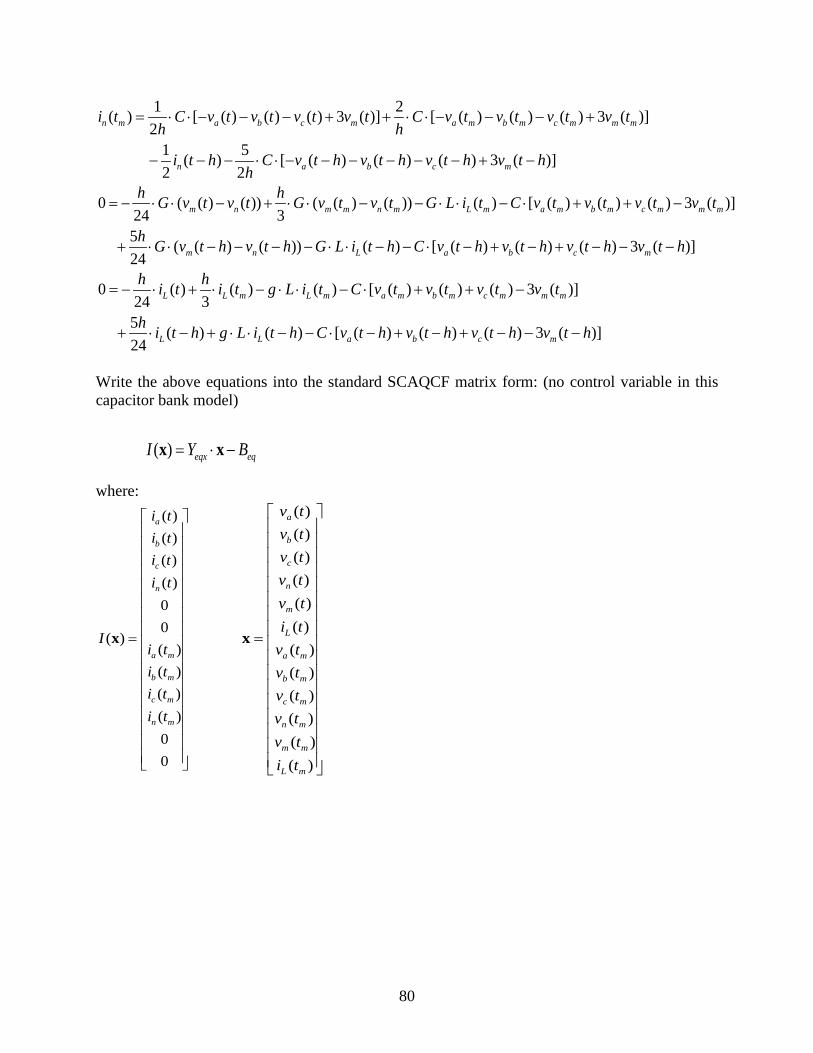
1 2( ) [ ( ) ( ) ( ) 3 ( )] [ ( ) ( ) ( ) 3 ( )]2

1 5 ( ) [ ( ) ( ) ( ) 3 ( )]2 2

n m a b c m a m b m c m m m

n a b c m

i t C v t v t v t v t C v t v t v t v th h


= ⋅ ⋅ − − − + + ⋅ ⋅ − − − +

− − − ⋅ ⋅ − − − − − − + −

0 ( ( ) ( )) ( ( ) ( )) ( ) [ ( ) ( ) ( ) 3 ( )]24 35 ( ( ) ( )) ( ) [ ( ) ( ) ( ) 3 ( )]24

m n m m n m L m a m b m c m m m

m n L a b c m

h hG v t v t G v t v t G L i t C v t v t v t v t


= − ⋅ ⋅ − + ⋅ ⋅ − − ⋅ ⋅ − ⋅ + + −

+ ⋅ ⋅ − − − − ⋅ ⋅ − − ⋅ − + − + − − −

0 ( ) ( ) ( ) [ ( ) ( ) ( ) 3 ( )]24 35 ( ) ( ) [ ( ) ( ) ( ) 3 ( )]24

L L m L m a m b m c m m m

L L a b c m



= − ⋅ + ⋅ − ⋅ ⋅ − ⋅ + + −

+ ⋅ − + ⋅ ⋅ − − ⋅ − + − + − − −

Write the above equations into the standard SCAQCF matrix form: (no control variable in this capacitor bank model)

( ) eqx eqI Y B= ⋅ −x x

where: ( )( )( )( )00

( )( )( )( )( )00

a

b

c

n

a m

b m

c m

n m

i ti ti ti t

Ii ti ti ti t

=

x

( )( )( )( )( )( )( )( )( )( )( )( )

a

b

c

n

m

L

a m

b m

c m

n m

m m

L m

v tv tv tv tv ti t

v tv tv tv tv ti t

=

x

80

12 12 24 240 0 0 0 0 0 0 0

12 12 24 240 0 0 0 0 0 0 0

12 12 24 240 0 0 0 0 0 0 0

12 12 12 36 24 24 24 720 0 0 0

2 23 0 0 0 06 6 3 3

20 3 0 0 0 0 06 3

20 0 0 0 0 0 02 2

eqx

C C C Ch h h h

C C C Ch h h h

C C C Ch h h h



h hC C C C g LY

C C Ch h h

− −

− −

− −

− − − −

⋅ ⋅ ⋅ ⋅− − − − + − ⋅ −

− − − − ⋅=

−2 0

2 20 0 0 0 0 0 0 02 2

2 20 0 0 0 0 0 0 02 2

3 2 2 2 60 0 0 02 2 2 2

0 0 0 0 324 24 3 3

0 0 0 0 0 0 324 3

Ch

C C C Ch h h h

C C C Ch h h h



h hC C C C g L

− − − − −

− − − − − − ⋅ ⋅ ⋅ ⋅

− − − − − + − ⋅ − − − − − ⋅

81

123 ( ) [ ( ) ( )]

123 ( ) [ ( ) ( )]

123 ( ) [ ( ) ( )]

123 ( ) [ ( ) ( ) ( ) 3 ( )]

( ( ) ( )) ( ) [ ( )6

a a m

b b m

c c m

n a b c m

m n L a

eq





h G v t h v t h G L i t h C v t h

B

− − − ⋅ ⋅ − − −

− − − ⋅ ⋅ − − −

− − − ⋅ ⋅ − − −

− − − ⋅ ⋅ − − − − − − + −

− ⋅ ⋅ − − − + ⋅ ⋅ − + ⋅ −

=

( ) ( ) 3 ( )]

( ) ( ) [ ( ) ( ) ( ) 3 ( )]6

1 5( ) [ ( ) ( )]2 21 5( ) [ ( ) ( )]2 2

1 5( ) [ ( ) ( )]2 21 5( )2

b c m

L L a b c m

a a m

b b m

c c m

n

v t h v t h v t h





i t h

+ − + − − −

− ⋅ − − ⋅ ⋅ − + ⋅ − + − + − − −

− − + ⋅ ⋅ − − −

− − + ⋅ ⋅ − − −

− − + ⋅ ⋅ − − −

− − + [ ( ) ( ) ( ) 3 ( )]2

5 ( ( ) ( )) ( ) [ ( ) ( ) ( ) 3 ( )]24

5 ( ) ( ) [ ( ) ( ) ( ) 3 ( )]24

a b c m

m n L a b c m

L L a b c m

C v t h v t h v t h v t hh



⋅ ⋅ − − − − − − + −

− ⋅ ⋅ − − − + ⋅ ⋅ − + ⋅ − + − + − − ⋅ −

− ⋅ − − ⋅ ⋅ − + ⋅ − + − + − − −

The input matrices of the capacitor bank SCAQCF device model for the setting-less protection algorithm are shown below:

TerminalNodeName CAPBANK_A CAPBANK_B CAPBANK_C CAPBANK_N -1

Xscale 0, 11500 1, 11500 2, 11500 3, 11500 4, 11500 5, 80 6, 11500

82

7, 11500 8, 11500 9, 11500 10, 11500 11, 80 -1

Iscale 0, 230 1, 230 2, 230 3, 230 4, 1 5, 1 6, 230 7, 230 8, 230 9, 230 10, 1 11, 1 -1

Yeqx 0, 0, 0.192 0, 4, -0.192 0, 6, -0.384 0, 10, 0.384 1, 1, 0.192 1, 4, -0.192 1, 7, -0.384 1, 10, 0.384 2, 2, 0.192 2, 4, -0.192 2, 8, -0.384 2, 10, 0.384 3, 0, -0.192 3, 1, -0.192 3, 2, -0.192 3, 4, 0.576 3, 6, 0.384 3, 7, 0.384 3, 8, 0.384 3, 10, -1.152 4, 0, -0.0000048 4, 1, -0.0000048 4, 2, -0.0000048 4, 3, -0.0000001667 4, 4, 0.0000145667

83

4, 9, -0.0000006667 4, 10, 0.0000006667 5, 0, -0.0000048 5, 1, -0.0000048 5, 2, -0.0000048 5, 4, 0.0000144 5, 5, 0.00001667 5, 11, 0.00006667 6, 0, 0.024 6, 4, -0.024 6, 6, 0.096 6, 10, -0.096 7, 1, 0.024 7, 4, -0.024 7, 7, 0.096 7, 10, -0.096 8, 2, 0.024 8, 4, -0.024 8, 8, 0.096 8, 10, -0.096 9, 0, -0.024 9, 1, -0.024 9, 2, -0.024 9, 4, 0.072 9, 6, -0.096 9, 7, -0.096 9, 8, -0.096 9, 10, 0.288 10, 3, 0.0000000416 10, 4, -0.0000000416 10, 6, -0.0000048 10, 7, -0.0000048 10, 8, -0.0000048 10, 9, -0.0000003333 10, 10, 0.0000147333 11, 5, -0.00000416 11, 6, -0.0000048 11, 7, -0.0000048 11, 8, -0.0000048 11, 10, 0.0000144 11, 11, 0.00003333 -1

Feqx -1

Neqx 0, 0, 0.192

84

0, 4, -0.192 1, 1, 0.192 1, 4, -0.192 2, 2, 0.192 2, 4, -0.192 3, 0, -0.192 3, 1, -0.192 3, 2, -0.192 3, 4, 0.576 4, 0, 0.0000048 4, 1, 0.0000048 4, 2, 0.0000048 4, 3, -0.0000001667 4, 4, -0.000014233 5, 0, 0.0000048 5, 1, 0.0000048 5, 2, 0.0000048 5, 4, -0.0000144 5, 5, 0.00001667 6, 0, -0.12 6, 4, 0.12 7, 1, -0.12 7, 4, 0.12 8, 2, -0.12 8, 4, 0.12 9, 0, 0.12 9, 1, 0.12 9, 2, 0.12 9, 4, -0.36 10, 0, 0.0000048 10, 1, 0.0000048 10, 2, 0.0000048 10, 3, -0.000000208 10, 4, -0.000014192 11, 0, 0.0000048 11, 1, 0.0000048 11, 2, 0.0000048 11, 4, -0.0000144 11, 5, 0.000000208 -1

Meq 0, 0, 1.0 1, 1, 1.0 2, 2, 1.0 3, 3, 1.0 6, 0, -0.5 7, 1, -0.5

85

8, 2, -0.5 9, 3, -0.5 -1

Keq

-1

C4. Three Phase Capacitor Bank SCAQCF Measurement Model

More specifically, for capacitor bank, the actual measurements are: Three currents at time t (phase A, phase B, and phase C); Three voltages at time t (phase A-G, phase B-G, phase C-G); Three bottom currents at time t (bottom phase A, bottom phase B, and bottom phase C); One neutral voltage at time t (phase N-G); Three currents at time tm=t-h/2 (phase A, phase B, and phase C); Three voltages at time tm=t-h/2 (phase A-G, phase B-G, phase C-G); Three bottom currents at time tm=t-h/2 (bottom phase A, bottom phase B, and bottom phase C); One neutral voltage at time tm=t-h/2 (phase N-G); The virtual measurements are: Two measurements with zero value at the left side of the equations at time t; Two measurements with zero value at the left side of the equations at time tm=t-h/2; The measurement channel list: MeasurementType, 16 MeasStdDev, 1150 MeasTerminal, 0, 3 MeasurementEnd MeasurementType, 17 MeasStdDev, 2 MeasTerminal, 0 MeasurementEnd MeasurementType, 17 MeasStdDev, 2 MeasTerminal, 1 MeasurementEnd MeasurementType, 17 MeasStdDev, 2 MeasTerminal, 2 MeasurementEnd MeasurementType, 16 MeasStdDev, 1150 MeasTerminal, 1, 3 MeasurementEnd MeasurementType, 16

86

MeasStdDev, 1150 MeasTerminal, 2, 3 MeasurementEnd MeasurementType, 16 MeasStdDev, 1150 MeasTerminal, 3 MeasurementEnd MeasurementType, 17 MeasStdDev, 2 MeasTerminal, 0 MeasurementEnd MeasurementType, 17 MeasStdDev, 2 MeasTerminal, 1 MeasurementEnd MeasurementType, 17 MeasStdDev, 2 MeasTerminal, 2 MeasurementEnd MeasurementType, 24 MeasStdDev, 0.0010000 MeasTerminal, 4 MeasurementEnd MeasurementType, 24 MeasStdDev, 0.0010000 MeasTerminal, 5 MeasurementEnd Based on the device model and the measurement channel list, the equations for the measurement model are given below: At time t ,

( ) ( ) ( )an a nv t v t v t= −

( ) ( ) ( )bn b nv t v t v t= −

( ) ( ) ( )cn c nv t v t v t= −

( ) ( )nn nv t v t= 4 8 4( ) [ ( ) ( )] [ ( ) ( )] ( ) [ ( ) ( )]a a n a m n m a a ni t C v t v t C v t v t i t h C v t h v t hh h h

= ⋅ ⋅ − − ⋅ ⋅ − + − + ⋅ ⋅ − − −

4 8 4( ) [ ( ) ( )] [ ( ) ( )] ( ) [ ( ) ( )]b b n b m n m b b ni t C v t v t C v t v t i t h C v t h v t hh h h

= ⋅ ⋅ − − ⋅ ⋅ − + − + ⋅ ⋅ − − − 4 8 4( ) [ ( ) ( )] [ ( ) ( )] ( ) [ ( ) ( )]c c n c m n m c c ni t C v t v t C v t v t i t h C v t h v t hh h h

= ⋅ ⋅ − − ⋅ ⋅ − + − + ⋅ ⋅ − − −

87

4 8 4( ) [ ( ) ( )] [ ( ) ( )] ( ) [ ( ) ( )]am a n a m n m a a ni t C v t v t C v t v t i t h C v t h v t hh h h

= ⋅ ⋅ − − ⋅ ⋅ − + − + ⋅ ⋅ − − −

4 8 4( ) [ ( ) ( )] [ ( ) ( )] ( ) [ ( ) ( )]bm b n b m n m b b ni t C v t v t C v t v t i t h C v t h v t hh h h

= ⋅ ⋅ − − ⋅ ⋅ − + − + ⋅ ⋅ − − − 4 8 4( ) [ ( ) ( )] [ ( ) ( )] ( ) [ ( ) ( )]cm c n c m n m c c ni t C v t v t C v t v t i t h C v t h v t hh h h

= ⋅ ⋅ − − ⋅ ⋅ − + − + ⋅ ⋅ − − −

0 ( )nv t= 20 ( ) ( ) ( ) [ ( ) ( ) ( ) 3 ( )]

6 3

( ) ( ) [ ( ) ( ) ( ) 3 ( )]6

n n m L a b c n

n L a b c n

h hG v t G v t G L i t C v t v t v t v t

h G v t h G L i t h C v t h v t h v t h v t h

= ⋅ ⋅ + ⋅ ⋅ − ⋅ ⋅ − ⋅ + + −

+ ⋅ ⋅ − + ⋅ ⋅ − − ⋅ − + − + − − −

20 ( ) ( ) ( ) [ ( ) ( ) ( ) 3 ( )]6 3

( ) ( ) [ ( ) ( ) ( ) 3 ( )]6

L L m L a b c n

L L a b c n



= ⋅ + ⋅ − ⋅ ⋅ − ⋅ + + −

+ ⋅ − + ⋅ ⋅ − − ⋅ − + − + − − −

At time mt ,

( ) ( ) ( )an m a m n mv t v t v t= −

( ) ( ) ( )bn m b m n mv t v t v t= −

( ) ( ) ( )cn m c m n mv t v t v t= −

( ) ( )nn m n mv t v t= 1 2 1 5( ) [ ( ) ( )] [ ( ) ( )] ( ) [ ( ) ( )]

2 2 2a m a n a m n m a a ni t C v t v t C v t v t i t h C v t h v t hh h h

= ⋅ ⋅ − + ⋅ ⋅ − − − − ⋅ ⋅ − − −

1 2 1 5( ) [ ( ) ( )] [ ( ) ( )] ( ) [ ( ) ( )]2 2 2b m b n b m n m b b ni t C v t v t C v t v t i t h C v t h v t h

h h h= ⋅ ⋅ − + ⋅ ⋅ − − − − ⋅ ⋅ − − −

1 2 1 5( ) [ ( ) ( )] [ ( ) ( )] ( ) [ ( ) ( )]2 2 2c m c n c m n m c c ni t C v t v t C v t v t i t h C v t h v t h

h h h= ⋅ ⋅ − + ⋅ ⋅ − − − − ⋅ ⋅ − − −

1 2 1 5( ) [ ( ) ( )] [ ( ) ( )] ( ) [ ( ) ( )]2 2 2am m a n a m n m a a ni t C v t v t C v t v t i t h C v t h v t h

h h h= ⋅ ⋅ − + ⋅ ⋅ − − − − ⋅ ⋅ − − −

1 2 1 5( ) [ ( ) ( )] [ ( ) ( )] ( ) [ ( ) ( )]2 2 2bm m b n b m n m b b ni t C v t v t C v t v t i t h C v t h v t h

h h h= ⋅ ⋅ − + ⋅ ⋅ − − − − ⋅ ⋅ − − −

1 2 1 5( ) [ ( ) ( )] [ ( ) ( )] ( ) [ ( ) ( )]2 2 2cm m c n c m n m c c ni t C v t v t C v t v t i t h C v t h v t h

h h h= ⋅ ⋅ − + ⋅ ⋅ − − − − ⋅ ⋅ − − −

0 ( )n mv t=

0 ( ) ( ) ( ) [ ( ) ( ) ( ) 3 ( )]24 35 ( ) ( ) [ ( ) ( ) ( ) 3 ( )]24

n n m L a b c n

n L a b c n

h hG v t G v t G L i t C v t v t v t v t

h G v t h G L i t h C v t h v t h v t h v t h

= − ⋅ ⋅ + ⋅ ⋅ − ⋅ ⋅ − ⋅ + + −

+ ⋅ ⋅ − + ⋅ ⋅ − − ⋅ − + − + − − −

88

0 ( ) ( ) ( ) [ ( ) ( ) ( ) 3 ( )]24 35 ( ) ( ) [ ( ) ( ) ( ) 3 ( )]24

L L m L a b c n

L L a b c n



= − ⋅ + ⋅ − ⋅ ⋅ − ⋅ + + −

+ ⋅ − + ⋅ ⋅ − − ⋅ − + − + − − −

It is very easy to write the above equations in the standard SCAQCF format:

, , , , , , ,( , ) ( ) ( ) ( )T i T i T im x m x m u m u m xu m x m u m mY F Y F F N t h N t h M I t h K

= + + + + + − + − + − +

y x u x x x u u u x u x u

89

where:

,

1 0 0 1 0 0 0 0 0 0 0 00 1 0 1 0 0 0 0 0 0 0 00 0 1 1 0 0 0 0 0 0 0 00 0 0 1 0 0 0 0 0 1 0 0

4 4 8 80 0 0 0 0 0 0 0

4 4 8 80 0 0 0 0 0 0 0

4 4 8 80 0 0 0 0 0 0 0

4 4 8 80 0 0 0 0 0 0 0

4 4 8 80 0 0 0 0 0 0 0

4 4 8 80 0 0 0 0 0 0 0

0 0 0 1 0 0 0 0 0 1 0 0

m x

C C C Ch h h h

C C C Ch h h h

C C C Ch h h h

C C C Ch h h h

C C C Ch h h h

C C C Ch h h h

Y

−−−

− −

− −

− −

− −

− −

− −

=

2 23 0 0 0 06 6 3 3

20 3 0 0 0 0 06 3

0 0 0 0 0 0 1 0 0 1 0 00 0 0 0 0 0 0 1 0 1 0 00 0 0 0 0 0 0 0 1 1 0 00 0 0 0 0 0 0 0 0 1 0 0

2 20 0 0 0 0 0 0 02 2

2 20 0 0 0 0 0 0 02 2

2 20 0 0 0 0 0 0 02 2

2 20 0 0 0 0 0 0 02 2

0


h hC C C C g L

C C C Ch h h h

C C C Ch h h h

C C C Ch h h h

C C C Ch h h h

⋅ ⋅ ⋅ ⋅− − − − + − ⋅ −

− − − − ⋅

−−−

− −

− −

− −

− −

2 20 0 0 0 0 0 02 2

2 20 0 0 0 0 0 0 02 2

0 0 0 0 0 0 0 0 0 1 0 0

0 0 0 0 324 24 3 3

0 0 0 0 0 0 324 3

C C C Ch h h h

C C C Ch h h h


h hC C C C g L

− − − −

⋅ ⋅ ⋅ ⋅ − − − − − + − ⋅ − − − − − ⋅

90

,

0 0 0 0 0 00 0 0 0 0 00 0 0 0 0 00 0 0 0 0 0

4 40 0 0 0

4 40 0 0 0

4 40 0 0 0

4 40 0 0 0

4 40 0 0 0

4 40 0 0 0

0 0 0 0 0 0

36 6

0 36

0 0 0 0 0 00 0 0 0 0 00 0 0 0 0 00 0 0 0 0 05 50 0 0 02 2

5 50 0 0 02 2

5 50 0 0 02 2

52

m x

C Ch h

C Ch h

C Ch h

C Ch h

C Ch h

C Ch h

h G h GC C C C G L

hC C C C g LN

C Ch h

C Ch h

C Ch h

Ch

−

−

−

−

−

−

⋅ ⋅− + ⋅

− − ⋅=

−

−

−

−50 0 0 02

5 50 0 0 02 2

5 50 0 0 02 2

0 0 0 0 0 05 5 3

24 2450 324

Ch

C Ch h

C Ch h

h G h GC C C C G L

hC C C C g L

− −

⋅ ⋅ − − ⋅ − − ⋅

91

0 0 0 00 0 0 00 0 0 00 0 0 01 0 0 00 1 0 00 0 1 01 0 0 00 1 0 00 0 1 00 0 0 00 0 0 00 0 0 00 0 0 00 0 0 00 0 0 00 0 0 01 0 0 02

10 0 02

10 0 02

1 0 0 02

10 0 02

10 0 02

0 0 0 00 0 0 00 0 0 0

mM

= −

−

−− − −

92

Appendix D: Time Domain SCAQCF Model – Single Section Transmission Line Protection

This Appendix presents the derivation of the time domain model of a transmission line in the SCAQCF syntax. The model is first presented with what we call the compact form, which is the familiar standard notation model. We subsequently quadratize the model and then the quadratic model is integrated to provide the SCAQCF device model. A typical measurement channel list is also presented to show the procedure of creating the SCAQCF measurement model.

D1. Three Phase Transmission Line Compact Model Figure D1 gives the circuit model of the three phase four wire transmission line.

1( )ai t1( )bi t1( )ci t1( )ni t

1( )av t1( )bv t1( )cv t1( )nv t

2 ( )ai t2 ( )bi t2 ( )ci t

2 ( )ni t

2 ( )av t2 ( )bv t2 ( )cv t2 ( )nv t

Matrix R Matrix L


Matrix C Matrix C

( )Lai t( )

Lbi t( )

Lci t( )

Lni t

Figure D.1: The Three Phase Transmission Line Circuit Model

The compact transmission line model is derived from this circuit and it is given with the following equations:

11

( ) ( )( ) ( ) LL

dv t di ti t C i t GLdt dt

= + +

22

( ) ( )( ) ( ) LL

dv t di ti t C i t GLdt dt

= − −

1 2( ) ( )0 ( ) ( ) ( ( ) )L L

Ldi t di tv t v t R i t GL L

dt dt= − + + + +

In compact matrix form, the model is:

( ) ( )( )( ) ( )0 L L


= ⋅ + ⋅

93

where:

1 1

1 1

1 1

1 1

2 2

2 2

2 2

2 2

( ) ( )( ) ( )( ) ( )( ) ( )

( ) , ( )( ) ( )( ) ( )( ) ( )( ) ( )

a a

b b

c c

n n

a a

b b

c c

n n

i t v ti t v ti t v ti t v t

i t v ti t v ti t v ti t v ti t v t

= =

4 4

4 4

4 4 4 4

0 0 00 0 0

0 0

I C G LA I B C G L

I I R R G L L

×

×

× ×

⋅ = − = − ⋅ − ⋅ ⋅ +

, , , R L C G are the resistance, inductance, capacitance and stabilizing conductance matrices of the transmission line (as shown in the above figure).

D2. Three Phase Transmission Line Quadratized Model All the terms in the three phase transmission line compact model are linear and quadratic terms. Therefore the quadratized model is identical to the compact model. In compact matrix form, the model is:

( ) ( )( )( ) ( )0 L L


= ⋅ + ⋅

where:

1 1

1 1

1 1

1 1

2 2

2 2

2 2

2 2

( ) ( )( ) ( )( ) ( )( ) ( )

( ) , ( )( ) ( )( ) ( )( ) ( )( ) ( )

a a

b b

c c

n n

a a

b b

c c

n n

i t v ti t v ti t v ti t v t

i t v ti t v ti t v ti t v ti t v t

= =

4 4

4 4

4 4 4 4

0 0 00 0 0

0 0

I C G LA I B C G L

I I R R G L L

×

×

× ×

⋅ = − = − ⋅ − ⋅ ⋅ +

94

D3. Three Phase Transmission Line SCAQCF Device Model The state and control algebraic quadratic companion form (SCAQCF) device model is derived after quadratic integration of the quadratized model with a time step h. The result is:

( ) eqx eqI Y B= ⋅ −x x


where: ( )0000

( )( )0000

m

i t

Ii t

=

x

( )( )

( )( )

L

m

L m

v ti tv ti t

=

x

𝑖𝑖(𝑜𝑜) = [𝑖𝑖𝑚𝑚1(𝑜𝑜), 𝑖𝑖𝑏𝑏1(𝑜𝑜), 𝑖𝑖𝑐𝑐1(𝑜𝑜), 𝑖𝑖𝑛𝑛1(𝑜𝑜), 𝑖𝑖𝑚𝑚2(𝑜𝑜), 𝑖𝑖𝑏𝑏2(𝑜𝑜), 𝑖𝑖𝑐𝑐2(𝑜𝑜), 𝑖𝑖𝑛𝑛2(𝑜𝑜)] 𝑖𝑖(𝑜𝑜𝑚𝑚) = [𝑖𝑖𝑚𝑚1(𝑜𝑜𝑚𝑚), 𝑖𝑖𝑏𝑏1(𝑜𝑜𝑚𝑚), 𝑖𝑖𝑐𝑐1(𝑜𝑜𝑚𝑚), 𝑖𝑖𝑛𝑛1(𝑜𝑜𝑚𝑚), 𝑖𝑖𝑚𝑚2(𝑜𝑜𝑚𝑚), 𝑖𝑖𝑏𝑏2(𝑜𝑜𝑚𝑚), 𝑖𝑖𝑐𝑐2(𝑜𝑜𝑚𝑚), 𝑖𝑖𝑛𝑛2(𝑜𝑜𝑚𝑚)]

𝑣𝑣(𝑜𝑜) = [𝑣𝑣𝑚𝑚1(𝑜𝑜), 𝑣𝑣𝑏𝑏1(𝑜𝑜), 𝑣𝑣𝑐𝑐1(𝑜𝑜), 𝑣𝑣𝑛𝑛1(𝑜𝑜), 𝑣𝑣𝑚𝑚2(𝑜𝑜), 𝑣𝑣𝑏𝑏2(𝑜𝑜), 𝑣𝑣𝑐𝑐2(𝑜𝑜), 𝑣𝑣𝑛𝑛2(𝑜𝑜)] 𝑣𝑣(𝑜𝑜𝑚𝑚) = [𝑣𝑣𝑚𝑚1(𝑜𝑜𝑚𝑚), 𝑣𝑣𝑏𝑏1(𝑜𝑜𝑚𝑚),𝑣𝑣𝑐𝑐1(𝑜𝑜𝑚𝑚),𝑣𝑣𝑛𝑛1(𝑜𝑜𝑚𝑚), 𝑣𝑣𝑚𝑚2(𝑜𝑜𝑚𝑚),𝑣𝑣𝑏𝑏2(𝑜𝑜𝑚𝑚), 𝑣𝑣𝑐𝑐2(𝑜𝑜𝑚𝑚), 𝑣𝑣𝑛𝑛2(𝑜𝑜𝑚𝑚)]

𝑖𝑖𝐿𝐿(𝑜𝑜) = [𝑖𝑖𝑚𝑚𝐿𝐿(𝑜𝑜), 𝑖𝑖𝑏𝑏𝐿𝐿(𝑜𝑜), 𝑖𝑖𝑐𝑐𝐿𝐿(𝑜𝑜), 𝑖𝑖𝑛𝑛𝐿𝐿(𝑜𝑜)] 𝑖𝑖𝐿𝐿(𝑜𝑜𝑚𝑚) = [𝑖𝑖𝑚𝑚𝐿𝐿(𝑜𝑜𝑚𝑚), 𝑖𝑖𝑏𝑏𝐿𝐿(𝑜𝑜𝑚𝑚), 𝑖𝑖𝑐𝑐𝐿𝐿(𝑜𝑜𝑚𝑚), 𝑖𝑖𝑛𝑛𝐿𝐿(𝑜𝑜𝑚𝑚)]

4

4

4 4

4

4

4 4

4 4 8 80 0

4 4 8 80 0

4 8( ) 0 0 ( )

1 1 2 20 02 2

1 1 2 20 02 2

1 20 0 ( ) ( )2

eqx

C I GL C GLh h h h

C I GL C GLh h h h


C GL C I GLh h h h

C GL C I GLh h h h


+ − − − − − − + + − + = +

− − − + − + +

95

4

4

4 4

4

4

4 4

8 40

8 40

4 ( )

5 1 502 2 2

5 1 502 2 2

1 1 1 5 ( )2 2 2 2

eqx

C I GLh h

C I GLh h

I I R RGL LhN

C I GLh h

C I GLh h

I I R RGL Lh

− − + − − + = − +

− − − + +

4

4

4

4

0 0

0 0

0 0 0

1 0 02

10 02

0 0 0

eq

I

I

MI

I

= −

−

The input matrices of the capacitor bank SCAQCF device model for the setting-less protection algorithm are shown below: TerminalNodeName YJLINE1_A YJLINE1_B YJLINE1_C YJLINE1_N YJLINE2_A YJLINE2_B YJLINE2_C YJLINE2_N -1 Xscale 0,115000.00 1,115000.00 2,115000.00 3,115000.00 4,115000.00 5,115000.00 6,115000.00 7,115000.00 8,500.00 9,500.00 10,500.00

96

11,500.00 12,115000.00 13,115000.00 14,115000.00 15,115000.00 16,115000.00 17,115000.00 18,115000.00 19,115000.00 20,500.00 21,500.00 22,500.00 23,500.00 -1 Iscale 0,500.00 1,500.00 2,500.00 3,500.00 4,500.00 5,500.00 6,500.00 7,500.00 8,115000.00 9,115000.00 10,115000.00 11,115000.00 12,500.00 13,500.00 14,500.00 15,500.00 16,500.00 17,500.00 18,500.00 19,500.00 20,115000.00 21,115000.00 22,115000.00 23,115000.00 -1 Yeqx 0,0,0.0059165000 0,1,-0.0014640000 0,2,-0.0007320000 0,3,-0.0011400000 0,8,1.6666666667 0,9,0.3422733078 0,10,0.3014048531 0,11,0.3346104725 0,12,-0.0118080000 0,13,0.0029280000 0,14,0.0014640000 0,15,0.0022800000

97

0,20,-1.3333333333 0,21,-0.6845466156 0,22,-0.6028097063 0,23,-0.6692209451 1,0,-0.0014640000 1,1,0.0060845000

23,22,0.0335621593 23,23,0.1158563363 -1 Feqx -1 Neqx 0,0,0.0058915000 0,1,-0.0014640000 0,2,-0.0007320000

23,10,-0.0334556568 23,11,-0.1077480413 -1 Meq 0,0,1.0000000000 1,1,1.0000000000 2,2,1.0000000000 3,3,1.0000000000 4,4,1.0000000000 5,5,1.0000000000 6,6,1.0000000000 7,7,1.0000000000 12,0,-0.5000000000 13,1,-0.5000000000 14,2,-0.5000000000 15,3,-0.5000000000 16,4,-0.5000000000 17,5,-0.5000000000 18,6,-0.5000000000 19,7,-0.5000000000 -1 Keq -1

98

D4. Three Phase Transmission Line SCAQCF Measurement Model

Specifically, for single section transmission line, the actual measurements are: Three currents at left side at time t (phase A_1, phase B_1, and phase C_1); Three currents at right side at time t (phase A_2, phase B_2, and phase C_2); Three voltages at left side time t (phase A-G_1, phase B-G_1, phase C-G_1); Three voltages at left side time t (phase A-G_2, phase B-G_2, phase C-G_2); Three currents at left side at time tm (phase A_1, phase B_1, and phase C_1); Three currents at right side at time tm (phase A_2, phase B_2, and phase C_2); Three voltages at left side time tm (phase A-G_1, phase B-G_1, phase C-G_1); Three voltages at left side time tm (phase A-G_2, phase B-G_2, phase C-G_2); The virtual measurements are: Four measurements with zero value at from KVL equation at time t; Two measurements with zero value at from KVL equation at time tm=t-h/2; The measurements definition is shown as follows: MeasurementType, 16 MeasStdDev, 1080 MeasTerminal, 0, 3 MeasurementEnd MeasurementType, 16 MeasStdDev, 1080 MeasTerminal, 1, 3 MeasurementEnd MeasurementType, 16 MeasStdDev, 1080 MeasTerminal, 2, 3 MeasurementEnd MeasurementType, 16 MeasStdDev, 1080 MeasTerminal, 4, 7 MeasurementEnd MeasurementType, 16 MeasStdDev, 1080 MeasTerminal, 5, 7 MeasurementEnd MeasurementType, 16 MeasStdDev, 1080 MeasTerminal, 6, 7 MeasurementEnd MeasurementType, 17 MeasStdDev, 5.0 MeasTerminal, 0 MeasurementEnd MeasurementType, 17 MeasStdDev, 5.0 MeasTerminal, 1 MeasurementEnd

99

MeasurementType, 17 MeasStdDev, 5.0 MeasTerminal, 2 MeasurementEnd MeasurementType, 17 MeasStdDev, 5.0 MeasTerminal, 4 MeasurementEnd MeasurementType, 17 MeasStdDev, 5.0 MeasTerminal, 5 MeasurementEnd MeasurementType, 17 MeasStdDev, 5.0 MeasTerminal, 6 MeasurementEnd MeasurementType, 24 MeasStdDev, 108 MeasTerminal, 8 MeasurementEnd MeasurementType, 24 MeasStdDev, 108 MeasTerminal, 9 MeasurementEnd MeasurementType, 24 MeasStdDev, 108 MeasTerminal, 10 MeasurementEnd MeasurementType, 24 MeasStdDev, 108 MeasTerminal, 11 MeasurementEnd Based on the device model and the measurement channel list, the equations for the measurement model are given below:


= + + + + + − + − + − +


100

where:

4

4

4 4

4

4

4 4

0 0 0 0 0

0 0 0 0 0

4 4 8 80 0

4 4 8 80 0

4 8( ) 0 0 ( )

0 0 0 0 0

0 0 0 0 0

1 1 2 20 02 2

1 1 2 20 02 2

1 20 0 ( ) ( )2

mx

K

K

C I GL C GLh h h h

C I GL C GLh h h h


K

K

C GL C I GLh h h h

C GL C I GLh h h h


+ − − − − −

− + + − += + − − −

+ − + +

1 0 0 10 1 0 10 0 1 10 0 0 1

K

− − = −

101

4

4

4 4

4

4

4 4

0 0 0

0 0 0

8 40

8 40

4 ( )

0 0 0

0 0 0

5 1 502 2 2

5 1 502 2 2

1 1 1 5 ( )2 2 2 2

m

C I GLh h

C I GLh h

I I R RGL LhN

C I GLh h

C I GLh h

I I R RGL Lh

− − +

− − + = − + −

− − + +

4

4

4

4

0 0 0

0 0 0

0 0

0 0

0 0 0

0 0 0

0 0 0

1 0 02

10 02

0 0 0

eq

I

I

M

I

I

= −

−

102

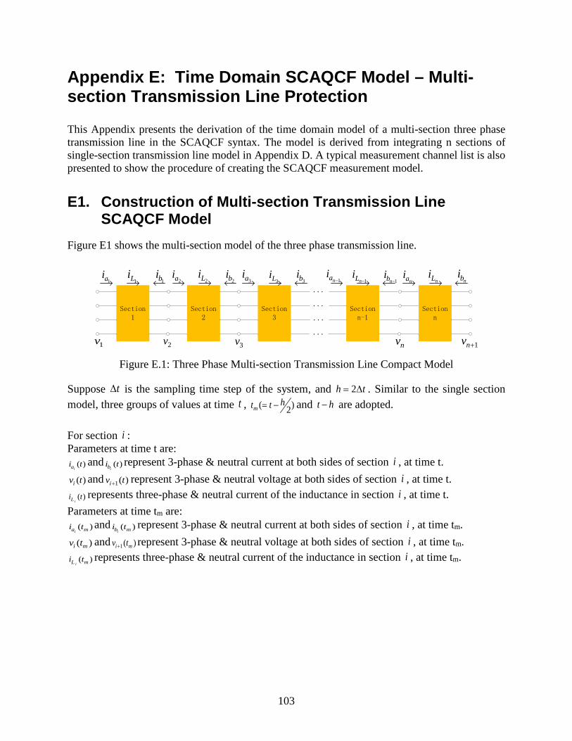
Appendix E: Time Domain SCAQCF Model – Multi-section Transmission Line Protection

This Appendix presents the derivation of the time domain model of a multi-section three phase transmission line in the SCAQCF syntax. The model is derived from integrating n sections of single-section transmission line model in Appendix D. A typical measurement channel list is also presented to show the procedure of creating the SCAQCF measurement model.

E1. Construction of Multi-section Transmission Line SCAQCF Model

Figure E1 shows the multi-section model of the three phase transmission line.

Section 1

Section 2

Section 3

...

...

...

Section n-1

Section n

1ai 1Li

1v

2ai 2Li1bi 3ai 3Li2bi 3bi 1nai − 1nLi − 1nbi − nai nLi nbi

2v 3v nv 1nv +

...

Figure E.1: Three Phase Multi-section Transmission Line Compact Model

Suppose t∆ is the sampling time step of the system, and 2h t= ∆ . Similar to the single section model, three groups of values at time t , ( )2m

ht t= − and t h− are adopted. For section i : Parameters at time t are:

( )iai t and ( )

ibi t represent 3-phase & neutral current at both sides of section i , at time t. ( )iv t and 1( )iv t+ represent 3-phase & neutral voltage at both sides of section i , at time t. ( )

iLi t represents three-phase & neutral current of the inductance in section i , at time t. Parameters at time tm are:

( )ia mi t and ( )

ib mi t represent 3-phase & neutral current at both sides of section i , at time tm. ( )i mv t and 1( )i mv t+ represent 3-phase & neutral voltage at both sides of section i , at time tm. ( )

iL mi t represents three-phase & neutral current of the inductance in section i , at time tm.

103

For each section, the formulation is similar to the single section model in Appendix D. For example, equations in section k are:

1

1

1

(1)( ) ( )(2)( ) ( )

( ) (3)0( ) ( ) (4)

( )( ) (5)( )0 (6)

kk

kk

k k

k k

k k

kk

eqa k

eqb k

L eq

a m k m eq

k mb m eq

L m eq

bi t v tbi t v t

i t bE F

i t v t bv ti t bi t b

+

+

= ⋅ − where:

(1) (2) (3) (4) (5) (6)k k k k k k k

Teq eq eq eq eq eq eqb b b b b b b =

and ( )keqb j is a 4-element vector, 1,2, ,6j = ;

2 1 3

( )( )( ) ( )

( ) 0

k

k k

k

ak

eq k b

L

i t hv t hb E F v t h E F i t h

i t h+

− −

= ⋅ ⋅ − + ⋅ ⋅ − −

also, 1

12 12 12 12 12 12 12 12

12 12 12 12 12 12 12 12

2 4 86 3

1 224 3 2

h hI I I Ih hE

h hI I I Ih h

−

× × × ×

× × × ×

− = =

−

1

26 3

24 3

h hA B AF

h hA A B

+ =

− + ,

26

524

hB AF

hB A

− =

− ,

12 12

3

12 12

6524

h IF

h I

×

×

=

4 4

4 4

4 4 4 4

0 0 00 0 0

0 0

I C G LA I B C G L

I I R R G L L

×

×

× ×

⋅ = − = − ⋅ − ⋅ ⋅ +

where R , L and C are the resistance, inductance and capacitance matrices of each section; G is the stabilizing conductance matrix of each section.

E2. Three Phase Multi-section Transmission Line SCAQCF Model

Divide 1E F⋅ as follows, with each : 4 4 ( , 1, 2,...,6)jkM j k× = : 11 12 13 14 15 16

21 22 23 24 25 26

31 32 33 34 35 361

41 42 43 44 45 46

51 52 53 54 55 56

61 62 63 64 65 66

M M M M M MM M M M M MM M M M M M

E FM M M M M MM M M M M MM M M M M M

⋅ =

104

Divide 2E F⋅ as follows, with each : 4 4 ( 1,2,...,6, 1, 2,3)jkP j k× = = : 11 12 13

21 22 23

31 32 332

41 42 43

51 52 53

61 62 63

P P PP P PP P P

E FP P PP P PP P P

⋅ =

Additionally,

12 12 12 12 12 1212 12

312 12

12 12 12 12 12 12

4 86

0.51 2 52 24

hI I I Ih hE FIhI I I

h h

× × ××

×× × ×

− − ⋅ = × =

Thus, for time t: Actual measurements:

1 1 1

1 1

11 1 12 2 13 14 1 15 2 16

11 1 12 2 13

( ) ( ) ( ) ( ) ( ) ( ) ( )

[ ( ) ( ) ( )] [ ( )]a L m m L m

L a

i t M v t M v t M i t M v t M v t M i t

P v t h P v t h P i t h i t h

= + + + + +

− − + − + − − − −

21 22 1 23 24 25 1 26

21 22 1 23

( ) ( ) ( ) ( ) ( ) ( ) ( )

[ ( ) ( ) ( )] [ ( )]n n n

n n

b n n L n m n m L m

n n L b


P v t h P v t h P i t h i t h+ +

+

= + + + + +

− − + − + − − − −

Virtual current measurements:

( )( )

( )

1 2

1 2

1 2

1 2

1

21 1 22 11 2 12 3 23 13

24 1 25 14 2 15 3 26 16

21 1 22 11 2 12 3 23 13

( ) ( ) 0

0 ( ) ( ) ( ) ( ) ( )

( ) ( ) ( ) ( ) ( )

[ ( ) ( ) ( ) ( ) ( )]

[ ( )

b a

L L

m m m L m L m

L L

b

i t i t

M v t M M v t M v t M i t M i t


P v t h P P v t h P v t h P i t h P i t h

i t h i

+ = ⇒

= + + + + +

+ + + + + +

− − + + − + − + − + −

− − − −2( )]a t h−

( )( )

( )

2 3

2 3

2 3

2 3

2

21 2 22 11 3 12 4 23 13

24 2 25 14 3 15 4 26 16

21 2 22 11 3 12 4 23 13

( ) ( ) 0

0 ( ) ( ) ( ) ( ) ( )

( ) ( ) ( ) ( ) ( )

[ ( ) ( ) ( ) ( ) ( )]

[ ( )

b a

L L

m m m L m L m

L L

b

i t i t




i t h i

+ = ⇒

= + + + + +

+ + + + + +

− − + + − + − + − + −

− − − −3( )]a t h−

( )( )

( )

1

1

1

1

21 1 22 11 12 1 23 13

24 1 25 14 15 1 26 16

21 1 22 11 12 1 23 13

( ) ( ) 0

0 ( ) ( ) ( ) ( ) ( )

( ) ( ) ( ) ( ) ( )

[ ( ) ( ) ( ) ( )

n n

n n

n n

n

b a

n n n L L

n m n m n m L m L m

n n n L L

i t i t



P v t h P P v t h P v t h P i t h P i

−

−

−

−

− +

− +

− +

+ = ⇒

= + + + + +

+ + + + + +

− − + + − + − + − +

1

( )]

[ ( ) ( )]n

n nb a

t h

i t h i t h−

−

− − − − −

Virtual voltage measurements: 1 1

1

31 1 32 2 33 34 1 35 2 36

31 1 32 2 33

0 ( ) ( ) ( ) ( ) ( ) ( )

[ ( ) ( ) ( )]L m m L m

L

M v t M v t M i t M v t M v t M i t

P v t h P v t h P i t h

= + + + + +

− − + − + −

2 2

2

31 2 32 3 33 34 2 35 3 36

31 2 32 3 33

0 ( ) ( ) ( ) ( ) ( ) ( )

[ ( ) ( ) ( )]L m m L m

L



= + + + + +

− − + − + −

105

31 32 1 33 34 35 1 36

31 32 1 33

0 ( ) ( ) ( ) ( ) ( ) ( )

[ ( ) ( ) ( )]n n

n

n n L n m n m L m

n n L


P v t h P v t h P i t h+ +

+

= + + + + +

− − + − + −

For time tm: Actual measurements:

1 1 1

1 1

41 1 42 2 43 44 1 45 2 46

41 1 42 2 43

( ) ( ) ( ) ( ) ( ) ( ) ( )

[ ( ) ( ) ( )] [0.5 ( )]a m L m m L m

L a


P v t h P v t h P i t h i t h

= + + + + +

− − + − + − − −

51 52 1 53 54 55 1 56

51 52 1 53

( ) ( ) ( ) ( ) ( ) ( ) ( )

[ ( ) ( ) ( )] [0.5 ( )]n n n

n n

b m n n L n m n m L m

n n L b


P v t h P v t h P i t h i t h+ +

+

= + + + + +

− − + − + − − − Virtual current measurements:

( )( )

( )

1 2

1 2

1 2

1 2

1

51 1 52 41 2 42 3 53 43

54 1 55 44 2 45 3 56 46

51 1 52 41 2 42 3 53 43

( ) ( ) 0

0 ( ) ( ) ( ) ( ) ( )

( ) ( ) ( ) ( ) ( )

[ ( ) ( ) ( ) ( ) ( )]

[0.5 (

b m a m

L L

m m m L m L m

L L

b

i t i t




i t

+ = ⇒

= + + + + +

+ + + + + +

− − + + − + − + − + −

− −2

) 0.5 ( )]ah i t h+ −

( )( )

( )

2 3

2 3

2 3

2 3

2

51 2 52 41 3 42 4 53 43

54 2 55 44 3 45 4 56 46

51 2 52 41 3 42 4 53 43

( ) ( ) 0

0 ( ) ( ) ( ) ( ) ( )

( ) ( ) ( ) ( ) ( )

[ ( ) ( ) ( ) ( ) ( )]

[0.5 (

b m a m

L L

m m m L m L m

L L

b

i t i t




i t

+ = ⇒

= + + + + +

+ + + + + +

− − + + − + − + − + −

− −3

) 0.5 ( )]ah i t h+ −

( )( )

( )

1

1

1

1

51 1 52 41 42 1 53 43

54 1 55 44 45 1 56 46

51 1 52 41 42 1 53 43

( ) ( ) 0

0 ( ) ( ) ( ) ( ) ( )

( ) ( ) ( ) ( ) ( )

[ ( ) ( ) ( ) ( )

n n

n n

n n

n

b m a m

n n n L L

n m n m n m L m L m

n n n L

i t i t



P v t h P P v t h P v t h P i t h P

−

−

−

−

− +

− +

− +

+ = ⇒

= + + + + +

+ + + + + +

− − + + − + − + − +

1

( )]

[0.5 ( ) 0.5 ( )]n

n n

L

b a

i t h

i t h i t h−

−

− − + −

106

Virtual voltage measurements: 1 1

1

61 1 62 2 63 64 1 65 2 66

61 1 62 2 63

0 ( ) ( ) ( ) ( ) ( ) ( )

[ ( ) ( ) ( )]L m m L m

L



= + + + + +

− − + − + −

2 2

2

61 2 62 3 63 64 2 65 3 66

61 2 62 3 63

0 ( ) ( ) ( ) ( ) ( ) ( )

[ ( ) ( ) ( )]L m m L m

L



= + + + + +

− − + − + −

61 62 1 63 64 65 1 66

61 62 1 63

0 ( ) ( ) ( ) ( ) ( ) ( )

[ ( ) ( ) ( )]n n

n

n n L n m n m L m

n n L


P v t h P v t h P i t h+ +

+

= + + + + +

− − + − + −

Write the above equations into the standard SCAQCF matrix form: (no control variable in this model)

( ) eqx eqI x Y x B= ⋅ − where:

[ ][ ]

[ ][ ]

1

1

( )

( )

0 0 0

0 0 0( )

( )

( )

0 0 0

0 0 0

n

n

a

b

T

T

a m

b m

T

T

i t

i t

I xi t

i t

=

[ ]

[ ]

1 2

1 2

1

1

2 3

1

1

2 3

( )( )

( ) ( ) ( )

( ) ( ) ( )

( )( )

( ) ( ) ( )

( ) ( ) ( )

n

n

nT

nT

L L L

m

n mT

m m n mT

L m L m L m

v tv t

v t v t v t

i t i t i tx

v tv t

v t v t v t

i t i t i t

+

+

=

11 12 13 14

21 22 23 24

31 32 33 34

41 42 43 44

eqx

Y Y Y YY Y Y Y

YY Y Y YY Y Y Y

=

( ) ( )

11 12

22 21

21 22 11 1211

21 22 11 12

12 21 22 11 4 4 4 4

0 0 0 0 00 0 0 0 0

0 0 0 00 0 0 0

0 0 0 0 n n

M MM M

M M M MY

M M M M

M M M M+ × +

+

= +

+

( ) ( )

14 15

25 24

24 25 14 1513

24 25 14 15

15 24 25 14 4 4 4 4

0 0 0 0 00 0 0 0 0

0 0 0 00 0 0 0

0 0 0 0 n n

M MM M

M M M MY

M M M M

M M M M+ × +

+

= +

+

( ) ( )

13

23

23 1312

23 13

23 13 4 4 4

0 0 0 00 0 0 0

0 0 00 0 0

0 0 0 n n

MM

M MY

M M

M M+ ×

=

( ) ( )

16

26

26 1614

26 16

26 16 4 4 4

0 0 0 00 0 0 0

0 0 00 0 0

0 0 0 n n

MM

M MY

M M

M M+ ×

=

107

( ) ( )

31 32

31 3221

32 31 4 4 4

0 0 00 0 0

0 0 0 n n

M MM M

Y

M M× +

=

( ) ( )

33

3322

33 4 4

0 0 00 0 0

0 0 0 n n

MM

Y

M×

=

( ) ( )

34 35

34 3523

35 34 4 4 4

0 0 00 0 0

0 0 0 n n

M MM M

Y

M M× +

=

( ) ( )

36

3624

36 4 4

0 0 00 0 0

0 0 0 n n

MM

Y

M×

=

( ) ( )

41 42

52 51

51 52 41 4231

51 52 41 42

42 51 52 41 4 4 4 4

0 0 0 0 00 0 0 0 0

0 0 0 00 0 0 0

0 0 0 0 n n

M MM M

M M M MY

M M M M

M M M M+ × +

+

= +

+

( ) ( )

44 45

55 54

54 55 44 4533

54 55 44 45

45 54 55 44 4 4 4 4

0 0 0 0 00 0 0 0 0

0 0 0 00 0 0 0

0 0 0 0 n n

M MM M

M M M MY

M M M M

M M M M+ × +

+

= +

+

( ) ( )

43

53

53 4332

53 43

53 43 4 4 4

0 0 0 00 0 0 0

0 0 00 0 0

0 0 0 n n

MM

M MY

M M

M M+ ×

=

( ) ( )

46

56

56 4634

56 46

56 46 4 4 4

0 0 0 00 0 0 0

0 0 00 0 0

0 0 0 n n

MM

M MY

M M

M M+ ×

=

( ) ( )

61 62

61 6241

62 61 4 4 4

0 0 00 0 0

0 0 0 n n

M MM M

Y

M M× +

=

( ) ( )

63

6342

63 4 4

0 0 00 0 0

0 0 0 n n

MM

Y

M×

=

( ) ( )

64 65

64 6543

65 64 4 4 4

0 0 00 0 0

0 0 0 n n

M MM M

Y

M M× +

=

( ) ( )

66

6644

66 4 4

0 0 00 0 0

0 0 0 n n

MM

Y

M×

=

and,

[ ] [ ][ ]

1

1 2

1

1

2 3

( )( )( ) ( )

( ) ( ) ( ) 0 0 0( ) ( ) ( ) 0 0 0

n

n

a

n bTeq eqx eq T

nT T

L L L

i t hv t hv t h i t h

B N Mv t h v t h v t h

i t h i t h i t h

+

−− − −

= − − − − − − − −

108

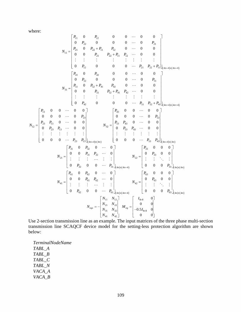
where:

( ) ( )

11 12

22 21

21 22 11 1211

21 22 11 12

12 21 22 11 4 4 4 4

0 0 0 0 00 0 0 0 0

0 0 0 00 0 0 0

0 0 0 0 n n

P PP P

P P P PN

P P P P

P P P P+ × +

+

= +

+

( ) ( )

41 42

52 51

51 52 41 4231

51 52 41 42

42 51 52 41 4 4 4 4

0 0 0 0 00 0 0 0 0

0 0 0 00 0 0 0

0 0 0 0 n n

P PP P

P P P PN

P P P P

P P P P+ × +

+

= +

+

( ) ( )

13

23

23 1312

23 13

23 13 4 4 4

0 0 0 00 0 0 0

0 0 00 0 0

0 0 0 n n

PP

P PN

P P

P P+ ×

=

( ) ( )

43

53

53 4332

53 43

53 43 4 4 4

0 0 0 00 0 0 0

0 0 00 0 0

0 0 0 n n

PP

P PN

P P

P P+ ×

=

( ) ( )

31 32

31 3221

32 31 4 4 4

0 0 00 0 0

0 0 0 n n

P PP P

N

P P× +

=

( ) ( )

33

3322

33 4 4

0 0 00 0 0

0 0 0 n n

PP

N

P×

=

( ) ( )

61 62

61 6241

62 61 4 4 4

0 0 00 0 0

0 0 0 n n

P PP P

N

P P× +

=

( ) ( )

63

6342

63 4 4

0 0 00 0 0

0 0 0 n n

PP

N

P×

=

11 12

21 22

31 32

41 42

eqx

N NN N

NN NN N

= −

8 8

8 8

00 0

0.5 00 0

eq

I

MI

×

×

= −

Use 2-section transmission line as an example. The input matrices of the three phase multi-section transmission line SCAQCF device model for the setting-less protection algorithm are shown below:

TerminalNodeName TABL_A TABL_B TABL_C TABL_N VACA_A VACA_B

109

VACA_C VACA_N -1 Xscale 0 , 500000 1 , 500000 2 , 500000 3 , 500000 4 , 500000 5 , 500000 6 , 500000 7 , 500000 8 , 500000 9 , 500000 10 , 500000 11 , 500000 12 , 4041 13 , 4041 14 , 4041 15 , 4041 16 , 4041 17 , 4041 18 , 4041 19 , 4041 20 , 500000 21 , 500000 22 , 500000 23 , 500000 24 , 500000 25 , 500000 26 , 500000 27 , 500000 28 , 500000 29 , 500000 30 , 500000 31 , 500000 32 , 4041 33 , 4041 34 , 4041 35 , 4041 36 , 4041 37 , 4041 38 , 4041 39 , 4041

110

-1

Iscale 0 , 4041 1 , 4041 2 , 4041 3 , 4041 4 , 4041 5 , 4041 6 , 4041 7 , 4041 8 , 4041 9 , 4041 10 , 4041 11 , 4041 12 , 500000 13 , 500000 14 , 500000 15 , 500000 16 , 500000 17 , 500000 18 , 500000 19 , 500000 20 , 4041 21 , 4041 22 , 4041 23 , 4041 24 , 4041 25 , 4041 26 , 4041 27 , 4041 28 , 4041 29 , 4041 30 , 4041 31 , 4041 32 , 500000 33 , 500000 34 , 500000 35 , 500000 36 , 500000 37 , 500000 38 , 500000 39 , 500000 -1

111

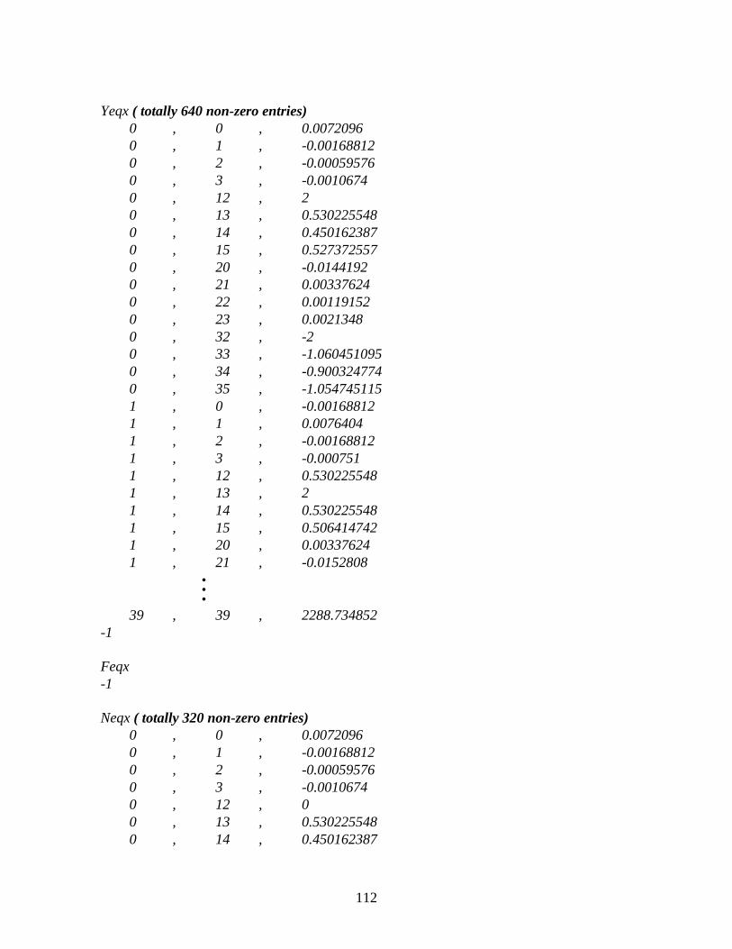
Yeqx ( totally 640 non-zero entries) 0 , 0 , 0.0072096 0 , 1 , -0.00168812 0 , 2 , -0.00059576 0 , 3 , -0.0010674 0 , 12 , 2 0 , 13 , 0.530225548 0 , 14 , 0.450162387 0 , 15 , 0.527372557 0 , 20 , -0.0144192 0 , 21 , 0.00337624 0 , 22 , 0.00119152 0 , 23 , 0.0021348 0 , 32 , -2 0 , 33 , -1.060451095 0 , 34 , -0.900324774 0 , 35 , -1.054745115 1 , 0 , -0.00168812 1 , 1 , 0.0076404 1 , 2 , -0.00168812 1 , 3 , -0.000751 1 , 12 , 0.530225548 1 , 13 , 2 1 , 14 , 0.530225548 1 , 15 , 0.506414742 1 , 20 , 0.00337624 1 , 21 , -0.0152808

39 , 39 , 2288.734852 -1

Feqx -1

Neqx ( totally 320 non-zero entries) 0 , 0 , 0.0072096 0 , 1 , -0.00168812 0 , 2 , -0.00059576 0 , 3 , -0.0010674 0 , 12 , 0 0 , 13 , 0.530225548 0 , 14 , 0.450162387

112

0 , 15 , 0.527372557 1 , 0 , -0.00168812 1 , 1 , 0.0076404 1 , 2 , -0.00168812 1 , 3 , -0.000751 1 , 12 , 0.530225548 1 , 13 , 0 1 , 14 , 0.530225548 1 , 15 , 0.506414742 2 , 0 , -0.00059576 2 , 1 , -0.00168812 2 , 2 , 0.0072096 2 , 3 , -0.000399056 2 , 12 , 0.450162387 2 , 13 , 0.530225548 2 , 14 , 0 2 , 15 , 0.451167214 3 , 0 , -0.0010674 3 , 1 , -0.000751 3 , 2 , -0.000399056 3 , 3 , 0.0044192 3 , 12 , 0.264879236 3 , 13 , 0.25435292 3 , 14 , 0.226604182 3 , 15 , 0 4 , 4 , 0.0072096

39 , 19 , -2781.311065 -1 Meq 0 , 0 , 1 1 , 1 , 1 2 , 2 , 1 3 , 3 , 1 4 , 4 , 1 5 , 5 , 1 6 , 6 , 1 7 , 7 , 1 20 , 0 , -0.5 21 , 1 , -0.5 22 , 2 , -0.5 23 , 3 , -0.5 24 , 4 , -0.5

113

25 , 5 , -0.5 26 , 6 , -0.5 27 , 7 , -0.5 -1

Keq -1

E3. Three Phase Multi-section Transmission Line SCAQCF Measurement Model

For multi-section transmission line, the actual measurements are: Six currents at both side of the transmission line, at time t (phase A, phase B, and phase C); Six voltages at both side of the transmission line, at time t (phase A-N, phase B-N, phase C-N); Six currents at both side of the transmission line, at time tm=t-h/2 (phase A, phase B, and phase C); Six voltages at both side of the transmission line, at time tm=t-h/2 (phase A-N, phase B-N, phase C-N); The pseudo measurements are: Two neutral currents at both side of the transmission line, at time t (phase N); Two neutral voltages at both side of the transmission line, at time t (phase N); Two neutral currents at both side of the transmission line, at time tm=t-h/2 (phase N); Two neutral voltages at both side of the transmission line, at time tm=t-h/2 (phase N); The virtual measurements are: Twelve measurements with zero value at the left side of the equations at time t, including four virtual current measurements and eight virtual voltage measurements; Twelve measurements with zero value at the left side of the equations at time tm=t-h/2, including four virtual current measurements and eight virtual voltage measurements; The measurement channel list: MeasurementType, 17 MeasStdDev, 40.41 MeasTerminal, 0 MeasurementEnd MeasurementType, 17 MeasStdDev, 40.41 MeasTerminal, 1 MeasurementEnd MeasurementType, 17 MeasStdDev, 40.41 MeasTerminal, 2 MeasurementEnd MeasurementType, 17

114

MeasStdDev, 40.41 MeasTerminal, 4 MeasurementEnd MeasurementType, 17 MeasStdDev, 40.41 MeasTerminal, 5 MeasurementEnd MeasurementType, 17 MeasStdDev, 40.41 MeasTerminal, 6 MeasurementEnd MeasurementType, 16 MeasStdDev, 5000 MeasTerminal, 0, 3 MeasurementEnd MeasurementType, 16 MeasStdDev, 5000 MeasTerminal, 1, 3 MeasurementEnd MeasurementType, 16 MeasStdDev, 5000 MeasTerminal, 2, 3 MeasurementEnd MeasurementType, 16 MeasStdDev, 5000 MeasTerminal, 4, 7 MeasurementEnd MeasurementType, 16 MeasStdDev, 5000 MeasTerminal, 5, 7 MeasurementEnd MeasurementType, 16 MeasStdDev, 5000 MeasTerminal, 6, 7 MeasurementEnd MeasurementType, 27 MeasStdDev, 404.1 MeasTerminal, 3 MeasurementEnd MeasurementType, 27 MeasStdDev, 404.1 MeasTerminal, 7 MeasurementEnd MeasurementType, 25 MeasStdDev, 50000 MeasTerminal, 3

115

MeasurementEnd MeasurementType, 25 MeasStdDev, 50000 MeasTerminal, 7 MeasurementEnd MeasurementType, 24 MeasStdDev, 4.041 MeasTerminal, 8 MeasurementEnd MeasurementType, 24 MeasStdDev, 4.041 MeasTerminal, 9 MeasurementEnd MeasurementType, 24 MeasStdDev, 4.041 MeasTerminal, 10 MeasurementEnd MeasurementType, 24 MeasStdDev, 4.041 MeasTerminal, 11 MeasurementEnd MeasurementType, 24 MeasStdDev, 500 MeasTerminal, 12 MeasurementEnd MeasurementType, 24 MeasStdDev, 500 MeasTerminal, 13 MeasurementEnd MeasurementType, 24 MeasStdDev, 500 MeasTerminal, 14 MeasurementEnd MeasurementType, 24 MeasStdDev, 500 MeasTerminal, 15 MeasurementEnd MeasurementType, 24 MeasStdDev, 500 MeasTerminal, 16 MeasurementEnd MeasurementType, 24 MeasStdDev, 500 MeasTerminal, 17 MeasurementEnd MeasurementType, 24

116

MeasStdDev, 500 MeasTerminal, 18 MeasurementEnd MeasurementType, 24 MeasStdDev, 500 MeasTerminal, 19 MeasurementEnd Based on the device model and the measurement channel list, the standard SCAQCF equations for the measurement model are given below:


= + + + + + − + − + − +


where:

11 12 13 14

21 22 23 24,

31 32 33 34

41 42 43 44

0 0 0 0 0 0 00 0 0 0 0 0 0

0 0 0 0 0 0 00 0 0 0 0 0 0

m x

TT

Y Y Y YY Y Y Y

YT

TY Y Y YY Y Y Y

=

11 12

21 22,

31 32

41 42

0 0 0 00 0 0 0 0 0 0 00 0 0 0

m x

N NN N

N

N NN N

= −

8 8

,

8 8

0 0 0 00 0 0 0

0 0 0

0 0 0 00 0 0 00.5 0

0 0

m x

I

M

I

×

×

= −

1 0 0 10 1 0 10 0 1 10 0 0 1

T

− − = −

And, the definitions of ijY and ijN are given in Appendix E.2.

117

Appendix F: Time Domain SCAQCF Model – Single Phase Saturable Core Variable Tap Transformer Protection

This document describes the model of a single-phase, two-winding, saturable-core variable tap transformer. The model is based on a standard transformer equivalent circuit, but the core magnetizing reactance is modeled as a nonlinear inductor with a current characteristic equation of high degree of nonlinearity.

F1. Single Phase Saturable Core Transformer Compact Model

The overall physical model of a single phase, saturable core variable tap transformer is illustrated in Figure F1. Core losses are also considered in the model, expressed by the conductance𝑔𝑔𝑐𝑐. The “numerical stabilizers” 𝑔𝑔𝑚𝑚1,𝑔𝑔𝑚𝑚2,𝑔𝑔𝑚𝑚3 𝑎𝑎𝑒𝑒𝑎𝑎 𝑔𝑔𝑚𝑚4 are introduced to eliminate possible numerical problems. The compact model is based on the circuit analysis of the equivalent circuit of Figure F1.

4 ( )v t

6 ( )i t5 ( )i t

4 ( )i t

3 ( )i t

2 ( )i t

1( )i t

( )mi t

1( )ci t

2 ( )ci t

1 ( )Li t 3 ( )Li t

4 ( )Li t

1rα1( )v t

2 ( )v t

3 ( )v t

5 ( )v t

6 ( )v t

2 ( )Li t

1(1 )rα−

1Lα

1(1 )Lα−

2(1 )Lβ−

2Lβ

2rβ

2(1 )rβ−

cg ML

1sg

2sg

3sg

4sg

+ +

+−

−

1( )ce t 3 ( )ce t

2 ( )ce t4 ( )ce t

Figure F.1: Single Phase Transformer Equivalent Circuit

The model with nonlinear magnetizing inductor in the compact form is described by equations (3.1) through (3.18)

𝑖𝑖1(𝑜𝑜) = 𝑖𝑖𝐿𝐿1(𝑜𝑜) + 𝑔𝑔𝑚𝑚1𝛼𝛼𝐿𝐿1𝑎𝑎𝑖𝑖𝐿𝐿1(𝑜𝑜)𝑎𝑎𝑜𝑜

(3.1)

𝑖𝑖2(𝑜𝑜) = 𝑖𝑖𝐿𝐿2(𝑜𝑜) + 𝑔𝑔𝑚𝑚2(1 − 𝛼𝛼)𝐿𝐿1𝑎𝑎𝑖𝑖𝐿𝐿2(𝑜𝑜)𝑎𝑎𝑜𝑜

(3.2)

𝑖𝑖3(𝑜𝑜) = 𝑖𝑖𝐿𝐿3(𝑜𝑜) + 𝑔𝑔𝑚𝑚3𝛽𝛽𝐿𝐿2𝑎𝑎𝑖𝑖𝐿𝐿3(𝑜𝑜)𝑎𝑎𝑜𝑜

(3.3)

118

𝑖𝑖4(𝑜𝑜) = 𝑖𝑖𝐿𝐿4(𝑜𝑜) + 𝑔𝑔𝑚𝑚4(1 − 𝛽𝛽)𝐿𝐿2𝑎𝑎𝑖𝑖𝐿𝐿4(𝑜𝑜)𝑎𝑎𝑜𝑜

(3.4)

𝑖𝑖5(𝑜𝑜) = −𝑖𝑖1(𝑜𝑜) − 𝑖𝑖2(𝑜𝑜) (3.5)

𝑖𝑖6(𝑜𝑜) = −𝑖𝑖3(𝑜𝑜) − 𝑖𝑖4(𝑜𝑜) (3.6)

0 = 𝑣𝑣1(𝑜𝑜) − 𝑣𝑣5(𝑜𝑜) − 𝛼𝛼𝑒𝑒1𝑖𝑖1(𝑜𝑜) − 𝛼𝛼𝐿𝐿1𝑎𝑎𝑖𝑖𝐿𝐿1(𝑜𝑜)𝑎𝑎𝑜𝑜

− 𝑒𝑒𝑐𝑐1(𝑜𝑜) (3.7)

0 = 𝑣𝑣2(𝑜𝑜) − 𝑣𝑣5(𝑜𝑜) − (1 − 𝛼𝛼)𝑒𝑒1𝑖𝑖2(𝑜𝑜) − (1 − 𝛼𝛼)𝐿𝐿1𝑎𝑎𝑖𝑖𝐿𝐿2(𝑜𝑜)𝑎𝑎𝑜𝑜

+ 𝑒𝑒𝑐𝑐2(𝑜𝑜) (3.8)

0 = 𝑣𝑣3(𝑜𝑜) − 𝑣𝑣6(𝑜𝑜) − 𝛽𝛽𝑒𝑒2𝑖𝑖3(𝑜𝑜) − 𝛽𝛽𝐿𝐿2𝑎𝑎𝑖𝑖𝐿𝐿3(𝑜𝑜)𝑎𝑎𝑜𝑜

− 𝑒𝑒𝑐𝑐3(𝑜𝑜) (3.9)

0 = 𝑣𝑣4(𝑜𝑜) − 𝑣𝑣6(𝑜𝑜) − (1 − 𝛽𝛽)𝑒𝑒2𝑖𝑖4(𝑜𝑜) − (1 − 𝛽𝛽)𝐿𝐿2𝑎𝑎𝑖𝑖𝐿𝐿4(𝑜𝑜)𝑎𝑎𝑜𝑜

+ 𝑒𝑒𝑐𝑐4(𝑜𝑜) (3.10)

0 = 𝛼𝛼𝑁𝑁1𝑖𝑖𝑐𝑐1(𝑜𝑜) − (1 − 𝛼𝛼)𝑁𝑁1𝑖𝑖𝑐𝑐2(𝑜𝑜) + 𝛽𝛽𝑁𝑁2𝑖𝑖3(𝑜𝑜) − (1 − 𝛽𝛽)𝑁𝑁2𝑖𝑖4(𝑜𝑜) (3.11)

0 = 𝑒𝑒𝑐𝑐1(𝑜𝑜) − 𝛼𝛼𝑎𝑎λ (𝑜𝑜)𝑎𝑎𝑜𝑜

(3.12)

0 = 𝑒𝑒𝑐𝑐2(𝑜𝑜) − (1 − 𝛼𝛼)𝑎𝑎λ (𝑜𝑜)𝑎𝑎𝑜𝑜

(3.13)

0 = 𝑒𝑒𝑐𝑐3(𝑜𝑜) − 𝛽𝛽𝑁𝑁2𝑁𝑁1

𝑎𝑎λ (𝑜𝑜)𝑎𝑎𝑜𝑜

(3.14)

0 = 𝑒𝑒𝑐𝑐4(𝑜𝑜) − (1 − 𝛽𝛽)𝑁𝑁2𝑁𝑁1

𝑎𝑎λ (𝑜𝑜)𝑎𝑎𝑜𝑜

(3.15)

0 = −𝑖𝑖1(𝑜𝑜) + 𝑖𝑖𝑐𝑐1(𝑜𝑜) + 𝑖𝑖𝑚𝑚(𝑜𝑜) + 𝑔𝑔𝑐𝑐�𝑒𝑒𝑐𝑐1(𝑜𝑜) + 𝑒𝑒𝑐𝑐2(𝑜𝑜)� (3.16)

0 = −𝑖𝑖2(𝑜𝑜) + 𝑖𝑖𝑐𝑐2(𝑜𝑜) − 𝑖𝑖𝑚𝑚(𝑜𝑜) − 𝑔𝑔𝑐𝑐�𝑒𝑒𝑐𝑐1(𝑜𝑜) + 𝑒𝑒𝑐𝑐2(𝑜𝑜)� (3.17)

0 = 𝑖𝑖𝑚𝑚(𝑜𝑜) − 𝑖𝑖0 �λ (𝑜𝑜)

λ 0�𝑛𝑛

𝑒𝑒𝑖𝑖𝑔𝑔𝑒𝑒( λ (𝑜𝑜)) (3.18)

0.9 < 𝑜𝑜(𝑜𝑜) < 1.1

There are 18 states variables

𝑋𝑋 = �𝑣𝑣1(𝑜𝑜), 𝑣𝑣2(𝑜𝑜), 𝑣𝑣3(𝑜𝑜), 𝑣𝑣4(𝑜𝑜), 𝑣𝑣5(𝑜𝑜), 𝑣𝑣6(𝑜𝑜),𝑖𝑖𝐿𝐿1(𝑜𝑜), 𝑖𝑖𝐿𝐿2(𝑜𝑜), 𝑖𝑖𝐿𝐿3(𝑜𝑜), 𝑖𝑖𝐿𝐿4(𝑜𝑜), λ (𝑜𝑜)

𝑒𝑒𝑐𝑐1(𝑜𝑜), 𝑒𝑒𝑐𝑐2(𝑜𝑜), 𝑒𝑒𝑐𝑐3(𝑜𝑜), 𝑒𝑒𝑐𝑐4(𝑜𝑜), 𝑖𝑖𝑐𝑐2(𝑜𝑜), 𝑖𝑖𝑐𝑐2(𝑜𝑜), 𝑖𝑖𝑚𝑚(𝑜𝑜)�

And 6 though variables 𝐼𝐼 = [𝑖𝑖1(𝑜𝑜), 𝑖𝑖2(𝑜𝑜), 𝑖𝑖3(𝑜𝑜), 𝑖𝑖4(𝑜𝑜), 𝑖𝑖5(𝑜𝑜), 𝑖𝑖6(𝑜𝑜)]

And 1 control variable 𝑈𝑈 = [𝑜𝑜(𝑜𝑜)]

119

F2. Single Phase Saturable Core Transformer Quadratic Model

The model is quadratized by introducing additional internal state variables, so that the nth exponent is replaced by equations of at most quadratic degree. Since the exact degree of nonlinearity is not known until the user specifies it, the model performs automatic quadratization of the equations. A special procedure is used, so that the model is quadratized using the minimum number of additional internal states, while also maintaining the scarcity of the resulting equations. The methodology is based on expressing the exponent in binary form. The binary representation provides all the information about the number of new variables and equations that need to be introduced and about the form of the equations (products of new variables). The procedure is described later. Following this procedure the model can be converted into the standard quadratized form: 𝑖𝑖1(𝑜𝑜) = 𝑖𝑖𝐿𝐿1(𝑜𝑜) + 𝑔𝑔𝑚𝑚1𝛼𝛼𝐿𝐿1𝑧𝑧1(𝑜𝑜) (4.1)

𝑖𝑖2(𝑜𝑜) = 𝑖𝑖𝐿𝐿2(𝑜𝑜) + 𝑔𝑔𝑚𝑚2(1 − 𝛼𝛼)𝐿𝐿1𝑧𝑧2(𝑜𝑜) (4.2)

𝑖𝑖3(𝑜𝑜) = 𝑖𝑖𝐿𝐿3(𝑜𝑜) + 𝑔𝑔𝑚𝑚3𝛽𝛽𝐿𝐿2𝑧𝑧3(𝑜𝑜) (4.3)

𝑖𝑖4(𝑜𝑜) = 𝑖𝑖𝐿𝐿4(𝑜𝑜) + 𝑔𝑔𝑚𝑚4(1 − 𝛽𝛽)𝐿𝐿2𝑧𝑧4(𝑜𝑜) (4.4)

𝑖𝑖5(𝑜𝑜) = −𝑖𝑖𝐿𝐿1(𝑜𝑜) − 𝑖𝑖𝐿𝐿2(𝑜𝑜) − 𝑔𝑔𝑚𝑚1𝛼𝛼𝐿𝐿1𝑧𝑧1(𝑜𝑜) − 𝑔𝑔𝑚𝑚2(1 − 𝛼𝛼)𝐿𝐿1𝑧𝑧2(𝑜𝑜) (4.5)

𝑖𝑖6(𝑜𝑜) = −𝑖𝑖𝐿𝐿3(𝑜𝑜) − 𝑖𝑖𝐿𝐿4(𝑜𝑜) − 𝑔𝑔𝑚𝑚3𝛽𝛽𝐿𝐿2𝑧𝑧3(𝑜𝑜) − 𝑔𝑔𝑚𝑚4(1 − 𝛽𝛽)𝐿𝐿2𝑧𝑧4(𝑜𝑜) (4.6)

0 = 𝑧𝑧1(𝑜𝑜) −𝑎𝑎𝑖𝑖𝐿𝐿1(𝑜𝑜)𝑎𝑎𝑜𝑜

(4.7)


(4.8)


(4.9)


(4.10)

0 = 𝑧𝑧5(𝑜𝑜) −𝑎𝑎λ (𝑜𝑜)𝑎𝑎𝑜𝑜

(4.11)

0 = 𝑣𝑣1(𝑜𝑜) − 𝑣𝑣5(𝑜𝑜) − 𝛼𝛼𝑒𝑒1(𝑖𝑖𝐿𝐿1(𝑜𝑜) + 𝑔𝑔𝑚𝑚1𝛼𝛼𝐿𝐿1𝑧𝑧1(𝑜𝑜)) − 𝛼𝛼𝐿𝐿1𝑧𝑧1(𝑜𝑜) − 𝑒𝑒𝑐𝑐1(𝑜𝑜) (4.12)

0 = 𝑣𝑣2(𝑜𝑜) − 𝑣𝑣5(𝑜𝑜) − (1 − 𝛼𝛼)𝑒𝑒1(𝑖𝑖𝐿𝐿2(𝑜𝑜) + 𝑔𝑔𝑚𝑚2(1 − 𝛼𝛼)𝐿𝐿1𝑧𝑧2(𝑜𝑜))− (1 − 𝛼𝛼)𝐿𝐿1𝑧𝑧2(𝑜𝑜) + 𝑒𝑒𝑐𝑐2(𝑜𝑜)

(4.13)

0 = 𝑣𝑣3(𝑜𝑜) − 𝑣𝑣6(𝑜𝑜) − 𝛽𝛽𝑒𝑒2(𝑖𝑖𝐿𝐿3(𝑜𝑜) + 𝑔𝑔𝑚𝑚3𝛽𝛽𝐿𝐿2𝑧𝑧3(𝑜𝑜)) − 𝛽𝛽𝐿𝐿2𝑧𝑧3(𝑜𝑜) − 𝑒𝑒𝑐𝑐3(𝑜𝑜) (4.14)

0 = 𝑣𝑣4(𝑜𝑜) − 𝑣𝑣6(𝑜𝑜) − (1 − 𝛽𝛽)𝑒𝑒2(𝑖𝑖𝐿𝐿4(𝑜𝑜) + 𝑔𝑔𝑚𝑚4(1 − 𝛽𝛽)𝐿𝐿2𝑧𝑧4(𝑜𝑜))− (1 − 𝛽𝛽)𝐿𝐿2𝑧𝑧4(𝑜𝑜) + 𝑒𝑒𝑐𝑐4(𝑜𝑜)

(4.15)

120

0 = 𝛼𝛼𝑁𝑁1𝑖𝑖𝑐𝑐1(𝑜𝑜) − (1 − 𝛼𝛼)𝑁𝑁1𝑖𝑖𝑐𝑐2(𝑜𝑜) + 𝛽𝛽𝑁𝑁2�𝑖𝑖𝐿𝐿3(𝑜𝑜) + 𝑔𝑔𝑚𝑚3𝛽𝛽𝐿𝐿2𝑧𝑧3(𝑜𝑜)� −

(1 − 𝛽𝛽)𝑁𝑁2(𝑖𝑖𝐿𝐿4(𝑜𝑜) + 𝑔𝑔𝑚𝑚4(1 − 𝛽𝛽)𝐿𝐿2𝑧𝑧4(𝑜𝑜)) (4.16)

0 = 𝑒𝑒𝑐𝑐1(𝑜𝑜) − 𝛼𝛼𝑧𝑧5(𝑜𝑜) (4.17)

0 = 𝑒𝑒𝑐𝑐2(𝑜𝑜) − (1 − 𝛼𝛼)𝑧𝑧5(𝑜𝑜) (4.18)


𝑧𝑧5(𝑜𝑜) (4.19)


𝑧𝑧5(𝑜𝑜) (4.20)

0 = −𝑖𝑖𝐿𝐿1(𝑜𝑜) − 𝑔𝑔𝑚𝑚1𝛼𝛼𝐿𝐿1𝑧𝑧1(𝑜𝑜) + 𝑖𝑖𝑐𝑐1(𝑜𝑜) + 𝑖𝑖𝑚𝑚(𝑜𝑜) + 𝑔𝑔𝑐𝑐�𝑒𝑒𝑐𝑐1(𝑜𝑜) + 𝑒𝑒𝑐𝑐2(𝑜𝑜)� (4.21)

0 = −𝑖𝑖𝐿𝐿2(𝑜𝑜) − 𝑔𝑔𝑚𝑚2(1 − 𝛼𝛼)𝐿𝐿1𝑧𝑧2(𝑜𝑜) + 𝑖𝑖𝑐𝑐2(𝑜𝑜) − 𝑖𝑖𝑚𝑚(𝑜𝑜)− 𝑔𝑔𝑐𝑐�𝑒𝑒𝑐𝑐1(𝑜𝑜) + 𝑒𝑒𝑐𝑐2(𝑜𝑜)�

(4.22)

0 = 𝑖𝑖𝑚𝑚(𝑜𝑜) − 𝑖𝑖0 ∙ 𝑦𝑦𝑚𝑚(𝑜𝑜) ∙ �𝑒𝑒𝑖𝑖𝑔𝑔𝑒𝑒( λ (𝑜𝑜))�𝑛𝑛+1

(4.23)

0 = 𝑦𝑦1(𝑜𝑜) −λ (𝑜𝑜)2

λ 02 (4.24)

0 = 𝑦𝑦2(𝑜𝑜) − 𝑦𝑦1(𝑜𝑜)2 (4.25)

⋯⋯

⋯⋯

0 = 𝑦𝑦𝑚𝑚1(𝑜𝑜) − 𝑦𝑦𝑚𝑚1−1(𝑜𝑜)2 (4.23+m1)

0 = 𝑦𝑦𝑚𝑚1+1(𝑜𝑜) − 𝑦𝑦𝑑𝑑1(𝑜𝑜) ∙ 𝑦𝑦𝑗𝑗1(𝑜𝑜) (4.23+m1+1)

0 = 𝑦𝑦𝑚𝑚1+2(𝑜𝑜) − 𝑦𝑦𝑚𝑚1+1(𝑜𝑜) ∙ 𝑦𝑦𝑗𝑗2(𝑜𝑜) (4.23+m1+2)

⋯⋯

⋯⋯

�

0 = 𝑦𝑦𝑚𝑚(𝑜𝑜) − 𝑦𝑦𝑚𝑚−1(𝑜𝑜) ∙ 𝑦𝑦𝑗𝑗𝑚𝑚2(𝑜𝑜) , 𝑖𝑖𝑓𝑓 𝑒𝑒 𝑒𝑒𝑣𝑣𝑒𝑒𝑒𝑒

0 = 𝑦𝑦𝑚𝑚(𝑜𝑜) − 𝑦𝑦𝑚𝑚−1(𝑜𝑜) ∙λ (𝑜𝑜)

λ0

, 𝑖𝑖𝑓𝑓 𝑒𝑒 𝑜𝑜𝑎𝑎𝑎𝑎 (4.23+m)

0.9 < 𝑜𝑜(𝑜𝑜) < 1.1

There are 23+m states

121

𝑋𝑋(𝑜𝑜) =

⎣⎢⎢⎢⎢⎡𝑣𝑣1(𝑜𝑜), 𝑣𝑣2(𝑜𝑜), 𝑣𝑣3(𝑜𝑜), 𝑣𝑣4(𝑜𝑜), 𝑣𝑣5(𝑜𝑜), 𝑣𝑣6(𝑜𝑜),𝑖𝑖𝐿𝐿1(𝑜𝑜), 𝑖𝑖𝐿𝐿2(𝑜𝑜), 𝑖𝑖𝐿𝐿3(𝑜𝑜), 𝑖𝑖𝐿𝐿4(𝑜𝑜), λ (𝑜𝑜),𝑧𝑧1(𝑜𝑜), 𝑧𝑧2(𝑜𝑜), 𝑧𝑧3(𝑜𝑜), 𝑧𝑧4(𝑜𝑜), 𝑧𝑧5(𝑜𝑜),

𝑒𝑒𝑐𝑐1(𝑜𝑜), 𝑒𝑒𝑐𝑐2(𝑜𝑜), 𝑒𝑒𝑐𝑐3(𝑜𝑜), 𝑒𝑒𝑐𝑐4(𝑜𝑜), 𝑖𝑖𝑐𝑐1(𝑜𝑜), 𝑖𝑖𝑐𝑐2(𝑜𝑜),𝑖𝑖𝑚𝑚(𝑜𝑜),𝑦𝑦1(𝑜𝑜),𝑦𝑦2(𝑜𝑜),⋯⋯ ,𝑦𝑦𝑚𝑚(𝑜𝑜) ⎦

⎥⎥⎥⎥⎤

And 6 though variables 𝐼𝐼 = [𝑖𝑖1(𝑜𝑜), 𝑖𝑖2(𝑜𝑜), 𝑖𝑖3(𝑜𝑜), 𝑖𝑖4(𝑜𝑜), 𝑖𝑖5(𝑜𝑜), 𝑖𝑖6(𝑜𝑜)]

And 1 control variable 𝑈𝑈 = [𝑜𝑜(𝑜𝑜)]

Based on the above formulation, the number of additional internal states and equations m is computed as follows:

21 mmm += where:

))(int(log21 nm = =2m (# of ones in the binary representation of n ) – 1

The sets of indices i and j in the last set of equations are provided by positions of ones in the binary representation of n . The values of these indices are equal to the values of the power of 2 corresponding to that position, meaning that the right most positions is indexed 0 and the left most indexed ))(int(log2 n . The variable 0y is by definition equal to λ , so it is not used and appears as

λ in the equations. If the symbol 0y was used instead of λ then only the first case in equation (M4.23+m1+m2) would have been necessary, since this would include the second when the index becomes 0. However, since λ is physically related to flux, for the time being the use of this symbol is preferred instead.

F3. Single Phase Saturable Core Transformer SCAQCF Device Model

The differential equations in above model are integrated with the quadratic integration method and the equations that are algebraic are sufficed to be written at times t and tm. The SCAQCF model yields the following model. At Time t 𝑖𝑖1(𝑜𝑜) = 𝑖𝑖𝐿𝐿1(𝑜𝑜) + 𝑔𝑔𝑚𝑚1𝛼𝛼𝐿𝐿1𝑧𝑧1(𝑜𝑜)

𝑖𝑖2(𝑜𝑜) = 𝑖𝑖𝐿𝐿2(𝑜𝑜) + 𝑔𝑔𝑚𝑚2(1 − 𝛼𝛼)𝐿𝐿1𝑧𝑧2(𝑜𝑜)

𝑖𝑖3(𝑜𝑜) = 𝑖𝑖𝐿𝐿3(𝑜𝑜) + 𝑔𝑔𝑚𝑚3𝛽𝛽𝐿𝐿2𝑧𝑧3(𝑜𝑜)

𝑖𝑖4(𝑜𝑜) = 𝑖𝑖𝐿𝐿4(𝑜𝑜) + 𝑔𝑔𝑚𝑚4(1 − 𝛽𝛽)𝐿𝐿2𝑧𝑧4(𝑜𝑜)

𝑖𝑖5(𝑜𝑜) = −𝑖𝑖𝐿𝐿1(𝑜𝑜) − 𝑖𝑖𝐿𝐿2(𝑜𝑜) − 𝑔𝑔𝑚𝑚1𝛼𝛼𝐿𝐿1𝑧𝑧1(𝑜𝑜) − 𝑔𝑔𝑚𝑚2(1 − 𝛼𝛼)𝐿𝐿1𝑧𝑧2(𝑜𝑜)

122

𝑖𝑖6(𝑜𝑜) = −𝑖𝑖𝐿𝐿3(𝑜𝑜) − 𝑖𝑖𝐿𝐿4(𝑜𝑜) − 𝑔𝑔𝑚𝑚3𝛽𝛽𝐿𝐿2𝑧𝑧3(𝑜𝑜) − 𝑔𝑔𝑚𝑚4(1 − 𝛽𝛽)𝐿𝐿2𝑧𝑧4(𝑜𝑜)

0 = 𝑖𝑖𝐿𝐿1(𝑜𝑜) −ℎ6𝑧𝑧1(𝑜𝑜) −

2ℎ3𝑧𝑧1(𝑜𝑜𝑚𝑚) − 𝑖𝑖𝐿𝐿1(𝑜𝑜 − ℎ) −

ℎ6𝑧𝑧1(𝑜𝑜 − ℎ)










0 = λ (𝑜𝑜) −ℎ6𝑧𝑧5(𝑜𝑜) −

2ℎ3𝑧𝑧5(𝑜𝑜𝑚𝑚) − λ (𝑜𝑜 − ℎ) −


0 = 𝑣𝑣1(𝑜𝑜) − 𝑣𝑣5(𝑜𝑜) − 𝛼𝛼𝑒𝑒1(𝑖𝑖𝐿𝐿1(𝑜𝑜) + 𝑔𝑔𝑚𝑚1𝛼𝛼𝐿𝐿1𝑧𝑧1(𝑜𝑜)) − 𝛼𝛼𝐿𝐿1𝑧𝑧1(𝑜𝑜) − 𝑒𝑒𝑐𝑐1(𝑜𝑜)


0 = 𝑣𝑣3(𝑜𝑜) − 𝑣𝑣6(𝑜𝑜) − 𝛽𝛽𝑒𝑒2(𝑖𝑖𝐿𝐿3(𝑜𝑜) + 𝑔𝑔𝑚𝑚3𝛽𝛽𝐿𝐿2𝑧𝑧3(𝑜𝑜)) − 𝛽𝛽𝐿𝐿2𝑧𝑧3(𝑜𝑜) − 𝑒𝑒𝑐𝑐3(𝑜𝑜)



(1 − 𝛽𝛽)𝑁𝑁2(𝑖𝑖𝐿𝐿4(𝑜𝑜) + 𝑔𝑔𝑚𝑚4(1 − 𝛽𝛽)𝐿𝐿2𝑧𝑧4(𝑜𝑜))

0 = 𝑒𝑒𝑐𝑐1(𝑜𝑜) − 𝛼𝛼𝑧𝑧5(𝑜𝑜)

0 = 𝑒𝑒𝑐𝑐2(𝑜𝑜) − (1 − 𝛼𝛼)𝑧𝑧5(𝑜𝑜)


𝑧𝑧5(𝑜𝑜)


𝑧𝑧5(𝑜𝑜)

0 = −𝑖𝑖𝐿𝐿1(𝑜𝑜) − 𝑔𝑔𝑚𝑚1𝛼𝛼𝐿𝐿1𝑧𝑧1(𝑜𝑜) + 𝑖𝑖𝑐𝑐1(𝑜𝑜) + 𝑖𝑖𝑚𝑚(𝑜𝑜) + 𝑔𝑔𝑐𝑐�𝑒𝑒𝑐𝑐1(𝑜𝑜) + 𝑒𝑒𝑐𝑐2(𝑜𝑜)�



0 = 𝑦𝑦1(𝑜𝑜) −λ (𝑜𝑜)2

λ 02

123

0 = 𝑦𝑦2(𝑜𝑜) − 𝑦𝑦1(𝑜𝑜)2

⋯⋯

⋯⋯

0 = 𝑦𝑦𝑚𝑚1(𝑜𝑜) − 𝑦𝑦𝑚𝑚1−1(𝑜𝑜)2

0 = 𝑦𝑦𝑚𝑚1+1(𝑜𝑜) − 𝑦𝑦𝑑𝑑1(𝑜𝑜) ∙ 𝑦𝑦𝑗𝑗1(𝑜𝑜)

0 = 𝑦𝑦𝑚𝑚1+2(𝑜𝑜) − 𝑦𝑦𝑚𝑚1+1(𝑜𝑜) ∙ 𝑦𝑦𝑗𝑗2(𝑜𝑜)

⋯⋯

⋯⋯

�



λ0

, 𝑖𝑖𝑓𝑓 𝑒𝑒 𝑜𝑜𝑎𝑎𝑎𝑎

0.9 < 𝑜𝑜(𝑜𝑜) < 1.1

At Time tm 𝑖𝑖1(𝑜𝑜𝑚𝑚) = 𝑖𝑖𝐿𝐿1(𝑜𝑜𝑚𝑚) + 𝑔𝑔𝑚𝑚1𝛼𝛼𝐿𝐿1𝑧𝑧1(𝑜𝑜𝑚𝑚)

𝑖𝑖2(𝑜𝑜𝑚𝑚) = 𝑖𝑖𝐿𝐿2(𝑜𝑜𝑚𝑚) + 𝑔𝑔𝑚𝑚2(1 − 𝛼𝛼)𝐿𝐿1𝑧𝑧2(𝑜𝑜𝑚𝑚)

𝑖𝑖3(𝑜𝑜𝑚𝑚) = 𝑖𝑖𝐿𝐿3(𝑜𝑜𝑚𝑚) + 𝑔𝑔𝑚𝑚3𝛽𝛽𝐿𝐿2𝑧𝑧3(𝑜𝑜𝑚𝑚)

𝑖𝑖4(𝑜𝑜𝑚𝑚) = 𝑖𝑖𝐿𝐿4(𝑜𝑜𝑚𝑚) + 𝑔𝑔𝑚𝑚4(1 − 𝛽𝛽)𝐿𝐿2𝑧𝑧4(𝑜𝑜𝑚𝑚)

𝑖𝑖5(𝑜𝑜𝑚𝑚) = −𝑖𝑖𝐿𝐿1(𝑜𝑜𝑚𝑚) − 𝑖𝑖𝐿𝐿2(𝑜𝑜𝑚𝑚) − 𝑔𝑔𝑚𝑚1𝛼𝛼𝐿𝐿1𝑧𝑧1(𝑜𝑜𝑚𝑚) − 𝑔𝑔𝑚𝑚2(1 − 𝛼𝛼)𝐿𝐿1𝑧𝑧2(𝑜𝑜𝑚𝑚)

𝑖𝑖6(𝑜𝑜𝑚𝑚) = −𝑖𝑖𝐿𝐿3(𝑜𝑜𝑚𝑚) − 𝑖𝑖𝐿𝐿4(𝑜𝑜𝑚𝑚) − 𝑔𝑔𝑚𝑚3𝛽𝛽𝐿𝐿2𝑧𝑧3(𝑜𝑜𝑚𝑚) − 𝑔𝑔𝑚𝑚4(1 − 𝛽𝛽)𝐿𝐿2𝑧𝑧4(𝑜𝑜𝑚𝑚)

0 = 𝑖𝑖𝐿𝐿1(𝑜𝑜𝑚𝑚) +ℎ

24𝑧𝑧1(𝑜𝑜) −

ℎ3𝑧𝑧1(𝑜𝑜𝑚𝑚) − 𝑖𝑖𝐿𝐿1(𝑜𝑜 − ℎ) −

5ℎ24

𝑧𝑧1(𝑜𝑜 − ℎ)


24𝑧𝑧2(𝑜𝑜) −


5ℎ24



24𝑧𝑧3(𝑜𝑜) −


5ℎ24



24𝑧𝑧4(𝑜𝑜) −


5ℎ24


0 = λ (𝑜𝑜𝑚𝑚) +ℎ

24𝑧𝑧5(𝑜𝑜) −

ℎ3𝑧𝑧5(𝑜𝑜𝑚𝑚) − λ (𝑜𝑜 − ℎ) −

5ℎ24


124

0 = 𝑣𝑣1(𝑜𝑜𝑚𝑚) − 𝑣𝑣5(𝑜𝑜𝑚𝑚) − 𝛼𝛼𝑒𝑒1(𝑖𝑖𝐿𝐿1(𝑜𝑜𝑚𝑚) + 𝑔𝑔𝑚𝑚1𝛼𝛼𝐿𝐿1𝑧𝑧1(𝑜𝑜𝑚𝑚)) − 𝛼𝛼𝐿𝐿1𝑧𝑧1(𝑜𝑜𝑚𝑚)− 𝑒𝑒𝑐𝑐1(𝑜𝑜𝑚𝑚)

0 = 𝑣𝑣2(𝑜𝑜𝑚𝑚) − 𝑣𝑣5(𝑜𝑜𝑚𝑚) − (1 − 𝛼𝛼)𝑒𝑒1(𝑖𝑖𝐿𝐿2(𝑜𝑜𝑚𝑚) + 𝑔𝑔𝑚𝑚2(1 − 𝛼𝛼)𝐿𝐿1𝑧𝑧2(𝑜𝑜𝑚𝑚))− (1 − 𝛼𝛼)𝐿𝐿1𝑧𝑧2(𝑜𝑜𝑚𝑚) + 𝑒𝑒𝑐𝑐2(𝑜𝑜𝑚𝑚)

0 = 𝑣𝑣3(𝑜𝑜𝑚𝑚) − 𝑣𝑣6(𝑜𝑜𝑚𝑚) − 𝛽𝛽𝑒𝑒2(𝑖𝑖𝐿𝐿3(𝑜𝑜𝑚𝑚) + 𝑔𝑔𝑚𝑚3𝛽𝛽𝐿𝐿2𝑧𝑧3(𝑜𝑜𝑚𝑚)) − 𝛽𝛽𝐿𝐿2𝑧𝑧3(𝑜𝑜𝑚𝑚)− 𝑒𝑒𝑐𝑐3(𝑜𝑜𝑚𝑚)

0 = 𝑣𝑣4(𝑜𝑜𝑚𝑚) − 𝑣𝑣6(𝑜𝑜𝑚𝑚) − (1 − 𝛽𝛽)𝑒𝑒2(𝑖𝑖𝐿𝐿4(𝑜𝑜𝑚𝑚) + 𝑔𝑔𝑚𝑚4(1 − 𝛽𝛽)𝐿𝐿2𝑧𝑧4(𝑜𝑜𝑚𝑚))− (1 − 𝛽𝛽)𝐿𝐿2𝑧𝑧4(𝑜𝑜𝑚𝑚) + 𝑒𝑒𝑐𝑐4(𝑜𝑜𝑚𝑚)

0 = 𝛼𝛼𝑁𝑁1𝑖𝑖𝑐𝑐1(𝑜𝑜𝑚𝑚) − (1 − 𝛼𝛼)𝑁𝑁1𝑖𝑖𝑐𝑐2(𝑜𝑜𝑚𝑚)+ 𝛽𝛽𝑁𝑁2�𝑖𝑖𝐿𝐿3(𝑜𝑜𝑚𝑚) + 𝑔𝑔𝑚𝑚3𝛽𝛽𝐿𝐿2𝑧𝑧3(𝑜𝑜𝑚𝑚)� − (1− 𝛽𝛽)𝑁𝑁2(𝑖𝑖𝐿𝐿4(𝑜𝑜𝑚𝑚) + 𝑔𝑔𝑚𝑚4(1 − 𝛽𝛽)𝐿𝐿2𝑧𝑧4(𝑜𝑜𝑚𝑚))

0 = 𝑒𝑒𝑐𝑐1(𝑜𝑜𝑚𝑚) − 𝛼𝛼𝑧𝑧5(𝑜𝑜𝑚𝑚)

0 = 𝑒𝑒𝑐𝑐2(𝑜𝑜𝑚𝑚) − (1 − 𝛼𝛼)𝑧𝑧5(𝑜𝑜𝑚𝑚)

0 = 𝑒𝑒𝑐𝑐3(𝑜𝑜𝑚𝑚) − 𝛽𝛽𝑁𝑁2𝑁𝑁1

𝑧𝑧5(𝑜𝑜𝑚𝑚)

0 = 𝑒𝑒𝑐𝑐4(𝑜𝑜𝑚𝑚) − (1 − 𝛽𝛽)𝑁𝑁2𝑁𝑁1


0 = −𝑖𝑖𝐿𝐿1(𝑜𝑜𝑚𝑚) − 𝑔𝑔𝑚𝑚1𝛼𝛼𝐿𝐿1𝑧𝑧1(𝑜𝑜𝑚𝑚) + 𝑖𝑖𝑐𝑐1(𝑜𝑜𝑚𝑚) + 𝑖𝑖𝑚𝑚(𝑜𝑜𝑚𝑚)+ 𝑔𝑔𝑐𝑐�𝑒𝑒𝑐𝑐1(𝑜𝑜𝑚𝑚) + 𝑒𝑒𝑐𝑐2(𝑜𝑜𝑚𝑚)�

0 = −𝑖𝑖𝐿𝐿2(𝑜𝑜𝑚𝑚) − 𝑔𝑔𝑚𝑚2(1 − 𝛼𝛼)𝐿𝐿1𝑧𝑧2(𝑜𝑜𝑚𝑚) + 𝑖𝑖𝑐𝑐2(𝑜𝑜𝑚𝑚) − 𝑖𝑖𝑚𝑚(𝑜𝑜𝑚𝑚)− 𝑔𝑔𝑐𝑐�𝑒𝑒𝑐𝑐1(𝑜𝑜𝑚𝑚) + 𝑒𝑒𝑐𝑐2(𝑜𝑜𝑚𝑚)�

0 = 𝑖𝑖𝑚𝑚(𝑜𝑜𝑚𝑚) − 𝑖𝑖0 ∙ 𝑦𝑦𝑚𝑚(𝑜𝑜𝑚𝑚) ∙ �𝑒𝑒𝑖𝑖𝑔𝑔𝑒𝑒( λ (𝑜𝑜𝑚𝑚))�𝑛𝑛+1

0 = 𝑦𝑦1(𝑜𝑜𝑚𝑚) −λ (𝑜𝑜𝑚𝑚)2

λ 02

0 = 𝑦𝑦2(𝑜𝑜𝑚𝑚) − 𝑦𝑦1(𝑜𝑜𝑚𝑚)2

⋯⋯

⋯⋯

0 = 𝑦𝑦𝑚𝑚1(𝑜𝑜𝑚𝑚) − 𝑦𝑦𝑚𝑚1−1(𝑜𝑜𝑚𝑚)2

0 = 𝑦𝑦𝑚𝑚1+1(𝑜𝑜𝑚𝑚) − 𝑦𝑦𝑑𝑑1(𝑜𝑜𝑚𝑚) ∙ 𝑦𝑦𝑗𝑗1(𝑜𝑜𝑚𝑚)

0 = 𝑦𝑦𝑚𝑚1+2(𝑜𝑜𝑚𝑚) − 𝑦𝑦𝑚𝑚1+1(𝑜𝑜𝑚𝑚) ∙ 𝑦𝑦𝑗𝑗2(𝑜𝑜𝑚𝑚)

125

⋯⋯

⋯⋯

�

0 = 𝑦𝑦𝑚𝑚(𝑜𝑜𝑚𝑚) − 𝑦𝑦𝑚𝑚−1(𝑜𝑜𝑚𝑚) ∙ 𝑦𝑦𝑗𝑗𝑚𝑚2(𝑜𝑜𝑚𝑚) , 𝑖𝑖𝑓𝑓 𝑒𝑒 𝑒𝑒𝑣𝑣𝑒𝑒𝑒𝑒

0 = 𝑦𝑦𝑚𝑚(𝑜𝑜𝑚𝑚) − 𝑦𝑦𝑚𝑚−1(𝑜𝑜𝑚𝑚) ∙λ (𝑜𝑜𝑚𝑚)

λ0


0.9 < 𝑜𝑜(𝑜𝑜𝑚𝑚) < 1.1

There are 46+2m states

𝑋𝑋 = [𝑋𝑋(𝑜𝑜) 𝑋𝑋(𝑜𝑜𝑚𝑚)]




⎥⎥⎥⎥⎤

And 12 though variables

𝐼𝐼 = � 𝑖𝑖1(𝑜𝑜), 𝑖𝑖2(𝑜𝑜), 𝑖𝑖3(𝑜𝑜), 𝑖𝑖4(𝑜𝑜), 𝑖𝑖5(𝑜𝑜), 𝑖𝑖6(𝑜𝑜)𝑖𝑖1(𝑜𝑜𝑚𝑚), 𝑖𝑖2(𝑜𝑜𝑚𝑚), 𝑖𝑖3(𝑜𝑜𝑚𝑚), 𝑖𝑖4(𝑜𝑜𝑚𝑚), 𝑖𝑖5(𝑜𝑜𝑚𝑚), 𝑖𝑖6(𝑜𝑜𝑚𝑚)�

And 2 control variable 𝑈𝑈 = [𝑜𝑜(𝑜𝑜) 𝑜𝑜(𝑜𝑜𝑚𝑚)]


21 mmm += where:


The sets of indices i and j in the last set of equations are provided by positions of ones in the binary representation of n . The values of these indices are equal to the values of the power of 2 corresponding to that position, meaning that the right most positions is indexed 0 and the left most indexed ))(int(log2 n . The variable 0y is by definition equal to λ , so it is not used and appears as

λ in the equations. If the symbol 0y was used instead of λ then only the first case in equation (M4.23+m1+m2) would have been necessary, since this would include the second when the index becomes 0. However, since λ is physically related to flux, for the time being the use of this symbol is preferred instead.

126

The input matrices of the single phase saturable core transformer SCAQCF device model for the setting-less protection algorithm are shown below: The SCAQCF device model is shown below:

( , )

0T i T i T i


I

Y F Y F F B

= + + + + −

x u

x x x u u u x u



= + + + + −



min max

min max



where the matrices are:

_11 _12

_ 21 _ 22 52 52

eqx eqxeqx

eqx eqx

Y YY

Y Y×

=

127

_11

0 0 0 0 0 0 1 0 0 0 0 0 0 0 0 0 0 0 0 0 0 0 0 0 05

0 0 0 0 0 0 0 1 0 0 0 0 0 0 0 0 0 0 0 0 0 0 0 0 05

0 0 0 0 0 0 0 0 1 0 0 0 0 0 0 0 0 0 0 0 0 0 0 0 05

0 0 0 0 0 0 0 0 0 1 0 0 0 0 0 0 0 0 0 0 0 0 0 0 05

0 0 0 0 0 0 1 1 0 0 0 0 0 0 0 0 0 0 0 0 0 0 0 05 5

0 0 0 0 0 0 0 0 1 1 0 0 0 0 0 0 0 0 0 0 0 0 0 05 5

0 0 0 0 0 0 1 0 0 0 0 0 0 0 0 0 06

eqx

h

h

h

h

h h

h h

h

Y

− − − −

− − − −

−

=1

1 1

11 1

0 0 0 0 0 0 0 0

0 0 0 0 0 0 0 1 0 0 0 0 0 0 0 0 0 0 0 0 0 0 0 0 06

0 0 0 0 0 0 0 0 1 0 0 0 0 0 0 0 0 0 0 0 0 0 0 0 06

0 0 0 0 0 0 0 0 0 1 0 0 0 0 0 0 0 0 0 0 0 0 0 0 06

0 0 0 0 0 0 0 0 0 0 1 0 0 0 0 0 0 0 0 0 0 0 0 0 06

1 0 0 0 1 0 0 0 0 0 0 0 0 0 1 0 0 0 0 0 0 0 0 05

0 1 0 0 1 0 0 (1 ) 0 0 0 0 (1 )( ) 0 0 0 0 1 0 05

h

h

h

h

r hr L

r hr L

αα α

α α

−

−

−

−

− − − − −

− − − +

22 2

22 2

2 22 2 1 1

0 0 0 0 0 0

0 0 1 0 0 1 0 0 0 0 0 0 0 0 0 0 1 0 0 0 0 0 0 05

0 0 0 1 0 1 0 0 0 (1 ) 0 0 0 0 (1 )( ) 0 0 0 0 1 0 0 0 0 0 05

( 1)0 0 0 0 0 0 0 0 ( 1) 0 0 0 0 0 0 0 0 ( 1) 0 0 0 05 5

0 0 0 0 0 0 0 0 0 0 0 0 0 0 0 1 0 0 0 0 0 0 0 0 00 0 0 0 0 0 0 0 0 0 0 0 0 0 0 1 0 1 0 0 0 0 0 0 0

r hr L

r hr L

N h N hN N N N

ββ β

β β

β ββ β α α

αα

− − − − −

− − − +

−− −

−−

2

1

2

1

0

0

0 0 0 0 0 0 0 0 0 0 0 0 0 0 0 0 0 1 0 0 0 0 0 0 0

( 1)0 0 0 0 0 0 0 0 0 0 0 0 0 0 0 0 0 0 1 0 0 0 0 0 0

0 0 0 0 0 0 1 0 0 0 0 0 0 0 0 0 0 1 0 1 0 0 05

0 0 0 0 0 0 0 1 0 0 0 0 0 0 0 0 0 0 1 1 0 0 05

0 0 0 0 0 0 0 0 0 0 0 0 0 0 0 0 0 0 0 0 0 0 1 0 00 0 0 0 0 0 0 0 0 0 0 0 0 0 0 0 0 0 0 0 0 0 0 1 0 00 0 0 0 0 0 0 0 0 0 0 0 0 0 0

c c

c c

NN

NN

h g g

h g g

i

β

β

−

−

− −

− − − − −

−

0 0 0 0 0 0 0 0 0 1 00 0 0 0 0 0 0 0 0 0 0 0 0 0 0 0 0 0 0 0 0 0 0 0 0 1

128

_12

0 0 0 0 0 0 0 0 0 0 0 0 0 0 0 0 0 0 0 0 0 0 0 0 0 00 0 0 0 0 0 0 0 0 0 0 0 0 0 0 0 0 0 0 0 0 0 0 0 0 00 0 0 0 0 0 0 0 0 0 0 0 0 0 0 0 0 0 0 0 0 0 0 0 0 00 0 0 0 0 0 0 0 0 0 0 0 0 0 0 0 0 0 0 0 0 0 0 0 0 00 0 0 0 0 0 0 0 0 0 0 0 0 0 0 0 0 0 0 0 0 0 0 0 0 00 0 0 0 0 0 0 0 0 0 0 0 0 0 0 0 0 0 0 0 0 0 0 0 0 0

20 0 0 0 0 0 0 0 0 0 0 0 0 0 0 0 0 0 0 0 0 0 0 0 03

0 0 0 0 0 0 0

eqx

h

Y

−

=

20 0 0 0 0 0 0 0 0 0 0 0 0 0 0 0 0 03

20 0 0 0 0 0 0 0 0 0 0 0 0 0 0 0 0 0 0 0 0 0 0 0 03

20 0 0 0 0 0 0 0 0 0 0 0 0 0 0 0 0 0 0 0 0 0 0 0 03

20 0 0 0 0 0 0 0 0 0 0 0 0 0 0 0 0 0 0 0 0 0 0 0 03

0 0 0 0 0 0 0 0 0 0 0 0 0 0 0 0 0 0 0 0 0 0 0 0 0 00 0 0 0 0 0 0 0 0 0 0 0 0 0 0 0 0 0 0 0 0 0 0 0 0 00 0 0 0 0 0 0 0 0 0 0 0 0 0 0 0 0 0 0 0 0 0 0 0 0 00 0 0 0 0 0 0 0 0 0 0 0 0

h

h

h

h

−

−

−

−

0 0 0 0 0 0 0 0 0 0 0 0 00 0 0 0 0 0 0 0 0 0 0 0 0 0 0 0 0 0 0 0 0 0 0 0 0 00 0 0 0 0 0 0 0 0 0 0 0 0 0 0 0 0 0 0 0 0 0 0 0 0 00 0 0 0 0 0 0 0 0 0 0 0 0 0 0 0 0 0 0 0 0 0 0 0 0 00 0 0 0 0 0 0 0 0 0 0 0 0 0 0 0 0 0 0 0 0 0 0 0 0 00 0 0 0 0 0 0 0 0 0 0 0 0 0 0 0 0 0 0 0 0 0 0 0 0 00 0 0 0 0 0 0 0 0 0 0 0 0 0 0 0 0 0 0 0 0 0 0 0 0 00 0 0 0 0 0 0 0 0 0 0 0 0 0 0 0 0 0 0 0 0 0 0 0 0 00 0 0 0 0 0 0 0 0 0 0 0 0 0 0 0 0 0 0 0 0 0 0 0 0 00 0 0 0 0 0 0 0 0 0 0 0 0 0 0 0 0 0 0 0 0 0 0 0 0 00 0 0 0 0 0 0 0 0 0 0 0 0 0 0 0 0 0 0 0 0 0 0 0 0 00 0 0 0 0 0 0 0 0 0 0 0 0 0 0 0 0 0 0 0 0 0 0 0 0 0

129

_ 21

0 0 0 0 0 0 0 0 0 0 0 0 0 0 0 0 0 0 0 0 0 0 0 0 0 00 0 0 0 0 0 0 0 0 0 0 0 0 0 0 0 0 0 0 0 0 0 0 0 0 00 0 0 0 0 0 0 0 0 0 0 0 0 0 0 0 0 0 0 0 0 0 0 0 0 00 0 0 0 0 0 0 0 0 0 0 0 0 0 0 0 0 0 0 0 0 0 0 0 0 00 0 0 0 0 0 0 0 0 0 0 0 0 0 0 0 0 0 0 0 0 0 0 0 0 00 0 0 0 0 0 0 0 0 0 0 0 0 0 0 0 0 0 0 0 0 0 0 0 0 0

0 0 0 0 0 0 0 0 0 0 0 0 0 0 0 0 0 0 0 0 0 0 0 0 024

0 0 0 0 0 0 0 0

eqx

h

Y =

0 0 0 0 0 0 0 0 0 0 0 0 0 0 0 0 024

0 0 0 0 0 0 0 0 0 0 0 0 0 0 0 0 0 0 0 0 0 0 0 0 024

0 0 0 0 0 0 0 0 0 0 0 0 0 0 0 0 0 0 0 0 0 0 0 0 024

0 0 0 0 0 0 0 0 0 0 0 0 0 0 0 0 0 0 0 0 0 0 0 0 024

0 0 0 0 0 0 0 0 0 0 0 0 0 0 0 0 0 0 0 0 0 0 0 0 0 00 0 0 0 0 0 0 0 0 0 0 0 0 0 0 0 0 0 0 0 0 0 0 0 0 00 0 0 0 0 0 0 0 0 0 0 0 0 0 0 0 0 0 0 0 0 0 0 0 0 00 0 0 0 0 0 0 0 0 0 0 0 0 0 0 0 0 0

h

h

h

h

0 0 0 0 0 0 0 00 0 0 0 0 0 0 0 0 0 0 0 0 0 0 0 0 0 0 0 0 0 0 0 0 00 0 0 0 0 0 0 0 0 0 0 0 0 0 0 0 0 0 0 0 0 0 0 0 0 00 0 0 0 0 0 0 0 0 0 0 0 0 0 0 0 0 0 0 0 0 0 0 0 0 00 0 0 0 0 0 0 0 0 0 0 0 0 0 0 0 0 0 0 0 0 0 0 0 0 00 0 0 0 0 0 0 0 0 0 0 0 0 0 0 0 0 0 0 0 0 0 0 0 0 00 0 0 0 0 0 0 0 0 0 0 0 0 0 0 0 0 0 0 0 0 0 0 0 0 00 0 0 0 0 0 0 0 0 0 0 0 0 0 0 0 0 0 0 0 0 0 0 0 0 00 0 0 0 0 0 0 0 0 0 0 0 0 0 0 0 0 0 0 0 0 0 0 0 0 00 0 0 0 0 0 0 0 0 0 0 0 0 0 0 0 0 0 0 0 0 0 0 0 0 00 0 0 0 0 0 0 0 0 0 0 0 0 0 0 0 0 0 0 0 0 0 0 0 0 00 0 0 0 0 0 0 0 0 0 0 0 0 0 0 0 0 0 0 0 0 0 0 0 0 0

130

_ 22

0 0 0 0 0 0 1 0 0 0 0 0 0 0 0 0 0 0 0 0 0 0 0 0 05

0 0 0 0 0 0 0 1 0 0 0 0 0 0 0 0 0 0 0 0 0 0 0 0 05

0 0 0 0 0 0 0 0 1 0 0 0 0 0 0 0 0 0 0 0 0 0 0 0 05

0 0 0 0 0 0 0 0 0 1 0 0 0 0 0 0 0 0 0 0 0 0 0 0 05

0 0 0 0 0 0 1 1 0 0 0 0 0 0 0 0 0 0 0 0 0 0 0 05 5

0 0 0 0 0 0 0 0 1 1 0 0 0 0 0 0 0 0 0 0 0 0 0 05 5

0 0 0 0 0 0 1 0 0 0 0 0 0 0 0 0 03

eqx

h

h

h

h

h h

h h

h

Y

− − − −

− − − −

−

=1

1 1

11 1

0 0 0 0 0 0 0 0

0 0 0 0 0 0 0 1 0 0 0 0 0 0 0 0 0 0 0 0 0 0 0 0 03

0 0 0 0 0 0 0 0 1 0 0 0 0 0 0 0 0 0 0 0 0 0 0 0 03

0 0 0 0 0 0 0 0 0 1 0 0 0 0 0 0 0 0 0 0 0 0 0 0 03

0 0 0 0 0 0 0 0 0 0 1 0 0 0 0 0 0 0 0 0 0 0 0 0 03

1 0 0 0 1 0 0 0 0 0 0 0 0 0 1 0 0 0 0 0 0 0 0 05

0 1 0 0 1 0 0 (1 ) 0 0 0 0 (1 )( ) 0 0 0 0 1 0 05

h

h

h

h

r hr L

r hr L

αα α

α α

−

−

−

−

− − − − −

− − − +

22 2

22 2

2 22 2 1 1

0 0 0 0 0 0

0 0 1 0 0 1 0 0 0 0 0 0 0 0 0 0 1 0 0 0 0 0 0 05

0 0 0 1 0 1 0 0 0 (1 ) 0 0 0 0 (1 )( ) 0 0 0 0 1 0 0 0 0 0 05

( 1)0 0 0 0 0 0 0 0 ( 1) 0 0 0 0 0 0 0 0 ( 1) 0 0 0 05 5

0 0 0 0 0 0 0 0 0 0 0 0 0 0 0 1 0 0 0 0 0 0 0 0 00 0 0 0 0 0 0 0 0 0 0 0 0 0 0 1 0 1 0 0 0 0 0 0 0

r hr L

r hr L

N h N hN N N N

ββ β

β β

β ββ β α α

αα

− − − − −

− − − +

−− −

−−

2

1

2

1

0

0

0 0 0 0 0 0 0 0 0 0 0 0 0 0 0 0 0 1 0 0 0 0 0 0 0

( 1)0 0 0 0 0 0 0 0 0 0 0 0 0 0 0 0 0 0 1 0 0 0 0 0 0

0 0 0 0 0 0 1 0 0 0 0 0 0 0 0 0 0 1 0 1 0 0 05

0 0 0 0 0 0 0 1 0 0 0 0 0 0 0 0 0 0 1 1 0 0 05

0 0 0 0 0 0 0 0 0 0 0 0 0 0 0 0 0 0 0 0 0 0 1 0 00 0 0 0 0 0 0 0 0 0 0 0 0 0 0 0 0 0 0 0 0 0 0 1 0 00 0 0 0 0 0 0 0 0 0 0 0 0 0 0

c c

c c

NN

NN

h g g

h g g

i

β

β

−

−

− −

− − − − −

−

0 0 0 0 0 0 0 0 0 1 00 0 0 0 0 0 0 0 0 0 0 0 0 0 0 0 0 0 0 0 0 0 0 0 0 1

𝐹𝐹𝑒𝑒𝑒𝑒0 = ⋯ = 𝐹𝐹𝑒𝑒𝑒𝑒22 = 052×52


20λ



𝐹𝐹𝑒𝑒𝑒𝑒26 = ⋯ = 𝐹𝐹𝑒𝑒𝑒𝑒48 = 052×52


20λ



_1

_ 2 52 26

eqxeqx

eqx

NN

N×

=

131

_1

0 0 0 0 0 0 0 0 0 0 0 0 0 0 0 0 0 0 0 0 0 0 0 0 0 00 0 0 0 0 0 0 0 0 0 0 0 0 0 0 0 0 0 0 0 0 0 0 0 0 00 0 0 0 0 0 0 0 0 0 0 0 0 0 0 0 0 0 0 0 0 0 0 0 0 00 0 0 0 0 0 0 0 0 0 0 0 0 0 0 0 0 0 0 0 0 0 0 0 0 00 0 0 0 0 0 0 0 0 0 0 0 0 0 0 0 0 0 0 0 0 0 0 0 0 00 0 0 0 0 0 0 0 0 0 0 0 0 0 0 0 0 0 0 0 0 0 0 0 0 0

0 0 0 0 0 0 1 0 0 0 0 0 0 0 0 0 0 0 0 0 0 0 0 0 06

0 0 0 0 0 0 0

eqx

h

N

− −

−

=

1 0 0 0 0 0 0 0 0 0 0 0 0 0 0 0 0 06

0 0 0 0 0 0 0 0 1 0 0 0 0 0 0 0 0 0 0 0 0 0 0 0 06

0 0 0 0 0 0 0 0 0 1 0 0 0 0 0 0 0 0 0 0 0 0 0 0 06

0 0 0 0 0 0 0 0 0 0 1 0 0 0 0 0 0 0 0 0 0 0 0 0 06

0 0 0 0 0 0 0 0 0 0 0 0 0 0 0 0 0 0 0 0 0 0 0 0 0 00 0 0 0 0 0 0 0 0 0 0 0 0 0 0 0 0 0 0 0 0 0 0 0 0 00 0 0 0 0 0 0 0 0 0 0 0 0 0 0 0 0 0 0 0 0 0 0 0 0 00 0 0 0 0 0 0 0 0 0 0 0 0 0

h

h

h

h

−

− −

− −

− −

0 0 0 0 0 0 0 0 0 0 0 00 0 0 0 0 0 0 0 0 0 0 0 0 0 0 0 0 0 0 0 0 0 0 0 0 00 0 0 0 0 0 0 0 0 0 0 0 0 0 0 0 0 0 0 0 0 0 0 0 0 00 0 0 0 0 0 0 0 0 0 0 0 0 0 0 0 0 0 0 0 0 0 0 0 0 00 0 0 0 0 0 0 0 0 0 0 0 0 0 0 0 0 0 0 0 0 0 0 0 0 00 0 0 0 0 0 0 0 0 0 0 0 0 0 0 0 0 0 0 0 0 0 0 0 0 00 0 0 0 0 0 0 0 0 0 0 0 0 0 0 0 0 0 0 0 0 0 0 0 0 00 0 0 0 0 0 0 0 0 0 0 0 0 0 0 0 0 0 0 0 0 0 0 0 0 00 0 0 0 0 0 0 0 0 0 0 0 0 0 0 0 0 0 0 0 0 0 0 0 0 00 0 0 0 0 0 0 0 0 0 0 0 0 0 0 0 0 0 0 0 0 0 0 0 0 00 0 0 0 0 0 0 0 0 0 0 0 0 0 0 0 0 0 0 0 0 0 0 0 0 00 0 0 0 0 0 0 0 0 0 0 0 0 0 0 0 0 0 0 0 0 0 0 0 0 0

132

_1

0 0 0 0 0 0 0 0 0 0 0 0 0 0 0 0 0 0 0 0 0 0 0 0 0 00 0 0 0 0 0 0 0 0 0 0 0 0 0 0 0 0 0 0 0 0 0 0 0 0 00 0 0 0 0 0 0 0 0 0 0 0 0 0 0 0 0 0 0 0 0 0 0 0 0 00 0 0 0 0 0 0 0 0 0 0 0 0 0 0 0 0 0 0 0 0 0 0 0 0 00 0 0 0 0 0 0 0 0 0 0 0 0 0 0 0 0 0 0 0 0 0 0 0 0 00 0 0 0 0 0 0 0 0 0 0 0 0 0 0 0 0 0 0 0 0 0 0 0 0 0

50 0 0 0 0 0 1 0 0 0 0 0 0 0 0 0 0 0 0 0 0 0 0 0 024

0 0 0 0 0 0

eqx

h

N

− −

=

50 1 0 0 0 0 0 0 0 0 0 0 0 0 0 0 0 0 024

50 0 0 0 0 0 0 0 1 0 0 0 0 0 0 0 0 0 0 0 0 0 0 0 024

50 0 0 0 0 0 0 0 0 1 0 0 0 0 0 0 0 0 0 0 0 0 0 0 024

50 0 0 0 0 0 0 0 0 0 1 0 0 0 0 0 0 0 0 0 0 0 0 0 024

0 0 0 0 0 0 0 0 0 0 0 0 0 0 0 0 0 0 0 0 0 0 0 0 0 00 0 0 0 0 0 0 0 0 0 0 0 0 0 0 0 0 0 0 0 0 0 0 0 0 00 0 0 0 0 0 0 0 0 0 0 0 0 0 0 0 0 0 0 0 0 0 0 0 0 00 0 0 0

h

h

h

h

− −

− −

− −

− −

0 0 0 0 0 0 0 0 0 0 0 0 0 0 0 0 0 0 0 0 0 00 0 0 0 0 0 0 0 0 0 0 0 0 0 0 0 0 0 0 0 0 0 0 0 0 00 0 0 0 0 0 0 0 0 0 0 0 0 0 0 0 0 0 0 0 0 0 0 0 0 00 0 0 0 0 0 0 0 0 0 0 0 0 0 0 0 0 0 0 0 0 0 0 0 0 00 0 0 0 0 0 0 0 0 0 0 0 0 0 0 0 0 0 0 0 0 0 0 0 0 00 0 0 0 0 0 0 0 0 0 0 0 0 0 0 0 0 0 0 0 0 0 0 0 0 00 0 0 0 0 0 0 0 0 0 0 0 0 0 0 0 0 0 0 0 0 0 0 0 0 00 0 0 0 0 0 0 0 0 0 0 0 0 0 0 0 0 0 0 0 0 0 0 0 0 00 0 0 0 0 0 0 0 0 0 0 0 0 0 0 0 0 0 0 0 0 0 0 0 0 00 0 0 0 0 0 0 0 0 0 0 0 0 0 0 0 0 0 0 0 0 0 0 0 0 00 0 0 0 0 0 0 0 0 0 0 0 0 0 0 0 0 0 0 0 0 0 0 0 0 00 0 0 0 0 0 0 0 0 0 0 0 0 0 0 0 0 0 0 0 0 0 0 0 0 0


_1 _ 2 _ 3 _ 4 52

T


_1

_ 2

_ 3 _1

_ 4 _ 2

2.5 4 2.5 4 2.5 4 500 500 500 10 10 500 500 100 4.0 3 4.0 3

4.0 4 4.0 4 2.5 4 2.5 4 2.5 4 500 500 10 10 1 1 1 1scale

scale

scale scale

scale scale

X e e e e e

X e e e e eX XX X

=

=

=

=

_1 _ 2 _ 3 _ 4 52

T


_1

_ 2

_ 3 _1

_ 4 _ 2

10 10 500 500 10 500 10 10 100 100 100 10000 10000

500 500 10 10000 10000 500 500 100 100 1 1 1 1scale

scale

scale scale

scale scale

I

II II I

=

=

=

=

133

TerminalNodeName XFMRH_A XFMRH_N XFMRL_A XFMRL_N -1 Xscale 0, 25.0e3 1, 25.0e3 2, 25.0e3 3, 500.0 4, 500.0 5, 500.0 6, 10.00000 7, 10.00000 8, 500.0000 9, 500.0000 10, 100.0000 11, 4.0e3 12, 4.0e3 13, 4.0e4 14, 4.0e4 15, 25.0e3 16, 25.0e3 17, 25.0e3 18, 500.0 19, 500.0 20, 10.00000 21, 10.00000 22, 1.000000 23, 1.000000 24, 1.000000 25, 1.000000 26, 25.0e3 27, 25.0e3 28, 25.0e3 29, 500.000000 30, 500.000000 31, 500.000000 32, 10.000000 33, 10.000000 34, 500.0000 35, 500.0000 36, 100.0000

134

37, 4.0e3 38, 4.0e3 39, 4.0e4 40, 4.0e4 41, 25.0e3 42, 25.0e3 43, 25.0e3 44, 500.0 45, 500.0 46, 10.00000 47, 10.00000 48, 1.000000 49, 1.000000 50, 1.000000 51, 1.000000 -1 Iscale 0, 10.000000 1, 10.000000 2, 500.000000 3, 500.000000 4, 10.000000 5, 500.000000 6, 10.000000 7, 10.000000 8, 100.000000 9, 100.000000 10, 100.000000 11, 10000.0 12, 10000.0 13, 500.0 14, 500.0 15, 10.000000 16, 10000.0 17, 10000.0 18, 500.0 19, 500.0 20, 100.000000 21, 100.000000 22, 1.000000 23, 1.000000 24, 1.000000 25, 1.000000 26, 10.000000 27, 10.000000

135

28, 500.000000 29, 500.000000 30, 10.000000 31, 500.000000 32, 10.000000 33, 10.000000 34, 100.000000 35, 100.000000 36, 100.000000 37, 10000.0 38, 10000.0 39, 500.0 40, 500.0 41, 10.000000 42, 10000.0 43, 10000.0 44, 500.0 45, 500.0 46, 100.000000 47, 100.000000 48, 1.000000 49, 1.000000 50, 1.000000 51, 1.000000 -1 Yeqx 0, 6, 1.0000000000e+000 0, 11, 2.0000000000e-005 1, 7, 1.0000000000e+000 1, 12, 2.0000000000e-005 2, 8, 1.0000000000e+000 2, 13, 2.0000000000e-005 3, 9, 1.0000000000e+000 3, 14, 2.0000000000e-005 4, 6, -1.0000000000e+000 4, 7, -1.0000000000e+000 4, 11, -2.0000000000e-005 4, 12, -2.0000000000e-005 5, 8, -1.0000000000e+000 5, 9, -1.0000000000e+000 5, 13, -2.0000000000e-005 5, 14, -2.0000000000e-005 6, 6, 1.0000000000e+000 6, 11, -1.6666666667e-005 6, 37, -6.6666666667e-005

136

7, 7, 1.0000000000e+000 7, 12, -1.6666666667e-005 7, 38, -6.6666666667e-005 8, 8, 1.0000000000e+000 8, 13, -1.6666666667e-005 8, 39, -6.6666666667e-005 9, 9, 1.0000000000e+000 9, 14, -1.6666666667e-005 9, 40, -6.6666666667e-005 10, 10, 1.0000000000e+000 10, 15, -1.6666666667e-005 10, 41, -6.6666666667e-005 11, 0, 1.0000000000e+000 11, 4, -1.0000000000e+000 11, 6, -3.4704150000e+000 11, 11, -9.2125025272e-002 11, 16, -1.0000000000e+000 12, 1, 1.0000000000e+000 12, 4, -1.0000000000e+000 12, 17, 1.0000000000e+000 13, 2, 1.0000000000e+000 13, 5, -1.0000000000e+000 13, 8, -1.2788166667e-003 13, 13, -3.3947241968e-005 13, 18, -1.0000000000e+000 14, 3, 1.0000000000e+000 14, 5, -1.0000000000e+000 14, 19, 1.0000000000e+000 15, 8, 1.9196119196e-002 15, 13, 3.8392238392e-007 15, 20, 1.0000000000e+000 16, 15, -1.0000000000e+000 16, 16, 1.0000000000e+000 17, 17, 1.0000000000e+000 18, 15, -1.9196119196e-002 18, 18, 1.0000000000e+000 19, 19, 1.0000000000e+000 20, 6, -1.0000000000e+000 20, 11, -2.0000000000e-005 20, 16, 7.2037494075e-006 20, 17, 7.2037494075e-006 20, 20, 1.0000000000e+000 20, 22, 1.0000000000e+000 21, 7, -1.0000000000e+000 21, 12, -2.0000000000e-005 21, 16, -7.2037494075e-006

137

21, 17, -7.2037494075e-006 21, 21, 1.0000000000e+000 21, 22, -1.0000000000e+000 22, 22, 1.0000000000e+000 22, 25, -1.0395010395 23, 23, 1.0000000000e+000 24, 24, 1.0000000000e+000 25, 25, 1.0000000000e+000 26, 32, 1.0000000000e+000 26, 37, 2.0000000000e-005 27, 33, 1.0000000000e+000 27, 38, 2.0000000000e-005 28, 34, 1.0000000000e+000 28, 39, 2.0000000000e-005 29, 35, 1.0000000000e+000 29, 40, 2.0000000000e-005 30, 32, -1.0000000000e+000 30, 33, -1.0000000000e+000 30, 37, -2.0000000000e-005 30, 38, -2.0000000000e-005 31, 34, -1.0000000000e+000 31, 35, -1.0000000000e+000 31, 39, -2.0000000000e-005 31, 40, -2.0000000000e-005 32, 11, 4.1666666667e-006 32, 32, 1.0000000000e+000 32, 37, -3.3333333333e-005 33, 12, 4.1666666667e-006 33, 33, 1.0000000000e+000 33, 38, -3.3333333333e-005 34, 13, 4.1666666667e-006 34, 34, 1.0000000000e+000 34, 39, -3.3333333333e-005 35, 14, 4.1666666667e-006 35, 35, 1.0000000000e+000 35, 40, -3.3333333333e-005 36, 15, 4.1666666667e-006 36, 36, 1.0000000000e+000 36, 41, -3.3333333333e-005 37, 26, 1.0000000000e+000 37, 30, -1.0000000000e+000 37, 32, -3.4704150000e+000 37, 37, -9.2125025272e-002 37, 42, -1.0000000000e+000 38, 27, 1.0000000000e+000 38, 30, -1.0000000000e+000

138

38, 43, 1.0000000000e+000 39, 28, 1.0000000000e+000 39, 31, -1.0000000000e+000 39, 34, -1.2788166667e-003 39, 39, -3.3947241968e-005 39, 44, -1.0000000000e+000 40, 29, 1.0000000000e+000 40, 31, -1.0000000000e+000 40, 45, 1.0000000000e+000 41, 34, 1.9196119196e-002 41, 39, 3.8392238392e-007 41, 46, 1.0000000000e+000 42, 41, -1.0000000000e+000 42, 42, 1.0000000000e+000 43, 43, 1.0000000000e+000 44, 41, -1.9196119196e-002 44, 44, 1.0000000000e+000 45, 45, 1.0000000000e+000 46, 32, -1.0000000000e+000 46, 37, -2.0000000000e-005 46, 42, 7.2037494075e-006 46, 43, 7.2037494075e-006 46, 46, 1.0000000000e+000 46, 48, 1.0000000000e+000 47, 33, -1.0000000000e+000 47, 38, -2.0000000000e-005 47, 42, -7.2037494075e-006 47, 43, -7.2037494075e-006 47, 47, 1.0000000000e+000 47, 48, -1.0000000000e+000 48, 48, 1.0000000000e+000 48, 51, -1.0395010395 49, 49, 1.0000000000e+000 50, 50, 1.0000000000e+000 51, 51, 1.0000000000e+000 -1 Feqx 23, 10, 10, -3.412712e-4 24, 23, 23, -1.000000e+000 25, 24, 10, -0.01847353 49, 36, 36, -3.412712e-4 50, 49, 49, -1.000000e+000 51, 50, 36, -0.01847353 -1

139

Neqx 6, 6, -1.0000000000e+000 6, 11, -1.6666666667e-005 7, 7, -1.0000000000e+000 7, 12, -1.6666666667e-005 8, 8, -1.0000000000e+000 8, 13, -1.6666666667e-005 9, 9, -1.0000000000e+000 9, 14, -1.6666666667e-005 10, 10, -1.0000000000e+000 10, 15, -1.6666666667e-005 32, 6, -1.0000000000e+000 32, 11, -2.0833333333e-005 33, 7, -1.0000000000e+000 33, 12, -2.0833333333e-005 34, 8, -1.0000000000e+000 34, 13, -2.0833333333e-005 35, 9, -1.0000000000e+000 35, 14, -2.0833333333e-005 36, 10, -1.0000000000e+000 36, 15, -2.0833333333e-005 -1 Meq -1 Keq -1

F4. Single Phase Saturable Core Transformer SCAQCF Measurement Model

More specifically, for single phase saturable core transformer the actual measurements are: Two currents at time t (Primary side and Secondary side); Two voltages at time t (Primary side and Secondary side); Two currents at time tm=t-h/2 (Primary side and Secondary side); Two voltages at time tm=t-h/2 (Primary side and Secondary side);; The virtual measurements are: Twenty measurements with zero value at the left side of the equations at time t; Twenty measurements with zero value at the left side of the equations at time tm=t-h/2; The derived measurements are: Two ground currents at time t (Primary side and Secondary side) Two ground currents at time tm=t-h/2 (Primary side and Secondary side)

140

The pseudo measurements are: Two ground voltages ate time t (Primary side and Secondary side) Two ground voltages ate time tm=t-h/2 (Primary side and Secondary side) The measurement channel list: MeasurementType, 16 MeasStdDev, 300.0 MeasTerminal, 0, 1 MeasurementEnd MeasurementType, 16 MeasStdDev, 6.0 MeasTerminal, 2, 3 MeasurementEnd MeasurementType, 17 MeasStdDev, 0.2 MeasTerminal, 0 MeasurementEnd MeasurementType, 17 MeasStdDev, 10.0 MeasTerminal, 2 MeasurementEnd MeasurementType, 29 MeasStdDev, 0.2 MeasTerminal, 1 MeasRatio, -1.0 MeasNumber, 0 MeasurementEnd MeasurementType, 29 MeasStdDev, 10.0 MeasTerminal, 3 MeasRatio, -1.0 MeasNumber, 2 MeasurementEnd MeasurementType, 25 MeasStdDev, 0.10000 MeasTerminal, 1 MeasurementEnd MeasurementType, 25 MeasStdDev, 0.10000 MeasTerminal, 3 MeasurementEnd MeasurementType, 24 MeasStdDev, 0.0010000 MeasTerminal, 6

141

MeasurementEnd MeasurementType, 24 MeasStdDev, 0.0010000 MeasTerminal, 7 MeasurementEnd MeasurementType, 24 MeasStdDev, 0.0010000 MeasTerminal, 8 MeasurementEnd MeasurementType, 24 MeasStdDev, 0.0010000 MeasTerminal, 9 MeasurementEnd MeasurementType, 24 MeasStdDev, 0.0010000 MeasTerminal, 10 MeasurementEnd MeasurementType, 24 MeasStdDev, 0.0010000 MeasTerminal, 11 MeasurementEnd MeasurementType, 24 MeasStdDev, 0.0010000 MeasTerminal, 12 MeasurementEnd MeasurementType, 24 MeasStdDev, 0.0010000 MeasTerminal, 13 MeasurementEnd MeasurementType, 24 MeasStdDev, 0.0010000 MeasTerminal, 14 MeasurementEnd MeasurementType, 24 MeasStdDev, 0.0010000 MeasTerminal, 15 MeasurementEnd MeasurementType, 24 MeasStdDev, 0.0010000 MeasTerminal, 16 MeasurementEnd MeasurementType, 24 MeasStdDev, 0.0010000 MeasTerminal, 17 MeasurementEnd MeasurementType, 24

142

MeasStdDev, 0.0010000 MeasTerminal, 18 MeasurementEnd MeasurementType, 24 MeasStdDev, 0.0010000 MeasTerminal, 19 MeasurementEnd MeasurementType, 24 MeasStdDev, 0.0010000 MeasTerminal, 20 MeasurementEnd MeasurementType, 24 MeasStdDev, 0.0010000 MeasTerminal, 21 MeasurementEnd MeasurementType, 24 MeasStdDev, 0.0010000 MeasTerminal, 22 MeasurementEnd MeasurementType, 24 MeasStdDev, 0.0010000 MeasTerminal, 23 MeasurementEnd MeasurementType, 24 MeasStdDev, 0.0010000 MeasTerminal, 24 MeasurementEnd MeasurementType, 24 MeasStdDev, 0.0010000 MeasTerminal, 25 MeasurementEnd Based on the device model and the measurement channel list, the equations for the measurement model are given below: At Time t 𝑣𝑣12(𝑜𝑜) = 𝑣𝑣1(𝑜𝑜) − 𝑣𝑣2(𝑜𝑜)

0 = 𝑣𝑣2(𝑜𝑜)

𝑣𝑣34(𝑜𝑜) = 𝑣𝑣3(𝑜𝑜) − 𝑣𝑣4(𝑜𝑜)

0 = 𝑣𝑣4(𝑜𝑜)

𝑖𝑖1(𝑜𝑜) = 𝑖𝑖𝐿𝐿1(𝑜𝑜) + 𝑔𝑔𝑚𝑚1𝛼𝛼𝐿𝐿1𝑧𝑧1(𝑜𝑜)

𝑖𝑖2(𝑜𝑜) = 𝑖𝑖𝐿𝐿2(𝑜𝑜) + 𝑔𝑔𝑚𝑚2(1 − 𝛼𝛼)𝐿𝐿1𝑧𝑧2(𝑜𝑜)

143

𝑖𝑖3(𝑜𝑜) = 𝑖𝑖𝐿𝐿3(𝑜𝑜) + 𝑔𝑔𝑚𝑚3𝛽𝛽𝐿𝐿2𝑧𝑧3(𝑜𝑜)

𝑖𝑖4(𝑜𝑜) = 𝑖𝑖𝐿𝐿4(𝑜𝑜) + 𝑔𝑔𝑚𝑚4(1 − 𝛽𝛽)𝐿𝐿2𝑧𝑧4(𝑜𝑜)













0 = λ (𝑜𝑜) −ℎ6𝑧𝑧5(𝑜𝑜) −

2ℎ3𝑧𝑧5(𝑜𝑜𝑚𝑚) − λ (𝑜𝑜 − ℎ) −


0 = 𝑣𝑣1(𝑜𝑜) − 𝑣𝑣5(𝑜𝑜) − 𝛼𝛼𝑒𝑒1(𝑖𝑖𝐿𝐿1(𝑜𝑜) + 𝑔𝑔𝑚𝑚1𝛼𝛼𝐿𝐿1𝑧𝑧1(𝑜𝑜)) − 𝛼𝛼𝐿𝐿1𝑧𝑧1(𝑜𝑜) − 𝑒𝑒𝑐𝑐1(𝑜𝑜)


0 = 𝑣𝑣3(𝑜𝑜) − 𝑣𝑣6(𝑜𝑜) − 𝛽𝛽𝑒𝑒2(𝑖𝑖𝐿𝐿3(𝑜𝑜) + 𝑔𝑔𝑚𝑚3𝛽𝛽𝐿𝐿2𝑧𝑧3(𝑜𝑜)) − 𝛽𝛽𝐿𝐿2𝑧𝑧3(𝑜𝑜) − 𝑒𝑒𝑐𝑐3(𝑜𝑜)



(1 − 𝛽𝛽)𝑁𝑁2(𝑖𝑖𝐿𝐿4(𝑜𝑜) + 𝑔𝑔𝑚𝑚4(1 − 𝛽𝛽)𝐿𝐿2𝑧𝑧4(𝑜𝑜))

0 = 𝑒𝑒𝑐𝑐1(𝑜𝑜) − 𝛼𝛼𝑧𝑧5(𝑜𝑜)

0 = 𝑒𝑒𝑐𝑐2(𝑜𝑜) − (1 − 𝛼𝛼)𝑧𝑧5(𝑜𝑜)


𝑧𝑧5(𝑜𝑜)


𝑧𝑧5(𝑜𝑜)

0 = −𝑖𝑖𝐿𝐿1(𝑜𝑜) − 𝑔𝑔𝑚𝑚1𝛼𝛼𝐿𝐿1𝑧𝑧1(𝑜𝑜) + 𝑖𝑖𝑐𝑐1(𝑜𝑜) + 𝑖𝑖𝑚𝑚(𝑜𝑜) + 𝑔𝑔𝑐𝑐�𝑒𝑒𝑐𝑐1(𝑜𝑜) + 𝑒𝑒𝑐𝑐2(𝑜𝑜)�



144

0 = 𝑦𝑦1(𝑜𝑜) −λ (𝑜𝑜)2

λ 02

0 = 𝑦𝑦2(𝑜𝑜) − 𝑦𝑦1(𝑜𝑜)2

⋯⋯

⋯⋯

0 = 𝑦𝑦𝑚𝑚1(𝑜𝑜) − 𝑦𝑦𝑚𝑚1−1(𝑜𝑜)2

0 = 𝑦𝑦𝑚𝑚1+1(𝑜𝑜) − 𝑦𝑦𝑑𝑑1(𝑜𝑜) ∙ 𝑦𝑦𝑗𝑗1(𝑜𝑜)

0 = 𝑦𝑦𝑚𝑚1+2(𝑜𝑜) − 𝑦𝑦𝑚𝑚1+1(𝑜𝑜) ∙ 𝑦𝑦𝑗𝑗2(𝑜𝑜)

⋯⋯

⋯⋯

�



λ0


0.9 < 𝑜𝑜(𝑜𝑜) < 1.1

At Time tm 𝑣𝑣12(𝑜𝑜𝑚𝑚) = 𝑣𝑣1(𝑜𝑜𝑚𝑚) − 𝑣𝑣2(𝑜𝑜𝑚𝑚)

0 = 𝑣𝑣2(𝑜𝑜𝑚𝑚)

𝑣𝑣34(𝑜𝑜𝑚𝑚) = 𝑣𝑣3(𝑜𝑜𝑚𝑚) − 𝑣𝑣4(𝑜𝑜𝑚𝑚)

0 = 𝑣𝑣4(𝑜𝑜𝑚𝑚)

𝑖𝑖1(𝑜𝑜𝑚𝑚) = 𝑖𝑖𝐿𝐿1(𝑜𝑜𝑚𝑚) + 𝑔𝑔𝑚𝑚1𝛼𝛼𝐿𝐿1𝑧𝑧1(𝑜𝑜𝑚𝑚)

𝑖𝑖2(𝑜𝑜𝑚𝑚) = 𝑖𝑖𝐿𝐿2(𝑜𝑜𝑚𝑚) + 𝑔𝑔𝑚𝑚2(1 − 𝛼𝛼)𝐿𝐿1𝑧𝑧2(𝑜𝑜𝑚𝑚)

𝑖𝑖3(𝑜𝑜𝑚𝑚) = 𝑖𝑖𝐿𝐿3(𝑜𝑜𝑚𝑚) + 𝑔𝑔𝑚𝑚3𝛽𝛽𝐿𝐿2𝑧𝑧3(𝑜𝑜𝑚𝑚)

𝑖𝑖4(𝑜𝑜𝑚𝑚) = 𝑖𝑖𝐿𝐿4(𝑜𝑜𝑚𝑚) + 𝑔𝑔𝑚𝑚4(1 − 𝛽𝛽)𝐿𝐿2𝑧𝑧4(𝑜𝑜𝑚𝑚)

𝑖𝑖5(𝑜𝑜𝑚𝑚) = −𝑖𝑖𝐿𝐿1(𝑜𝑜𝑚𝑚) − 𝑖𝑖𝐿𝐿2(𝑜𝑜𝑚𝑚) − 𝑔𝑔𝑚𝑚1𝛼𝛼𝐿𝐿1𝑧𝑧1(𝑜𝑜𝑚𝑚) − 𝑔𝑔𝑚𝑚2(1− 𝛼𝛼)𝐿𝐿1𝑧𝑧2(𝑜𝑜𝑚𝑚)

𝑖𝑖6(𝑜𝑜𝑚𝑚) = −𝑖𝑖𝐿𝐿3(𝑜𝑜𝑚𝑚) − 𝑖𝑖𝐿𝐿4(𝑜𝑜𝑚𝑚) − 𝑔𝑔𝑚𝑚3𝛽𝛽𝐿𝐿2𝑧𝑧3(𝑜𝑜𝑚𝑚) − 𝑔𝑔𝑚𝑚4(1− 𝛽𝛽)𝐿𝐿2𝑧𝑧4(𝑜𝑜𝑚𝑚)


24𝑧𝑧1(𝑜𝑜) −


5ℎ24


145


24𝑧𝑧2(𝑜𝑜) −


5ℎ24



24𝑧𝑧3(𝑜𝑜) −


5ℎ24



24𝑧𝑧4(𝑜𝑜) −


5ℎ24


0 = λ (𝑜𝑜𝑚𝑚) +ℎ

24𝑧𝑧5(𝑜𝑜) −

ℎ3𝑧𝑧5(𝑜𝑜𝑚𝑚) − λ (𝑜𝑜 − ℎ) −

5ℎ24


0 = 𝑣𝑣1(𝑜𝑜𝑚𝑚) − 𝑣𝑣5(𝑜𝑜𝑚𝑚) − 𝛼𝛼𝑒𝑒1(𝑖𝑖𝐿𝐿1(𝑜𝑜𝑚𝑚) + 𝑔𝑔𝑚𝑚1𝛼𝛼𝐿𝐿1𝑧𝑧1(𝑜𝑜𝑚𝑚)) − 𝛼𝛼𝐿𝐿1𝑧𝑧1(𝑜𝑜𝑚𝑚)− 𝑒𝑒𝑐𝑐1(𝑜𝑜𝑚𝑚)

0 = 𝑣𝑣2(𝑜𝑜𝑚𝑚) − 𝑣𝑣5(𝑜𝑜𝑚𝑚) − (1 − 𝛼𝛼)𝑒𝑒1(𝑖𝑖𝐿𝐿2(𝑜𝑜𝑚𝑚) + 𝑔𝑔𝑚𝑚2(1 − 𝛼𝛼)𝐿𝐿1𝑧𝑧2(𝑜𝑜𝑚𝑚))− (1 − 𝛼𝛼)𝐿𝐿1𝑧𝑧2(𝑜𝑜𝑚𝑚) + 𝑒𝑒𝑐𝑐2(𝑜𝑜𝑚𝑚)

0 = 𝑣𝑣3(𝑜𝑜𝑚𝑚) − 𝑣𝑣6(𝑜𝑜𝑚𝑚) − 𝛽𝛽𝑒𝑒2(𝑖𝑖𝐿𝐿3(𝑜𝑜𝑚𝑚) + 𝑔𝑔𝑚𝑚3𝛽𝛽𝐿𝐿2𝑧𝑧3(𝑜𝑜𝑚𝑚)) − 𝛽𝛽𝐿𝐿2𝑧𝑧3(𝑜𝑜𝑚𝑚)− 𝑒𝑒𝑐𝑐3(𝑜𝑜𝑚𝑚)

0 = 𝑣𝑣4(𝑜𝑜𝑚𝑚) − 𝑣𝑣6(𝑜𝑜𝑚𝑚) − (1 − 𝛽𝛽)𝑒𝑒2(𝑖𝑖𝐿𝐿4(𝑜𝑜𝑚𝑚) + 𝑔𝑔𝑚𝑚4(1 − 𝛽𝛽)𝐿𝐿2𝑧𝑧4(𝑜𝑜𝑚𝑚))− (1 − 𝛽𝛽)𝐿𝐿2𝑧𝑧4(𝑜𝑜𝑚𝑚) + 𝑒𝑒𝑐𝑐4(𝑜𝑜𝑚𝑚)

0 = 𝛼𝛼𝑁𝑁1𝑖𝑖𝑐𝑐1(𝑜𝑜𝑚𝑚) − (1 − 𝛼𝛼)𝑁𝑁1𝑖𝑖𝑐𝑐2(𝑜𝑜𝑚𝑚)+ 𝛽𝛽𝑁𝑁2�𝑖𝑖𝐿𝐿3(𝑜𝑜𝑚𝑚) + 𝑔𝑔𝑚𝑚3𝛽𝛽𝐿𝐿2𝑧𝑧3(𝑜𝑜𝑚𝑚)� − (1− 𝛽𝛽)𝑁𝑁2(𝑖𝑖𝐿𝐿4(𝑜𝑜𝑚𝑚) + 𝑔𝑔𝑚𝑚4(1 − 𝛽𝛽)𝐿𝐿2𝑧𝑧4(𝑜𝑜𝑚𝑚))

0 = 𝑒𝑒𝑐𝑐1(𝑜𝑜𝑚𝑚) − 𝛼𝛼𝑧𝑧5(𝑜𝑜𝑚𝑚)

0 = 𝑒𝑒𝑐𝑐2(𝑜𝑜𝑚𝑚) − (1 − 𝛼𝛼)𝑧𝑧5(𝑜𝑜𝑚𝑚)

0 = 𝑒𝑒𝑐𝑐3(𝑜𝑜𝑚𝑚) − 𝛽𝛽𝑁𝑁2𝑁𝑁1


0 = 𝑒𝑒𝑐𝑐4(𝑜𝑜𝑚𝑚) − (1 − 𝛽𝛽)𝑁𝑁2𝑁𝑁1


0 = −𝑖𝑖𝐿𝐿1(𝑜𝑜𝑚𝑚) − 𝑔𝑔𝑚𝑚1𝛼𝛼𝐿𝐿1𝑧𝑧1(𝑜𝑜𝑚𝑚) + 𝑖𝑖𝑐𝑐1(𝑜𝑜𝑚𝑚) + 𝑖𝑖𝑚𝑚(𝑜𝑜𝑚𝑚)+ 𝑔𝑔𝑐𝑐�𝑒𝑒𝑐𝑐1(𝑜𝑜𝑚𝑚) + 𝑒𝑒𝑐𝑐2(𝑜𝑜𝑚𝑚)�

0 = −𝑖𝑖𝐿𝐿2(𝑜𝑜𝑚𝑚) − 𝑔𝑔𝑚𝑚2(1 − 𝛼𝛼)𝐿𝐿1𝑧𝑧2(𝑜𝑜𝑚𝑚) + 𝑖𝑖𝑐𝑐2(𝑜𝑜𝑚𝑚) − 𝑖𝑖𝑚𝑚(𝑜𝑜𝑚𝑚)− 𝑔𝑔𝑐𝑐�𝑒𝑒𝑐𝑐1(𝑜𝑜𝑚𝑚) + 𝑒𝑒𝑐𝑐2(𝑜𝑜𝑚𝑚)�

0 = 𝑖𝑖𝑚𝑚(𝑜𝑜𝑚𝑚) − 𝑖𝑖0 ∙ 𝑦𝑦𝑚𝑚(𝑜𝑜𝑚𝑚) ∙ �𝑒𝑒𝑖𝑖𝑔𝑔𝑒𝑒( λ (𝑜𝑜𝑚𝑚))�𝑛𝑛+1

0 = 𝑦𝑦1(𝑜𝑜𝑚𝑚) −λ (𝑜𝑜𝑚𝑚)2

λ 02

146

0 = 𝑦𝑦2(𝑜𝑜𝑚𝑚) − 𝑦𝑦1(𝑜𝑜𝑚𝑚)2

⋯⋯

⋯⋯

0 = 𝑦𝑦𝑚𝑚1(𝑜𝑜𝑚𝑚) − 𝑦𝑦𝑚𝑚1−1(𝑜𝑜𝑚𝑚)2

0 = 𝑦𝑦𝑚𝑚1+1(𝑜𝑜𝑚𝑚) − 𝑦𝑦𝑑𝑑1(𝑜𝑜𝑚𝑚) ∙ 𝑦𝑦𝑗𝑗1(𝑜𝑜𝑚𝑚)

0 = 𝑦𝑦𝑚𝑚1+2(𝑜𝑜𝑚𝑚) − 𝑦𝑦𝑚𝑚1+1(𝑜𝑜𝑚𝑚) ∙ 𝑦𝑦𝑗𝑗2(𝑜𝑜𝑚𝑚)

⋯⋯

⋯⋯

�

0 = 𝑦𝑦𝑚𝑚(𝑜𝑜𝑚𝑚) − 𝑦𝑦𝑚𝑚−1(𝑜𝑜𝑚𝑚) ∙ 𝑦𝑦𝑗𝑗𝑚𝑚2(𝑜𝑜𝑚𝑚) , 𝑖𝑖𝑓𝑓 𝑒𝑒 𝑒𝑒𝑣𝑣𝑒𝑒𝑒𝑒

0 = 𝑦𝑦𝑚𝑚(𝑜𝑜𝑚𝑚) − 𝑦𝑦𝑚𝑚−1(𝑜𝑜𝑚𝑚) ∙λ (𝑜𝑜𝑚𝑚)

λ0


0.9 < 𝑜𝑜(𝑜𝑜𝑚𝑚) < 1.1

There are 46+2m states

𝑋𝑋 = [𝑋𝑋(𝑜𝑜) 𝑋𝑋(𝑜𝑜𝑚𝑚)]




⎥⎥⎥⎥⎤

And 12 though variables

𝐼𝐼 = � 𝑖𝑖1(𝑜𝑜), 𝑖𝑖2(𝑜𝑜), 𝑖𝑖3(𝑜𝑜), 𝑖𝑖4(𝑜𝑜), 𝑖𝑖5(𝑜𝑜), 𝑖𝑖6(𝑜𝑜)𝑖𝑖1(𝑜𝑜𝑚𝑚), 𝑖𝑖2(𝑜𝑜𝑚𝑚), 𝑖𝑖3(𝑜𝑜𝑚𝑚), 𝑖𝑖4(𝑜𝑜𝑚𝑚), 𝑖𝑖5(𝑜𝑜𝑚𝑚), 𝑖𝑖6(𝑜𝑜𝑚𝑚)�

And 2 control variable 𝑈𝑈 = [𝑜𝑜(𝑜𝑜) 𝑜𝑜(𝑜𝑜𝑚𝑚)]


21 mmm += where:


The sets of indices i and j in the last set of equations are provided by positions of ones in the binary representation of n . The values of these indices are equal to the values of the power of 2

147

corresponding to that position, meaning that the right most positions is indexed 0 and the left most indexed ))(int(log2 n . The variable 0y is by definition equal to λ , so it is not used and appears as

λ in the equations. If the symbol 0y was used instead of λ then only the first case in equation (M4.23+m1+m2) would have been necessary, since this would include the second when the index becomes 0. However, since λ is physically related to flux, for the time being the use of this symbol is preferred instead. The input matrices of the single phase saturable core transformer SCAQCF device model for the setting-less protection algorithm are shown below: It is very easy to write the above equations in the standard SCAQCF format:


= + + + + + − + − + − +



_11 _12

_ 21 _ 22 56 52

mx mxmx

mx mx

F FF

F F×

=

148

_11

1 1 0 0 0 0 0 0 0 0 0 0 0 0 0 0 0 0 0 0 0 0 0 0 0 00 1 0 0 0 0 0 0 0 0 0 0 0 0 0 0 0 0 0 0 0 0 0 0 0 00 0 1 1 0 0 0 0 0 0 0 0 0 0 0 0 0 0 0 0 0 0 0 0 0 00 0 0 1 0 0 0 0 0 0 0 0 0 0 0 0 0 0 0 0 0 0 0 0 0 0

0 0 0 0 0 0 1 0 0 0 0 0 0 0 0 0 0 0 0 0 0 0 0 0 05

0 0 0 0 0 0 0 1 0 0 0 0 0 0 0 0 0 0 0 0 0 0 0 0 05

0 0 0 0 0 0 0 0 1 0 0 0 0 0 0 0 0 0 0 0 0 0 0 0 05

0 0 0 0 0 0

mx

h

h

h

F

−

−

=1

1 1

0 0 0 1 0 0 0 0 0 0 0 0 0 0 0 0 0 0 05

0 0 0 0 0 0 1 0 0 0 0 0 0 0 0 0 0 0 0 0 0 0 0 0 06

0 0 0 0 0 0 0 1 0 0 0 0 0 0 0 0 0 0 0 0 0 0 0 0 06

0 0 0 0 0 0 0 0 1 0 0 0 0 0 0 0 0 0 0 0 0 0 0 0 06

0 0 0 0 0 0 0 0 0 1 0 0 0 0 0 0 0 0 0 0 0 0 0 0 06

0 0 0 0 0 0 0 0 0 0 1 0 0 0 0 0 0 0 0 0 0 0 0 0 06

1 0 0 0 1 0 0 0 0 0 0 0 0 0 1 0 0 0 0 0 0 0 05

h

h

h

h

h

h

r hr L αα α

−

−

−

−

−

− − − − −

11 1

22 2

22 2

2 22 2 1 1

0

0 1 0 0 1 0 0 (1 ) 0 0 0 0 (1 )( ) 0 0 0 0 1 0 0 0 0 0 0 0 05

0 0 1 0 0 1 0 0 0 0 0 0 0 0 0 0 1 0 0 0 0 0 0 05

0 0 0 1 0 1 0 0 0 (1 ) 0 0 0 0 (1 )( ) 0 0 0 0 1 0 0 0 0 0 05

( 1)0 0 0 0 0 0 0 0 ( 1) 0 0 0 0 0 0 0 0 ( 1) 0 0 0 05 5

0 0 0 0 0 0 0 0 0 0 0 0 0

r hr L

r hr L

r hr L

N h N hN N N N

α α

ββ β

β β

β ββ β α α

− − − +

− − − − −

− − − +

−− −

2

1

2

1

0

0 0 1 0 0 0 0 0 0 0 0 00 0 0 0 0 0 0 0 0 0 0 0 0 0 0 1 0 1 0 0 0 0 0 0 0 0

0 0 0 0 0 0 0 0 0 0 0 0 0 0 0 0 0 1 0 0 0 0 0 0 0

( 1)0 0 0 0 0 0 0 0 0 0 0 0 0 0 0 0 0 0 1 0 0 0 0 0 0

0 0 0 0 0 0 1 0 0 0 0 0 0 0 0 0 0 1 0 1 0 0 05

0 0 0 0 0 0 0 1 0 0 0 0 0 0 0 0 0 0 1 1 0 0 05

0 0 0 0 0 0 0 0 0 0 0 0 0 0 0 0 0 0 0 0 0 0 1 0 0

c c

c c

NN

NN

h g g

h g g

i

ααβ

β

−−

−

−

− −

− − − − −

−0 0 0 0 0 0 0 0 0 0 0 0 0 0 0 0 0 0 0 0 0 0 0 1 0 00 0 0 0 0 0 0 0 0 0 0 0 0 0 0 0 0 0 0 0 0 0 0 0 1 00 0 0 0 0 0 0 0 0 0 0 0 0 0 0 0 0 0 0 0 0 0 0 0 0 1

149

_12

0 0 0 0 0 0 0 0 0 0 0 0 0 0 0 0 0 0 0 0 0 0 0 0 0 00 0 0 0 0 0 0 0 0 0 0 0 0 0 0 0 0 0 0 0 0 0 0 0 0 00 0 0 0 0 0 0 0 0 0 0 0 0 0 0 0 0 0 0 0 0 0 0 0 0 00 0 0 0 0 0 0 0 0 0 0 0 0 0 0 0 0 0 0 0 0 0 0 0 0 00 0 0 0 0 0 0 0 0 0 0 0 0 0 0 0 0 0 0 0 0 0 0 0 0 00 0 0 0 0 0 0 0 0 0 0 0 0 0 0 0 0 0 0 0 0 0 0 0 0 00 0 0 0 0 0 0 0 0 0 0 0 0 0 0 0 0 0 0 0 0 0 0 0 0 00 0 0 0 0 0 0 0 0 0 0

mxF =

0 0 0 0 0 0 0 0 0 0 0 0 0 0 020 0 0 0 0 0 0 0 0 0 0 0 0 0 0 0 0 0 0 0 0 0 0 0 0

320 0 0 0 0 0 0 0 0 0 0 0 0 0 0 0 0 0 0 0 0 0 0 0 0

320 0 0 0 0 0 0 0 0 0 0 0 0 0 0 0 0 0 0 0 0 0 0 0 0

320 0 0 0 0 0 0 0 0 0 0 0 0 0 0 0 0 0 0 0 0 0 0 0 0

320 0 0 0 0 0 0 0 0 0 0 0 0 0 0 0 0 0 0 0 0 0 0 0 0

30 0 0 0 0 0 0 0 0 0 0 0 0 0 0 0 0 0 0 0 0 0 0 0 0 00 0 0 0 0 0 0 0 0 0 0 0 0 0

h

h

h

h

h

−

−

−

−

−

0 0 0 0 0 0 0 0 0 0 0 00 0 0 0 0 0 0 0 0 0 0 0 0 0 0 0 0 0 0 0 0 0 0 0 0 00 0 0 0 0 0 0 0 0 0 0 0 0 0 0 0 0 0 0 0 0 0 0 0 0 00 0 0 0 0 0 0 0 0 0 0 0 0 0 0 0 0 0 0 0 0 0 0 0 0 00 0 0 0 0 0 0 0 0 0 0 0 0 0 0 0 0 0 0 0 0 0 0 0 0 00 0 0 0 0 0 0 0 0 0 0 0 0 0 0 0 0 0 0 0 0 0 0 0 0 00 0 0 0 0 0 0 0 0 0 0 0 0 0 0 0 0 0 0 0 0 0 0 0 0 00 0 0 0 0 0 0 0 0 0 0 0 0 0 0 0 0 0 0 0 0 0 0 0 0 00 0 0 0 0 0 0 0 0 0 0 0 0 0 0 0 0 0 0 0 0 0 0 0 0 00 0 0 0 0 0 0 0 0 0 0 0 0 0 0 0 0 0 0 0 0 0 0 0 0 00 0 0 0 0 0 0 0 0 0 0 0 0 0 0 0 0 0 0 0 0 0 0 0 0 00 0 0 0 0 0 0 0 0 0 0 0 0 0 0 0 0 0 0 0 0 0 0 0 0 00 0 0 0 0 0 0 0 0 0 0 0 0 0 0 0 0 0 0 0 0 0 0 0 0 00 0 0 0 0 0 0 0 0 0 0 0 0 0 0 0 0 0 0 0 0 0 0 0 0 0

150

_ 21

0 0 0 0 0 0 0 0 0 0 0 0 0 0 0 0 0 0 0 0 0 0 0 0 0 00 0 0 0 0 0 0 0 0 0 0 0 0 0 0 0 0 0 0 0 0 0 0 0 0 00 0 0 0 0 0 0 0 0 0 0 0 0 0 0 0 0 0 0 0 0 0 0 0 0 00 0 0 0 0 0 0 0 0 0 0 0 0 0 0 0 0 0 0 0 0 0 0 0 0 00 0 0 0 0 0 0 0 0 0 0 0 0 0 0 0 0 0 0 0 0 0 0 0 0 00 0 0 0 0 0 0 0 0 0 0 0 0 0 0 0 0 0 0 0 0 0 0 0 0 00 0 0 0 0 0 0 0 0 0 0 0 0 0 0 0 0 0 0 0 0 0 0 0 0 00 0 0 0 0 0 0 0 0 0 0

mxF =

0 0 0 0 0 0 0 0 0 0 0 0 0 0 0

0 0 0 0 0 0 0 0 0 0 0 0 0 0 0 0 0 0 0 0 0 0 0 0 024

0 0 0 0 0 0 0 0 0 0 0 0 0 0 0 0 0 0 0 0 0 0 0 0 024

0 0 0 0 0 0 0 0 0 0 0 0 0 0 0 0 0 0 0 0 0 0 0 0 024

0 0 0 0 0 0 0 0 0 0 0 0 0 0 0 0 0 0 0 0 0 0 0 0 024

0 0 0 0 0 0 0 0 0 0 0 0 0 0 0 0 0 0 0 0 0 0 0 0 024

0 0 0 0 0 0 0 0 0 0 0 0 0 0 0 0 0 0 0 0 0 0 0 0 0 00 0 0 0 0 0 0 0 0 0 0 0 0 0 0 0 0 0 0

h

h

h

h

h

0 0 0 0 0 0 00 0 0 0 0 0 0 0 0 0 0 0 0 0 0 0 0 0 0 0 0 0 0 0 0 00 0 0 0 0 0 0 0 0 0 0 0 0 0 0 0 0 0 0 0 0 0 0 0 0 00 0 0 0 0 0 0 0 0 0 0 0 0 0 0 0 0 0 0 0 0 0 0 0 0 00 0 0 0 0 0 0 0 0 0 0 0 0 0 0 0 0 0 0 0 0 0 0 0 0 00 0 0 0 0 0 0 0 0 0 0 0 0 0 0 0 0 0 0 0 0 0 0 0 0 00 0 0 0 0 0 0 0 0 0 0 0 0 0 0 0 0 0 0 0 0 0 0 0 0 00 0 0 0 0 0 0 0 0 0 0 0 0 0 0 0 0 0 0 0 0 0 0 0 0 00 0 0 0 0 0 0 0 0 0 0 0 0 0 0 0 0 0 0 0 0 0 0 0 0 00 0 0 0 0 0 0 0 0 0 0 0 0 0 0 0 0 0 0 0 0 0 0 0 0 00 0 0 0 0 0 0 0 0 0 0 0 0 0 0 0 0 0 0 0 0 0 0 0 0 00 0 0 0 0 0 0 0 0 0 0 0 0 0 0 0 0 0 0 0 0 0 0 0 0 00 0 0 0 0 0 0 0 0 0 0 0 0 0 0 0 0 0 0 0 0 0 0 0 0 00 0 0 0 0 0 0 0 0 0 0 0 0 0 0 0 0 0 0 0 0 0 0 0 0 0

151

_ 22

1 1 0 0 0 0 0 0 0 0 0 0 0 0 0 0 0 0 0 0 0 0 0 0 0 00 1 0 0 0 0 0 0 0 0 0 0 0 0 0 0 0 0 0 0 0 0 0 0 0 00 0 1 1 0 0 0 0 0 0 0 0 0 0 0 0 0 0 0 0 0 0 0 0 0 00 0 0 1 0 0 0 0 0 0 0 0 0 0 0 0 0 0 0 0 0 0 0 0 0 0

0 0 0 0 0 0 1 0 0 0 0 0 0 0 0 0 0 0 0 0 0 0 0 0 05

0 0 0 0 0 0 0 1 0 0 0 0 0 0 0 0 0 0 0 0 0 0 0 0 05

0 0 0 0 0 0 0 0 1 0 0 0 0 0 0 0 0 0 0 0 0 0 0 0 05

0 0 0 0 0 0

mx

h

h

h

F

−

−

=1

1 1

0 0 0 1 0 0 0 0 0 0 0 0 0 0 0 0 0 0 05

0 0 0 0 0 0 1 0 0 0 0 0 0 0 0 0 0 0 0 0 0 0 0 0 03

0 0 0 0 0 0 0 1 0 0 0 0 0 0 0 0 0 0 0 0 0 0 0 0 03

0 0 0 0 0 0 0 0 1 0 0 0 0 0 0 0 0 0 0 0 0 0 0 0 03

0 0 0 0 0 0 0 0 0 1 0 0 0 0 0 0 0 0 0 0 0 0 0 0 03

0 0 0 0 0 0 0 0 0 0 1 0 0 0 0 0 0 0 0 0 0 0 0 0 03

1 0 0 0 1 0 0 0 0 0 0 0 0 0 1 0 0 0 0 0 0 0 05

h

h

h

h

h

h

r hr L αα α

−

−

−

−

−

− − − − −

11 1

22 2

22 2

2 22 2 1 1

0

0 1 0 0 1 0 0 (1 ) 0 0 0 0 (1 )( ) 0 0 0 0 1 0 0 0 0 0 0 0 05

0 0 1 0 0 1 0 0 0 0 0 0 0 0 0 0 1 0 0 0 0 0 0 05

0 0 0 1 0 1 0 0 0 (1 ) 0 0 0 0 (1 )( ) 0 0 0 0 1 0 0 0 0 0 05

( 1)0 0 0 0 0 0 0 0 ( 1) 0 0 0 0 0 0 0 0 ( 1) 0 0 0 05 5

0 0 0 0 0 0 0 0 0 0 0 0 0

r hr L

r hr L

r hr L

N h N hN N N N

α α

ββ β

β β

β ββ β α α

− − − +

− − − − −

− − − +

−− −

2

1

2

1

0

0 0 1 0 0 0 0 0 0 0 0 00 0 0 0 0 0 0 0 0 0 0 0 0 0 0 1 0 1 0 0 0 0 0 0 0 0

0 0 0 0 0 0 0 0 0 0 0 0 0 0 0 0 0 1 0 0 0 0 0 0 0

( 1)0 0 0 0 0 0 0 0 0 0 0 0 0 0 0 0 0 0 1 0 0 0 0 0 0

0 0 0 0 0 0 1 0 0 0 0 0 0 0 0 0 0 1 0 1 0 0 05

0 0 0 0 0 0 0 1 0 0 0 0 0 0 0 0 0 0 1 1 0 0 05

0 0 0 0 0 0 0 0 0 0 0 0 0 0 0 0 0 0 0 0 0 0 1 0 0

c c

c c

NN

NN

h g g

h g g

i

ααβ

β

−−

−

−

− −

− − − − −

−0 0 0 0 0 0 0 0 0 0 0 0 0 0 0 0 0 0 0 0 0 0 0 1 0 00 0 0 0 0 0 0 0 0 0 0 0 0 0 0 0 0 0 0 0 0 0 0 0 1 00 0 0 0 0 0 0 0 0 0 0 0 0 0 0 0 0 0 0 0 0 0 0 0 0 1

𝐹𝐹𝑚𝑚0 = ⋯ = 𝐹𝐹𝑚𝑚24 = 052×52

𝐹𝐹𝑚𝑚25: 𝑓𝑓𝑚𝑚[10×10] = −1

20λ


𝐹𝐹𝑚𝑚26: 𝑓𝑓𝑚𝑚[23×23] = −1, 𝑜𝑜𝑜𝑜ℎ𝑒𝑒𝑒𝑒 𝑒𝑒𝑒𝑒𝑒𝑒𝑒𝑒𝑒𝑒𝑒𝑒𝑜𝑜𝑒𝑒 𝑎𝑎𝑒𝑒𝑒𝑒 0 𝐹𝐹𝑚𝑚27: 𝑓𝑓𝑚𝑚[24×20] = −1, 𝑜𝑜𝑜𝑜ℎ𝑒𝑒𝑒𝑒 𝑒𝑒𝑒𝑒𝑒𝑒𝑒𝑒𝑒𝑒𝑒𝑒𝑜𝑜𝑒𝑒 𝑎𝑎𝑒𝑒𝑒𝑒 0

𝐹𝐹𝑚𝑚28 = ⋯ = 𝐹𝐹𝑚𝑚52 = 052×52

𝐹𝐹𝑚𝑚53: 𝑓𝑓𝑚𝑚[36×36] = −1

20λ


𝐹𝐹𝑚𝑚54: 𝑓𝑓𝑚𝑚[49×49] = −1, 𝑜𝑜𝑜𝑜ℎ𝑒𝑒𝑒𝑒 𝑒𝑒𝑒𝑒𝑒𝑒𝑒𝑒𝑒𝑒𝑒𝑒𝑜𝑜𝑒𝑒 𝑎𝑎𝑒𝑒𝑒𝑒 0 𝐹𝐹𝑚𝑚55: 𝑓𝑓𝑚𝑚[50×36] = −1, 𝑜𝑜𝑜𝑜ℎ𝑒𝑒𝑒𝑒 𝑒𝑒𝑒𝑒𝑒𝑒𝑒𝑒𝑒𝑒𝑒𝑒𝑜𝑜𝑒𝑒 𝑎𝑎𝑒𝑒𝑒𝑒 0

_1

_ 2 56 26

mxmx

mx

NN

N×

=

152

_1

0 0 0 0 0 0 0 0 0 0 0 0 0 0 0 0 0 0 0 0 0 0 0 0 0 00 0 0 0 0 0 0 0 0 0 0 0 0 0 0 0 0 0 0 0 0 0 0 0 0 00 0 0 0 0 0 0 0 0 0 0 0 0 0 0 0 0 0 0 0 0 0 0 0 0 00 0 0 0 0 0 0 0 0 0 0 0 0 0 0 0 0 0 0 0 0 0 0 0 0 00 0 0 0 0 0 0 0 0 0 0 0 0 0 0 0 0 0 0 0 0 0 0 0 0 00 0 0 0 0 0 0 0 0 0 0 0 0 0 0 0 0 0 0 0 0 0 0 0 0 00 0 0 0 0 0 0 0 0 0 0 0 0 0 0 0 0 0 0 0 0 0 0 0 0 00 0 0 0 0 0 0 0 0 0 0 0

mxN =

0 0 0 0 0 0 0 0 0 0 0 0 0 0

0 0 0 0 0 0 1 0 0 0 0 0 0 0 0 0 0 0 0 0 0 0 0 0 06

0 0 0 0 0 0 0 1 0 0 0 0 0 0 0 0 0 0 0 0 0 0 0 0 06

0 0 0 0 0 0 0 0 1 0 0 0 0 0 0 0 0 0 0 0 0 0 0 0 06

0 0 0 0 0 0 0 0 0 1 0 0 0 0 0 0 0 0 0 0 0 0 0 0 06

0 0 0 0 0 0 0 0 0 0 1 0 0 0 0 0 0 0 0 0 0 0 0 0 06

0 0 0 0 0 0 0 0 0 0 0 0 0 0 0 0 0 0 0 0 0 0 0 0 0 00 0 0 0 0 0 0 0 0 0 0 0 0 0 0

h

h

h

h

h

− −

− −

− −

− −

− −

0 0 0 0 0 0 0 0 0 0 00 0 0 0 0 0 0 0 0 0 0 0 0 0 0 0 0 0 0 0 0 0 0 0 0 00 0 0 0 0 0 0 0 0 0 0 0 0 0 0 0 0 0 0 0 0 0 0 0 0 00 0 0 0 0 0 0 0 0 0 0 0 0 0 0 0 0 0 0 0 0 0 0 0 0 00 0 0 0 0 0 0 0 0 0 0 0 0 0 0 0 0 0 0 0 0 0 0 0 0 00 0 0 0 0 0 0 0 0 0 0 0 0 0 0 0 0 0 0 0 0 0 0 0 0 00 0 0 0 0 0 0 0 0 0 0 0 0 0 0 0 0 0 0 0 0 0 0 0 0 00 0 0 0 0 0 0 0 0 0 0 0 0 0 0 0 0 0 0 0 0 0 0 0 0 00 0 0 0 0 0 0 0 0 0 0 0 0 0 0 0 0 0 0 0 0 0 0 0 0 00 0 0 0 0 0 0 0 0 0 0 0 0 0 0 0 0 0 0 0 0 0 0 0 0 00 0 0 0 0 0 0 0 0 0 0 0 0 0 0 0 0 0 0 0 0 0 0 0 0 00 0 0 0 0 0 0 0 0 0 0 0 0 0 0 0 0 0 0 0 0 0 0 0 0 00 0 0 0 0 0 0 0 0 0 0 0 0 0 0 0 0 0 0 0 0 0 0 0 0 00 0 0 0 0 0 0 0 0 0 0 0 0 0 0 0 0 0 0 0 0 0 0 0 0 0

153

_ 2

0 0 0 0 0 0 0 0 0 0 0 0 0 0 0 0 0 0 0 0 0 0 0 0 0 00 0 0 0 0 0 0 0 0 0 0 0 0 0 0 0 0 0 0 0 0 0 0 0 0 00 0 0 0 0 0 0 0 0 0 0 0 0 0 0 0 0 0 0 0 0 0 0 0 0 00 0 0 0 0 0 0 0 0 0 0 0 0 0 0 0 0 0 0 0 0 0 0 0 0 00 0 0 0 0 0 0 0 0 0 0 0 0 0 0 0 0 0 0 0 0 0 0 0 0 00 0 0 0 0 0 0 0 0 0 0 0 0 0 0 0 0 0 0 0 0 0 0 0 0 00 0 0 0 0 0 0 0 0 0 0 0 0 0 0 0 0 0 0 0 0 0 0 0 0 00 0 0 0 0 0 0 0 0 0 0 0

mxN =

0 0 0 0 0 0 0 0 0 0 0 0 0 050 0 0 0 0 0 1 0 0 0 0 0 0 0 0 0 0 0 0 0 0 0 0 0 024

50 0 0 0 0 0 0 1 0 0 0 0 0 0 0 0 0 0 0 0 0 0 0 0 024

50 0 0 0 0 0 0 0 1 0 0 0 0 0 0 0 0 0 0 0 0 0 0 0 024

50 0 0 0 0 0 0 0 0 1 0 0 0 0 0 0 0 0 0 0 0 0 0 0 024

50 0 0 0 0 0 0 0 0 0 1 0 0 0 0 0 0 0 0 0 0 0 0 0 024

0 0 0 0 0 0 0 0 0 0 0 0 0 0 0 0 0 0 0 0 0 0 0 0 0 00 0 0 0 0

h

h

h

h

h

− −

− −

− −

− −

− −

0 0 0 0 0 0 0 0 0 0 0 0 0 0 0 0 0 0 0 0 00 0 0 0 0 0 0 0 0 0 0 0 0 0 0 0 0 0 0 0 0 0 0 0 0 00 0 0 0 0 0 0 0 0 0 0 0 0 0 0 0 0 0 0 0 0 0 0 0 0 00 0 0 0 0 0 0 0 0 0 0 0 0 0 0 0 0 0 0 0 0 0 0 0 0 00 0 0 0 0 0 0 0 0 0 0 0 0 0 0 0 0 0 0 0 0 0 0 0 0 00 0 0 0 0 0 0 0 0 0 0 0 0 0 0 0 0 0 0 0 0 0 0 0 0 00 0 0 0 0 0 0 0 0 0 0 0 0 0 0 0 0 0 0 0 0 0 0 0 0 00 0 0 0 0 0 0 0 0 0 0 0 0 0 0 0 0 0 0 0 0 0 0 0 0 00 0 0 0 0 0 0 0 0 0 0 0 0 0 0 0 0 0 0 0 0 0 0 0 0 00 0 0 0 0 0 0 0 0 0 0 0 0 0 0 0 0 0 0 0 0 0 0 0 0 00 0 0 0 0 0 0 0 0 0 0 0 0 0 0 0 0 0 0 0 0 0 0 0 0 00 0 0 0 0 0 0 0 0 0 0 0 0 0 0 0 0 0 0 0 0 0 0 0 0 00 0 0 0 0 0 0 0 0 0 0 0 0 0 0 0 0 0 0 0 0 0 0 0 0 00 0 0 0 0 0 0 0 0 0 0 0 0 0 0 0 0 0 0 0 0 0 0 0 0 0

154

Appendix G: Time Domain SCAQCF Model – Three Phase Saturable Core Reactor Protection

This section describes the three phase saturable reactor model for the state estimation based setting-less protection. The SCAQCF model is derived in 4 parts: (a) the reactor compact model, (b) the saturable core reactor quadratized model, (c) the SCAQCF device model and (d) the SCAQCF measurement model

G1. Three Phase Saturable Core Three Phase Reactor Compact Model Description

The circuit model of the three phase reactor is shown in Figure 1. Note that in Figure 1, gL is the conductance that models the core losses. In this section, “numerical stabilizers” have been included to eliminate possible numerical problems caused by the numerical integration rule. In Figure G1, gc is the conductance of the “stabilizer”.

In(t)

Figure G.1: Three Phase Reactor Model

In compact form the model becomes:

𝑖𝑖𝑚𝑚(𝑜𝑜) = 𝑖𝑖0 ∙ �λ 𝑚𝑚(𝑜𝑜)

λ 0

�𝑛𝑛

∙ 𝑒𝑒𝑖𝑖𝑔𝑔𝑒𝑒 �λ 𝑚𝑚(𝑜𝑜)� + (𝑔𝑔𝐿𝐿 + 𝑔𝑔𝐶𝐶) ∙ �𝑣𝑣𝑚𝑚(𝑜𝑜) − 𝑣𝑣𝑛𝑛(𝑜𝑜)�

𝑖𝑖𝑏𝑏(𝑜𝑜) = 𝑖𝑖0 ∙ �λ 𝑏𝑏(𝑜𝑜)

λ 0

�𝑛𝑛

∙ 𝑒𝑒𝑖𝑖𝑔𝑔𝑒𝑒 �λ 𝑏𝑏(𝑜𝑜)�+ (𝑔𝑔𝐿𝐿 + 𝑔𝑔𝐶𝐶) ∙ �𝑣𝑣𝑏𝑏(𝑜𝑜) − 𝑣𝑣𝑛𝑛(𝑜𝑜)�

𝑖𝑖𝑐𝑐(𝑜𝑜) = 𝑖𝑖0 ∙ �λ 𝑐𝑐(𝑜𝑜)

λ 0

�𝑛𝑛

∙ 𝑒𝑒𝑖𝑖𝑔𝑔𝑒𝑒 �λ 𝑐𝑐(𝑜𝑜)� + (𝑔𝑔𝐿𝐿 + 𝑔𝑔𝐶𝐶) ∙ �𝑣𝑣𝑐𝑐(𝑜𝑜) − 𝑣𝑣𝑛𝑛(𝑜𝑜)�

155

𝑖𝑖𝑛𝑛(𝑜𝑜) = −𝑖𝑖0 ∙ �λ 𝑚𝑚(𝑜𝑜)

λ 0

�𝑛𝑛

∙ 𝑒𝑒𝑖𝑖𝑔𝑔𝑒𝑒 �λ 𝑚𝑚(𝑜𝑜)� − 𝑖𝑖0 ∙ �λ 𝑏𝑏(𝑜𝑜)

λ 0

�𝑛𝑛

∙ 𝑒𝑒𝑖𝑖𝑔𝑔𝑒𝑒 �λ 𝑏𝑏(𝑜𝑜)� − 𝑖𝑖0 ∙ �λ 𝑐𝑐(𝑜𝑜)

λ 0

�𝑛𝑛

∙ 𝑒𝑒𝑖𝑖𝑔𝑔𝑒𝑒 �λ 𝑐𝑐(𝑜𝑜)� − (𝑔𝑔𝐿𝐿 + 𝑔𝑔𝐶𝐶) ∙ �𝑣𝑣𝑚𝑚(𝑜𝑜) − 𝑣𝑣𝑛𝑛(𝑜𝑜)� − (𝑔𝑔𝐿𝐿 + 𝑔𝑔𝐶𝐶) ∙ �𝑣𝑣𝑏𝑏(𝑜𝑜) − 𝑣𝑣𝑛𝑛(𝑜𝑜)�− (𝑔𝑔𝐿𝐿 + 𝑔𝑔𝐶𝐶) ∙ �𝑣𝑣𝑐𝑐(𝑜𝑜) − 𝑣𝑣𝑛𝑛(𝑜𝑜)�

0 =𝑎𝑎 λ 𝑚𝑚(𝑜𝑜)

𝑎𝑎𝑜𝑜− 𝑣𝑣𝑚𝑚(𝑜𝑜) + 𝑣𝑣𝑛𝑛(𝑜𝑜)

0 =𝑎𝑎λ 𝑏𝑏(𝑜𝑜)

𝑎𝑎𝑜𝑜− 𝑣𝑣𝑏𝑏(𝑜𝑜) + 𝑣𝑣𝑛𝑛(𝑜𝑜)

0 =𝑎𝑎 λ 𝑐𝑐(𝑜𝑜)𝑎𝑎𝑜𝑜

− 𝑣𝑣𝑐𝑐(𝑜𝑜) + 𝑣𝑣𝑛𝑛(𝑜𝑜)

where the i0 is the current constant and λ 0is the flux constant.

G2. Three Phase Saturable Core Three Phase Reactor Quadratized Model Description

In this proposed formulation there are no nonlinearities in the dynamic part of the model. That is, all nonlinearities can be moved to the algebraic part of the model by the introduction of additional appropriate state variables. Also note that the nonlinear equations are of degree no more than two (at most quadratic equations) which is also achieved by the introduction of additional appropriate state variables. Assumption (just for now): n is odd. (It will be removed in the future). The model is quadratized by introducing additional internal state variables, so that the nth exponent is replaced by equations of at most quadratic degree. Since the exact degree of nonlinearity is not known until the user specifies it, the model performs automatic quadratization of the equations. A special procedure is used, so that the model is quadratized using the minimum number of additional internal states. The methodology is based on expressing the exponent in binary form. The binary representation provides all the information about the number of new variables and equations that need to be introduced and about the form of the equations (products of new variables). As an example, the exponent n is defined to be 11 so that the n+1-th exponent is even, which makes the

term �sign �λ (t)��n+1

to be 1. Following this procedure the model is converted into the standard quadratized form:

𝑖𝑖𝑚𝑚(𝑜𝑜) =𝑖𝑖0

�λ 0�11 ∙ 𝑦𝑦𝑚𝑚5(𝑜𝑜) + (𝑔𝑔𝐿𝐿 + 𝑔𝑔𝐶𝐶) ∙ �𝑣𝑣𝑚𝑚(𝑜𝑜) − 𝑣𝑣𝑛𝑛(𝑜𝑜)�

𝑖𝑖𝑏𝑏(𝑜𝑜) =𝑖𝑖0

�λ 0�11 ∙ 𝑦𝑦𝑏𝑏5(𝑜𝑜) + (𝑔𝑔𝐿𝐿 + 𝑔𝑔𝐶𝐶) ∙ �𝑣𝑣𝑏𝑏(𝑜𝑜) − 𝑣𝑣𝑛𝑛(𝑜𝑜)�

𝑖𝑖𝑐𝑐(𝑜𝑜) =𝑖𝑖0

�λ 0�11 ∙ 𝑦𝑦𝑐𝑐5(𝑜𝑜) + (𝑔𝑔𝐿𝐿 + 𝑔𝑔𝐶𝐶) ∙ �𝑣𝑣𝑐𝑐(𝑜𝑜) − 𝑣𝑣𝑛𝑛(𝑜𝑜)�

156

𝑖𝑖𝑛𝑛(𝑜𝑜) = −𝑖𝑖0

�λ 0�11 ∙ 𝑦𝑦𝑚𝑚5(𝑜𝑜) −

𝑖𝑖0�λ 0�

11 ∙ 𝑦𝑦𝑏𝑏5(𝑜𝑜) −𝑖𝑖0

�λ 0�11 ∙ 𝑦𝑦𝑐𝑐5(𝑜𝑜) − (𝑔𝑔𝐿𝐿 + 𝑔𝑔𝐶𝐶) ∙ �𝑣𝑣𝑚𝑚(𝑜𝑜) − 𝑣𝑣𝑛𝑛(𝑜𝑜)�

− (𝑔𝑔𝐿𝐿 + 𝑔𝑔𝐶𝐶) ∙ �𝑣𝑣𝑏𝑏(𝑜𝑜) − 𝑣𝑣𝑛𝑛(𝑜𝑜)� − (𝑔𝑔𝐿𝐿 + 𝑔𝑔𝐶𝐶) ∙ �𝑣𝑣𝑐𝑐(𝑜𝑜) − 𝑣𝑣𝑛𝑛(𝑜𝑜)�

0 =𝑎𝑎 λ 𝑚𝑚(𝑜𝑜)

𝑎𝑎𝑜𝑜− 𝑣𝑣𝑚𝑚(𝑜𝑜) + 𝑣𝑣𝑛𝑛(𝑜𝑜)

0 =𝑎𝑎λ 𝑏𝑏(𝑜𝑜)

𝑎𝑎𝑜𝑜− 𝑣𝑣𝑏𝑏(𝑜𝑜) + 𝑣𝑣𝑛𝑛(𝑜𝑜)

0 =𝑎𝑎 λ 𝑐𝑐(𝑜𝑜)𝑎𝑎𝑜𝑜

− 𝑣𝑣𝑐𝑐(𝑜𝑜) + 𝑣𝑣𝑛𝑛(𝑜𝑜)

0 = 𝑦𝑦𝑚𝑚1(𝑜𝑜) − λ 𝑚𝑚(𝑜𝑜)2 0 = 𝑦𝑦𝑚𝑚2(𝑜𝑜) − 𝑦𝑦𝑚𝑚1(𝑜𝑜)2 0 = 𝑦𝑦𝑚𝑚3(𝑜𝑜) − 𝑦𝑦𝑚𝑚2(𝑜𝑜)2

0 = 𝑦𝑦𝑚𝑚4(𝑜𝑜) − 𝑦𝑦𝑚𝑚3(𝑜𝑜) ∙ 𝑦𝑦𝑚𝑚1(𝑜𝑜) 0 = 𝑦𝑦𝑚𝑚5(𝑜𝑜) − 𝑦𝑦𝑚𝑚4(𝑜𝑜) ∙ λ 𝑚𝑚(𝑜𝑜)

0 = 𝑦𝑦𝑏𝑏1(𝑜𝑜) − λ 𝑏𝑏(𝑜𝑜)2 0 = 𝑦𝑦𝑏𝑏2(𝑜𝑜) − 𝑦𝑦𝑏𝑏1(𝑜𝑜)2 0 = 𝑦𝑦𝑏𝑏3(𝑜𝑜) − 𝑦𝑦𝑏𝑏2(𝑜𝑜)2

0 = 𝑦𝑦𝑏𝑏4(𝑜𝑜) − 𝑦𝑦𝑏𝑏3(𝑜𝑜) ∙ 𝑦𝑦𝑏𝑏1(𝑜𝑜) 0 = 𝑦𝑦𝑏𝑏5(𝑜𝑜) − 𝑦𝑦𝑏𝑏4(𝑜𝑜) ∙ λ 𝑏𝑏(𝑜𝑜)

0 = 𝑦𝑦𝑐𝑐1(𝑜𝑜) − λ 𝑐𝑐(𝑜𝑜)2 0 = 𝑦𝑦𝑐𝑐2(𝑜𝑜) − 𝑦𝑦𝑐𝑐1(𝑜𝑜)2 0 = 𝑦𝑦𝑐𝑐3(𝑜𝑜) − 𝑦𝑦𝑐𝑐2(𝑜𝑜)2

0 = 𝑦𝑦𝑐𝑐4(𝑜𝑜) − 𝑦𝑦𝑐𝑐3(𝑜𝑜) ∙ 𝑦𝑦𝑐𝑐1(𝑜𝑜) 0 = 𝑦𝑦𝑐𝑐5(𝑜𝑜) − 𝑦𝑦𝑐𝑐4(𝑜𝑜) ∙ λ 𝑐𝑐(𝑜𝑜)

Above equations are written in compact matrix form as:

�𝑖𝑖(𝑜𝑜)0� = 𝑌𝑌𝑒𝑒𝑒𝑒 ∙ �

𝑣𝑣(𝑜𝑜)𝑦𝑦(𝑜𝑜)� + 𝐵𝐵 ∙

𝑎𝑎𝑎𝑎𝑜𝑜∙ �𝑣𝑣

(𝑜𝑜)𝑦𝑦(𝑜𝑜)� +

⎣⎢⎢⎢⎡ [𝑣𝑣𝑇𝑇(𝑜𝑜) 𝑦𝑦𝑇𝑇(𝑜𝑜)] ∙ 𝐹𝐹𝑒𝑒𝑒𝑒1(22×22) ∙ �

𝑣𝑣(𝑜𝑜)𝑦𝑦(𝑜𝑜)�

⋮

[𝑣𝑣𝑇𝑇(𝑜𝑜) 𝑦𝑦𝑇𝑇(𝑜𝑜)] ∙ 𝐹𝐹𝑒𝑒𝑒𝑒22(22×22) ∙ �𝑣𝑣(𝑜𝑜)𝑦𝑦(𝑜𝑜)�⎦

⎥⎥⎥⎤

157

where: 𝑖𝑖(𝑜𝑜) =

⎣⎢⎢⎡𝑖𝑖𝑚𝑚

(𝑜𝑜)𝑖𝑖𝑏𝑏(𝑜𝑜)𝑖𝑖𝑐𝑐(𝑜𝑜)𝑖𝑖𝑛𝑛(𝑜𝑜)⎦

⎥⎥⎤, 𝑣𝑣(𝑜𝑜) =

⎣⎢⎢⎡𝑣𝑣𝑚𝑚

(𝑜𝑜)𝑣𝑣𝑏𝑏(𝑜𝑜)𝑣𝑣𝑐𝑐(𝑜𝑜)𝑣𝑣𝑛𝑛(𝑜𝑜)⎦

⎥⎥⎤, 𝑦𝑦(𝑜𝑜)18𝑋𝑋1 =

⎣⎢⎢⎢⎢⎢⎢⎢⎢⎢⎢⎢⎢⎢⎢⎢⎢⎢⎢⎢⎡λ 𝑚𝑚(𝑜𝑜)

λ 𝑏𝑏(𝑜𝑜)

λ 𝑐𝑐(𝑜𝑜)𝑦𝑦𝑚𝑚1(𝑜𝑜)𝑦𝑦𝑚𝑚2(𝑜𝑜)𝑦𝑦𝑚𝑚3(𝑜𝑜)𝑦𝑦𝑚𝑚4(𝑜𝑜)𝑦𝑦𝑚𝑚5(𝑜𝑜)𝑦𝑦𝑏𝑏1(𝑜𝑜)𝑦𝑦𝑏𝑏2(𝑜𝑜)𝑦𝑦𝑏𝑏3(𝑜𝑜)𝑦𝑦𝑏𝑏4(𝑜𝑜)𝑦𝑦𝑏𝑏5(𝑜𝑜)𝑦𝑦𝑐𝑐1(𝑜𝑜)𝑦𝑦𝑐𝑐2(𝑜𝑜)𝑦𝑦𝑐𝑐3(𝑜𝑜)𝑦𝑦𝑐𝑐4(𝑜𝑜)𝑦𝑦𝑐𝑐5(𝑜𝑜) ⎦

⎥⎥⎥⎥⎥⎥⎥⎥⎥⎥⎥⎥⎥⎥⎥⎥⎥⎥⎥⎤

𝑌𝑌𝑒𝑒𝑒𝑒 = �𝐴𝐴11 𝐴𝐴12𝐴𝐴21 𝐴𝐴22

�

( )11 7 7

0 0 0 0 00 0 0 0 00 0 0 0 0

0 0 01 0 0 1 0 0 0

0 1 0 1 0 0 00 0 1 1 0 0

3 3

0

L C L C

L C L C

L C L C

L C L C L C L C

g g g gg g g g

g g g gg g g g g g gA g×

− − − = − − − −

−

+ −+ −

+ −− −

−

−

+

158

( )

011

0

011

0

011

12 7 15 0

0 0 011 11 11

0 0 0

0 0 0 0 0 0 0 0 0 0 0 0 0 0

0 0 0 0 0 0 0 0 0 0 0 0 0 0

0 0 0 0 0 0 0 0 0 0 0 0 0 0

0 0 0 0 0 0 0 0 0 0 0 0

0 0 0 0 0 0 0 0 0 0 0 0 0 0 00 0 0 0 0 0 0 0 0 0 0 0 0 0 00 0 0 0 0 0 0 0 0 0 0 0 0 0 0

i

i

iA

i i i

λ

λ

λ

λ λ λ

×

= − − −

𝐴𝐴21 = [0]15𝑋𝑋7 𝐴𝐴22 = 𝐼𝐼15𝑋𝑋15

B = �04×4 04×3 04×1503×4 𝐼𝐼3×3 03×15015×4 015×3 015×15

�

𝐹𝐹𝑒𝑒𝑒𝑒1 = ⋯ = 𝐹𝐹𝑒𝑒𝑒𝑒10 = 022×22

𝐹𝐹𝑒𝑒𝑒𝑒8: 𝑓𝑓𝑒𝑒𝑒𝑒[5×5] = −1, 𝑜𝑜𝑜𝑜ℎ𝑒𝑒𝑒𝑒 𝑒𝑒𝑒𝑒𝑒𝑒𝑒𝑒𝑒𝑒𝑒𝑒𝑜𝑜𝑒𝑒 𝑎𝑎𝑒𝑒𝑒𝑒 0 𝐹𝐹𝑒𝑒𝑒𝑒9: 𝑓𝑓𝑒𝑒𝑒𝑒[8×8] = −1, 𝑜𝑜𝑜𝑜ℎ𝑒𝑒𝑒𝑒 𝑒𝑒𝑒𝑒𝑒𝑒𝑒𝑒𝑒𝑒𝑒𝑒𝑜𝑜𝑒𝑒 𝑎𝑎𝑒𝑒𝑒𝑒 0 𝐹𝐹𝑒𝑒𝑒𝑒10: 𝑓𝑓𝑒𝑒𝑒𝑒[9×9] = −1, 𝑜𝑜𝑜𝑜ℎ𝑒𝑒𝑒𝑒 𝑒𝑒𝑒𝑒𝑒𝑒𝑒𝑒𝑒𝑒𝑒𝑒𝑜𝑜𝑒𝑒 𝑎𝑎𝑒𝑒𝑒𝑒 0 𝐹𝐹𝑒𝑒𝑒𝑒11: 𝑓𝑓𝑒𝑒𝑒𝑒[10×8] = −1, 𝑜𝑜𝑜𝑜ℎ𝑒𝑒𝑒𝑒 𝑒𝑒𝑒𝑒𝑒𝑒𝑒𝑒𝑒𝑒𝑒𝑒𝑜𝑜𝑒𝑒 𝑎𝑎𝑒𝑒𝑒𝑒 0 𝐹𝐹𝑒𝑒𝑒𝑒12: 𝑓𝑓𝑒𝑒𝑒𝑒[11×5] = −1, 𝑜𝑜𝑜𝑜ℎ𝑒𝑒𝑒𝑒 𝑒𝑒𝑒𝑒𝑒𝑒𝑒𝑒𝑒𝑒𝑒𝑒𝑜𝑜𝑒𝑒 𝑎𝑎𝑒𝑒𝑒𝑒 0 𝐹𝐹𝑒𝑒𝑒𝑒13: 𝑓𝑓𝑒𝑒𝑒𝑒[6×6] = −1, 𝑜𝑜𝑜𝑜ℎ𝑒𝑒𝑒𝑒 𝑒𝑒𝑒𝑒𝑒𝑒𝑒𝑒𝑒𝑒𝑒𝑒𝑜𝑜𝑒𝑒 𝑎𝑎𝑒𝑒𝑒𝑒 0 𝐹𝐹𝑒𝑒𝑒𝑒14: 𝑓𝑓𝑒𝑒𝑒𝑒[13×13] = −1, 𝑜𝑜𝑜𝑜ℎ𝑒𝑒𝑒𝑒 𝑒𝑒𝑒𝑒𝑒𝑒𝑒𝑒𝑒𝑒𝑒𝑒𝑜𝑜𝑒𝑒 𝑎𝑎𝑒𝑒𝑒𝑒 0 𝐹𝐹𝑒𝑒𝑒𝑒15: 𝑓𝑓𝑒𝑒𝑒𝑒[14×14] = −1, 𝑜𝑜𝑜𝑜ℎ𝑒𝑒𝑒𝑒 𝑒𝑒𝑒𝑒𝑒𝑒𝑒𝑒𝑒𝑒𝑒𝑒𝑜𝑜𝑒𝑒 𝑎𝑎𝑒𝑒𝑒𝑒 0 𝐹𝐹𝑒𝑒𝑒𝑒16: 𝑓𝑓𝑒𝑒𝑒𝑒[15×13] = −1, 𝑜𝑜𝑜𝑜ℎ𝑒𝑒𝑒𝑒 𝑒𝑒𝑒𝑒𝑒𝑒𝑒𝑒𝑒𝑒𝑒𝑒𝑜𝑜𝑒𝑒 𝑎𝑎𝑒𝑒𝑒𝑒 0 𝐹𝐹𝑒𝑒𝑒𝑒17: 𝑓𝑓𝑒𝑒𝑒𝑒[16×6] = −1, 𝑜𝑜𝑜𝑜ℎ𝑒𝑒𝑒𝑒 𝑒𝑒𝑒𝑒𝑒𝑒𝑒𝑒𝑒𝑒𝑒𝑒𝑜𝑜𝑒𝑒 𝑎𝑎𝑒𝑒𝑒𝑒 0 𝐹𝐹𝑒𝑒𝑒𝑒18: 𝑓𝑓𝑒𝑒𝑒𝑒[7×7] = −1, 𝑜𝑜𝑜𝑜ℎ𝑒𝑒𝑒𝑒 𝑒𝑒𝑒𝑒𝑒𝑒𝑒𝑒𝑒𝑒𝑒𝑒𝑜𝑜𝑒𝑒 𝑎𝑎𝑒𝑒𝑒𝑒 0 𝐹𝐹𝑒𝑒𝑒𝑒19: 𝑓𝑓𝑒𝑒𝑒𝑒[18×18] = −1, 𝑜𝑜𝑜𝑜ℎ𝑒𝑒𝑒𝑒 𝑒𝑒𝑒𝑒𝑒𝑒𝑒𝑒𝑒𝑒𝑒𝑒𝑜𝑜𝑒𝑒 𝑎𝑎𝑒𝑒𝑒𝑒 0 𝐹𝐹𝑒𝑒𝑒𝑒20: 𝑓𝑓𝑒𝑒𝑒𝑒[19×19] = −1, 𝑜𝑜𝑜𝑜ℎ𝑒𝑒𝑒𝑒 𝑒𝑒𝑒𝑒𝑒𝑒𝑒𝑒𝑒𝑒𝑒𝑒𝑜𝑜𝑒𝑒 𝑎𝑎𝑒𝑒𝑒𝑒 0 𝐹𝐹𝑒𝑒𝑒𝑒21: 𝑓𝑓𝑒𝑒𝑒𝑒[20×18] = −1, 𝑜𝑜𝑜𝑜ℎ𝑒𝑒𝑒𝑒 𝑒𝑒𝑒𝑒𝑒𝑒𝑒𝑒𝑒𝑒𝑒𝑒𝑜𝑜𝑒𝑒 𝑎𝑎𝑒𝑒𝑒𝑒 0 𝐹𝐹𝑒𝑒𝑒𝑒22: 𝑓𝑓𝑒𝑒𝑒𝑒[21×7] = −1, 𝑜𝑜𝑜𝑜ℎ𝑒𝑒𝑒𝑒 𝑒𝑒𝑒𝑒𝑒𝑒𝑒𝑒𝑒𝑒𝑒𝑒𝑜𝑜𝑒𝑒 𝑎𝑎𝑒𝑒𝑒𝑒 0

159

G3. Three Phase Saturable Core Three Phase Reactor SCAQCF Device Model Description

At time t,


�λ 0�11 ∙ 𝑦𝑦𝑚𝑚5(𝑜𝑜) + 𝑔𝑔𝐿𝐿 ∙ �𝑣𝑣𝑚𝑚(𝑜𝑜) − 𝑣𝑣𝑛𝑛(𝑜𝑜)�


�λ 0�11 ∙ 𝑦𝑦𝑏𝑏5(𝑜𝑜) + 𝑔𝑔𝐿𝐿 ∙ �𝑣𝑣𝑏𝑏(𝑜𝑜) − 𝑣𝑣𝑛𝑛(𝑜𝑜)�


�λ 0�11 ∙ 𝑦𝑦𝑐𝑐5(𝑜𝑜) + 𝑔𝑔𝐿𝐿 ∙ �𝑣𝑣𝑐𝑐(𝑜𝑜) − 𝑣𝑣𝑛𝑛(𝑜𝑜)�

𝑖𝑖𝑛𝑛(𝑜𝑜) = −𝑖𝑖0

�λ 0�11 ∙ 𝑦𝑦𝑚𝑚5(𝑜𝑜) − 𝑔𝑔𝐿𝐿 ∙ �𝑣𝑣𝑚𝑚(𝑜𝑜) − 𝑣𝑣𝑛𝑛(𝑜𝑜)� −

𝑖𝑖0�λ 0�

11 ∙ 𝑦𝑦𝑏𝑏5(𝑜𝑜) − 𝑔𝑔𝐿𝐿 ∙ �𝑣𝑣𝑏𝑏(𝑜𝑜) − 𝑣𝑣𝑛𝑛(𝑜𝑜)�

−𝑖𝑖0

�λ 0�11 ∙ 𝑦𝑦𝑐𝑐5(𝑜𝑜) − 𝑔𝑔𝐿𝐿 ∙ �𝑣𝑣𝑐𝑐(𝑜𝑜) − 𝑣𝑣𝑛𝑛(𝑜𝑜)�

0 = λ 𝑚𝑚(𝑜𝑜) − λ 𝑚𝑚(𝑜𝑜 − ℎ) −ℎ6�𝑣𝑣𝑚𝑚(𝑜𝑜) − 𝑣𝑣𝑛𝑛(𝑜𝑜)� −

2ℎ3�𝑣𝑣𝑚𝑚(𝑜𝑜 𝑚𝑚) − 𝑣𝑣𝑛𝑛(𝑜𝑜 𝑚𝑚)�

−ℎ6�𝑣𝑣𝑚𝑚(𝑜𝑜 − ℎ) − 𝑣𝑣𝑛𝑛(𝑜𝑜 − ℎ)�

0 = λ 𝑏𝑏(𝑜𝑜) − λ 𝑏𝑏(𝑜𝑜 − ℎ) −ℎ6�𝑣𝑣𝑏𝑏(𝑜𝑜) − 𝑣𝑣𝑛𝑛(𝑜𝑜)� −

2ℎ3�𝑣𝑣𝑏𝑏(𝑜𝑜 𝑚𝑚) − 𝑣𝑣𝑛𝑛(𝑜𝑜 𝑚𝑚)�

−ℎ6�𝑣𝑣𝑏𝑏(𝑜𝑜 − ℎ) − 𝑣𝑣𝑛𝑛(𝑜𝑜 − ℎ)�

0 = λ 𝑐𝑐(𝑜𝑜) − λ 𝑐𝑐(𝑜𝑜 − ℎ) −ℎ6�𝑣𝑣𝑐𝑐(𝑜𝑜) − 𝑣𝑣𝑛𝑛(𝑜𝑜)� −

2ℎ3�𝑣𝑣𝑐𝑐(𝑜𝑜 𝑚𝑚) − 𝑣𝑣𝑛𝑛(𝑜𝑜 𝑚𝑚)�

−ℎ6�𝑣𝑣𝑐𝑐(𝑜𝑜 − ℎ) − 𝑣𝑣𝑛𝑛(𝑜𝑜 − ℎ)�






0 = 𝑦𝑦𝑐𝑐4(𝑜𝑜) − 𝑦𝑦𝑐𝑐3(𝑜𝑜) ∙ 𝑦𝑦𝑐𝑐1(𝑜𝑜)

160

0 = 𝑦𝑦𝑐𝑐5(𝑜𝑜) − 𝑦𝑦𝑐𝑐4(𝑜𝑜) ∙ λ 𝑐𝑐(𝑜𝑜) At time tm,

𝑖𝑖𝑚𝑚(𝑜𝑜 𝑚𝑚) =𝑖𝑖0

�λ 0�11 ∙ 𝑦𝑦𝑚𝑚5(𝑜𝑜 𝑚𝑚) + 𝑔𝑔𝐿𝐿 ∙ �𝑣𝑣𝑚𝑚(𝑜𝑜 𝑚𝑚) − 𝑣𝑣𝑛𝑛(𝑜𝑜 𝑚𝑚)�

𝑖𝑖𝑏𝑏(𝑜𝑜 𝑚𝑚) =𝑖𝑖0

�λ 0�11 ∙ 𝑦𝑦𝑏𝑏5(𝑜𝑜 𝑚𝑚) + 𝑔𝑔𝐿𝐿 ∙ �𝑣𝑣𝑏𝑏(𝑜𝑜 𝑚𝑚) − 𝑣𝑣𝑛𝑛(𝑜𝑜 𝑚𝑚)�

𝑖𝑖𝑐𝑐(𝑜𝑜 𝑚𝑚) =𝑖𝑖0

�λ 0�11 ∙ 𝑦𝑦𝑏𝑏5(𝑜𝑜 𝑚𝑚) + 𝑔𝑔𝐿𝐿 ∙ �𝑣𝑣𝑐𝑐(𝑜𝑜 𝑚𝑚) − 𝑣𝑣𝑛𝑛(𝑜𝑜 𝑚𝑚)�

𝑖𝑖𝑛𝑛(𝑜𝑜 𝑚𝑚) = −𝑖𝑖𝑚𝑚𝐿𝐿(𝑜𝑜 𝑚𝑚) − 𝑔𝑔𝐿𝐿 ∙ �𝑣𝑣𝑚𝑚(𝑜𝑜 𝑚𝑚) − 𝑣𝑣𝑛𝑛(𝑜𝑜 𝑚𝑚)� − 𝑖𝑖𝑏𝑏𝐿𝐿(𝑜𝑜 𝑚𝑚) − 𝑔𝑔𝐿𝐿 ∙ �𝑣𝑣𝑏𝑏(𝑜𝑜 𝑚𝑚) − 𝑣𝑣𝑛𝑛(𝑜𝑜 𝑚𝑚)�− 𝑖𝑖𝑐𝑐𝐿𝐿(𝑜𝑜 𝑚𝑚) − 𝑔𝑔𝐿𝐿 ∙ �𝑣𝑣𝑐𝑐(𝑜𝑜 𝑚𝑚) − 𝑣𝑣𝑛𝑛(𝑜𝑜 𝑚𝑚)�

0 = λ 𝑚𝑚(𝑜𝑜 𝑚𝑚) − λ 𝑚𝑚(𝑜𝑜 − ℎ) +ℎ

24�𝑣𝑣𝑚𝑚(𝑜𝑜) − 𝑣𝑣𝑛𝑛(𝑜𝑜)� −

ℎ3�𝑣𝑣𝑚𝑚(𝑜𝑜 𝑚𝑚) − 𝑣𝑣𝑛𝑛(𝑜𝑜 𝑚𝑚)�

−5ℎ24

�𝑣𝑣𝑚𝑚(𝑜𝑜 − ℎ) − 𝑣𝑣𝑛𝑛(𝑜𝑜 − ℎ)�

0 = λ 𝑏𝑏(𝑜𝑜 𝑚𝑚) − λ 𝑏𝑏(𝑜𝑜 − ℎ) +ℎ

24�𝑣𝑣𝑏𝑏(𝑜𝑜) − 𝑣𝑣𝑛𝑛(𝑜𝑜)� −

ℎ3�𝑣𝑣𝑏𝑏(𝑜𝑜 𝑚𝑚) − 𝑣𝑣𝑛𝑛(𝑜𝑜 𝑚𝑚)�

−5ℎ24

�𝑣𝑣𝑏𝑏(𝑜𝑜 − ℎ) − 𝑣𝑣𝑛𝑛(𝑜𝑜 − ℎ)�

0 = λ 𝑐𝑐(𝑜𝑜 𝑚𝑚) − λ 𝑐𝑐(𝑜𝑜 − ℎ) +ℎ

24�𝑣𝑣𝑐𝑐(𝑜𝑜) − 𝑣𝑣𝑛𝑛(𝑜𝑜)� −

ℎ3�𝑣𝑣𝑐𝑐(𝑜𝑜 𝑚𝑚) − 𝑣𝑣𝑛𝑛(𝑜𝑜 𝑚𝑚)�

−5ℎ24

�𝑣𝑣𝑐𝑐(𝑜𝑜 − ℎ) − 𝑣𝑣𝑛𝑛(𝑜𝑜 − ℎ)�

0 = 𝑦𝑦𝑚𝑚1(𝑜𝑜 𝑚𝑚) − λ 𝑚𝑚(𝑜𝑜 𝑚𝑚)2 0 = 𝑦𝑦𝑚𝑚2(𝑜𝑜 𝑚𝑚) − 𝑦𝑦𝑚𝑚1(𝑜𝑜 𝑚𝑚)2 0 = 𝑦𝑦𝑚𝑚3(𝑜𝑜 𝑚𝑚) − 𝑦𝑦𝑚𝑚2(𝑜𝑜 𝑚𝑚)2

0 = 𝑦𝑦𝑚𝑚4(𝑜𝑜 𝑚𝑚) − 𝑦𝑦𝑚𝑚3(𝑜𝑜 𝑚𝑚) ∙ 𝑦𝑦𝑚𝑚1(𝑜𝑜 𝑚𝑚) 0 = 𝑦𝑦𝑚𝑚5(𝑜𝑜 𝑚𝑚) − 𝑦𝑦𝑚𝑚4(𝑜𝑜 𝑚𝑚) ∙ λ 𝑚𝑚(𝑜𝑜 𝑚𝑚)

0 = 𝑦𝑦𝑏𝑏1(𝑜𝑜 𝑚𝑚) − λ 𝑏𝑏(𝑜𝑜 𝑚𝑚)2 0 = 𝑦𝑦𝑏𝑏2(𝑜𝑜 𝑚𝑚) − 𝑦𝑦𝑏𝑏1(𝑜𝑜 𝑚𝑚)2 0 = 𝑦𝑦𝑏𝑏3(𝑜𝑜 𝑚𝑚) − 𝑦𝑦𝑏𝑏2(𝑜𝑜 𝑚𝑚)2

0 = 𝑦𝑦𝑏𝑏4(𝑜𝑜 𝑚𝑚) − 𝑦𝑦𝑏𝑏3(𝑜𝑜 𝑚𝑚) ∙ 𝑦𝑦𝑏𝑏1(𝑜𝑜 𝑚𝑚) 0 = 𝑦𝑦𝑏𝑏5(𝑜𝑜 𝑚𝑚) − 𝑦𝑦𝑏𝑏4(𝑜𝑜 𝑚𝑚) ∙ λ 𝑏𝑏(𝑜𝑜 𝑚𝑚)

0 = 𝑦𝑦𝑐𝑐1(𝑜𝑜 𝑚𝑚) − λ 𝑐𝑐(𝑜𝑜 𝑚𝑚)2 0 = 𝑦𝑦𝑐𝑐2(𝑜𝑜 𝑚𝑚) − 𝑦𝑦𝑐𝑐1(𝑜𝑜 𝑚𝑚)2 0 = 𝑦𝑦𝑐𝑐3(𝑜𝑜 𝑚𝑚) − 𝑦𝑦𝑐𝑐2(𝑜𝑜 𝑚𝑚)2

0 = 𝑦𝑦𝑐𝑐4(𝑜𝑜 𝑚𝑚) − 𝑦𝑦𝑐𝑐3(𝑜𝑜 𝑚𝑚) ∙ 𝑦𝑦𝑐𝑐1(𝑜𝑜 𝑚𝑚) 0 = 𝑦𝑦𝑐𝑐5(𝑜𝑜 𝑚𝑚) − 𝑦𝑦𝑐𝑐4(𝑜𝑜 𝑚𝑚) ∙ λ 𝑐𝑐(𝑜𝑜 𝑚𝑚)

161

The SCAQCF device model is shown below:

( , )

0T i T i T i


I

Y F Y F F B

= + + + + −

x u

x x x u u u x u



= + + + + −



min max

min max




𝑌𝑌𝑒𝑒𝑒𝑒𝑒𝑒44×44= �




�

( )11 7 7

0 0 0 0 00 0 0 0 00 0 0 0 0

0 0 0

0 0 1 0 06 6

0 0 0 1 06 6

0 0 0 0 16

3

6

L L

L L

L L

L L L L

g gg g

g gg gh hA

h h

h

g g

h

×

= −

− −

−−−

− − −

162

( )

011

0

011

0

011

12 7 15 0

0 0 011 11 11

0 0 0

0 0 0 0 0 0 0 0 0 0 0 0 0 0

0 0 0 0 0 0 0 0 0 0 0 0 0 0

0 0 0 0 0 0 0 0 0 0 0 0 0 0

0 0 0 0 0 0 0 0 0 0 0 0

0 0 0 0 0 0 0 0 0 0 0 0 0 0 00 0 0 0 0 0 0 0 0 0 0 0 0 0 00 0 0 0 0 0 0 0 0 0 0 0 0 0 0

i

i

iA

i i i

λ

λ

λ

λ λ λ

×

= − − −

( )13 7 7

0 0 0 0 0 0 00 0 0 0 0 0 00 0 0 0 0 0 00 0 0 0 0 0 02 20 0 0 0 03 3

2 20 0 0 0 03 3

2 20 0 0 0 03 3

h hA

h h

h h

×

= −

− −

𝐴𝐴14 = [0]7×15

[ ]21 15 70A

×=

22 15 15A I ×= 𝐴𝐴23 = [0]15×7 𝐴𝐴24 = [0]15×15

( )31 7 7

0 0 0 0 0 0 00 0 0 0 0 0 00 0 0 0 0 0 00 0 0 0 0 0 0

0 0 0 0 024 24

0 0 0 0 024 24

0 0 0 0 024 24

h hA

h h

h h

×

= − − −

163

𝐴𝐴32 = [0]7×15

( )33 7 7

0 0 0 0 00 0 0 0 00 0 0 0 0

0 0 0

0 0 1 0 03 3

0 0 0 1 03 3

0 0 0 0 13

3

3

L L

L L

L L

L L L L

g gg g

g gg gh hA

h h

h

g g

h

×

= −

− −

−−−

− − −

( )

011

0

011

0

011

34 7 15 0

0 0 011 11 11

0 0 0

0 0 0 0 0 0 0 0 0 0 0 0 0 0

0 0 0 0 0 0 0 0 0 0 0 0 0 0

0 0 0 0 0 0 0 0 0 0 0 0 0 0

0 0 0 0 0 0 0 0 0 0 0 0

0 0 0 0 0 0 0 0 0 0 0 0 0 0 00 0 0 0 0 0 0 0 0 0 0 0 0 0 00 0 0 0 0 0 0 0 0 0 0 0 0 0 0

i

i

iA

i i i

λ

λ

λ

λ λ λ

×

= − − −

[ ]41 15 70A

×=

42 15 15[0]A ×= 𝐴𝐴43 = [0]15×7 𝐴𝐴44 = 𝐼𝐼15×15

𝐹𝐹𝑒𝑒𝑒𝑒𝑒𝑒0 = ⋯ = 𝐹𝐹𝑒𝑒𝑒𝑒𝑒𝑒6 = 044×44 𝐹𝐹𝑒𝑒𝑒𝑒𝑒𝑒7: 𝑓𝑓𝑒𝑒𝑒𝑒𝑒𝑒[5×5] = −1, 𝑜𝑜𝑜𝑜ℎ𝑒𝑒𝑒𝑒 𝑒𝑒𝑒𝑒𝑒𝑒𝑒𝑒𝑒𝑒𝑒𝑒𝑜𝑜𝑒𝑒 𝑎𝑎𝑒𝑒𝑒𝑒 0 𝐹𝐹𝑒𝑒𝑒𝑒𝑒𝑒8: 𝑓𝑓𝑒𝑒𝑒𝑒𝑒𝑒[8×8] = −1, 𝑜𝑜𝑜𝑜ℎ𝑒𝑒𝑒𝑒 𝑒𝑒𝑒𝑒𝑒𝑒𝑒𝑒𝑒𝑒𝑒𝑒𝑜𝑜𝑒𝑒 𝑎𝑎𝑒𝑒𝑒𝑒 0 𝐹𝐹𝑒𝑒𝑒𝑒𝑒𝑒9: 𝑓𝑓𝑒𝑒𝑒𝑒𝑒𝑒[9×9] = −1, 𝑜𝑜𝑜𝑜ℎ𝑒𝑒𝑒𝑒 𝑒𝑒𝑒𝑒𝑒𝑒𝑒𝑒𝑒𝑒𝑒𝑒𝑜𝑜𝑒𝑒 𝑎𝑎𝑒𝑒𝑒𝑒 0 𝐹𝐹𝑒𝑒𝑒𝑒𝑒𝑒10: 𝑓𝑓𝑒𝑒𝑒𝑒𝑒𝑒[10×8] = −1, 𝑜𝑜𝑜𝑜ℎ𝑒𝑒𝑒𝑒 𝑒𝑒𝑒𝑒𝑒𝑒𝑒𝑒𝑒𝑒𝑒𝑒𝑜𝑜𝑒𝑒 𝑎𝑎𝑒𝑒𝑒𝑒 0 𝐹𝐹𝑒𝑒𝑒𝑒𝑒𝑒11: 𝑓𝑓𝑒𝑒𝑒𝑒𝑒𝑒[11×5] = −1, 𝑜𝑜𝑜𝑜ℎ𝑒𝑒𝑒𝑒 𝑒𝑒𝑒𝑒𝑒𝑒𝑒𝑒𝑒𝑒𝑒𝑒𝑜𝑜𝑒𝑒 𝑎𝑎𝑒𝑒𝑒𝑒 0 𝐹𝐹𝑒𝑒𝑒𝑒𝑒𝑒12: 𝑓𝑓𝑒𝑒𝑒𝑒𝑒𝑒[6×6] = −1, 𝑜𝑜𝑜𝑜ℎ𝑒𝑒𝑒𝑒 𝑒𝑒𝑒𝑒𝑒𝑒𝑒𝑒𝑒𝑒𝑒𝑒𝑜𝑜𝑒𝑒 𝑎𝑎𝑒𝑒𝑒𝑒 0 𝐹𝐹𝑒𝑒𝑒𝑒𝑒𝑒13: 𝑓𝑓𝑒𝑒𝑒𝑒𝑒𝑒[13×13] = −1, 𝑜𝑜𝑜𝑜ℎ𝑒𝑒𝑒𝑒 𝑒𝑒𝑒𝑒𝑒𝑒𝑒𝑒𝑒𝑒𝑒𝑒𝑜𝑜𝑒𝑒 𝑎𝑎𝑒𝑒𝑒𝑒 0

164

𝐹𝐹𝑒𝑒𝑒𝑒𝑒𝑒14: 𝑓𝑓𝑒𝑒𝑒𝑒𝑒𝑒[14×14] = −1, 𝑜𝑜𝑜𝑜ℎ𝑒𝑒𝑒𝑒 𝑒𝑒𝑒𝑒𝑒𝑒𝑒𝑒𝑒𝑒𝑒𝑒𝑜𝑜𝑒𝑒 𝑎𝑎𝑒𝑒𝑒𝑒 0 𝐹𝐹𝑒𝑒𝑒𝑒𝑒𝑒15: 𝑓𝑓𝑒𝑒𝑒𝑒𝑒𝑒[15×13] = −1, 𝑜𝑜𝑜𝑜ℎ𝑒𝑒𝑒𝑒 𝑒𝑒𝑒𝑒𝑒𝑒𝑒𝑒𝑒𝑒𝑒𝑒𝑜𝑜𝑒𝑒 𝑎𝑎𝑒𝑒𝑒𝑒 0 𝐹𝐹𝑒𝑒𝑒𝑒𝑒𝑒16: 𝑓𝑓𝑒𝑒𝑒𝑒𝑒𝑒[16×6] = −1, 𝑜𝑜𝑜𝑜ℎ𝑒𝑒𝑒𝑒 𝑒𝑒𝑒𝑒𝑒𝑒𝑒𝑒𝑒𝑒𝑒𝑒𝑜𝑜𝑒𝑒 𝑎𝑎𝑒𝑒𝑒𝑒 0 𝐹𝐹𝑒𝑒𝑒𝑒𝑒𝑒17: 𝑓𝑓𝑒𝑒𝑒𝑒𝑒𝑒[7×7] = −1, 𝑜𝑜𝑜𝑜ℎ𝑒𝑒𝑒𝑒 𝑒𝑒𝑒𝑒𝑒𝑒𝑒𝑒𝑒𝑒𝑒𝑒𝑜𝑜𝑒𝑒 𝑎𝑎𝑒𝑒𝑒𝑒 0 𝐹𝐹𝑒𝑒𝑒𝑒𝑒𝑒18: 𝑓𝑓𝑒𝑒𝑒𝑒𝑒𝑒[18×18] = −1, 𝑜𝑜𝑜𝑜ℎ𝑒𝑒𝑒𝑒 𝑒𝑒𝑒𝑒𝑒𝑒𝑒𝑒𝑒𝑒𝑒𝑒𝑜𝑜𝑒𝑒 𝑎𝑎𝑒𝑒𝑒𝑒 0 𝐹𝐹𝑒𝑒𝑒𝑒𝑒𝑒19: 𝑓𝑓𝑒𝑒𝑒𝑒𝑒𝑒[19×19] = −1, 𝑜𝑜𝑜𝑜ℎ𝑒𝑒𝑒𝑒 𝑒𝑒𝑒𝑒𝑒𝑒𝑒𝑒𝑒𝑒𝑒𝑒𝑜𝑜𝑒𝑒 𝑎𝑎𝑒𝑒𝑒𝑒 0 𝐹𝐹𝑒𝑒𝑒𝑒𝑒𝑒20: 𝑓𝑓𝑒𝑒𝑒𝑒𝑒𝑒[20×18] = −1, 𝑜𝑜𝑜𝑜ℎ𝑒𝑒𝑒𝑒 𝑒𝑒𝑒𝑒𝑒𝑒𝑒𝑒𝑒𝑒𝑒𝑒𝑜𝑜𝑒𝑒 𝑎𝑎𝑒𝑒𝑒𝑒 0 𝐹𝐹𝑒𝑒𝑒𝑒𝑒𝑒21: 𝑓𝑓𝑒𝑒𝑒𝑒𝑒𝑒[21×7] = −1, 𝑜𝑜𝑜𝑜ℎ𝑒𝑒𝑒𝑒 𝑒𝑒𝑒𝑒𝑒𝑒𝑒𝑒𝑒𝑒𝑒𝑒𝑜𝑜𝑒𝑒 𝑎𝑎𝑒𝑒𝑒𝑒 0

𝐹𝐹𝑒𝑒𝑒𝑒𝑒𝑒22 = ⋯ = 𝐹𝐹𝑒𝑒𝑒𝑒𝑒𝑒28 = 044×44

𝐹𝐹𝑒𝑒𝑒𝑒𝑒𝑒29: 𝑓𝑓𝑒𝑒𝑒𝑒𝑒𝑒[27×27] = −1, 𝑜𝑜𝑜𝑜ℎ𝑒𝑒𝑒𝑒 𝑒𝑒𝑒𝑒𝑒𝑒𝑒𝑒𝑒𝑒𝑒𝑒𝑜𝑜𝑒𝑒 𝑎𝑎𝑒𝑒𝑒𝑒 0 𝐹𝐹𝑒𝑒𝑒𝑒𝑒𝑒30: 𝑓𝑓𝑒𝑒𝑒𝑒𝑒𝑒[30×30] = −1, 𝑜𝑜𝑜𝑜ℎ𝑒𝑒𝑒𝑒 𝑒𝑒𝑒𝑒𝑒𝑒𝑒𝑒𝑒𝑒𝑒𝑒𝑜𝑜𝑒𝑒 𝑎𝑎𝑒𝑒𝑒𝑒 0 𝐹𝐹𝑒𝑒𝑒𝑒𝑒𝑒31: 𝑓𝑓𝑒𝑒𝑒𝑒𝑒𝑒[31×31] = −1, 𝑜𝑜𝑜𝑜ℎ𝑒𝑒𝑒𝑒 𝑒𝑒𝑒𝑒𝑒𝑒𝑒𝑒𝑒𝑒𝑒𝑒𝑜𝑜𝑒𝑒 𝑎𝑎𝑒𝑒𝑒𝑒 0 𝐹𝐹𝑒𝑒𝑒𝑒𝑒𝑒32: 𝑓𝑓𝑒𝑒𝑒𝑒𝑒𝑒[32×30] = −1, 𝑜𝑜𝑜𝑜ℎ𝑒𝑒𝑒𝑒 𝑒𝑒𝑒𝑒𝑒𝑒𝑒𝑒𝑒𝑒𝑒𝑒𝑜𝑜𝑒𝑒 𝑎𝑎𝑒𝑒𝑒𝑒 0 𝐹𝐹𝑒𝑒𝑒𝑒𝑒𝑒33: 𝑓𝑓𝑒𝑒𝑒𝑒𝑒𝑒[33×27] = −1, 𝑜𝑜𝑜𝑜ℎ𝑒𝑒𝑒𝑒 𝑒𝑒𝑒𝑒𝑒𝑒𝑒𝑒𝑒𝑒𝑒𝑒𝑜𝑜𝑒𝑒 𝑎𝑎𝑒𝑒𝑒𝑒 0 𝐹𝐹𝑒𝑒𝑒𝑒𝑒𝑒34: 𝑓𝑓𝑒𝑒𝑒𝑒𝑒𝑒[28×28] = −1, 𝑜𝑜𝑜𝑜ℎ𝑒𝑒𝑒𝑒 𝑒𝑒𝑒𝑒𝑒𝑒𝑒𝑒𝑒𝑒𝑒𝑒𝑜𝑜𝑒𝑒 𝑎𝑎𝑒𝑒𝑒𝑒 0 𝐹𝐹𝑒𝑒𝑒𝑒𝑒𝑒35: 𝑓𝑓𝑒𝑒𝑒𝑒𝑒𝑒[35×35] = −1, 𝑜𝑜𝑜𝑜ℎ𝑒𝑒𝑒𝑒 𝑒𝑒𝑒𝑒𝑒𝑒𝑒𝑒𝑒𝑒𝑒𝑒𝑜𝑜𝑒𝑒 𝑎𝑎𝑒𝑒𝑒𝑒 0 𝐹𝐹𝑒𝑒𝑒𝑒𝑒𝑒36: 𝑓𝑓𝑒𝑒𝑒𝑒𝑒𝑒[36×36] = −1, 𝑜𝑜𝑜𝑜ℎ𝑒𝑒𝑒𝑒 𝑒𝑒𝑒𝑒𝑒𝑒𝑒𝑒𝑒𝑒𝑒𝑒𝑜𝑜𝑒𝑒 𝑎𝑎𝑒𝑒𝑒𝑒 0 𝐹𝐹𝑒𝑒𝑒𝑒𝑒𝑒37: 𝑓𝑓𝑒𝑒𝑒𝑒𝑒𝑒[37×35] = −1, 𝑜𝑜𝑜𝑜ℎ𝑒𝑒𝑒𝑒 𝑒𝑒𝑒𝑒𝑒𝑒𝑒𝑒𝑒𝑒𝑒𝑒𝑜𝑜𝑒𝑒 𝑎𝑎𝑒𝑒𝑒𝑒 0 𝐹𝐹𝑒𝑒𝑒𝑒𝑒𝑒38: 𝑓𝑓𝑒𝑒𝑒𝑒𝑒𝑒[38×28] = −1, 𝑜𝑜𝑜𝑜ℎ𝑒𝑒𝑒𝑒 𝑒𝑒𝑒𝑒𝑒𝑒𝑒𝑒𝑒𝑒𝑒𝑒𝑜𝑜𝑒𝑒 𝑎𝑎𝑒𝑒𝑒𝑒 0 𝐹𝐹𝑒𝑒𝑒𝑒𝑒𝑒39: 𝑓𝑓𝑒𝑒𝑒𝑒𝑒𝑒[29×29] = −1, 𝑜𝑜𝑜𝑜ℎ𝑒𝑒𝑒𝑒 𝑒𝑒𝑒𝑒𝑒𝑒𝑒𝑒𝑒𝑒𝑒𝑒𝑜𝑜𝑒𝑒 𝑎𝑎𝑒𝑒𝑒𝑒 0 𝐹𝐹𝑒𝑒𝑒𝑒𝑒𝑒40: 𝑓𝑓𝑒𝑒𝑒𝑒𝑒𝑒[40×40] = −1, 𝑜𝑜𝑜𝑜ℎ𝑒𝑒𝑒𝑒 𝑒𝑒𝑒𝑒𝑒𝑒𝑒𝑒𝑒𝑒𝑒𝑒𝑜𝑜𝑒𝑒 𝑎𝑎𝑒𝑒𝑒𝑒 0 𝐹𝐹𝑒𝑒𝑒𝑒𝑒𝑒41: 𝑓𝑓𝑒𝑒𝑒𝑒𝑒𝑒[41×41] = −1, 𝑜𝑜𝑜𝑜ℎ𝑒𝑒𝑒𝑒 𝑒𝑒𝑒𝑒𝑒𝑒𝑒𝑒𝑒𝑒𝑒𝑒𝑜𝑜𝑒𝑒 𝑎𝑎𝑒𝑒𝑒𝑒 0 𝐹𝐹𝑒𝑒𝑒𝑒𝑒𝑒42: 𝑓𝑓𝑒𝑒𝑒𝑒𝑒𝑒[42×40] = −1, 𝑜𝑜𝑜𝑜ℎ𝑒𝑒𝑒𝑒 𝑒𝑒𝑒𝑒𝑒𝑒𝑒𝑒𝑒𝑒𝑒𝑒𝑜𝑜𝑒𝑒 𝑎𝑎𝑒𝑒𝑒𝑒 0 𝐹𝐹𝑒𝑒𝑒𝑒𝑒𝑒43: 𝑓𝑓𝑒𝑒𝑒𝑒𝑒𝑒[43×29] = −1, 𝑜𝑜𝑜𝑜ℎ𝑒𝑒𝑒𝑒 𝑒𝑒𝑒𝑒𝑒𝑒𝑒𝑒𝑒𝑒𝑒𝑒𝑜𝑜𝑒𝑒 𝑎𝑎𝑒𝑒𝑒𝑒 0

𝑁𝑁𝑒𝑒𝑒𝑒𝑒𝑒44𝑋𝑋7 =

⎣⎢⎢⎢⎡

04𝑋𝑋7𝐵𝐵1(3𝑋𝑋7)019𝑋𝑋7𝐵𝐵2(3𝑋𝑋7)015𝑋𝑋7 ⎦

⎥⎥⎥⎤

1

0 0 1 0 06 6

0 0 0 1 06 6

0 0 0 0 16 6

h h

h hB

h h

− − = − − − −

165

2

5 50 0 1 0 024 24

5 50 0 0 1 024 24

5 50 0 0 0 124 24

h h

h hB

h h

− − = − − − −

The input matrices of the three phase reactor SCAQCF device model for the setting-less protection algorithm are shown below:

TerminalNodeName LINE_A LINE_B LINE_C NEUTRAL_N -1

Iscale 0,50.0 1,50.0 2,50.0 3,50.0 4,1 5,1 6,1 7,1 8,1 9,1 10,1 11,1 12,1 13,1 14,1 15,1 16,1 17,1 18,1 19,1 20,1 21,1 22,50.0 23,50.0 24,50.0 25,50.0 26,1

166

27,1 28,1 29,1 30,1 31,1 32,1 33,1 34,1 35,1 36,1 37,1 38,1 39,1 40,1 41,1 42,1 43,1 -1

Xscale 0,250.0e3 1,250.0e3 2,250.0e3 3,250.0e3 4,500 5,1 6,1 7,1 8,1 9,1 10,1 11,1 12,1 13,1 14,1 15,1 16,1 17,1 18,1 19,1 20,1 21,1 22,250.0e3 23,250.0e3

167

24,250.0e3 25,250.0e3 26,500 27,1 28,1 29,1 30,1 31,1 32,1 33,1 34,1 35,1 36,1 37,1 38,1 39,1 40,1 41,1 42,1 43,1 -1

Yeqx 0,0,0.00005 0,3,-0.00005 0,11,0.5 1,1,0.00005 1,3,-0.00005 1,16,0.5 2,2,0.00005 2,3,-0.00005 2,21,0.5 3,0,-0.00005 3,1,-0.00005 3,2,-0.00005 3,3,0.00015 3,11,-0.5 3,16,-0.5 3,21,-0.5 4,0,-1.6666666667e-5 4,3,1.6666666667e-5 4,4,305.047 4,22,-6.6666666667e-5 4,25,6.6666666667e-5

168

5,1,-1.6666666667e-5 5,3,1.6666666667e-5 5,5,305.047 5,23,-6.6666666667e-5 5,25,6.6666666667e-5 6,2,-1.6666666667e-5 6,3,1.6666666667e-5 6,6,305.047 6,24,-6.6666666667e-5 6,25,6.6666666667e-5 7,7,1 8,8,1 9,9,1 10,10,1 11,11,1 12,12,1 13,13,1 14,14,1 15,15,1 16,16,1 17,17,1 18,18,1 19,19,1 20,20,1 21,21,1 22,22,0.00005 22,25,-0.00005 22,33,0.5 23,23,0.00005 23,25,-0.00005 23,38,0.5 24,24,0.00005 24,25,-0.00005 24,43,0.5 25,22,-0.00005 25,23,-0.00005 25,24,-0.00005 25,25,0.00015 25,33,-0.5 25,38,-0.5 25,43,-0.5 26,0,4.16666666667e-6 26,3,-4.16666666667e-6 26,22,-3.33333333333e-5

169

26,25,3.33333333333e-5 26,26,305.047 27,1,4.16666666667e-6 27,3,-4.16666666667e-6 27,23,-3.33333333333e-5 27,25,3.33333333333e-5 27,27,305.047 28,2,4.16666666667e-6 28,3,-4.16666666667e-6 28,24,-3.33333333333e-5 28,25,3.33333333333e-5 28,28,305.047 29,29,1 30,30,1 31,31,1 32,32,1 33,33,1 34,34,1 35,35,1 36,36,1 37,37,1 38,38,1 39,39,1 40,40,1 41,41,1 42,42,1 43,43,1 -1

Feqx 7,4,4,-1 8,7,7,-1 9,8,8,-1 10,9,7,-1 11,10,4,-1 12,5,5,-1 13,12,12,-1 14,13,13,-1 15,14,12,-1 16,15,5,-1 17,6,6,-1 18,17,17,-1 19,18,18,-1 20,19,17,-1

170

21,20,6,-1 29,26,26,-1 30,29,29,-1 31,30,30,-1 32,31,29,-1 33,32,26,-1 34,27,27,-1 35,34,34,-1 36,35,35,-1 37,36,34,-1 38,37,27,-1 39,28,28,-1 40,39,39,-1 41,40,40,-1 42,41,39,-1 43,42,28,-1 -1

Neqx 4,0,-1.6666666667e-5 4,3,1.6666666667e-5 4,4,-305.047 5,1,-1.6666666667e-5 5,3,1.6666666667e-5 5,5,-305.047 6,2,-1.6666666667e-5 6,3,1.6666666667e-5 6,6,-305.047 26,0,-2.083333333333e-5 26,3,2.083333333333e-5 26,4,-305.047 27,1,-2.083333333333e-5 27,3,2.083333333333e-5 27,5,-305.047 28,2,-2.083333333333e-5 28,3,2.083333333333e-5 28,6,-305.047 -1

Meq -1

Keq -1

171

G4. Three Phase Saturable Core Three Phase Reactor SCAQCF Measurement Model

Specifically, the actual measurements are: Three currents at time t (phase A, phase B, and phase C); Three voltages at time t (phase AN, phase BN, phase CN); Three currents at time tm=t-h/2 (phase A, phase B, and phase C); Three voltages at time tm=t-h/2 (phase AN, phase BN, phase CN); The virtual measurements are: 18 measurements with zero value at the left side of the equations at time t; 18 measurements with zero value at the left side of the equations at time tm=t-h/2; The pseudo measurements are One measurement for voltage at time t (Vn) One measurement for voltage at time tm=t-h/2 (Vn) The measurement channel list:

MeasurementType, 16 MeasStdDev, 400 MeasTerminal, 0, 3 MeasurementEnd MeasurementType, 16 MeasStdDev, 0400 MeasTerminal, 1, 3 MeasurementEnd MeasurementType, 16 MeasStdDev, 400 MeasTerminal, 2, 3 MeasurementEnd MeasurementType, 17 MeasStdDev, 05 MeasTerminal, 0 MeasurementEnd MeasurementType, 17 MeasStdDev, 5 MeasTerminal, 1 MeasurementEnd MeasurementType, 17 MeasStdDev, 5 MeasTerminal, 2 MeasurementEnd MeasurementType, 25 MeasStdDev, 0.10000

172

MeasTerminal, 3 MeasurementEnd MeasurementType, 24 MeasStdDev, 0.0010000 MeasTerminal, 4 MeasurementEnd MeasurementType, 24 MeasStdDev, 0.0010000 MeasTerminal, 5 MeasurementEnd MeasurementType, 24 MeasStdDev, 0.0010000 MeasTerminal, 6 MeasurementEnd MeasurementType, 24 MeasStdDev, 0.0010000 MeasTerminal, 7 MeasurementEnd MeasurementType, 24 MeasStdDev, 0.0010000 MeasTerminal, 8 MeasurementEnd MeasurementType, 24 MeasStdDev, 0.0010000 MeasTerminal, 9 MeasurementEnd MeasurementType, 24 MeasStdDev, 0.0010000 MeasTerminal, 10 MeasurementEnd MeasurementType, 24 MeasStdDev, 0.0010000 MeasTerminal, 11 MeasurementEnd MeasurementType, 24 MeasStdDev, 0.0010000 MeasTerminal, 12 MeasurementEnd MeasurementType, 24 MeasStdDev, 0.0010000 MeasTerminal, 13 MeasurementEnd MeasurementType, 24 MeasStdDev, 0.0010000

173

MeasTerminal, 14 MeasurementEnd MeasurementType, 24 MeasStdDev, 0.0010000 MeasTerminal, 15 MeasurementEnd MeasurementType, 24 MeasStdDev, 0.0010000 MeasTerminal, 16 MeasurementEnd MeasurementType, 24 MeasStdDev, 0.0010000 MeasTerminal, 17 MeasurementEnd MeasurementType, 24 MeasStdDev, 0.0010000 MeasTerminal, 18 MeasurementEnd MeasurementType, 24 MeasStdDev, 0.0010000 MeasTerminal, 19 MeasurementEnd MeasurementType, 24 MeasStdDev, 0.0010000 MeasTerminal, 20 MeasurementEnd MeasurementType, 24 MeasStdDev, 0.0010000 MeasTerminal, 21

MeasurementEnd Based on the device model and the measurement channel list, the equations for the measurement model are given below: At time t,

𝑣𝑣𝑚𝑚𝑛𝑛(𝑜𝑜) = 𝑣𝑣𝑚𝑚(𝑜𝑜) − 𝑣𝑣𝑛𝑛(𝑜𝑜) 𝑣𝑣𝑏𝑏𝑛𝑛(𝑜𝑜) = 𝑣𝑣𝑏𝑏(𝑜𝑜) − 𝑣𝑣𝑛𝑛(𝑜𝑜) 𝑣𝑣𝑐𝑐𝑛𝑛(𝑜𝑜) = 𝑣𝑣𝑐𝑐(𝑜𝑜) − 𝑣𝑣𝑛𝑛(𝑜𝑜)


�λ 0�11 ∙ 𝑦𝑦𝑚𝑚5(𝑜𝑜) + 𝑔𝑔𝐿𝐿 ∙ �𝑣𝑣𝑚𝑚(𝑜𝑜) − 𝑣𝑣𝑛𝑛(𝑜𝑜)�


�λ 0�11 ∙ 𝑦𝑦𝑏𝑏5(𝑜𝑜) + 𝑔𝑔𝐿𝐿 ∙ �𝑣𝑣𝑏𝑏(𝑜𝑜) − 𝑣𝑣𝑛𝑛(𝑜𝑜)�

174


�λ 0�11 ∙ 𝑦𝑦𝑐𝑐5(𝑜𝑜) + 𝑔𝑔𝐿𝐿 ∙ �𝑣𝑣𝑐𝑐(𝑜𝑜) − 𝑣𝑣𝑛𝑛(𝑜𝑜)�

0 = 𝑣𝑣𝑛𝑛(𝑜𝑜)

0 = λ 𝑚𝑚(𝑜𝑜) − λ 𝑚𝑚(𝑜𝑜 − ℎ) −ℎ6�𝑣𝑣𝑚𝑚(𝑜𝑜) − 𝑣𝑣𝑛𝑛(𝑜𝑜)� −

2ℎ3�𝑣𝑣𝑚𝑚(𝑜𝑜 𝑚𝑚) − 𝑣𝑣𝑛𝑛(𝑜𝑜 𝑚𝑚)�

−ℎ6�𝑣𝑣𝑚𝑚(𝑜𝑜 − ℎ) − 𝑣𝑣𝑛𝑛(𝑜𝑜 − ℎ)�

0 = λ 𝑏𝑏(𝑜𝑜) − λ 𝑏𝑏(𝑜𝑜 − ℎ) −ℎ6�𝑣𝑣𝑏𝑏(𝑜𝑜) − 𝑣𝑣𝑛𝑛(𝑜𝑜)� −

2ℎ3�𝑣𝑣𝑏𝑏(𝑜𝑜 𝑚𝑚) − 𝑣𝑣𝑛𝑛(𝑜𝑜 𝑚𝑚)�

−ℎ6�𝑣𝑣𝑏𝑏(𝑜𝑜 − ℎ) − 𝑣𝑣𝑛𝑛(𝑜𝑜 − ℎ)�

0 = λ 𝑐𝑐(𝑜𝑜) − λ 𝑐𝑐(𝑜𝑜 − ℎ) −ℎ6�𝑣𝑣𝑐𝑐(𝑜𝑜) − 𝑣𝑣𝑛𝑛(𝑜𝑜)� −

2ℎ3�𝑣𝑣𝑐𝑐(𝑜𝑜 𝑚𝑚) − 𝑣𝑣𝑛𝑛(𝑜𝑜 𝑚𝑚)�

−ℎ6�𝑣𝑣𝑐𝑐(𝑜𝑜 − ℎ) − 𝑣𝑣𝑛𝑛(𝑜𝑜 − ℎ)�






0 = 𝑦𝑦𝑐𝑐4(𝑜𝑜) − 𝑦𝑦𝑐𝑐3(𝑜𝑜) ∙ 𝑦𝑦𝑐𝑐1(𝑜𝑜) 0 = 𝑦𝑦𝑐𝑐5(𝑜𝑜) − 𝑦𝑦𝑐𝑐4(𝑜𝑜) ∙ λ 𝑐𝑐(𝑜𝑜)

At time tm,

𝑣𝑣𝑚𝑚𝑛𝑛(𝑜𝑜 𝑚𝑚) = 𝑣𝑣𝑚𝑚(𝑜𝑜 𝑚𝑚) − 𝑣𝑣𝑛𝑛(𝑜𝑜 𝑚𝑚) 𝑣𝑣𝑏𝑏𝑛𝑛(𝑜𝑜 𝑚𝑚) = 𝑣𝑣𝑏𝑏(𝑜𝑜 𝑚𝑚) − 𝑣𝑣𝑛𝑛(𝑜𝑜 𝑚𝑚) 𝑣𝑣𝑐𝑐𝑛𝑛(𝑜𝑜 𝑚𝑚) = 𝑣𝑣𝑐𝑐(𝑜𝑜 𝑚𝑚) − 𝑣𝑣𝑛𝑛(𝑜𝑜 𝑚𝑚)

𝑖𝑖𝑚𝑚(𝑜𝑜 𝑚𝑚) =𝑖𝑖0

�λ 0�11 ∙ 𝑦𝑦𝑚𝑚5(𝑜𝑜 𝑚𝑚) + 𝑔𝑔𝐿𝐿 ∙ �𝑣𝑣𝑚𝑚(𝑜𝑜 𝑚𝑚) − 𝑣𝑣𝑛𝑛(𝑜𝑜 𝑚𝑚)�

𝑖𝑖𝑏𝑏(𝑜𝑜 𝑚𝑚) =𝑖𝑖0

�λ 0�11 ∙ 𝑦𝑦𝑏𝑏5(𝑜𝑜 𝑚𝑚) + 𝑔𝑔𝐿𝐿 ∙ �𝑣𝑣𝑏𝑏(𝑜𝑜 𝑚𝑚) − 𝑣𝑣𝑛𝑛(𝑜𝑜 𝑚𝑚)�

𝑖𝑖𝑐𝑐(𝑜𝑜 𝑚𝑚) =𝑖𝑖0

�λ 0�11 ∙ 𝑦𝑦𝑏𝑏5(𝑜𝑜 𝑚𝑚) + 𝑔𝑔𝐿𝐿 ∙ �𝑣𝑣𝑐𝑐(𝑜𝑜 𝑚𝑚) − 𝑣𝑣𝑛𝑛(𝑜𝑜 𝑚𝑚)�

175

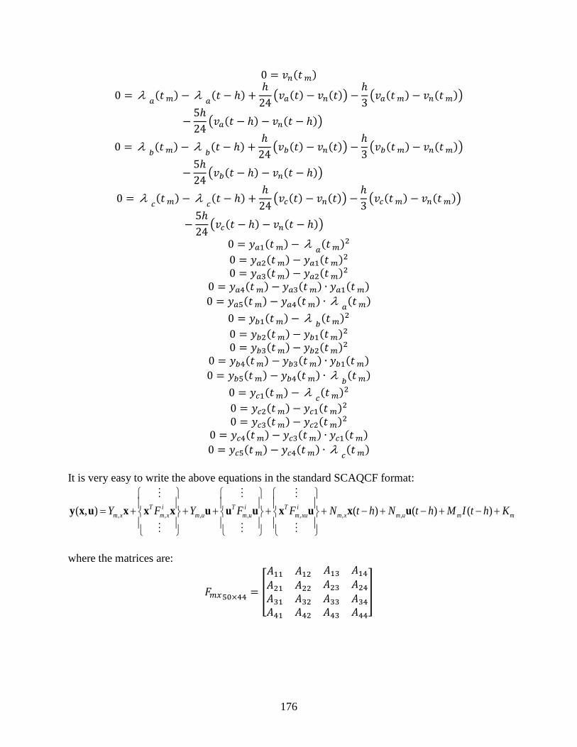
0 = 𝑣𝑣𝑛𝑛(𝑜𝑜 𝑚𝑚)

0 = λ 𝑚𝑚(𝑜𝑜 𝑚𝑚) − λ 𝑚𝑚(𝑜𝑜 − ℎ) +ℎ

24�𝑣𝑣𝑚𝑚(𝑜𝑜) − 𝑣𝑣𝑛𝑛(𝑜𝑜)� −

ℎ3�𝑣𝑣𝑚𝑚(𝑜𝑜 𝑚𝑚) − 𝑣𝑣𝑛𝑛(𝑜𝑜 𝑚𝑚)�

−5ℎ24

�𝑣𝑣𝑚𝑚(𝑜𝑜 − ℎ) − 𝑣𝑣𝑛𝑛(𝑜𝑜 − ℎ)�

0 = λ 𝑏𝑏(𝑜𝑜 𝑚𝑚) − λ 𝑏𝑏(𝑜𝑜 − ℎ) +ℎ

24�𝑣𝑣𝑏𝑏(𝑜𝑜) − 𝑣𝑣𝑛𝑛(𝑜𝑜)� −

ℎ3�𝑣𝑣𝑏𝑏(𝑜𝑜 𝑚𝑚) − 𝑣𝑣𝑛𝑛(𝑜𝑜 𝑚𝑚)�

−5ℎ24

�𝑣𝑣𝑏𝑏(𝑜𝑜 − ℎ) − 𝑣𝑣𝑛𝑛(𝑜𝑜 − ℎ)�

0 = λ 𝑐𝑐(𝑜𝑜 𝑚𝑚) − λ 𝑐𝑐(𝑜𝑜 − ℎ) +ℎ

24�𝑣𝑣𝑐𝑐(𝑜𝑜) − 𝑣𝑣𝑛𝑛(𝑜𝑜)� −

ℎ3�𝑣𝑣𝑐𝑐(𝑜𝑜 𝑚𝑚) − 𝑣𝑣𝑛𝑛(𝑜𝑜 𝑚𝑚)�

−5ℎ24

�𝑣𝑣𝑐𝑐(𝑜𝑜 − ℎ) − 𝑣𝑣𝑛𝑛(𝑜𝑜 − ℎ)�

0 = 𝑦𝑦𝑚𝑚1(𝑜𝑜 𝑚𝑚) − λ 𝑚𝑚(𝑜𝑜 𝑚𝑚)2 0 = 𝑦𝑦𝑚𝑚2(𝑜𝑜 𝑚𝑚) − 𝑦𝑦𝑚𝑚1(𝑜𝑜 𝑚𝑚)2 0 = 𝑦𝑦𝑚𝑚3(𝑜𝑜 𝑚𝑚) − 𝑦𝑦𝑚𝑚2(𝑜𝑜 𝑚𝑚)2

0 = 𝑦𝑦𝑚𝑚4(𝑜𝑜 𝑚𝑚) − 𝑦𝑦𝑚𝑚3(𝑜𝑜 𝑚𝑚) ∙ 𝑦𝑦𝑚𝑚1(𝑜𝑜 𝑚𝑚) 0 = 𝑦𝑦𝑚𝑚5(𝑜𝑜 𝑚𝑚) − 𝑦𝑦𝑚𝑚4(𝑜𝑜 𝑚𝑚) ∙ λ 𝑚𝑚(𝑜𝑜 𝑚𝑚)

0 = 𝑦𝑦𝑏𝑏1(𝑜𝑜 𝑚𝑚) − λ 𝑏𝑏(𝑜𝑜 𝑚𝑚)2 0 = 𝑦𝑦𝑏𝑏2(𝑜𝑜 𝑚𝑚) − 𝑦𝑦𝑏𝑏1(𝑜𝑜 𝑚𝑚)2 0 = 𝑦𝑦𝑏𝑏3(𝑜𝑜 𝑚𝑚) − 𝑦𝑦𝑏𝑏2(𝑜𝑜 𝑚𝑚)2

0 = 𝑦𝑦𝑏𝑏4(𝑜𝑜 𝑚𝑚) − 𝑦𝑦𝑏𝑏3(𝑜𝑜 𝑚𝑚) ∙ 𝑦𝑦𝑏𝑏1(𝑜𝑜 𝑚𝑚) 0 = 𝑦𝑦𝑏𝑏5(𝑜𝑜 𝑚𝑚) − 𝑦𝑦𝑏𝑏4(𝑜𝑜 𝑚𝑚) ∙ λ 𝑏𝑏(𝑜𝑜 𝑚𝑚)

0 = 𝑦𝑦𝑐𝑐1(𝑜𝑜 𝑚𝑚) − λ 𝑐𝑐(𝑜𝑜 𝑚𝑚)2 0 = 𝑦𝑦𝑐𝑐2(𝑜𝑜 𝑚𝑚) − 𝑦𝑦𝑐𝑐1(𝑜𝑜 𝑚𝑚)2 0 = 𝑦𝑦𝑐𝑐3(𝑜𝑜 𝑚𝑚) − 𝑦𝑦𝑐𝑐2(𝑜𝑜 𝑚𝑚)2

0 = 𝑦𝑦𝑐𝑐4(𝑜𝑜 𝑚𝑚) − 𝑦𝑦𝑐𝑐3(𝑜𝑜 𝑚𝑚) ∙ 𝑦𝑦𝑐𝑐1(𝑜𝑜 𝑚𝑚) 0 = 𝑦𝑦𝑐𝑐5(𝑜𝑜 𝑚𝑚) − 𝑦𝑦𝑐𝑐4(𝑜𝑜 𝑚𝑚) ∙ λ 𝑐𝑐(𝑜𝑜 𝑚𝑚)

It is very easy to write the above equations in the standard SCAQCF format:


= + + + + + − + − + − +



𝐹𝐹𝑚𝑚𝑒𝑒50×44 = �




�

176

( )11 10 7

1 0 0 0 0 00 1 0 0 0 00 0 1 0 0 0

0 0 0 0 00 0 0 0 00 0 0 0 0

0 0 0

0 0 1 0 06 6

0 0 0 1 06 6

0

111

0 0

0 0 0 16 6

0 1

L L

L L

L L

g gg g

g gA

h h

h h

h h

×

= −

−−−

−−

− −

−

( )

011

0

011

012 10 15

011

0

0 0 011 11 11

0 0 0

00 0 0 0 0 0 0 0 0 0 0 0 0 0

00 0 0 0 0 0 0 0 0 0 0 0 0 0

00 0 0 0 0 0 0 0 0 0 0 0 0 00 0 0 0 0 0 0 0 0 0 0 0 0 0

0 0 0 0 0 0 0 0 0 0 0 0 0 0

0 0 0 0 0 0 0 0 0 0 0 0 0 0

0 0 0 0 0 0 0 0 0 0 0 0

0 0 0 0 0 0 0 0 0 0 0 0 0 0 00 0 0 0 0 0 0 0 0 0 0 0 0 0 00 0 0 0 0 0 0 0 0 0 0 0 0 0 0

i

i

Ai

i i i

λ

λ

λ

λ λ λ

×

=

− − −

177

( )13 10 7

0 0 0 0 0 0 00 0 0 0 0 0 00 0 0 0 0 0 00 0 0 0 0 0 00 0 0 0 0 0 00 0 0 0 0 0 00 0 0 0 0 0 02 20 0 0 0 03 3

2 20 0 0 0 03 3

2 20 0 0 0 03 3

A

h h

h h

h h

×

= − − −

𝐴𝐴14 = [0]10×15

[ ]21 15 70A

×=

22 15 15A I ×= 𝐴𝐴23 = [0]15×7 𝐴𝐴24 = [0]15×15

( )31 10 7

0 0 0 0 0 0 00 0 0 0 0 0 00 0 0 0 0 0 00 0 0 0 0 0 00 0 0 0 0 0 00 0 0 0 0 0 00 0 0 0 0 0 0

0 0 0 0 024 24

0 0 0 0 024 24

0 0 0 0 024 24

A

h h

h h

h h

×

= − − −

𝐴𝐴32 = [0]7×15

178

( )33 10 7

1 0 0 0 0 00 1 0 0 0 00 0 1 0 0 0

0 0 0 0 00 0 0 0 00 0 0 0 0

0 0 0

0 0 1 0 03 3

0 0 0 1 03 3

0

111

0 0

0 0 0 13 3

0 1

L L

L L

L L

g gg g

g gA

h h

h h

h h

×

= −

−−−

−−

− −

−

( )

011

0

011

034 10 15

011

0

0 0 011 11 11

0 0 0

00 0 0 0 0 0 0 0 0 0 0 0 0 0

00 0 0 0 0 0 0 0 0 0 0 0 0 0

00 0 0 0 0 0 0 0 0 0 0 0 0 00 0 0 0 0 0 0 0 0 0 0 0 0 0

0 0 0 0 0 0 0 0 0 0 0 0 0 0

0 0 0 0 0 0 0 0 0 0 0 0 0 0

0 0 0 0 0 0 0 0 0 0 0 0

0 0 0 0 0 0 0 0 0 0 0 0 0 0 00 0 0 0 0 0 0 0 0 0 0 0 0 0 00 0 0 0 0 0 0 0 0 0 0 0 0 0 0

i

i

Ai

i i i

λ

λ

λ

λ λ λ

×

=

− − −

[ ]41 15 70A

×=

42 15 15[0]A ×= 𝐴𝐴43 = [0]15×7 𝐴𝐴44 = 𝐼𝐼15×15

𝐹𝐹𝑚𝑚𝑒𝑒0 = ⋯ = 𝐹𝐹𝑚𝑚𝑒𝑒9 = 044×44 𝐹𝐹𝑚𝑚𝑒𝑒10: 𝑓𝑓𝑚𝑚𝑒𝑒[5×5] = −1, 𝑜𝑜𝑜𝑜ℎ𝑒𝑒𝑒𝑒 𝑒𝑒𝑒𝑒𝑒𝑒𝑒𝑒𝑒𝑒𝑒𝑒𝑜𝑜𝑒𝑒 𝑎𝑎𝑒𝑒𝑒𝑒 0 𝐹𝐹𝑚𝑚𝑒𝑒11: 𝑓𝑓𝑚𝑚𝑒𝑒[8×8] = −1, 𝑜𝑜𝑜𝑜ℎ𝑒𝑒𝑒𝑒 𝑒𝑒𝑒𝑒𝑒𝑒𝑒𝑒𝑒𝑒𝑒𝑒𝑜𝑜𝑒𝑒 𝑎𝑎𝑒𝑒𝑒𝑒 0 𝐹𝐹𝑚𝑚𝑒𝑒12: 𝑓𝑓𝑚𝑚𝑒𝑒[9×9] = −1, 𝑜𝑜𝑜𝑜ℎ𝑒𝑒𝑒𝑒 𝑒𝑒𝑒𝑒𝑒𝑒𝑒𝑒𝑒𝑒𝑒𝑒𝑜𝑜𝑒𝑒 𝑎𝑎𝑒𝑒𝑒𝑒 0

179

𝐹𝐹𝑚𝑚𝑒𝑒13: 𝑓𝑓𝑚𝑚𝑒𝑒[10×8] = −1, 𝑜𝑜𝑜𝑜ℎ𝑒𝑒𝑒𝑒 𝑒𝑒𝑒𝑒𝑒𝑒𝑒𝑒𝑒𝑒𝑒𝑒𝑜𝑜𝑒𝑒 𝑎𝑎𝑒𝑒𝑒𝑒 0 𝐹𝐹𝑚𝑚𝑒𝑒14: 𝑓𝑓𝑚𝑚𝑒𝑒[11×5] = −1, 𝑜𝑜𝑜𝑜ℎ𝑒𝑒𝑒𝑒 𝑒𝑒𝑒𝑒𝑒𝑒𝑒𝑒𝑒𝑒𝑒𝑒𝑜𝑜𝑒𝑒 𝑎𝑎𝑒𝑒𝑒𝑒 0 𝐹𝐹𝑚𝑚𝑒𝑒15: 𝑓𝑓𝑚𝑚𝑒𝑒[6×6] = −1, 𝑜𝑜𝑜𝑜ℎ𝑒𝑒𝑒𝑒 𝑒𝑒𝑒𝑒𝑒𝑒𝑒𝑒𝑒𝑒𝑒𝑒𝑜𝑜𝑒𝑒 𝑎𝑎𝑒𝑒𝑒𝑒 0 𝐹𝐹𝑚𝑚𝑒𝑒16: 𝑓𝑓𝑚𝑚𝑒𝑒[13×13] = −1, 𝑜𝑜𝑜𝑜ℎ𝑒𝑒𝑒𝑒 𝑒𝑒𝑒𝑒𝑒𝑒𝑒𝑒𝑒𝑒𝑒𝑒𝑜𝑜𝑒𝑒 𝑎𝑎𝑒𝑒𝑒𝑒 0 𝐹𝐹𝑚𝑚𝑒𝑒17: 𝑓𝑓𝑚𝑚𝑒𝑒[14×14] = −1, 𝑜𝑜𝑜𝑜ℎ𝑒𝑒𝑒𝑒 𝑒𝑒𝑒𝑒𝑒𝑒𝑒𝑒𝑒𝑒𝑒𝑒𝑜𝑜𝑒𝑒 𝑎𝑎𝑒𝑒𝑒𝑒 0 𝐹𝐹𝑚𝑚𝑒𝑒18: 𝑓𝑓𝑚𝑚𝑒𝑒[15×13] = −1, 𝑜𝑜𝑜𝑜ℎ𝑒𝑒𝑒𝑒 𝑒𝑒𝑒𝑒𝑒𝑒𝑒𝑒𝑒𝑒𝑒𝑒𝑜𝑜𝑒𝑒 𝑎𝑎𝑒𝑒𝑒𝑒 0 𝐹𝐹𝑚𝑚𝑒𝑒19: 𝑓𝑓𝑚𝑚𝑒𝑒[16×6] = −1, 𝑜𝑜𝑜𝑜ℎ𝑒𝑒𝑒𝑒 𝑒𝑒𝑒𝑒𝑒𝑒𝑒𝑒𝑒𝑒𝑒𝑒𝑜𝑜𝑒𝑒 𝑎𝑎𝑒𝑒𝑒𝑒 0 𝐹𝐹𝑚𝑚𝑒𝑒20: 𝑓𝑓𝑚𝑚𝑒𝑒[7×7] = −1, 𝑜𝑜𝑜𝑜ℎ𝑒𝑒𝑒𝑒 𝑒𝑒𝑒𝑒𝑒𝑒𝑒𝑒𝑒𝑒𝑒𝑒𝑜𝑜𝑒𝑒 𝑎𝑎𝑒𝑒𝑒𝑒 0 𝐹𝐹𝑚𝑚𝑒𝑒21: 𝑓𝑓𝑚𝑚𝑒𝑒[18×18] = −1, 𝑜𝑜𝑜𝑜ℎ𝑒𝑒𝑒𝑒 𝑒𝑒𝑒𝑒𝑒𝑒𝑒𝑒𝑒𝑒𝑒𝑒𝑜𝑜𝑒𝑒 𝑎𝑎𝑒𝑒𝑒𝑒 0 𝐹𝐹𝑚𝑚𝑒𝑒22: 𝑓𝑓𝑚𝑚𝑒𝑒[19×19] = −1, 𝑜𝑜𝑜𝑜ℎ𝑒𝑒𝑒𝑒 𝑒𝑒𝑒𝑒𝑒𝑒𝑒𝑒𝑒𝑒𝑒𝑒𝑜𝑜𝑒𝑒 𝑎𝑎𝑒𝑒𝑒𝑒 0 𝐹𝐹𝑚𝑚𝑒𝑒23: 𝑓𝑓𝑚𝑚𝑒𝑒[20×18] = −1, 𝑜𝑜𝑜𝑜ℎ𝑒𝑒𝑒𝑒 𝑒𝑒𝑒𝑒𝑒𝑒𝑒𝑒𝑒𝑒𝑒𝑒𝑜𝑜𝑒𝑒 𝑎𝑎𝑒𝑒𝑒𝑒 0 𝐹𝐹𝑚𝑚𝑒𝑒24: 𝑓𝑓𝑚𝑚𝑒𝑒[21×7] = −1, 𝑜𝑜𝑜𝑜ℎ𝑒𝑒𝑒𝑒 𝑒𝑒𝑒𝑒𝑒𝑒𝑒𝑒𝑒𝑒𝑒𝑒𝑜𝑜𝑒𝑒 𝑎𝑎𝑒𝑒𝑒𝑒 0

𝐹𝐹𝑚𝑚𝑒𝑒25 = ⋯ = 𝐹𝐹𝑚𝑚𝑒𝑒34 = 044×44

𝐹𝐹𝑚𝑚𝑒𝑒35: 𝑓𝑓𝑚𝑚𝑒𝑒[27×27] = −1, 𝑜𝑜𝑜𝑜ℎ𝑒𝑒𝑒𝑒 𝑒𝑒𝑒𝑒𝑒𝑒𝑒𝑒𝑒𝑒𝑒𝑒𝑜𝑜𝑒𝑒 𝑎𝑎𝑒𝑒𝑒𝑒 0 𝐹𝐹𝑚𝑚𝑒𝑒36: 𝑓𝑓𝑚𝑚𝑒𝑒[30×30] = −1, 𝑜𝑜𝑜𝑜ℎ𝑒𝑒𝑒𝑒 𝑒𝑒𝑒𝑒𝑒𝑒𝑒𝑒𝑒𝑒𝑒𝑒𝑜𝑜𝑒𝑒 𝑎𝑎𝑒𝑒𝑒𝑒 0 𝐹𝐹𝑚𝑚𝑒𝑒37: 𝑓𝑓𝑚𝑚𝑒𝑒[31×31] = −1, 𝑜𝑜𝑜𝑜ℎ𝑒𝑒𝑒𝑒 𝑒𝑒𝑒𝑒𝑒𝑒𝑒𝑒𝑒𝑒𝑒𝑒𝑜𝑜𝑒𝑒 𝑎𝑎𝑒𝑒𝑒𝑒 0 𝐹𝐹𝑚𝑚𝑒𝑒38: 𝑓𝑓𝑚𝑚𝑒𝑒[32×30] = −1, 𝑜𝑜𝑜𝑜ℎ𝑒𝑒𝑒𝑒 𝑒𝑒𝑒𝑒𝑒𝑒𝑒𝑒𝑒𝑒𝑒𝑒𝑜𝑜𝑒𝑒 𝑎𝑎𝑒𝑒𝑒𝑒 0 𝐹𝐹𝑚𝑚𝑒𝑒39: 𝑓𝑓𝑚𝑚𝑒𝑒[33×27] = −1, 𝑜𝑜𝑜𝑜ℎ𝑒𝑒𝑒𝑒 𝑒𝑒𝑒𝑒𝑒𝑒𝑒𝑒𝑒𝑒𝑒𝑒𝑜𝑜𝑒𝑒 𝑎𝑎𝑒𝑒𝑒𝑒 0 𝐹𝐹𝑚𝑚𝑒𝑒40: 𝑓𝑓𝑚𝑚𝑒𝑒[28×28] = −1, 𝑜𝑜𝑜𝑜ℎ𝑒𝑒𝑒𝑒 𝑒𝑒𝑒𝑒𝑒𝑒𝑒𝑒𝑒𝑒𝑒𝑒𝑜𝑜𝑒𝑒 𝑎𝑎𝑒𝑒𝑒𝑒 0 𝐹𝐹𝑚𝑚𝑒𝑒41: 𝑓𝑓𝑚𝑚𝑒𝑒[35×35] = −1, 𝑜𝑜𝑜𝑜ℎ𝑒𝑒𝑒𝑒 𝑒𝑒𝑒𝑒𝑒𝑒𝑒𝑒𝑒𝑒𝑒𝑒𝑜𝑜𝑒𝑒 𝑎𝑎𝑒𝑒𝑒𝑒 0 𝐹𝐹𝑚𝑚𝑒𝑒42: 𝑓𝑓𝑚𝑚𝑒𝑒[36×36] = −1, 𝑜𝑜𝑜𝑜ℎ𝑒𝑒𝑒𝑒 𝑒𝑒𝑒𝑒𝑒𝑒𝑒𝑒𝑒𝑒𝑒𝑒𝑜𝑜𝑒𝑒 𝑎𝑎𝑒𝑒𝑒𝑒 0 𝐹𝐹𝑚𝑚𝑒𝑒43: 𝑓𝑓𝑚𝑚𝑒𝑒[37×35] = −1, 𝑜𝑜𝑜𝑜ℎ𝑒𝑒𝑒𝑒 𝑒𝑒𝑒𝑒𝑒𝑒𝑒𝑒𝑒𝑒𝑒𝑒𝑜𝑜𝑒𝑒 𝑎𝑎𝑒𝑒𝑒𝑒 0 𝐹𝐹𝑚𝑚𝑒𝑒44: 𝑓𝑓𝑚𝑚𝑒𝑒[38×28] = −1, 𝑜𝑜𝑜𝑜ℎ𝑒𝑒𝑒𝑒 𝑒𝑒𝑒𝑒𝑒𝑒𝑒𝑒𝑒𝑒𝑒𝑒𝑜𝑜𝑒𝑒 𝑎𝑎𝑒𝑒𝑒𝑒 0 𝐹𝐹𝑚𝑚𝑒𝑒45: 𝑓𝑓𝑚𝑚𝑒𝑒[29×29] = −1, 𝑜𝑜𝑜𝑜ℎ𝑒𝑒𝑒𝑒 𝑒𝑒𝑒𝑒𝑒𝑒𝑒𝑒𝑒𝑒𝑒𝑒𝑜𝑜𝑒𝑒 𝑎𝑎𝑒𝑒𝑒𝑒 0 𝐹𝐹𝑚𝑚𝑒𝑒46: 𝑓𝑓𝑚𝑚𝑒𝑒[40×40] = −1, 𝑜𝑜𝑜𝑜ℎ𝑒𝑒𝑒𝑒 𝑒𝑒𝑒𝑒𝑒𝑒𝑒𝑒𝑒𝑒𝑒𝑒𝑜𝑜𝑒𝑒 𝑎𝑎𝑒𝑒𝑒𝑒 0 𝐹𝐹𝑚𝑚𝑒𝑒47: 𝑓𝑓𝑚𝑚𝑒𝑒[41×41] = −1, 𝑜𝑜𝑜𝑜ℎ𝑒𝑒𝑒𝑒 𝑒𝑒𝑒𝑒𝑒𝑒𝑒𝑒𝑒𝑒𝑒𝑒𝑜𝑜𝑒𝑒 𝑎𝑎𝑒𝑒𝑒𝑒 0 𝐹𝐹𝑚𝑚𝑒𝑒348: 𝑓𝑓𝑚𝑚𝑒𝑒[42×40] = −1, 𝑜𝑜𝑜𝑜ℎ𝑒𝑒𝑒𝑒 𝑒𝑒𝑒𝑒𝑒𝑒𝑒𝑒𝑒𝑒𝑒𝑒𝑜𝑜𝑒𝑒 𝑎𝑎𝑒𝑒𝑒𝑒 0 𝐹𝐹𝑚𝑚𝑒𝑒49: 𝑓𝑓𝑚𝑚𝑒𝑒[43×29] = −1, 𝑜𝑜𝑜𝑜ℎ𝑒𝑒𝑒𝑒 𝑒𝑒𝑒𝑒𝑒𝑒𝑒𝑒𝑒𝑒𝑒𝑒𝑜𝑜𝑒𝑒 𝑎𝑎𝑒𝑒𝑒𝑒 0

𝑁𝑁𝑚𝑚𝑒𝑒50𝑋𝑋7 =

⎣⎢⎢⎢⎡

07𝑋𝑋7𝐵𝐵1(3𝑋𝑋7)022𝑋𝑋7𝐵𝐵2(3𝑋𝑋7)015𝑋𝑋7 ⎦

⎥⎥⎥⎤

1

0 0 1 0 06 6

0 0 0 1 06 6

0 0 0 0 16 6

h h

h hB

h h

− − = − − − −

180

2

5 50 0 1 0 024 24

5 50 0 0 1 024 24

5 50 0 0 0 124 24

h h

h hB

h h

− − = − − − −

181

Setting-less Protection: Laboratory Testing · Setting-less Protection: ... Application to Three...

Documents

Transcript of Setting-less Protection: Laboratory Testing · Setting-less Protection: ... Application to Three...