Set Theory - Computer Science Department - Stony Brook University
2
Syllabus
• Mathematical argument: Basic mathematical notation and argument, in-cluding proof by contradiction, mathematical induction and its variants.
• Sets and logic: Subsets of a fixed set as a Boolean algebra. Venn diagrams.Propositional logic and its models. Validity, entailment, and equivalence ofboolean propositions. Truth tables. Structural induction. Simplificationof boolean propositions and set expressions.
• Relations and functions: Product of sets. Relations, functions and partialfunctions. Composition and identity relations. Injective, surjective andbijective functions. Direct and inverse image of a set under a relation.Equivalence relations and partitions. Directed graphs and partial orders.Size of sets, especially countability. Cantor’s diagonal argument to showthe reals are uncountable.
• Constructions on sets: Russell’s paradox. Basic sets, comprehension, in-dexed sets, unions, intersections, products, disjoint unions, powersets.Characteristic functions. Sets of functions. Lambda notation for func-tions. Cantor’s diagonal argument to show powerset strictly increases size.An informal presentation of the axioms of Zermelo-Fraenkel set theory andthe axiom of choice.
• Inductive definitions: Using rules to define sets. Reasoning principles:rule induction and its instances; induction on derivations. Applications,including transitive closure of a relation. Inductive definitions as leastfixed points. Tarski’s fixed point theorem for monotonic functions on apowerset. Maximum fixed points and coinduction.
• Well-founded induction: Well-founded relations and well-founded induc-tion. Examples. Constructing well-founded relations, including productand lexicographic product of well-founded relations. Applications. Well-founded recursion.
• Inductively-defined properties and classes: Ordinals and transfinite induc-tion.
• Fraenkel-Mostowski sets: Failure of the axiom of choice in Fraenkel-Mostowskisets. Freshness. Nominal sets.
Aims and objectives
The aim is to introduce fundamental concepts and techniques in set theory inpreparation for its many applications in computer science. On completing thiscourse, students should be able to
• understand and be able to use the language of set theory; prove anddisprove assertions using a variety of techniques.
3
• understand the formalization of basic logic (validity, entailment and truth)in set theory.
• define sets inductively using rules, formulate corresponding proof princi-ples, and prove properties about inductively-defined sets.
• understand Tarski’s fixed point theorem and the proof principles associ-ated with the least and greatest fixed points of monotonic functions on apowerset.
• understand and apply the principle of well-founded induction, includingtransfinite induction on the ordinals.
• have a basic understanding of Fraenkel-Mostowski sets and their proper-ties.
A brief history of sets
A set is an unordered collection of objects, and as such a set is determined bythe objects it contains. Before the 19th century it was uncommon to think ofsets as completed objects in their own right. Mathematicians were familiar withproperties such as being a natural number, or being irrational, but it was rare tothink of say the collection of rational numbers as itself an object. (There wereexceptions. From Euclid mathematicians were used to thinking of geometricobjects such as lines and planes and spheres which we might today identifywith their sets of points.)
In the mid 19th century there was a renaissance in Logic. For thousandsof years, since the time of Aristotle and before, learned individuals had beenfamiliar with syllogisms as patterns of legitimate reasoning, for example:
All men are mortal. Socrates is a man. Therefore Socrates is mortal.
But syllogisms involved descriptions of properties. The idea of pioneers such asBoole was to assign a meaning as a set to these descriptions. For example, thetwo descriptions “is a man” and “is a male homo sapiens” both describe thesame set, viz. the set of all men. It was this objectification of meaning, under-standing properties as sets, that led to a rebirth of Logic and Mathematics inthe 19th century. Cantor took the idea of set to a revolutionary level, unveilingits true power. By inventing a notion of size of set he was able compare dif-ferent forms of infinity and, almost incidentally, to shortcut several traditionalmathematical arguments.
But the power of sets came at a price; it came with dangerous paradoxes.The work of Boole and others suggested a programme exposited by Frege, andRussell and Whitehead, to build a foundation for all of Mathematics on Logic.Though to be more accurate, they were really reinventing Logic in the process,and regarding it as intimately bound up with a theory of sets. The paradoxesof set theory were a real threat to the security of the foundations. But witha lot of worry and care the paradoxes were sidestepped, first by Russell and
4
Whitehead’s theory of stratified types and then more elegantly, in for exam-ple the influential work of Zermelo and Fraenkel. The notion of set is now acornerstone of Mathematics.
The precise notion of proof present in the work of Russell and Whitehead laidthe scene for Godel’s astounding result of 1931: any sound proof system able todeal with arithmetic will necessarily be incomplete, in the sense that it will beimpossible to prove all the statements within the system which are true. Godel’stheorem relied on the mechanical nature of proof in order to be able to encodeproofs back into the proof system itself. After a flurry of activity, through thework of Godel himself, Church, Turing and others, it was realised by the mid1930’s that Godel’s incompleteness result rested on a fundamental notion, thatof computability. Arguably this marks the birth of Computer Science.
Motivation
Why learn Set Theory? Set Theory is an important language and tool forreasoning. It’s a basis for Mathematics—pretty much all Mathematics can beformalised in Set Theory.
Why is Set Theory important for Computer Science? It’s a useful tool forformalising and reasoning about computation and the objects of computation.Set Theory is indivisible from Logic where Computer Science has its roots.It has been and is likely to continue to be a a source of fundamental ideas inComputer Science from theory to practice; Computer Science, being a science ofthe artificial, has had many of its constructs and ideas inspired by Set Theory.The strong tradition, universality and neutrality of Set Theory make it firmcommon ground on which to provide unification between seemingly disparateareas and notations of Computer Science. Set Theory is likely to be aroundlong after most present-day programming languages have faded from memory.A knowledge of Set Theory should facilitate your ability to think abstractly. Itwill provide you with a foundation on which to build a firm understanding andanalysis of the new ideas in Computer Science that you will meet.
The art of proof
Proof is the activity of discovering and confirming truth. Proofs in mathematicsare not so far removed from coherent logical arguments of an everyday kind, ofthe sort a straight-thinking lawyer or politician might apply—an Obama, nota Bush! A main aim of this course and its attendant seminars is to help youharness that everyday facility to write down proofs which communicate well toother people. Here there’s an art in getting the balance right: too much detailand you can’t see the wood for the trees; too little and it’s hard to fill in thegaps. This course is not about teaching you how to do very formal proofs withina formal logical system, of the kind acceptable to machine verification—that’san important topic in itself, and one which we will touch on peripherally.
In Italy it’s said that it requires two people to make a good salad dressing;a generous person to add the oil and a mean person the vinegar. Constructing
5
proofs in mathematics is similar. Often a tolerant openness and awareness is im-portant in discovering or understanding a proof, while a strictness and disciplineis needed in writing it down. There are many different styles of thinking, evenamongst professional mathematicians, yet they can communicate well throughthe common medium of written proof. It’s important not to confuse the rigourof a well-written-down proof with the human and very individual activity ofgoing about discovering it or understanding it. Too much of a straightjacket onyour thinking is likely to stymie anything but the simplest proofs. On the otherhand too little discipline, and writing down too little on the way to a proof, canleave you uncertain and lost. When you cannot see a proof immediately (thismay happen most of the time initially), it can help to write down the assump-tions and the goal. Often starting to write down a proof helps you discoverit. You may have already experienced this in carrying out proofs by induction.It can happen that the induction hypothesis one starts out with isn’t strongenough to get the induction step. But starting to do the proof even with the‘wrong’ induction hypothesis can help you spot how to strengthen it.
Of course, there’s no better way to learn the art of proof than by doing proofs,no better way to read and understand a proof than to pause occasionally andtry to continue the proof yourself. For this reason you are encouraged to do theexercises—most of them are placed strategically in the appropriate place in thetext.Additional reading: The notes are self-contained. The more set-theory ori-ented books below are those of Devlin, Nissanke and Stanat-McAllister. Onlinesources such as Wikipedia can also be helpful.
Devlin, K. (2003) Sets, Functions, and Logic, An Introduction to Abstract Math-ematics. Chapman & Hall/CRC Mathematics (3rd ed.).Biggs, N.L. (1989). Discrete mathematics. Oxford University Press.Mattson, H.F. Jr (1993). Discrete mathematics. Wiley.Nissanke, N. (1999). Introductory logic and sets for computer scientists. Addison-Wesley.Polya, G. (1980). How to solve it. Penguin.Stanat, D.F., and McAllister, D.F. (1977), Discrete Mathematics in ComputerScience.Prentice-Hall.
Acknowledgements: To Hasan Amjad, Katy Edgcombe, Marcelo Fiore, ThomasForster, Ian Grant, Martin Hyland, Frank King, Ken Moody, Alan Mycroft,Andy Pitts, Peter Robinson, Sam Staton, Dave Turner for helpful suggestions.

6
Contents
1 Mathematical argument 111.1 Logical notation . . . . . . . . . . . . . . . . . . . . . . . . . . . 111.2 Patterns of proof . . . . . . . . . . . . . . . . . . . . . . . . . . . 13
1.2.1 Chains of implications . . . . . . . . . . . . . . . . . . . . 131.2.2 Proof by contradiction . . . . . . . . . . . . . . . . . . . . 131.2.3 Argument by cases . . . . . . . . . . . . . . . . . . . . . . 141.2.4 Existential properties . . . . . . . . . . . . . . . . . . . . 151.2.5 Universal properties . . . . . . . . . . . . . . . . . . . . . 15
1.3 Mathematical induction . . . . . . . . . . . . . . . . . . . . . . . 15
2 Sets and Logic 252.1 Sets . . . . . . . . . . . . . . . . . . . . . . . . . . . . . . . . . . 252.2 Set laws . . . . . . . . . . . . . . . . . . . . . . . . . . . . . . . . 26
2.2.1 The Boolean algebra of sets . . . . . . . . . . . . . . . . . 262.2.2 Venn diagrams . . . . . . . . . . . . . . . . . . . . . . . . 302.2.3 Boolean algebra and properties . . . . . . . . . . . . . . . 32
2.3 Propositional logic . . . . . . . . . . . . . . . . . . . . . . . . . . 322.3.1 Boolean propositions . . . . . . . . . . . . . . . . . . . . . 322.3.2 Models . . . . . . . . . . . . . . . . . . . . . . . . . . . . 342.3.3 Truth assignments . . . . . . . . . . . . . . . . . . . . . . 372.3.4 Truth tables . . . . . . . . . . . . . . . . . . . . . . . . . . 402.3.5 Methods . . . . . . . . . . . . . . . . . . . . . . . . . . . . 42
3 Relations and functions 453.1 Ordered pairs and products . . . . . . . . . . . . . . . . . . . . . 453.2 Relations and functions . . . . . . . . . . . . . . . . . . . . . . . 46
3.2.1 Composing relations and functions . . . . . . . . . . . . . 473.2.2 Direct and inverse image under a relation . . . . . . . . . 49
3.3 Relations as structure . . . . . . . . . . . . . . . . . . . . . . . . 503.3.1 Directed graphs . . . . . . . . . . . . . . . . . . . . . . . . 503.3.2 Equivalence relations . . . . . . . . . . . . . . . . . . . . . 503.3.3 Partial orders . . . . . . . . . . . . . . . . . . . . . . . . . 53
3.4 Size of sets . . . . . . . . . . . . . . . . . . . . . . . . . . . . . . 553.4.1 Countability . . . . . . . . . . . . . . . . . . . . . . . . . 55
7
8 CONTENTS
3.4.2 Uncountability . . . . . . . . . . . . . . . . . . . . . . . . 59
4 Constructions on sets 634.1 Russell’s paradox . . . . . . . . . . . . . . . . . . . . . . . . . . . 634.2 Constructing sets . . . . . . . . . . . . . . . . . . . . . . . . . . . 64
4.2.1 Basic sets . . . . . . . . . . . . . . . . . . . . . . . . . . . 644.2.2 Constructions . . . . . . . . . . . . . . . . . . . . . . . . . 644.2.3 Axioms of set theory . . . . . . . . . . . . . . . . . . . . . 68
4.3 Some consequences . . . . . . . . . . . . . . . . . . . . . . . . . . 694.3.1 Sets of functions . . . . . . . . . . . . . . . . . . . . . . . 694.3.2 Sets of unlimited size . . . . . . . . . . . . . . . . . . . . . 71
5 Inductive definitions 735.1 Sets defined by rules—examples . . . . . . . . . . . . . . . . . . . 735.2 Inductively-defined sets . . . . . . . . . . . . . . . . . . . . . . . 775.3 Rule induction . . . . . . . . . . . . . . . . . . . . . . . . . . . . 78
5.3.1 Transitive closure of a relation . . . . . . . . . . . . . . . 825.4 Derivation trees . . . . . . . . . . . . . . . . . . . . . . . . . . . . 835.5 Least fixed points . . . . . . . . . . . . . . . . . . . . . . . . . . . 865.6 Tarski’s fixed point theorem . . . . . . . . . . . . . . . . . . . . . 88
6 Well-founded induction 916.1 Well-founded relations . . . . . . . . . . . . . . . . . . . . . . . . 916.2 Well-founded induction . . . . . . . . . . . . . . . . . . . . . . . . 926.3 Building well-founded relations . . . . . . . . . . . . . . . . . . . 94
6.3.1 Fundamental well-founded relations . . . . . . . . . . . . 946.3.2 Transitive closure . . . . . . . . . . . . . . . . . . . . . . . 946.3.3 Product . . . . . . . . . . . . . . . . . . . . . . . . . . . . 946.3.4 Lexicographic products . . . . . . . . . . . . . . . . . . . 956.3.5 Inverse image . . . . . . . . . . . . . . . . . . . . . . . . . 96
6.4 Applications . . . . . . . . . . . . . . . . . . . . . . . . . . . . . . 966.4.1 Euclid’s algorithm for hcf . . . . . . . . . . . . . . . . . . 966.4.2 Eulerian graphs . . . . . . . . . . . . . . . . . . . . . . . . 986.4.3 Ackermann’s function . . . . . . . . . . . . . . . . . . . . 99
6.5 Well-founded recursion . . . . . . . . . . . . . . . . . . . . . . . . 1016.5.1 The proof of well-founded recursion . . . . . . . . . . . . 103
7 Inductively-defined classes 1057.1 Sets, properties and classes . . . . . . . . . . . . . . . . . . . . . 1057.2 Inductively-defined properties and classes . . . . . . . . . . . . . 1067.3 Induction principles for inductively-defined classes . . . . . . . . 1077.4 Ordinals . . . . . . . . . . . . . . . . . . . . . . . . . . . . . . . . 107
7.4.1 Properties of ordinals . . . . . . . . . . . . . . . . . . . . 1097.4.2 The Burali-Forti paradox . . . . . . . . . . . . . . . . . . 1107.4.3 Transfinite induction and recursion . . . . . . . . . . . . . 1117.4.4 Cardinals as ordinals . . . . . . . . . . . . . . . . . . . . . 112
CONTENTS 9
7.4.5 Tarski’s fixed point theorem revisited . . . . . . . . . . . 1137.5 The cumulative hierarchy . . . . . . . . . . . . . . . . . . . . . . 115
8 Fraenkel-Mostowski sets 1178.1 Atoms and permutations . . . . . . . . . . . . . . . . . . . . . . . 1178.2 Classes with an action . . . . . . . . . . . . . . . . . . . . . . . . 1188.3 Fraenkel-Mostowski sets . . . . . . . . . . . . . . . . . . . . . . . 1198.4 Constructions on FM sets . . . . . . . . . . . . . . . . . . . . . . 121
8.4.1 Failure of the axiom of choice in FM sets . . . . . . . . . 1228.5 Freshness . . . . . . . . . . . . . . . . . . . . . . . . . . . . . . . 1228.6 Nominal sets . . . . . . . . . . . . . . . . . . . . . . . . . . . . . 126
8.6.1 Nominal sets and equivariant functions . . . . . . . . . . . 1268.6.2 α-equivalence and atom abstraction . . . . . . . . . . . . 127
9 Exercises 131

10 CONTENTS
Chapter 1
Mathematical argument
Basic mathematical notation and methods of argument are introduced, includ-ing a review of the important principle of mathematical induction.
1.1 Logical notation
We shall use some informal logical notation in order to stop our mathematicalstatements getting out of hand. For statements (or assertions) A and B, weshall commonly use abbreviations like:
• A & B for (A and B), the conjunction of A and B,
• A⇒ B for (A implies B), which means (if A then B), and so is automat-ically true when A is false,
• A ⇐⇒ B to mean (A iff B), which abbreviates (A if and only if B), andexpresses the logical equivalence of A and B.
We shall also make statements by forming disjunctions (A or B), with the self-evident meaning, and negations (not A), sometimes written ¬A, which is trueiff A is false. There is a tradition to write for instance 7 6< 5 instead of ¬(7 < 5),which reflects what we generally say: “7 is not less than 5” rather than “not 7is less than 5.”
The statements may contain variables (or unknowns, or place-holders), as in
(x ≤ 3) & (y ≤ 7)
which is true when the variables x and y over integers stand for integers less thanor equal to 3 and 7 respectively, and false otherwise. A statement like P (x, y),which involves variables x, y, is called a predicate (or property, or relation,or condition) and it only becomes true or false when the pair x, y stand forparticular things.
11
12 CHAPTER 1. MATHEMATICAL ARGUMENT
We use logical quantifiers ∃, read “there exists”, and ∀, read “ for all”. Thenyou can read assertions like
∃x. P (x)
as abbreviating “for some x, P (x)” or “there exists x such that P (x)”, and
∀x. P (x)
as abbreviating “ for all x, P (x)” or “for any x, P (x)”. The statement
∃x, y, · · · , z. P (x, y, · · · , z)
abbreviates∃x∃y · · · ∃z. P (x, y, · · · , z),
and∀x, y, · · · , z. P (x, y, · · · , z)
abbreviates∀x∀y · · · ∀z. P (x, y, · · · , z).
Sometimes you’ll see a range for the quantification given explicitly as in∀x (0 < x ≤ k). P (x). Later, we often wish to specify a set X over whicha quantified variable ranges. Then one writes ∀x ∈ X. P (x)—read “for all xin X, P (x)”— instead of ∀x. x ∈ X ⇒ P (x), and ∃x ∈ X. P (x) instead of∃x. x ∈ X & P (x).
There is another useful notation associated with quantifiers. Occasionallyone wants to say not just that there exists some x satisfying a property P (x)but also that x is the unique object satisfying P (x). It is traditional to write
∃!x. P (x)
as an abbreviation for
(∃x. P (x)) & (∀y, z. P (y) & P (z)⇒ y = z)
which means that there is some x satisfying the property P (x) and also thatif any y, z both satisfy the property they are equal. This expresses that thereexists a unique x satisfying P (x).
Occasionally, and largely for abbreviation, we will write e.g., X =def Eto mean that X is defined to be E. Similarly, we will sometimes use e.g.,P (x)⇔def A in defining a property in terms of an expression A.
Exercise 1.1 What is the difference between ∀x.(∃y.P (x, y)) and ∃y.(∀x.P (x, y))?[You might like to consider P (x, y) to mean “x loves y.”] 2
1.2. PATTERNS OF PROOF 13
1.2 Patterns of proof
There is no magic formula for discovering proofs in anything but the simplestcontexts. However often the initial understanding of a problem suggests a gen-eral pattern of proof. Patterns of proof like those below appear frequently, oftenlocally as ingredients of a bigger proof, and are often amongst the first thingsto try. It is perhaps best to tackle this section fairly quickly at a first reading,and revisit it later when you have had more experience in doing proofs.
1.2.1 Chains of implications
To prove an A⇒ B it suffices to show that starting from the assumption A onecan prove B. Often a proof of A⇒ B factors into a chain of implications, eachone a manageable step:
A⇒ A1
⇒ · · ·⇒ An
⇒ B .
This really stands for
A⇒ A1, A1 ⇒ A2, · · · , An ⇒ B .
One can just as well write “Therefore” (or “∴”) between the different lines, andthis is preferable if the assertions A1, · · · , An are large.
A logical equivalence A ⇐⇒ B stands for both A ⇒ B and B ⇒ A. Oneoften sees a proof of a logical equivalence A ⇐⇒ B broken down into a chain
A ⇐⇒ A1
⇐⇒ · · ·⇐⇒ An
⇐⇒ B .
A common mistake is not to check the equivalence in the backwards direction, sothat while the implication Ai−1 to Ai is obvious enough, the reverse implicationfrom Ai to Ai−1 is unclear, in which case an explanation is needed, or evenuntrue. Remember, while a proof of A ⇐⇒ B very often does factor into aproof of A ⇒ B and B ⇒ A, the proof route taken in showing B ⇒ A needn’tbe the reverse of that taken in showing A⇒ B.
1.2.2 Proof by contradiction
The method of proof by contradiction was known to the ancients and carriesthe Latin name reductio ad absurdum. Sometimes the only known proof of anassertion A is by contradiction. In a proof by contradiction, to show A, oneshows that assuming ¬A leads to a conclusion which is false. We have thusshown ¬A is not the case, so A.
14 CHAPTER 1. MATHEMATICAL ARGUMENT
That√
2 is irrational was a dreadful secret known to the followers of Pythago-ras. The proof is a proof by contradiction: Assume, with the aim of obtaining acontradiction, that
√2 is rational, i.e.
√2 = a/b where a and b are integers with
no common prime factors. Then, 2b2 = a2. Therefore 2 divides a, so a = 2a0
for some integer a0. But then b2 = 2a20. So 2 also divides b—a contradiction.
Beware: a “beginner’s mistake” is an infatuation with proof by contradiction,leading to its use even when a direct proof is at least as easy.
Exercise 1.2 Show for any integer m that√m is rational iff m is a square, i.e.
m = a2 for some integer a.1 2
Sometimes one shows A ⇒ B by proving its contrapositive ¬B ⇒ ¬A.Showing the soundness of such an argument invokes proof by contradiction. Tosee that A ⇒ B follows from the contrapositive, assume we have ¬B ⇒ ¬A.We want to show A⇒ B. So assume A. Now we use proof by contradiction todeduce B, as follows. Assume ¬B. Then from ¬B ⇒ ¬A we derive ¬A. Butnow we have both A and ¬A—a contradiction. Hence B.
1.2.3 Argument by cases
The truth of (A1 or · · · or Ak) ⇒ C certainly requires the truth of A1 ⇒ C,. . . , and Ak ⇒ C. Accordingly, most often a proof of (A1 or · · · or Ak) ⇒ Cbreaks down into k cases, showing A1 ⇒ C, . . . , and Ak ⇒ C. An example:
Proposition For all nonnegative integers a > b the difference of squares a2−b2does not give a remainder of 2 when divided by 4.
Proof. We observe that
a2 − b2 = (a+ b)(a− b) .
Either (i) a and b are both even, (ii) a and b are both odd, or (iii) one of a,b is even and the other odd.2 We show that in all cases a2 − b2 does not giveremainder 2 on division by 4.
Case (i): both a and b are even. In this case a2 − b2 is the product of two evennumbers so divisible by 4, giving a remainder 0 and not 2.
Case (ii): both a and b are odd. Again a2 − b2 is the product of two evennumbers so divisible by 4.
1Plato reported that the irrationality of√
p was known for primes p up to 17, which suggeststhat the ancient Greeks didn’t have the general argument. But they didn’t have the benefitof algebra to abbreviate their proofs.
2In checking the basic facts about even and odd numbers used in this proof it’s helpful toremember that an even number is one of the form 2k, for a nonnegative integer k, and thatan odd number has the form 2k + 1, for a nonnegative integer k.
1.3. MATHEMATICAL INDUCTION 15
Case(iii): one of a and b is even and one odd. In this case both a+ b and a− bare odd numbers. Their product which equals a2 − b2 is also odd. If a2 − b2gave remainder 2 on division by 4 it would be even—a contradiction. 2
1.2.4 Existential properties
To prove ∃x. A(x) it suffices to exhibit an object a such that A(a). Often proofsof existentially quantified statements do have this form. We’ll see exampleswhere this is not the case however (as in showing the existence of transcendentalnumbers). For example, sometimes one can show ∃x. A(x) by obtaining acontradiction from its negation viz. ∀x. ¬A(x) and this need not exhibit anexplicit object a such that A(a).
Exercise 1.3 Suppose 99 passengers are assigned to one of two flights, one toAlmeria and one to Barcelona. Show one of the flights has at least 50 passengersassigned to it. (Which flight is it?) 2
1.2.5 Universal properties
The simplest conceivable way to prove ∀x. A(x) is to let x be an arbitraryelement and then show A(x). But this only works in the easiest of cases. Moreoften than not the proof requires a knowledge of how the elements x are builtup, and this is captured by induction principles. The most well-known suchprinciple is mathematical induction, which deserves a section to itself.
1.3 Mathematical induction
We review mathematical induction and some of its applications. Mathematicalinduction is an important proof technique for establishing a property holds ofall nonnegative integers 0, 1, 2, . . . , n, . . .
The principle of mathematical inductionTo prove a property A(x) for all nonnegative integers x it suffices to show
• the basis A(0), and
• the induction step, that A(n)⇒ A(n+ 1), for all nonnegative integers n.
(The property A(x) is called the induction hypothesis.)
A simple example of mathematical induction:
Proposition 1.4 For all nonnegative integers n
0 + 1 + 2 + 3 + · · ·+ n =n(n+ 1)
2.
16 CHAPTER 1. MATHEMATICAL ARGUMENT
Proof. By mathematical induction, taking as induction hypothesis the propertyP (n) of a nonnegative integer n that
0 + 1 + 2 + 3 + · · ·+ n =n(n+ 1)
2.
Basis: The sum of the series consisting of just 0 is clearly 0. Also 0(0+1)/2 = 0.Hence we have established the basis of the induction P (0).
Induction step: Assume P (n) for a nonnegative integer n. Then adding (n+ 1)to both sides of the corresponding equation yields
0 + 1 + 2 + 3 + · · ·+ n+ (n+ 1) =n(n+ 1)
2+ (n+ 1) .
Now, by simple algebraic manipulation we derive
n(n+ 1)2
+ (n+ 1) =(n+ 1)((n+ 1) + 1)
2.
Thus
0 + 1 + 2 + 3 + · · ·+ n+ (n+ 1) =(n+ 1)((n+ 1) + 1)
2,
and we have established P (n + 1). Therefore P (n) ⇒ P (n + 1), and we haveshown the induction step.
By mathematical induction we conclude that P (n) is true for all nonnegativeintegers. 2
The proof above is perhaps overly pedantic, but it does emphasise that,especially in the beginning, it is very important to state the induction hypothesisclearly, and spell out the basis and induction step of proofs by mathematicalinduction.
There’s another well-known way to prove Proposition 1.4 spotted by Gaussin kindergarten. Asked to sum together all numbers from 1 to 100 he didn’tgo away—presumably the goal in setting the exercise, but replied 5, 050, havingobserved that by aligning two copies of the sum, one in reverse order,
1 + 2 + · · · + 99 + 100100 + 99 + · · · + 2 + 1
each column—and there are 100 of them—summed to 101; so that twice therequired sum is 100 · 101.
Exercise 1.5 Prove that 7 divides 24n+2 + 32n+1 for all nonnegative integersn.
We can also use mathematical induction to establish a definition over all thenonnegative integers.
Definition by mathematical inductionTo define a function f on all nonnegative integers x it suffices to define
1.3. MATHEMATICAL INDUCTION 17
• f(0), the function on 0, and
• f(n+ 1) in terms of f(n), for all nonnegative integers n.
For example, the factorial function n! = 1 · 2 · · · (n− 1) · n can be defined bythe mathematical induction
0! = 1(n+ 1)! = n! · (n+ 1) .
Given a series x0, x1, . . . , xi, . . . we can define the sum
Σni=0xi = x0 + x1 + · · ·+ xn
by mathematical induction:3
Σ0i=0xi = x0
Σn+1i=0 xi = (Σni=0xi) + xn+1 .
Exercise 1.6 Let a and d be real numbers. Prove by mathematical inductionthat for all nonnegative integers n that
a+ (a+ d) + (a+ 2d) + · · ·+ (a+ (n− 1)d) + (a+ nd) =(n+ 1)(2a+ nd)
2.
2
Exercise 1.7 Prove by mathematical induction that for all nonnegative inte-gers n that
1 + 1/2 + 1/4 + 1/8 + · · ·+ 1/2n = 2− 12n
.
Let a and r be real numbers. Prove by mathematical induction that for allnonnegative integers n that
a+ a · r + a · r2 + · · ·+ a · rn =a(1− rn+1)
1− r.
2
Exercise 1.8 The number of r combinations from n ≥ r elements
nCr =defn!
(n− r)!r!3In the exercises it is recommended that you work with the more informal notation x0 +
x1 + · · · + xn, and assume obvious properties such as that the sum remains the same underrearrangement of its summands. Such an ‘obvious’ property can be harder to spot, justifyand handle with the more formal notation Σn
i=0xi.
18 CHAPTER 1. MATHEMATICAL ARGUMENT
expresses the number of ways of choosing r things from n elements.(i) Show that
0C0 = 1
n+1Cr =(n+ 1)
r· nCr−1
for all nonnegative integers r, n with r ≤ n+ 1.(ii) Show that
n+1Cr =n Cr−1 +n Cr
for all nonnegative integers r, n with 0 < r ≤ n.(iii) Prove by mathematical induction that
nC0 +n C1 + · · ·+n Cr + · · ·+n Cn = 2n
for all nonnegative integers n.4 2
Sometimes it is inconvenient to start a mathematical induction at basis 0.It might be easier to start at some other integer b (possibly negative).
Mathematical induction from basis bTo prove a property P (x) for all integers x ≥ b it suffices to show
• the basis P (b), and
• the induction step, that P (n)⇒ P (n+ 1), for all integers n ≥ b.
In fact this follows from ordinary mathematical induction (with basis 0) but withits induction hypothesis modified to be P (b + x). Similarly it can sometimesbe more convenient to give a definition by induction starting from basis b aninteger different from 0.
Exercise 1.9 Write down the principle for definition by mathematical induc-tion starting from basis an integer b. 2
Exercise 1.10 Prove that 13 divides 3n+1 + 42n−1 for all integers n ≥ 1. 2
Exercise 1.11 Prove n2 > 2n for all n ≥ 3. 2
Exercise 1.12 Prove by mathematical induction that
12 + 22 + 32 + · · ·+ n2 =16n(n+ 1)(2n+ 1)
for all integers n ≥ 1.2
4From school you probably know more intuitive ways to establish (i) and (ii) by consid-ering the coefficients of powers of x in (1 + x)n; the binomial theorem asserts the equality ofcombinations nCr and coefficients of xr.
1.3. MATHEMATICAL INDUCTION 19
Exercise 1.13 A triomino is an L-shaped pattern made from three square tiles.A 2n × 2n chessboard, with squares the same size as the tiles, has an arbitrarysquare painted purple. Prove that the chessboard can be covered with triomi-noes so that only the purple square is exposed.[Use mathematical induction: basis n = 1; the inductive step requires you tofind four similar but smaller problems.] 2
Tower of Hanoi
The tower of Hanoi is a puzzle invented by E. Lucas in 1883. The puzzle startswith a stack of discs arranged from largest on the bottom to smallest on topplaced on a peg, together with two empty pegs. The puzzle asks for a method,comprising a sequence of moves, to transfer the stack from one peg to another,where moves are only allowed to place smaller discs, one at a time, on top oflarger discs. We describe a method, in fact optimal, which requires 2n−1 moves,starting from a stack of n discs.
Write T (n) for the number of moves the method requires starting from astack of n discs. When n = 0 it suffices to make no moves, and T (0) = 0.Consider starting from a stack of n+ 1 discs. Leaving the largest disc unmovedwe can use the method for n discs to transfer the stack of n smaller discs toanother peg—this requires T (n) moves. Now we can move the largest disc tothe remaining empty peg—this requires 1 move. Using the method for n discsagain we can put the stack of n smaller discs back on top of the largest disc—this requires a further T (n) moves. We have succeeded in transferring the stackof n+ 1 discs to another peg. In total the method uses
T (n) + 1 + T (n) = 2 · T (n) + 1
moves to transfer n+ 1 discs to a new peg. Hence,
T (0) = 0T (n+ 1) = 2 · T (n) + 1
.
Exercise 1.14 Prove by mathematical induction that T (n) = 2n − 1 for allnonnegative integers n. 2
Course-of-values induction (Strong induction)
A difficulty with induction proofs is finding an appropriate induction hypothesis.Often the property, say B(x), one is originally interested in showing holds forall x isn’t strong enough for the induction step to go through; it needs to bestrengthened to A(x), so A(x) ⇒ B(x), to get a suitable induction hypothesis.Devising the induction hypothesis from the original goal and what’s needed tocarry through the induction step often requires insight.
One way to strengthen a hypothesis A(x) is to assume it holds for all non-negative numbers below or equal to x, i.e.
∀k (0 ≤ k ≤ x). A(k) .
20 CHAPTER 1. MATHEMATICAL ARGUMENT
This strengthening occurs naturally when carrying out an induction step wherethe property of interest A(x + 1) may depend not just on A(x) but also onA(k) at several previous values k. With this strengthened induction hypothesis,mathematical induction becomes: To prove a property A(x) for all nonnegativenumbers x it suffices to show
• the basis ∀k (0 ≤ k ≤ 0). A(k), and
• the induction step, that
[∀k (0 ≤ k ≤ n). A(k)]⇒ [∀k (0 ≤ k ≤ n+ 1). A(k)] ,
for all nonnegative integers n.
Tidying up, we obtain the principle of course-of-values induction (sometimescalled ‘strong’ or ‘complete’ induction).
Course-of-values inductionTo prove a property A(x) for all nonnegative integers x it suffices to show that
• [∀k (0 ≤ k < n). A(k)]⇒ A(n),
for all nonnegative integers n.
In other words, according to course-of-values induction to prove the propertyA(x) for all nonnegative integers x, it suffices to prove the property holds at nfrom the assumption that property holds over the ‘course of values’ 0, 1, . . . ,n− 1 below a nonnegative integer n, i.e.that A(n) follows from A(0), A(1), . . . ,and A(n − 1). Notice that when n = 0 the course of values below 0 is empty,and it is not unusual that the case n = 0 has to be considered separately.
There is an accompanying method to define a function on all the nonneg-ative integers by course-of-values induction: To define an operation f on allnonnegative integers n it suffices to define
• f(n), the function on n, in terms of the results f(k) of the function on kfor 0 ≤ k < n.
Definition by course-of-values induction is used directly in recurrence rela-tions such as that for defining the Fibonacci numbers. The Fibonacci numbers0, 1, 1, 2, 3, 5, 8, 13, . . . are given by the clauses
fib(0) = 0, fib(1) = 1, fib(n) = fib(n− 1) + fib(n− 2) for n > 1 ,
in which the nth Fibonacci number is defined in terms of the two precedingnumbers.
Just as with mathematical induction it is sometimes more convenient to starta course-of-values induction at an integer other than 0.
Course-of-values induction from integer bTo prove a property A(x) for all nonnegative integers x ≥ b it suffices to showthat
1.3. MATHEMATICAL INDUCTION 21
• [∀k (b ≤ k < n). A(k)]⇒ A(n),
for all integers n ≥ b.
This principle follows from course-of-values induction (starting at 0) butwith induction modified to A(x+ b). There’s an analogous definition by course-of-values induction from integer b.
We can use course-of-values induction to prove an important theorem knownto Euclid. Recall, a prime is an integer p > 1 such that if p = ab, the productof positive integers, then either a = 1 or b = 1. Equivalently, an integer p > 1is prime if whenever p divides a product of positive integers ab, then p dividesa or p divides b.
Theorem 1.15 Every integer n ≥ 2 can be written as a product of prime num-bers.
Proof. For integers n ≥ 2, we take the induction hypothesis A(n) to be: n canbe written as a product of primes. We prove this by course-of-values induction(starting from 2). For this it suffices to show that
[∀m (2 ≤ m < n). A(m)]⇒ A(n) ,
for all n ≥ 2.Assume ∀m (2 ≤ m < n). A(m). There are two cases in showing A(n).
In the case where n is prime, n is product of one prime, so automatically A(n).
Otherwise, in the case where n is not prime, then n = ab for some integers aand b, where 2 ≤ a < n and 2 ≤ b < n.5 By the assumption, both A(a) andA(b), i.e. both a and b can be written as products of primes. It follows thattheir product ab can also be written in this form, i.e. A(n).
By course-of-values induction we have established A(n) for all integers n ≥ 2.2
Remark Often it is said that every positive integer (including 1) can be writtenas a product of primes. This relies on the convention that the empty productof numbers, and in particular primes, is 1.
Exercise 1.16 There are five equally-spaced stepping stones in a straight lineacross a river. The distance d from the banks to the nearest stone is the same asthat between the stones. You can hop distance d or jump 2d. So for example youcould go from one river bank to the other in 6 hops. Alternatively you mightfirst jump, then hop, then jump, then hop. How many distinct ways couldyou cross the river (you always hop or jump forwards, and don’t overshoot thebank)?
5Here we are using the fact that if a positive integer a properly divides another n, thena < n.
22 CHAPTER 1. MATHEMATICAL ARGUMENT
Describe how many distinct ways you could cross a river with n similarlyspaced stepping stones. 2
Exercise 1.17 Let
ϕ =1 +√
52
—called the golden ratio. Show that both ϕ and −1/ϕ satisfy the equation
x2 = x+ 1 .
Deduce that they both satisfy
xn = xn−1 + xn−2 .
Using this fact, prove by course-of-values induction that the nth Fibonacci num-ber,
fib(n) =ϕn − (−1/ϕ)n√
5.
[Consider the cases n = 0, n = 1 and n > 1 separately.] 2
Why does the principle of mathematical induction hold? On what key fea-ture of the nonnegative integers does mathematical induction depend?
Suppose that not all nonnegative integers satisfy a property A(x). By course-of-values induction, this can only be if
[∀k (b ≤ k < l). A(k)]⇒ A(l) ,
is false for some nonnegative integer l, i.e. that
[∀k (b ≤ k < l). A(k)] and ¬A(l) ,
for some nonnegative integer l. This says that l is the least nonnegative integerat which the property A(x) fails.
In fact this is the key feature of the nonnegative integers on which mathe-matical induction depends:
The least-number principle: Assuming that a property fails tohold for all nonnegative integers, there is a least nonnegative integerat which the property fails (the ‘least counterexample,’ or ‘minimalcriminal’).
We derived the least-number principle from course-of-values induction, and inturn course-of-values induction was derived from mathematical induction. Con-versely we can derive mathematical induction from the least-number principle.Let A(x) be a property of the nonnegative integers for which both the basis,A(0), and the induction step, A(n) ⇒ A(n + 1) for all nonnegative integers n,
1.3. MATHEMATICAL INDUCTION 23
hold. Then the least-number principle implies that A(x) holds for all nonneg-ative integers. Otherwise, according to the least number principle there wouldbe a least nonnegative integer l for which ¬A(l). If l = 0, then ¬A(0). If l 6= 0,then l = n + 1 for some nonnegative integer n for which A(n) yet ¬A(n + 1).Either the basis or the induction step would be contradicted.
Sometimes it can be more convenient to use the least-number principle di-rectly in a proof rather than proceed by induction. The following theorem isan important strengthening of Theorem 1.15—it provides a unique decompo-sition of a positive integer into its prime factors. The proof, which uses theleast-number principle, is marginally easier than the corresponding proof bycourse-of-values induction.
Theorem 1.18 (Fundamental theorem of arithmetic) Every integer n ≥ 1 canbe written uniquely as a product of prime numbers in ascending order, i.e. as aproduct
pr11 · · · prkk
where p1, · · · , pk are primes such that p1 < · · · < pk and r1, · · · , rk are positiveintegers.
Proof. By Theorem 1.15, and adopting the convention that an empty productis 1, we know that every integer n ≥ 1 can be written as a product of primenumbers. When ordered this gives a product of prime numbers in ascendingorder. But it remains to prove its uniqueness.
We shall use the fact about primes that if a prime p divides a product ofpositive integers n1 · · ·nk, then p divides a factor ni. We shall also use that, ifa prime p divides a prime q then p = q.
Let A(n) express the property that n can be written uniquely as a productof primes in ascending order. We are interested in the showing that A(n) holdsfor all positive integers n. Suppose, to obtain a contradiction, that A(n) fails tohold for all positive integers n. By the least-number principle, there is a leastpositive integer n0 at which ¬A(n0), i.e.
n0 = pr11 · · · prkk = qs11 · · · q
sll
are two distinct products of prime numbers in ascending order giving n0.As at least one of these products has to be nonempty, there is some prime
dividing n0. Amongst such there is a least prime d which divides n0. We arguethat this least prime d must equal both p1 and q1. To see this, notice that dmust divide one of the prime factors pj , but then d = pj . If j 6= 1 we wouldobtain the contradiction that p1 was a lesser prime than d dividing n0. Henced = p1, and by a similar argument d = q1 too.
Now, dividing both products by d = p1 = q1, yields
m = pr1−11 · · · prkk = qs1−1
1 · · · qsll .
where m < n0. Whether or not r1 = 1 or s1 = 1, we can obtain two dis-tinct products of primes in ascending order giving m. But this yields A(m), acontradiction as m < n0 —by definition the least such positive integer. 2
24 CHAPTER 1. MATHEMATICAL ARGUMENT
There are many structures other than the nonnegative integers for which if aproperty does not hold everywhere then it fails to hold at some ‘least’ element.These structures also possess induction principles analogous to mathematicalinduction. But describing the structures, and their induction principles (exam-ples of well-founded induction to be studied later), would be very hard withoutthe language and concepts of set theory. (Well-founded induction plays an es-sential part in establishing the termination of programs.)
Chapter 2
Sets and Logic
This chapter introduces sets. In it we study the structure on subsets of a set,operations on subsets, the relations of inclusion and equality on sets, and theclose connection with propositional logic.
2.1 Sets
A set (or class) is an (unordered) collection of objects, called its elements ormembers. We write a ∈ X when a is an element of the set X. We read a ∈ Xas “a is a member of X” or “a is an element of X” or “a belongs to X”, or insome contexts as just “a in X”. Sometimes we write e.g. {a, b, c, · · ·} for the setof elements a, b, c, · · ·. Some important sets:
∅ the empty set with no elements, sometimes written { }. (Contrast theempty set ∅ with the set {∅} which is a singleton set in the sense that ithas a single element, viz. the empty set.)
N the set of natural numbers {1, 2, 3, · · ·}.
N0 the set of natural numbers with zero {0, 1, 2, 3, · · ·}. (This set is oftencalled ω.)
Z the set of integers, both positive and negative, with zero.
Q the set of rational numbers.
R the set of real numbers.
In computer science we are often concerned with sets of strings of symbolsfrom some alphabet, for example the set of strings accepted by a particularautomaton.
A set X is said to be a subset of a set Y , written X ⊆ Y , iff every elementof X is an element of Y , i.e.
X ⊆ Y ⇐⇒ ∀z ∈ X. z ∈ Y.
25
26 CHAPTER 2. SETS AND LOGIC
Synonymously, then we also say that X is included in Y .A set is determined solely by its elements in the sense that two sets are equal
iff they have the same elements. So, sets X and Y are equal, written X = Y , iffevery element of A is a element of B and vice versa. This furnishes a methodfor showing two sets X and Y are equal and, of course, is equivalent to showingX ⊆ Y and Y ⊆ X.
Sets and properties
Sometimes a set is determined by a property, in the sense that the set has aselements precisely those which satisfy the property. Then we write
X = {x | P (x)},
meaning the set X has as elements precisely all those x for which the propertyP (x) is true. If X is a set and P (x) is a property, we can form the set
{x ∈ X | P (x)}
which is another way of writing
{x | x ∈ X & P (x)}.
This is the subset of X consisting of all elements x of X which satisfy P (x).When we write {a1, · · · , an} we can understand this as the set
{x | x = a1 or · · · or x = an} .
Exercise 2.1 This question is about strings built from the symbols a’s and b’s.For example aab, ababaaa, etc. are strings, as is the empty string ε.
(i) Describe the set of strings x which satisfy
ax = xa .
Justify your answer.
(ii) Describe the set of strings x which satisfy
ax = xb .
Justify your answer. 2
2.2 Set laws
2.2.1 The Boolean algebra of sets
Assume a set U . Subsets of U support operations closely related to those oflogic. The key operations are
Union A ∪B = {x | x ∈ A or x ∈ B}Intersection A ∩B = {x | x ∈ A & x ∈ B}Complement Ac = {x ∈ U | x /∈ A} .
2.2. SET LAWS 27
Notice that the complement operation makes sense only with respect to anunderstood ‘universe’ U . A well-known operation on sets is that of set differenceA \B defined to be {a ∈ A | a /∈ B}; in the case where A and B are subsets ofU set difference A\B = A∩Bc. Two sets A and B are said to be disjoint whenA ∩B = ∅, so they have no elements in common.
Exercise 2.2 Let A = {1, 3, 5} and B = {2, 3}. Write down explicit sets for:
(i) A ∪B and A ∩B.
(ii) A \B and B \A.
(iii) (A ∪B) \B and (A \B) ∪B. 2
The operations ∪ and ∩ are reminiscent of sum and multiplication on num-bers, though they don’t satisfy quite the same laws, e.g. we have A ∪ A = Agenerally while a+ a = a only when a is zero. Just as the operations sum andmultiplication on numbers form an algebra so do the above operations on sub-sets of U . The algebra on sets and its relation to logical reasoning were laid bareby George Boole (1815-1864) in his “Laws of thought,” and are summarised be-low. The laws take the form of algebraic identities between set expressions. (Analgebra with operations ∪,∩, and (−)c satisfying these laws is called a Booleanalgebra.) Notice the laws A∪∅ = A and A∩U = A saying that ∅ and U behaveas units with respect to the operations of union and intersection respectively.
The Boolean identities for sets: Letting A, B, C range over subsets of U ,
Associativity A ∪ (B ∪ C) = (A ∪B) ∪ C A ∩ (B ∩ C) = (A ∩B) ∩ C
Commutativity A ∪B = B ∪A A ∩B = B ∩A
Idempotence A ∪A = A A ∩A = A
Empty set A ∪ ∅ = A A ∩ ∅ = ∅
Universal set A ∪ U = U A ∩ U = A
Distributivity A ∪ (B ∩ C) = (A ∪B) ∩ (A ∪ C) A ∩ (B ∪ C) = (A ∩B) ∪ (A ∩ C)
Absorption A ∪ (A ∩B) = A A ∩ (A ∪B) = A
Complements A ∪Ac = U A ∩Ac = ∅
(Ac)c = A
De Morgan’s laws (A ∪B)c = Ac ∩Bc (A ∩B)c = Ac ∪Bc .
28 CHAPTER 2. SETS AND LOGIC
To show such algebraic identities between set expressions, one shows thatan element of the set on the left is an element of the set on the right, and viceversa. For instance suppose the task is to prove
A ∩ (B ∪ C) = (A ∩B) ∪ (A ∩ C)
for all sets A,B,C. We derive
x ∈ A ∩ (B ∪ C) ⇐⇒ x ∈ A and (x ∈ B ∪ C)⇐⇒ x ∈ A and (x ∈ B or x ∈ C)⇐⇒ (x ∈ A and x ∈ B) or (x ∈ A and x ∈ C)⇐⇒ x ∈ A ∩B or x ∈ A ∩ C⇐⇒ x ∈ (A ∩B) ∪ (A ∩ C) .
The ‘dual’ of the identity is
A ∪ (B ∩ C) = (A ∪B) ∩ (A ∪ C) .
To prove this we can ‘dualize’ the proof just given by interchanging the symbols∪,∩ and the words ‘or’ and ‘and.’ There is a duality principle for sets, accordingto which any identity involving the operations ∪,∩ remains valid if the symbols∪,∩ are interchanged throughout. We can also prove the dual of identitiesdirectly, just from the laws of sets, making especial use of the De Morgan laws.For example, once we know
A ∩ (B ∪ C) = (A ∩B) ∪ (A ∩ C)
for all sets A,B,C we can derive its dual in the following way. First deducethat
Ac ∩ (Bc ∪ Cc) = (Ac ∩Bc) ∪ (Ac ∩ Cc) ,
for sets A,B,C. Complementing both sides we obtain
(Ac ∩ (Bc ∪ Cc))c = ((Ac ∩Bc) ∪ (Ac ∩ Cc))c .
Now argue by De Morgan’s laws and laws for complements that the left-hand-side is
(Ac ∩ (Bc ∪ Cc))c = (Ac)c ∪ ((Bc)c ∩ (Cc)c)= A ∪ (B ∩ C) ,
while the right-hand-side is
((Ac ∩Bc) ∪ (Ac ∩ Cc))c = (Ac ∩Bc)c ∩ (Ac ∩ Cc)c
= ((Ac)c ∪ (Bc)c) ∩ ((Ac)c ∪ (Cc)c)= (A ∪B) ∩ (A ∪ C) .
We have deduced the dual identity
A ∪ (B ∩ C) = (A ∪B) ∩ (A ∪ C) .
2.2. SET LAWS 29
Exercise 2.3 Prove the remaining set identities above. 2
The set identities allow deductions like those of school algebra. For example,we can derive
U c = ∅ ∅c = U .
To derive the former, using the Universal-set and Complements laws:
U c = U c ∩ U = ∅ ,
Then by Complements on this identity we obtain ∅c = U .Using the Distributive laws and De Morgan laws with the Idempotence and
Complements laws we can derive standard forms for set expressions. Any setexpression built up from basic sets can be transformed to a union of intersectionsof basic sets and their complements, or alternatively as an intersection of unionsof basic sets and their complements, e.g.:
· · · ∪ (Ac1 ∩A2 ∩ · · · ∩Ak) ∪ · · ·· · · ∩ (Ac1 ∪A2 ∪ · · · ∪Ak) ∩ · · ·
The method is to first use the De Morgan laws to push all occurrences of thecomplement operation inwards so it acts just on basic sets; then use the Distribu-tive laws to bring unions (or alternatively intersections) to the top level. Withthe help of the Idempotence and Complements laws we can remove redundantoccurrences of basic sets. The standard forms for set expressions reappear inpropositional logic as disjunctive and conjunctive normal forms for propositions.
Exercise 2.4 Using the set laws transform (A ∩ B)c ∩ (A ∪ C) to a standardform as a union of intersections. 2
The Boolean identities hold no matter how we interpret the basic symbolsas sets. In fact, any identity, true for all interpretations of the basic symbols assets, can be deduced from Boole’s identities using the laws you would expect ofequality; in this sense the Boolean identities listed above are complete.
Although the Boolean identities concern the equality of sets, they can alsobe used to establish the inclusion of sets because of the following facts.
Proposition 2.5 Let A and B be sets. Then,
A ⊆ B ⇐⇒ A ∩B = A .
Proof. “only if”: Suppose A ⊆ B. We have A ∩ B ⊆ A directly from thedefinition of intersection. To show equality we need the converse inclusion. Letx ∈ A. Then x ∈ B as well, by supposition. Therefore x ∈ A ∩ B. Hence,A ⊆ A ∩B. “if”: Suppose A ∩B = A. Then A = A ∩B ⊆ B. 2
Exercise 2.6 Let A and B be sets. Prove A ⊆ B ⇐⇒ A ∪B = B. 2
30 CHAPTER 2. SETS AND LOGIC
Proposition 2.7 Let A,B ⊆ U . Then,
A ⊆ B ⇐⇒ Ac ∪B = U .
Proof. Let A,B ⊆ U . Then,
A ⊆ B ⇐⇒ ∀x ∈ U. x ∈ A⇒ x ∈ B⇐⇒ ∀x ∈ U. x /∈ A or x ∈ B⇐⇒ ∀x ∈ U. x ∈ Ac ∪B⇐⇒ Ac ∪B = U .
2
Exercise 2.8 Let A,B ⊆ U . Prove that A ⊆ B ⇐⇒ A ∩Bc = ∅. 2
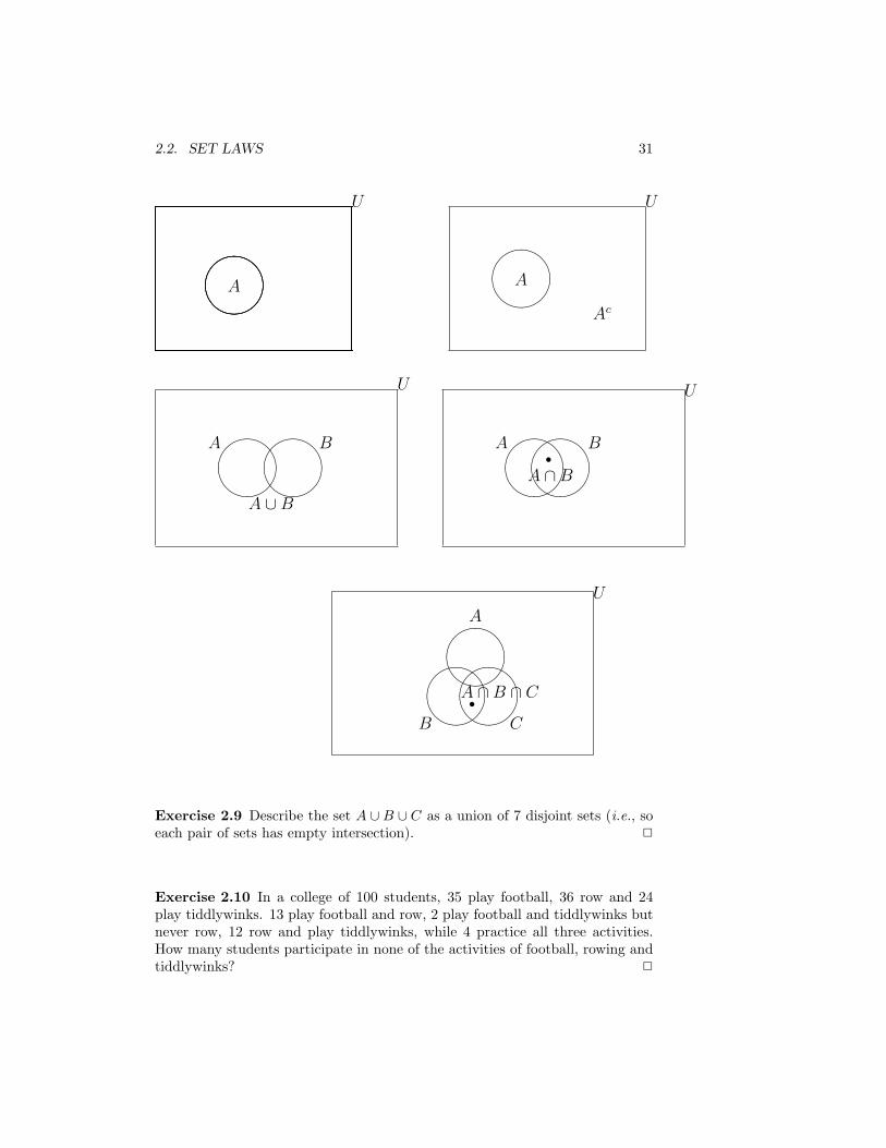
2.2.2 Venn diagrams
When an expression describing a set is small it can be viewed pictorially as aVenn diagram1 in which sets are represented as regions in the plane. In eachdiagram below the outer rectangle represents the universe U and the circles thesets A,B,C.
1After John Venn (1834-1923).
2.2. SET LAWS 31
&%'$&%'$&%'$
&%'$&%'$
&%'$&%'$
&%'$
&%'$&%'$
&%'$
A
U
U
A B
A ∪B
A
B C
A ∩B ∩ C•
U
Ac
A
A B•
A ∩B
U
U
Exercise 2.9 Describe the set A ∪B ∪ C as a union of 7 disjoint sets (i.e., soeach pair of sets has empty intersection). 2
Exercise 2.10 In a college of 100 students, 35 play football, 36 row and 24play tiddlywinks. 13 play football and row, 2 play football and tiddlywinks butnever row, 12 row and play tiddlywinks, while 4 practice all three activities.How many students participate in none of the activities of football, rowing andtiddlywinks? 2
32 CHAPTER 2. SETS AND LOGIC
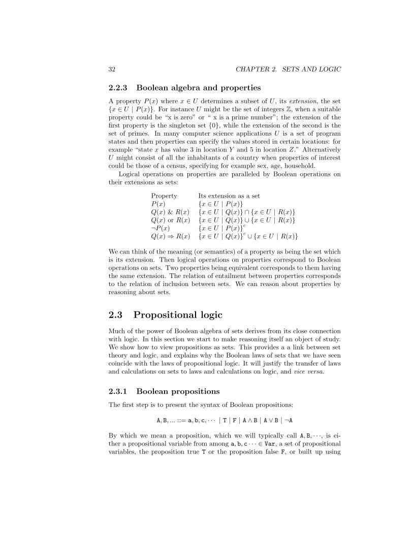
2.2.3 Boolean algebra and properties
A property P (x) where x ∈ U determines a subset of U , its extension, the set{x ∈ U | P (x)}. For instance U might be the set of integers Z, when a suitableproperty could be “x is zero” or “ x is a prime number”; the extension of thefirst property is the singleton set {0}, while the extension of the second is theset of primes. In many computer science applications U is a set of programstates and then properties can specify the values stored in certain locations: forexample “state x has value 3 in location Y and 5 in location Z.” AlternativelyU might consist of all the inhabitants of a country when properties of interestcould be those of a census, specifying for example sex, age, household.
Logical operations on properties are paralleled by Boolean operations ontheir extensions as sets:
Property Its extension as a setP (x) {x ∈ U | P (x)}Q(x) & R(x) {x ∈ U | Q(x)} ∩ {x ∈ U | R(x)}Q(x) or R(x) {x ∈ U | Q(x)} ∪ {x ∈ U | R(x)}¬P (x) {x ∈ U | P (x)}cQ(x)⇒ R(x) {x ∈ U | Q(x)}c ∪ {x ∈ U | R(x)}
We can think of the meaning (or semantics) of a property as being the set whichis its extension. Then logical operations on properties correspond to Booleanoperations on sets. Two properties being equivalent corresponds to them havingthe same extension. The relation of entailment between properties correspondsto the relation of inclusion between sets. We can reason about properties byreasoning about sets.
2.3 Propositional logic
Much of the power of Boolean algebra of sets derives from its close connectionwith logic. In this section we start to make reasoning itself an object of study.We show how to view propositions as sets. This provides a a link between settheory and logic, and explains why the Boolean laws of sets that we have seencoincide with the laws of propositional logic. It will justify the transfer of lawsand calculations on sets to laws and calculations on logic, and vice versa.
2.3.1 Boolean propositions
The first step is to present the syntax of Boolean propositions:
A, B, ... ::= a, b, c, · · · | T | F | A ∧ B | A ∨ B | ¬A
By which we mean a proposition, which we will typically call A, B, · · ·, is ei-ther a propositional variable from among a, b, c · · · ∈ Var, a set of propositionalvariables, the proposition true T or the proposition false F, or built up using
2.3. PROPOSITIONAL LOGIC 33
the logical operations of conjunction ∧, disjunction ∨ or negation ¬. We de-fine implication A ⇒ B to stand for ¬A ∨ B, and logical equivalence A ⇔ B as(A⇒ B) ∧ (B⇒ A). To avoid excessive brackets in writing Boolean propositionswe adopt the usual convention that the operation ¬ binds more tightly than thetwo other operations ∧ and ∨, so that ¬A ∨ B means (¬A) ∨ B.
Boolean propositions are ubiquitous in science and everyday life. They arean unavoidable ingredient of almost all precise discourse, and of course of math-ematics and computer science. They most often stand for simple assertionswe might make about the world, once we have fixed the meaning of the basicpropositional variables. For example, we might take the propositional variablesto mean basic propositions such as
“It’s raining”, “It’s sunny”, “Dave wears sunglasses”,“Lucy carries an umbrella”, . . .
which would allow us to describe more complex situations with Boolean propo-sitions, such as
“It’s sunny ∧ Dave wears sunglasses ∧ ¬(Lucy carries an umbrella)”.
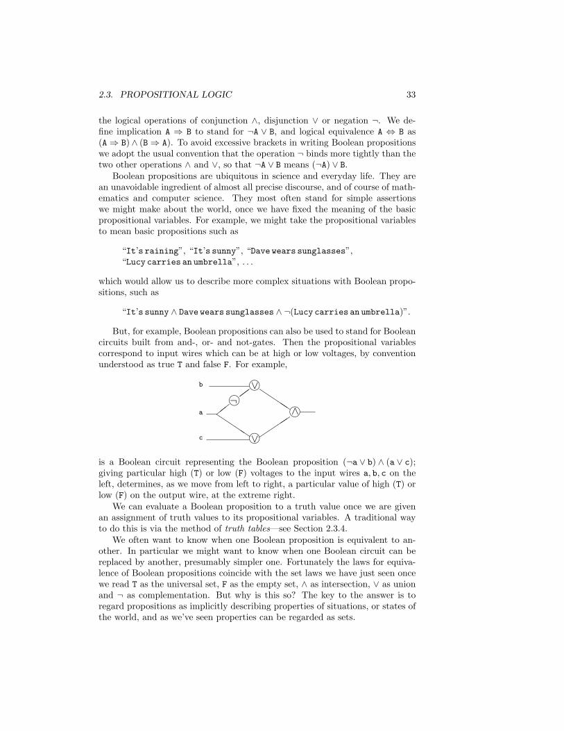
But, for example, Boolean propositions can also be used to stand for Booleancircuits built from and-, or- and not-gates. Then the propositional variablescorrespond to input wires which can be at high or low voltages, by conventionunderstood as true T and false F. For example,j
jjj Q
QQQ
����
##
��
QQQQ
b
a
c
∨¬
∨
∧
is a Boolean circuit representing the Boolean proposition (¬a ∨ b) ∧ (a ∨ c);giving particular high (T) or low (F) voltages to the input wires a, b, c on theleft, determines, as we move from left to right, a particular value of high (T) orlow (F) on the output wire, at the extreme right.
We can evaluate a Boolean proposition to a truth value once we are givenan assignment of truth values to its propositional variables. A traditional wayto do this is via the method of truth tables—see Section 2.3.4.
We often want to know when one Boolean proposition is equivalent to an-other. In particular we might want to know when one Boolean circuit can bereplaced by another, presumably simpler one. Fortunately the laws for equiva-lence of Boolean propositions coincide with the set laws we have just seen oncewe read T as the universal set, F as the empty set, ∧ as intersection, ∨ as unionand ¬ as complementation. But why is this so? The key to the answer is toregard propositions as implicitly describing properties of situations, or states ofthe world, and as we’ve seen properties can be regarded as sets.
34 CHAPTER 2. SETS AND LOGIC
2.3.2 Models
To link the set laws with logic, we show how to interpret Boolean propositionsas sets. The idea is to think of a proposition as denoting the set of states, orsituations, or worlds, or individuals, of which the proposition is true. The statesmight literally be states in a computer, but the range of propositional logic ismuch more general and it applies to any collection of situations, individuals orthings of which the properties of interest are either true or false. For this reasonwe allow interpretations to be very general, as formalised through the notion ofmodel.
A model M for Boolean propositions consists of a set UM, of states, calledthe universe of M, together with an interpretation [[A]]M of propositions A assubsets of UM which satisfies
[[T]]M = UM
[[F]]M = ∅[[A ∧ B]]M = [[A]]M ∩ [[B]]M[[A ∨ B]]M = [[A]]M ∪ [[B]]M
[[¬A]]M = [[A]]Mc.
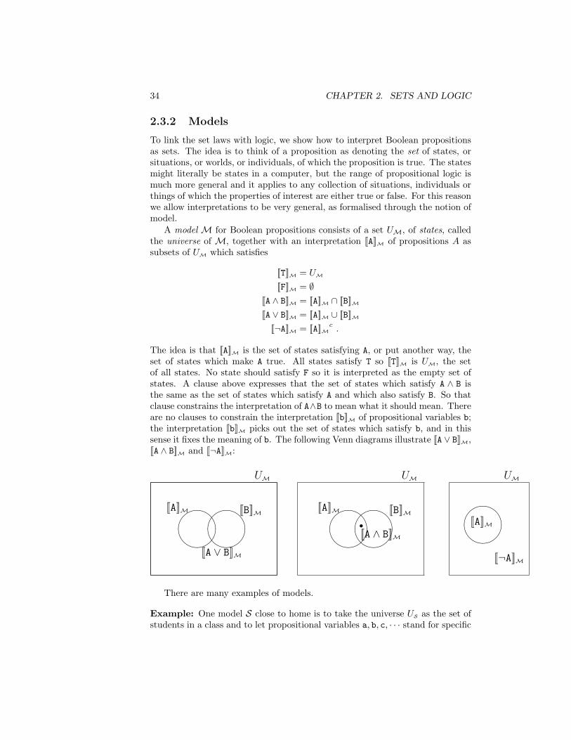
The idea is that [[A]]M is the set of states satisfying A, or put another way, theset of states which make A true. All states satisfy T so [[T]]M is UM, the setof all states. No state should satisfy F so it is interpreted as the empty set ofstates. A clause above expresses that the set of states which satisfy A ∧ B isthe same as the set of states which satisfy A and which also satisfy B. So thatclause constrains the interpretation of A∧B to mean what it should mean. Thereare no clauses to constrain the interpretation [[b]]M of propositional variables b;the interpretation [[b]]M picks out the set of states which satisfy b, and in thissense it fixes the meaning of b. The following Venn diagrams illustrate [[A ∨ B]]M,[[A ∧ B]]M and [[¬A]]M:
&%'$&%'$
&%'$&%'$
&%'$[[A]]M [[B]]M
[[A ∨ B]]M
UM
[[A]]M [[B]]M•[[A ∧ B]]M
[[A]]M
[[¬A]]M
UM UM
There are many examples of models.
Example: One model S close to home is to take the universe US as the set ofstudents in a class and to let propositional variables a, b, c, · · · stand for specific
2.3. PROPOSITIONAL LOGIC 35
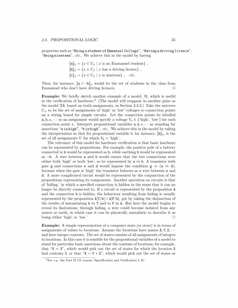
properties such as “Being a student of Emmanuel College”, “Having a driving licence”,“Being nineteen”, etc.. We achieve this in the model by having
[[a]]S = {x ∈ US | x is an Emmanuel student} ,[[b]]S = {x ∈ US | x has a driving licence} ,[[c]]S = {x ∈ US | x is nineteen} , etc.
Then, for instance, [[a ∧ ¬b]]S would be the set of students in the class fromEmmanuel who don’t have driving licences. 2
Example: We briefly sketch another example of a model, H, which is usefulin the verification of hardware.2 (The model will reappear in another guise asthe model TA, based on truth assignments, in Section 2.3.3.) Take the universeUH to be the set of assignments of ‘high’ or ‘low’ voltages to connection pointson a wiring board for simple circuits. Let the connection points be labelleda, b, c, · · · so an assignment would specify a voltage Vc ∈ {‘high’, ‘low’} for eachconnection point c. Interpret propositional variables a, b, c · · · as standing forassertions “a is high′′, “b is high”, etc.. We achieve this in the model by takingthe interpretation so that for propositional variable b, for instance, [[b]]H is theset of all assignments V for which Vb = ‘high’.
The relevance of this model for hardware verification is that basic hardwarecan be represented by propositions. For example, the positive pole of a batteryconnected to b would be represented as b, while earthing b would be representedas ¬b. A wire between a and b would ensure that the two connections wereeither both ‘high’ or both ‘low’, so be represented by a⇔ b. A transistor withgate g and connections s and d would impose the condition g ⇒ (s ⇔ d),because when the gate is ‘high’ the transistor behaves as a wire between s andd. A more complicated circuit would be represented by the conjunction of thepropositions representing its components. Another operation on circuits is thatof ‘hiding,’ in which a specified connection is hidden in the sense that it can nolonger be directly connected to. If a circuit is represented by the proposition Aand the connection b is hidden, the behaviour resulting from hiding is usuallyrepresented by the proposition A[T/b] ∨ A[F/b], got by taking the disjunction ofthe results of instantiating b to T and to F in A. But here the model begins toreveal its limitations; through hiding, a wire could become isolated from anysource or earth, in which case it can be physically unrealistic to describe it asbeing either ‘high’ or ‘low.’ 2
Example: A simple representation of a computer state (or store) is in terms ofassignments of values to locations. Assume the locations have names X, Y, Z, · · ·and have integer contents. The set of states consists of all assignments of integersto locations. In this case it is sensible for the propositional variables of a model tostand for particular basic assertions about the contents of locations; for example,that “X = 3”, which would pick out the set of states for which the location Xhad contents 3, or that “X = Y + Z”, which would pick out the set of states at
2See e.g. the Part II CS courses ‘Specification and Verification I, II.’
36 CHAPTER 2. SETS AND LOGIC
which the contents of location X equalled the contents of Y plus the contentsof Z. (The business of program verification often amounts to showing that if aprogram starts in state satisfying a particular proposition A, then after successfulexecution it ends in a state satisfying another particular proposition B.) 2
Validity and entailment
Using models we can make precise when a proposition is valid (i.e., always true)and when one proposition entails or is equivalent to another.
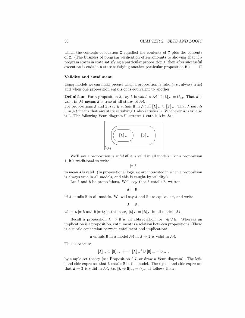
Definition: For a proposition A, say A is valid in M iff [[A]]M = UM. That A isvalid in M means A is true at all states of M.For propositions A and B, say A entails B in M iff [[A]]M ⊆ [[B]]M. That A entailsB inM means that any state satisfying A also satisfies B. Whenever A is true sois B. The following Venn diagram illustrates A entails B in M:
UM
'&
$%
����[[A]]M [[B]]M
We’ll say a proposition is valid iff it is valid in all models. For a propositionA, it’s traditional to write
|= A
to mean A is valid. (In propositional logic we are interested in when a propositionis always true in all models, and this is caught by validity.)
Let A and B be propositions. We’ll say that A entails B, written
A |= B ,
iff A entails B in all models. We will say A and B are equivalent, and write
A = B ,
when A |= B and B |= A; in this case, [[A]]M = [[B]]M in all models M.
Recall a proposition A ⇒ B is an abbreviation for ¬A ∨ B. Whereas animplication is a proposition, entailment is a relation between propositions. Thereis a subtle connection between entailment and implication:
A entails B in a model M iff A⇒ B is valid in M.
This is because
[[A]]M ⊆ [[B]]M ⇐⇒ [[A]]Mc ∪ [[B]]M = UM ,
by simple set theory (see Proposition 2.7, or draw a Venn diagram). The left-hand-side expresses that A entails B in the model. The right-hand-side expressesthat A⇒ B is valid in M, i.e. [[A⇒ B]]M = UM. It follows that:
2.3. PROPOSITIONAL LOGIC 37
Proposition 2.11 For Boolean propositions A, B,
A |= B iff |= (A⇒ B) .
An analogous result holds for equivalence:
Corollary 2.12 For Boolean propositions A, B,
A = B iff |= (A⇔ B) .
Proof.
A = B iff A |= B and B |= A
iff |= (A⇒ B) and |= (B⇒ A),by Proposition 2.11,iff |= (A⇒ B) ∧ (B⇒ A) (Why?), i.e. |= (A⇔ B) .
To answer ‘Why?’ above, notice that generally, for propositions C and D,
(|= C and |= D) iff [[C]]M = UM and [[D]]M = UM , for all models M,
iff [[C ∧ D]]M = UM , for all models M,
iff |= C ∧D .
2
2.3.3 Truth assignments
It’s probably not hard to convince yourself that whether a state in a modelsatisfies a proposition is determined solely by whether the propositional variablesare true or false there (and in fact we’ll prove this soon). This suggests a modelbased on states consisting purely of truth assignments, and leads us to reviewthe method of truth tables.
It is intended that a truth assignment should associate a unique truth valueT (for true) and F (for false) to each propositional variable a, b, c, · · · ∈ Var. Sowe define a truth assignment to be a set of propositional variables tagged bytheir associated truth values. An example of a truth assignment is the set
{aT, bF, cT, · · ·} ,
where we tag a by T to show it is assigned true and b by F to show that itis assigned false—we cannot have e.g. both aT and aF in the truth assignmentbecause the truth value assigned to a propositional variable has to be unique.3
3Later you’ll see that in effect a truth assignment is a set-theoretic function from Var tothe set {T, F}, but we don’t have that technology to hand just yet.
38 CHAPTER 2. SETS AND LOGIC
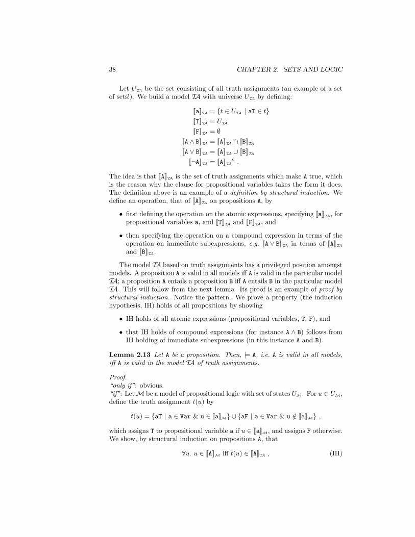
Let UTA be the set consisting of all truth assignments (an example of a setof sets!). We build a model TA with universe UTA by defining:
[[a]]TA = {t ∈ UTA | aT ∈ t}[[T]]TA = UTA
[[F]]TA = ∅[[A ∧ B]]TA = [[A]]TA ∩ [[B]]TA[[A ∨ B]]TA = [[A]]TA ∪ [[B]]TA
[[¬A]]TA = [[A]]TAc.
The idea is that [[A]]TA is the set of truth assignments which make A true, whichis the reason why the clause for propositional variables takes the form it does.The definition above is an example of a definition by structural induction. Wedefine an operation, that of [[A]]TA on propositions A, by
• first defining the operation on the atomic expressions, specifying [[a]]TA, forpropositional variables a, and [[T]]TA and [[F]]TA, and
• then specifying the operation on a compound expression in terms of theoperation on immediate subexpressions, e.g. [[A ∨ B]]TA in terms of [[A]]TAand [[B]]TA.
The model TA based on truth assignments has a privileged position amongstmodels. A proposition A is valid in all models iff A is valid in the particular modelTA; a proposition A entails a proposition B iff A entails B in the particular modelTA. This will follow from the next lemma. Its proof is an example of proof bystructural induction. Notice the pattern. We prove a property (the inductionhypothesis, IH) holds of all propositions by showing
• IH holds of all atomic expressions (propositional variables, T, F), and
• that IH holds of compound expressions (for instance A ∧ B) follows fromIH holding of immediate subexpressions (in this instance A and B).
Lemma 2.13 Let A be a proposition. Then, |= A, i.e. A is valid in all models,iff A is valid in the model TA of truth assignments.
Proof.“only if”: obvious.“if”: LetM be a model of propositional logic with set of states UM. For u ∈ UM,define the truth assignment t(u) by
t(u) = {aT | a ∈ Var & u ∈ [[a]]M} ∪ {aF | a ∈ Var & u /∈ [[a]]M} ,
which assigns T to propositional variable a if u ∈ [[a]]M, and assigns F otherwise.We show, by structural induction on propositions A, that
∀u. u ∈ [[A]]M iff t(u) ∈ [[A]]TA , (IH)
2.3. PROPOSITIONAL LOGIC 39
for all propositions A. (The statement IH is the induction hypothesis.) Theproof splits into cases according to the syntactic form of A. (We use ≡ for therelation of syntactic identity.)
A ≡ a, a propositional variable. By the definition of t(u),
u ∈ [[a]]M ⇐⇒ aT ∈ t(u)⇐⇒ t(u) ∈ [[a]]TA .
Hence the induction hypothesis IH holds for propositional variables.
A ≡ T: In this case IH holds because both u ∈ [[T]]M and t(u) ∈ [[T]]TA for allu ∈ UM.
A ≡ F: In this case IH holds because both u 6∈ [[T]]M and t(u) 6∈ [[T]]TA for allu ∈ UM.
A ≡ B ∧ C. In this case the task is to show that IH holds for B and for C impliesIH holds for B ∧ C. Assume that IH holds for B and C. Then,
u ∈ [[B ∧ C]]M ⇐⇒ u ∈ [[B]]M and u ∈ [[C]]M, as M is a model,⇐⇒ t(u) ∈ [[B]]TA and t(u) ∈ [[C]]TA, by the induction hypothesis,⇐⇒ t(u) ∈ [[B ∧ C]]TA, as TA is a model.
A ≡ B ∨ C. Similarly we argue
u ∈ [[B ∨ C]]M ⇐⇒ u ∈ [[B]]M or u ∈ [[C]]M, as M is a model,⇐⇒ t(u) ∈ [[B]]TA or t(u) ∈ [[C]]TA, by the induction hypothesis,⇐⇒ t(u) ∈ [[B ∨ C]]TA, as TA is a model.
A ≡ ¬B. We argue
u ∈ [[¬B]]M ⇐⇒ u /∈ [[B]]M, as M is a model,⇐⇒ t(u) /∈ [[B]]TA, by the induction hypothesis.
By structural induction we conclude that the induction hypothesis holdsfor all propositions A. We deduce that if [[A]]TA = UTA, the set of all truthassignments, then [[A]]M = UM for any model M, and hence A is valid. 2
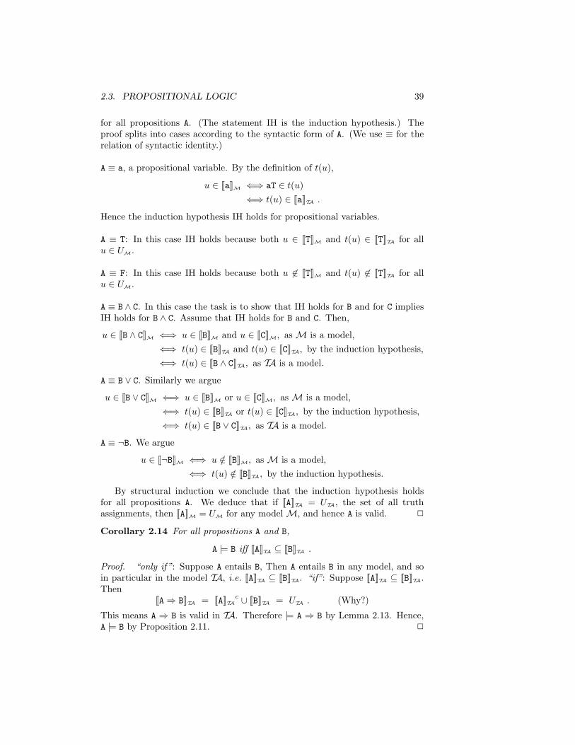
Corollary 2.14 For all propositions A and B,
A |= B iff [[A]]TA ⊆ [[B]]TA .
Proof. “only if”: Suppose A entails B, Then A entails B in any model, and soin particular in the model TA, i.e. [[A]]TA ⊆ [[B]]TA. “if”: Suppose [[A]]TA ⊆ [[B]]TA.Then
[[A⇒ B]]TA = [[A]]TAc ∪ [[B]]TA = UTA . (Why?)
This means A ⇒ B is valid in TA. Therefore |= A ⇒ B by Lemma 2.13. Hence,A |= B by Proposition 2.11. 2
40 CHAPTER 2. SETS AND LOGIC
2.3.4 Truth tables
Lemma 2.13 explains the widespread applicability of a calculational methodthat you already know. A way to check a proposition is valid, so true in anyconceivable model in any conceivable state, is via the well-known method oftruth tables.
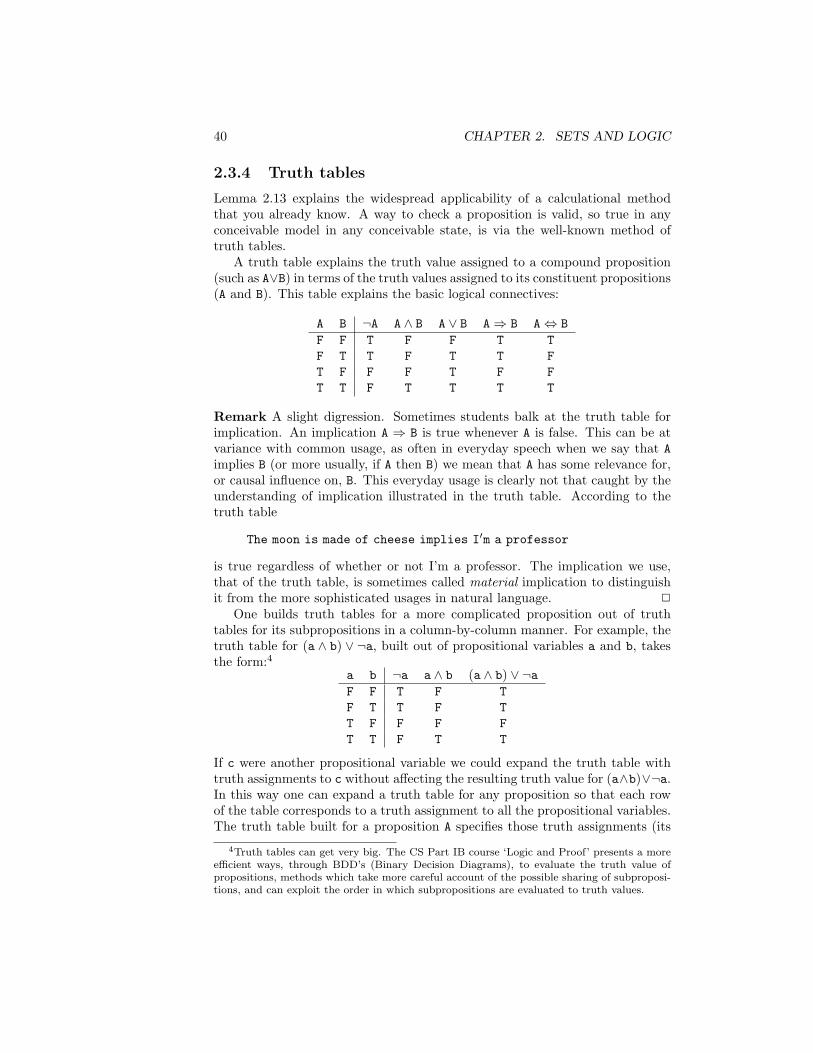
A truth table explains the truth value assigned to a compound proposition(such as A∨B) in terms of the truth values assigned to its constituent propositions(A and B). This table explains the basic logical connectives:
A B ¬A A ∧ B A ∨ B A⇒ B A⇔ BF F T F F T TF T T F T T FT F F F T F FT T F T T T T
Remark A slight digression. Sometimes students balk at the truth table forimplication. An implication A ⇒ B is true whenever A is false. This can be atvariance with common usage, as often in everyday speech when we say that Aimplies B (or more usually, if A then B) we mean that A has some relevance for,or causal influence on, B. This everyday usage is clearly not that caught by theunderstanding of implication illustrated in the truth table. According to thetruth table
The moon is made of cheese implies I′m a professor
is true regardless of whether or not I’m a professor. The implication we use,that of the truth table, is sometimes called material implication to distinguishit from the more sophisticated usages in natural language. 2
One builds truth tables for a more complicated proposition out of truthtables for its subpropositions in a column-by-column manner. For example, thetruth table for (a ∧ b) ∨ ¬a, built out of propositional variables a and b, takesthe form:4
a b ¬a a ∧ b (a ∧ b) ∨ ¬aF F T F TF T T F TT F F F FT T F T T
If c were another propositional variable we could expand the truth table withtruth assignments to c without affecting the resulting truth value for (a∧b)∨¬a.In this way one can expand a truth table for any proposition so that each rowof the table corresponds to a truth assignment to all the propositional variables.The truth table built for a proposition A specifies those truth assignments (its
4Truth tables can get very big. The CS Part IB course ‘Logic and Proof’ presents a moreefficient ways, through BDD’s (Binary Decision Diagrams), to evaluate the truth value ofpropositions, methods which take more careful account of the possible sharing of subproposi-tions, and can exploit the order in which subpropositions are evaluated to truth values.
2.3. PROPOSITIONAL LOGIC 41
rows) that result in the proposition A being true. This is just another way todescribe [[A]]TA, the set of truth assignments that make A true. The propositionA is valid iff it is true for all truth assignments. We see this in its truth tablethrough A being assigned T in every row. Such a proposition is traditionallycalled a tautology.
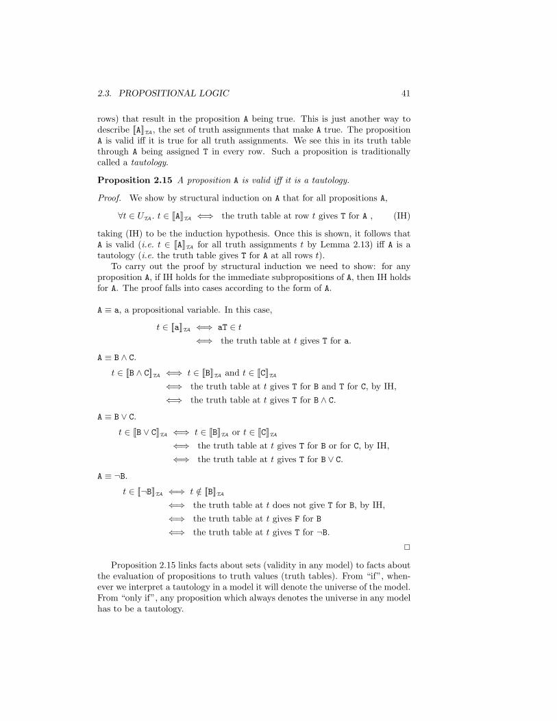
Proposition 2.15 A proposition A is valid iff it is a tautology.
Proof. We show by structural induction on A that for all propositions A,
∀t ∈ UTA. t ∈ [[A]]TA ⇐⇒ the truth table at row t gives T for A , (IH)
taking (IH) to be the induction hypothesis. Once this is shown, it follows thatA is valid (i.e. t ∈ [[A]]TA for all truth assignments t by Lemma 2.13) iff A is atautology (i.e. the truth table gives T for A at all rows t).
To carry out the proof by structural induction we need to show: for anyproposition A, if IH holds for the immediate subpropositions of A, then IH holdsfor A. The proof falls into cases according to the form of A.
A ≡ a, a propositional variable. In this case,
t ∈ [[a]]TA ⇐⇒ aT ∈ t⇐⇒ the truth table at t gives T for a.
A ≡ B ∧ C.
t ∈ [[B ∧ C]]TA ⇐⇒ t ∈ [[B]]TA and t ∈ [[C]]TA⇐⇒ the truth table at t gives T for B and T for C, by IH,⇐⇒ the truth table at t gives T for B ∧ C.
A ≡ B ∨ C.
t ∈ [[B ∨ C]]TA ⇐⇒ t ∈ [[B]]TA or t ∈ [[C]]TA⇐⇒ the truth table at t gives T for B or for C, by IH,⇐⇒ the truth table at t gives T for B ∨ C.
A ≡ ¬B.
t ∈ [[¬B]]TA ⇐⇒ t /∈ [[B]]TA⇐⇒ the truth table at t does not give T for B, by IH,⇐⇒ the truth table at t gives F for B⇐⇒ the truth table at t gives T for ¬B.
2
Proposition 2.15 links facts about sets (validity in any model) to facts aboutthe evaluation of propositions to truth values (truth tables). From “if”, when-ever we interpret a tautology in a model it will denote the universe of the model.From “only if”, any proposition which always denotes the universe in any modelhas to be a tautology.
42 CHAPTER 2. SETS AND LOGIC
2.3.5 Methods
We can use truth tables to show an entailment A |= B, or an equivalence A = B.Recall Proposition 2.11, that
A |= B iff |= A⇒ B .
So, by Proposition 2.15, one way to show A |= B is to show that (A ⇒ B) is atautology. But this amounts to showing that in any row (so truth assignment)where A gives T so does B—B may give T on more rows than A. Conversely, ifA |= B, then any truth assignment making A true will make B true—a fact whichtransfers to their truth tables. For example, you can easily check that the truthtables for A ∨ B and ¬(¬A ∧ ¬B) are the same; hence A ∨ B = ¬(¬A ∧ ¬B). (Infact, we could have been even more parsimonious in the syntax of propositions,and taken A ∨ B to be an abbreviation for ¬(¬A ∧ ¬B).)
Truth tables are one way to establish the equivalence A = B of propositionsA and B: check that the truth tables for A and B yield the same truth valueson corresponding rows. But propositions stand for sets in any model so we canalso use the identities of Boolean algebra to simplify propositions, treating con-junctions as intersections, disjunctions as unions and negations as complements.For example, from the De Morgan and Complement laws
¬(a ∧ ¬b) = ¬a ∨ ¬¬b= ¬a ∨ b .
As here we can make use of the fact that equivalence is substitutive in thefollowing sense. Once we know two propositions B and B′ are equivalent, if wehave another proposition C in which B occurs we can replace some or all of itsoccurrences by B′ and obtain an equivalent proposition C′. One way to see thisis by considering the truth table of C—the eventual truth value obtained will beunaffected if B′ stands in place of B, provided B = B′. This means that we canhandle equivalence just as the equality of school algebra. (Exercise 2.25 guidesyou through a proof of the property of substitutivity of equivalence.)
Generally, using the set identities any proposition can be transformed todisjunctive form as a disjunction of conjunctions of propositional variables andtheir negations, or alternatively to conjunctive form as a conjunction of disjunc-tions of propositional variables and their negations, e.g.:
· · · ∨ (¬a1 ∧ a2 ∧ · · · ∧ ak) ∨ · · ·· · · ∧ (¬a1 ∨ a2 ∨ · · · ∨ ak) ∧ · · ·
With the help of the Idempotence and Complement laws we can remove redun-dant occurrences of propositional variables to obtain normal forms (unique upto reordering), respectively disjunctive and conjunctive normal forms for propo-sitions. The equivalence of two propositions can be checked by comparing theirnormal forms. The normal forms play a central role in theorem proving.
Exercise 2.16 Using the set laws express ¬(a∨b)∨(a∧c) in conjunctive form.2
2.3. PROPOSITIONAL LOGIC 43
Exercise 2.17 Do this exercise without using Proposition 2.15.(i) Using the method of truth tables show (¬B⇒ ¬A) = (A⇒ B). Deduce
(¬B⇒ ¬A)⇔ (A⇒ B)
is a tautology.(ii) Show in any model M that
[[¬B⇒ ¬A]]M = [[A⇒ B]]M ;
deduce|= [(¬B⇒ ¬A)⇔ (A⇒ B)] .
Parts (i) and (ii) give two methods for demonstrating entailments and tau-tologies linked by Proposition 2.15 . Method (ii) might look long-winded. How-ever in practice one can drop the [[−]]M brackets, think of propositions as setsand use Venn diagrams or the set identities to simplify set expressions (just aswe did above in simplifying ¬(a ∧ ¬b)). 2
Exercise 2.18
(i) Show that A⇔ B = (A ∧ B) ∨ (¬A ∧ ¬B).
(ii) Show that A⇔ (B ⇔ C) = (A⇔ B)⇔ C.[The analogous result does not hold when⇔ is replaced by⇒—why not?]
(iii) Show that ¬(B ⇔ C) = ((¬B)⇔ C).
2
Exercise 2.19 Sheffer’s stroke is not an affliction but a logical operation A|Bout of which all the usual logical operations can be derived. It is defined by thefollowing truth table:
A B A|BF F TF T TT F TT T F
Check that A|B = ¬(A ∧ B) by showing that they have the same truth table.Describe how to define the operations of negation, conjunction and disjunctionout of Sheffer’s stroke. 2
Exercise 2.20 Verify that Peirce’s law, ((A⇒ B)⇒ A)⇒ A, is a tautology. 2
Exercise 2.21 Simplify the Boolean proposition
¬(¬(a ∧ ¬(a ∧ b)) ∧ ¬(¬(a ∧ b) ∧ b)) .
2
44 CHAPTER 2. SETS AND LOGIC
Exercise 2.22 Simplify [(a ⇒ b) ∨ (a ⇒ d)] ⇒ (b ∨ d) to the propositiona ∨ b ∨ d. 2
Exercise 2.23 Consider the argument: “If Anna can cancan or Kant can’tcant, then Greville will cavil vilely. If Greville will cavil vilely, Will will want.But Will won’t want. Therefore Kant can cant.” By writing the statement inquotes as a proposition in terms of four propositional variables and simplifying,show that it is a tautology and hence that the argument holds. 2
Exercise 2.24 Define the length of a Boolean proposition by structural induc-tion as follows:
|a| = 1, |T| = 1, |F| = 1,|A ∧ B| = |A|+ |B|+ 1,|A ∨ B| = |A|+ |B|+ 1, |¬A| = |A|+ 1 .
Define a translation which eliminates disjunction from Boolean expressions bythe following structural induction:
tr(a) = a, tr(T) = T, tr(F) = F,
tr(A ∧ B) = tr(A) ∧ tr(B),tr(A ∨ B) = ¬(¬tr(A) ∧ ¬tr(B)), tr(¬A) = ¬tr(A) .
Prove by structural induction on Boolean propositions that
|tr(A)| ≤ 3|A| − 1 ,
for all Boolean propositions A. 2
Exercise 2.25 Define a Boolean propositional context to be given by
C, C′, ... ::= a, b, c, · · · | T | F | [ ] | C ∧ C′ | C ∨ C′ | ¬C
where a, b, c · · · ∈ Var. So a context is like a Boolean proposition but possiblywith several occurrences of a ‘hole’ [ ], into which a Boolean proposition can besubstituted. Define the substitution C[B] of a proposition B into a context C bystructural induction on contexts as follows:
a[B] = a, T[B] = T, F[B] = F, [ ][B] = B,
(C ∧ C′)[B] = C[B] ∧ C′[B], (C ∨ C′)[B] = C[B] ∨ C′[B],¬C[B] = ¬(C[B]) .
Prove by structural induction on contexts that, for all contexts C,
if B and B′ are propositions for which B = B′, then C[B] = C[B′].
2
Chapter 3
Relations and functions
In this chapter we study how to relate, possibly different, sets through the set-theoretic definitions of relation and function. We will rely on the product of setsas the central construction for connecting sets. We are led to consider sets withextra structure, and the cardinality of sets, in particular the important notionof countability.
3.1 Ordered pairs and products
Given two elements a, b we can form their ordered pair (a, b). Two ordered pairsare equal iff their first components are equal and their second components areequal too, i.e.
(a, b) = (a′, b′) ⇐⇒ a = a′ & b = b′ .
There is also the concept of unordered pair of elements a, b—this is just the set{a, b}. We’ll only rarely use unordered pairs so “pair” alone will mean orderedpair.
Often you’ll see the ordered pair (a, b) defined to be the set {{a}, {a, b}}—this is one particular way of coding the idea of ordered pair as a set. (SeeExercise 3.2 below. Apart from this exercise we’ll never again consider howordered pairs are implemented.)
For sets X and Y , their product is the set
X × Y = {(a, b) | a ∈ X & b ∈ Y },
the set of all ordered pairs of elements with the first from X and the secondfrom Y .
We can use the product construction on sets several times. A ternary productof sets X×Y ×Z, consisting of triples (x, y, z), can be understood as X×(Y ×Z),and so on. In the case where all the sets in a product are the same, as in X×Xwe often write the product as X2, with X×X×X written as X3, and generallya product X × · · · × X, the product of n copies of X, as Xn. Such products
45
46 CHAPTER 3. RELATIONS AND FUNCTIONS
are familiar from coordinate geometry: a point on a line can be identified witha real number in R, the set of real numbers; the points on the plane can beidentified with elements of the product R × R, which we can also write as R2;three-dimensional space with R3, and so on.
Exercise 3.1 Prove
(i) A× (B ∪ C) = (A×B) ∪ (A× C)
(ii) A× (B ∩ C) = (A×B) ∩ (A× C)
(iii) (A×B) ∩ (C ×D) = (A ∩ C)× (B ∩D)
(iv) (A×B)∪ (C×D) ⊆ (A∪C)× (B ∪D) [Show the converse inclusion doesnot hold in general.]
2
Exercise 3.2 Show that a set {{a}, {a, b}} behaves as an ordered pair should,i.e.
{{a}, {a, b}} = {{a′}, {a′, b′}} ⇐⇒ a = a′ & b = b′ .
[This is trickier than you might at first think. Consider the two cases a = b anda 6= b.] 2
3.2 Relations and functions
A binary relation between X and Y is a subset R ⊆ X×Y—so a subset of pairsin the relation. We shall often write xRy for (x, y) ∈ R.
Let R ⊆ X × Y . Write R−1 for the converse, or inverse, relation R−1 ={(y, x) | (x, y) ∈ R}; so R−1 ⊆ Y ×X with yR−1x iff xRy.
A partial function from X to Y is a relation f ⊆ X × Y for which
∀x, y, y′. (x, y) ∈ f & (x, y′) ∈ f ⇒ y = y′.
We use the notation f(x) = y when there is a y such that (x, y) ∈ f and thensay f(x) is defined, and otherwise say f(x) is undefined; the set
{x ∈ X | f(x) is defined}
is called the domain of definition of the partial function f . Sometimes we writef : x 7→ y, or just x 7→ y when f is understood, for y = f(x). Occasionally onesees just fx, without the brackets, for f(x).
A (total) function from X to Y is a partial function from X to Y such thatfor all x ∈ X there is some y ∈ Y such that f(x) = y. Although total functionsare a special kind of partial function it is traditional to understand somethingdescribed as simply a function to be a total function, so we always say explicitlywhen a function is partial.
3.2. RELATIONS AND FUNCTIONS 47
To stress the fact that we are thinking of a function f from X to Y astaking an element of X and yielding an element of Y we generally write it asf : X → Y . To indicate a partial function f from X to Y we write f : X ⇀ Y .For both functions and partial functions from X to Y , the set X is called thedomain of the function and Y the codomain of the function.
Note that individual relations and functions are also sets. This fact deter-mines equality between relations, and equality between functions; they are equaliff they consist of the same set of pairs. We can reword this fact in the case offunctions and partial functions.
Proposition 3.3
(i) Let R,R′ ⊆ X × Y . Then,
R = R′ iff ∀x ∈ X, y ∈ Y. xRy ⇐⇒ xR′y .
(ii) Let f, f ′ : X → Y . Then,
f = f ′ iff ∀x ∈ X. f(x) = f ′(x) .
(iii) Let f, f ′ : X ⇀ Y . Then,
f = f ′ iff ∀x ∈ X. (f(x) is defined ⇒ f ′(x) is defined & f(x) = f ′(x)) &(f ′(x) is defined ⇒ f(x) is defined & f(x) = f ′(x)) .
So, to investigate whether two functions with the same domain and codomainare equal it suffices to show that they give the same results when applied to anarbitrary common argument.
Exercise 3.4 If A has k elements and B has m elements, how many relationsare there between A and B? 2
Exercise 3.5 Let R and S be relations between A and B. Show that, if R ⊆ S,then R−1 ⊆ S−1. Prove that (R∩S)−1 = R−1∩S−1 and (R∪S)−1 = R−1∪S−1.
2
Exercise 3.6 If A and B are finite sets with m and n elements respectively,how many functions and how many partial functions are there from A to B? 2
3.2.1 Composing relations and functions
We compose relations, and so partial and total functions, R between X and Yand S between Y and Z by defining their composition, a relation between Xand Z, by
S ◦R =def {(x, z) ∈ X × Z | ∃y ∈ Y. (x, y) ∈ R & (y, z) ∈ S} .
Let R ⊆ X × Y , S ⊆ Y ×Z and T ⊆ Z ×W . It should not be hard to convinceyourself that
T ◦ (S ◦R) = (T ◦ S) ◦Ri.e. composition is associative.
48 CHAPTER 3. RELATIONS AND FUNCTIONS
Exercise 3.7 Let A = {1, 2, 3, 4}, B = {a, b, c, d} and C = {x, y, z}. LetR = {(1, a), (2, d), (3, a), (3, b), (3, d)} and S = {(b, x), (b, z), (c, y), (d, z)}. Whatis their composition S ◦R? 2
Exercise 3.8 Show that the composition of relations is associative. 2
Each setX is associated with an identity relation idX where idX = {(x, x) | x ∈ X}.It is easy to see that for any relation R between X and Y
R ◦ idX = idY ◦R = R
—so the identity relation does indeed behave like an identity with respect tocomposition. Note that the identity relation is a function.
For functions f : X → Y and g : Y → Z their composition is also a functiong◦f : X → Z (check!). Similarly, the composition of partial functions f : X ⇀ Yand g : Y ⇀ Z is a partial function g ◦ f : X ⇀ Z (check!).
We say a function f : X → Y is injective (or 1-1) iff
∀x, x′ ∈ X. f(x) = f(x′)⇒ x = x′ .
In other words, taking the contrapositive of this implication, distinct elements ofX go to distinct elements of Y . An injective function is often called an injection.
We say a function f : X → Y is surjective (or onto) iff
∀y ∈ Y ∃x ∈ X. y = f(x) .
A surjective function is often called an surjection.A function f : X → Y is bijective iff it is both injective and surjective.
Bijective functions f : X → Y are called bijections; the sets X and Y are saidto be in 1-1 correspondence, or bijective correspondence.
A function f : X → Y has an inverse function g : Y → X iff g(f(x)) = x forall x ∈ X, and f(g(y)) = y for all y ∈ Y . Notice the symmetry: f has inverse gmeans g has inverse f , and vice versa.
Lemma 3.9 A function f : X → Y is bijective iff it has an inverse function.
Proof.‘if”: Suppose f : X → Y has an inverse g : Y → X. Let x, x′ ∈ X and supposef(x) = f(x′). Then
x = g(f(x)) = g(f(x′)) = x′ .
Hence f is injective. Let y ∈ Y . Then f(g(y)) = y. Hence f is surjective. Itfollows that f is bijective.“only if”: Assume f : X → Y is bijective. Define the relation g ⊆ Y × X byg = f−1, the converse relation of f , so (y, x) ∈ g ⇐⇒ f(x) = y.
Suppose (y, x), (y, x′) ∈ g. Then, f(x) = y and f(x′) = y, so x = x′ as fis injective. Given y ∈ Y there is x ∈ X such that f(x) = y as f is surjective,
3.2. RELATIONS AND FUNCTIONS 49
making (y, x) ∈ g. This shows that g is a function g : Y → X which moreoversatisfies
g(y) = x ⇐⇒ f(x) = y . (†)
We now deduce that g is injective. Suppose g(y) = g(y′), where y, y′ ∈ Y .Letting x = g(y) = g(y′) we see from (†) that both f(x) = y and f(x) = y′,whence y = y′.
If g(f(x)) = x′ then f(x′) = f(x) by (†), so x = x′, as f is injective. Iff(g(y)) = y′ then g(y′) = g(y) by (†), so y = y′, as g is injective. This showsthat g is an inverse to f . 2
Suppose f : X → Y has an inverse g : Y → X. Then g has f as its inverse.So by Lemma 3.9, both f and g are bijective. It is traditional to write f−1 forthe inverse of a function f .
Exercise 3.10 Show that the composition of injective/surjective/bijective func-tions is respectively injective/surjective/bijective. 2
Exercise 3.11 Let D be the set {x ∈ R | x > 1}. Define a binary relationg ⊆ D ×D by taking
(u, v) ∈ g iff1u
+1v
= 1 .
(i) Express v as a formula in u for (u, v) ∈ g. Deduce that g is a functiong : D → D.
(ii) Define f an inverse function to g and prove that it has the desired prop-erties, viz. thatf ◦ g = idD and g ◦ f = idD. Deduce that g : D → D is abijection.
[The formula 1u + 1
v = 1 expresses the relation between the distance of an objectu and the distance of its image v from a lens with focal length 1.] 2
3.2.2 Direct and inverse image under a relation
We extend relations, and thus partial and total functions, R ⊆ X × Y to anoperation acting on subsets by taking
R A = {y ∈ Y | ∃x ∈ A. (x, y) ∈ R}
for A ⊆ X. The set R A is called the direct image of A under R. We define
R−1B = {x ∈ X | ∃y ∈ B. (x, y) ∈ R}
for B ⊆ Y . The set R−1B is called the inverse image of B under R; note that itis the same set as the direct image of the set B under the converse, or inverse,relation R−1. Of course, the same notions of direct and inverse image also applyin the special cases where the relation is a partial function or function.
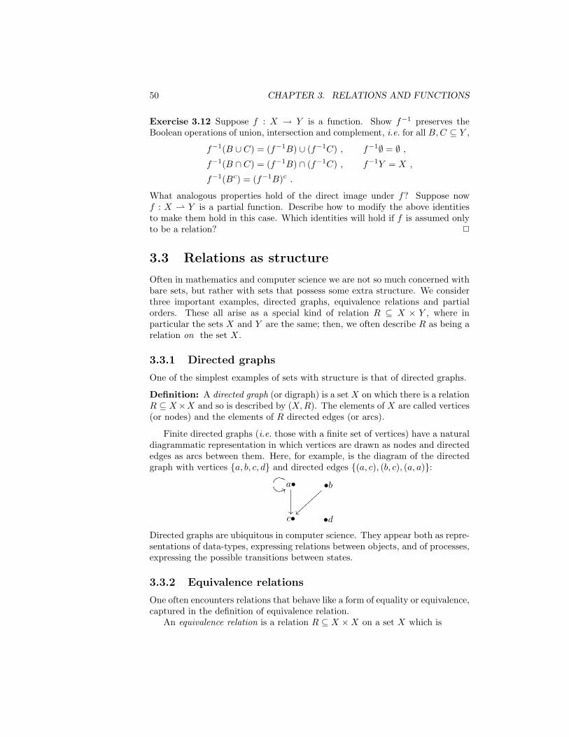
50 CHAPTER 3. RELATIONS AND FUNCTIONS
Exercise 3.12 Suppose f : X → Y is a function. Show f−1 preserves theBoolean operations of union, intersection and complement, i.e. for all B,C ⊆ Y ,
f−1(B ∪ C) = (f−1B) ∪ (f−1C) , f−1∅ = ∅ ,f−1(B ∩ C) = (f−1B) ∩ (f−1C) , f−1Y = X ,
f−1(Bc) = (f−1B)c .
What analogous properties hold of the direct image under f? Suppose nowf : X ⇀ Y is a partial function. Describe how to modify the above identitiesto make them hold in this case. Which identities will hold if f is assumed onlyto be a relation? 2
3.3 Relations as structure
Often in mathematics and computer science we are not so much concerned withbare sets, but rather with sets that possess some extra structure. We considerthree important examples, directed graphs, equivalence relations and partialorders. These all arise as a special kind of relation R ⊆ X × Y , where inparticular the sets X and Y are the same; then, we often describe R as being arelation on the set X.
3.3.1 Directed graphs
One of the simplest examples of sets with structure is that of directed graphs.
Definition: A directed graph (or digraph) is a set X on which there is a relationR ⊆ X×X and so is described by (X,R). The elements of X are called vertices(or nodes) and the elements of R directed edges (or arcs).
Finite directed graphs (i.e. those with a finite set of vertices) have a naturaldiagrammatic representation in which vertices are drawn as nodes and directededges as arcs between them. Here, for example, is the diagram of the directedgraph with vertices {a, b, c, d} and directed edges {(a, c), (b, c), (a, a)}:
a•88
��
•b
~~||||||||
c• •d
Directed graphs are ubiquitous in computer science. They appear both as repre-sentations of data-types, expressing relations between objects, and of processes,expressing the possible transitions between states.
3.3.2 Equivalence relations
One often encounters relations that behave like a form of equality or equivalence,captured in the definition of equivalence relation.
An equivalence relation is a relation R ⊆ X ×X on a set X which is
3.3. RELATIONS AS STRUCTURE 51
• reflexive: ∀x ∈ X. xRx,
• symmetric: ∀x, y ∈ X. xRy ⇒ yRx and
• transitive: ∀x, y, z ∈ X. xRy & yRz ⇒ xRz.
If R is an equivalence relation on X then the (R-)equivalence class of anelement x ∈ X is the subset {x}R =def {y ∈ X | yRx}.
An equivalence relation on a set X determines a partition of X. A partitionof a set X is a set P of non-empty subsets of X for which each element x of Xbelongs to one and only one member of P . In other words, a partition P of Xis a collection of nonempty, disjoint subsets of X such that each element x of Xbelongs to a member of P .
Theorem 3.13 Let R be an equivalence relation on a set X. The set X/R =def
{{x}R | x ∈ X} of equivalence classes with respect to R is a partition of the setX. Moreover, {x}R = {y}R iff xRy for all x, y ∈ X.
Proof. Let x ∈ X. Then as R is reflexive, x ∈ {x}R. So every member of X/Ris nonempty and each element of X belongs to a member of X/R. For X/R tobe a partition we also require that its members are disjoint. However, we willshow
(1) {x}R ∩ {y}R 6= ∅ ⇒ xRy , and(2) xRy ⇒ {x}R = {y}R ,
from which {x}R∩{y}R 6= ∅ ⇒ {x}R = {y}R follows, for any elements x, y ∈ X.
(1) Suppose {x}R ∩{y}R 6= ∅. Then there is some z ∈ {x}R ∩{y}R. Hence zRxand zRy. Then xRz and zRy, as R is symmetric. As R is transitive we obtainxRy.
(2) Suppose xRy. Let w ∈ {x}R. Then wRx and xRy, so wRy by transitivityof R. Thus w ∈ {y}R. This shows {x}R ⊆ {y}R. Because R is symmetric wehave yRx and so by a similar argument we also obtain {y}R ⊆ {x}R. Hence{x}R = {y}R.
If {x}R = {y}R, then certainly x ∈ {x}R ∩ {y}R, so xRy by (1). Combiningwith (2) we see that {x}R = {y}R iff xRy for all x, y ∈ X. 2
There is a simple converse to Theorem 3.13:
Proposition 3.14 Let P be a partition of a set X. The relation R on X,defined by
xRy ⇐⇒ ∃p ∈ P. x ∈ p & y ∈ p ,is an equivalence relation on the set X with X/R = P .
Exercise 3.15 Provide the proof to Proposition 3.14. 2
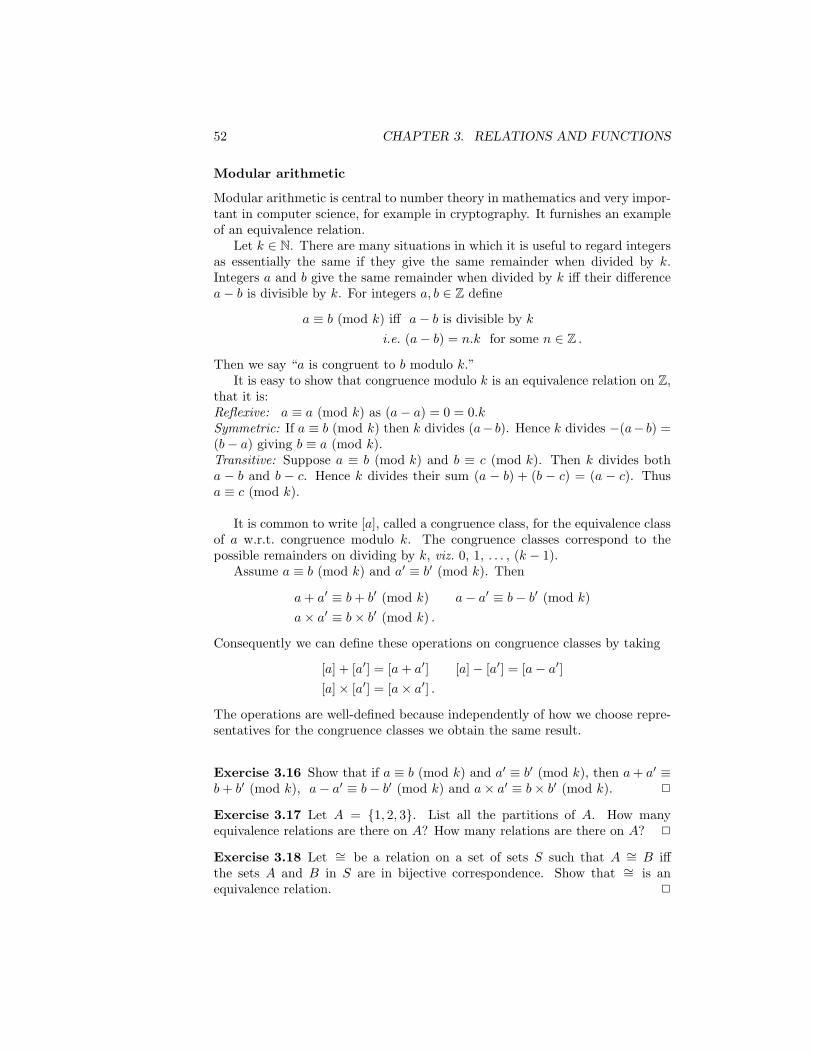
52 CHAPTER 3. RELATIONS AND FUNCTIONS
Modular arithmetic
Modular arithmetic is central to number theory in mathematics and very impor-tant in computer science, for example in cryptography. It furnishes an exampleof an equivalence relation.
Let k ∈ N. There are many situations in which it is useful to regard integersas essentially the same if they give the same remainder when divided by k.Integers a and b give the same remainder when divided by k iff their differencea− b is divisible by k. For integers a, b ∈ Z define
a ≡ b (mod k) iff a− b is divisible by ki.e. (a− b) = n.k for some n ∈ Z .
Then we say “a is congruent to b modulo k.”It is easy to show that congruence modulo k is an equivalence relation on Z,
that it is:Reflexive: a ≡ a (mod k) as (a− a) = 0 = 0.kSymmetric: If a ≡ b (mod k) then k divides (a− b). Hence k divides −(a− b) =(b− a) giving b ≡ a (mod k).Transitive: Suppose a ≡ b (mod k) and b ≡ c (mod k). Then k divides botha − b and b − c. Hence k divides their sum (a − b) + (b − c) = (a − c). Thusa ≡ c (mod k).
It is common to write [a], called a congruence class, for the equivalence classof a w.r.t. congruence modulo k. The congruence classes correspond to thepossible remainders on dividing by k, viz. 0, 1, . . . , (k − 1).
Assume a ≡ b (mod k) and a′ ≡ b′ (mod k). Then
a+ a′ ≡ b+ b′ (mod k) a− a′ ≡ b− b′ (mod k)a× a′ ≡ b× b′ (mod k) .
Consequently we can define these operations on congruence classes by taking
[a] + [a′] = [a+ a′] [a]− [a′] = [a− a′][a]× [a′] = [a× a′] .
The operations are well-defined because independently of how we choose repre-sentatives for the congruence classes we obtain the same result.
Exercise 3.16 Show that if a ≡ b (mod k) and a′ ≡ b′ (mod k), then a+ a′ ≡b+ b′ (mod k), a− a′ ≡ b− b′ (mod k) and a× a′ ≡ b× b′ (mod k). 2
Exercise 3.17 Let A = {1, 2, 3}. List all the partitions of A. How manyequivalence relations are there on A? How many relations are there on A? 2
Exercise 3.18 Let ∼= be a relation on a set of sets S such that A ∼= B iffthe sets A and B in S are in bijective correspondence. Show that ∼= is anequivalence relation. 2
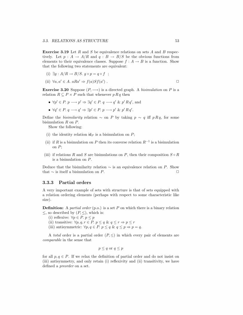
3.3. RELATIONS AS STRUCTURE 53
Exercise 3.19 Let R and S be equivalence relations on sets A and B respec-tively. Let p : A → A/R and q : B → B/S be the obvious functions fromelements to their equivalence classes. Suppose f : A → B is a function. Showthat the following two statements are equivalent:
(i) ∃g : A/R→ B/S. g ◦ p = q ◦ f ;
(ii) ∀a, a′ ∈ A. aRa′ ⇒ f(a)Sf(a′) . 2
Exercise 3.20 Suppose (P,−→) is a directed graph. A bisimulation on P is arelation R ⊆ P × P such that whenever pR q then
• ∀p′ ∈ P. p −→ p′ ⇒ ∃q′ ∈ P. q −→ q′ & p′Rq′, and
• ∀q′ ∈ P. q −→ q′ ⇒ ∃p′ ∈ P. p −→ p′ & p′Rq′.
Define the bisimilarity relation ∼ on P by taking p ∼ q iff pR q, for somebisimulation R on P .
Show the following:
(i) the identity relation idP is a bisimulation on P ;
(ii) if R is a bisimulation on P then its converse relation R−1 is a bisimulationon P ;
(iii) if relations R and S are bisimulations on P , then their composition S ◦Ris a bisimulation on P .
Deduce that the bisimilarity relation ∼ is an equivalence relation on P . Showthat ∼ is itself a bisimulation on P . 2
3.3.3 Partial orders
A very important example of sets with structure is that of sets equipped witha relation ordering elements (perhaps with respect to some characteristic likesize).
Definition: A partial order (p.o.) is a set P on which there is a binary relation≤, so described by (P,≤), which is:
(i) reflexive: ∀p ∈ P. p ≤ p(ii) transitive: ∀p, q, r ∈ P. p ≤ q & q ≤ r ⇒ p ≤ r(iii) antisymmetric: ∀p, q ∈ P. p ≤ q & q ≤ p⇒ p = q.
A total order is a partial order (P,≤) in which every pair of elements arecomparable in the sense that
p ≤ q or q ≤ p
for all p, q ∈ P . If we relax the definition of partial order and do not insist on(iii) antisymmetry, and only retain (i) reflexivity and (ii) transitivity, we havedefined a preorder on a set.
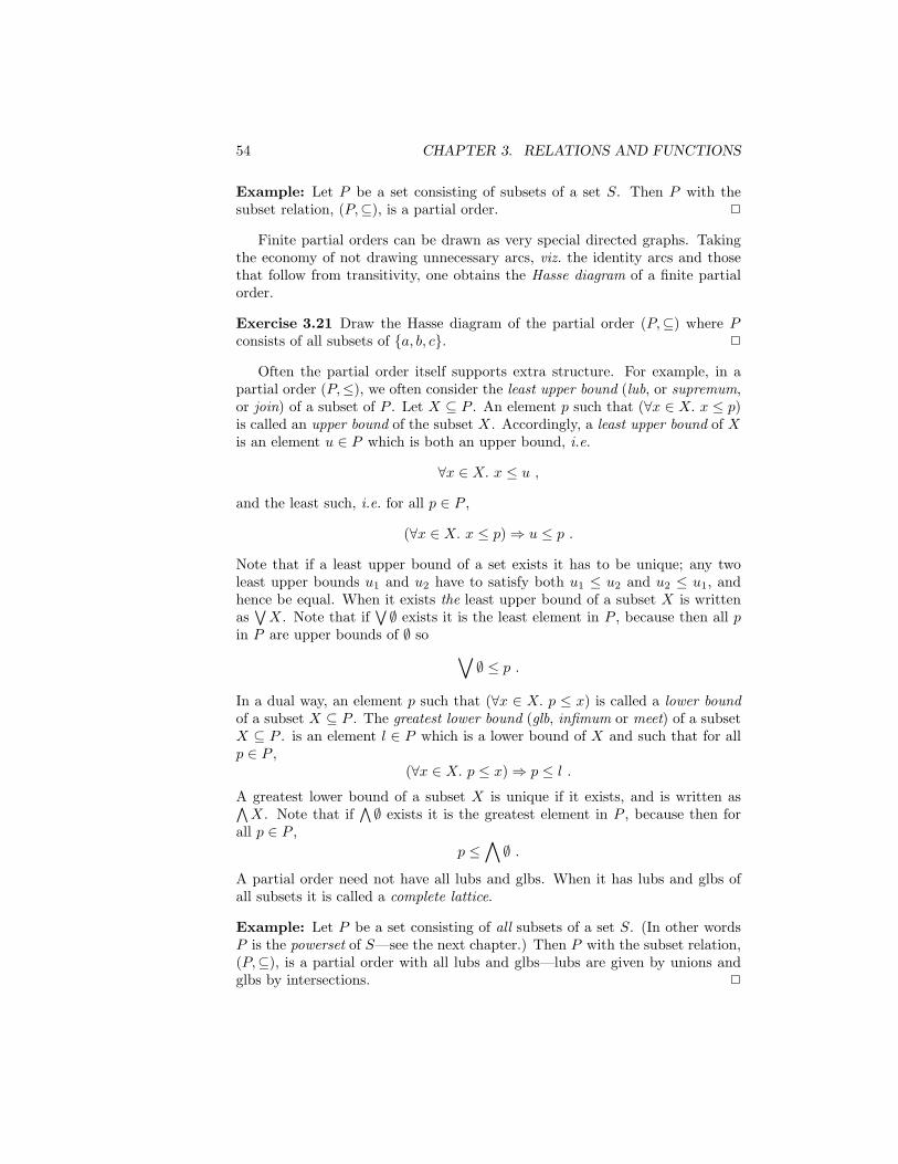
54 CHAPTER 3. RELATIONS AND FUNCTIONS
Example: Let P be a set consisting of subsets of a set S. Then P with thesubset relation, (P,⊆), is a partial order. 2
Finite partial orders can be drawn as very special directed graphs. Takingthe economy of not drawing unnecessary arcs, viz. the identity arcs and thosethat follow from transitivity, one obtains the Hasse diagram of a finite partialorder.
Exercise 3.21 Draw the Hasse diagram of the partial order (P,⊆) where Pconsists of all subsets of {a, b, c}. 2
Often the partial order itself supports extra structure. For example, in apartial order (P,≤), we often consider the least upper bound (lub, or supremum,or join) of a subset of P . Let X ⊆ P . An element p such that (∀x ∈ X. x ≤ p)is called an upper bound of the subset X. Accordingly, a least upper bound of Xis an element u ∈ P which is both an upper bound, i.e.
∀x ∈ X. x ≤ u ,
and the least such, i.e. for all p ∈ P ,
(∀x ∈ X. x ≤ p)⇒ u ≤ p .
Note that if a least upper bound of a set exists it has to be unique; any twoleast upper bounds u1 and u2 have to satisfy both u1 ≤ u2 and u2 ≤ u1, andhence be equal. When it exists the least upper bound of a subset X is writtenas∨X. Note that if
∨∅ exists it is the least element in P , because then all p
in P are upper bounds of ∅ so ∨∅ ≤ p .
In a dual way, an element p such that (∀x ∈ X. p ≤ x) is called a lower boundof a subset X ⊆ P . The greatest lower bound (glb, infimum or meet) of a subsetX ⊆ P . is an element l ∈ P which is a lower bound of X and such that for allp ∈ P ,
(∀x ∈ X. p ≤ x)⇒ p ≤ l .
A greatest lower bound of a subset X is unique if it exists, and is written as∧X. Note that if
∧∅ exists it is the greatest element in P , because then for
all p ∈ P ,p ≤
∧∅ .
A partial order need not have all lubs and glbs. When it has lubs and glbs ofall subsets it is called a complete lattice.
Example: Let P be a set consisting of all subsets of a set S. (In other wordsP is the powerset of S—see the next chapter.) Then P with the subset relation,(P,⊆), is a partial order with all lubs and glbs—lubs are given by unions andglbs by intersections. 2
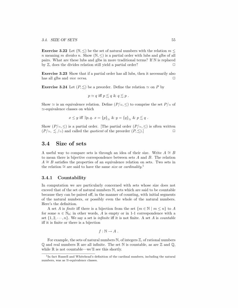
3.4. SIZE OF SETS 55
Exercise 3.22 Let (N,≤) be the set of natural numbers with the relation m ≤n meaning m divides n. Show (N,≤) is a partial order with lubs and glbs of allpairs. What are these lubs and glbs in more traditional terms? If N is replacedby Z, does the divides relation still yield a partial order? 2
Exercise 3.23 Show that if a partial order has all lubs, then it necessarily alsohas all glbs and vice versa. 2
Exercise 3.24 Let (P,.) be a preorder. Define the relation ' on P by
p ' q iff p . q & q . p .
Show ' is an equivalence relation. Define (P/',≤) to comprise the set P/' of'-equivalence classes on which
x ≤ y iff ∃p, q. x = {p}' & y = {q}' & p . q .
Show (P/',≤) is a partial order. [The partial order (P/',≤) is often written(P/', . /') and called the quotient of the preorder (P,.).] 2
3.4 Size of sets
A useful way to compare sets is through an idea of their size. Write A ∼= Bto mean there is bijective correspondence between sets A and B. The relationA ∼= B satisfies the properties of an equivalence relation on sets. Two sets inthe relation ∼= are said to have the same size or cardinality.1
3.4.1 Countability
In computation we are particularly concerned with sets whose size does notexceed that of the set of natural numbers N, sets which are said to be countablebecause they can be paired off, in the manner of counting, with initial segmentsof the natural numbers, or possibly even the whole of the natural numbers.Here’s the definition.
A set A is finite iff there is a bijection from the set {m ∈ N | m ≤ n} to Afor some n ∈ N0; in other words, A is empty or in 1-1 correspondence with aset {1, 2, · · · , n}. We say a set is infinite iff it is not finite. A set A is countableiff it is finite or there is a bijection
f : N→ A .
For example, the sets of natural numbers N, of integers Z, of rational numbersQ and real numbers R are all infinite. The set N is countable, as are Z and Q,while R is not countable—we’ll see this shortly.
1In fact Russell and Whitehead’s definition of the cardinal numbers, including the naturalnumbers, was as ∼=-equivalence classes.
56 CHAPTER 3. RELATIONS AND FUNCTIONS
Lemma 3.25 Any subset of natural numbers is countable.
Proof. Let A be a subset of N. Define a partial function f : N ⇀ A by taking
• f(1) to be the least number in A if A is nonempty and undefined otherwise,and
• f(n + 1), where n ∈ N, to be the least number in A which is larger thanf(n) if f(n) is defined and there is a member of A larger that f(n); andto be undefined otherwise.
This definition of f is an example of definition by mathematical induction: wefirst define the basis of the definition by induction, f(1), and then the inductionstep of the definition by induction, defining f(n+ 1) in terms of f(n).
From the definition of f it is clear that if f(n+ 1) is defined, then so is f(n)and f(n) < f(n+1), for all n ∈ N. It follows that if n < n′ and f(n′) is defined,then f(n) is defined and f(n) < f(n′). Hence
D = {n ∈ N | f(n) is defined}
is either N, or of the form {n ∈ N | n ≤ m}, a finite initial segment of the naturalnumbers. Furthermore f : D → A is injective as two distinct elements of D willbe strictly ordered so have distinct images under f .
To show f is also surjective, suppose otherwise. Then there would be a leasta ∈ A not in the image fD. The element a cannot be the least element of Abecause this least element is f(1), clearly in fD. So there must be a largestelement a′ of A such that a′ < a. Because a′ < a there is n ∈ D such thatf(n) = a′. But then f(n+ 1) = a—contradiction. 2
Corollary 3.26 A set B is countable iff there is a bijection g : A → B fromA ⊆ N.
Proof. “only if”: follows directly from the definition of countability. “if”: ByLemma 3.25 a subset A ⊆ N is countable so there is a bijection f : D → A whereD is a finite initial segment or the whole of N. The composition g ◦ f : D → Bis a bijection establishing the countability of B. 2
In establishing countability of a set we do not need to be so demanding asCorollary 3.26; an injection from the set into the natural numbers suffices:
Lemma 3.27 A set B is countable iff there is an injection f : B → N.
Proof. “only if”: Assuming B is countable there is a bijection g : A→ B fromA ⊆ N by Corollary 3.26. The function g has an inverse function g−1 : B → A,by Lemma 3.9. Let j;A→ N be the inclusion function. Then f = j ◦g−1 : B →N is an injection, being the composition of two injections. “if”: An injectionf : B → N becomes a bijection f : B → f B because f regarded as a functionfrom B to the direct image f B is clearly both injective and surjective. Now itsinverse f−1 : f B → B is a bijection from f B ⊆ N. Hence by Corollary 3.26the set B is countable. 2
3.4. SIZE OF SETS 57
So, a set is countable iff there is an injection from it into the natural numbers.We could instead have taken this as our definition of countability. Thoughour current definition has the advantage of being more customary and directlyrelated to our intuitions about counting. As we will see, the following fact,a slight relaxation of Lemma 3.27, is often useful in establishing that a set iscountable.
Lemma 3.28 A set B is countable iff there is an injection f : B → A into aset A which is countable.
Proof. “only if”: If B is countable, then there is an injection f : B → N byLemma 3.27, and N is countable. (Alternatively, if B is countable, then certainlyidB : B → B is an injection into a countable set.) “if”: Suppose f : B → Ais an injection and the set A is countable. Then, by Lemma 3.27, there is aninjection h : A → N. It follows that the composition g = h ◦ f : B → N is aninjection. So, again by Lemma 3.27, the set B is countable. 2
Notice that if B ⊆ A then there is an inclusion function from B to A takingb ∈ B to b ∈ A—the inclusion function is clearly injective. So Lemma 3.28specialises to say a set B is countable iff it is included in a countable set A.
Lemma 3.29 The set N× N is countable.
Proof. The function f : N× N→ N defined by
f(m,n) = 2m × 3n
is an injection into a countable set. By Lemma 3.28, N× N is countable. 2
Corollary 3.30 The set of positive rational numbers Q+ is countable.
Proof. Any positive rational q can be written uniquely as a fraction mq/nqwhere mq and nq are natural numbers with no common factor. Define a functionf : Q+ → N×N by taking f(q) = (mq, nq). Then f is an injection—two differentrationals determine different fractions. So Q+ is countable by Lemma 3.28. 2
Corollary 3.31 If A and B are countable sets, then so is their product A×B.
Proof. Assume sets A and B are countable. Then there are injections fA :A → N and fB : B → N, by Lemma 3.28. We can combine them into anlnjection f : A×B → N× N by defining f(a, b) = (fA(a), fB(b)). We spell outthe easy check that f is an injection, which uses standard properties of pairsand that fA and fB are injections. Let (a, b) and (a′, b′) be pairs in A × B forwhich f(a, b) = f(a′, b′). We obtain (fA(a), fB(b)) = (fA(a′), fB(b′)). Whence,fA(a) = fA(a′) and fB(b) = fB(b′). So a = a′ and b = b′ by the injectivity offA and fB . Thus (a, b) = (a′, b′). 2
58 CHAPTER 3. RELATIONS AND FUNCTIONS
We have seen unions, like A1 ∪ A2 ∪ · · · ∪ Ak, of finitely sets A1, · · · , Ak.Imagine now that we are given an infinite sequence of sets A1, A2, A3, · · · , An, · · ·indexed by the natural numbers. We can also form their union; we might writethat union as
A1 ∪A2 ∪A3 ∪ · · ·An ∪ · · ·
though this perhaps makes the union seem more mysterious than it is, becauseit suggests wrongly a form of limiting process like those in real or complexanalysis. A better way to write the union of the sequence of sets is as⋃
n∈NAn =def {x | ∃n ∈ N. x ∈ An} ,
which exposes how innocent this union of countably many sets really is. Thenext lemma shows that if each of the sets An is countable then so is theirunion. The lemma is often expressed as: a countable union of countable sets iscountable.
Lemma 3.32 Suppose A1, A2, · · · , An, · · · are all countable sets. Their union⋃n∈N An is countable.
Proof. Write A for the set⋃n∈N An. By Lemma 3.27, for each n there is an
injection fn : An → N. Define an injection h : A→ N×N as follows. For x ∈ A,let nx be the least number for which x ∈ Anx , and take
h(x) = (nx, fnx(x)) .
We check that h is an injection: Suppose h(x) = h(y) for x, y ∈ A. Thennx = ny so x, y ∈ Anx and fnx(x) = fnx(y). But fnx is injective, so x = y.Hence A is countable by Lemmas 3.28 and 3.29. 2
Notice thay the above lemma also applies to finite unions, because the An’scould all be the empty set from some point on.
Exercise 3.33 Prove that the set Z of integers and the set Q of all rationalnumbers are countable. [Both proofs involve the same idea.] 2
Exercise 3.34 Show that the set of all finite subsets of N is countable. 2
Exercise 3.35 Show that Q×Q is countable. Deduce that any set of disjointdiscs (i.e. circular areas which may or may not include their perimeter) in theplane R × R is countable. Is the same true if “discs” is replaced by “circles”(i.e. just the perimeters of the circles)? 2
Exercise 3.36 Show that a nonempty set A is countable iff there is a surjectionf : N→ A. 2
3.4. SIZE OF SETS 59
3.4.2 Uncountability
Not all sets are countable. One of the notable mathematical accomplishments ofthe 19th century was Georg Cantor’s proof that the set of real numbers R is un-countable, i.e. not countable. This opened up new ways to prove the existenceof certain kinds of real numbers. His second, simpler proof of the uncount-ability of R used a diagonal argument, a style of argument which reappears inshowing the undecidability of the halting problem, is implicit in the proof ofGodel’s incompleteness theorem, and can sometimes be used in establishing thehierarchies of complexity theory.
Theorem 3.37 The set of real numbers R is uncountable.
Proof. The proof is by contradiction. Assume that R is countable. Then byLemma 3.28, the interval (0, 1] = {r ∈ R | 0 < r ≤ 1} ⊆ R will also be a count-able set. Each number in (0, 1] is represented uniquely by a non-terminatingdecimal expansion; for example 0.13 is represented by the non-terminating dec-imal 0.12999 · · ·. The set (0, 1] is clearly infinite (any finite set of reals wouldcontain a least element, which (0, 1] clearly does not). So (0, 1] being countableimplies there is a bijection f : N→ (0, 1]. Write
f(n) = 0.dn1dn2d
n3 · · · dni · · ·
to describe the non-terminating decimal expansion of the nth real in the enu-meration given by f . We’ll produce a number r in (0, 1] which can’t be in theenumeration, so yielding a contradiction. Define the number’s decimal expan-sion to be
0.r1r2r3 · · · ri · · ·
where
ri ={
1 if dii 6= 1,2 if dii = 1 .
Clearly r ∈ (0, 1]. Thus there is some natural number k such that f(k) =r. Hence by the uniqueness of the decimal expansions ri = dki for all i. Inparticular,
rk = dkk .
But, from the definition of rk, we have that rk = 1 if dkk 6= 1, and rk = 2 ifdkk = 1. In either case, rk 6= dkk—a contradiction.
We conclude that the original assumption, that R is countable, is false. 2
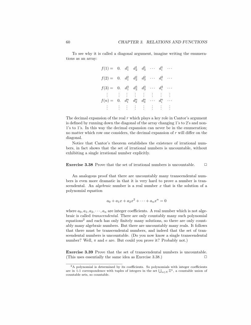
60 CHAPTER 3. RELATIONS AND FUNCTIONS
To see why it is called a diagonal argument, imagine writing the enumera-tions as an array:
f(1) = 0. d11 d1
2 d13 · · · d1
i · · ·
f(2) = 0. d21 d2
2 d23 · · · d2
i · · ·
f(3) = 0. d31 d3
2 d33 · · · d3
i · · ·...
......
......
......
...f(n) = 0. dn1 dn2 dn3 · · · dni · · ·
......
......
......
......
The decimal expansion of the real r which plays a key role in Cantor’s argumentis defined by running down the diagonal of the array changing 1’s to 2’s and non-1’s to 1’s. In this way the decimal expansion can never be in the enumeration;no matter which row one considers, the decimal expansion of r will differ on thediagonal.
Notice that Cantor’s theorem establishes the existence of irrational num-bers, in fact shows that the set of irrational numbers is uncountable, withoutexhibiting a single irrational number explicitly.
Exercise 3.38 Prove that the set of irrational numbers is uncountable. 2
An analogous proof that there are uncountably many transcendental num-bers is even more dramatic in that it is very hard to prove a number is tran-scendental. An algebraic number is a real number x that is the solution of apolynomial equation
a0 + a1x+ a2x2 + · · ·+ anx
n = 0
where a0, a1, a2, · · · , an are integer coefficients. A real number which is not alge-braic is called transcendental. There are only countably many such polynomialequations2 and each has only finitely many solutions, so there are only count-ably many algebraic numbers. But there are uncountably many reals. It followsthat there must be transcendental numbers, and indeed that the set of tran-scendental numbers is uncountable. (Do you now know a single transcendentalnumber? Well, π and e are. But could you prove it? Probably not.)
Exercise 3.39 Prove that the set of transcendental numbers is uncountable.(This uses essentially the same idea as Exercise 3.38.) 2
2A polynomial is determined by its coefficients. So polynomials with integer coefficientsare in 1-1 correspondence with tuples of integers in the set
Sn∈N Zn, a countable union of
countable sets, so countable.
3.4. SIZE OF SETS 61
Investigating cardinality
By Lemma 3.28, if f : B → A is an injection and A is countable, then so is B.So, when investigating cardinality,
• to show a set B is countable it suffices to exhibit an injection from B setinto a set A known to be countable; while
• to show a set A is uncountable it suffices to exhibit an injection from a setB known to be uncountable into A. Because then, if A were countable, sowould B be countable—a contradiction.
Sometimes (though rarely in undergraduate courses) we need to investigatecardinality beyond countability or its failure. Then the key tool is the Schroder-Bernstein theorem.This says that two sets A and B have the same cardinality iffthere are injections f : A→ B and g : B → A. The hard part of its proof showshow to construct a bijection between A and B out of the two injections—seeExercise ??.
Exercise 3.40 By using a variation on the diagonal argument above, show thatthe powerset, P(N) =def {S | S ⊆ N}, is uncountable. (See Section 4.3.2 for aproof.) 2
Exercise 3.41 Which of the following sets are finite, which are infinite butcountable, and which are uncountable?
• {f : N→ {0, 1} | ∀n ∈ N. f(n) ≤ f(n+ 1)}
• {f : N→ {0, 1} | ∀n ∈ N. f(2n) 6= f(2n+ 1)}
• {f : N→ {0, 1} | ∀n ∈ N. f(n) 6= f(n+ 1)}
• {f : N→ N | ∀n ∈ N. f(n) ≤ f(n+ 1)}
• {f : N→ N | ∀n ∈ N. f(n) ≥ f(n+ 1)}
2
Exercise 3.42 (Schroder-Bernstein theorem) Let f : A→ B and g : B → A beinjections between two sets A and B. Note that the function g : B → g B is a bi-jection, with inverse function g−1 : g B → B. Define subsets C1, C2, · · · , Cn, · · ·of A by the following induction:
C1 = A \ (g B)Cn+1 = (g ◦ f)Cn
.
Define C =⋃n∈N Cn. Now define a function h : A→ B by
h(a) = f(a) if a ∈ C,h(a) = g−1(a) if a /∈ C
62 CHAPTER 3. RELATIONS AND FUNCTIONS
—if a /∈ C then a ∈ g B, so it makes sense to apply g−1 to a /∈ C.Prove h is a bijection from A to B by showing:
(i) h is injective: Show if a ∈ C and a′ /∈ C, then h(a) 6= h(a′). Deduce that his injective.(ii) h is surjective: Show (g ◦ f)C = C \ C1. Whence, or otherwise, show thatif g(b) ∈ C then b ∈ f C. Deduce, if b /∈ f C then g(b) /∈ C, and hence that h issurjective. 2
Chapter 4
Constructions on sets
Forewarned by a problem first exposed by Bertrand Russell, we look to safemethods for constructing sets.
4.1 Russell’s paradox
When set theory was being invented it was thought, first of all, that any propertyP (x) determined a set
{x | P (x)} .It came as a shock when Bertrand Russell realised that assuming the existenceof certain sets described in this way gave rise to contradictions.1
Russell’s paradox is really the demonstration that a contradiction arises fromthe liberal way of constructing sets above. His argument proceeds as follows.Consider the property
x /∈ xa way of writing “x is not an element of x.” If we assume that propertiesdetermine sets, just as described, we can form the set
R = {x | x /∈ x} .
Either R ∈ R or not. If so, i.e. R ∈ R, then in order for R to qualify as anelement of R, from the definition of R, we deduce R /∈ R. So we end up assertingboth something and its negation—a contradiction. If, on the other hand, R /∈ Rthen from the definition of R we see R ∈ R—a contradiction again. EitherR ∈ R or R /∈ R lands us in trouble.
We need to have some way which stops us from considering a collection likeR as a set, and so as a legitimate element. In general terms, the solution is to
1The shock was not just to Russell and his collaborator Alfred North Whitehead. GottlobFrege received the news as his book on the foundations of mathematics via sets was beingprinted—the paradox was devastating for his work. Some were delighted however. The greatmathematician Henri Poincare is reported as gleefully saying “Logic is not barren, it’s broughtforth a paradox!” Apparently, Georg Cantor already knew of Russell’s paradox.
63
64 CHAPTER 4. CONSTRUCTIONS ON SETS
discipline the way in which sets are constructed, so that starting from certaingiven sets, new sets can only be formed when they are constructed by usingparticular, safe ways from old sets. We shall state those sets we assume to existright from the start and methods we allow for constructing new sets. Providedthese are followed we avoid trouble like Russell’s paradox and at the same timehave a rich enough world of sets to support most mathematics.2
4.2 Constructing sets
4.2.1 Basic sets
We take the existence of the empty set ∅ for granted, along with certain sets ofbasic elements such as
N0 = {0, 1, 2, · · ·} .
We shall also take sets of symbols like
{“a”, “b”, “c”, “d”, “e”, · · · , “z”}
for granted, although we could, alternatively have represented them as particularnumbers for example, or even as certain sets. The equality relation on a set ofsymbols is that given by syntactic identity written ≡. Two symbols are equaliff they are literally the same.
4.2.2 Constructions
We shall take for granted certain operations on sets which enable us to constructsets from given sets.
Comprehension
If X is a set and P (x) is a property, we can form the set
{x ∈ X | P (x)} ,
the subset of X consisting of all elements x of X which satisfy P (x).Sometimes we’ll use a further abbreviation. Suppose e(x1, . . . , xn) is some
expression which for particular elements x1 ∈ X1, · · ·xn ∈ Xn yields a particularelement and P (x1, . . . , xn) is a property of such x1, . . . , xn. We use
{e(x1, . . . , xn) | x1 ∈ X1 & · · ·& xn ∈ Xn & P (x1, . . . , xn)}
to abbreviate
{y | ∃x1 ∈ X1, · · · , xn ∈ Xn. y = e(x1, . . . , xn)& P (x1, . . . , xn)} .2Occasionally we consider collections which are not sets. For example, it can be useful to
consider the collection of all sets. But such a collection is not itself a set, so cannot be madea proper element of any collection. The word ‘class’ which originally was synonymous with‘set’ is now generally reserved for a collection which need not necessarily be a set.
4.2. CONSTRUCTING SETS 65
For example,{2m+ 1 | m ∈ N & m > 1}
is the set of odd numbers greater than 3.
Remark Note a consequence of comprehension. The collection {x | x is a set }is not itself a set. If it were then by using comprehension Russell’s collectionR would be a set, which is contradictory in the manner of Russell’s originalargument. As the collection of all sets is not a set we fortunately side-stephaving to consider whether it is a member of itself. 2
Powerset
We can form a set consisting of the set of all subsets of a set, the so-calledpowerset:
P(X) = {Y | Y ⊆ X}.This is the important construction for building bigger sets. We shall see shortlythat a powerset P(X) always has larger size than X.
Exercise 4.1 Let B be a fixed subset of the set A. Define the relation R onP(A) by
(X,Y ) ∈ R ⇐⇒ X ∩B = Y ∩B .
Show that R is an equivalence relation and describe a bijection between the setof R-equivalence classes and P(B). 2
Unordered pairs
A seemingly modest but important way to produce sets is through formingunordered pairs. Given two objects x and y—they might be sets—we can formthe set {x, y} whose sole elements are x and y.
Indexed sets
Suppose I is a set and that for any i ∈ I there is a unique object xi, maybe aset itself. Then
{xi | i ∈ I}is a set. The elements xi are said to be indexed by the elements i ∈ I. Anycollection of objects indexed by a set is itself a set.
Union
As we’ve seen, the set consisting of the union of two sets has as elements thoseelements which are either elements of one or the other set:
X ∪ Y = {a | a ∈ X or a ∈ Y }.
This union is an instance of a more general construction, “big union,” that wecan perform on any set of sets.
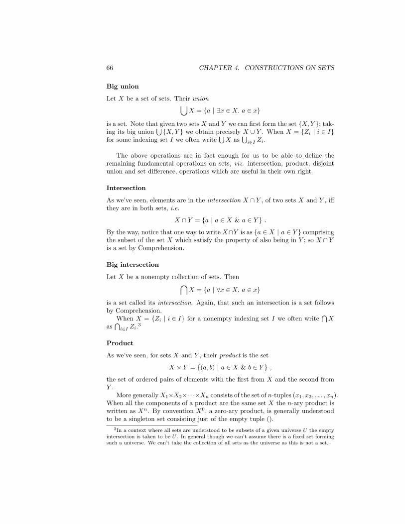
66 CHAPTER 4. CONSTRUCTIONS ON SETS
Big union
Let X be a set of sets. Their union⋃X = {a | ∃x ∈ X. a ∈ x}
is a set. Note that given two sets X and Y we can first form the set {X,Y }; tak-ing its big union
⋃{X,Y } we obtain precisely X ∪ Y . When X = {Zi | i ∈ I}
for some indexing set I we often write⋃X as
⋃i∈I Zi.
The above operations are in fact enough for us to be able to define theremaining fundamental operations on sets, viz. intersection, product, disjointunion and set difference, operations which are useful in their own right.
Intersection
As we’ve seen, elements are in the intersection X ∩ Y , of two sets X and Y , iffthey are in both sets, i.e.
X ∩ Y = {a | a ∈ X & a ∈ Y } .
By the way, notice that one way to write X∩Y is as {a ∈ X | a ∈ Y } comprisingthe subset of the set X which satisfy the property of also being in Y ; so X ∩ Yis a set by Comprehension.
Big intersection
Let X be a nonempty collection of sets. Then⋂X = {a | ∀x ∈ X. a ∈ x}
is a set called its intersection. Again, that such an intersection is a set followsby Comprehension.
When X = {Zi | i ∈ I} for a nonempty indexing set I we often write⋂X
as⋂i∈I Zi.
3
Product
As we’ve seen, for sets X and Y , their product is the set
X × Y = {(a, b) | a ∈ X & b ∈ Y } ,
the set of ordered pairs of elements with the first from X and the second fromY .
More generallyX1×X2×· · ·×Xn consists of the set of n-tuples (x1, x2, . . . , xn).When all the components of a product are the same set X the n-ary product iswritten as Xn. By convention X0, a zero-ary product, is generally understoodto be a singleton set consisting just of the empty tuple ().
3In a context where all sets are understood to be subsets of a given universe U the emptyintersection is taken to be U . In general though we can’t assume there is a fixed set formingsuch a universe. We can’t take the collection of all sets as the universe as this is not a set.
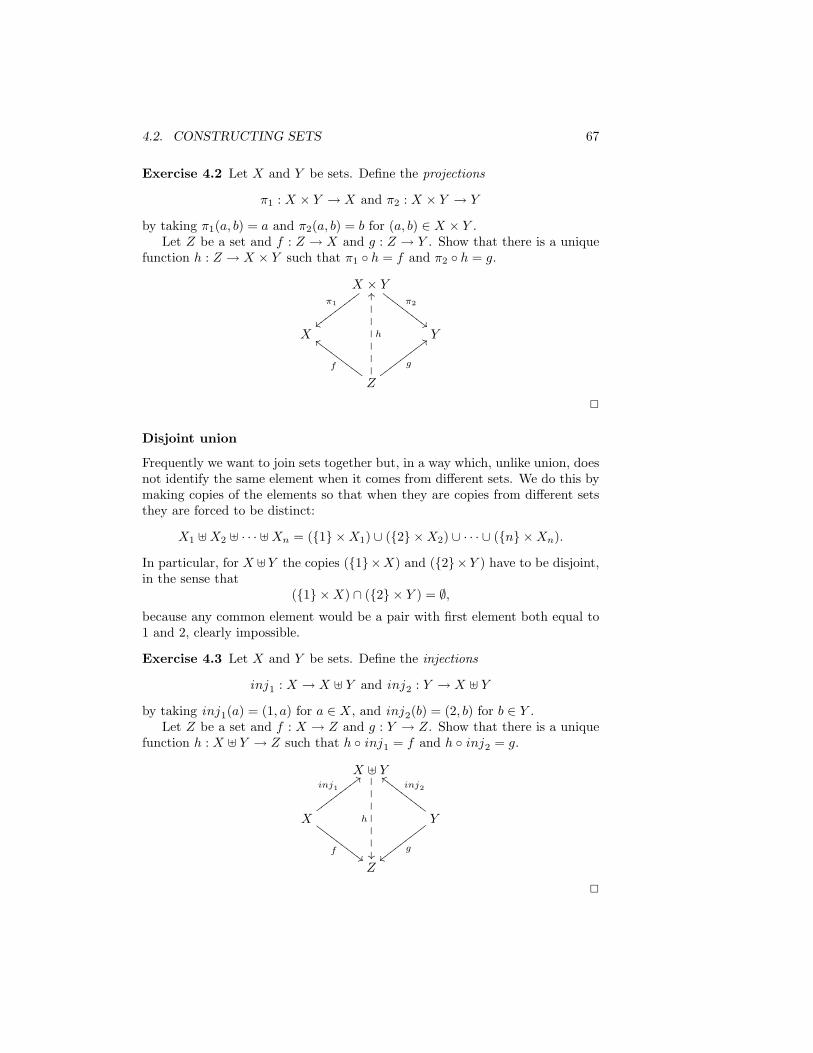
4.2. CONSTRUCTING SETS 67
Exercise 4.2 Let X and Y be sets. Define the projections
π1 : X × Y → X and π2 : X × Y → Y
by taking π1(a, b) = a and π2(a, b) = b for (a, b) ∈ X × Y .Let Z be a set and f : Z → X and g : Z → Y . Show that there is a unique
function h : Z → X × Y such that π1 ◦ h = f and π2 ◦ h = g.
X × Yπ1
{{wwwwwwwwwπ2
##GGGGGGGGG
X Y
Z
f
ccGGGGGGGGG
h
OO������� g
;;wwwwwwwww
2
Disjoint union
Frequently we want to join sets together but, in a way which, unlike union, doesnot identify the same element when it comes from different sets. We do this bymaking copies of the elements so that when they are copies from different setsthey are forced to be distinct:
X1 ]X2 ] · · · ]Xn = ({1} ×X1) ∪ ({2} ×X2) ∪ · · · ∪ ({n} ×Xn).
In particular, for X ]Y the copies ({1}×X) and ({2}×Y ) have to be disjoint,in the sense that
({1} ×X) ∩ ({2} × Y ) = ∅,because any common element would be a pair with first element both equal to1 and 2, clearly impossible.
Exercise 4.3 Let X and Y be sets. Define the injections
inj1 : X → X ] Y and inj2 : Y → X ] Y
by taking inj1(a) = (1, a) for a ∈ X, and inj2(b) = (2, b) for b ∈ Y .Let Z be a set and f : X → Z and g : Y → Z. Show that there is a unique
function h : X ] Y → Z such that h ◦ inj1 = f and h ◦ inj2 = g.
X ] Y
h
���������
X
f##GGGGGGGGG
inj1
;;wwwwwwwwwY
inj2
ccGGGGGGGGG
g{{xxxxxxxxx
Z
2
68 CHAPTER 4. CONSTRUCTIONS ON SETS
Set difference
We can subtract one set Y from another X, an operation which removes allelements from X which are also in Y .
X \ Y = {x | x ∈ X & x /∈ Y } .
4.2.3 Axioms of set theory
The constructions we have described include most of the assumptions madein more axiomatic treatments of set theory based on the work of Zermelo andFrænkel. To spell out the connection, the existence of the set of natural numbers,powersets, unordered pairs, big unions and sets of indexed objects correspond tothe axioms of infinity, powerset, pairing, union and replacement respectively; wehave adopted the axiom of comprehension directly, and the axiom of extension-ality amounts to saying a set is determined by its elements. For completenesswe mention two remaining axioms, the axiom of foundation and the axiom ofchoice, which are generally assumed of sets. While sensible and safe axioms toassume of sets, they do not in fact follow from the constructions we have givenso far.
The axiom of foundation
A set is built-up starting from basic sets by using the constructions described.We remark that a property of sets, called the axiom of foundation, follows fromour informal understanding of sets and how we can construct them. Consideran element b1 of a set b0. It is either a basic element, like an integer or a symbol,or it is a set. If b1 is a set then it must have been constructed from sets whichhave themselves been constructed earlier. Intuitively, we expect any chain ofmemberships
· · · bn ∈ · · · ∈ b1 ∈ b0
to end in some bn which is some basic element or the empty set. The statementthat any such descending chain of memberships must be finite is called theaxiom of foundation, and is an assumption generally made in set theory. Noticethe axiom implies that no set X can be a member of itself as, if this were so,we’d get the infinite descending chain
· · ·X ∈ · · · ∈ X ∈ X
—a contradiction.
General products and the axiom of choice
Occasionally it is important to have a general form of product in which insteadof pairs with first and second coordinates, or finite tuples, we have tuples where
4.3. SOME CONSEQUENCES 69
the coordinates correspond to indices in a general set I. Let Xi be a set foreach element i in a set I. By definition the general product∏
i∈IXi = {f : I →
⋃i∈I
Xi | ∀i ∈ I. f(i) ∈ Xi} .
Given f ∈∏i∈I Xi we can get the ith coordinate as f(i). Given xi ∈ Xi for each
i ∈ I, we can form their tuple f ∈∏i∈I Xi by defining f(i) = xi for all i ∈ I.
It’s not too hard to construct the set∏i∈I Xi out of the earlier constructions.
Is the set∏i∈I Xi nonempty? It has to be empty if Xi = ∅ for any i ∈ I. But
if Xi is nonempty for every i ∈ I it would seem reasonable that one could makea function f ∈
∏i∈I Xi by choosing some f(i) ∈ Xi for all i ∈ I. When I is a
finite set it is easy to make such a tuple, and so prove that∏i∈I Xi is nonempty
if each Xi is. For a while it was thought that this perfectly reasonable propertywas derivable from more basic axioms even when I is infinite. However, thisturns out not to be so. Occasionally one must have recourse to the axiom ofchoice which says provided each Xi is nonempty for i ∈ I, then so is the product∏i∈I Xi.
Exercise 4.4 Show that the axiom of choice can be reformulated as the follow-ing: for every surjection g : A → B there is an injection f : B → A such thatg ◦ f = idB . 2
Exercise 4.5 Show, using the axiom of choice and the Schroder-Bernstein the-orem (Exercise ??), that two sets A and B have the same size (i.e. there is abijection between them) if there is both an injection f : A→ B and a surjectiong : A→ B. 2
4.3 Some consequences
4.3.1 Sets of functions
The set of all relations between sets X and Y is the set P(X × Y ). Usingcomprehension it is then easy to see that
(X ⇀ Y ) = {f ∈ P(X × Y ) | f is a partial function}
is a set; that of all partial functions from X to Y . Similarly,
(X → Y ) = {f ∈ P(X × Y ) | f is a function}
is also a set; that of all total functions from X to Y . Often this set is writtenY X .
Exercise 4.6 Let A2 = {1, 2} and A3 = {a, b, c}. List the elements of the foursets (Ai → Aj) for i, j ∈ {2, 3}. Annotate those elements which are injections,surjections and bijections. 2
70 CHAPTER 4. CONSTRUCTIONS ON SETS
Exercise 4.7 Let X and Y be sets. Show there is a bijection between the setof functions (X → P(Y )) and the set of relations P(X × Y ). 2
When investigating the behaviour of a function f ∈ (X → Y ) we applyit to arguments. Earlier in Proposition 3.3 we saw that equality of functionsf, f ′ ∈ (X → Y ) amounts to their giving the same result on an arbitraryargument x in X. We can treat functions as sets and so might introduce afunction by describing the property satisfied by its input-output pairs. But thiswould ignore the fact that a function is most often introduced as an expressione describing its output in Y in terms of its input x in X. For this manner ofdescription lambda notation (or λ-notation) is most suitable.
Lambda notation
Lambda notation provides a way to describe functions without having to namethem. Suppose f : X → Y is a function which for any element x in X gives avalue f(x) described by an expression e, probably involving x. Sometimes wewrite
λx ∈ X. e
for the function f . Thus
λx ∈ X. e = {(x, e) | x ∈ X} .
So, λx ∈ X. e is an abbreviation for the set of input-output pairs determinedby the expression e. For example, λx ∈ N0. x+ 1 is the successor function andwe have (λx ∈ N0. x+ 1) ∈ (N0 → N0).
Exercise 4.8 Use lambda notation to describe bijections
[(A×B)→ C] ∼= [A→ (B → C)] ,[A→ (B → C)] ∼= [B → (A→ C)] .
2
Exercise 4.9 Describe explicit bijections
[(A ]B)→ C] ∼= (A→ C)× (B → C),[A→ (B × C)] ∼= (A→ B)× (A→ C) .
2
Characteristic functions
In set theory one starts with sets as primitive and builds functions. We builtsets of functions (X → Y ) with the help of powersets. There are alternativefoundations of mathematics which work the other way round. They start withfunctions and “types” of functions (X → Y ) and identify sets with special
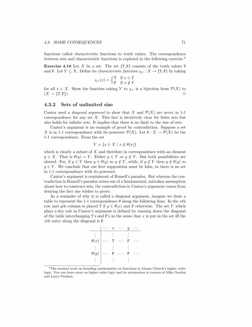
4.3. SOME CONSEQUENCES 71
functions called characteristic functions to truth values. The correspondencebetween sets and characteristic functions is explored in the following exercise.4
Exercise 4.10 Let X be a set. The set {T, F} consists of the truth values Tand F. Let Y ⊆ X. Define its characteristic function χY : X → {T, F} by taking
χY (x) ={T if x ∈ YF if x /∈ Y
for all x ∈ X. Show the function taking Y to χY is a bijection from P(X) to(X → {T, F}). 2
4.3.2 Sets of unlimited size
Cantor used a diagonal argument to show that X and P(X) are never in 1-1correspondence for any set X. This fact is intuitively clear for finite sets butalso holds for infinite sets. It implies that there is no limit to the size of sets.
Cantor’s argument is an example of proof by contradiction. Suppose a setX is in 1-1 correspondence with its powerset P(X). Let θ : X → P(X) be the1-1 correspondence. Form the set
Y = {x ∈ X | x /∈ θ(x)}
which is clearly a subset of X and therefore in correspondence with an elementy ∈ X. That is θ(y) = Y . Either y ∈ Y or y /∈ Y . But both possibilities areabsurd. For, if y ∈ Y then y ∈ θ(y) so y /∈ Y , while, if y /∈ Y then y /∈ θ(y) soy ∈ Y . We conclude that our first supposition must be false, so there is no setin 1-1 correspondence with its powerset.
Cantor’s argument is reminiscent of Russell’s paradox. But whereas the con-tradiction in Russell’s paradox arises out of a fundamental, mistaken assumptionabout how to construct sets, the contradiction in Cantor’s argument comes fromdenying the fact one wishes to prove.
As a reminder of why it is called a diagonal argument, imagine we draw atable to represent the 1-1 correspondence θ along the following lines. In the xthrow and yth column is placed T if y ∈ θ(x) and F otherwise. The set Y whichplays a key role in Cantor’s argument is defined by running down the diagonalof the table interchanging T’s and F’s in the sense that x is put in the set iff thexth entry along the diagonal is F.
· · · x · · · y · · ·...
......
θ(x) · · · T · · · F · · ·...
......
θ(y) · · · F · · · F · · ·...
......
4The seminal work on founding mathematics on functions is Alonzo Church’s higher orderlogic. You can learn more on higher order logic and its automation in courses of Mike Gordonand Larry Paulson.
72 CHAPTER 4. CONSTRUCTIONS ON SETS
Exercise 4.11 This exercise guides you through to a proof that for any sets Xand Y , with Y containing at least two elements, there cannot be an injectionfrom the set of functions (X → Y ) to X.
(i) Let X be a set. Prove there is no injection f : P(X) → X.[Hint: Consider the set W =def {f(Z) | Z ⊆ X & f(Z) /∈ Z}.]
(ii) Suppose now that a set Y has at least two distinct elements. Define aninjection k : P(X) → (X → Y ), from the powerset of X to the set offunctions from X to Y .
(iii) Prove that there is no injection from (X → Y ) to X when the set Yhas at least two distinct elements. [Hint: Recall that the composition ofinjections is an injection.]
2
Chapter 5
Inductive definitions
This chapter shows where induction principles come from. It is an introductionto the theory of inductively-defined sets. It provides general methods for definingsets recursively, and general induction rules to accompany inductively-definedsets.
5.1 Sets defined by rules—examples
Often a set is described in the following way. Some clauses stipulate that certainbasic elements are to be in the set; then clauses are given stipulating furtherelements of the set in terms of elements already included. Implicitly, only el-ements produced in these stipulated ways are to be included in the set. Thisgives a kind of recipe for making a set: first put in the basic elements; then,conditional on certain elements being in, add others. Sets described in this wayare called inductively defined.
Inductively defined sets are ubiquitous, but not always presented in thesame way. To stress the commonality in their form of definition we’ll presentinductively-defined sets via rules. A rule instance comprises its premises and aconclusion
x1, x2, · · ·y
.
The intended interpretation is: if the premises x1, x2, · · · are in the set beingdefined, then so is the conclusion y. The premises may form an empty set,in which case the rule simply expresses that the conclusion y is in the set.The following examples only give a limited idea of the range of applicationsof inductive definitions—you’ll meet them again and again, in applications asdiverse as semantics, logic, verification, logic programming, datatypes, compilerconstruction, security, probability, . . .
Example: The syntax of Boolean propositions has been described by
A, B, ... ::= a, b, c, · · · | T | F | A ∧ B | A ∨ B | ¬A
73
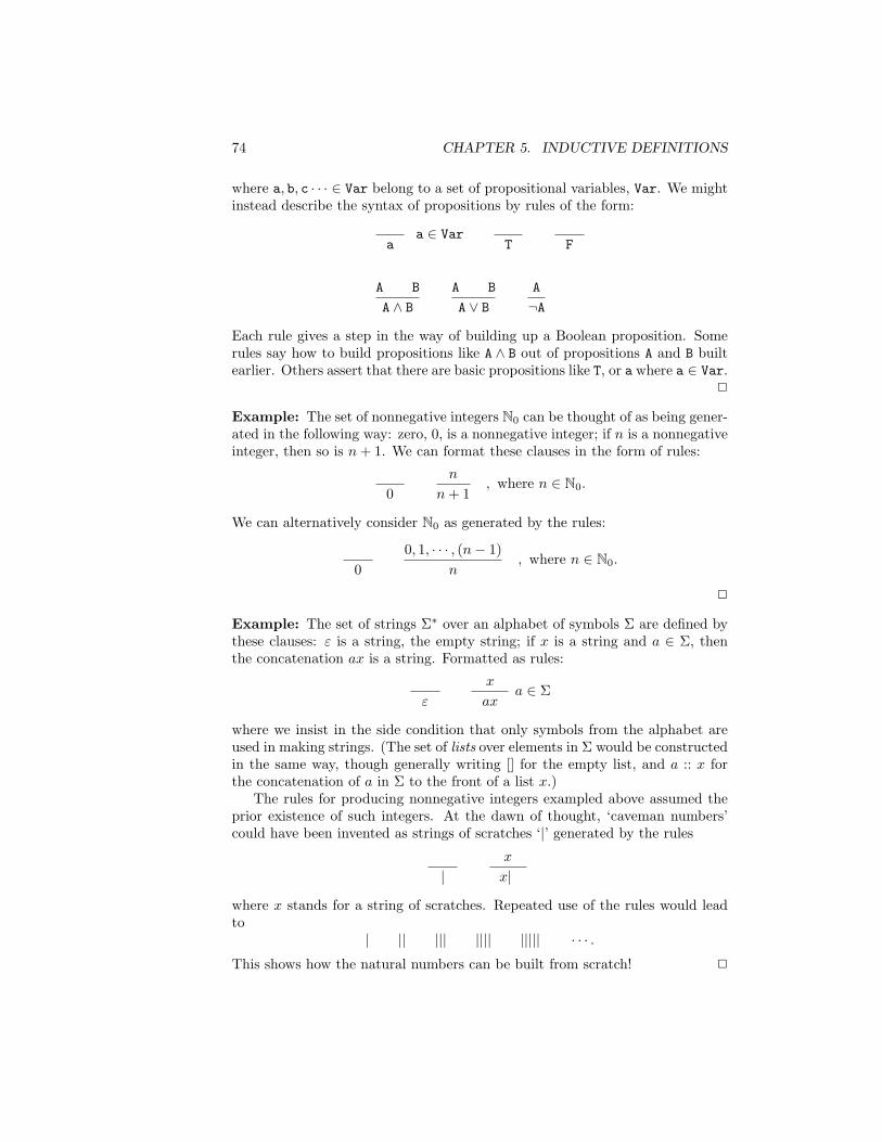
74 CHAPTER 5. INDUCTIVE DEFINITIONS
where a, b, c · · · ∈ Var belong to a set of propositional variables, Var. We mightinstead describe the syntax of propositions by rules of the form:
aa ∈ Var
T F
A B
A ∧ BA B
A ∨ BA
¬A
Each rule gives a step in the way of building up a Boolean proposition. Somerules say how to build propositions like A ∧ B out of propositions A and B builtearlier. Others assert that there are basic propositions like T, or a where a ∈ Var.
2
Example: The set of nonnegative integers N0 can be thought of as being gener-ated in the following way: zero, 0, is a nonnegative integer; if n is a nonnegativeinteger, then so is n+ 1. We can format these clauses in the form of rules:
0n
n+ 1, where n ∈ N0.
We can alternatively consider N0 as generated by the rules:
00, 1, · · · , (n− 1)
n, where n ∈ N0.
2
Example: The set of strings Σ∗ over an alphabet of symbols Σ are defined bythese clauses: ε is a string, the empty string; if x is a string and a ∈ Σ, thenthe concatenation ax is a string. Formatted as rules:
ε
x
axa ∈ Σ
where we insist in the side condition that only symbols from the alphabet areused in making strings. (The set of lists over elements in Σ would be constructedin the same way, though generally writing [] for the empty list, and a :: x forthe concatenation of a in Σ to the front of a list x.)
The rules for producing nonnegative integers exampled above assumed theprior existence of such integers. At the dawn of thought, ‘caveman numbers’could have been invented as strings of scratches ‘|’ generated by the rules
|x
x|
where x stands for a string of scratches. Repeated use of the rules would leadto
| || ||| |||| ||||| · · · .This shows how the natural numbers can be built from scratch! 2
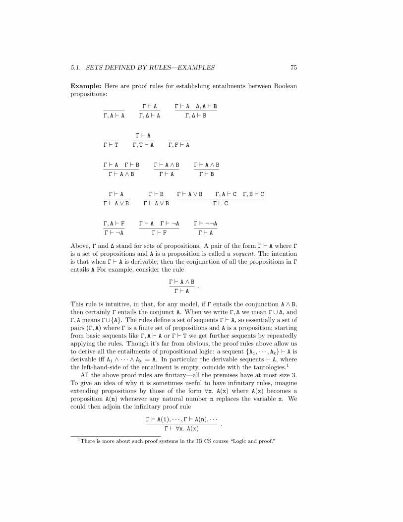
5.1. SETS DEFINED BY RULES—EXAMPLES 75
Example: Here are proof rules for establishing entailments between Booleanpropositions:
Γ, A ` AΓ ` AΓ, ∆ ` A
Γ ` A ∆, A ` BΓ, ∆ ` B
Γ ` TΓ ` AΓ, T ` A Γ, F ` A
Γ ` A Γ ` BΓ ` A ∧ B
Γ ` A ∧ BΓ ` A
Γ ` A ∧ BΓ ` B
Γ ` AΓ ` A ∨ B
Γ ` BΓ ` A ∨ B
Γ ` A ∨ B Γ, A ` C Γ, B ` CΓ ` C
Γ, A ` FΓ ` ¬A
Γ ` A Γ ` ¬AΓ ` F
Γ ` ¬¬AΓ ` A
Above, Γ and ∆ stand for sets of propositions. A pair of the form Γ ` A where Γis a set of propositions and A is a proposition is called a sequent. The intentionis that when Γ ` A is derivable, then the conjunction of all the propositions in Γentails A For example, consider the rule
Γ ` A ∧ BΓ ` A
.
This rule is intuitive, in that, for any model, if Γ entails the conjunction A ∧ B,then certainly Γ entails the conjunct A. When we write Γ, ∆ we mean Γ∪ ∆, andΓ, A means Γ∪{A}. The rules define a set of sequents Γ ` A, so essentially a set ofpairs (Γ, A) where Γ is a finite set of propositions and A is a proposition; startingfrom basic sequents like Γ, A ` A or Γ ` T we get further sequents by repeatedlyapplying the rules. Though it’s far from obvious, the proof rules above allow usto derive all the entailments of propositional logic: a sequent {A1, · · · , Ak} ` A isderivable iff A1 ∧ · · · ∧ Ak |= A. In particular the derivable sequents ` A, wherethe left-hand-side of the entailment is empty, coincide with the tautologies.1
All the above proof rules are finitary—all the premises have at most size 3.To give an idea of why it is sometimes useful to have infinitary rules, imagineextending propositions by those of the form ∀x. A(x) where A(x) becomes aproposition A(n) whenever any natural number n replaces the variable x. Wecould then adjoin the infinitary proof rule
Γ ` A(1), · · · , Γ ` A(n), · · ·Γ ` ∀x. A(x)
.
1There is more about such proof systems in the IB CS course “Logic and proof.”
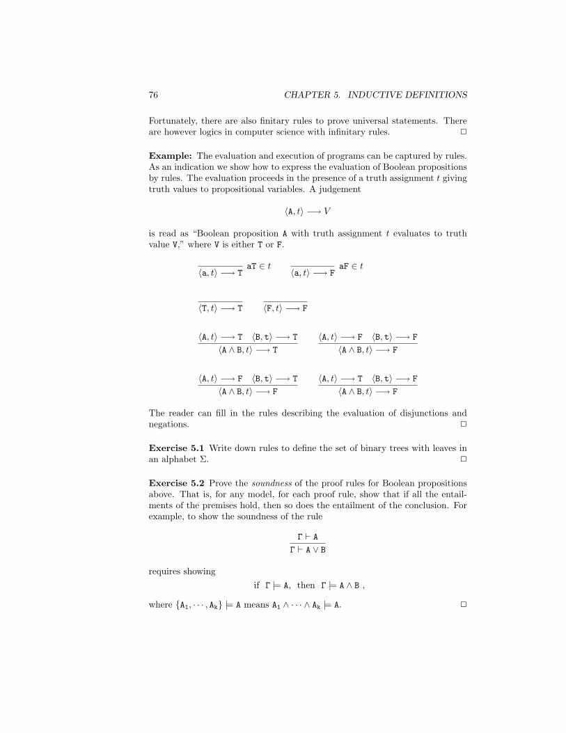
76 CHAPTER 5. INDUCTIVE DEFINITIONS
Fortunately, there are also finitary rules to prove universal statements. Thereare however logics in computer science with infinitary rules. 2
Example: The evaluation and execution of programs can be captured by rules.As an indication we show how to express the evaluation of Boolean propositionsby rules. The evaluation proceeds in the presence of a truth assignment t givingtruth values to propositional variables. A judgement
〈A, t〉 −→ V
is read as “Boolean proposition A with truth assignment t evaluates to truthvalue V,” where V is either T or F.
〈a, t〉 −→ TaT ∈ t
〈a, t〉 −→ FaF ∈ t
〈T, t〉 −→ T 〈F, t〉 −→ F
〈A, t〉 −→ T 〈B, t〉 −→ T
〈A ∧ B, t〉 −→ T
〈A, t〉 −→ F 〈B, t〉 −→ F
〈A ∧ B, t〉 −→ F
〈A, t〉 −→ F 〈B, t〉 −→ T
〈A ∧ B, t〉 −→ F
〈A, t〉 −→ T 〈B, t〉 −→ F
〈A ∧ B, t〉 −→ F
The reader can fill in the rules describing the evaluation of disjunctions andnegations. 2
Exercise 5.1 Write down rules to define the set of binary trees with leaves inan alphabet Σ. 2
Exercise 5.2 Prove the soundness of the proof rules for Boolean propositionsabove. That is, for any model, for each proof rule, show that if all the entail-ments of the premises hold, then so does the entailment of the conclusion. Forexample, to show the soundness of the rule
Γ ` AΓ ` A ∨ B
requires showingif Γ |= A, then Γ |= A ∧ B ,
where {A1, · · · , Ak} |= A means A1 ∧ · · · ∧ Ak |= A. 2
5.2. INDUCTIVELY-DEFINED SETS 77
5.2 Inductively-defined sets
We are interested in the general problem of defining a set by rules of the kindwe have seen in the examples.
In essence, an instance of a rule has the form of a pair (X/y) consisting of aset X, the premises, and a conclusion y. In general X might be empty or eveninfinite. When there is rule of the form (∅/y) we will call y an axiom. We say arule (X/y) is finitary when the set X is finite; then the rule will be of the form({x1, . . . , xn}/y), possibly with empty premises.
All examples of the previous section are associated with their own set of ruleinstances. For example, for strings Σ∗ the rule instances form the set
{(∅/ε)} ∪ {({x}/ax) | x ∈ Σ∗ & a ∈ Σ} ,
consisting of all instantiations of the rules used in building up strings. We gavetwo forms of rules for generating the nonnegative integers N0. For the first theset of rule instances is
{(∅/0)} ∪ {({n}/n+ 1) | n ∈ N0} ,
while for the second the set is
{({0, · · · , (n− 1)}/n) | n ∈ N0} .
A set of rule instances R specifies a way to build a set. A particular ruleinstance (X/y) is intended to say that if all the elements of X are in the setthen so is y. We look for the least set with this property. If it exists this shouldbe the set inductively defined by the rules.
Suppose we are given a set of rule instances R. We say a set Q is closedunder the rule instances R, or simply R-closed, iff for all rule instances (X/y)
X ⊆ Q⇒ y ∈ Q .
In other words, a set is closed under the rule instances if whenever the premisesof any rule instance lie in the set so does its conclusion. In particular, anR-closed set must contain all the axioms.
Assume a set of rule instances R. Consider the collection of all R-closedsets:
{Q | Q is R-closed} .This collection is nonempty as, for example, the set
{y | ∃X. (X/y) ∈ R}
is clearly R-closed. Thus we can form its intersection
IR =⋂{Q | Q is R-closed} .
The important fact is that IR is itself R-closed. To see this argue as follows:Let (X/y) ∈ R. Suppose X ⊆ IR. Let Q be any R-closed subset. Then X ⊆ Qand consequently y ∈ Q, as Q is R-closed. Hence y ∈ IR.
Summarising what we have just shown:
78 CHAPTER 5. INDUCTIVE DEFINITIONS
Proposition 5.3 With respect to a set of rule instances R,(i) IR is R-closed, and(ii) if Q is an R-closed set then IR ⊆ Q.
The set IR is often described as the set inductively defined by R. Proposi-tion 5.3 will supply us with a very useful proof principle for showing a prop-erty holds of all the elements of IR. The earlier examples give an idea of howwidespread inductively-defined sets are.
5.3 Rule induction
Suppose we wish to show a property P (x) is true of all elements x ∈ IR, the setinductively-defined by a set of rule instances R. The conditions (i) and (ii) inProposition 5.3 above furnish a method. Define the set
Q = {x ∈ IR | P (x)} .
The property P (x) is true of all x ∈ IR iff IR ⊆ Q. By condition (ii), to showIR ⊆ Q it suffices to show that Q is R-closed. This requires that for all ruleinstances (X/y) that
(∀x ∈ X. x ∈ IR & P (x))⇒ (y ∈ IR & P (y)) .
But IR is R-closed by (i), so this will follow precisely when
(∀x ∈ X. x ∈ IR & P (x))⇒ P (y) .
We have obtained an important, general proof principle.
The principle of rule inductionLet IR be inductively-defined by R. Then ∀x ∈ IR. P (x) if for all rule instances(X/y) in R,
(∀x ∈ X. x ∈ IR & P (x))⇒ P (y) .
(The property P (x) is called the induction hypothesis.)
[In other words to prove ∀x ∈ IR. P (x) it suffices to show that ∀x ∈ X. P (x)implies P (y) only for all rule instances (X/y) with X ⊆ IR.]
Notice for rule instances of the form (X/y), with X = ∅, the condition in thestatement of rule induction is equivalent to P (y). Certainly then ∀x ∈ X. x ∈IR & P (x) is vacuously true because any x in ∅ satisfies P (x)—there are none.
Supposing the rule instances R are finitary, the statement of rule inductionamounts to the following. For rule instances R, we have ∀y ∈ IR. P (y) iff forall axioms
y
5.3. RULE INDUCTION 79
P (y) is true, and for all rule instances
x1, . . . , xn
y
if xk ∈ IR & P (xk) is true for all the premises, when k ranges from 1 to n, thenP (y) is true of the conclusion.
The principle of rule induction is very useful to show a property is true ofall the elements in an inductively-defined set. It has many well-known instances.
Examples: Refer to the examples of rules beginning this chapter.
Nonnegative integers N0: The rules (∅/0) and ({n}/(n + 1)), for a numbern, yield mathematical induction as a special case of rule induction.
The alternative rules (∅/0) and ({0, 1, · · · , (n− 1)}/n), for a number n, yieldcourse-of-values induction, the principle that says: A property P (n) holds forall nonnegative numbers n iff for all n ∈ N0
(∀m < n. P (m))⇒ P (n) .
Notice what happens when n = 0. Then there are no m ∈ N0 with m < 0, sothe condition of the implication is vacuously true and the implication amountsto P (0). You’ll recall, course-of-values induction is useful when truth of a prop-erty at n can depend on its truth at earlier values other than just its immediatepredecessor.
Strings Σ∗: With the rules for strings over an alphabet Σ rule induction spe-cialises to this principle: a property P (x) holds of all strings x ∈ Σ∗ iff
P (ε) and∀a ∈ Σ, x ∈ Σ∗. P (x)⇒ P (ax) .
(Essentially the same induction principle works for lists.)
Boolean propositions: With the rules for the syntax of Boolean propositions,rule induction specialises to structural induction.
Proof rules for Boolean propositions: Consider now R to be the the proofrules for entailment between Boolean propositions. Rule induction yields anintuitive way to establish properties of all derivable judgments. To show aproperty holds of all derivable judgments Γ ` A it suffices to show the propertyis preserved in going from the premises to the conclusions of all the rules. WithExercise 5.2 in hand it follows that for any derivable sequent Γ ` A we have thatΓ |= A.
Evaluation of Boolean propositions: That evaluation can be captured byrules enables the use of rule induction in proving facts about the evaluation
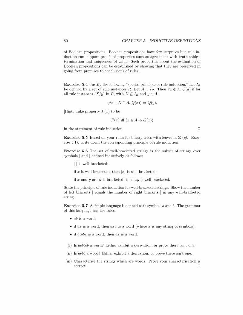
80 CHAPTER 5. INDUCTIVE DEFINITIONS
of Boolean propositions. Boolean propositions have few surprises but rule in-duction can support proofs of properties such as agreement with truth tables,termination and uniqueness of value. Such properties about the evaluation ofBoolean propositions can be established by showing that they are preserved ingoing from premises to conclusions of rules.
Exercise 5.4 Justify the following “special principle of rule induction.” Let IRbe defined by a set of rule instances R. Let A ⊆ IR. Then ∀a ∈ A. Q(a) if forall rule instances (X/y) in R, with X ⊆ IR and y ∈ A,
(∀x ∈ X ∩A. Q(x))⇒ Q(y).
[Hint: Take property P (x) to be
P (x) iff (x ∈ A⇒ Q(x))
in the statement of rule induction.] 2
Exercise 5.5 Based on your rules for binary trees with leaves in Σ (cf. Exer-cise 5.1), write down the corresponding principle of rule induction. 2
Exercise 5.6 The set of well-bracketed strings is the subset of strings oversymbols [ and ] defined inductively as follows:
[ ] is well-bracketed;
if x is well-bracketed, then [x] is well-bracketed;
if x and y are well-bracketed, then xy is well-bracketed.
State the principle of rule induction for well-bracketed strings. Show the numberof left brackets [ equals the number of right brackets ] in any well-bracketedstring. 2
Exercise 5.7 A simple language is defined with symbols a and b. The grammarof this language has the rules:
• ab is a word;
• if ax is a word, then axx is a word (where x is any string of symbols);
• if abbbx is a word, then ax is a word.
(i) Is abbbbb a word? Either exhibit a derivation, or prove there isn’t one.
(ii) Is abbb a word? Either exhibit a derivation, or prove there isn’t one.
(iii) Characterise the strings which are words. Prove your characterisation iscorrect. 2

5.3. RULE INDUCTION 81
Exercise 5.8 The set S is defined to be the least subset of natural numbers Nsuch that:
1 ∈ S;
if n ∈ S, then 3n ∈ S;
if n ∈ S and n > 2, then (n− 2) ∈ S.
Show that S = {m ∈ N | ∃r, s ∈ N∪ {0}. m = 3r − 2s}. Deduce that S is theset of odd numbers. 2
Exercise 5.9 Let I be a nonempty subset of the natural numbers N = {1, 2, 3, · · ·}.The set S is defined to be least subset of N such that
I ⊆ S, andif m,n ∈ S and m < n, then (n−m) ∈ S.
Define h to be the least member of S. This question guides you through toa proof that h coincides with the highest common factor of I, written hcf (I ),and defined to be the natural number with the properties that
hcf (I) divides n for every element n ∈ I, andif k is a natural number which divides n for every n ∈ I, then kdivides hcf (I).
(a) The set S may also be described as the least subset of N closed undercertain rules. Describe the rules. Write down a principle of rule inductionappropriate for the set S.
(b) Show by rule induction that hcf (I ) divides n for every n ∈ S.
(c) Let n ∈ S. Establish that
if p.h < n then (n− p.h) ∈ S
for all nonnegative integers p.
(d) Show that h divides n for every n ∈ S. [Hint: suppose otherwise andderive a contradiction.]
(e) Why do the results of (b) and (d) imply that h = hcf (I).
2
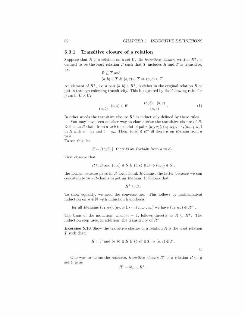
82 CHAPTER 5. INDUCTIVE DEFINITIONS
5.3.1 Transitive closure of a relation
Suppose that R is a relation on a set U . Its transitive closure, written R+, isdefined to be the least relation T such that T includes R and T is transitive,i.e.
R ⊆ T and(a, b) ∈ T & (b, c) ∈ T ⇒ (a, c) ∈ T .
An element of R+, i.e. a pair (a, b) ∈ R+, is either in the original relation R orput in through enforcing transitivity. This is captured by the following rules forpairs in U × U :
(a, b)(a, b) ∈ R (a, b) (b, c)
(a, c). (1)
In other words the transitive closure R+ is inductively defined by these rules.You may have seen another way to characterise the transitive closure of R.
Define an R-chain from a to b to consist of pairs (a1, a2), (a2, a3), · · · , (an−1, an)in R with a = a1 and b = an. Then, (a, b) ∈ R+ iff there is an R-chain from ato b.To see this, let
S = {(a, b) | there is an R-chain from a to b} .
First observe that
R ⊆ S and (a, b) ∈ S & (b, c) ∈ S ⇒ (a, c) ∈ S ,
the former because pairs in R form 1-link R-chains, the latter because we canconcatenate two R-chains to get an R-chain. It follows that
R+ ⊆ S .
To show equality, we need the converse too. This follows by mathematicalinduction on n ∈ N with induction hypothesis:
for all R-chains (a1, a2), (a2, a3), · · · , (an−1, an) we have (a1, an) ∈ R+ .
The basis of the induction, when n = 1, follows directly as R ⊆ R+. Theinduction step uses, in addition, the transitivity of R+.
Exercise 5.10 Show the transitive closure of a relation R is the least relationT such that:
R ⊆ T and (a, b) ∈ R & (b, c) ∈ T ⇒ (a, c) ∈ T .
2
One way to define the reflexive, transitive closure R∗ of a relation R on aset U is as
R∗ = idU ∪R+ .
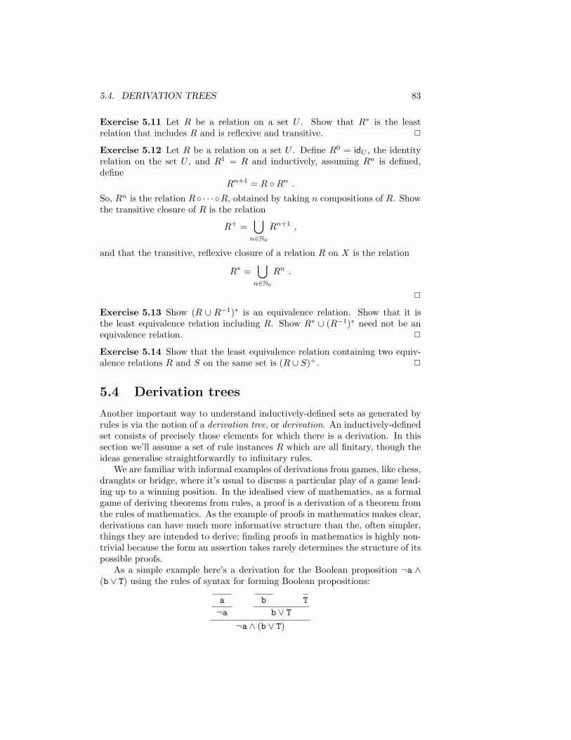
5.4. DERIVATION TREES 83
Exercise 5.11 Let R be a relation on a set U . Show that R∗ is the leastrelation that includes R and is reflexive and transitive. 2
Exercise 5.12 Let R be a relation on a set U . Define R0 = idU , the identityrelation on the set U , and R1 = R and inductively, assuming Rn is defined,define
Rn+1 = R ◦Rn .So, Rn is the relation R◦ · · · ◦R, obtained by taking n compositions of R. Showthe transitive closure of R is the relation
R+ =⋃n∈N0
Rn+1 ,
and that the transitive, reflexive closure of a relation R on X is the relation
R∗ =⋃n∈N0
Rn .
2
Exercise 5.13 Show (R ∪ R−1)∗ is an equivalence relation. Show that it isthe least equivalence relation including R. Show R∗ ∪ (R−1)∗ need not be anequivalence relation. 2
Exercise 5.14 Show that the least equivalence relation containing two equiv-alence relations R and S on the same set is (R ∪ S)+. 2
5.4 Derivation trees
Another important way to understand inductively-defined sets as generated byrules is via the notion of a derivation tree, or derivation. An inductively-definedset consists of precisely those elements for which there is a derivation. In thissection we’ll assume a set of rule instances R which are all finitary, though theideas generalise straightforwardly to infinitary rules.
We are familiar with informal examples of derivations from games, like chess,draughts or bridge, where it’s usual to discuss a particular play of a game lead-ing up to a winning position. In the idealised view of mathematics, as a formalgame of deriving theorems from rules, a proof is a derivation of a theorem fromthe rules of mathematics. As the example of proofs in mathematics makes clear,derivations can have much more informative structure than the, often simpler,things they are intended to derive; finding proofs in mathematics is highly non-trivial because the form an assertion takes rarely determines the structure of itspossible proofs.
As a simple example here’s a derivation for the Boolean proposition ¬a ∧(b ∨ T) using the rules of syntax for forming Boolean propositions:
a
¬ab T
b ∨ T¬a ∧ (b ∨ T)
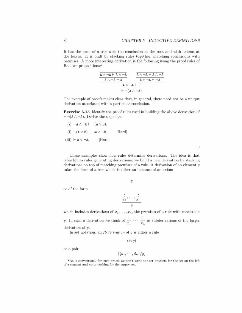
84 CHAPTER 5. INDUCTIVE DEFINITIONS
It has the form of a tree with the conclusion at the root and with axioms atthe leaves. It is built by stacking rules together, matching conclusions withpremises. A more interesting derivation is the following using the proof rules ofBoolean propositions:2
A ∧ ¬A ` A ∧ ¬AA ∧ ¬A ` A
A ∧ ¬A ` A ∧ ¬AA ∧ ¬A ` ¬A
A ∧ ¬A ` F` ¬(A ∧ ¬A)
The example of proofs makes clear that, in general, there need not be a uniquederivation associated with a particular conclusion.
Exercise 5.15 Identify the proof rules used in building the above derivation of` ¬(A ∧ ¬A). Derive the sequents:
(i) ¬A ∧ ¬B ` ¬(A ∨ B),
(i) ¬(A ∨ B) ` ¬A ∧ ¬B, [Hard]
(iii) ` A ∨ ¬A. [Hard]
2
These examples show how rules determine derivations. The idea is thatrules lift to rules generating derivations; we build a new derivation by stackingderivations on top of matching premises of a rule. A derivation of an element ytakes the form of a tree which is either an instance of an axiom
y
or of the form...x1, . . . ,
...xn
y
which includes derivations of x1, . . . , xn, the premises of a rule with conclusion
y. In such a derivation we think of...x1, · · · ,
...xn
as subderivations of the larger
derivation of y.In set notation, an R-derivation of y is either a rule
(∅/y)
or a pair({d1, · · · , dn}/y)
2As is conventional for such proofs we don’t write the set brackets for the set on the leftof a sequent and write nothing for the empty set.
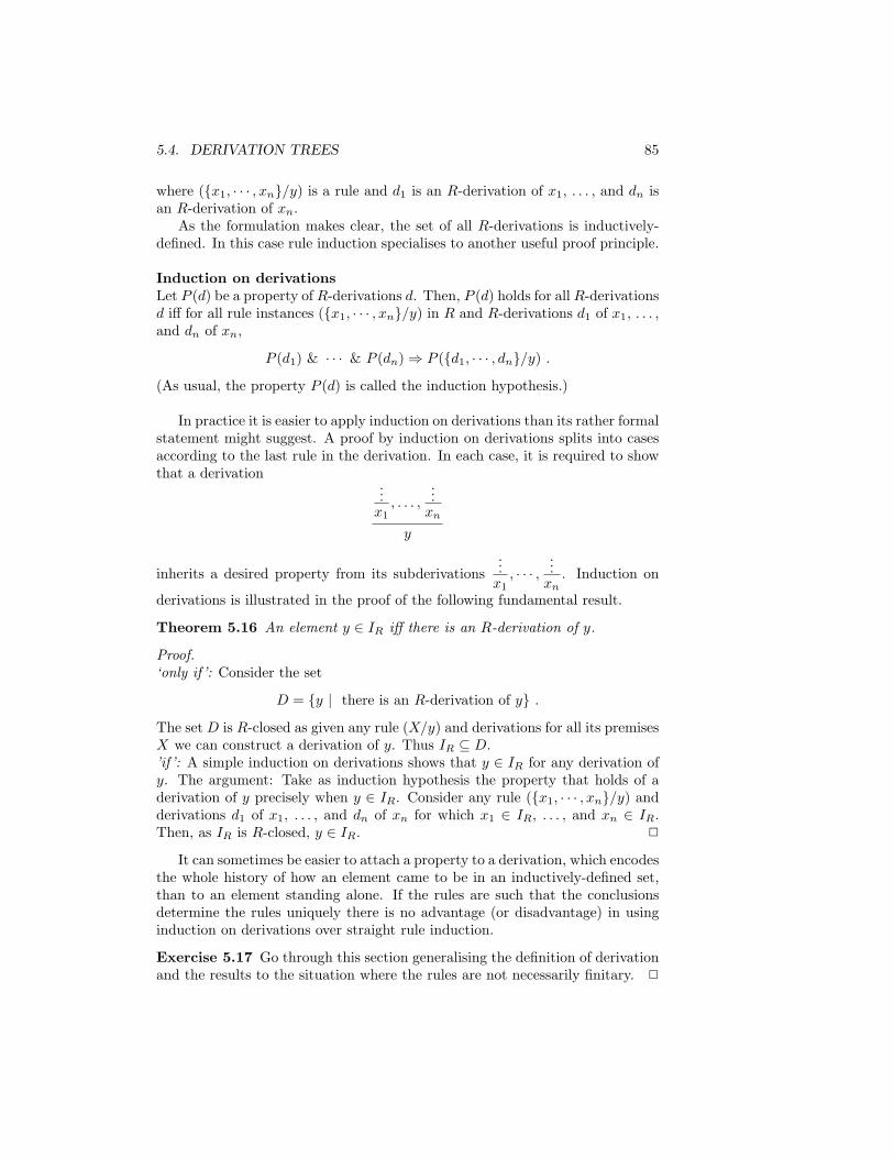
5.4. DERIVATION TREES 85
where ({x1, · · · , xn}/y) is a rule and d1 is an R-derivation of x1, . . . , and dn isan R-derivation of xn.
As the formulation makes clear, the set of all R-derivations is inductively-defined. In this case rule induction specialises to another useful proof principle.
Induction on derivationsLet P (d) be a property of R-derivations d. Then, P (d) holds for all R-derivationsd iff for all rule instances ({x1, · · · , xn}/y) in R and R-derivations d1 of x1, . . . ,and dn of xn,
P (d1) & · · · & P (dn)⇒ P ({d1, · · · , dn}/y) .
(As usual, the property P (d) is called the induction hypothesis.)
In practice it is easier to apply induction on derivations than its rather formalstatement might suggest. A proof by induction on derivations splits into casesaccording to the last rule in the derivation. In each case, it is required to showthat a derivation
...x1, . . . ,
...xn
y
inherits a desired property from its subderivations...x1, · · · ,
...xn
. Induction on
derivations is illustrated in the proof of the following fundamental result.
Theorem 5.16 An element y ∈ IR iff there is an R-derivation of y.
Proof.‘only if ’: Consider the set
D = {y | there is an R-derivation of y} .
The set D is R-closed as given any rule (X/y) and derivations for all its premisesX we can construct a derivation of y. Thus IR ⊆ D.’if ’: A simple induction on derivations shows that y ∈ IR for any derivation ofy. The argument: Take as induction hypothesis the property that holds of aderivation of y precisely when y ∈ IR. Consider any rule ({x1, · · · , xn}/y) andderivations d1 of x1, . . . , and dn of xn for which x1 ∈ IR, . . . , and xn ∈ IR.Then, as IR is R-closed, y ∈ IR. 2
It can sometimes be easier to attach a property to a derivation, which encodesthe whole history of how an element came to be in an inductively-defined set,than to an element standing alone. If the rules are such that the conclusionsdetermine the rules uniquely there is no advantage (or disadvantage) in usinginduction on derivations over straight rule induction.
Exercise 5.17 Go through this section generalising the definition of derivationand the results to the situation where the rules are not necessarily finitary. 2
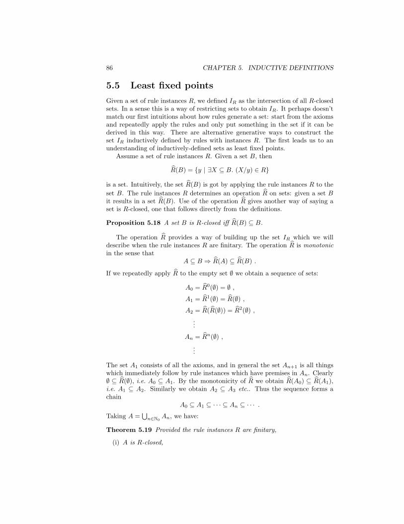
86 CHAPTER 5. INDUCTIVE DEFINITIONS
5.5 Least fixed points
Given a set of rule instances R, we defined IR as the intersection of all R-closedsets. In a sense this is a way of restricting sets to obtain IR. It perhaps doesn’tmatch our first intuitions about how rules generate a set: start from the axiomsand repeatedly apply the rules and only put something in the set if it can bederived in this way. There are alternative generative ways to construct theset IR inductively defined by rules with instances R. The first leads us to anunderstanding of inductively-defined sets as least fixed points.
Assume a set of rule instances R. Given a set B, then
R(B) = {y | ∃X ⊆ B. (X/y) ∈ R}
is a set. Intuitively, the set R(B) is got by applying the rule instances R to theset B. The rule instances R determines an operation R on sets: given a set Bit results in a set R(B). Use of the operation R gives another way of saying aset is R-closed, one that follows directly from the definitions.
Proposition 5.18 A set B is R-closed iff R(B) ⊆ B.
The operation R provides a way of building up the set IR which we willdescribe when the rule instances R are finitary. The operation R is monotonicin the sense that
A ⊆ B ⇒ R(A) ⊆ R(B) .
If we repeatedly apply R to the empty set ∅ we obtain a sequence of sets:
A0 = R0(∅) = ∅ ,
A1 = R1(∅) = R(∅) ,
A2 = R(R(∅)) = R2(∅) ,...
An = Rn(∅) ,...
The set A1 consists of all the axioms, and in general the set An+1 is all thingswhich immediately follow by rule instances which have premises in An. Clearly∅ ⊆ R(∅), i.e. A0 ⊆ A1. By the monotonicity of R we obtain R(A0) ⊆ R(A1),i.e. A1 ⊆ A2. Similarly we obtain A2 ⊆ A3 etc.. Thus the sequence forms achain
A0 ⊆ A1 ⊆ · · · ⊆ An ⊆ · · · .
Taking A =⋃n∈N0
An, we have:
Theorem 5.19 Provided the rule instances R are finitary,
(i) A is R-closed,
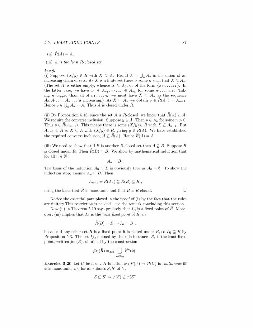
5.5. LEAST FIXED POINTS 87
(ii) R(A) = A,
(iii) A is the least R-closed set.
Proof.(i) Suppose (X/y) ∈ R with X ⊆ A. Recall A =
⋃nAn is the union of an
increasing chain of sets. As X is a finite set there is some n such that X ⊆ An.(The set X is either empty, whence X ⊆ A0, or of the form {x1, . . . , xk}. Inthe latter case, we have x1 ∈ An1 , · · · , xk ∈ Ank for some n1, . . . , nk. Tak-ing n bigger than all of n1, . . . , nk we must have X ⊆ An as the sequenceA0, A1, . . . , An, . . . is increasing.) As X ⊆ An we obtain y ∈ R(An) = An+1.Hence y ∈
⋃nAn = A. Thus A is closed under R.
(ii) By Proposition 5.18, since the set A is R-closed, we know that R(A) ⊆ A.We require the converse inclusion. Suppose y ∈ A. Then y ∈ An for some n > 0.Thus y ∈ R(An−1). This means there is some (X/y) ∈ R with X ⊆ An−1. ButAn−1 ⊆ A so X ⊆ A with (X/y) ∈ R, giving y ∈ R(A). We have establishedthe required converse inclusion, A ⊆ R(A). Hence R(A) = A.
(iii) We need to show that if B is another R-closed set then A ⊆ B. Suppose Bis closed under R. Then R(B) ⊆ B. We show by mathematical induction thatfor all n ∈ N0
An ⊆ B .
The basis of the induction A0 ⊆ B is obviously true as A0 = ∅. To show theinduction step, assume An ⊆ B. Then
An+1 = R(An) ⊆ R(B) ⊆ B ,
using the facts that R is monotonic and that B is R-closed. 2
Notice the essential part played in the proof of (i) by the fact that the rulesare finitary.This restriction is needed—see the remark concluding this section.
Now (ii) in Theorem 5.19 says precisely that IR is a fixed point of R. More-over, (iii) implies that IR is the least fixed point of R, i.e.
R(B) = B ⇒ IR ⊆ B ,
because if any other set B is a fixed point it is closed under R, so IR ⊆ B byProposition 5.3. The set IR, defined by the rule instances R, is the least fixedpoint, written fix (R), obtained by the construction
fix (R) =def
⋃n∈N0
Rn(∅) .
Exercise 5.20 Let U be a set. A function ϕ : P(U) → P(U) is continuous iffϕ is monotonic, i.e. for all subsets S, S′ of U ,
S ⊆ S′ ⇒ ϕ(S) ⊆ ϕ(S′)
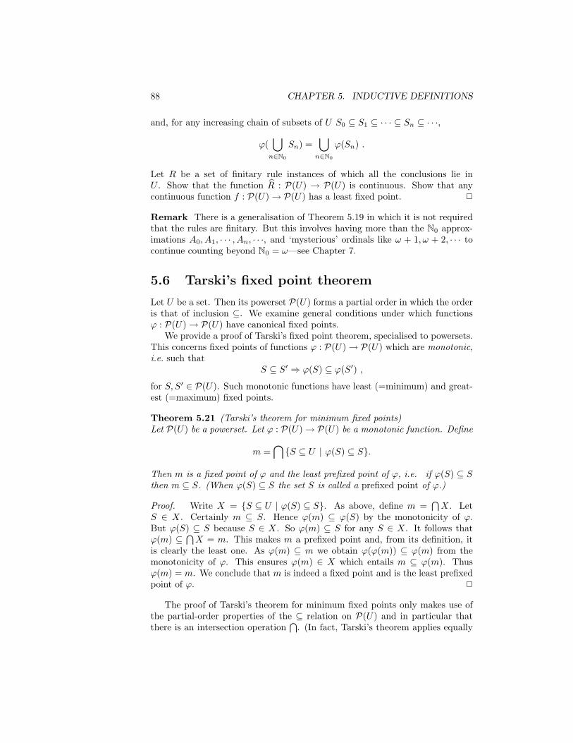
88 CHAPTER 5. INDUCTIVE DEFINITIONS
and, for any increasing chain of subsets of U S0 ⊆ S1 ⊆ · · · ⊆ Sn ⊆ · · ·,
ϕ(⋃n∈N0
Sn) =⋃n∈N0
ϕ(Sn) .
Let R be a set of finitary rule instances of which all the conclusions lie inU . Show that the function R : P(U) → P(U) is continuous. Show that anycontinuous function f : P(U)→ P(U) has a least fixed point. 2
Remark There is a generalisation of Theorem 5.19 in which it is not requiredthat the rules are finitary. But this involves having more than the N0 approx-imations A0, A1, · · · , An, · · ·, and ‘mysterious’ ordinals like ω + 1, ω + 2, · · · tocontinue counting beyond N0 = ω—see Chapter 7.
5.6 Tarski’s fixed point theorem
Let U be a set. Then its powerset P(U) forms a partial order in which the orderis that of inclusion ⊆. We examine general conditions under which functionsϕ : P(U)→ P(U) have canonical fixed points.
We provide a proof of Tarski’s fixed point theorem, specialised to powersets.This concerns fixed points of functions ϕ : P(U)→ P(U) which are monotonic,i.e. such that
S ⊆ S′ ⇒ ϕ(S) ⊆ ϕ(S′) ,
for S, S′ ∈ P(U). Such monotonic functions have least (=minimum) and great-est (=maximum) fixed points.
Theorem 5.21 (Tarski’s theorem for minimum fixed points)Let P(U) be a powerset. Let ϕ : P(U)→ P(U) be a monotonic function. Define
m =⋂{S ⊆ U | ϕ(S) ⊆ S}.
Then m is a fixed point of ϕ and the least prefixed point of ϕ, i.e. if ϕ(S) ⊆ Sthen m ⊆ S. (When ϕ(S) ⊆ S the set S is called a prefixed point of ϕ.)
Proof. Write X = {S ⊆ U | ϕ(S) ⊆ S}. As above, define m =⋂X. Let
S ∈ X. Certainly m ⊆ S. Hence ϕ(m) ⊆ ϕ(S) by the monotonicity of ϕ.But ϕ(S) ⊆ S because S ∈ X. So ϕ(m) ⊆ S for any S ∈ X. It follows thatϕ(m) ⊆
⋂X = m. This makes m a prefixed point and, from its definition, it
is clearly the least one. As ϕ(m) ⊆ m we obtain ϕ(ϕ(m)) ⊆ ϕ(m) from themonotonicity of ϕ. This ensures ϕ(m) ∈ X which entails m ⊆ ϕ(m). Thusϕ(m) = m. We conclude that m is indeed a fixed point and is the least prefixedpoint of ϕ. 2
The proof of Tarski’s theorem for minimum fixed points only makes use ofthe partial-order properties of the ⊆ relation on P(U) and in particular thatthere is an intersection operation
⋂. (In fact, Tarski’s theorem applies equally
5.6. TARSKI’S FIXED POINT THEOREM 89
well to a complete lattice with an abstract partial order and greatest lowerbound.) Replacing the roles of the order ⊆ and intersection
⋂by the converse
relation ⊇ and union⋃
we obtain a proof of the dual result for maximum fixedpoints.
Theorem 5.22 (Tarski’s theorem for maximum fixed points)Let P(U) be a powerset. Let ϕ : P(U)→ P(U) be a monotonic function. Define
M =⋃{S ⊆ U | S ⊆ ϕ(S)}.
Then M is a fixed point of ϕ and the greatest postfixed point of ϕ, i.e. ifS ⊆ ϕ(S) then S ⊆ M . (When S ⊆ ϕ(S) the set S is called a postfixed pointof ϕ.)
Notation: The minimum fixed point is traditionally written µX.ϕ(X) , and themaximum fixed point as νX.ϕ(X). Minimum and maximum fixed points arevery important in verification, in particular in model checking—the automaticverification that a process satisfies a property.
Tarski’s theorem for minimum fixed points provides another way to under-stand sets inductively defined by rules. Assuming that all the rule instancesR have conclusions in the set U , we can turn R into a monotonic functionR : P(U)→ P(U), where for S ∈ P(U)
R(S) = {y | ∃X ⊆ S. (X/y) ∈ R} .
Prefixed points of R coincide with R-closed subsets of U and the least fixedpoint of ϕR with the set IR inductively defined by the rule instances R.
Sets defined as maximum fixed points are often called coinductively definedsets.
Exercise 5.23 Supply a direct proof of Tarski’s theorem (Theorem 5.22 above)for maximum fixed points. 2
Exercise 5.24 Refer to Exercise 3.20 which defines the bisimilarity relation ∼for a directed graph (P,−→). Define
ϕ : P(P × P )→ P(P × P )
—so ϕ is a function from relations on P to relations on P—by:
p ϕ(R) q iff
• ∀p′ ∈ P. p −→ p′ ⇒ ∃q′ ∈ P. q −→ q′ & p′Rq′, and
• ∀q′ ∈ P. q −→ q′ ⇒ ∃p′ ∈ P. p −→ p′ & p′Rq′.
Show that ϕ is monotonic, has postfixed points precisely the bisimulations onP , and that the bisimilarity relation ∼ coincides with its maximum fixed point.
2
90 CHAPTER 5. INDUCTIVE DEFINITIONS
Exercise 5.25 Streams, or infinite lists, of values in a set V can be representedas functions
V∞ =def (N0 → V ) .
The head and tail of a stream L are defined by
head(L) = L(0)tail(L)(n) = L(n+ 1) for n ∈ N0 .
Define a function ϕ : P(V∞ × V∞)→ P(V∞ × V∞) by taking
L ϕ(R) M iff head(L) = head(M) and tail(L) R tail(M) .
Show that ϕ is monotonic. A stream-bisimulation is a postfixed point of ϕ,i.e. a relation R between streams such that
If L R M then head(L) = head(M) and tail(L) R tail(M) .
Show by mathematical induction that, for any stream bisimulation R,
if L R M then L = M .
Deduce that the greatest fixed point of ϕ is idV∞ . Deduce the principle ofcoinduction for streams: Streams L,M ∈ V∞ are equal if there is a stream-bisimulation relating them. 2
Exercise 5.26 Let ϕ : P(N)→ P(N) be the function given by
ϕ(U) = {3n/2 | n ∈ U & n is even} ∪ {n | n ∈ U & n is odd} .
(i) Show ϕ is monotonic with respect to ⊆.
(ii) Suppose that U ⊆ ϕ(U), i.e. U is a postfixed point of ϕ. Show that
n ∈ U & n is even⇒ 2n/3 ∈ U .
Deduce that all members of U are odd. [Hint: Assume there is an evenmember of U , so a least even member of U , to derive a contradiction.]
(iii) Deduce that the maximum fixed point of ϕ is the set of all odd numbers.
(iv) Characterise the prefixed points of ϕ. What is the minimum fixed pointof ϕ?
2
Chapter 6
Well-founded induction
This chapter introduces the powerful general proof principle of well-founded in-duction and its associated method of definition called well-founded recursion.They are based on the concept of a well-founded relation. Well-founded induc-tion has many applications but is especially important for defining and provingproperties of terminating programs.
6.1 Well-founded relations
Mathematical and structural induction are special cases of a general and power-ful proof principle called well-founded induction. In essence structural inductionworks because breaking down an expression into subexpressions cannot go onforever, eventually it must lead to atomic expressions which cannot be brokendown any further. If a property fails to hold of any expression then it must failon some minimal expression which when it is broken down yields subexpres-sions, all of which satisfy the property. This observation justifies the principleof structural induction: to show a property holds of all expressions it is suffi-cient to show that property holds of an arbitrary expression if it holds of all itssubexpressions. Similarly with the natural numbers, if a property fails to holdof all natural numbers then there has to be a smallest natural number at whichit fails. The essential feature shared by both the subexpression relation and thepredecessor relation on natural numbers is that they do not give rise to infinitedescending chains. This is the feature required of a relation if it is to supportwell-founded induction.
Definition: A well-founded relation is a binary relation ≺ on a set A such thatthere are no infinite descending chains · · · ≺ ai ≺ · · · ≺ a1 ≺ a0. When a ≺ bwe say a is a predecessor of b.
Note a well-founded relation is necessarily irreflexive i.e., for no a do wehave a ≺ a, as otherwise there would be the infinite descending chain · · · ≺ a ≺
91
92 CHAPTER 6. WELL-FOUNDED INDUCTION
· · · ≺ a ≺ a. We shall generally write � for the reflexive closure of the relation≺, i.e.
a � b ⇐⇒ a = b or a ≺ b.(A relation ≺ for which � is a total order is traditionally called a well-order.)
Sometimes one sees an alternative definition of well-founded relation, interms of minimal elements.
Proposition 6.1 Let ≺ be a binary relation on a set A. The relation ≺ iswell-founded iff any nonempty subset Q of A has a minimal element, i.e. anelement m such that
m ∈ Q & ∀b ≺ m. b /∈ Q.
Proof.“if”: Suppose every nonempty subset of A has a minimal element. If · · · ≺ ai ≺· · · ≺ a1 ≺ a0 were an infinite descending chain then the set Q = {ai | i ∈ N0}would be nonempty without a minimal element, a contradiction. Hence ≺ iswell-founded.“only if”: To see this, suppose Q is a nonempty subset of A. Construct achain of elements as follows. Take a0 to be any element of Q. Inductively,assume a chain of elements an ≺ · · · ≺ a0 has been constructed inside Q. Eitherthere is some b ≺ an such that b ∈ Q or there is not. If not , then stopthe construction. Otherwise take an+1 = b. As ≺ is well-founded the chain· · · ≺ ai ≺ · · · ≺ a1 ≺ a0 cannot be infinite. Hence it is finite, of the forman ≺ · · · ≺ a0 with ∀b ≺ an. b /∈ Q. Take the required minimal element m to bean. 2
Exercise 6.2 Let ≺ be a well-founded relation on a set B. Prove
(i) its transitive closure ≺+ is also well-founded,
(ii) its reflexive, transitive closure ≺∗ is a partial order.
2
6.2 Well-founded induction
Well-founded relations support an important proof principle.
The principle of well-founded inductionLet ≺ be a well founded relation on a set A. To show ∀a ∈ A. P (a) it sufficesto prove that for all a ∈ A
[∀b ≺ a. P (b)]⇒ P (a) .
The principle reduces showing that a property (the induction hypothesis) holdsglobally to showing that the property is preserved locally by the well foundedrelation.
6.2. WELL-FOUNDED INDUCTION 93
We now prove the principle. The proof rests on the observation, Proposi-tion 6.1, that any nonempty subset Q of a set A with a well-founded relation≺ has a minimal element. To justify the principle, we assume ∀a ∈ A. ([∀b ≺a. P (b)] ⇒ P (a)) and produce a contradiction by supposing ¬P (a) for somea ∈ A. Then, as we have observed, there must be a minimal element m of theset {a ∈ A | ¬P (a)}. But then ¬P (m) and yet ∀b ≺ m. P (b), which contradictsthe assumption.
Example: If we take the relation ≺ to be the predecessor relation
n ≺ m iff m = n+ 1
on the non-negative integers the principle of well-founded induction specialisesto mathematical induction. 2
Example: If we take ≺ to be the “strictly less than” relation < on the non-negative integers, the principle specialises to course-of-values induction: To showP (n) for all nonnegative integers n, it suffices to show
(∀m < n. P (m))⇒ P (n)
for all nonnegative integers n. 2
Example: If we take ≺ to be the relation between expressions such that a ≺b holds iff a is an immediate subexpression of b we obtain the principle ofstructural induction as a special case of well-founded induction. 2
Proposition 6.1 provides an alternative to proofs by the principle of well-founded induction. Suppose A is a well-founded set. Instead of using well-founded induction to show every element of A satisfies a property, we can con-sider the subset of A for which the property fails, i.e. the subset Q of coun-terexamples. By Proposition 6.1, to show Q is ∅ it is sufficient to show thatQ cannot have a minimal element. This is done by obtaining a contradictionfrom the assumption that there is a minimal element in Q. Whether to use thisapproach or the principle of well-founded induction is largely a matter of taste,though sometimes, depending on the problem, one approach can be more directthan the other.
A special instance of Proposition 6.1 is well-known to be equivalent to math-ematical induction. It is the principle that every nonempty subset of naturalnumbers has a least element.
Exercise 6.3 For a suitable well-founded relation on strings, use the “no coun-terexample” approach described above to show there is no string u which satisfiesau = ub for two distinct symbols a and b. 2
Well-founded induction is the most important principle in proving the ter-mination of programs. Uncertainties about termination arise because of loopsor recursions in a program. If it can be shown that execution of a loop or re-cursion in a program decreases the value in a well-founded set then executionmust eventually terminate.
94 CHAPTER 6. WELL-FOUNDED INDUCTION
6.3 Building well-founded relations
Applying the principle of well-founded induction often depends on a judiciouschoice of well-founded relation.
6.3.1 Fundamental well-founded relations
We have already made use of well-founded relations like that of proper subex-pression on syntactic sets, or < on natural numbers. More generally, in Sec-tion 5.4 we saw that any set inductively-defined by rule instances R was asso-ciated with a set of R-derivations. The subderivation relation is a well-foundedrelation on R-derivations—see Exercise 6.4 below. In many cases each elementof an inductively-defined set IR has a unique derivation (e.g. the case for N0 andsimple syntax, such as that of Boolean propositions). Then the well-foundedrelation on R-derivations transfers directly to a well-founded relation on IR.
Exercise 6.4 Let R be a collection of finitary rule instances. For R-derivationsd, d′ define
d′ ≺ d iff ∃D, y. d = (D/y) & d′ ∈ D .
By using induction on derivations with a suitable induction hypothesis, show ≺is well-founded. 2
Here are some ways to construct further well-founded relations. Recall thatwe use x � y to mean (x ≺ y or x = y).
6.3.2 Transitive closure
If ≺ is well-founded relation on A, then so is its transitive closure ≺+. Clearlyany infinite descending chain
· · · ≺+ an ≺+ · · · ≺+ a1 ≺+ a0
with respect to ≺+ would induce an infinite descending chain with respect to≺. (This was part of an earlier exercise!)
6.3.3 Product
If ≺1 is well-founded on A1 and ≺2 is well-founded on A2 then taking
(a1, a2) � (a′1, a′2)⇔def a1 �1 a
′1 and a2 �2 a
′2
determines a relation ≺= (� \idA1×A2) in A1 ×A2 called the product relation:
Proposition 6.5 The product relation of well-founded relations is well-founded.
6.3. BUILDING WELL-FOUNDED RELATIONS 95
Proof. Suppose ≺1 is well-founded on A1 and ≺2 is well-founded on A2.Assume their product relation ≺ is not well-founded, i.e. that there is an infinitedescending chain
· · · ≺ (xn, yn) ≺ · · · ≺ (x1, y1) ≺ (x0, y0) .
But then, from the definition of the product relation ≺, either
· · · ≺1 xnk ≺1 · · · ≺1 xn1 ≺1 xn0
or· · · ≺2 ynk ≺2 · · · ≺2 yn1 ≺2 yn0 ,
which contradicts the well-foundedness of ≺1 and ≺2. 2
We’ll see applications of the product of well-founded relations in the nextsection. However product relations are not as generally applicable as thoseproduced by lexicographic products.
6.3.4 Lexicographic products
Let ≺1 be well-founded on A1 and ≺2 be well-founded on A2. Define theirlexicographic product by
(a1, a2) ≺lex (a′1, a′2) iff a1 ≺1 a
′1 or (a1 = a′1 & a2 ≺2 a
′2) .
Proposition 6.6 The lexicographic product of well-founded relations is well-founded.
Proof. Suppose ≺1 is well-founded on A1 and ≺2 is well-founded on A2.Assume their lexicographic product ≺lex is not well-founded, i.e. that there isan infinite descending chain
· · · ≺ (xn, yn) ≺ · · · ≺ (x1, y1) ≺ (x0, y0) .
From the definition of the lexicographic relation ≺lex· · · �1 xn �1 · · · �1 x1 �1 x0 .
But ≺1 is well-founded so from some stage on, say m ≥ n, this chain is constant.But then from the definition of the lexicographic relation ≺,
· · · ≺2 yn+i ≺2 · · · ≺2 yn+1 ≺2 yn ,
which contradicts the well-foundedness of ≺2. 2
Exercise 6.7 Let ≺ be a well-founded relation on a set X such that � is atotal order. Show it need not necessarily make the set
{x ∈ X | x ≺ y}
finite for all y ∈ X.[Recall a total order is a partial order ≤ such that x ≤ y or y ≤ x for all itselements x, y. Hint: Consider the lexicographic product of < and < on N0×N0.]
2
96 CHAPTER 6. WELL-FOUNDED INDUCTION
6.3.5 Inverse image
Let f : A→ B be a function and ≺B a well-founded relation on B. Then ≺A iswell-founded on A where
a ≺A a′ ⇔def f(a) ≺B f(a′)
for a, a′ ∈ A.
Exercise 6.8 Show the inverse image of a well-founded relation is a well-founded relation. 2
6.4 Applications
6.4.1 Euclid’s algorithm for hcf
We can use well-founded induction to show the correctness of Euclid’s algorithmfor calculating the highest common factor (hcf) of a pair of natural numbers.1
One way to formulate Euclid’s algorithm is through a reduction relation −→E
on N× N defined as follows:
(m,n) −→E (m,n−m) if m < n ,
(m,n) −→E (m− n, n) if n < m .
So (m,n) reduces to (m,n −m) if m < n and to (m − n, n) if n < m. Noticethere is no reduction when m = n; in this case the reduction terminates.
It is easy to check that the following properties hold for the hcf of naturalnumbers:
Proposition 6.9
(a) hcf(m,n) = hcf(m,n−m) if m < n,
(b) hcf(m,n) = hcf(m− n, n) if n < m,
(c) hcf(m,m) = m.
Proof. The highest common factor of natural numbers m and n, hcf(m,n), ischaracterised by:
(i) hcf(m,n) divides m and n;
(ii) if k divides m and n, then k divides hcf(m,n).
1Another name for highest common factor is greatest common divisor (gcd).
6.4. APPLICATIONS 97
In all cases the proof proceeds by showing any divisor of the left is also a divisorof the right and vice versa; two natural numbers with the same divisors mustbe equal. As an example we show (a) hcf(m,n) = hcf(m,n − m) assumingm < n. Suppose k divides the lhs hcf(m,n). Then k certainly divides m andn by (i), and so divides m and n −m. Thus k divides the rhs hcf(m,n −m)by (ii). Suppose now that k divides the rhs hcf(m,n −m). Then k divides mand n −m by (i). It follows that k divides m and n, and so the lhs hcf(m,n)by (ii). 2
Euclid’s reduction terminates with the hcf of the natural numbers it startswith:
Theorem 6.10 For all m,n ∈ N,
(m,n) −→∗E (hcf(m,n), hcf(m,n)) .
Proof. Let ≺⊆ N× N be the well-founded relation constructed as the productof < and < on N. Take
P (m,n)⇔def (m,n) −→∗E (hcf(m,n), hcf(m,n))
as the induction hypothesis. We prove P (m,n) for all m,n ∈ N by well-foundedinduction.
Let (m,n) ∈ N × N. Assume P (m′, n′) for all (m′, n′) ≺ (m,n). Considerthe cases:
Case m < n. In this case (m,n) −→E (m,n−m) and because P (m,n−m) bythe induction hypothesis,
(m,n−m) −→∗E (hcf(m,n−m), hcf(m,n−m)) .
Hence(m,n) −→∗E (hcf(m,n−m), hcf(m,n−m)) ,
by the properties of the reflexive transitive closure −→∗E . Also hcf(m,n) =hcf(m,n−m). Thus P (m,n) in this case.
Case n < m. This case is very similar.
Case m = n. In this case(m,n) −→∗E (m,n)
as −→∗E is reflexive. Also hcf(m,n) = m = n. Thus P (m,n) in this case.
In all possible cases for (m,n) we can derive P (m,n) from the assumptionthat P (m′, n′) holds for all ≺-predecessors (m′, n′). Hence by well-foundedinduction we have established P (m,n) for all m,n ∈ N. 2
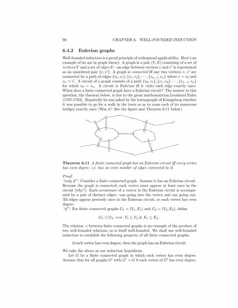
98 CHAPTER 6. WELL-FOUNDED INDUCTION
6.4.2 Eulerian graphs
Well-founded induction is a proof principle of widespread applicability. Here’s anexample of its use in graph theory. A graph is a pair (V,E) consisting of a set ofvertices V and a set of edges E—an edge between vertices v and v′ is representedas an unordered pair {v, v′}. A graph is connected iff any two vertices v, v′ areconnected by a path of edges {v0, v1}, {v1, v2}, · · · , {vn−1, vn} where v = v0 andvn = v′. A circuit of a graph consists of a path {v0, v1}, {v1, v2}, · · · , {vn−1, vn}for which v0 = vn. A circuit is Eulerian iff it visits each edge exactly once.When does a finite connected graph have a Eulerian circuit? The answer to thisquestion, the theorem below, is due to the great mathematician Leonhard Euler(1707-1783). Reputedly he was asked by the townspeople of Konigsberg whetherit was possible to go for a walk in the town so as to cross each of its numerousbridges exactly once (Was it? See the figure and Theorem 6.11 below).
HH """(((
((XXXXPPPPPPP((((��
����hhQQ
��(((lll
����hhHH
EE((((c
cc
((((XXXXXXXXXXX������
������
AAA
AAA
���
���
����
����
BBBB
BBBB
Theorem 6.11 A finite connected graph has an Eulerian circuit iff every vertexhas even degree, i.e. has an even number of edges connected to it.
Proof.“only if”: Consider a finite connected graph. Assume it has an Eulerian circuit.Because the graph is connected, each vertex must appear at least once in thecircuit (why?). Each occurrence of a vertex in the Eulerian circuit is accompa-nied by a pair of distinct edges—one going into the vertex and one going out.All edges appear precisely once in the Eulerian circuit, so each vertex has evendegree.“if”: For finite connected graphs G1 = (V1, E1) and G2 = (V2, E2), define
G1 � G2 ⇐⇒ V1 ⊆ V2 & E1 ⊆ E2 .
The relation ≺ between finite connected graphs is an example of the product oftwo well-founded relations, so is itself well-founded. We shall use well-foundedinduction to establish the following property of all finite connected graphs:
if each vertex has even degree, then the graph has an Eulerian circuit.
We take the above as our induction hypothesis.Let G be a finite connected graph in which each vertex has even degree.
Assume that for all graphs G′ with G′ ≺ G if each vertex of G′ has even degree,
6.4. APPLICATIONS 99
then G′ has an Eulerian circuit. That is, we assume the induction hypothesisfor all G′ ≺ G.
We first find a circuit C in the graph. Starting at some vertex (it doesn’tmatter which) form a maximal path along edges in which no edge appears morethan once. Because the graph is finite such a path must contain a loop, thecircuit C. Any occurrence of a vertex in C is accompanied by a pair of distinctedges—one ingoing and one outgoing. Remove all the edges of C from the graphG. This will result in one or more connected components G′, where all verticesof G′ have even degree and G′ ≺ G. Hence, each such connected componenthas an Eulerian circuit. Linking these into C we obtain an Eulerian circuit forG. 2
6.4.3 Ackermann’s function
Ackermann’s function provides a counterexample to the conjecture that all com-putable functions are primitive recursive—it grows way too fast.2 As a recursiveprogram Ackermann’s function looks like:
A(x, y) = if x = 0 then y + 1 elseif y = 0 then A(x− 1, 1) else
A(x− 1, A(x, y − 1))
But the fact that it can be written as a program leaves open the possibility ofnontermination, that Ackermann’s function is undefined for some input x, y ∈N0. However:
Theorem 6.12 There is a unique function ack : N0 × N0 → N0 such that
ack(m,n) =
n+ 1 if m = 0ack(m− 1, 1) if m 6= 0, n = 0ack(m− 1, ack(m,n− 1)) otherwise
for all m,n ∈ N0.
Proof. (See the next section for an alternative, simpler proof which uses thepowerful principle of well-founded recursion.)
We first show that there is a partial function ack : N0×N0 ⇀ N0 satisfying theequation
ack(m,n) =
n+ 1 if m = 0ack(m− 1, 1) if m > 0, n = 0 & ack(m− 1, 1) is definedack(m− 1, ack(m,n− 1)) if m,n > 0 & ack(m,n− 1) and
ack(m− 1, ack(m,n− 1)) are both defined,
for all m,n ∈ N0. Consider the following rules which capture the evaluation ofAckermann’s function to a final value:
2Computable and primitive recursive functions are central topics in the IB CS course on“Computability.”
100 CHAPTER 6. WELL-FOUNDED INDUCTION
(0, n) ⇓ n+ 1
(m− 1, 1) ⇓ k(m, 0) ⇓ k (m > 0)
(m,n− 1) ⇓ l (m− 1, l) ⇓ k(m,n) ⇓ k (m,n > 0)
The relation ⇓ ⊆ (N0 × N0) × N0, inductively defined by the rules, is a par-tial function. This can be shown by rule induction with induction hypothesisP (m,n, k) defined by
P (m,n, k) ⇔def ∀k′ ∈ N0. (m,n) ⇓ k′ ⇒ k = k′ .
Defineack(m,n) = k ⇔def (m,n) ⇓ k .
The closure of ⇓ under the rules ensures that ack satisfies the equation abovefor all m,n ∈ N0.
Now we can show that the partial function ack is in fact total. Thatack(m,n) is defined for all m,n ∈ N0 is proved by well-founded induction on(m,n) ordered lexicographically. The induction hypothesis is
D(m,n) ⇔def ack(m,n) is defined.
This shows the existence of a function ack : N0 × N0 → N0 satisfying theequation stated in the theorem.
To show uniqueness assume that ack′ : N0 × N0 → N0 satisfies the sameequation for all m,n ∈ N0. We can show ack = ack′. This is proved by well-founded induction on (m,n) ordered lexicographically with induction hypothesis
U(m,n) ⇔def ack(m,n) = ack′(m,n) .
2
In practice a program to calculate Ackermann’s function won’t terminate ina reasonable time on any machine for all but the smallest values.
Exercise 6.13 Complete the proof of Theorem 6.12 by filling in the detailsin: the proof by rule induction that the relation ⇓ is a partial function; theproofs of the existence and uniqueness of Ackermann’s function by well-foundedinduction. 2
Exercise 6.14 (McCarthy’s 91 function) Show the relation ≺, where
n ≺ m⇔ m < n ≤ 101,
for n,m ∈ N0, is well-founded.
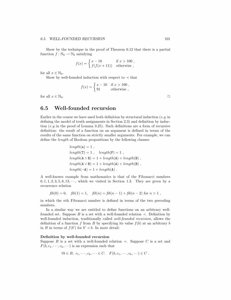
6.5. WELL-FOUNDED RECURSION 101
Show by the technique in the proof of Theorem 6.12 that there is a partialfunction f : N0 ⇀ N0 satisfying
f(x) ={x− 10 if x > 100 ,f(f(x+ 11)) otherwise ,
for all x ∈ N0.Show by well-founded induction with respect to ≺ that
f(x) ={x− 10 if x > 100 ,91 otherwise ,
for all x ∈ N0. 2
6.5 Well-founded recursion
Earlier in the course we have used both definition by structural induction (e.g. indefining the model of truth assignments in Section 2.3) and definition by induc-tion (e.g. in the proof of Lemma 3.25). Such definitions are a form of recursivedefinition: the result of a function on an argument is defined in terms of theresults of the same function on strictly smaller arguments. For example, we candefine the length of Boolean propositions by the following clauses:
length(a) = 1 ,length(T) = 1 , length(F) = 1 ,length(A ∧ B) = 1 + length(A) + length(B) ,length(A ∨ B) = 1 + length(A) + length(B) ,length(¬A) = 1 + length(A) .
A well-known example from mathematics is that of the Fibonacci numbers0, 1, 1, 2, 3, 5, 8, 13, · · ·, which we visited in Section 1.3. They are given by arecurrence relation
fib(0) = 0, fib(1) = 1, fib(n) = fib(n− 1) + fib(n− 2) for n > 1 ,
in which the nth Fibonacci number is defined in terms of the two precedingnumbers.
In a similar way we are entitled to define functions on an arbitrary well-founded set. Suppose B is a set with a well-founded relation ≺. Definition bywell-founded induction, traditionally called well-founded recursion, allows thedefinition of a function f from B by specifying its value f(b) at an arbitrary bin B in terms of f(b′) for b′ ≺ b. In more detail:
Definition by well-founded recursionSuppose B is a set with a well-founded relation ≺. Suppose C is a set andF (b, c1, · · · , ck, · · ·) is an expression such that
∀b ∈ B, c1, · · · , ck, · · · ∈ C. F (b, c1, · · · , ck, · · ·) ∈ C .
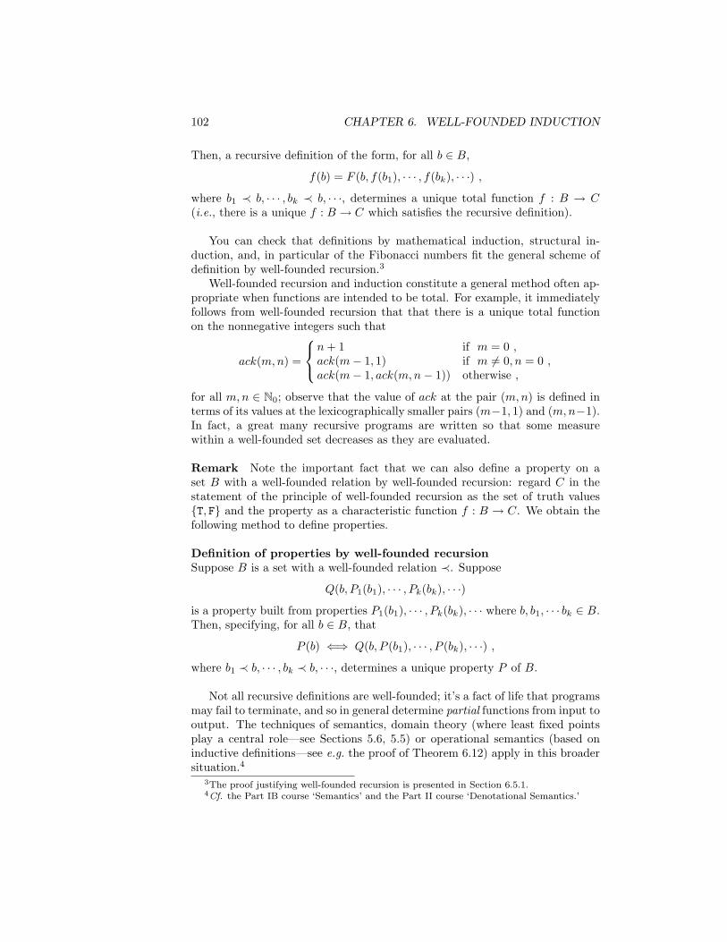
102 CHAPTER 6. WELL-FOUNDED INDUCTION
Then, a recursive definition of the form, for all b ∈ B,
f(b) = F (b, f(b1), · · · , f(bk), · · ·) ,
where b1 ≺ b, · · · , bk ≺ b, · · ·, determines a unique total function f : B → C(i.e., there is a unique f : B → C which satisfies the recursive definition).
You can check that definitions by mathematical induction, structural in-duction, and, in particular of the Fibonacci numbers fit the general scheme ofdefinition by well-founded recursion.3
Well-founded recursion and induction constitute a general method often ap-propriate when functions are intended to be total. For example, it immediatelyfollows from well-founded recursion that that there is a unique total functionon the nonnegative integers such that
ack(m,n) =
n+ 1 if m = 0 ,ack(m− 1, 1) if m 6= 0, n = 0 ,ack(m− 1, ack(m,n− 1)) otherwise ,
for all m,n ∈ N0; observe that the value of ack at the pair (m,n) is defined interms of its values at the lexicographically smaller pairs (m−1, 1) and (m,n−1).In fact, a great many recursive programs are written so that some measurewithin a well-founded set decreases as they are evaluated.
Remark Note the important fact that we can also define a property on aset B with a well-founded relation by well-founded recursion: regard C in thestatement of the principle of well-founded recursion as the set of truth values{T, F} and the property as a characteristic function f : B → C. We obtain thefollowing method to define properties.
Definition of properties by well-founded recursionSuppose B is a set with a well-founded relation ≺. Suppose
Q(b, P1(b1), · · · , Pk(bk), · · ·)
is a property built from properties P1(b1), · · · , Pk(bk), · · · where b, b1, · · · bk ∈ B.Then, specifying, for all b ∈ B, that
P (b) ⇐⇒ Q(b, P (b1), · · · , P (bk), · · ·) ,
where b1 ≺ b, · · · , bk ≺ b, · · ·, determines a unique property P of B.
Not all recursive definitions are well-founded; it’s a fact of life that programsmay fail to terminate, and so in general determine partial functions from input tooutput. The techniques of semantics, domain theory (where least fixed pointsplay a central role—see Sections 5.6, 5.5) or operational semantics (based oninductive definitions—see e.g. the proof of Theorem 6.12) apply in this broadersituation.4
3The proof justifying well-founded recursion is presented in Section 6.5.1.4Cf. the Part IB course ‘Semantics’ and the Part II course ‘Denotational Semantics.’
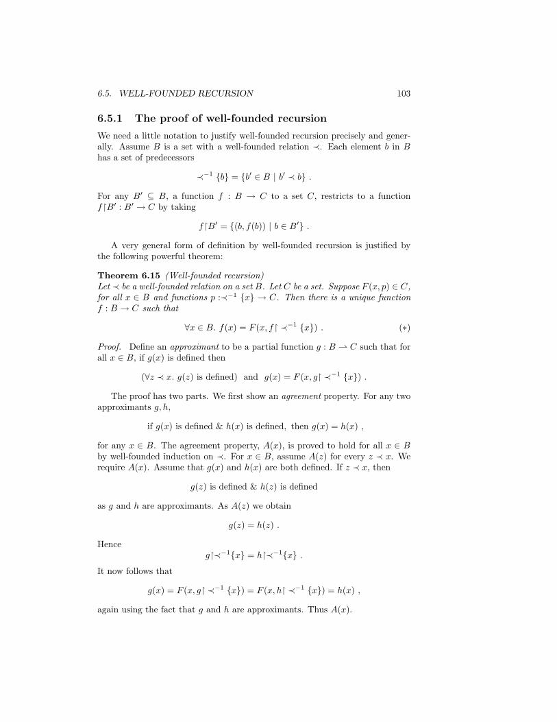
6.5. WELL-FOUNDED RECURSION 103
6.5.1 The proof of well-founded recursion
We need a little notation to justify well-founded recursion precisely and gener-ally. Assume B is a set with a well-founded relation ≺. Each element b in Bhas a set of predecessors
≺−1 {b} = {b′ ∈ B | b′ ≺ b} .
For any B′ ⊆ B, a function f : B → C to a set C, restricts to a functionf�B′ : B′ → C by taking
f�B′ = {(b, f(b)) | b ∈ B′} .
A very general form of definition by well-founded recursion is justified bythe following powerful theorem:
Theorem 6.15 (Well-founded recursion)Let ≺ be a well-founded relation on a set B. Let C be a set. Suppose F (x, p) ∈ C,for all x ∈ B and functions p :≺−1 {x} → C. Then there is a unique functionf : B → C such that
∀x ∈ B. f(x) = F (x, f� ≺−1 {x}) . (∗)
Proof. Define an approximant to be a partial function g : B ⇀ C such that forall x ∈ B, if g(x) is defined then
(∀z ≺ x. g(z) is defined) and g(x) = F (x, g� ≺−1 {x}) .
The proof has two parts. We first show an agreement property. For any twoapproximants g, h,
if g(x) is defined & h(x) is defined, then g(x) = h(x) ,
for any x ∈ B. The agreement property, A(x), is proved to hold for all x ∈ Bby well-founded induction on ≺. For x ∈ B, assume A(z) for every z ≺ x. Werequire A(x). Assume that g(x) and h(x) are both defined. If z ≺ x, then
g(z) is defined & h(z) is defined
as g and h are approximants. As A(z) we obtain
g(z) = h(z) .
Henceg�≺−1{x} = h�≺−1{x} .
It now follows that
g(x) = F (x, g� ≺−1 {x}) = F (x, h� ≺−1 {x}) = h(x) ,
again using the fact that g and h are approximants. Thus A(x).
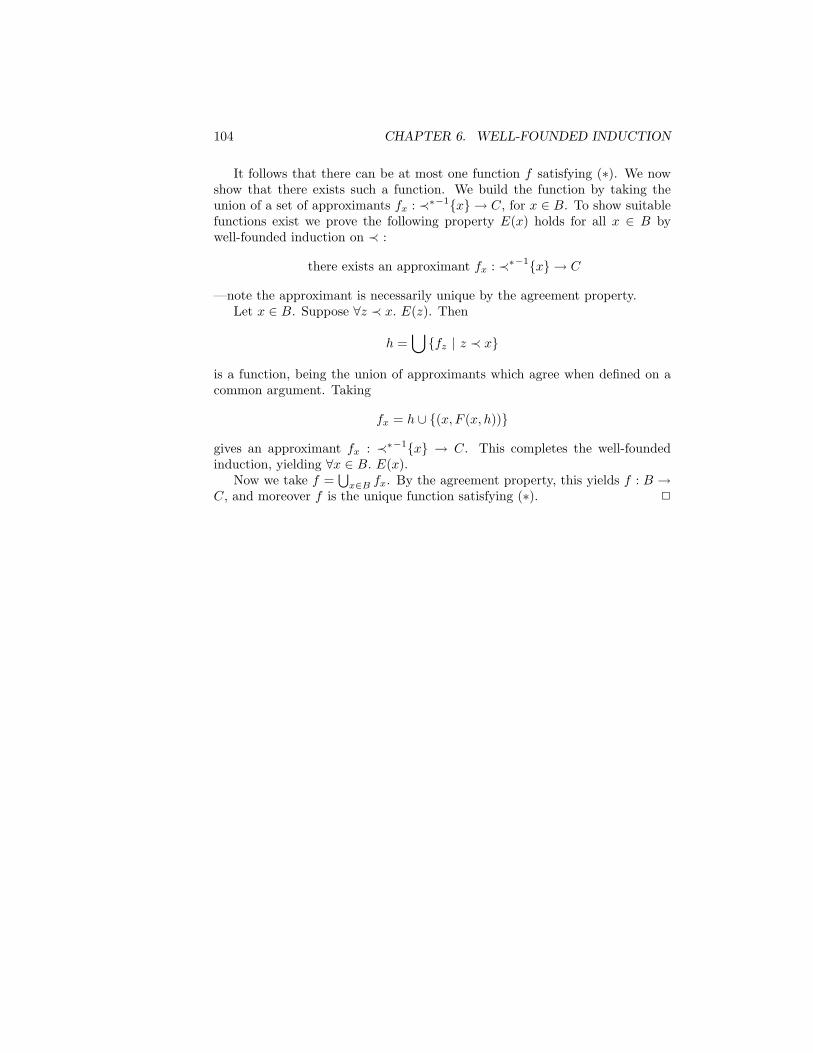
104 CHAPTER 6. WELL-FOUNDED INDUCTION
It follows that there can be at most one function f satisfying (∗). We nowshow that there exists such a function. We build the function by taking theunion of a set of approximants fx : ≺∗−1{x} → C, for x ∈ B. To show suitablefunctions exist we prove the following property E(x) holds for all x ∈ B bywell-founded induction on ≺ :
there exists an approximant fx : ≺∗−1{x} → C
—note the approximant is necessarily unique by the agreement property.Let x ∈ B. Suppose ∀z ≺ x. E(z). Then
h =⋃{fz | z ≺ x}
is a function, being the union of approximants which agree when defined on acommon argument. Taking
fx = h ∪ {(x, F (x, h))}
gives an approximant fx : ≺∗−1{x} → C. This completes the well-foundedinduction, yielding ∀x ∈ B. E(x).
Now we take f =⋃x∈B fx. By the agreement property, this yields f : B →
C, and moreover f is the unique function satisfying (∗). 2
Chapter 7
Inductively-defined classes
The inductive definition of properties and classes is derived from the earlierinductive definition of sets. The main example, the class of ordinals is definedinductively and shown to be strictly well-ordered. This leads to the methods oftransfinite induction and recursion. The methods are illustrated on a treatmentof cardinals as ordinals and in revisiting Tarski’s fixed-point theorem.
7.1 Sets, properties and classes
Sets, possibly as here with basic assumed elements, form the universe of dis-course of set theory. And we learn to think of sets as elements themselves, outof which we build even larger sets. We have also learnt to be cautious aboutthose collections we take to be sets, and in Chapter 4 have prescribed safe waysto construct sets.
However, mathematical practice also seeks convenience. It is very commonto treat very general properties in a set-like way, even though the collectionsassociated with those properties are not ensured to be sets. Collections whichneed not be sets are called classes, and classes form a convenient way to describeand handle properties. A property P (x) determines a class C = {x | P (x)}, andwe can as an alternative to saying P (u) say u ∈ C. For example, the property‘x is a set with three distinct elements’ is associated with the class of all setswith precisely three elements. Perhaps more dangerously, the property ‘x is aset which is not a member of itself’ is associated with the class of all sets xfor which x /∈ x; according to the axiom of foundation no set is a member ofitself, so this class would coincide with the class of all sets. Notice we escapeRussell’s paradox by not taking this class to be a set; this distinction of type,originating in the work of Russell and Whitehead, blocks the argument leadingto the paradox.
This view of properties as classes carries with it an assumption that proper-ties are equivalent iff they are associated with the same class, i.e. are satisfiedby exactly the same elements. It also leads to saying a property P is stronger
105
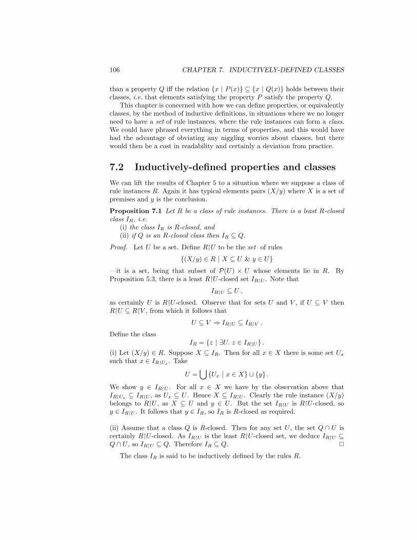
106 CHAPTER 7. INDUCTIVELY-DEFINED CLASSES
than a property Q iff the relation {x | P (x)} ⊆ {x | Q(x)} holds between theirclasses, i.e. that elements satisfying the property P satisfy the property Q.
This chapter is concerned with how we can define properties, or equivalentlyclasses, by the method of inductive definitions, in situations where we no longerneed to have a set of rule instances, where the rule instances can form a class.We could have phrased everything in terms of properties, and this would havehad the advantage of obviating any niggling worries about classes, but therewould then be a cost in readability and certainly a deviation from practice.
7.2 Inductively-defined properties and classes
We can lift the results of Chapter 5 to a situation where we suppose a class ofrule instances R. Again it has typical elements pairs (X/y) where X is a set ofpremises and y is the conclusion.
Proposition 7.1 Let R be a class of rule instances. There is a least R-closedclass IR, i.e.
(i) the class IR is R-closed, and(ii) if Q is an R-closed class then IR ⊆ Q.
Proof. Let U be a set. Define R�U to be the set of rules
{(X/y) ∈ R | X ⊆ U & y ∈ U}
—it is a set, being that subset of P(U) × U whose elements lie in R. ByProposition 5.3, there is a least R�U -closed set IR�U . Note that
IR�U ⊆ U ,
as certainly U is R�U -closed. Observe that for sets U and V , if U ⊆ V thenR�U ⊆ R�V , from which it follows that
U ⊆ V ⇒ IR�U ⊆ IR�V .
Define the classIR = {z | ∃U. z ∈ IR�U} .
(i) Let (X/y) ∈ R. Suppose X ⊆ IR. Then for all x ∈ X there is some set Uxsuch that x ∈ IR�Ux . Take
U =⋃{Ux | x ∈ X} ∪ {y} .
We show y ∈ IR�U . For all x ∈ X we have by the observation above thatIR�Ux ⊆ IR�U , as Ux ⊆ U . Hence X ⊆ IR�U . Clearly the rule instance (X/y)belongs to R�U , as X ⊆ U and y ∈ U . But the set IR�U is R�U -closed, soy ∈ IR�U . It follows that y ∈ IR, so IR is R-closed as required.
(ii) Assume that a class Q is R-closed. Then for any set U , the set Q ∩ U iscertainly R�U -closed. As IR�U is the least R�U -closed set, we deduce IR�U ⊆Q ∩ U , so IR�U ⊆ Q. Therefore IR ⊆ Q. 2
The class IR is said to be inductively defined by the rules R.
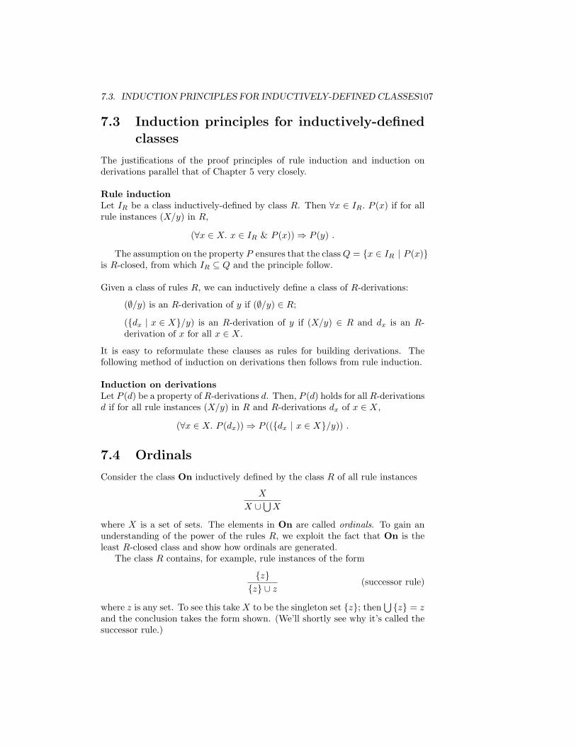
7.3. INDUCTION PRINCIPLES FOR INDUCTIVELY-DEFINED CLASSES107
7.3 Induction principles for inductively-definedclasses
The justifications of the proof principles of rule induction and induction onderivations parallel that of Chapter 5 very closely.
Rule inductionLet IR be a class inductively-defined by class R. Then ∀x ∈ IR. P (x) if for allrule instances (X/y) in R,
(∀x ∈ X. x ∈ IR & P (x))⇒ P (y) .
The assumption on the property P ensures that the classQ = {x ∈ IR | P (x)}is R-closed, from which IR ⊆ Q and the principle follow.
Given a class of rules R, we can inductively define a class of R-derivations:
(∅/y) is an R-derivation of y if (∅/y) ∈ R;
({dx | x ∈ X}/y) is an R-derivation of y if (X/y) ∈ R and dx is an R-derivation of x for all x ∈ X.
It is easy to reformulate these clauses as rules for building derivations. Thefollowing method of induction on derivations then follows from rule induction.
Induction on derivationsLet P (d) be a property of R-derivations d. Then, P (d) holds for all R-derivationsd if for all rule instances (X/y) in R and R-derivations dx of x ∈ X,
(∀x ∈ X. P (dx))⇒ P (({dx | x ∈ X}/y)) .
7.4 Ordinals
Consider the class On inductively defined by the class R of all rule instances
X
X ∪⋃X
where X is a set of sets. The elements in On are called ordinals. To gain anunderstanding of the power of the rules R, we exploit the fact that On is theleast R-closed class and show how ordinals are generated.
The class R contains, for example, rule instances of the form
{z}{z} ∪ z
(successor rule)
where z is any set. To see this take X to be the singleton set {z}; then⋃{z} = z
and the conclusion takes the form shown. (We’ll shortly see why it’s called thesuccessor rule.)
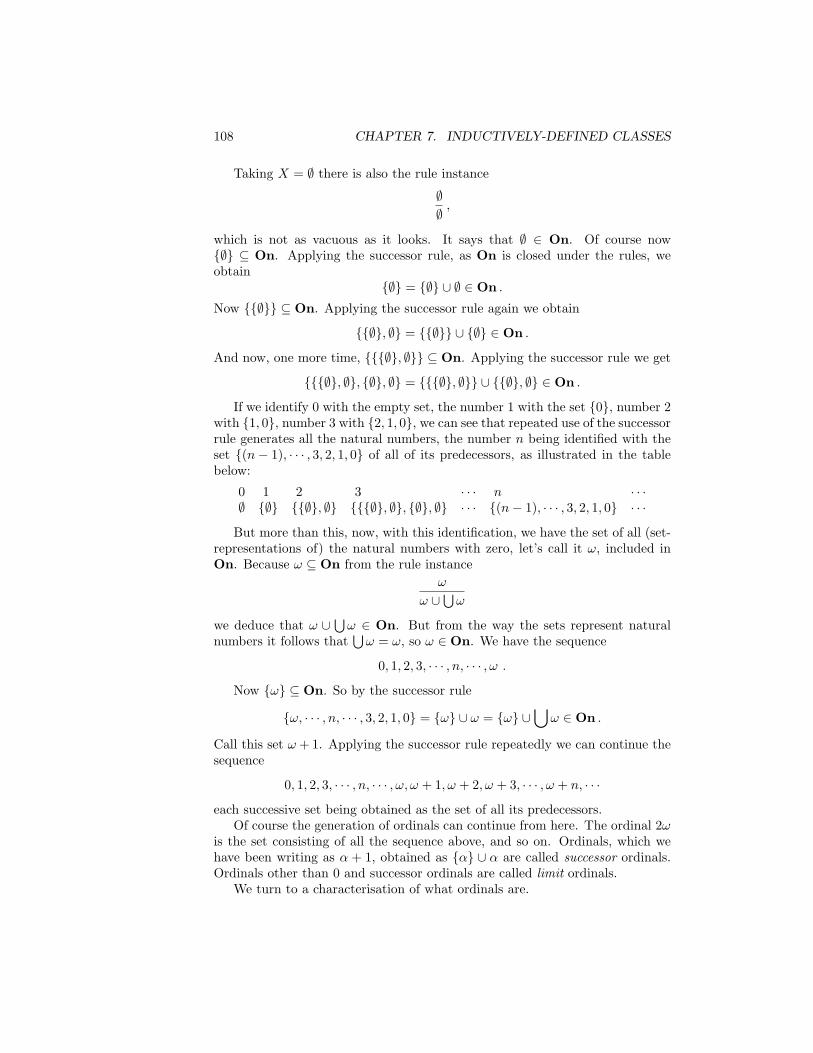
108 CHAPTER 7. INDUCTIVELY-DEFINED CLASSES
Taking X = ∅ there is also the rule instance
∅∅,
which is not as vacuous as it looks. It says that ∅ ∈ On. Of course now{∅} ⊆ On. Applying the successor rule, as On is closed under the rules, weobtain
{∅} = {∅} ∪ ∅ ∈ On .
Now {{∅}} ⊆ On. Applying the successor rule again we obtain
{{∅}, ∅} = {{∅}} ∪ {∅} ∈ On .
And now, one more time, {{{∅}, ∅}} ⊆ On. Applying the successor rule we get
{{{∅}, ∅}, {∅}, ∅} = {{{∅}, ∅}} ∪ {{∅}, ∅} ∈ On .
If we identify 0 with the empty set, the number 1 with the set {0}, number 2with {1, 0}, number 3 with {2, 1, 0}, we can see that repeated use of the successorrule generates all the natural numbers, the number n being identified with theset {(n− 1), · · · , 3, 2, 1, 0} of all of its predecessors, as illustrated in the tablebelow:
0 1 2 3 · · · n · · ·∅ {∅} {{∅}, ∅} {{{∅}, ∅}, {∅}, ∅} · · · {(n− 1), · · · , 3, 2, 1, 0} · · ·
But more than this, now, with this identification, we have the set of all (set-representations of) the natural numbers with zero, let’s call it ω, included inOn. Because ω ⊆ On from the rule instance
ω
ω ∪⋃ω
we deduce that ω ∪⋃ω ∈ On. But from the way the sets represent natural
numbers it follows that⋃ω = ω, so ω ∈ On. We have the sequence
0, 1, 2, 3, · · · , n, · · · , ω .
Now {ω} ⊆ On. So by the successor rule
{ω, · · · , n, · · · , 3, 2, 1, 0} = {ω} ∪ ω = {ω} ∪⋃ω ∈ On .
Call this set ω + 1. Applying the successor rule repeatedly we can continue thesequence
0, 1, 2, 3, · · · , n, · · · , ω, ω + 1, ω + 2, ω + 3, · · · , ω + n, · · ·
each successive set being obtained as the set of all its predecessors.Of course the generation of ordinals can continue from here. The ordinal 2ω
is the set consisting of all the sequence above, and so on. Ordinals, which wehave been writing as α + 1, obtained as {α} ∪ α are called successor ordinals.Ordinals other than 0 and successor ordinals are called limit ordinals.
We turn to a characterisation of what ordinals are.
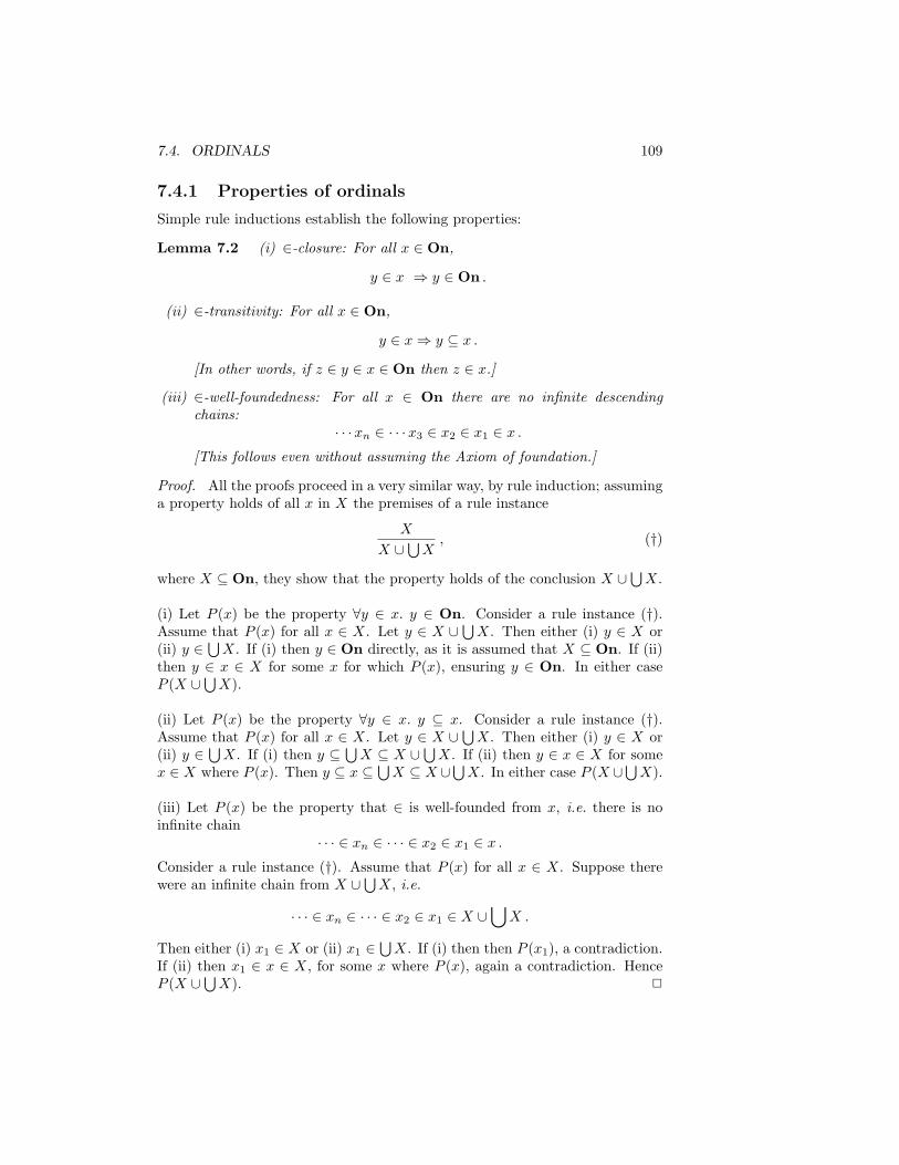
7.4. ORDINALS 109
7.4.1 Properties of ordinals
Simple rule inductions establish the following properties:
Lemma 7.2 (i) ∈-closure: For all x ∈ On,
y ∈ x ⇒ y ∈ On .
(ii) ∈-transitivity: For all x ∈ On,
y ∈ x⇒ y ⊆ x .
[In other words, if z ∈ y ∈ x ∈ On then z ∈ x.]
(iii) ∈-well-foundedness: For all x ∈ On there are no infinite descendingchains:
· · ·xn ∈ · · ·x3 ∈ x2 ∈ x1 ∈ x .[This follows even without assuming the Axiom of foundation.]
Proof. All the proofs proceed in a very similar way, by rule induction; assuminga property holds of all x in X the premises of a rule instance
X
X ∪⋃X, (†)
where X ⊆ On, they show that the property holds of the conclusion X ∪⋃X.
(i) Let P (x) be the property ∀y ∈ x. y ∈ On. Consider a rule instance (†).Assume that P (x) for all x ∈ X. Let y ∈ X ∪
⋃X. Then either (i) y ∈ X or
(ii) y ∈⋃X. If (i) then y ∈ On directly, as it is assumed that X ⊆ On. If (ii)
then y ∈ x ∈ X for some x for which P (x), ensuring y ∈ On. In either caseP (X ∪
⋃X).
(ii) Let P (x) be the property ∀y ∈ x. y ⊆ x. Consider a rule instance (†).Assume that P (x) for all x ∈ X. Let y ∈ X ∪
⋃X. Then either (i) y ∈ X or
(ii) y ∈⋃X. If (i) then y ⊆
⋃X ⊆ X ∪
⋃X. If (ii) then y ∈ x ∈ X for some
x ∈ X where P (x). Then y ⊆ x ⊆⋃X ⊆ X ∪
⋃X. In either case P (X ∪
⋃X).
(iii) Let P (x) be the property that ∈ is well-founded from x, i.e. there is noinfinite chain
· · · ∈ xn ∈ · · · ∈ x2 ∈ x1 ∈ x .Consider a rule instance (†). Assume that P (x) for all x ∈ X. Suppose therewere an infinite chain from X ∪
⋃X, i.e.
· · · ∈ xn ∈ · · · ∈ x2 ∈ x1 ∈ X ∪⋃X .
Then either (i) x1 ∈ X or (ii) x1 ∈⋃X. If (i) then then P (x1), a contradiction.
If (ii) then x1 ∈ x ∈ X, for some x where P (x), again a contradiction. HenceP (X ∪
⋃X). 2
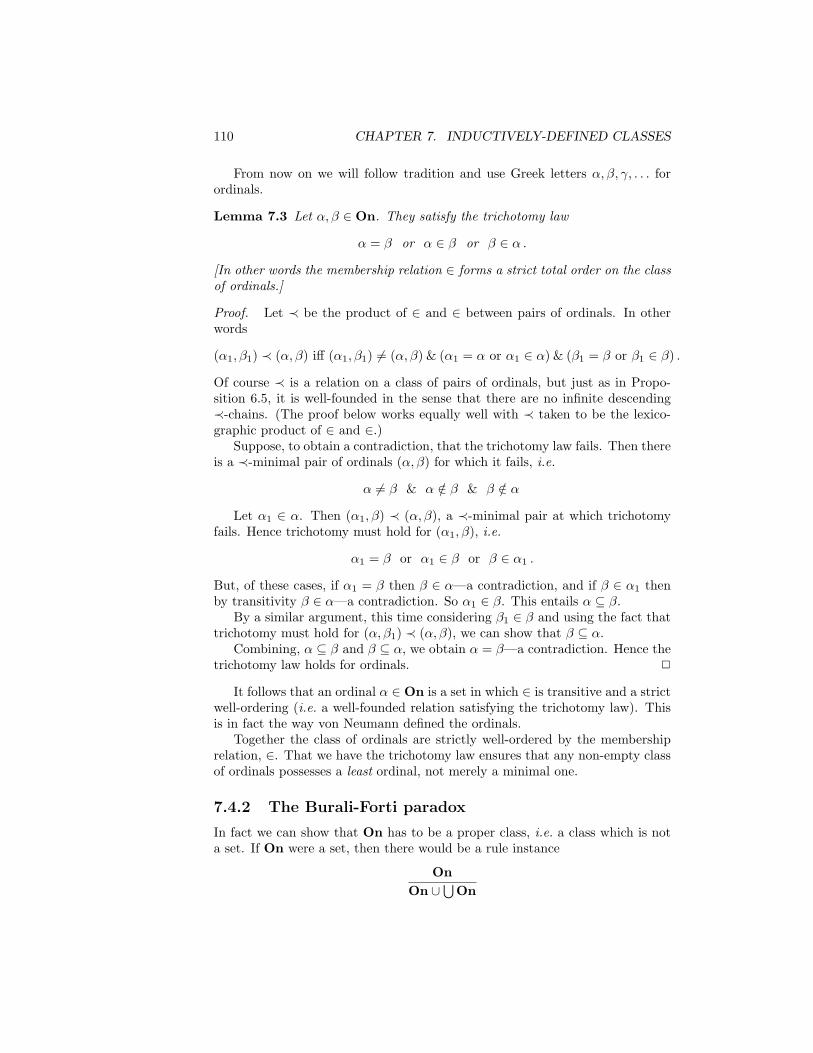
110 CHAPTER 7. INDUCTIVELY-DEFINED CLASSES
From now on we will follow tradition and use Greek letters α, β, γ, . . . forordinals.
Lemma 7.3 Let α, β ∈ On. They satisfy the trichotomy law
α = β or α ∈ β or β ∈ α .
[In other words the membership relation ∈ forms a strict total order on the classof ordinals.]
Proof. Let ≺ be the product of ∈ and ∈ between pairs of ordinals. In otherwords
(α1, β1) ≺ (α, β) iff (α1, β1) 6= (α, β) & (α1 = α or α1 ∈ α) & (β1 = β or β1 ∈ β) .
Of course ≺ is a relation on a class of pairs of ordinals, but just as in Propo-sition 6.5, it is well-founded in the sense that there are no infinite descending≺-chains. (The proof below works equally well with ≺ taken to be the lexico-graphic product of ∈ and ∈.)
Suppose, to obtain a contradiction, that the trichotomy law fails. Then thereis a ≺-minimal pair of ordinals (α, β) for which it fails, i.e.
α 6= β & α /∈ β & β /∈ α
Let α1 ∈ α. Then (α1, β) ≺ (α, β), a ≺-minimal pair at which trichotomyfails. Hence trichotomy must hold for (α1, β), i.e.
α1 = β or α1 ∈ β or β ∈ α1 .
But, of these cases, if α1 = β then β ∈ α—a contradiction, and if β ∈ α1 thenby transitivity β ∈ α—a contradiction. So α1 ∈ β. This entails α ⊆ β.
By a similar argument, this time considering β1 ∈ β and using the fact thattrichotomy must hold for (α, β1) ≺ (α, β), we can show that β ⊆ α.
Combining, α ⊆ β and β ⊆ α, we obtain α = β—a contradiction. Hence thetrichotomy law holds for ordinals. 2
It follows that an ordinal α ∈ On is a set in which ∈ is transitive and a strictwell-ordering (i.e. a well-founded relation satisfying the trichotomy law). Thisis in fact the way von Neumann defined the ordinals.
Together the class of ordinals are strictly well-ordered by the membershiprelation, ∈. That we have the trichotomy law ensures that any non-empty classof ordinals possesses a least ordinal, not merely a minimal one.
7.4.2 The Burali-Forti paradox
In fact we can show that On has to be a proper class, i.e. a class which is nota set. If On were a set, then there would be a rule instance
OnOn ∪
⋃On
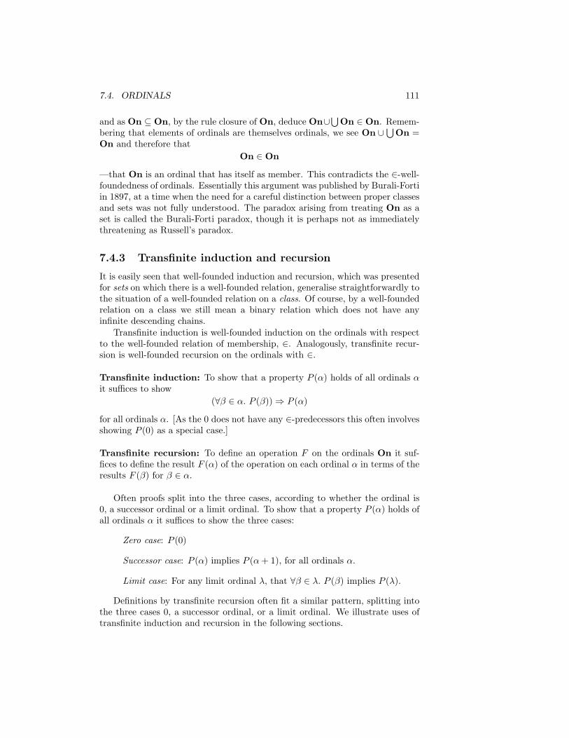
7.4. ORDINALS 111
and as On ⊆ On, by the rule closure of On, deduce On∪⋃
On ∈ On. Remem-bering that elements of ordinals are themselves ordinals, we see On ∪
⋃On =
On and therefore thatOn ∈ On
—that On is an ordinal that has itself as member. This contradicts the ∈-well-foundedness of ordinals. Essentially this argument was published by Burali-Fortiin 1897, at a time when the need for a careful distinction between proper classesand sets was not fully understood. The paradox arising from treating On as aset is called the Burali-Forti paradox, though it is perhaps not as immediatelythreatening as Russell’s paradox.
7.4.3 Transfinite induction and recursion
It is easily seen that well-founded induction and recursion, which was presentedfor sets on which there is a well-founded relation, generalise straightforwardly tothe situation of a well-founded relation on a class. Of course, by a well-foundedrelation on a class we still mean a binary relation which does not have anyinfinite descending chains.
Transfinite induction is well-founded induction on the ordinals with respectto the well-founded relation of membership, ∈. Analogously, transfinite recur-sion is well-founded recursion on the ordinals with ∈.
Transfinite induction: To show that a property P (α) holds of all ordinals αit suffices to show
(∀β ∈ α. P (β))⇒ P (α)
for all ordinals α. [As the 0 does not have any ∈-predecessors this often involvesshowing P (0) as a special case.]
Transfinite recursion: To define an operation F on the ordinals On it suf-fices to define the result F (α) of the operation on each ordinal α in terms of theresults F (β) for β ∈ α.
Often proofs split into the three cases, according to whether the ordinal is0, a successor ordinal or a limit ordinal. To show that a property P (α) holds ofall ordinals α it suffices to show the three cases:
Zero case: P (0)
Successor case: P (α) implies P (α+ 1), for all ordinals α.
Limit case: For any limit ordinal λ, that ∀β ∈ λ. P (β) implies P (λ).
Definitions by transfinite recursion often fit a similar pattern, splitting intothe three cases 0, a successor ordinal, or a limit ordinal. We illustrate uses oftransfinite induction and recursion in the following sections.
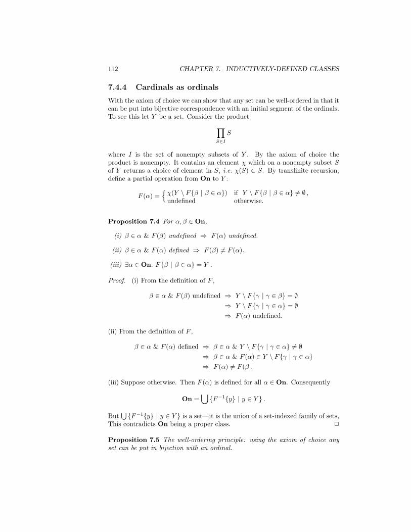
112 CHAPTER 7. INDUCTIVELY-DEFINED CLASSES
7.4.4 Cardinals as ordinals
With the axiom of choice we can show that any set can be well-ordered in that itcan be put into bijective correspondence with an initial segment of the ordinals.To see this let Y be a set. Consider the product∏
S∈IS
where I is the set of nonempty subsets of Y . By the axiom of choice theproduct is nonempty. It contains an element χ which on a nonempty subset Sof Y returns a choice of element in S, i.e. χ(S) ∈ S. By transfinite recursion,define a partial operation from On to Y :
F (α) ={χ(Y \ F{β | β ∈ α}) if Y \ F{β | β ∈ α} 6= ∅ ,undefined otherwise.
Proposition 7.4 For α, β ∈ On,
(i) β ∈ α & F (β) undefined ⇒ F (α) undefined.
(ii) β ∈ α & F (α) defined ⇒ F (β) 6= F (α).
(iii) ∃α ∈ On. F{β | β ∈ α} = Y .
Proof. (i) From the definition of F ,
β ∈ α & F (β) undefined ⇒ Y \ F{γ | γ ∈ β} = ∅⇒ Y \ F{γ | γ ∈ α} = ∅⇒ F (α) undefined.
(ii) From the definition of F ,
β ∈ α & F (α) defined ⇒ β ∈ α & Y \ F{γ | γ ∈ α} 6= ∅⇒ β ∈ α & F (α) ∈ Y \ F{γ | γ ∈ α}⇒ F (α) 6= F (β .
(iii) Suppose otherwise. Then F (α) is defined for all α ∈ On. Consequently
On =⋃{F−1{y} | y ∈ Y } .
But⋃{F−1{y} | y ∈ Y } is a set—it is the union of a set-indexed family of sets,
This contradicts On being a proper class. 2
Proposition 7.5 The well-ordering principle: using the axiom of choice anyset can be put in bijection with an ordinal.
7.4. ORDINALS 113
Proof. Referring to Proposition 7.4, the domain of definition of F is not thewhole of On, but rather the initial segment of ordinals belonging to some ordinalα. Restricting F to its domain of definition α, we obtain a bijection betweenthe elements of an ordinal α and the set Y . 2
We can define the cardinality of a set Y as the least ordinal which, treatedas a set, is in bijection with Y . We define cardinals as those ordinals γ whichare not in bijection with any strictly smaller ordinal γ′ ∈ γ. Infinite cardinalsform an unbounded chain in the ordinals, starting
ℵ0 ∈ ℵ1 ∈ ℵ2 ∈ · · ·
The first infinite cardinal ℵ0 coincides with ω. It might be conjectured, asCantor did in 1877, that the next infinite cardinal ℵ1 is that of the set of realnumbers R. This conjecture, that
there is no cardinal strictly between that of the integers and that ofthe real numbers,
is called the continuum hypothesis. In fact, Godel and Cohen showed the con-tinuum hypothesis was independent of the usual axioms of set theory: that thecontinuum hypothesis is consistent with the axioms of set theory (Godel, 1940),and that its negation is consistent with the axioms (Cohen via the innovativetechnique of forcing, 1963).
7.4.5 Tarski’s fixed point theorem revisited
We extend the results of Section 5.6. Let U be a set and assume
ϕ : P(U)→ P(U)
is monotonic, i.e. such that
S ⊆ S′ ⇒ ϕ(S) ⊆ ϕ(S′) ,
for S, S′ ∈ P(U). Then ϕ has a minimum fixed point µX.ϕ(X) and a maximumfixed point as νX.ϕ(X). We first provide another way to construct the leastfixed point.
By transfinite recursion we define ϕα(∅) for an ordinal α:
ϕα(∅) =⋃β∈α
ϕ(ϕβ(∅)) .
It is obvious that the approximations form an increasing chain:
γ ∈ α⇒ ϕγ(∅) ⊆ ϕα(∅) .
To understand the definition better let’s see what it amounts to in the caseswhere α is zero, a successor or a limit ordinal. In the zero case
ϕ0(∅) = ∅ ,
114 CHAPTER 7. INDUCTIVELY-DEFINED CLASSES
as an empty union is the empty set. In the successor case
ϕα+1(∅) =⋃
β∈α+1
ϕ(ϕβ(∅)) = ϕ(ϕα(∅) ,
using the monotonicity of ϕ and that the approximations ϕβ(∅), for β ∈ α+ 1,are all dominated by ϕα(∅). In the case of a limit ordinal λ,
ϕλ(∅) =⋃β∈λ
ϕ(ϕβ(∅)) =⋃β∈λ
ϕβ+1(∅) ∪ ϕ0(∅) =⋃β∈λ
ϕβ(∅)
Here we have used the fact that for a limit ordinal λ, if β ∈ λ then β + 1 ∈ λ—otherwise λ would be the successor ordinal β + 1.
So we could have given an equivalent definition of ϕα(∅) by the followingclauses of a transfinite recursion:
Zero case: ϕ0(∅) = ∅ .
Successor case: ϕα+1(∅) = ϕ(ϕα(∅)) .
Limit case: ϕλ(∅) =⋃α∈λ ϕ
α(∅) .
Though with this alternative definition we would have had to work a little harderto show that the approximations increased.
Once we have all the approximations we will find that the minimum fixedpoint
µX.ϕ(X) =⋃
α∈On
ϕα(∅) .
At first sight it is not even obvious that the union forms a set—it is indexed bya class of ordinals. However, there must be some ordinal γ at which ϕγ+1(∅) =ϕγ(∅), so µX.ϕ(X) = ϕγ(∅)—the least such ordinal is called the closure ordinalof ϕ. Otherwise there would be a way to map a subset of U onto the ordinals On.This would be a way to index the ordinals by a set, from which On would be aset—a contradiction. Clearly ϕγ(∅), so µX.ϕ(X), is a fixed point of ϕ. That itis the minimum fixed point (indeed minimum prefixed point) now follows by astraightforward transfinite induction on the approximants ϕα(∅).
Exercise 7.6 Spell out the argument that⋃α∈On ϕ
α(∅) above forms a set.Prove that µX.ϕ(X) is the minimum prefixed point of ϕ : P(U)→ P(U).
Note that in a precisely dual fashion, one can express a maximum fixed pointas the intersection of ordinal-indexed approximations.
Exercise 7.7 Explain how to express a maximum fixed point of a monotonicfunction ϕ : P(U) → P(U) as the intersection of ordinal-indexed approxima-tions.
7.5. THE CUMULATIVE HIERARCHY 115
7.5 The cumulative hierarchy
One use of ordinals is to stratify sets according to depth of the nesting of theirelements. If we start building sets just from the empty set this yields thecumulative hierarchy, or von Neumann hierarchy of sets, a way to rank the setsassumed in Zermelo-Fraenkel set theory.
Define Vα, for an ordinal α, by transfinite recursion:
V∅ is the empty set, ∅;
Vβ+1 = P(Vβ), the power set of Vβ , for any ordinal β;
Vλ =⋃β∈λ Vβ , for any limit ordinal λ.
The class V is the union of all the Vα-stages:
V =def
⋃α
Vα .
The rank of a set in x ∈ V is the least ordinal ρ for which x ∈ Vρ.
The sets V form the sets of Zermelo-Fraenkel set theory. Zermelo-Fraenkelset theory is a development of set theory like that of these notes, but wherethere are no elements assumed from the start. This doesn’t stop constructingthe empty set, and then sets containing the empty set, and so on. A simpletransfinite induction shows that each set in V is well-founded, in the sense thatthe binary relation ∈ is a well-founded relation on the set. In other words, fromthe nature of their construction, the set theory based on V naturally satisfiesthe axiom of foundation.
In particular, for any set x ∈ V we must have x /∈ x. This can furnish a trickwhich is occasionally useful. Suppose we have a set x and we want to adjoinsome new fresh element not already in x. Then the element x presents itselfas a canonical candidate. Forming x ∪ {x} we are sure to have adjoined a newelement to the set x.
Choices of fresh names, e.g. in naming fresh variables or fresh values, areimportant in Computer Science, both in syntax and semantics, and we turn inthe next chapter to a less ad hoc, more thorough and general treatment of freshnames, a treatment that takes seriously the essential symmetry there is betweendifferent choices of fresh name.
Exercise 7.8(i) Show by transfinite induction that each Vα, α ∈ On, is transitive, i.e.
x ∈ y ∈ Vα ⇒ x ∈ Vα ,
(equivalently, that y ∈ Vα ⇒ y ⊆ Vα).(ii) Show, for α, β ∈ On,
α ⊆ β ⇒ Vα ⊆ Vβ
116 CHAPTER 7. INDUCTIVELY-DEFINED CLASSES
(Use transfinite induction on β).(iii) Show by transfinite induction that α ⊆ Vα, or equivalently that α ∈ Vα+1,for α ∈ On. 2
Chapter 8
Fraenkel-Mostowski sets
This chapter is rough and incomplete.Classes with an action. Fraenkel-Mostowski (FM) sets. Nominal sets. FM-
set constructions. Failure of the axiom of choice. Freshness. A separatingproduct and new-name abstraction on nominal sets.
8.1 Atoms and permutations
Assume an infinite set of atoms A. Let Perm consist of those finite permutationsπ of A which are fixed on all but a finite set of names. Permutations π are specialbijective functions π : A → A. As such we compose them as functions as it isclear that the composition of permutations is a permutation. As a bijection, apermutation π possesses an inverse permutation π−1.
A cycle (a1a2 · · · an) consists of a finite sequence of distinct atoms and standsfor the permutation: a1 7→ a2, a2 7→ a3, . . . , an 7→ a1. It is well known thata permutation π ∈ Perm can be expressed as the composition of cycles, wherethe order of the cycles in the composition is unimportant; a typical cycle is gotby repeatedly applying π to an atom a not fixed by π.
A transposition (ab) is a permutation swapping a with b, and b with a. Notewhen a = b then a transposition (ab) acts as the identity permutation. We say(ab) is a proper transposition when a 6= b. Proper transpositions are the sameas 2-cycles. A cycle (a1a2 · · · an) can be expressed as a composition of propertranspositions:
(a1a2 · · · an) = (a1an)(a1an−1) · · · (a1a3)(a1a2) .
Consequently any permutation can be obtained as the composition of propertranspositions.
Proposition 8.1 Let π ∈ Perm and a, b ∈ A. Then,
π ◦ (ab) = (π(a)π(b)) ◦ π .
117
118 CHAPTER 8. FRAENKEL-MOSTOWSKI SETS
8.2 Classes with an action
This section assembles some general facts about classes with an action.Throughout this section we assume a class with an action, comprising (X, ·)
where X is a class and π · x ∈ X, for π ∈ Perm and x ∈ X, satisfies
idA · x = x and π1 · (π2 · x) = (π1 ◦ π2) · x .
An element x ∈ X has support A ⊆ A when for all π ∈ Perm for which ∀a ∈A. π(a) = a we have π · x = x; we say x has finite support when A is finite. Inother words, an element has support A when every permutation which fixes allatoms in A also fixes x.
Proposition 8.2 Let π ∈ Perm. If x ∈ X has support A, then π · x has supportπA.
Proof. Assume x has support A. Suppose σ ∈ Perm fixes all atoms in πA.Then π−1 ◦ σ ◦ π fixes all atoms in A, so
π−1 · σ · π · x = x ,
and hence σ · π · x = π · x. 2
Because every permutation can be written as the composition of transpo-sitions, we can immediately express the concept of support just in terms oftranspositions.
Proposition 8.3 Let A be a subset of atoms. A proper transposition (ab) fixesall atoms in A iff a /∈ A and b /∈ A.
An element x ∈ X has support A ⊆ A iff (ab) · x = x for all (distinct)a, b /∈ A.
Example: (A, ·) where π · a = π(a). The smallest support of a ∈ A is {a}.
Example: (Perm, ·) where π · σ = π◦σ◦π−1. The smallest support of σ ∈ Permis {a ∈ A | σ(a) 6= a}****
Proposition 8.4 Finite subsets A ⊆ A have finite support A. Cofinite subsetsA \ A, where A is a finite subset A ⊆ A, have finite support A; infinite subsetswhich are not cofinite do not have finite support.
***note that supersets of cofinite subsets of A are cofinite*****
Lemma 8.5 If x ∈ X has finite support A1 and also has finite support A2 thenx has support A1 ∩A2.
8.3. FRAENKEL-MOSTOWSKI SETS 119
Proof. Assume that x both has support A1 and A2. Let (b1b2) be a propertransposition which fixes all atoms in A1 ∩ A2. We show that (b1b2) also fixesx, i.e. (b1b2) · x = x.
Because (b1b2) fixes all atoms in A1 ∩ A2, we know b1, b2 /∈ A1 ∩ A2. Ifb1, b2 /∈ A1 or b1, b2 /∈ A2 then (b1b2) would either fix all atoms in A1 or allatoms in A2; in either case (b1b2) fixes x. So suppose otherwise, whence either(i) b1 ∈ A1 \ A2 and b2 ∈ A2 \ A1 or (ii) b2 ∈ A1 \ A2 and b1 ∈ A2 \ A1.Consider case (i)—the argument in case (ii) is similar. Take c to be an atomnot in A1 ∪A2. Then it can be checked that
(b1b2) = (b1c)(b2c)(b1c) .
As b1, c /∈ A2 the transposition (b1c) fixes all atoms in A2 and hence x. Sim-ilarly, as b2, c /∈ A1 the transposition (b2c) fixes all atoms in A1 and hence x.Consequently, (b1b2), got as their composition, fixes x. 2
Corollary 8.6 If x ∈ X has finite support, then it has a minimum finite sup-port.
Proof. Suppose x has finite support A0. The minimum support is given by⋂{A | x has support A} which is equal to the finite intersection of supports
within A0. 2
Definition: If x has finite support, we write supp(x) for the minimum supportof x.
Lemma 8.7 For a, b ∈ A, and x ∈ X with finite support,
a /∈ supp(x) & b ∈ supp(x)⇒ (ab) · x 6= x .
Proof. The element x has minimum support supp(x). Therefore, by Propo-sition 8.2, (ab) · x has support (ab) · supp(x), which does not contain b. If(ab) · x = x then x would have a support not containing b—a contradiction. 2
8.3 Fraenkel-Mostowski sets
Fraenkel-Mostowski (FM) sets are sets built up by starting from an infinite,finitely-permutable set of atoms. The permutation of atoms induces a permuta-tion action on FM sets. Initially we will imitate the construction of the cumu-lative hierarchy in Section 7.5, but starting from a set of atoms, and ignoringtheir permutability.
We first build a hierarchy of sets on the infinite set of atoms A by transfiniterecursion:
• U0 = A;
• Uα+1 = Uα ∪ P(Uα);
120 CHAPTER 8. FRAENKEL-MOSTOWSKI SETS
• Uλ =⋃α∈λ Uα.
Define the class of sets built on atoms A to be U =⋃α∈On Uα.
Proposition 8.8 (i) For all α ∈ On,
x ∈ y ∈ Uα ⇒ x ∈ Uα .
(ii) For all α, β ∈ On,α ⊆ β ⇒ Uα ⊆ Uβ .
(iii) The membership relation ∈ is well-founded in U , i.e. there are no infinitedescending chains
· · · ∈ xn ∈ · · · ∈ x1 ∈ x0
in U .
Proof. By transfinite inductions. 2
Define an action on U by well-founded induction on ∈:
• π · a = π(a) when a ∈ A;
• π · x = {π · y | y ∈ x} when x ∈ U is not in A.
By well-founded induction on ∈, it can be shown that
idA · x = x and π1 · (π2 · x) = (π1 ◦ π2) · x .
Thus U with the operation · is an example of a class with an action. From itsdefinition, the action respects membership:
if x ∈ y then π · x ∈ π · y ,
for any x, y ∈ U and π ∈ Perm.
Proposition 8.9 Let x ∈ U and π ∈ Perm. Then, π · x = x iff π · x ⊆ x.
Proof. The “Only if” direction is clear. “If”: Suppose π · x ⊆ x and, to obtaina contradiction, that π · x 6= x, i.e. π · x ( x. Note that action is monotonic inthe sense that if y ⊆ z in U then π · y ⊆ π · z. Hence, by a simple mathematicalinduction, πn · x ( x for all n ≥ 1. But π is a finite permutation of A soπk = idA for some k. This yields the contradiction πk · x = idA · x = x. 2
Now we can define the Fraenkel-Mostowski sets.
Definition: Define the property of being an Fraenkel-Mostowski set (or FMset) in U by well-founded induction on the ∈-relation: an element x ∈ U is anFM set iff (i) y is an FM set for all y ∈ x, and (ii) x has finite support.
Write FM for the class of all FM sets. By definition any element of an FM setis an FM set. FM sets inherit an action from that on U , satisfying π · a = π(a)when a ∈ A and π · x = {π · y | y ∈ x} when x ∈ FM is not a name.
A nominal set is an FM set with empty support. Write Nset for the class ofall nominal sets.
8.4. CONSTRUCTIONS ON FM SETS 121
FM includes V , all the sets of the cumulative hierarchy in Section 7.5, andin particular the ordinals On. Note the sets of the cumulative hierarchy donot contain any atoms, and so have empty support. Consequently, Nset alsoincludes the cumulative hierarchy V . We can assume all the previous sets wehave considered in earlier chapters to be in Nset .
Examples of sets/classes with an action: (U, ·), (FM, ·), (Uα, ·), (FMα, ·)where FMα = FM ∩Uα, (x, ·) where x is a nominal set.
8.4 Constructions on FM sets
FM sets and Nominal sets permit most of the constructions we have seen onsets, though care must be taken to ensure that the sets constructed and all theirelements have finite support, so that the constructions stay within FM.
For example, not all subsets of an FM set or an nominal set need have finitesupport. We have seen that infinite subsets of A only have finite support whenthey are cofinite. In forming the powerset of an FM set X, in order for thisoperation to remain with FM, one needs to restrict to those subsets with finitesupport, Pfs(X). For example, Pfs(A) will consist of precisely the finite andcofinite subsets of atoms; no other subsets of A have finite support.
Similarly, given two FM sets X and Y , not all functions from X to Y willbe in FM, as an arbitrary function need not have finite support. As earlier, wedefine the product X × Y of two FM sets X and Y as the set of ordered pairs(x, y) which can be encoded as {{x}, {x, y}}; it is then easy to check that theaction of π ∈ Perm on a pair satisfies π · (x, y) = (π · x, π · y). As before,functions will be special relations, now finitely-supported, so identified withPfs(X × Y ). We write
f : X →fs Y
to indicate that f is a function, i.e. a set of ordered pairs satisfying the usualproperties of a function, which in addition has finite support.
Proposition 8.10 Let π ∈ Perm. Let f be a function in FM with domain Xin FM. Then π · f = λx′ ∈ π · X. π · f(π−1 · x′). Moreover, π · f = f iff
∀x ∈ X. π · x ∈ X & π · f(x) = f(π · x) .
Proof. By definition, π · f = {(π · x, π · y) | (x, y) ∈ f}. Hence π · f is afunction with domain π · X such that (π · f)(π · x) = π · f(x). Settingx′ = π · x, so x = π−1 · x′, we obtain π · f(x′) = π · f(π−1 · x′), as required.
Suppose π · f = f . Then π · x remains in X, the domain of f , for x ∈ X,and
∀x ∈ X. (π · f)(π · x) = f(π · x) ,
i.e. ∀x ∈ X. π · f(x) = π · f(π−1 · π · x) = f(π · x) .
122 CHAPTER 8. FRAENKEL-MOSTOWSKI SETS
Conversely, suppose ∀x ∈ X. π · x ∈ X & π · f(x) = f(π · x). Then,π · X ⊆ X so π · X = X, by Proposition 8.9. We deduce
π · f =λx′ ∈ π · X. π · f(π−1 · x′)=λx′ ∈ X. π · f(π−1 · x′)=λx′ ∈ X. f(π · π−1 · x′)=λx′ ∈ X. f(x′)=f .
2
8.4.1 Failure of the axiom of choice in FM sets
In fact, FM sets were originally invented to provide a model of set theory whichviolated the axiom of countable choice. As remarked earlier, the ordinal ω isin FM, and it and all its elements have empty support. Consider any functionf : ω → Pfs(A) with the property that f(n) is a subset of size n for all n ∈ ω.The function f cannot have finite support by the following argument. Supposeit had, i.e. that there was a finite subset A ⊆ A such that π · f = f for allπ ∈ Perm fixing all atoms in A. Let π be an arbitrary permutation fixingall atoms in A. Let (n, f(n)) ∈ f . Then, π · (n, f(n)) ∈ π · f = f , so(n, π · f(n)) = (π · n, π · f(n)) ∈ f . But f is a function so f(n) = π · f(n) forall n ∈ ω. But this is absurd. Take n greater than the size of A, so there is anatom b ∈ f(n) with b /∈ A. Take c ∈ A such that c /∈ f(n). Define π to be thetransposition (b c) simply swapping b and c. Then π fixes all atoms in A butc ∈ π · f(n) which cannot therefore equal f(n)—a contradiction.
We can restate the result so it fits our formulation of the axiom of choice inSection 4.2.3. For n ∈ ω, let Xn be the subset of Pfs(A) in which all elementshave size n. Then, Xn is a nominal set for all n ∈ ω. The set {Xn | n ∈ ω} isa nominal set whose union
⋃n∈ωXn is the nominal set Pfs(A). The countable
product∏n∈ωXn defined as∏n∈ω
Xn = {f : ω →fs
⋃n∈ω
Xn | ∀n ∈ ω. f(n) ∈ Xn}
= {f : ω →fs Pfs(A) | ∀n ∈ ω. f(n) has size n} ,
and as we have seen this set is empty—there can be no finitely-supported func-tion f : ω →fs Pfs(A) such that f(n) has size n for all n ∈ ω. The product∏n∈ωXn is empty despite each component Xn being nonempty—a failure of
the axiom of choice even for a countable product.
8.5 Freshness
Definition: Let x, y ∈ FM. Write x # y iff supp(x) ∩ supp(y) = ∅.
8.5. FRESHNESS 123
In particular, letting a ∈ A and x ∈ FM, we have a # x iff a /∈ supp(x)—thenwe say a is fresh for x. Note x # (y, z) iff x # y and x # z.
Lemma 8.11 For f : A→fs Y and y ∈ Y , an FM set, the following statementsare equivalent:
(i) ∃a # f. a # f(a) & f(a) = y ;
(ii) ∀a # f. a # f(a) & f(a) = y .
Proof. As f has finite support there certainly exists an atom a with a # f , so(ii) implies (i).
We show the converse implication. Assuming (i) we obtain a witness, anatom a, for which
a # f & a # f(a) & f(a) = y .
Observe thatsupp(f(a)) ⊆ supp(f)
by the following argument. Clearly
supp(f(a)) ⊆ supp(f) ∪ supp(a) .
But a # f(a), i.e. a /∈ supp(f(a)), so supp(f(a)) ⊆ supp(f).Now let c be an arbitrary atom with c # f . As supp(f(a)) ⊆ supp(f), we
also have c # f(a). It remains to show that f(c) = f(a). However, as bothc # f and a # f ,
(ac) · f = f .
Consequently, by Proposition 8.10,
(ac) · f(a) = f((ac) · a) = f(c) .
But as both c # f(a) and a # f(a),
(ac).f(a) = f(a) ,
so f(c) = f(a). 2
A useful variant of the above lemma:
Lemma 8.12 For f : A ⇀fs Y and y ∈ Y , an FM set, the following statementsare equivalent:
(i) ∃a # f. f(a) is defined & a # f(a) & f(a) = y ;
(ii) ∀a # f. f(a) is defined & a # f(a) & f(a) = y .
Proof. One proof follows that of Lemma 8.11 closely. Alternatively, observethat a partial function f : A ⇀fs Y corresponds to a total function f : A →fs
Y ∩ {∗}, and use Lemma 8.11. 2
124 CHAPTER 8. FRAENKEL-MOSTOWSKI SETS
Definition: If f : A ⇀fs Y is a finitely-supported partial function and Y is anFM set then fresh a in f(a) denotes the unique y ∈ Y such that f(a) = y forany a ∈ A such that a # f , the result f(a) is defined and a # f(a), as long assuch an a ∈ A exists.
When in the above definition we take Y = {T, F} and f : A→fs Y to be thecharacteristic function of a property on atoms A we obtain the ‘new’ quantifier:
Definition: Let P (a) be a property of a ∈ A. The property corresponds withits characteristic function P : A→ {T, F}, so
P (a) ={T if P (a) ,F otherwise.
Define Na. P (a) to mean P has finite support and fresh a in P (a) = T .[Note we are justified in using the notation fresh a in P (a) when P has finitesupport because the truth value P (a) has empty support, ensuring a # P (a).]
Lemma 8.13 Let P (a) be a property of a ∈ A. Then,
Na. P (a) iff {a ∈ A | P (a)} is a cofinite subset of A ,iff {a ∈ A | P (a)} has finite support & ∃a # {a ∈ A | P (a)}. P (a) ,iff {a ∈ A | P (a)} has finite support & ∀a # {a ∈ A | P (a)}. P (a) .
Proof. Using Lemma 8.11, directly from the definition of the ‘new’ quantifier,
Na. P (a) iff P has finite support & ∃a # P . a # P (a) & P (a) = T ,
iff P has finite support & ∀a # P . a # P (a) & P (a) = T .
But P has the same support as {a ∈ A | P (a)}; it is easily checked that ifπ ∈ Perm fixes {a ∈ A | P (a)} then π fixes P , and vice versa. This, withtruth values having empty support, so a # P (a) automatically, leads to thesimplification,
Na. P (a) iff {a ∈ A | P (a)} has finite support & ∃a # {a ∈ A | P (a)}. P (a) ,iff {a ∈ A | P (a)} has finite support & ∀a # {a ∈ A | P (a)}. P (a) .
It remains to show,
Na. P (a) iff {a ∈ A | P (a)} is a cofinite subset of A .
That {a ∈ A | P (a)} has finite support implies it is either a finite or cofinite sub-set of A. If a # {a ∈ A | P (a)} and P (a) then {a ∈ A | P (a)}must be cofinite—otherwise we would not have P (a). Thus Na. P (a) implies {a ∈ A | P (a)} is acofinite subset of A. Conversely, if {a ∈ A | P (a)} is a cofinite subset, it has fi-nite support A\{a ∈ A | P (a)} and taking any a such that P (a) yields a witnessto ∃a # {a ∈ A | P (a)}. P (a)—all that is required to show Na. P (a). 2
8.5. FRESHNESS 125
Lemma 8.13 justifies the reading of Na. P (a) as “for some/any fresh a, P (a).”Given a property P (a), a ∈ A, it may not be immediately clear that the set
{a ∈ A | P (a)} is cofinite. However, if there is a stronger property Q(a), a ∈ A,where {a ∈ A | Q(a)} is cofinite, so that ∀a ∈ A. Q(a)⇒ P (a), then
{a ∈ A | Q(a)} ⊆ {a ∈ A | P (a)} ,
and as supersets of cofinite subsets are cofinite, this implies that {a ∈ A | P (a)}is cofinite. Often, a convenient way to build such a property Q(a) is as afreshness assumption of the form a # x, for some well-chosen FM set x, andof course x might be a tuple of FM sets. This situation is summarised in thefirst part of the following proposition. The second part highlights a commonlyoccurring pattern.
Proposition 8.14 (i) Suppose x ∈ FM is such that
∀a # x. P (a) .
Then Na. P (a) .(ii) Assume x ∈ FM, b ∈ A are such that
b # x & P (b) ⇒ ∀a # x. P (a) .
ThenNa. P (a) iff ∃a # x. P (a) ,
iff ∀a # x. P (a) .
[Here the quantification is assumed to be over atoms a fresh for x.]
Proof. The first part of the proposition is dealt with by the previous discussion.For (ii), notice the chain of implications: from Na. P (a) to ∃a # x. P (a),because certainly under the assumption that {a ∈ A | P (a)} is cofinite, the setcontains a # x; from ∃a # x. P (a) to ∀a # x. P (a) by the assumption; finallypart (i) gives the implication from ∀a # x. P (a) to Na. P (a). 2
A simple application of the above proposition:
Proposition 8.15 For x ∈ FM and b ∈ A,
b # x iff Na. (ab) · x = x ,
iff ∃a # x. (ab) · x = x ,
iff ∀a # x. (ab) · x = x .
Proof. We first show
b # x iff Na. (ab) · x = x .
“Only if”: Assume b # x, i.e. b /∈ supp(x). Let P (a) ≡ ((ab) · x = x). Ifa, b /∈ supp(x) then (ab) fixes all atoms in supp(x) so (ab) · x = x. Hence
a # x⇒ (ab) · x = x
126 CHAPTER 8. FRAENKEL-MOSTOWSKI SETS
By Proposition 8.14(i), Na. P (a) as required.
“If”: Supposing Na. (ab) · x = x then
{a ∈ A | (ab) · x = x}
is cofinite must contain a /∈ supp(x) such that (ab) · x = x. By Lemma 8.7,b /∈ supp(x), i.e. b # x.
Finally we argue that
a′ # x & (a′b) · x = x ⇒ ∀a # x. (ab) · x = x ,
so that Proposition 8.14(ii) applies, providing the two remaining logical equiv-alences. Assume a′ # x and (a′b) · x = x. Let a # x. Then (aa′) · x = xand
(aa′) · (a′b) · x = (ab) · (aa′) · x = (ab) · x
so (ab) · x = x. 2
Exercise 8.16 Using Lemma 8.7, show for b ∈ A and x ∈ FM that
b ∈ supp(x) iff Nc. (bc) · x 6= x .
Notation: Suppose the lambda expression λa ∈ A.e describes a finitely-supportedfunction f : A→fs Y in FM. Asking that
Na. a # e
ensures that there are cofinitely many atoms for which both a # f(a) as wellas a # f ; hence use of the term fresh a in f(a) is justified, which in this case wealso write as fresh a in e. The defining property of fresh a in e is expressed by:
Na. a # e ⇒ e = fresh a′ in e[a′/a] .
The same notation can apply when the original expression e need not always bedefined, provided it determines a partial function f : A ⇀fs Y in FM. In thiscase, fresh a in e stands for the fresh a in f(a) provided there is a ∈ A for whicha # f , f(a) is defined and a # f(a). The defining property of fresh a in e is nowexpanded to account for definedness, and is expressed by:
Na. e is defined & a # e ⇒ e = fresh a′ in e[a′/a] .
8.6 Nominal sets
8.6.1 Nominal sets and equivariant functions
The class of nominal sets Nset is defined to be all those sets of FM with emptysupport: as all permutations fix all atoms in ∅, a set x ∈ FM is nominal iff for
8.6. NOMINAL SETS 127
all π ∈ Perm. π · x = x. By Proposition 8.9, in showing a set x ∈ FM is nominalit suffices to show that π · x ⊆ x for all π ∈ Perm.
Let X and Y be nominal sets. A function f : X →fs Y (considered as a setof pairs) forms a nominal set iff π · f = f for all π ∈ Perm. By Proposition 8.10,this is equivalent to f being equivariant in the sense that for all π ∈ Perm,
∀x ∈ X. π · f(x) = f(π · x) .
Proposition 8.17 For an equivariant function f : X →Nset Y between nomi-nal sets X and Y ,
∀x ∈ X. supp(f(x)) ⊆ supp(x) .
Proof. Let x ∈ X. Generally, for any finitely-supported function f ,
supp(f(x)) ⊆ supp(f) ∪ supp(x) ,
so with f is equivariant, when supp(f) = ∅, we obtain the result. 2
8.6.2 α-equivalence and atom abstraction
Let x, y ∈ FM and a, b ∈ A. The two pairs (a, x) and (b, y) are said to beα-equivalent, (a, x) ∼α (b, y) iff
Nc. (ac) · x = (bc) · y .
Proposition 8.18 Let x, y ∈ FM and a, b ∈ A. Then,
(a, x) ∼α (b, y) iff ∃c # a, b, x, y. (ac) · x = (bc) · y .
Proof. “Only if”: Assuming (a, x) ∼α (b, y), so Nc. (ac) · x = (bc) · y, the setsetc ∈ A(ac) · x = (bc) · y is a cofinite subset of A. The cofinite subset certainlycontains c # a, b, x, y, a witness to the existential statement above.
“If”: Observe∃c # a, b, x, y. (ac) · x = (bc) · y
implies∀d # a, b, x, y. (ad) · x = (bd) · y .
To see this assume (ac) · x = (bc) · y, for some c # a, b, x, y, and that d #a, b, x, y. Then
(cd) · (ac) · x = (cd) · (bc) · yso
(ad) · (cd) · x = (bd) · (cd) · y .But (cd) · x = x as c, d # x, and similarly (cd) · y = y, yielding
(ad) · x = (bd) · y .
As d # a, b, x, y was arbitrary, we obtain ∀d # a, b, x, y. (ad) · x = (bd) · y. Nowby Proposition 8.14, we obtain Nc. (ac) · x = (bc) · y. 2
128 CHAPTER 8. FRAENKEL-MOSTOWSKI SETS
Lemma 8.19
(i) The relation of α-equivalence is an equivalence relation on FM.
(ii) For π ∈ Perm, if (a, x) ∼α (b, y) then (π(a), π · x) ∼α (π(b), π · y).
(iii) (a, x) ∼α (b, (ab) · x) if b /∈ supp(x) \ {a}.
(iv) If (a, x) ∼α (a, y) then x = y.
Proof. (i) Clearly the relation ∼α is reflexive and symmetric. Suppos-ing (a, x) ∼α (b, y) and (b, y) ∼α (c, z), then Nd. (ad) · x = (bd) · y and
Nd. (bd) · y = (cd) · z. Thus the two sets {d ∈ A | (ad) · x = (bd) · y} and{d ∈ A | (bd) · y = (cd) · z} are both cofinite. Their intersection, itself a cofinitesubset of atoms, is included in {d ∈ A | (ad) · x = (cd) · z}, which is thereforecofinite, ensuring Nd. (ad) · x = (cd) · z.(ii) Assume (a, x) ∼α (b, y) and let π ∈ Perm. Then, for c # a, b, x, y, π,
(ac) · x = (bc) · y .
Hence,π · (ac) · x = π · (bc) · y .
Because c # π, π(c) = c, so by Proposition 8.1,
(π(a) c). · π · x = (π(b) c) · π · y ,
which yields (π(a), π · x) ∼α (π(b), π · y).
(iii) Let b /∈ supp(x) \ {a}. Then either b = a or b 6= a and b # x. Clearly ifb = a , then (a, x) ∼α (b, (ab) · x). Assume b 6= a and b # x. Take c # a, b, x.Then
(bc) · ((ab) · x) = (ac) · (bc) · x = (ac) · xwitnessing (a, x) ∼α (b, (ab) · x).
(iv) If (a, x) ∼α (a, y) then (ac) · x = (ac) · y for fresh c, whence applying theinverse (ac) we obtain x = y. 2
In general, because the relation of α-equivalence is defined on the class FM,the α-equivalence classes can be proper classes. However, when we restrict α-equivalence to a nominal set we obtain a nominal set of α-equivalence classes,with each α-equivalence class forming an FM set.
Let X be a nominal set. We can restrict α-equivalence to X, defining(a, x) ∼α (b, y) exactly as above but where now x, y ∈ X. Write [a]x for theα-equivalence class {(a, x)}∼α , where a ∈ A and x ∈ X. An α-equivalence class[a]x is an FM set; it has finite support supp(x) \ {a} by the following argument.
Assume distinct c, d /∈ supp(x) \ {a}. Suppose (a, x) ∼α (b, y). It is requiredthat we show (a, x) ∼α (cd) · (b, y). Consider
(cd) · (a, x) ∼α (cd) · (b, y) . (†)
8.6. NOMINAL SETS 129
If c, d 6= a, then (†) becomes
(a, x) = ((cd) · a, (cd) · x) ∼α (cd) · (b, y) ,
by Lemma 8.19(ii). Otherwise we are in a case where one of c, d is a and theother is not a and fresh for x. Without loss of generality assume c = a andd /∈ supp(x) \ {a}. In this case (†) amounts to
(d, (ad) · x) ∼α (cd) · (b, y)
while Lemma 8.19(iii) gives
(a, x) ∼α (d, (ad) · x) ,
from which (a, x) ∼α (cd) · (b, y), as required. This shows that [a]x has supportsupp(x) \ {a}. That this is the minimum support requires a further argument:Suppose b ∈ supp(x) \ {a}, i.e. b ∈ supp(x) and b 6= a, and b /∈ supp([a]x).Then for any c /∈ supp([a]x), so in particular for c # a, x, we would have(bc) · [a]x = [a]x. But (bc) · (a, x) = (a, (bc) · x) 6= (a, x) as x 6= (bc) · x byLemma 8.7, a contradiction. That supp([a]x) = supp(x)\{a} can be interpretedas a is ‘bound’ in [a]x.
Define[A]X =def {[a]x | a ∈ A & x ∈ X} .
From the above it follows that [A]X is a nominal set.The operation of concretion acts so ([a]x)@b =def (ab) ·x provided [a].x # b.
This is well-defined as by Lemma 8.19, (iii) and (iv), (b, (ab) · x) is the uniqueelement of the form (b, y) in [a]x.
Lemma 8.20 (α-conversion) Let h ∈ [A]Y where Y is a nominal set. Leta ∈ A. Then,
a # h ⇒ [a](h@a) = h .
Proof. Assume a # h and that h = [b]y. Then
[a](h@a) = [a](ab) · y = {(a, (ab) · y)}∼α = {(b, y)}∼α = h ,
using Lemma 8.19(iii). 2
A separating product: For nominal sets X and Y define
X ? Y = {(x, y) ∈ X × Y | x # y} .
Theorem 8.21 There is a bijection θ from functions X ? A→Nset Y to func-tions X →Nset [A]Y with inverse ϕ, given by:
θ(f)(x) = fresh a in [a]f(x, a) , for all x ∈ X ;
andϕ(g)(x, a) = g(x)@a , for all (x, a) ∈ X ? A .
130 CHAPTER 8. FRAENKEL-MOSTOWSKI SETS
Proof. Note first that θ and ϕ are well-defined. The freshness notation appliedin the definition of θ is justified because certainly there is an a ∈ A for whicha # λb # x. [b]f(x, b) and a # [a]f(x, a). In the definition of ϕ it is legitimateto form g(x)@a because supp(g(x)) ⊆ supp(x) and x # a so g(x) # a.
For f : X ? A→Nset Y , letting (x, a) ∈ X ? A,
ϕθ(f)(x, a) =(θ(f)(x))@a , by the definition of ϕ ,=(fresh a′ in [a′]f(x, a′))@a , by the definition of θ ,=([a′]f(x, a′))@a , where a′ # x to ensure definedness,=(aa′) · f(x, a′) , by the definition of concretion,f((aa′) · x, (aa′) · a) , as f is equivariant,
=f(x, a) , as a, a′ # x .
For g : X →Nset [A]Y , letting x ∈ X,
θϕ(g)(x) = fresh a in [a]ϕ(g)(x, a) , by the definition of θ,= fresh a in [a](g(x)@a) , by the definition of ϕ,=g(x) , by Lemma 8.20.
2
To be completed.Acknowledgements to work of Andrew Pitts and Jamie Gabbay, and Dave
Turner.
Chapter 9
Exercises
This chapter consists of selected exercises from the text.
131
1
EXERCISES 1. Induction
Exercise 1.1 A triomino is an L-shaped pattern made from three square tiles.A 2n × 2n chessboard, with squares the same size as the tiles, has an arbitrarysquare painted purple. Prove that the chessboard can be covered with triomi-noes so that only the purple square is exposed.[Use mathematical induction: basis n = 1; the inductive step requires you tofind four similar but smaller problems.] 2
Exercise 1.2 There are five equally-spaced stepping stones in a straight lineacross a river. The distance d from the banks to the nearest stone is the same asthat between the stones. You can hop distance d or jump 2d. So for example youcould go from one river bank to the other in 6 hops. Alternatively you mightfirst jump, then hop, then jump, then hop. How many distinct ways couldyou cross the river (you always hop or jump forwards, and don’t overshoot thebank)?
Describe how many distinct ways you could cross a river with n similarlyspaced stepping stones. 2
2 CHAPTER 9. EXERCISES
EXERCISES 2. Sets and Logic
Exercise 2.1 Do this exercise without using Proposition 2.15.(i) Using the method of truth tables show (¬B⇒ ¬A) = (A⇒ B). Deduce
(¬B⇒ ¬A)⇔ (A⇒ B)
is a tautology.(ii) Show in any model M that
[[¬B⇒ ¬A]]M = [[A⇒ B]]M ;
deduce|= [(¬B⇒ ¬A)⇔ (A⇒ B)] .
Parts (i) and (ii) give two methods for demonstrating entailments and tau-tologies linked by Proposition 2.15 . Method (ii) might look long-winded. How-ever in practice one can drop the [[−]]M brackets, think of propositions as setsand use Venn diagrams or the set identities to simplify set expressions. 2
Exercise 2.2 Consider the argument: “If Anna can cancan or Kant can’t cant,then Greville will cavil vilely. If Greville will cavil vilely, Will will want. ButWill won’t want. Therefore Kant can cant.” By writing the statement in quotesas a proposition in terms of four propositional variables and simplifying, showthat it is a tautology and hence that the argument holds. 2
Exercise 2.3 Define the length of a Boolean proposition by structural induc-tion as follows:
|a| = 1, |T| = 1, |F| = 1,|A ∧ B| = |A|+ |B|+ 1,|A ∨ B| = |A|+ |B|+ 1, |¬A| = |A|+ 1 .
Define a translation which eliminates disjunction from Boolean expressions bythe following structural induction:
tr(a) = a, tr(T) = T, tr(F) = F,
tr(A ∧ B) = tr(A) ∧ tr(B),tr(A ∨ B) = ¬(¬tr(A) ∧ ¬tr(B)), tr(¬A) = ¬tr(A) .
Prove by structural induction on Boolean propositions that
|tr(A)| ≤ 3|A| − 1 ,
for all Boolean propositions A. 2
3
EXERCISES 3. Relations and functions
Exercise 3.1 Show that a set {{a}, {a, b}} behaves as an ordered pair should,i.e.
{{a}, {a, b}} = {{a′}, {a′, b′}} ⇐⇒ a = a′ & b = b′ .
[This is trickier than you might at first think. Consider the two cases a = b anda 6= b.] 2
Exercise 3.2 Suppose f : X → Y is a function. Show f−1 preserves theBoolean operations of union, intersection and complement, i.e. for all B,C ⊆ Y ,
f−1(B ∪ C) = (f−1B) ∪ (f−1C) , f−1∅ = ∅ ,f−1(B ∩ C) = (f−1B) ∩ (f−1C) , f−1Y = X ,
f−1(Bc) = (f−1B)c .
What analogous properties hold of the direct image under f? Suppose nowf : X ⇀ Y is a partial function. Describe how to modify the above identitiesto make them hold in this case. Which identities will hold if f is assumed onlyto be a relation? 2
Exercise 3.3 Suppose (P,−→) is a directed graph. A bisimulation on P is arelation R ⊆ P × P such that whenever pR q then
• ∀p′ ∈ P. p −→ p′ ⇒ ∃q′ ∈ P. q −→ q′ & p′Rq′, and
• ∀q′ ∈ P. q −→ q′ ⇒ ∃p′ ∈ P. p −→ p′ & p′Rq′.
Define the bisimilarity relation ∼ on P by taking p ∼ q iff pR q, for somebisimulation R on P .
Show the following:
(i) the identity relation idP is a bisimulation on P ;
(ii) if R is a bisimulation on P then its converse relation R−1 is a bisimulationon P ;
(iii) if relations R and S are bisimulations on P , then their composition S ◦Ris a bisimulation on P .
Deduce that the bisimilarity relation ∼ is an equivalence relation on P . Showthat ∼ is itself a bisimulation on P . 2
Exercise 3.4 Let (N,≤) be the set of natural numbers with the relation m ≤ nmeaning m divides n. Show (N,≤) is a partial order with lubs and glbs of allpairs. What are these lubs and glbs in more traditional terms? If N is replacedby Z, does the divides relation still yield a partial order? 2
4 CHAPTER 9. EXERCISES
EXERCISES 4. Size of Sets
Exercise 4.1 Show that the set of all finite subsets of N is countable. 2
Exercise 4.2 Show that Q × Q is countable. Deduce that any set of disjointdiscs (i.e. circular areas which may or may not include their perimeter) in theplane R × R is countable. Is the same true if “discs” is replaced by “circles”(i.e. just the perimeters of the circles)? 2
Exercise 4.3 Show that a nonempty set A is countable iff there is a surjectionf : N→ A. 2
Exercise 4.4 Prove that the set of irrational numbers is uncountable. 2
Exercise 4.5 Which of the following sets are finite, which are infinite butcountable, and which are uncountable?
• {f : N→ {0, 1} | ∀n ∈ N. f(n) ≤ f(n+ 1)}
• {f : N→ {0, 1} | ∀n ∈ N. f(2n) 6= f(2n+ 1)}
• {f : N→ {0, 1} | ∀n ∈ N. f(n) 6= f(n+ 1)}
• {f : N→ N | ∀n ∈ N. f(n) ≤ f(n+ 1)}
• {f : N→ N | ∀n ∈ N. f(n) ≥ f(n+ 1)}
2
Exercise 4.6 (Schroder-Bernstein theorem) Let f : A→ B and g : B → A beinjections between two sets A and B. Note that the function g : B → g B is a bi-jection, with inverse function g−1 : g B → B. Define subsets C1, C2, · · · , Cn, · · ·of A by the following induction:
C1 = A \ (g B)Cn+1 = (g ◦ f)Cn
.
Define C =⋃n∈N Cn. Now define a function h : A→ B by
h(a) = f(a) if a ∈ C,h(a) = g−1(a) if a /∈ C
—if a /∈ C then a ∈ g B, so it makes sense to apply g−1 to a /∈ C.Prove h is a bijection from A to B by showing:
(i) h is injective: Show if a ∈ C and a′ /∈ C, then h(a) 6= h(a′). Deduce that his injective.(ii) h is surjective: Show (g ◦ f)C = C \ C1. Whence, or otherwise, show thatif g(b) ∈ C then b ∈ f C. Deduce, if b /∈ f C then g(b) /∈ C, and hence that h issurjective. 2
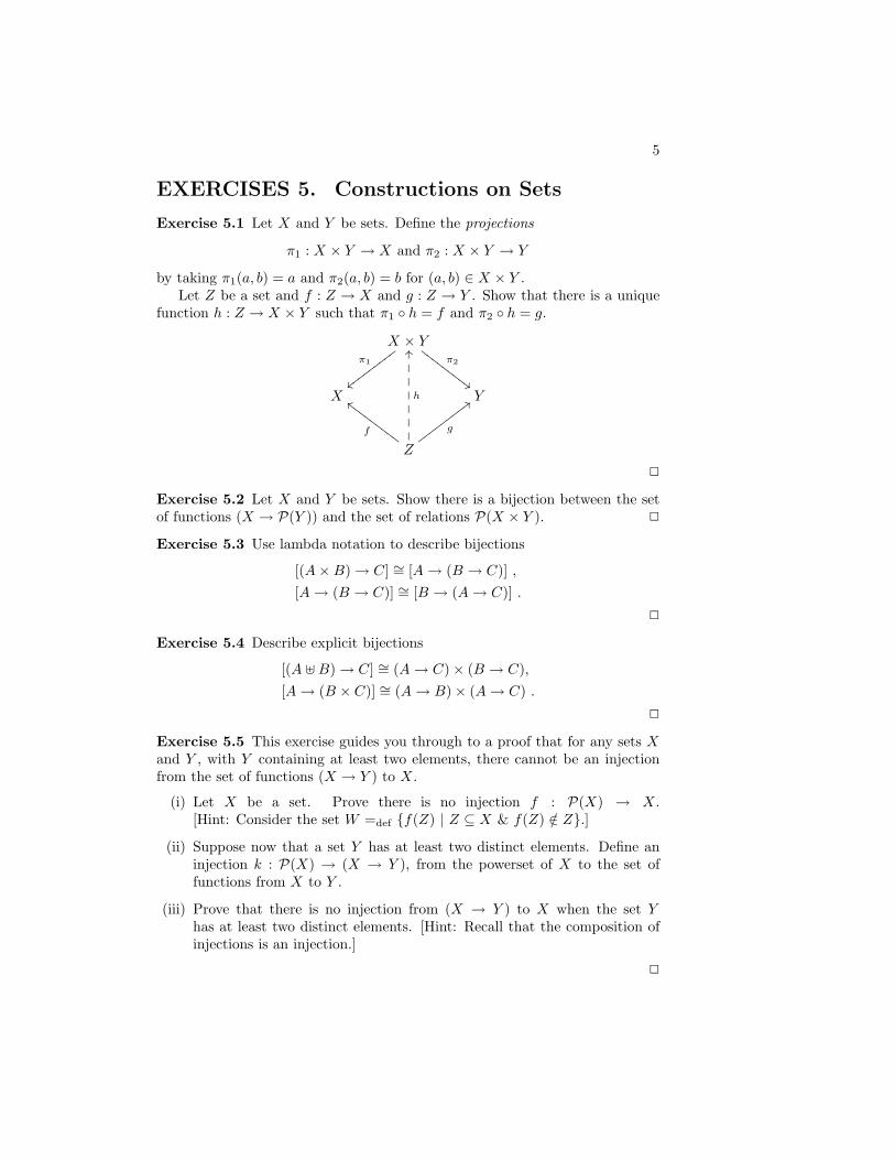
5
EXERCISES 5. Constructions on Sets
Exercise 5.1 Let X and Y be sets. Define the projections
π1 : X × Y → X and π2 : X × Y → Y
by taking π1(a, b) = a and π2(a, b) = b for (a, b) ∈ X × Y .Let Z be a set and f : Z → X and g : Z → Y . Show that there is a unique
function h : Z → X × Y such that π1 ◦ h = f and π2 ◦ h = g.
X × Yπ1
{{wwwwwwwwwπ2
##GGGGGGGGG
X Y
Z
f
ccGGGGGGGGG
h
OO������� g
;;wwwwwwwww
2
Exercise 5.2 Let X and Y be sets. Show there is a bijection between the setof functions (X → P(Y )) and the set of relations P(X × Y ). 2
Exercise 5.3 Use lambda notation to describe bijections
[(A×B)→ C] ∼= [A→ (B → C)] ,[A→ (B → C)] ∼= [B → (A→ C)] .
2
Exercise 5.4 Describe explicit bijections
[(A ]B)→ C] ∼= (A→ C)× (B → C),[A→ (B × C)] ∼= (A→ B)× (A→ C) .
2
Exercise 5.5 This exercise guides you through to a proof that for any sets Xand Y , with Y containing at least two elements, there cannot be an injectionfrom the set of functions (X → Y ) to X.
(i) Let X be a set. Prove there is no injection f : P(X) → X.[Hint: Consider the set W =def {f(Z) | Z ⊆ X & f(Z) /∈ Z}.]
(ii) Suppose now that a set Y has at least two distinct elements. Define aninjection k : P(X) → (X → Y ), from the powerset of X to the set offunctions from X to Y .
(iii) Prove that there is no injection from (X → Y ) to X when the set Yhas at least two distinct elements. [Hint: Recall that the composition ofinjections is an injection.]
2
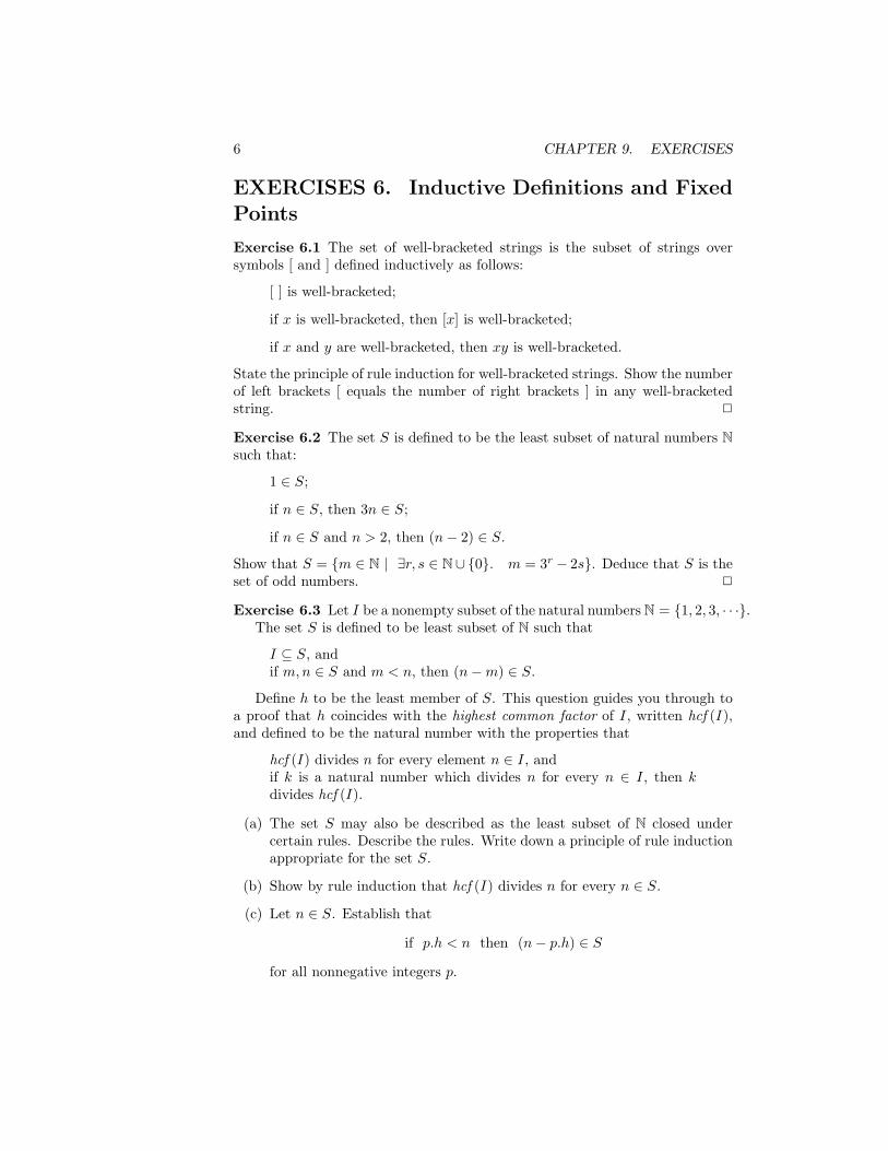
6 CHAPTER 9. EXERCISES
EXERCISES 6. Inductive Definitions and FixedPoints
Exercise 6.1 The set of well-bracketed strings is the subset of strings oversymbols [ and ] defined inductively as follows:
[ ] is well-bracketed;
if x is well-bracketed, then [x] is well-bracketed;
if x and y are well-bracketed, then xy is well-bracketed.
State the principle of rule induction for well-bracketed strings. Show the numberof left brackets [ equals the number of right brackets ] in any well-bracketedstring. 2
Exercise 6.2 The set S is defined to be the least subset of natural numbers Nsuch that:
1 ∈ S;
if n ∈ S, then 3n ∈ S;
if n ∈ S and n > 2, then (n− 2) ∈ S.
Show that S = {m ∈ N | ∃r, s ∈ N∪ {0}. m = 3r − 2s}. Deduce that S is theset of odd numbers. 2
Exercise 6.3 Let I be a nonempty subset of the natural numbers N = {1, 2, 3, · · ·}.The set S is defined to be least subset of N such that
I ⊆ S, andif m,n ∈ S and m < n, then (n−m) ∈ S.
Define h to be the least member of S. This question guides you through toa proof that h coincides with the highest common factor of I, written hcf (I ),and defined to be the natural number with the properties that
hcf (I) divides n for every element n ∈ I, andif k is a natural number which divides n for every n ∈ I, then kdivides hcf (I).
(a) The set S may also be described as the least subset of N closed undercertain rules. Describe the rules. Write down a principle of rule inductionappropriate for the set S.
(b) Show by rule induction that hcf (I ) divides n for every n ∈ S.
(c) Let n ∈ S. Establish that
if p.h < n then (n− p.h) ∈ S
for all nonnegative integers p.
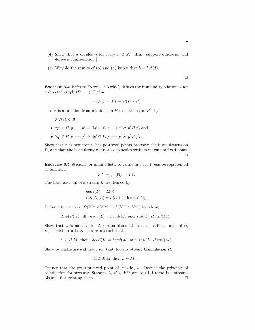
7
(d) Show that h divides n for every n ∈ S. [Hint: suppose otherwise andderive a contradiction.]
(e) Why do the results of (b) and (d) imply that h = hcf (I).
2
Exercise 6.4 Refer to Exercise 3.3 which defines the bisimilarity relation ∼ fora directed graph (P,−→). Define
ϕ : P(P × P )→ P(P × P )
—so ϕ is a function from relations on P to relations on P—by:
p ϕ(R) q iff
• ∀p′ ∈ P. p −→ p′ ⇒ ∃q′ ∈ P. q −→ q′ & p′Rq′, and
• ∀q′ ∈ P. q −→ q′ ⇒ ∃p′ ∈ P. p −→ p′ & p′Rq′.
Show that ϕ is monotonic, has postfixed points precisely the bisimulations onP , and that the bisimilarity relation ∼ coincides with its maximum fixed point.
2
Exercise 6.5 Streams, or infinite lists, of values in a set V can be representedas functions
V∞ =def (N0 → V ) .
The head and tail of a stream L are defined by
head(L) = L(0)tail(L)(n) = L(n+ 1) for n ∈ N0 .
Define a function ϕ : P(V∞ × V∞)→ P(V∞ × V∞) by taking
L ϕ(R) M iff head(L) = head(M) and tail(L) R tail(M) .
Show that ϕ is monotonic. A stream-bisimulation is a postfixed point of ϕ,i.e. a relation R between streams such that
If L R M then head(L) = head(M) and tail(L) R tail(M) .
Show by mathematical induction that, for any stream bisimulation R,
if L R M then L = M .
Deduce that the greatest fixed point of ϕ is idV∞ . Deduce the principle ofcoinduction for streams: Streams L,M ∈ V∞ are equal if there is a stream-bisimulation relating them. 2
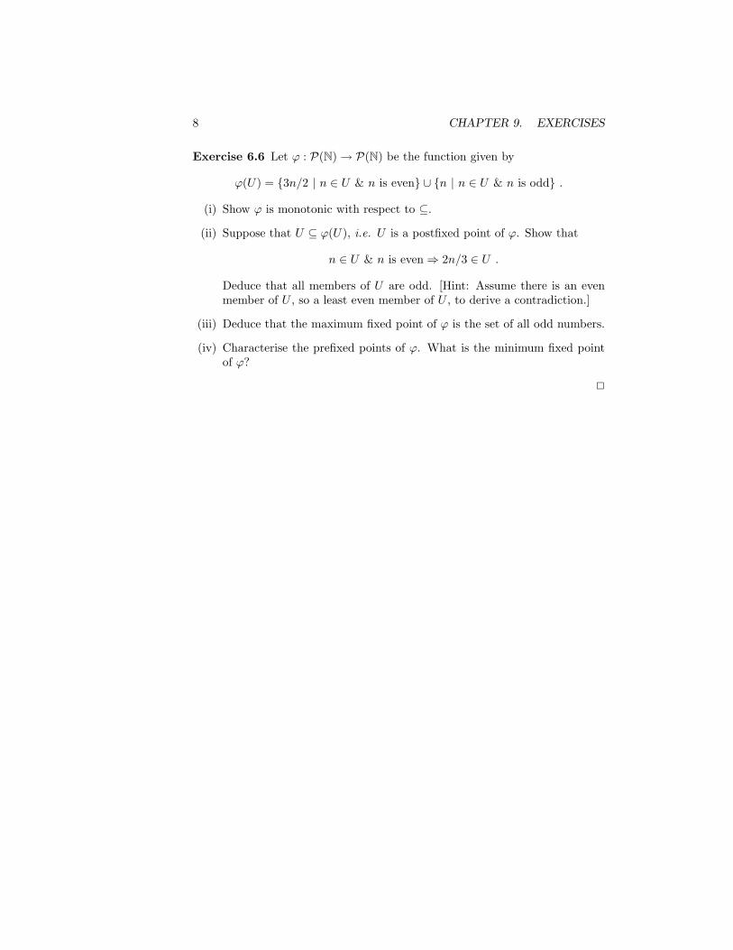
8 CHAPTER 9. EXERCISES
Exercise 6.6 Let ϕ : P(N)→ P(N) be the function given by
ϕ(U) = {3n/2 | n ∈ U & n is even} ∪ {n | n ∈ U & n is odd} .
(i) Show ϕ is monotonic with respect to ⊆.
(ii) Suppose that U ⊆ ϕ(U), i.e. U is a postfixed point of ϕ. Show that
n ∈ U & n is even⇒ 2n/3 ∈ U .
Deduce that all members of U are odd. [Hint: Assume there is an evenmember of U , so a least even member of U , to derive a contradiction.]
(iii) Deduce that the maximum fixed point of ϕ is the set of all odd numbers.
(iv) Characterise the prefixed points of ϕ. What is the minimum fixed pointof ϕ?
2
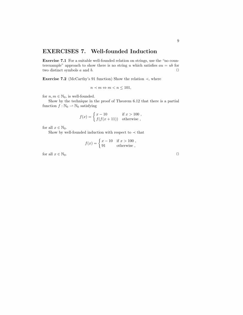
9
EXERCISES 7. Well-founded Induction
Exercise 7.1 For a suitable well-founded relation on strings, use the “no coun-terexample” approach to show there is no string u which satisfies au = ub fortwo distinct symbols a and b. 2
Exercise 7.2 (McCarthy’s 91 function) Show the relation ≺, where
n ≺ m⇔ m < n ≤ 101,
for n,m ∈ N0, is well-founded.Show by the technique in the proof of Theorem 6.12 that there is a partial
function f : N0 ⇀ N0 satisfying
f(x) ={x− 10 if x > 100 ,f(f(x+ 11)) otherwise ,
for all x ∈ N0.Show by well-founded induction with respect to ≺ that
f(x) ={x− 10 if x > 100 ,91 otherwise ,
for all x ∈ N0. 2
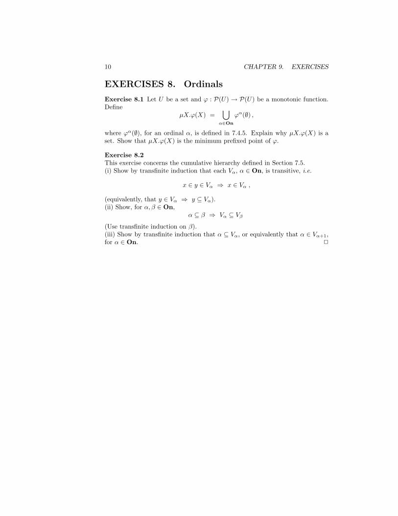
10 CHAPTER 9. EXERCISES
EXERCISES 8. Ordinals
Exercise 8.1 Let U be a set and ϕ : P(U) → P(U) be a monotonic function.Define
µX.ϕ(X) =⋃
α∈On
ϕα(∅) ,
where ϕα(∅), for an ordinal α, is defined in 7.4.5. Explain why µX.ϕ(X) is aset. Show that µX.ϕ(X) is the minimum prefixed point of ϕ.
Exercise 8.2This exercise concerns the cumulative hierarchy defined in Section 7.5.(i) Show by transfinite induction that each Vα, α ∈ On, is transitive, i.e.
x ∈ y ∈ Vα ⇒ x ∈ Vα ,
(equivalently, that y ∈ Vα ⇒ y ⊆ Vα).(ii) Show, for α, β ∈ On,
α ⊆ β ⇒ Vα ⊆ Vβ(Use transfinite induction on β).(iii) Show by transfinite induction that α ⊆ Vα, or equivalently that α ∈ Vα+1,for α ∈ On. 2