Session 8, Unit 15 ISC-PRIME and AERMOD. ISC-PRIME General info. PRIME - Plume Rise Model...
34
Session 8, Unit 15 ISC-PRIME and AERMOD
-
Upload
martha-neal -
Category
Documents
-
view
219 -
download
1
Transcript of Session 8, Unit 15 ISC-PRIME and AERMOD. ISC-PRIME General info. PRIME - Plume Rise Model...

Session 8, Unit 15
ISC-PRIME and AERMOD

ISC-PRIME
General info. PRIME - Plume Rise Model Enhancements Purpose - Enhance ISCST3 by addressing
ISCST3’s deficiency in building downwash Development work funded by Electric Power
Research Institute (EPRI) in 1992 Algorithm developed, codified, and
incorporated into ISCST3 by Earth Tech, Inc. The combined computer program is called ISC-PRIME

ISC-PRIMEDeficiency of ISC3 model Reported over predictions under light wind, stable
conditions Discontinuities in the vertical, alongwind, and
crosswind directions Assumption that the source is always collocated
with the structure causing down washing Streamline flow over a structure is not taken into
account Plume rise is not adjusted due to the velocity deficit
in the wake or due to vertical wind speed shear Concentrations in the cavity region are not linked to
material capture

ISC-PRIMEThe features that ISC-PRIME has and ISCST3 does not: Stack location with respect to building Influence of streamline deflection on plume
trajectory Effect of wind angle on wake structure Effects of plume buoyancy and vertical wind
speed shear on plume rise near building Concentration in near wake (cavity)
ISC-PRIME
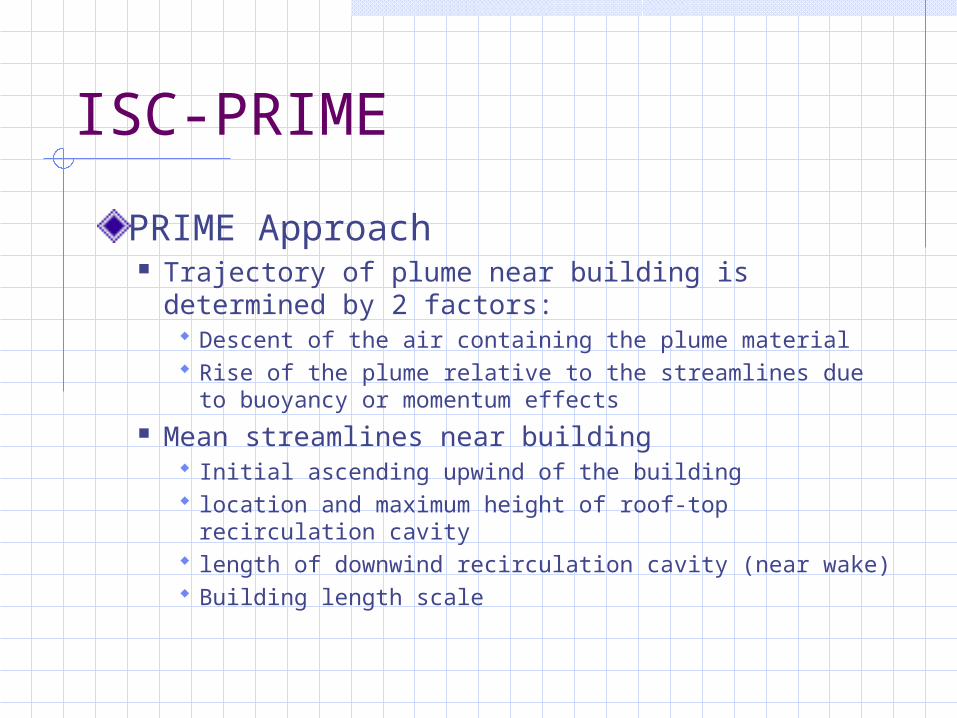
PRIME Approach Trajectory of plume near building is determined
by 2 factors: Descent of the air containing the plume material Rise of the plume relative to the streamlines due to
buoyancy or momentum effects Mean streamlines near building
Initial ascending upwind of the building location and maximum height of roof-top recirculation
cavity length of downwind recirculation cavity (near wake) Building length scale

ISC-PRIME
Running ISC-PRIME Same way to run ISCST3 with exception of
the following three additional keyword in the “SO” pathway: BUILDLEN - projected length of the building along
the flow XBADJ - along-flow distance from the stack to the
center of the upwind face of the projected building YBADJ - across-flow distance from the stack to the
center of the upwind face of the projected building BPIP is modified (called BPIP-PRIME) to
produce these parameters

ISC-PRIME
Independent evaluation by ENSR Evaluation was based on 14 studies
8 tracer studies 3 long-term studies 3 wind tunnel studies

ISC-PRIME
Evaluation results: ISC-PRIME is generally unbiased or
conservative (overpredicting) Statistically ISC-PRIME performs better
than ISCST3 Under stable conditions, ISCST3 is too
conservative and ISC-PRIME is much better Under neutral conditions, the two models
are comparable and ISC-PRIME is slightly better.

ISC-PRIME
Results of evaluation by EPA When no building data is included in the models,
ISCST3 and ISC-PRIME produce the same results ISC-PRIME tend to be less conservative than
ISCST3, but more conservative than observed values
The results of the two model converge beyond 1 km, and become practically the same after 10 km
Generally agree with ENSR’s evaluation and consider the objectives of PRIME have been met

AERMOD
AERMIC – American Meteorological Society/Environmental Protection Agency Regulatory Model Improvement CommitteeAERMOD – AMS/EPA Regulatory ModelGoals of AERMOD – To replace ISC3 (AERMOD has not incorporated the dry and wet deposition features of ISC3)AERMOD is still a steady-state model, but a more sophisticated one than ISC3

AERMOD
New or improved algorithms: Dispersion in both the convective and stable
boundary layers (separate procedures are used for CBL and SBL)
Plume rise and buoyancy Plume penetration into elevated inversions Computation of vertical profiles of wind,
turbulence, and temperature The urban boundary layer The treatment of receptors on all types of
terrain from the surface up to and above the plume height.

AERMOD
AERMOD is a modeling system consisting of: AERMOD - AERMIC Dispersion Model AERMAP – AERMOD Terrain
Preprocessor AERMET - AERMOD Meteorological
Preprocessor

AERMOD
Data flow in AERMOD system

AERMOD
AERMET Use met measurements to compute PBL
parameters Monin-Obukhov Length, L Surface friction velocity, u*
Surface roughness length, z0 Surface heat flux, H Convective scaling velocity, w* Convective and mechanical mixed layer heights,
zic and zim, respectively

AERMOD
Met interface Compute vertical profiles of:
Wind direction Wind speed Temperature Vertical potential temperature gradient Vertical turbulence (w) Horizontal turbulence (v)
Unlike ISC3, both w and v have more than 1 component
Express inhomogeneous parameters in PBL as effective homogeneous values

AERMOD
AERMAP

AERMOD
Treatment of terrain No distinction between simple terrain
and complex terrain Plume either impacts the terrain
or/and follows the flow

AERMOD

AERMOD

AERMOD
Calculation of concentrations Simulate 5 plume types
Direct (real source at the stack) Indirect (imaginary source above CBL to
account for slow downward dispersion) Penetrated (the portion of the plume that
has penetrated into the stable layer) Injected Stable.

AERMOD For CBL, contributions from 3 types of plume
For SBL, similar to ISC3

AERMOD
Dispersion coefficients Contributed by three factors:
ambient turbulence Turbulence induced by a plume buoyancy Enhancements from building wake effects
Plume riseSource characterization Added feature – irregularly shaped area
sources
Adjustment for urban boundary layer For nighttime only

AERMOD
Evaluation Scientifically AERMOD has an advantage
over ISC3 Performance evaluation:
Data: 4 short-term tracer study 6 conventional long-term monitoring
Results (after minor revisions): Nearly unbiased Generally better than ISCST3
Recommended for regulatory applications (rule proposed)

Session 8, Unit 16
CALPUFF

CALPUFF
ISC3, AERMOD Steady-sate Plume Local-scale
CALPUFF Non-steady-state Puff Long-range (up to
hundreds of kilometers)
Can simulate ISC3

CALPUFF
Recommended by IWAQMIWAQM – Interagency Workgroup on Air Quality Modeling EPA U.S. Forest Service National Park Service U.S. Fish and Wildlife Service

CALPUFF
CALPUFF System
CALMET
CALPUFF
CALPOST
Prepare meteorological fields. It generates hourly wind and temperature fields on a 3-D gridded modeling domain.
A Gaussian puff dispersion model with chemical removal, wet & dry deposition, complex terrain algorithm, building downwash, plume fumigation, and other effects
Postprocessing programs for the output fields of met data, concentrations, deposition fluxes, and visibility data

CALPUFF
CALMET process Step 1 – Initial guess wind field is
adjusted for kinematic effects of terrain, slope flows, terrain blocking effects
Step 2 – Introduce observational data into Step 1 wind field to produce final wind field

CALPUFF
CALMET data requirements Surface met data (wind, temp,
precipitation, etc.) Upper air data (e.g., observed vertical
profiles of wind, temp, etc.) Overwater observed data (optional) Geophysical data (e.g., terrain, land
use, etc.)

CALPUFF
Example CALMET wind field
400 420 440 460 480 500 520 540 560 580
U T M E astin g (k m )
4 ,1 30
4 ,1 50
4 ,1 70
4 ,1 90
4 ,2 10
4 ,2 30
UT
M N
orth
ing
(km
)

CALPUFFCALPUFF concept and solutions Plume is treated as series of puffs
Snapshot approach Sampling time – time interval between snapshots Concentrations at receptors are determined at the
snapshot time. One receptors may receive contributions from more than 1 puff
Puffs may move and evolve in size between snapshots Separation between puffs: <1-2 . Otherwise, results are
not accurate Problems – too many puffs (e.g., thousands puffs/hr) Solutions
1. Radially symmetric puffs, OR 2. Non-circular puff (slug)

CALPUFF
Other CALPUFF features Dispersion (dispersion coefficients, buoyancy-
induced dispersion, puff splitting, etc.) Building downwash Plume rise Overwater and coastal dispersion Complex terrain Dry and wet deposition Chemical reaction Visibility modeling Odor modeling
Graphic User Interface (GUI)

CALPUFF
CALPUFF data and computer requirements Up to 16 input files (control, met, geophysical,
source, etc.) Up to 9 output files Computer requirements:
Memory: typical case – 32 MB; more for more sources Computing time: for a 500 MHz PC, 218 sources and
425 receptors 9 hours for CALMET 95 hours for CALPUFF

CALPUFF
Summary Primarily for long range modeling, but
can be used for local modeling A puff model Non-steady state Very sophisticated Resource intensive