Session 4 -5: The benchmark of theoretical gravity models _Theoretical... · The theoretical...
43
Dr. Witada Anukoonwattaka Trade and Investment Division, ESCAP [email protected] ARTNeT- GIZ Capacity Building Workshop on Introduction to Gravity Modelling: 19-21 April 2016, Ulaanbaatar Session 4-5: The benchmark of theoretical gravity models
Transcript of Session 4 -5: The benchmark of theoretical gravity models _Theoretical... · The theoretical...

Dr. Witada Anukoonwattaka
Trade and Investment Division, ESCAP
ARTNeT- GIZ Capacity Building Workshop on Introduction to Gravity Modelling: 19-21 April 2016, Ulaanbaatar
Session 4-5: The benchmark of theoretical gravity models
2
Overview of the workshop
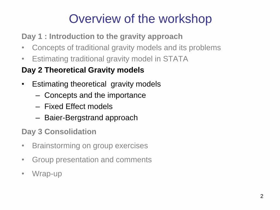
Day 1 : Introduction to the gravity approach
• Concepts of traditional gravity models and its problems
• Estimating traditional gravity model in STATA
Day 2 Theoretical Gravity models
• Estimating theoretical gravity models
– Concepts and the importance
– Fixed Effect models
– Baier-Bergstrand approach
Day 3 Consolidation
• Brainstorming on group exercises
• Group presentation and comments
• Wrap-up
Introduction
• The basic gravity model provides a
respectable place to start.
• But if we look more closely, we will find
that it has some unattractive implications
from an economic point of view.
• Doing some theory allows us to
reformulate the gravity model in much
more attractive way.

• Yesterday, we interpreted b3 = -1 as indicating that a 1%
increase in bilateral distance (trade cost) is associated
with a 1% decrease in bilateral trade.
• In fact, this presents some serious problems in the
context of a world with many countries.
• Do trade flows between i and j only depend on bilateral
trade costs, without any adjustment for the level of trade
costs prevailing on other routes?
ijijjiij etbYbYbbX ....)ln()ln()ln(ln 3210

5
Major weaknesses of the basic gravity:
The basic gravity model cannot handle the facts that:
1. Trade costs of the third party can affect trade between the
two partners.
2. Relative trade costs (relative prices, to be exact) matter, not
absolute trade costs
A consequence:
• The OLS basic gravity models encounter the omitted
variables bias
Ex. trade creation and trade diversion are not captured by the
basic gravity model.
ijijjiij etbYbYbbX )ln()ln()ln(ln 3210

The theoretical gravity model
• A number of papers try to lay theoretical foundations to
gravity model
• For the starting point, we will focus on Anderson &Van
Wincoop (AvW),2003. “The gravity with gravitas”.
• There are several theoretical gravity models developed
for particular purposes.
– Ex. Helpman et.al. (2008), Chaney (2008).
– Showing complex empirical issues that OLS cannot handle
– Sources such as the gravity course on Ben Shepherd’s website
at http://www.developing-trade.com/ provide rich details.

AvW (2003)
• The most formal benchmark for theoretical
gravity model so far
– Bringing the gravity model a step closer to GE effects
– Accounting for “relative price effects” on trade flow
Things affecting “relative price” can influence
bilateral trade flow. No matter the “things” happen
between the two trading partners or happen with third
parties.

Building gravity on micro-foundation
• Consumers have love of variety preferences
with CES structure
• Producers are under monopolistic competition
• Introducing trade costs, and related domestic
and foreign prices
• Closing the model with macroeconomic
accounting identities

AvW (2003) empirical model
kY
k
ijX
k
iY
Sector-k exports from country i to j
World income from sector k
k
jE
k
ij
Exporting country’s income from sector k
Importing country’s expenditure on sector k
Sector-k trade costs between country i and country j

Outward multi-lateral resistance (MTR): looking from export sides
Inward multi-lateral resistance (MTR): looking from import side
Exports from country i to j
depend on trade costs across
ALL possible export markets.
Imports of country j from
country i depend on trade costs
across ALL possible suppliers.
AvW (2003) empirical model
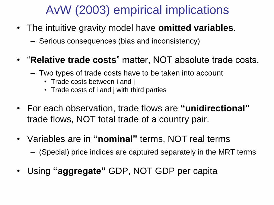
AvW (2003) empirical implications
• The intuitive gravity model have omitted variables.
– Serious consequences (bias and inconsistency)
• “Relative trade costs” matter, NOT absolute trade costs,
– Two types of trade costs have to be taken into account • Trade costs between i and j
• Trade costs of i and j with third parties
• For each observation, trade flows are “unidirectional”
trade flows, NOT total trade of a country pair.
• Variables are in “nominal” terms, NOT real terms
– (Special) price indices are captured separately in the MRT terms
• Using “aggregate” GDP, NOT GDP per capita

AvW (2003) empirical implications
• Need the estimated “trade costs”, NOT just
distance in gravity models.
– The base line can be
– Policy-related variables can be augmented into the
trade cost functions.
• is NOT purely trade cost elasticity, but
combined with elasticity of substitution (k)
b̂
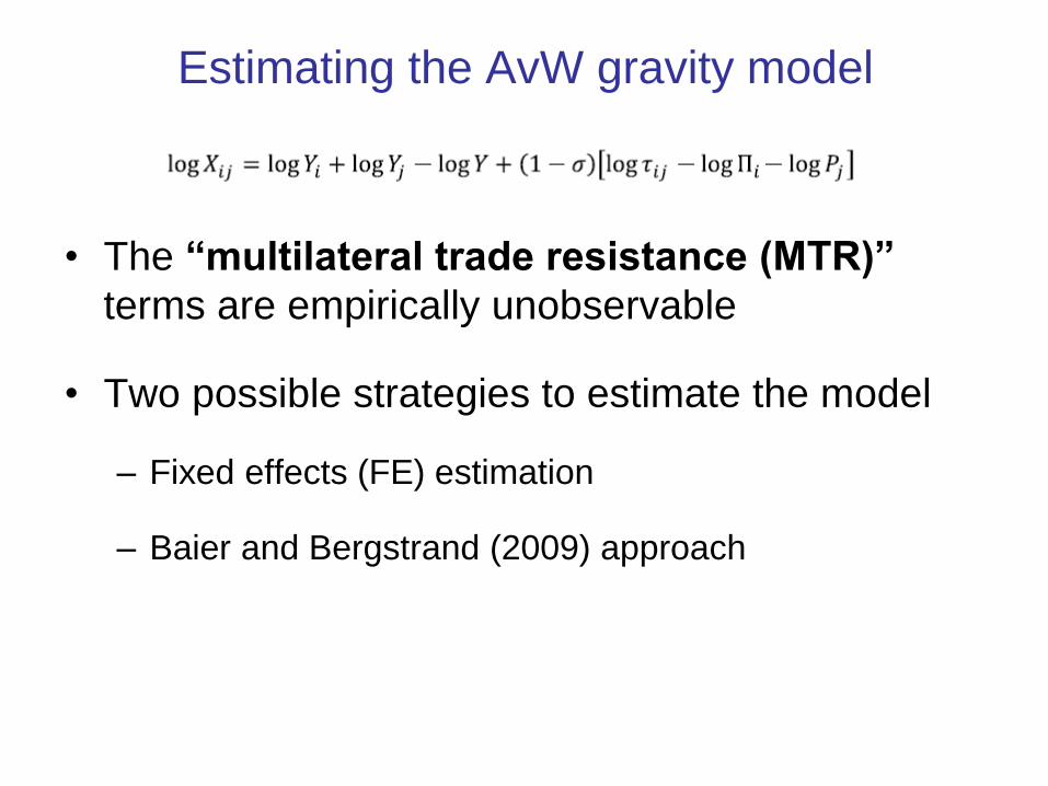
Estimating the AvW gravity model
• The “multilateral trade resistance (MTR)”
terms are empirically unobservable
• Two possible strategies to estimate the model
– Fixed effects (FE) estimation
– Baier and Bergstrand (2009) approach
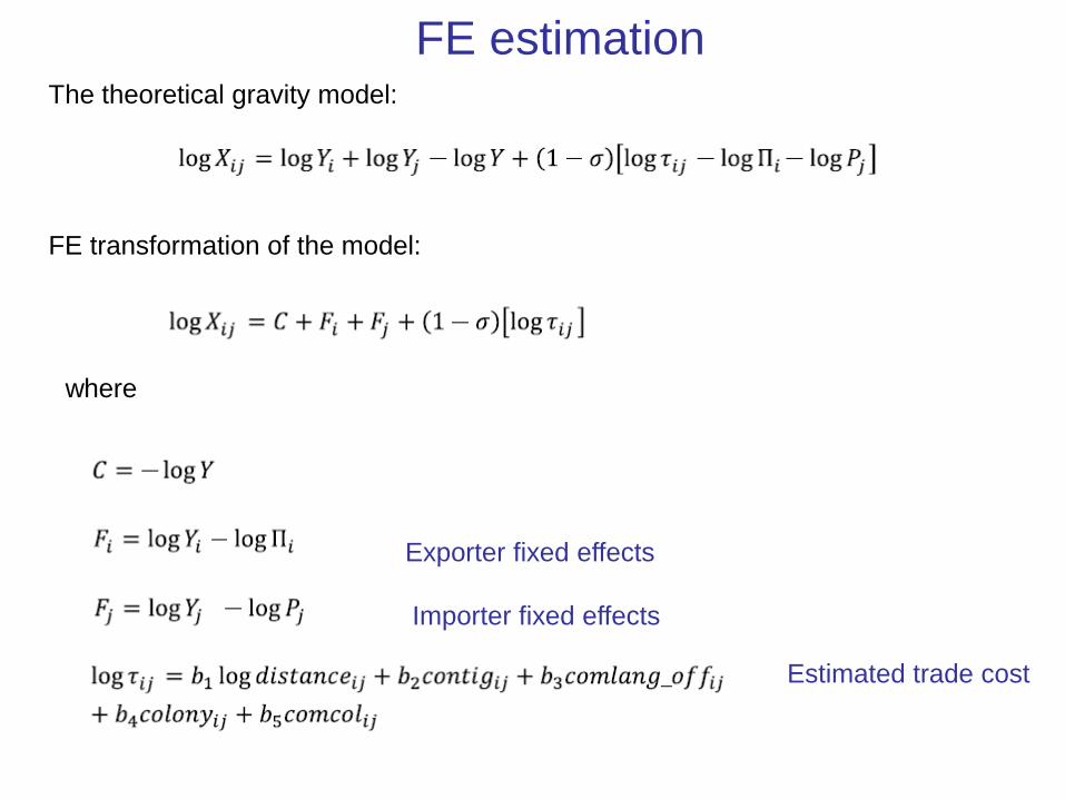
FE estimation The theoretical gravity model:
FE transformation of the model:
where
Exporter fixed effects
Importer fixed effects
Estimated trade cost
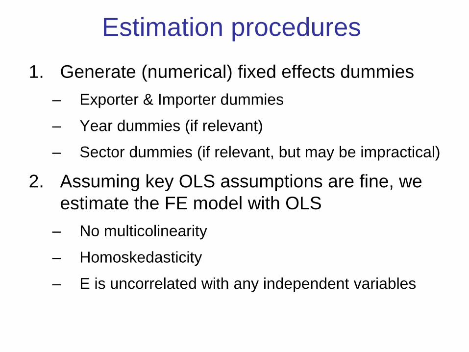
Estimation procedures
1. Generate (numerical) fixed effects dummies
– Exporter & Importer dummies
– Year dummies (if relevant)
– Sector dummies (if relevant, but may be impractical)
2. Assuming key OLS assumptions are fine, we
estimate the FE model with OLS
– No multicolinearity
– Homoskedasticity
– E is uncorrelated with any independent variables

Estimation procedures
3. Variables that vary in the same dimensions as the
FEs CANNOT be included in the model
• Having multicolinearity problems with FEs
• ex. MFN tariffs, ETCR scores
• MUST be transformed into a new variable that vary
bilaterally before including in the model,
• or using alternative approaches.
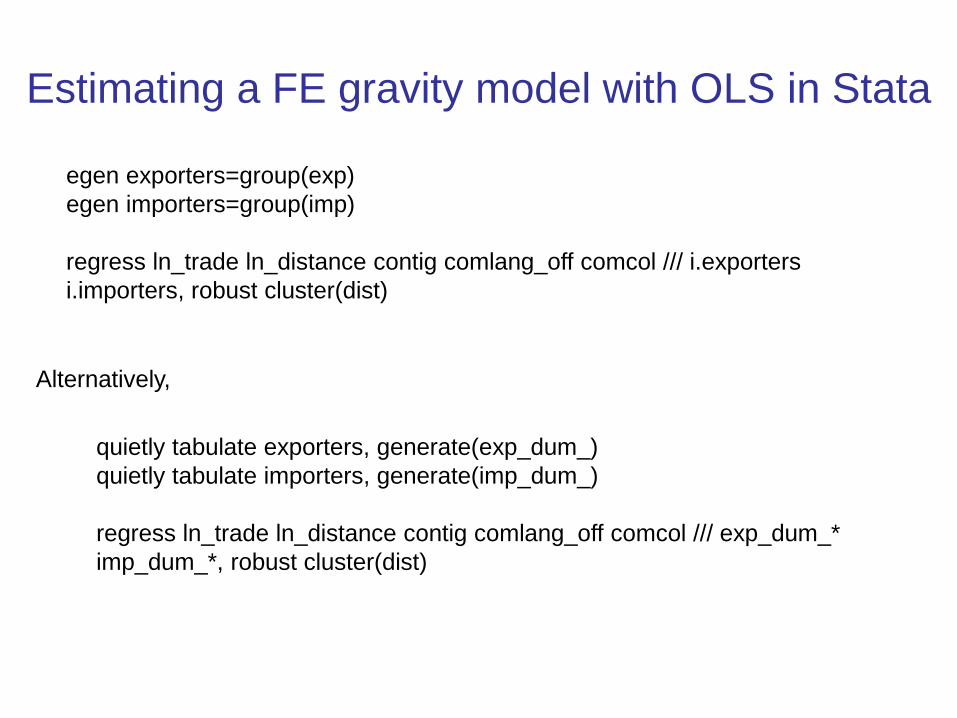
Estimating a FE gravity model with OLS in Stata
Alternatively,
egen exporters=group(exp)
egen importers=group(imp)
regress ln_trade ln_distance contig comlang_off comcol /// i.exporters
i.importers, robust cluster(dist)
quietly tabulate exporters, generate(exp_dum_)
quietly tabulate importers, generate(imp_dum_)
regress ln_trade ln_distance contig comlang_off comcol /// exp_dum_*
imp_dum_*, robust cluster(dist)

Taking account of MTR
• How serious is this OV bias empirically?
quietly regress ln_trade ln_gdp_exp ln_gdp_imp ln_distance contig comlang_off
estimates store Basic
quietly regress ln_trade ln_distance contig comlang_off comcol i.exporters i.importers
estimates store FE
suest Basic FE, robust cluster(dist)
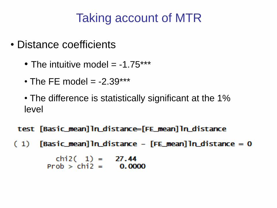
Taking account of MTR
• Distance coefficients
• The intuitive model = -1.75***
• The FE model = -2.39***
• The difference is statistically significant at the 1%
level
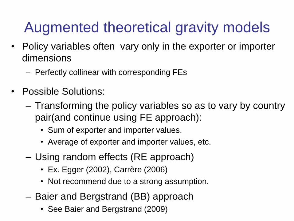
Augmented theoretical gravity models
• Policy variables often vary only in the exporter or importer
dimensions
– Perfectly collinear with corresponding FEs
• Possible Solutions:
– Transforming the policy variables so as to vary by country
pair(and continue using FE approach):
• Sum of exporter and importer values.
• Average of exporter and importer values, etc.
– Using random effects (RE approach)
• Ex. Egger (2002), Carrère (2006)
• Not recommend due to a strong assumption.
– Baier and Bergstrand (BB) approach
• See Baier and Bergstrand (2009)

An augmented FE model gen tariff_sim_both = (tariff_exp_sim+tariff_imp_sim)/2
regress ln_trade tariff_sim_both ln_distance contig comlang_off
comcol i.exporters i.importers, robust cluster(dist)

Dummies and Fixed Effects in STATA
• Option 1: enter the dummies manually and use OLS: egen exporters=group(exp)
egen importers=group(imp)
regress ln_trade tariff_sim_both ln_distance contig comlang_off comcol ///
i.exporters i.importers, robust cluster(dist)
• Option 2: use a panel estimator (OLS + a trick) to
account for one set of dummies: xtset exporters
xtreg ln_trade tariff_sim_both ln_distance contig comlang_off comcol ///
i.importers, robust fe
With the same clustering specification, results should be identical between
regress with dummy variables and xtreg, fe

Note:
• xtreg can only include fixed effects in one dimension. For
additional dimensions, enter the dummies manually.
• For FE with more than 1 dimension:
reghdfe --estimation of a Linear Regression Model
with multiple dimensional Fixed Effects
ivreg2hdfe-- estimation of a linear IV regression
model with two high dimensional fixed effects.

Trade potential in Gravity
25
Identifying “trade potential”
• The OLS estimates give the prediction of
“average” trade level.
• Actually, some countries trade “more” than
average, while others trade “less” than
average.
• Some of the literature uses the sign and
size of the error term to examine trade
potential.

26
• Estimating trade potential
Fist step: estimate the model to get estimated coefficients
Second step: Use estimated coefficients give predicted Xij
Third: Trade potential is the gap between predicted and
actual Xij
ijijjiij etbYbYbbX ....)ln()ln()ln(ln 3210
...)ln(ˆ)ln(ˆ)ln(ˆˆˆln 3210 ijjiij tbYbYbbX
Identifying “trade potential”

27
qui regress regress ln_trade ln_tariff_imp_sim ln_gdp_exp ln_gdp_imp
ln_distance /// comlang_off comcol, robust cluster(dist)
predict ln_tradehat
gen tradehat = exp(ln_tradehat) gen tradeerror = trade-tradehat
list tradeerror exp_name imp_name if exp=="MNG" & tradeerror ~=.
28
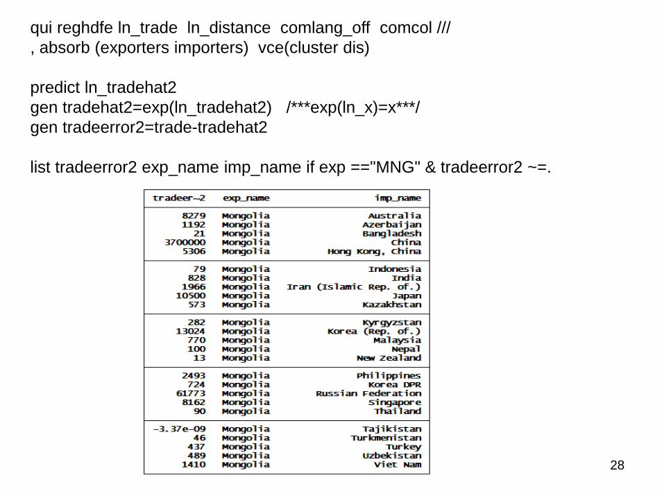
qui reghdfe ln_trade ln_distance comlang_off comcol ///
, absorb (exporters importers) vce(cluster dis)
predict ln_tradehat2
gen tradehat2=exp(ln_tradehat2) /***exp(ln_x)=x***/
gen tradeerror2=trade-tradehat2
list tradeerror2 exp_name imp_name if exp =="MNG" & tradeerror2 ~=.

29
Identifying “trade potential” • Actual Trade- Predicted trade << 0 (Large negative errors:
– A country could be trading more based on their economic and geographical fundamentals
– Something is holding back trade.
• Positive errors: ??
• Keep in mind
– Junk-in, Junk-out
– The error term include also statistical noise and measurement error.
– Do not overemphasized trade potential estimated by gravity model.
– It may just give a first idea of what is going on with particular trade relationships. Things need to work in details of what is holding back trade.

Issues about FEs

Sectoral gravity models
• Dummy variables need to be specified in the importer-
sector, exporter-sector, and sector dimensions, because:
• In addition, trade costs need to be interacted with sector
dummies in order to take account of varying elasticities
of substitution across sectors.

• Depending on the level of sectoral
disaggregation used, this approach can result in
huge numbers of parameters.
• Models can take a long time, and a big
computer, to estimate.
• It is usually much easier to estimate separate
models for each sector.
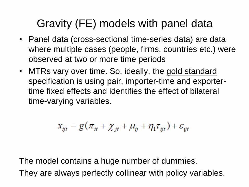
Gravity (FE) models with panel data
• Panel data (cross-sectional time-series data) are data
where multiple cases (people, firms, countries etc.) were
observed at two or more time periods
• MTRs vary over time. So, ideally, the gold standard
specification is using pair, importer-time and exporter-
time fixed effects and identifies the effect of bilateral
time-varying variables.
The model contains a huge number of dummies.
They are always perfectly collinear with policy variables.

Disadvantages of the FE approach
• Losing insights on interested policy impacts
• Dimensionality constraints
• A large number of dummies if running a sectoral
gravity model: Dummies for sectors, exporter-sector,
and importer-sector.
• A larger number of dummies if they are time-variant
• A trick: reduce dimensions by estimating separate
models for each (major) dimension.

Dealing with policy variables

Baier and Bergstrand (BB) Approach
• Taking account of MTR without using dummies
• (Policy) variables that varies by exporter or
importer can be directly included
• Doing a 1st order Taylor series approximation of
the MTR terms.
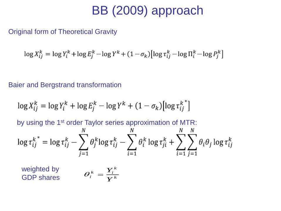
BB (2009) approach
Original form of Theoretical Gravity
Baier and Bergstrand transformation
by using the 1st order Taylor series approximation of MTR:
weighted by
GDP shares k
k
ik
iY
Y
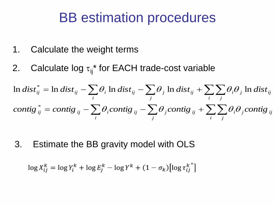
BB estimation procedures
1. Calculate the weight terms
2. Calculate log ij* for EACH trade-cost variable
ijj
i j
iij
j
jij
i
iijij
ijj
i j
iij
j
jij
i
iijij
contigcontigcontigcontigcontig
distdistdistdistdist
*
* lnlnlnlnln
3. Estimate the BB gravity model with OLS

Points to keep in mind
• Need to apply the Taylor approximation to ALL
variables in the trade cost function
• Possible endogeneity problems when using GDP
weights
– BB (2009) recommend using simple averages rather
than the GDP-weighted averages

BB with simple averages in Stata
k
i
k
iN
1Find the weight term:
Calculate log ij*
egen temp1 = mean(ln_distance), by (exp sector)
egen temp2 = mean(ln_distance), by (imp sector)
egen temp3 = sum(ln_distance), by (sector)
gen ln_distance_star = ln_distance - temp1 - temp2 + (1/(58*58))*temp3

BB with simple averages in Stata
A simplified BB model
Note: we assume, for brevity, distance is the only trade cost variable.
A simplified FE model
Reference
• Empirical examples uses the Uncomtrade
dataset on bilateral trade in goods downloaded
from WITS. The original trade data has been re-
aggregated and compiled by to include GDP
data are from the WDIs. Geographical data are
from CEPII. Tariff data are from UNCTAD’s
TRAINS database downloaded from WITS).
• The completed lists of references are provided
in the reading list

Thank you!
Training materials of this
session are drawn largely
from Ben Shepherd (2012).
Available at
http://www.unescap.org/tid/pu
blication/tipub2645.asp