Session 1: Solid State Physics Classical vs. …ee.sharif.edu/~sarvari/25772/PSSD001.pdfClassical...
57
Classical vs. Quantum Mechanics Session 1: Solid State Physics 1
Transcript of Session 1: Solid State Physics Classical vs. …ee.sharif.edu/~sarvari/25772/PSSD001.pdfClassical...

Classical vs. Quantum
Mechanics
Session 1: Solid State Physics
1

1. Intro
2. Birth of QM
3. Schrod. Eq
4. Simple Prob.
Outline
� Introduction� History
� Thomson’s atomic model
� Rutherford’s atomic model
� Birth of QM� Black body radiation
� Photoelectric effect
� Bohr model
� Uncertainty principle
� Double slit
� Schrodinger Equation� Probability density
� Operators
� Postulates of QM
� Simple problems� free electron / particle in box / potential wall / tunneling / Kronig-Penning
problem / Harmonic oscillator
2

1. Intro
2. Birth of QM
3. Schrod. Eq
4. Simple Prob.
History of Chemistry
3
In fourth century B.C., ancient Greeks proposed that matter consisted of fundamental particles called atoms. Over the next two millennia, major advances in chemistry were achieved by alchemists. Their major goal was to convert certain elements into others by a process called transmutation.
Relation of the four ELEMENTS and the four qualities
air fire
water earth
dry
hot
wet
cold
In 400 B.C. the Greeks tried to understand matter (chemicals) and broke them down into earth, wind, fire, and air.

1. Intro
2. Birth of QM
3. Schrod. Eq
4. Simple Prob.
History of Chemistry
4
Serious experimental efforts to identify the elements began in the eighteenth century with
the work of Lavoisier, Priestley, and other chemists. By the end of the nineteenth century, about 80 of the elements had been correctly identified,
The law of definite proportions was correctly interpreted by the
English chemist John Dalton as evidence for the existence of atoms. Dalton argued that if we assume that carbon and oxygen are
composed of atoms whose masses are in the ratio 3:4 and if CO is
the result of an exact pairing of these atoms (one atom of C paired
with each atom of O),
John Dalton (1766–1844)Teacher of James Joule
H --
-- -- -- C N O -- --
-- -- -- -- P S Cl --
-- -- -- Ti -- Cr Mn Fe Co Ni Cu Zn -- -- As -- -- --
-- -- -- -- -- Mo -- -- -- -- Ag -- -- Sn Sb Te -- --
-- -- -- -- -- W -- -- -- Pt Au Hg -- Pb Bi -- -- --
-- -- -- -- -- U
ELEMENTS DISCOVERED BEFORE 1800: (Italicized if discovered after 1700)

1. Intro
2. Birth of QM
3. Schrod. Eq
4. Simple Prob.
Thomson’s Atomic Model
5
Proposed about 1900 by Lord Kelvin and strongly supported by Sir Joseph John Thomson,Thomson’s “plum-pudding” model of the atom had the positive charges spread uniformly throughout a sphere the size of the atom, with electrons embedded in the uniform background.
J. J. Thomson (1856 – 1940)Nobel Prize: 1906
Teacher of Ernest Rutherford and 6 other Nobel winners
Father of G. P. Thomson (Nobel 1937)
“There is nothing new to be discovered in physics now. All that remains is more and more precise measurement.”--- Lord Kelvin, 1900
⊝⊝⊝⊝ ⊝⊝⊝⊝⊝
� �� ���� ��

1. Intro
2. Birth of QM
3. Schrod. Eq
4. Simple Prob.
Rutherford’s Atomic Model
6
Rutherford Scattering (1909):The experimental results were not consistent with Thomson’s atomic model.
Ernest Rutherford(1871 –1937)New Zealand-born
father of nuclear physicsNobel Prize in Chemistry (1908)
Rutherford proposed (1911) that an atom has a positively charged core (nucleus) surrounded by the negative electrons

1. Intro
2. Birth of QM
3. Schrod. Eq
4. Simple Prob.
Failing of the Planetary Model
7
From classical E&M theory, an accelerated electric charge radiates energy (electromagnetic radiation) which means total energy must decrease. Radius r must decrease!!
Electron crashes into the nucleus!?
Nucleus
Physics had reached a turning point in 1900 with Planck’s hypothesis of the quantum behavior of radiation.
1. Intro
2. Birth of QM
3. Schrod. Eq
4. Simple Prob.
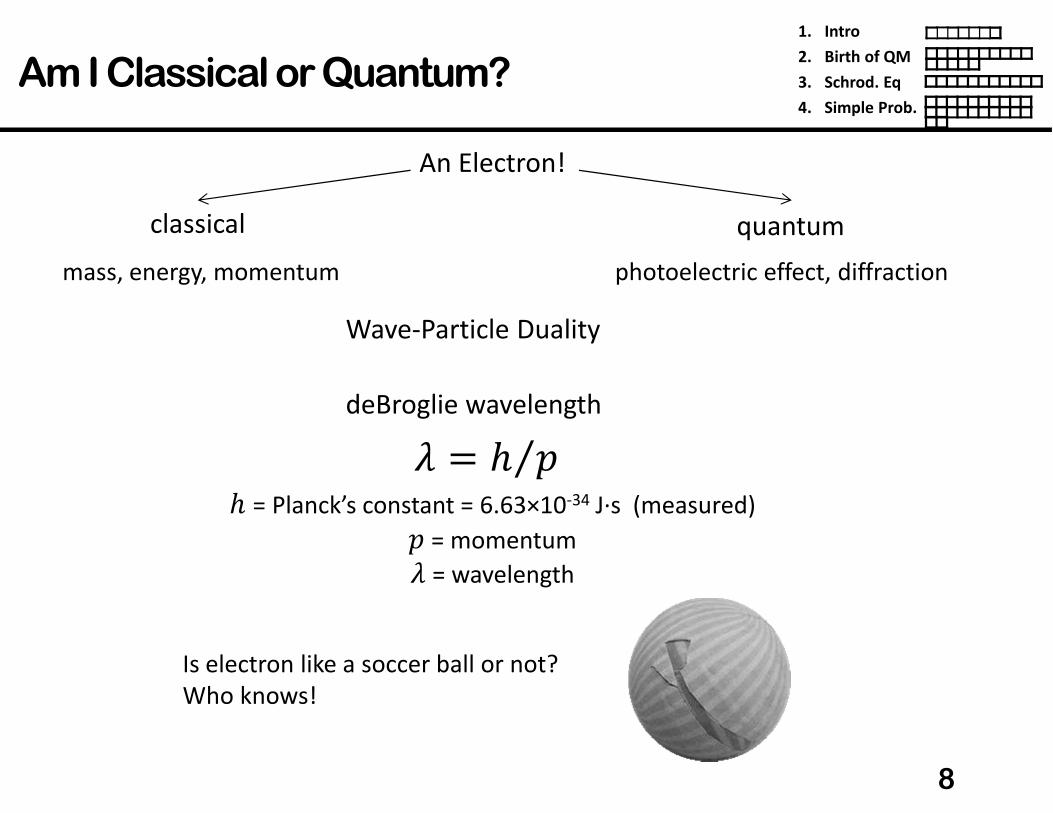
Am I Classical or Quantum?
8
An Electron!
mass, energy, momentum
Wave-Particle Duality
classical quantum
photoelectric effect, diffraction
deBroglie wavelength
� = Planck’s constant = 6.63×10⁻³⁴ J·s (measured)� = momentum� = wavelength
� � � �⁄Is electron like a soccer ball or not?Who knows!

1. Intro
2. Birth of QM
3. Schrod. Eq
4. Simple Prob.
Wave-Particle Duality
9
How do I look?
vs.
� = 6.6×10⁻³⁴ m� = 0.5 J = E/h = 7.5×1032 /s
� �?� = 1Kg � = 1 m/s
� ≅ 1Kg � = 1 m/s
� = 100Kg
� = 6.6×10⁻⁴ m� = 5×10-31 J = 757/s

1. Intro
2. Birth of QM
3. Schrod. Eq
4. Simple Prob.
Black Body Radiation
10
• Temperature is just average energy in each microscopic degree of motion ( (1/2)kT, k = Boltzman’s constant)
• Every object radiates light at its intrinsic frequencies of vibration etc.• A Black Body absorbs all light incident, but must re-radiate light, whose intensity and spectrum depends only upon the temperature.
Classical Mechanics, and Classical EM gave prediction for black body radiation that:1. Disagreed with experiments2. Was logically inconsistent (Infinite total energy).
Planck (1900) found that a very simple formula could be used to calculate the quantum at a particular frequency of EMR � � �
E = energy of the radiation (J)h = Planck’s Constant = 6.63e-34 J·sf = frequency of the EMR (Hz)
Max Planck (1858 – 1947)Nobel Prize (1918)

1. Intro
2. Birth of QM
3. Schrod. Eq
4. Simple Prob.
Photo Electric Effect
11
• Light shining on a metal will liberate electrons,
but the photon energy hf must be greater than a threshold energy (equal to binding energy of electron in metal.)
• The threshold effect is independent of light intensity (energy density of light).• Na requires 2.5eV = Green
In 1905 an unknown physicist
named Albert Einstein came up with an idea that built on what Planck had said.The light consist of particles named
photon.Photon comes from the Greek word for light. Einstein originally called photons a “light quantum.” The chemist Gilbert N. Lewis came up with the name photo.

1. Intro
2. Birth of QM
3. Schrod. Eq
4. Simple Prob.
Fathers of QM!
12
Louis de Broglie (1892 –1987)
Introduced wave-particle duality in hisPhD thesis, 1924Nobel Prize in Physics, 1929
Erwin Schrödinger (1887 –1961)
the Schrödinger equation, January 1926Nobel Prize in Physics, 1933Max Born (1882 –1970)
@ University of Göttingen, he came intocontact with: Klein, Hilbert, Minkowski,Runge, Schwarzschild, and VoigtPhysical interpretation of the Sch ‘s wave functionMatrix mechanicsNobel Prize in Physics, 1954
Werner Heisenberg (1901 –1976)
Student of Summerfeld/BornMatrix mechanics / Uncertainty PrincipleNobel Prize in Physics, 1932
Pascual Jordan (1902 – 1980)
Student of BornMatrix mechanics
Paul Dirac ( 1902 –1984)
Fermi–Dirac statisticsspecial theory of relativity + quantummechanics � ‘quantum field theory’Nobel Prize in Physics, 1933

1. Intro
2. Birth of QM
3. Schrod. Eq
4. Simple Prob.
H2Emission & Absorption Spectra
13
Sun and stars are made of Hydrogen and Helium,
The galaxies are receding from us (redshift)
Balmer Series [Joseph Balmer, 1885]
� � � 12� � 1�� , � � 3, 4, 5, …

1. Intro
2. Birth of QM
3. Schrod. Eq
4. Simple Prob.
Photon Emission
14
“Continuous” spectrum “Quantized” spectrum
Any
Δ�is p
oss
ible
On
ly c
erta
in Δ�a
re a
llow
ed
With Δ� � ��/λIf λ = 440 nm, Δ� = 4.5 x 10⁻¹⁹ J
Emis
sio
n
Ener
gy
Δ�Ener
gy Δ�Ener
gy

1. Intro
2. Birth of QM
3. Schrod. Eq
4. Simple Prob.
Bohr Atomic Model
15
Introduced by Niels Bohr (1885 –1962) in 1913, a Dane, proposed his model of the atom while working at Cambridge University in England
Atom: a small, positively charged nucleus surrounded by electrons that travel in circular orbits around the nucleus (similar to the solar system)

1. Intro
2. Birth of QM
3. Schrod. Eq
4. Simple Prob.
Bohr Atomic Model
16
Bohr’s postulate (1913):(1) An electron in an atom moves in a circular orbit about the nucleus under the influence of the Coulomb attraction between the electron and the nucleus, obeyingthe laws of classical mechanics.(2) An electron move in an orbit for which its orbital angular momentum is � � �� � �� 2 ⁄ , � � 1,2,⋯, � Planck’s constant(3) An electron with constant acceleration moving in an allowed orbit does not radiate electromagnetic energy. Thus, its total energy � remains constant.(4) Electromagnetic radiation is emitted if an electron, initially moving in an orbit of total energy �", discontinuously changes its motion so that it moves in an orbit of total energy �#. The frequency of the emitted radiation is $ � %�" � �#& �⁄ .
Louis de Brogliehis 1924 thesis(1892 –1987)
11 years later !
wave-particle duality � � � �⁄de Broglie standing wave
��' � ���"�# �$ � �" � �#

1. Intro
2. Birth of QM
3. Schrod. Eq
4. Simple Prob.
Bohr’s Model
17
Kinetic energy:
Potential energy:
(�
)(
Total energy:
* � �+ → 14 -. )(�'� � ���'� � ��' � �� / → '0� 4 -. �����)(��0 � ���'0 � 14 -. )(���
1 � �2 )(�4 -.'� 3'456 � � )(�4 -.'
7 � 8���� � )(�4 -.%2'&� � 7 � 1 � �7 ⟹�0 � � �)�(:4 -. � 2�� 1�� � �)� 13.6eV��

1. Intro
2. Birth of QM
3. Schrod. Eq
4. Simple Prob.
Bohr Atomic Model
18
Energy Bands:
wave-particle duality � � � �⁄de Broglie standing wave
��' � ��
�8
���?�:

1. Intro
2. Birth of QM
3. Schrod. Eq
4. Simple Prob.
Bohr’s Model
19
for
$ � �" � �#�� 14 -. ��)�(:4 �? 1�#� � 1�"�1� � $� � �5)� 1�#� � 1�"�
�5 � 14 -. � �(:4 ��? � �@
Ionization above 13.6eV
Lyman Series
Balmer Series
Pashchen Series
n=1
n=2
n=3
n=4n=5

1. Intro
2. Birth of QM
3. Schrod. Eq
4. Simple Prob.
Quantum Mechanics and Real Life!
20
Why chalk is white, metals are shiny?
TunnelingHeisenberg’s uncertainty principleParticle may exist in a superposition stateMeasurement, collapse of the wavefunction
QM arguably the greatest achievement of the twentieth century!QM changed our view of the world/philosophy of life!QM been attacked by many prominent scientist!QM is “non-local”!QM enables quantum computing!QM is bizarre!
For us as Elect. Engineers:+ Solid state technology (Integrated circuits)- Tunneling through gate oxideInformation age is become available by QM!
Colors ← Absorbing transitions ← transition energies ←QM
Blackbody radiation: Quantum statistics of radiation (is using to find temp. of stars)

1. Intro
2. Birth of QM
3. Schrod. Eq
4. Simple Prob.
Uncertainty Principle
21
In quantum world, each particle is described by a wave packet. This wave behavior of the particle is reason behind uncertainty principle.
Adding several waves of different wavelength together will produce an interference pattern which localizes the wave. But the process spreads the momentum and makes it more uncertain.Inherently:
Precisely determined momentumA sine wave of wavelength �, implies that the momentum � is precisely known but the wavefunction is spread over all space.
Δ�ΔA B � 2 ⁄

1. Intro
2. Birth of QM
3. Schrod. Eq
4. Simple Prob.
Diffraction & Uncertainty Principle
22
Uncertainty
Uncertainty principle is a consequence of wave nature of matter
sin F � � G⁄∆I ≅ G/2∆�J ≅ � sin F � %� �⁄ &%� G⁄ &ΔI∆�J � � 2⁄
Heisenberg:
ΔI∆�J � � 2 ⁄
∆I ∆F

1. Intro
2. Birth of QM
3. Schrod. Eq
4. Simple Prob.
Interference –Double Slit
23
Plain wave:
Hence a beam of monoenergetic electrons produces a sinusoidal interference pattern, or “fringes”, on the screen, with the fringes separated by a distance �K � �� 3⁄
L ∝ (4"N.Oassume � ≫ 3Wave on the screen:
Q � R � � A�2� � 3�8�
LKT6UU0 ∝ (4"V W4X �⁄ YZ[Y � (4"V WZX �⁄ YZ[YLKT6UU0 ∝ (4"\ cos R3A2�
where
LKT6UU0 � ∝ cos� 3A�� � 12 1 � cos 2 3A��
Young’s double slits
electron double slits

1. Intro
2. Birth of QM
3. Schrod. Eq
4. Simple Prob.
Double Slit & Quantum Mechanics
24
some bizarre consequences:By blocking 1 slit → interference fringes disappearBy uncovering 1 slit → parts the screen that were bright now become dark
extremely low electron currents (never 2 electrons at given time)→ same interference pattern
Diffractive effects are strong when the wavelength is comparable to the size of an object.• Spacing between the atoms are on the order of Å.• Electron microscope!
�_~0.1nm

1. Intro
2. Birth of QM
3. Schrod. Eq
4. Simple Prob.
Schrodinger Equation
25
Electron can behave like plane wave with � � � �⁄ wave equation Ψ � d("�eW f⁄Simplest choice: Helmholtz wave equation for monochromatic wave
time-independent Schrodinger equation
g�Ψ � �R�Ψ where R � 2 �⁄ � � �⁄���g�Ψ � ��Ψ
� ��2�. g�Ψ � ��2�.Ψ → ��2�. � K.E.=Total energy(�) − Potential energy(1)
� ��2�. g�Ψ � � � 1%'& Ψ� ��2�. g� � 1%'& Ψ � �Ψ� ��2�. g� � 1%'& Ψ � �Ψ
Note: we have not “derived” Schrödinger’s equation. Schrödinger’s equation has to be postulated, just like Newton’s laws of motion were originally postulated. The only justification for making such a postulate is that it works!

1. Intro
2. Birth of QM
3. Schrod. Eq
4. Simple Prob.
Schrodinger Equation
26
time-dependent Schrodinger equation
� � �.��: � ���� � �.�� 1 � ����2�.��: �⋯
and
�$ � �h � 1 � ��R�2�. 3Ψ3i � �jhΨΨ%A, i& � d(4"%kl4VW&� ��2�.
3�Ψ3A� � 1%'&Ψ � j� 3Ψ3i� ��2�.3�Ψ3A� � 1%'&Ψ � j� 3Ψ3i
� � �.�� � 1 � ��2�. � 1 � ��R�2�.
3�Ψ3A� � �R�Ψ
1. Intro
2. Birth of QM
3. Schrod. Eq
4. Simple Prob.
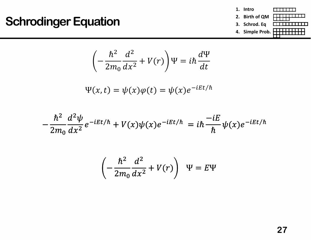
Schrodinger Equation
27
� ��2�.3�3A� � 1%'& Ψ � j� 3Ψ3i
Ψ A, i � L%A&Q%i& � L%A&(4"ml �⁄
� ��2�.3�L3A� (4"ml �⁄ � 1%A&L%A&(4"ml �⁄ � j��j�� L%A&(4"ml �⁄� ��2�.3�L3A� (4"ml �⁄ � 1%A&L%A&(4"ml �⁄ � j��j�� L%A&(4"ml �⁄
� ��2�.3�3A� � 1%'& Ψ � �Ψ� ��2�.3�3A� � 1%'& Ψ � �Ψ

1. Intro
2. Birth of QM
3. Schrod. Eq
4. Simple Prob.
Probability Density
28
Physical interpretation of the wavefunctionn%'& �probability of finding a particle at ' ∝ L ' �Most likely at A, never can be found at C!If we find it at B, what does it mean?
2 L ' �3?' � 1
A%i& � 2A L A, i �3A
A B C
L%A& L∗%A&Measurement will change the wave function! The value of L is not measurable. However, all measurable quantities of a particle can be derived from L.
It is meaningless to talk about the position of the particle, as a wave function describes it, but we can find the expected value for the position, ⟨A⟩.
r%i& � 2L∗ A, i rsL A, i 3A

1. Intro
2. Birth of QM
3. Schrod. Eq
4. Simple Prob.
Operator
29
A%i& � t A L A, i �3A Show that:3 A3i � � j��2L∗ uLuA 3AMomentum operator:
general operator:
v � 2Ψ∗vwΨ3A3I3x
� � �� � �3 A3i � �j�2L∗ uLuA 3A � 2L∗ �j� uuA L 3A

1. Intro
2. Birth of QM
3. Schrod. Eq
4. Simple Prob.
Postulates of Quantum Mechanics
30
3D wave-function: Ψ%A, I, x; i& , Ψ%Oz; i& , L%Oz&1D wave-function: Ψ%A; i&window of QM to the real world Ψ∗%A; i& Ψ%A; i&Dynamical variables:position, momentum, energy
33AΨ%A, i&
Classical: Quantum:
Operator
We have seen operators before
operator
operand

1. Intro
2. Birth of QM
3. Schrod. Eq
4. Simple Prob.
Postulate 1:
31
The state of a system is described by a wave function of the coordinates and the timeΨ%Oz; i& , (which is often complex-valued) the complete wavefunction depends on coordinates O and time i.Ψ∗%A; i& Ψ A; i 3{ is the probability that the system is in the volumeelement 3{ at time i.
Example: The wavefunction of the plane monochromatic light
Thus Ψ and uΨ/u%A, I, x&must be:
wave-particle duality
(1)Single-value; (2) Continuous; (3) Quadratically integrable
L � d(�e"%Wf4|l&� � ��, � � � �⁄
L � d(�ef "%W}~4ml&

1. Intro
2. Birth of QM
3. Schrod. Eq
4. Simple Prob.
Postulate 2:
32
The motion of a nonrelativistic particle is governed by the Schrödinger equation��Ψ � � ��2�.3�3A� � 1%'& Ψ � j� 3Ψ3i
Ψ A, i � L%A&Q%i& � L%A&(4"ml �⁄time-dependent Schrodinger equation
� ��2�.3�L3A� � 1%'&L � �L� ��2�.3�L3A� � 1%'&L � �L
time-independent Schrodinger equation
If L8, L�, … , L0are the possible states of a microscopic system, then the linear combination of these states is also a possible state of the system
Ψ ���"L""Ψ ���"L""In classical systems: we often use linear equations as a first approximation to nonlinear behaviorIn quantum mechanics: The linearity of the equations with respect to the quantum mechanical amplitude is not an approximation of any kind. this linearity allows the full use of linear algebra for the mathematics of quantum mechanics.

1. Intro
2. Birth of QM
3. Schrod. Eq
4. Simple Prob.
Postulate 3:
33
For every classical observable there is a corresponding linear hermitian quantum mechanical operator.
Classical operator Quantum operator
Position, A A� � AMomentum(x), �W �̂W � �j� uuA%�W& %�̂W&
Kinetic Energy, 7 � }Y�� 7� � �̂�2�Potential Energy, 1 1w � 1
Energy , � � 7 � 1(Schrödinger eq.) �� � j� uui
v � 2Ψ∗vwΨ3A3I3x

1. Intro
2. Birth of QM
3. Schrod. Eq
4. Simple Prob.
Pauli Exclusion Principle
34
Every atomic or molecular orbital can only contain a maximum of two electrons with opposite spins.

1. Intro
2. Birth of QM
3. Schrod. Eq
4. Simple Prob.
Solvay
35

1. Intro
2. Birth of QM
3. Schrod. Eq
4. Simple Prob.
Simple Problems
36
Free electron (metals)
Harmonic oscillator (acoustic vibration � phonon,Emag waves � photon)
Particle in a box (quantum well, optoelectronic)Ideal (infinite) wellFinite well
Potential wall (transmission, reflection)
Tunneling (Tunneling diode, STM)
Kronig-Penning problem (Solid state, Bandgap)

1. Intro
2. Birth of QM
3. Schrod. Eq
4. Simple Prob.
Free Electron
37
Free electron 1 A � 0, with energy �� ��2�.
3�L3A� � 1%'&L � �L� ��2�.3�L3A� � 1%'&L � �L time-independent Schrodinger equation
3�L3A� � �2�.��� L � �R�L3�L3A� � �2�.��� L � �R�LL � dZ(4"VW � d4(Z"VWL � dZ(4"VW � d4(Z"VW R � 2�.��R � 2�.�� � � ��R�2�.� � ��R�2�.Ψ%A, i& � dZ(4"%VW4kl& � d4(Z"%VW4kl&Ψ%A, i& � dZ(4"%VW4kl& � d4(Z"%VW4kl& �
R

1. Intro
2. Birth of QM
3. Schrod. Eq
4. Simple Prob.
Effective Mass
38
� � ��R�2�. → �∗ � ��3�� 3R�⁄� � ��R�2�. → �∗ � ��3�� 3R�⁄�
R
� �
RR
�( �j �+d�

1. Intro
2. Birth of QM
3. Schrod. Eq
4. Simple Prob.
1-D Quantum Well (Box)
39
Outside the box:
Consider a particle with mass m under potential as:
3�L3A� � 2���� L � 03�L3A� � 2���� L � 0
2 L∗L3AZ545 � 2 d� sin 0eW[ �3A[
. � 1 → d � 2 �⁄2 L∗L3AZ545 � 2 d� sin 0eW[ �3A[
. � 1 → d � 2 �⁄
R � 2�� �⁄R � 2�� �⁄
� � � 2��� → �0 � �� ���2���� � � 2��� → �0 � �� ���2���L 0 � L � � 0 → L � d sin RA ; R � � � , � � 1,2,3,⋯L 0 � L � � 0 → L � d sin RA ; R � � � , � � 1,2,3,⋯
1%A&1%A&1 � ∞1 � ∞ 1 � ∞1 � ∞1 � 01 � 01 � ∞ → L � 01 � ∞ → L � 0
Inside the box:
assin RA , cos RAsin RA , cos RAcontinuity of L at 0 and �: � is the quantum number
normalization:
L0 � �[ sin%0e[ W&
L8L8L�L�L?L?
00 ��

1. Intro
2. Birth of QM
3. Schrod. Eq
4. Simple Prob.
1-D Quantum Well (Box)
40
�8�8
1 � ∞1 � ∞ 1 � ∞1 � ∞1 � 01 � 0
L0 � �[ sin%0e[ W&
L�L�
L?L?
L8L8�� � 4�8�� � 4�8�� � 9�8�� � 9�8
��� 2���⁄00 ��
�0 � �� ���2���
� ↗ ∞ →free electron

1. Intro
2. Birth of QM
3. Schrod. Eq
4. Simple Prob.
Eigenvalue -Eigenfunction
41
Solutions:with a specific set of allowed values of a parameter (here energy), eigenvalues �0 (eigenenergies) and with a particular function solution associated with each such value, eigenfunctions L0It is possible to have more than one eigenfunction with a given eigenvalue, a phenomenon known as degeneracy.
even function / odd function
Note:It is quite possible for solutions of quantum mechanical problems not to have either odd or even behavior, e.g., if the potential was not itself symmetric.When the potential is symmetric, odd and even behavior is very common.Definite parity is useful since it makes certain integrals vanish exactly.
�8�8
1 � ∞1 � ∞ 1 � ∞1 � ∞1 � 01 � 0
L�L�
L?L?
L8L8 �� � 4�8�� � 4�8�� � 9�8�� � 9�8
��� 2���⁄00 ��

1. Intro
2. Birth of QM
3. Schrod. Eq
4. Simple Prob.
Quantum Behavior
42
Only discrete values of that energy possible, with specific wave functions associated with each such value of energy. This is the first truly “quantum” behavior we have seen with “quantum” steps in energy between the different allowed states.
Differences from the classical case:1 - only a discrete set of possible values for the energy2 - a minimum possible energy for the particle,above the energy of the classical "bottom" of the box,E8 � ��� 2���⁄sometimes called a "zero point" energy (ground state).3 - the particle is not uniformly distributed over the box, (almost never found very near to the walls of the box)the probability obeys a standing wave pattern.In the lowest state (n =1), it is most likely to be found near the center of the box. In higher states, there are points inside the box, where the particle will never be found. Note that each successively higher energy state has one more “zero” in the eigenfunction. this is very common behavior in quantum mechanics.
�8�8
1 � ∞1 � ∞ 1 � ∞1 � ∞1 � 01 � 0
L�L�
L?L?
L8L8 �� � 4�8�� � 4�8�� � 9�8�� � 9�8 ��� 2���⁄00 ���~0.5��%atom&�8 � 1.5(1�� � �8 � 4.5(1

1. Intro
2. Birth of QM
3. Schrod. Eq
4. Simple Prob.
Sets of Eigen functions
43
completeness of sets of eigenfunctions.
Familiar case: Fourier series
Similarly for every A , 0 � A � �:
we can express any function between positions A � 0and A � �as an expansion in the eigenfunctions of this quantum mechanical problem.Note that there are many other sets of functions that are also complete.
A set of functions such as the L0 that can be used to represent a function such as the %A& is referred to as a “basis set of functions” or simply, a “basis”.The set of coefficients (amplitudes) �0 is then the “representation” of %A&in the basis L0. Because of the completeness of the set of basis functions L0 , this representation is just as good a one as the set of the amplitudes at every point A between 0 and �.
i � �+0 sin%0el� &50�8 A � � +0 sin%0eW[ &5
0�8 � ��0L0%A&50�8
as L0 � Y� sin%��� W& hence �0 � �Y+0

1. Intro
2. Birth of QM
3. Schrod. Eq
4. Simple Prob.
Sets of Eigen functions
44
In addition to being “complete,” the set of functions L0%A& are “orthogonal”.
Definition: Two functions �%A& and �%A& are orthogonal if
Definition: Kronecker delta
A set of functions that is both normalized and mutually orthogonal, is said to be“orthonormal”.
Orthonormal sets are very convenient mathematically, so most basis sets are chosen to be orthonormal. Note that orthogonality of different eigenfunctions is very common in quantum mechanics, and is not restricted to this specific example where the eigenfunctions are sine waves.
2 �∗ A � A 3A[. � 0
��0 � �0, � � �1, � � �2 L0∗ A L� A 3A[. � ��0
A �� �0L0 A0 → �� � 2L0∗ A A 3A

1. Intro
2. Birth of QM
3. Schrod. Eq
4. Simple Prob.
1-D Finite Well
45
We first need to find the values of the energy for which there are solutions to the Schrödinger equation, then deduce the corresponding wavefunctions.Boundary conditions are given by continuity of the wavefunction and its first derivative.
3�L3A� � �2���� L � �R�L3�L3A� � �2���� L � �R�L
1%A&1%A&1 � �1 � � 1 � �1 � �1 � 01 � 0
assume � � �
Finite L:L�� � * sin RA � � cos RA
00 ���� ���� ������
Region ��Region ��
R � 2���R � 2���
Region � and ���Region � and ���3�L3A� � 2�%� � �&�� L � ��L3�L3A� � 2�%� � �&�� L � ��L � � 2�%� � �&�� � 2�%� � �&�⇒ L � d(�W � �(4�W, A � 0andA ¡ �
⇒ ¢L� � d(�W, A � 0L��� � �(4�W, A � �

1. Intro
2. Birth of QM
3. Schrod. Eq
4. Simple Prob.
1-D Finite Well
46
for � � � : (1) Quantization of energies. (2) Particle almost bounded In the well.for � ¡ � : all energies are possible. (plane wave)
1%A&1%A&1 � �1 � � 1 � �1 � �1 � 01 � 0
00 ���� ���� ������£L� � d(�W, A � 0L�� � * sin RA � � cos RA ,L��� � �(4�W, A � � 0 � A � �
L� � L�� @A � 03L�3A � 3L��3A @A � 0L�� � L��� @A � �3L��3A � 3L���3A @A � �2 L A �3A545 � 1
⟹d�*�� → �
L L �

1. Intro
2. Birth of QM
3. Schrod. Eq
4. Simple Prob.
Finite vs. Infinite Well
47
0.39��0.39��n=1
n=2
n=3
n=4
n=5
n=6
2.47 eV
9.87 eV
22.2 eV
39.5 eV
61.7 eV
88.8 eV
0.39��0.39��n=1
n=2
n=3
n=4
n=5
n=6
1.95 eV
7.76 eV
17.4 eV
30.5 eV
63.6 eV
46.7 eV
64 eV

1. Intro
2. Birth of QM
3. Schrod. Eq
4. Simple Prob.
Potential Well
48
1%A&1%A&1 � 1.1 � 1.00 AA�� ����
���2� 3�L�3A� � �L����2� 3�L�3A� � �L�
B.C. � d, �, ¥
Region ��Region ��
Region �Region �
L� � d("VW � �(4"VW %A � 0&
3�L�3A� � R�L� � 03�L�3A� � R�L� � 0 wherewhere R � 2�� �⁄R � 2�� �⁄���2� 3�L��3A� � 1.L�� � �L�����2� 3�L��3A� � 1.L�� � �L��3�L��3A� � ��L�� � 03�L��3A� � ��L�� � 0 wherewhere � � 2�%� � 1.& �⁄� � 2�%� � 1.& �⁄
L�� � ¦(�W � ¥(4�W%A ¡ 0&Ψ� A, i � d(" VW4ml �⁄ � �(" VWZml �⁄Ψ�� A, i � ¥(4�W4"ml �⁄
¥d � 2� � j 1. � � �1.�d � 2� � 1. � 2j 1. � � �1.� � 1(1, 1. � 2(1→ 8��..�0�penetration depth

1. Intro
2. Birth of QM
3. Schrod. Eq
4. Simple Prob.
Potential Well
49

1. Intro
2. Birth of QM
3. Schrod. Eq
4. Simple Prob.
Tunneling
50
1%A&1%A& ��
00 AA�� �������2� 3�L3A� � �L � �L���2� 3�L3A� � �L � �L
� � 2�%� � �& �⁄� � 2�%� � �& �⁄• Transmission coefficient (T): The probability that the particle penetrates the barrier.
• Reflection coefficient (R): The probability that the particle is reflected by the barrier.
• T + R = 1
��������£ L� � ("VW � '(4"VW %A � 0& L�� � d(�W � �(4�W %0 � A � �& L��� � i("VW %A ¡ �&R � 2�� �⁄R � 2�� �⁄
L� � L�� @A � 0 3L�3A � 3L��3A @A � 0L�� � L��� @A � �3L��3A � 3L���3A @A � �⇒ § d�i ⟶ © � i �' ⟶ � � ' �

1. Intro
2. Birth of QM
3. Schrod. Eq
4. Simple Prob.
Tunneling
51
1%A&1%A& ��
00 AA�� ����
L�� � * sin RA � � cos RA
��������
© � 1 � ��4� � � � sin� �� 48��
©1 classical
quantum
� � 2�%� � �& �⁄� � 2�%� � �& �⁄For � � �For � � � © � 1 � �2 ����� 48For � ≫ �For � ≫ � ©~exp¬�2�� 2�%� � �&

1. Intro
2. Birth of QM
3. Schrod. Eq
4. Simple Prob.
Tunneling
52L�� � * sin RA � � cos RA

1. Intro
2. Birth of QM
3. Schrod. Eq
4. Simple Prob.
Applications of Tunneling
53
Alpha decay:In order for the alpha particle to escape from the nucleus, it must penetrate a barrier whose energy is several times greater than the energy of the nucleus-alpha particle system.
Nuclear fusion:Protons can tunnel through the barrier caused by their mutual electrostatic repulsion.
Scanning tunneling microscope:• The empty space between the tip and the sample surface forms the “barrier”.• The STM allows highly detailed images of surfaces with resolutions comparable to the size of a single atom: 0.2 nm lateral, 0.001nm vertical.

1. Intro
2. Birth of QM
3. Schrod. Eq
4. Simple Prob.
Why Harmonic Oscillator?
54
Mo
lecu
lar
po
ten
tial
en
ergy
Inter-nuclear separation�U
+
-
+
-

1. Intro
2. Birth of QM
3. Schrod. Eq
4. Simple Prob.
Harmonic Oscillator
55
1 A � 8�RA�
A
A particle subject to a restoring force: * � �RA � ��h�AThe potential energy � A � 8�RA� � 8�Rh�A�
The Schrodinger equation ���2� 3�L3A� � 8�Rh�A�L � �L���2� 3�L3A� � 8�Rh�A�L � �LEasy guessL A � �(4®WY → ¦ � �h2� , � � 8��h
This is actually the ground state!
The actual solution:L0 A � �h �⁄ 20�! exp ��h2� A� �0 �h� A
�0 � � � 8� �h, � � 0, 1, 2, …

1. Intro
2. Birth of QM
3. Schrod. Eq
4. Simple Prob.
Harmonic Oscillator?
56
A
�0 � � � 8� �h, � � 0, 1, 2, …
�. � 8��h�8 � ?��h�� � °��h�? � ±��hGround state �. � ²Y�h , ∆� � �h ∆�The blue curves represents probability densities for the first three states
� � 0� � 1
� � 2
The orange curves represents the classical probability densities corresponding to the same energies
As n increases the agreement between the classical and the quantum mechanical results improves.

1. Intro
2. Birth of QM
3. Schrod. Eq
4. Simple Prob.
Linearly Varying Potential
57
�
A
bulk2D channelOxide
Ban
d S
tate
s
�#Quantum confinement
-.-8-�-?-: