AD-A252 517

May 1992 CWIS SERTATION

Finding an H-Function Distribution for the Sum ofIndependent H-Function Variates

Carl Dinsmore Bodenschatz, Captain

- ~ ~ ~ ~ ~ - A! DSIT~L C-

AFIT Student Attending: University of Texas, Austin AFIT/CI/CIA- 92-005D

AFIT/CIWright-Patterson AFB OH 45433-6583

- ... E. -' TA %I LN

Approved for Public Release lAW 190-1Distributed UnlimitedERNEST A. HAYGOOD, Captain, USAFExecutive Officer

IDTIC _______uM rm~

.ELECTEJUL f 192 .1

__~ 9-1800692 7 09 015

233

-.~~~.. .,,~ .....F.. .. ..

FINDING AN H-FUNCTICt DISTRIBUTION

FOR THE SU4 OF INDEPENDENT

H-FUNCTICN VARIATES

by

CARL DINSKORE BODDISCATZ, B.A., H.S.

DISSETATION

Presented to the Faculty of the Graduate School of

The University of Texas at Austin

in Partial Fulfillnmnt

of the Requirements

for the Degree of

DOCTOR OF PHILOSOPHY

THE UNIVERSITY OF TEXAS AT AUSTIN

May 1992

To God,

for the beauty and sirrplicity of the H-function

and for my ability to study it;

To my parents, Carl A. and Jody,

for teaching me the value of knowledge

and instilling in me a cnmitment to quality in

everything I atteapt;

To my wife, Debbie,

for her continued love and friendship,

honesty, pureness of heart, and inner strength;

To my sons, Luke, John, and Paul,

for their future challenges, comitmnnt toexcellence, and coplete fulfillment.

Acoession ForNTIS RA&IDTIC TAB

0Uuannounced 0Just if ication

By: Dlst ribut !on/

__ / Availability Codes

Avail anid/orDiet special

FINDING AN H-FUNCION DISTRIBUTIC

FOR THE SX4 OF INDEPENDENT

H-FUNCTION VARIATES

APPROVED BY

DISSERTATION CO*ITTEE:

esley es

S Paul A . Jen

W. T. Guy, Jr.

0*-Q.,fb-4 4 ''

01 iVeD. -ok, .dt

ID.4 ,Jr.~

Copyright

by

Carl Dinanore Bodenschatz

1992

A(,cNaLEDGEN4TS

I would like to express my sincere admiration, gratitude,

and respect to Dr. J. Wesley Barnes, my supervising professor,

who embodies the perfect combination of theoretical insight,

practicality, intelligence, and cornvn sense. His suggestions

were always correct, timely, and properly measured.

My gratitude extends to Drs. Paul A. Jensen, William T.

Guy, Jr., Olivier Goldscbhidt, and Ivy D. Cook, Jr. for their

contributions as members of my dissertation canittee and as

instructors in my graduate courses. A special note of thanks

is due Dr. Cook for introducing me to the fascinating world of

H-functions and encouraging my continued research in this area.

I also want to thank the other faculty menbers, staff, and

graduate students in the Department of Mechanical Engineering

for their instruction, support, and friendship.

I a grateful to the Department of Mathenatical Sciences

at the U.S. Air Force Academy for sponsoring my doctoral

program. Most importantly, I want to thank my wife, Debbie,

and our sons for their love, understanding, patience, and

support throughout this experience.

C. D. B.

v

FINDING AN H-FUNCTION DISTRIBUTION

FOR THE SUM OF INDEPNIDE T

H-FUNCTION VARIATES

Publication No.

Carl Dinmnore Bodenschatz, Ph.D.The University of Texas at Austin, 1992

Supervisor: J. Wesley Barnes

A practical method of finding an H-function distribution

for the sum of two or more independent H-function variates is

presented. Sirrple formulas exist which imediately give the

probability density function, as an H-fumcticn distribution, of

the random variable defined as the product, quotient, or power

of independent H-function variates. Unfortunately, there are

no similar formulas for the sum or difference of independent H-

function variates.

The new practical technique finds an H-function

distribution whose moments closely Tatch the moments of the

vi

randao variable defined as the sum of independent H-function

variates. This allows an analyst to find the distribution of

more complicated algebraic combinaticns of independent randam

variables. The method and inplementing computer program are

demonstrated through five exarnples. For comparison, the exact

distribution of the general smu of independent Erlang variates

with different scale parameters is derived using Laplace

transforms and partial fractions decomposition.

The H-function is the most general special function,

enccipassing as a special case nearly every named matheatical

function and continuous statistical distribution. The Laplace

and Fourier transforms (and their inverses) and the derivatives

of an H-function are readily-determined H-functions. The

Mellin transform of an H-function is also easily obtained. The

H-function exactly represents the probability density function

and cmarulative distribution function of nearly all continuous

statistical distributions defined over positive values.

A previously unstated restriction on the variable in the

H-function representations of power functions and beta-type

functions is highlighted. Several ways of overcomning this

limitation when representing nathaitical functions are

presented. The restriction, however, is an advantage when

vii

representing certain statistical distributions. Many new H-

function representations of other mathematical functions are

also given.

The hierarchical structure among classes of H-functions is

given through seven new theorens. Every class of H-functions

is wholly contained in mny higher-order classes of H-functions

through the application of the duplication, triplication, and

nultiplication formulas for the gamma function.

Four new theorems show when and how a generalizing

constant my be present in an H-function representation. Many

generalized H-function representations are given, including

those of every cumulative distribution function of an H-

function variate.

viii

TABLE OF COTETS

CIMPTER PAGE

1. INTRODUCTION AND REVIEW ............................... 1

1.1. Purpose and Scope ............................... 1

1.2. Literature Survey ............................... 4

1.3. Integral Transforms and Transform Pairs ......... 8

1.3.1. Laplace Transform ....................... 9

1.3.2. Fourier Transform ....................... 11

1.3.3. Mellin Transform ........................ 12

1.4. Transformations of Independent Random Variables . 13

1.4.1. Distribution of a Sum ................... 15

1.4.1.1. Infinite Divisibility ......... 17

1.4.1.2. Special Cases ................. 17

1.4.1.3. Reproductive Distributions .... 18

1.4.2. Distribution of a Difference ............ 19

1.4.3. Distribution of a Product ............... 20

1.4.4. Distribution of a Quotient .............. 21

1.4.5. Distribution of a Variate to a Power .... 22

1.4.6. Moments of a Distribution ............... 22

ix

C21AP'ER PACE

2. THE H-FUNC1'ION ..................... 24

2.1. Primrary Definition............................. 25

2.- Alternate Definition........................... 27

* 2.3. Sufficient Convergence Conditions ................ 28

2.4. Properties ..................................... 36

2.4.1. Reciprocal of an Argumrent ................ 37

2.4.2. Argument to a Power ..................... 37

2.4.3. Multiplication by the Argument to a Power 38

2.4.4. First Reduction Property ................ 38

2.4.5. Second Reduction Property ................ 39

*2.4.6. Hierarchical Relationships Among

Orders of H-Fumctions ................... 40

*2.4.7. Generalizing Constant ................... 49

2.4.8. Derivative............................. 59

2.4.9. Laplace Transform...................... 61

2.4.10. Fourier Transform ...................... 62

2.4.11. Mellin Transform...................... 63

* 2.5. Special Cases - Mathematical Functions ........... 63

* 2.6. Functions Represented Over a Restricted Range .. 76

*2.7. Mofnents of an H-Function and Infinite Summubility 80

2.8. Evaluation of the H-F'.mction .................... 84

x

CHIAPTER PACE

3. THE H-FUNCTION DISTRIBUTION ........................... 87

3.1. Definition ...................................... 87

3.2. Moments of an H-Function Distribution ........... 88

3.3. Evaluation of the H-FunctionDistribution Constant ........................... 89

* 3.4. Cumulative Distribution Function ................ 91

* 3.5. Special Cases - Statistical Distributions ....... 93

* 3.6. Arbitrary Ranges for Type VI H-Function Variates 109

3.7. Transformrations of IndependentH-Function Variates ............................. 112

3.7.1. Distribution of a Product ............... 113

3.7.2. Distribution of a Quotient .............. 115

3.7.3. Distribution of a Variate to a Power .... 117

* 3.7.4. Use of Jacobs' (B,b) Plot in FindingPowers of First Order H-Function Variates 118

3.7.5. Distribution of a Sum ................... 122

4. FINDING AN H-FUNCTION DISTRIBUTION FOR THE L14 ........ 126

4.1. Moments of the Sum .............................. 129

4.2. H-Function Parameter Estinates .................. 131

4.2.1. Method of Mcments ....................... 132

4.2.2. Reducing the System ofNonlinear Equations ..................... 133

xi

C2MPTER PAGE

4.2.3. Solving the System ofNonlinear Equations ..................... 136

* 4.3. Special Considerations for Type VIH-Functicm Variates ............................. 138

* 4.4. Demonstration of the Technique .................. 141

4.4.1. Example 1 - Sum of Three Independent,Identically Distributed Gamma Variates .. 145

4.4.2. Example 2 - Sum of Two IndependentErlang Variates with Different X ........ 147

4.4.3. Example 3 - Sum of Two IndependentStandard Uniform Variates ............... 148

4.4.4. Exaiple 4 - Sum of Two Independent,Identically Distributed Beta Variates ... 150

4.4.5. Example 5 - Sum of Two IndependentVariates with Weibull and RayleighDistributions ........................... 152

5. COMPARING THE ESTIMATED H-FUNCTION TO THE EXACTDISTRIBUTION OF THE SUM ............................... 154

5.1. Finding the Exact Distribution of the Sun ....... 155

5.1.1. Convolution Integral .................... 156

5.1.2. Reproductive Distributions .............. 163

5.1.3. Erlang Distributions with Different X ... 164

5.2. Measures of Merit ............................... 172

5.2.1. Estimated Sums of Squares of Error ...... 173

5.2.2. Estimated Mean Squared Error ............ 174

xii

CHAPTER PAGE

5.2.3. Maximum Absolute Difference ............. 174

5.2.4. Integrated Absolute Density Difference .. 174

* 5.3. Demmstrated Results ............................ 175

5.3.1. Example 1 - Su of Three Independent,Identically Distributed Gamma Variates .. 175

5.3.2. Example 2 - Sun of Two IndependentErlang Variates with Different X ........ 176

5.3.3. Example 3 - Sum of Two IndependentStandard Uniform Variates ............... 178

5.3.4. Example 4 - Sun of Two Independent,Identically Distributed Beta Variates ... 181

6. QI4CLUSIONS AND RECMEinDATINS FUR FURTHER S=UDY ..... 184

APPENDIX

A. OUTPUT FROM Conn= PROGRAM ......................... 193

B. GRAPHICAL DEPICTIONS OF SUMS OF SELECTED INDEPEDENTUNIFORM, POWER FNCTION, AND BETA VARIATES ............ 220

BIBLIOGRAPHY .............................................. 225

VITA ...................................................... 232

* Indicates the section contains significant new material.

xiii

LIST OF FI(JRES

Figure

1 Venn Diagram of Certain Ccamn Statistical

Distributions as H- 0 and Hi0 H-Function0 1 1 1Distributions ......................................... 108

2 Classical Statistical Distributions as FirstOrder H-Functions in (B,b) Space ...................... 119

3 Graphical Comparison of the H-Function and theExact Distribution of Example 2 ....................... 178

4 Graphical Ccrparison of the H-Function and theExact Distribution of Exanple 3 ....................... 180

5 Graphical Camparison of the H-Function and theExact Distribution of ExaMple 4 ....................... 183

xiv

LIST OF TABLES

Table Page

1 Convergence Types for H-Functions of Eq (2.1) ..... 30

2 Convergence Types f or H-Functions of Eq (2.2).......... 33

3 Maoents of Trigonetric and Hyperbolic Functions ....... 84

xv

CHAPTER 1

INTROW=ICt AND REVIE

1.1. PURPOSE AND SCOPE

The primary purpose of this research effort was to develop

a practical method of finding an H-function distribution for

the sum of two or more independent H-function variates. Simple

formulas exist which immediately give the probability density

function (p.d.f.), as an H-function distribution, of the random

variable defined as the product, quotient, or power of

independent H-function variates. Unfortunately, there are no

similar formulas for the sum or difference of independent H-

function variates.

A related issue was whether the class of H-functions is

closed under the operation of multiplication. In other words,

is the product of two H-functions another H-function? It is

important to nake the distinction here between the product of

two H-functions and the p.d.f. of the random variable defined

as the product of two H-function variates. It is well know

that the latter case is an H-function. But the former case was

unproven. Of course, similar statements can be made about the

1

2

quotient of two H-functions.

If the class of H-functions is closed under

multiplication, one could easily find the p.d.f. (as an H-

function) of the sum or difference of independent H-function

variates. The Laplace (or Fourier) transforms of the H-

function variates in the sum (or difference) are immediately

available as H-functions of higher order. The product of these

H-functions (in transform space) would yield the transform of

the desired density. If this product was available as another

H-function, it could be inverted from transform space

analytically.

Because the H-function can exactly represent nearly every

common mathematical function and statistical density, there was

ample reason to suspect that the product of two H-functions

was, in general, another H-function. Indeed, there are many

cases where two individual functions and their product are all

special cases of the H-function.

Throughout this thesis, a number of other new results are

identified with an asterisk. Sufficient convergence conditions

for the alternate definition of the H-function are given in

Section 2.3. These show how the H-function nay be evaluated by

the sum of residues, without first changing the form of the

alternate definition of the H-function to that of the primary

3

definition.

The hierarchical structure among classes of H-functions is

given through seven new theorems in Section 2.4.6. Every class

of H-functions is wholly contained in mnny higher-order classes

of H-functions through the application of the duplication,

triplication, and multiplication formulas for the gamm

function. Figure 1 in Section 3.5 illustrates this

hierarchical structure with a venn diagramn showing mony commio

statistical distributions as first and second order H-function

distributions.

Four new theorem in Section 2.4.7 show when and how a

generalizing constant nay be present in an H-function

representation. Many generalized H-function representations

are given, including those of every cumulative distribution

function of an H-function variate. The generalizing constant

is also possible in the H-function representations of power

functions, the error function and its conplement, the

incomplete gamma function and its ccmplemunt, the incmplete

beta function and its complement, mny inverse trigonometric

and hyperbolic functions, and the logarithmic functions.

A number of new H-function representations of certain

mathematical functions and statistical distributions are given

in Sections 2.5, 2.6, and 3.6. Several of these expand upon a

4

previously unstated limitation on the variable in the H-

function representations of power functions and beta-type

functions.

The exact distribution of the general sum of independent

Erlang variates with different scale parameters, X, is derived

in Section 5.1.3. An Erlang variate is simply a gamma variate

with an integer shape parameter r. The derivation uses partial

fractions to decaqpose the product of Laplace transforms of the

individual densities. This produces a sum of terms, each of

which can easily be inverted fran transform space, yielding the

desired density of the sum of independent variates.

Since the H-function is not defined for zero or negative

real arguments, the scope of this research effort was limited

to continuous random variables defined only over positive

values. Continuous and doubly infinite distributions such as

the normal and Student's t are only represented as H-functions

in their folded forms.

1.2. LITERATURE SURVEY

Regrettably, little research in the field of H-functions

has been done in the United States. Much of what is known

about the H-function is due to Indian mthemticians. Mathai

and Saxena [1978] and Srivastava et al [1982] compiled many

results of the early study of H-functions. In recent years,

5

Soviet mathematicians [Prudnikov et al, 1990] have shown a

considerable interest in the H-function and have developed

significant new results.

The foundation of H-function theory is grounded in the

gasm function, integral transform theory, complex analysis,

and statistical distribution theory. Therefore, several

landmark references such as Abramowitz and Stegun [1970),

Erd~lyi [1953], Erd~lyi [1954], and Springer [1979], though

somewhat dated, have timeless value.

Carter [1972] defined the H-function distribution and,

using Mellin transform theory, gave startling and powerful

results showing that products, quotients, and rational powers

of independent H-function variates are themselves H-function

variates. Further, the p.d.f. of the new random variable can

inuediately be written as an H-function distribution. The

usual techniques of conditioning on one of the random variables

and/or using the Jacobian of the transformation are no longer

necessary.

The above results become especially useful when one

realizes that nearly every common positive continuous random

variable can be written as an H-function distribution.

Therefore, the p.d.f. of any algebraic combination involving

products, quotients, or powers of any number of independent

6

positive continuous random variables can imiediately be written

as an H-function distribution.

Carter [1972] also wrote a FCRTRAN computer program to

calculate the mments of an algebraic combination of

independent H-function variates and approximate the p.d.f. and

cumulative distribution function (c.d.f.) from these nunents.

The approximation procedure was developed by Hill [1969] and,

if possible, uses either a Grar-Charlier type A series (Hermite

polynomial) or a Laguerre polynomial series. If a series

approxirration is not possible, the first four nmrents are used

to fit a probability distribution from the Pearson family. As

Carter [1972] himelf notes "... there were nany situations in

which the nethods did not work or in which the approxirations

were totally unsatisfactory."

Springer [1979] literally wrote the book on the algebra of

random variables. He gives an excellent explanation of the

value of integral transform in finding the distribution of

algebraic combinations of random variables. He also gave the

known applications of the H-function in these problem.

Cook [1981] gave a very thorough survey and an extensive

bibliography of the literature related to H-functions and H-

function distributions. He also presented a technique for

finding, in tabular form, the p.d.f. and c.d.f. of an algebraic

7

combination (including sum and excluding differences) of

independent H-function variates.

Cook's technique [1981; Cook and Barnes, 1981] first uses

Carter's [1972] results to find the H-function distribution of

any products, quotients, or powers of random variables. The

Laplace transform of each term in the resulting sum of

independent H-function variates is then obtained. These

transform functions are evaluated and multiplied at

corresponding values of the transform variable, yielding a

tabular representation of the Laplace transform in transform

space. This Laplace transform is then numerically inverted

using Crurp's method. His FORTRAN computer program implements

this technique and will plot the resulting p.d.f. and c.d.f.

Bodenschatz and Boedigheimer [1983; Boedigheimer et al,

1984] developed a technique to fit the H-function to a set of

data using the method of moments. The technique can be used to

curve-fit a mathematical function or to estimate the density of

a particular probability distribution. Their FORTRAN coMputer

program will accept known moments, univariate data, ordered

pair data from a relative frequency, or ordered pair data

directly from the function.

Kellogg [1984; Kellogg and Barnes, 1987; Kellogg and

Barnes, 1989] studied the distribution of products, quotients,

8

and powers of dependent random variables with bivariate H-

fumction distributions. Jacobs [1986; Jacobs et al, 1987]

presented a method of obtaining parameter estimates for the H-

function distribution using the method of maximum likelihood or

the method of moments.

Prudnikov et al [1990] gave extensive tables of H-function

results and Mellin transform. Their books, although more

terse than the series by Erd6lyi [1953 and 1954], are at least

as complete and, likely, will become the new standard reference

for special functions.

1.3. INTERAL TRANSFCRS AND TRANSFORM PAIRS

Integral transforms are frequently encountered in several

areas of mathematics, probability, and statistics. Although

various integral transforms exist, certain characteristics are

camxmi among them. The function to be transformed is usually

multiplied by another function (called the kernel) and then

integrated over an appropriate range. What distinguishes the

various transform are the kernel function, the limits of

integration, and the type of integration (e.g. Riemaunn or

Lebesgue).

Often the use of integral transforms can simplify a

difficult problem. Laplace transforms are usually first

encountered in the solution of systems of linear differential

9

equations. In probability and statistics, certain integral

transforms are often known by other names such as the mom-ent

generating function, characteristic function, or probability

generating function.

The definitions of most integral transforms are not

standard. It is important, therefore, to explicitly state the

form of the definition to be used. Listed below are the

definitions of certain integral transforms and the

corresponding inverse transform as used in this thesis.

Together, each transform and its corresponding inverse

constitute a transform pair.

1.3.1. LAPLACE TRANSFORM

Consider a function f(t) which is sectionally continuous

and defined for all positive values of the variable t with

f(t)=O for tO. A sectionally continuous function may not have

an infinite number of discontinuities nor any positive vertical

asymptotes. If f(t) grows no faster than an exponential

function, then the Laplace transform of f(t) will exist. There

must exist two positive nunbers M and T such that for all t>T

and for same real number a,

f (t ) .t(1.1)

10

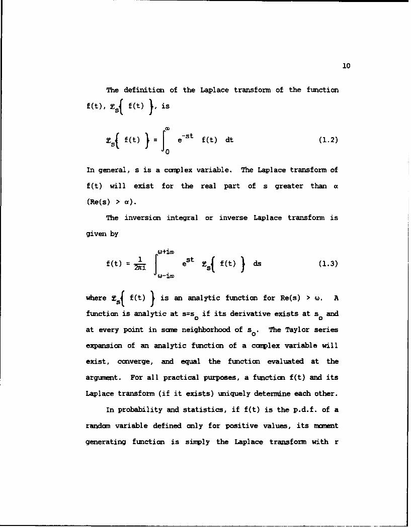
The definition of the Laplace transform of the function

f(t), zsf f(t)}, is

Z ~ } (t Jo e- f (t) dt (1.2)0

In general, s is a complex variable. The Laplace transform of

f(t) will exist for the real part of s greater than a

(Re(s) > a).

The inversion integral or inverse Laplace transform is

given by

f(t) J est Zs f(t) ds (1.3)

where -f ftM)} is an analytic function for Re(s) > w. A

function is analytic at s=s0 if its derivative exists at s and

at every point in some neighborhood of s o . The Taylor series

expansion of an analytic function of a ccrplex variable will

exist, converge, and equal the function evaluated at the

argument. For all practical purposes, a function f(t) and its

Laplace transform (if it exists) uniquely determine each other.

In probability and statistics, if f(t) is the p.d.f. of a

random variable defined only for positive values, its moment

generating function is sinply the Laplace transform with r

11

replacing -s in Eq (1.2).

1.3.2. FOURIER TRANSFM

The form of the exponential Fourier transform used in this

thesis is

,s{ f(t)} = e s t f(t) dt (1.4)

The Fourier transform is a function of the coniplex variable s.

If f(t) is a p.d.f., this definition corresponds to the

definition of the characteristic function in probability and

statistics. The characteristic function of a p.d.f. will

always exist but the nmnnt generating function of a p.d.f. nay

or ay not exist.

The inversion integral or inverse Fourier transform is

given by

where

f * () 1 im f(t) + 1im f(t) (1.6)tt 0 tlt 0

t<t t>to

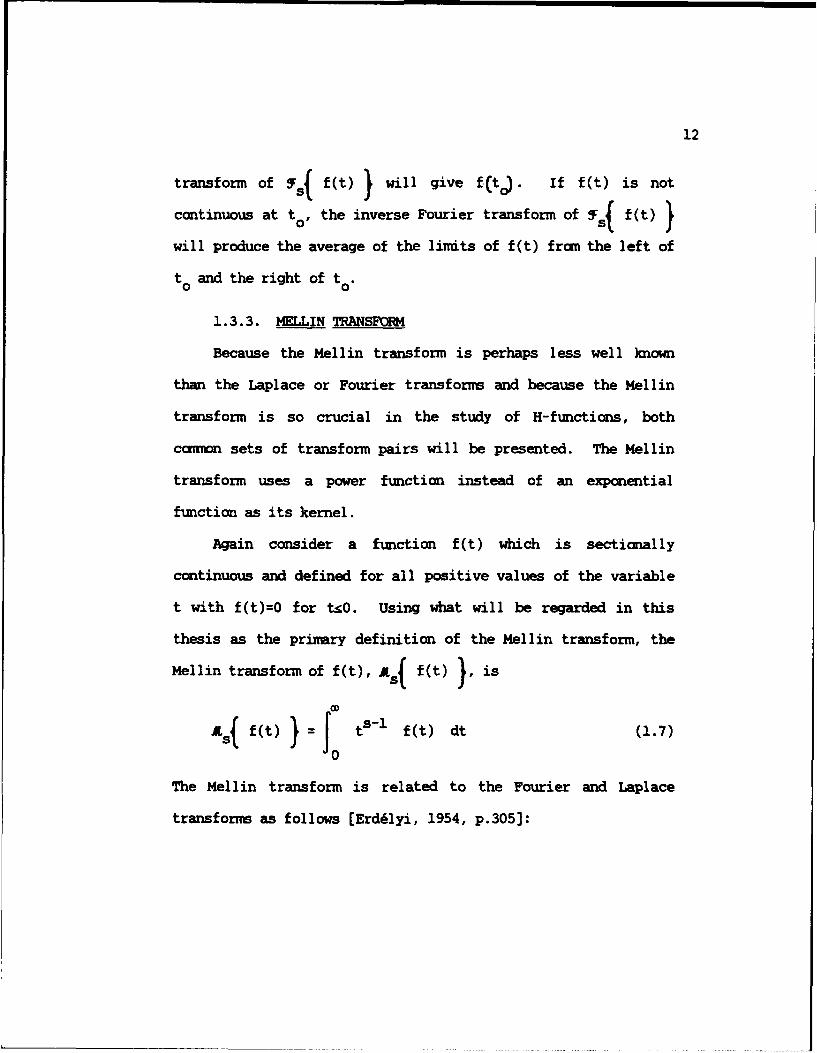
If f(t) exists and is continuous at t the inverse Fourier

12

transform of Y,( f(t) ) will give f(t). If f(t) is not

continuous at to, the inverse Fourier transform of Y f(t) }will produce the average of the limits of f(t) from the left of

to and the right of to.

1.3.3. MELLIN TRANPOIN

Because the Mellin transform is perhaps less well known

than the Laplace or Fourier transform and because the Mellin

transform is so crucial in the study of H-functions, both

com n sets of transform pairs will be presented. The Mellin

transform uses a power function instead of an exponential

function as its kernel.

Again consider a function f(t) which is sectionally

continuous and defined for all positive values of the variable

t with f(t)=O for t,o. Using what will be regarded in this

thesis as the primary definition of the Mellin transform, the

Mellin transform of f(t), A f(t) }, is

A(f(t) ) = Jo t S1 f(t) dt (1.7)0

The Mellin transform is related to the Fourier and Laplace

transforms as follows [Erd6lyi, 1954, p.305]:

13

f f (t) }= f-i{ f (et) (1.8)

-_ { f(et) }+ Z{ f(e-) } (1.9)

Again, s is a carplex variable. The Mellin transform

inversion integral, or inverse Mellin transform, is given as

1 ,(O+iCO

c1-i

As mentioned earlier, there is another important transform

pair also referred to as a Mellin transform pair. This

alternate definition will arise later when an alternate

definition of the H-function is given. The alternate

definition is

i~f(t) }=J t-rl f(t) dt (1.11)0

with inverse transform

f(t) = JVVC x r{J f(t) } dr (1.12)u-iCD

1.4. TRANSFU TICIS OF INDEHWIT RANDC4 VARIABLES

A canmn problem in statistical distribution theory is to

find the distribution of an algebraic combination of

14

independent random variables. The algebraic cumbination could

include sums, differences, products, and/or quotients of

independent random variables or their powers. It is important

to recognize that the algebraic combination is itself a random

variable and, therefore, has a probability distribution. The

task is to find this distribution.

Using the properties of mathematical expectation, it is

relatively easy to find the mean, variance, and other nxments

of the algebraic cumbination of independent random variables.

For example, the mean of the sum of two independent random

variables is simply the sum of the means of the random

variables. Finding the completely specified distribution of

the algebraic combination is usually much more difficult.

For simple ccubinaticns of independent randum variables,

the method of Jacobians is often employed. An appropriate

one-to-one transformation between the independent randum

variables in the algebraic cumbination and a set of new random

variables is first created. After finding the inverse

transformation functions, the Jacobian (the determinant of the

matrix of first partial derivatives of the inverse functions)

may be computed.

The joint p.d.f. of the newly defined random variables is

the absolute value of the Jacobian multiplied by the product of

15

the original densities with the inverse transformation

functions substituted for the variables. A great deal of care

must be used in determining the values of the new variables for

which the joint density is nonzero. Cnce this is done, the

desired marginal density can be obtained by integrating over

the complete ranges of the other new variables.

An example of the method of Jacobians will be presented

below. In most of the following sections, however, only the

result using integral transforms will be given.

1.4.1. DISTRIBUTION OF a SM

Let X1 and X be independent randn variables with

respective densities f i(x) and f 2(x), each nonzero only for

positive values of the variable. Suppose we want the density

of Y=X+X 2 . Using the method of Jacobians, we define W=X 2 so

the inverse transformations are XI=Y-W and X--W. The Jacobian

is

: n: (1.13)

1 0 1

The joint density of Y and W is

fywCY,w) = f1 (y-w) f 2 (w) 0 < W < y < C (1.14)

The marginal p.d.f. of Y can be obtained by integrating the

joint p.d.f. with respect to W over the range of W.

16

= J fl(Y-w) f2(w) dw (1.15)1~0

Eq (1.15) nay be recognized as the Fourier convolution

integral (Springer, 1979, p. 47]. This is no accident or

coincidence as the Fourier or Laplace transform could also have

been used to find the distribution of Y. It is well known that

the Laplace (or Fourier) transform of the p.d.f. of the sum of

two independent random variables defined for positive values is

the product of the Laplace (or Fourier) transforms of the

individual densities. Further, the product of two transform

functions, upon inversion, yields a convolution integral.

If the product of transform functions can be recognized as

the transform of some function, then the convolution inversion

is not necessary. The p.d.f. of Y is the function whose

transform is the product. When statisticians use the moment

generating function of each density to find the p.d.f. of Y,

this recognition approach is usually taken. one advantage of

using transform functions is that the procedure easily extends

when the distribution of the sum of three or more independent

random variables is desired.

Finding the distribution of the sum of independent random

variables with certain special distributional forms is

considerably sinplified. Several of these cases are covered in

17

the following subsections.

1.4.1.1. INFINITE DIVISIBILITY

Although a ccmplete discussion of infinite divisibility is

beyond the scope of this thesis, its definition is given below

[Petrov, 1975, p. 25).

A distribution function F(x) and the correspondingcharacteristic function f(t) are said to beinfinitely divisible if for every positive integer nthere exists a characteristic function fn(t) such

that

f(t) = (fn(t))n

In other words, the distribution F is infinitelydivisible if for every positive integer n there

exists a distribution function Fn such that F=F*n .

Here F*n is the n-fold convolution of the functionn

F.nCcmnon exanples of infinitely divisible distributions include

the normal and Poisson distributions.

1.4.1.2. SPECIAL CASES

The distribution of the sum of independent randan

variables with certain distributional form is well known and

imrediately available. For exanple, the sum of n independent

and identically distributed randmn variables with a Bernoulli

distribution with parameter p has a Binanial distribution with

parameters n and p. Similarly, the sum of independent

geometrically distributed random variables with a caot

18

parameter has a negative BinaTial (or Pascal) distribution.

In continuous random variables, the sum of n independent

and identically distributed random variables with an

exponential distribution with parameter I has a gamm

distribution with parameters n and X.

1.4.1.3. REPRODUCTIVE DISTRIBUTICNS

A probability distribution is "reproductive" if it

replicates under positive addition of independent random

variables with the same distributional form. The normal

distribution is reproductive since given that

X.,- Normral (Pit a2) X- Normral P( 2

X1 and X2 are statistically independent, and

YX1+X2

then

Y ~ Normal ( P Pi+ 2 o+02

Other examples of reproductive distributions include the Chi-

Square and Poisson distributions.

It is well known that the gam distribution is

reproductive provided the scale parameter, X, is the same for

each random variable in the sum. In particular, if

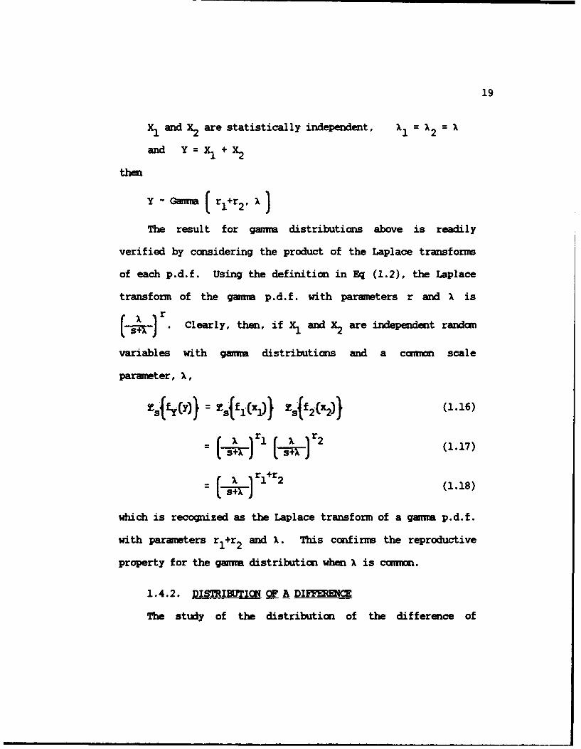
19

X1 and X are statistically independent, x= 1 2

and Y=X1 +X 2

then

Y - Gamma ( rl+r2 , X]

The result for gamsa distributions above is readily

verified by considering the product of the Laplace transforms

of each p.d.f. Using the definition in Eq (1.2), the Laplace

transform of the gamma p.d.f. with parameters r and X is

rrdo(s1 3 rd Clearly, then, if Xand X2are independent random

variables with gamma distributions and a caiomn scale

parameter, X,

T-s{fY(Y)} Z5 ff1 (xl)} Z5 {-f2 (x2 )} (1.16)

S r)~l ( 1 r2 (1.17)

, r 1r+r 2 (1.18)

which is recognized as the Laplace transform of a gamma p.d.f.

with parameters r1 +r2 and X. This confirms the reproductive

property for the gamma distribution when X is comn.

1.4.2. DISTRIB7MION OF A DIFFERENCE

The study of the distribution of the difference of

20

independent random variables has received nuch less attention

than for the sum. The norml distribution is one notable

exception since given that

X1 and X2 are statistically independent, and

y x 1 -X 2

thenY Normal2 2

Norm l i-P2, oi+cr2

If X1 and X are independent randan variables with

respective densities f 1 (xl) and f 2 (x 2), each nonzero only for

positive values of the variable, then the density of Y=X-X 2 is

the inverse Fourier transform [Springer, 1979, p. 59]

for -w y < < (1.19)

1.4.3. DISTRIBUTIC OF A PROWCr

If X1 and X2 are independent randan variables with

respective densities f,(x) and f 2 (x 2), each nonzero only for

positive values of the variable, then the density of Y=(Xl) CX)

is the inverse Mellin transform [Springer, 1979, p. 97]

21

f =y 3 Y-S At. fl(z) f Js 2 x2) } ds

for 0 < y < w (1.20)

1.4.4. DISTRIBUTIC4 OF A QTIENT

If X1 and X2 are independent random variables with

respective densities f Cx1 ) and f 2 (x2), each nonzero only for

Positive values of the variable, then the density of Y is

the inverse Mellin transform [Springer, 1979, p. 100]

i Y,- '& s--{ fI (xl) ) ,_o{ f2(x) f ds

for 0 < y < m (1.21)

One caoicn examPle of the quotient of two independent

randm variables lies in the derivation of the Snedecor F

distribution [Springer, 1979, pp. 328-9]. If

X1 - Chi-Square (P) X2 - Chi-Square (w)

X, and X2 are statistically independent, and

xl

y _ V

then

Y - F (u, )

22

1.4.5. DISTRIBUTION OF A VARIATE TO A POWER

If X is a continuous random variable with density f(x),

nonzero only for positive values of the variable, then the

density of Y= P is the inverse Mellin transform [Springer,

1979, p. 212](s+i

for 0 < y < a (1.22)

One common example of a variate to a power is finding the

distribution of the square of a standard normal (zero mean,

unit variance) randm variable. If X - Normal (0,1) and Y=X

then Y - Chi-Square (1). The same result holds if X has a

half-normal distribution with o 2 =1 [Springer, 1979, pp. 213-4].

1.4.6. MbD4NTS OF A DISTRIBUTIOM

If X is a continuous randn variable with density f(x),

nonzero only for positive values of the variable, then the

mraients about the origin of f(x) are

= f OD xr f(x) dx (1.23)0

provided the integral in Eq (1.23) exists.

23

There is a natural relationship between the integral given

in Eq (1.23) and the Mellin transform of the function f(x)

given in Eq (1.7) or Eq (1.11). Using the Mellin transform in

Eq (1.7) we can write

Mr = dr+l[f(x)J (1.24)

This relationship simplifies the computation of maments for H-

functions and H-fmction distributions.

CHATM 2

THE H-FUNCTICI

The H-function is a very general function, encompassing as

special cases nearly every named mathematical function and

continuous statistical distribution defined over positive

values. Although the H-function does not enjoy an extensive

popularity and acceptance in the fields of mathematics,

probability, and statistics, this is primarily because

mathematicians and statisticians have not yet learned of its

versatility and power. Most analysts are not familiar with the

H-function, and many who have seen the H-function definition

way have been disquieted by its overt complexity. This is

unfortunate because practical use of the H-function does not

require extensive knowledge of complex analysis and integral

transform theory.

Mathematical functions defined by an integral which do not

have a closed form representation are commn. Examples include

the gaima function, the error function, and the cumulative

normal probability density function. In all of these cases,

the function is usually evaluated with the help of tables. The

24

25

H-function is another example of such functions. Like all of

the transcendental functions (e.g. e , sin x, cos x), it must

be evaluated using an infinite series expansion. A FRTRAN

computer program is available [Cook, 1981; Cook and Barnes,

1981) which will evaluate the H-function at desired values once

the parameters are specified.

Fox [1961] first developed the H-function as a direct

generalization of Meijer's G-function. Mathai and Saxena

[1978] presented nany useful properties of the H-function and

listed the nmthematical functions that are known to be special

cases of the H-function. More recently, Prudnikov et al [1990]

compiled entensive results of all special functions, including

H-functions.

2.1. PRIMARY DEFINITION

The prinary definition of the H-function as used in this

thesis is:

H(cz) lp n[czJ = 1 p4 cz : f(A') ; rrbB viiP, q =p q ff ij

i=1,....,p j=l,.., q

1 jn + +B~) n r(1-a-As)1j= i=l (cz) - s dsn ra+As r[l-b .-B is)iC i=n+l • aj--Im+1%

26

where z, c, and all a. and b. are real or ccrplex numbers, all

A. and B. are positive real numbers, and m, n, p, and q are

integers such that Orz'q and 0snap. Empty products are defined

to be unity (1). The path of integration, C, is a contour in

the complex s-plane from w-im to w+iw such that all Left Half-

Plane (LMP) poles of 11_r(b +Bjs) lie to the left of C and all

n

Right Half-Plane (RHP) poles of I] rli-a.-A s) lie to the

right.

Although the H-function is defined for the complex

variable z, we will often restrict our attention to the real

variable x. Further, since the H-function is not valid for

non-positive real values of z, we will often consider only

positive values of the real variable x.

The definition of the H-function in Eq (2.1) nay be

recognized as the inverse Mellin transform where the transform

pair is as given by Eq (1.7) and Eq (1.10).

H-functions are somtimes classified according to their

order, the number of gamma terns in the integrand (p+q), and

the placement of those terms. References will be made to

certain classes of H-functions as n n with particular valuespq

for the parwieters m, ni, p, arid q.

27

2.2. ALTENATE DEFINITIC

It should be noted that there is an alternate, but

equivalent definition of the H-function:

H(cz) = Hmn~ cz : {(aiAi)} ; {(bjBj)}

i=1,. P ,p j=1',...,-qn Ib- n laiAr-1 (cz) r dr

n I (a -A r)j r~l-b .+B .r)iC i=n+l --mrl # J

(2.2)

where the restrictions on the variable and parameters are as

above. Here, the path of integration, C', is a contour in the

complex r-plane from P-im to P+im such that all RHP poles of

mr=1 b-Br) lie to the right of C' and all LHP poles of

nr(l-a.+A.r) lie to the left.

Eq (2.2) above can be derived fran Eq (2.1) by the

substitution r-s. Under this transformation, L=-( since the

substitution r=-s rotates about the imaginary axis all poles of

the integrand and the contour, C, into a contour, C', which

also separates the new UIP poles from the new 1IP poles in the

standard munner and direction. Again, the definition in

28

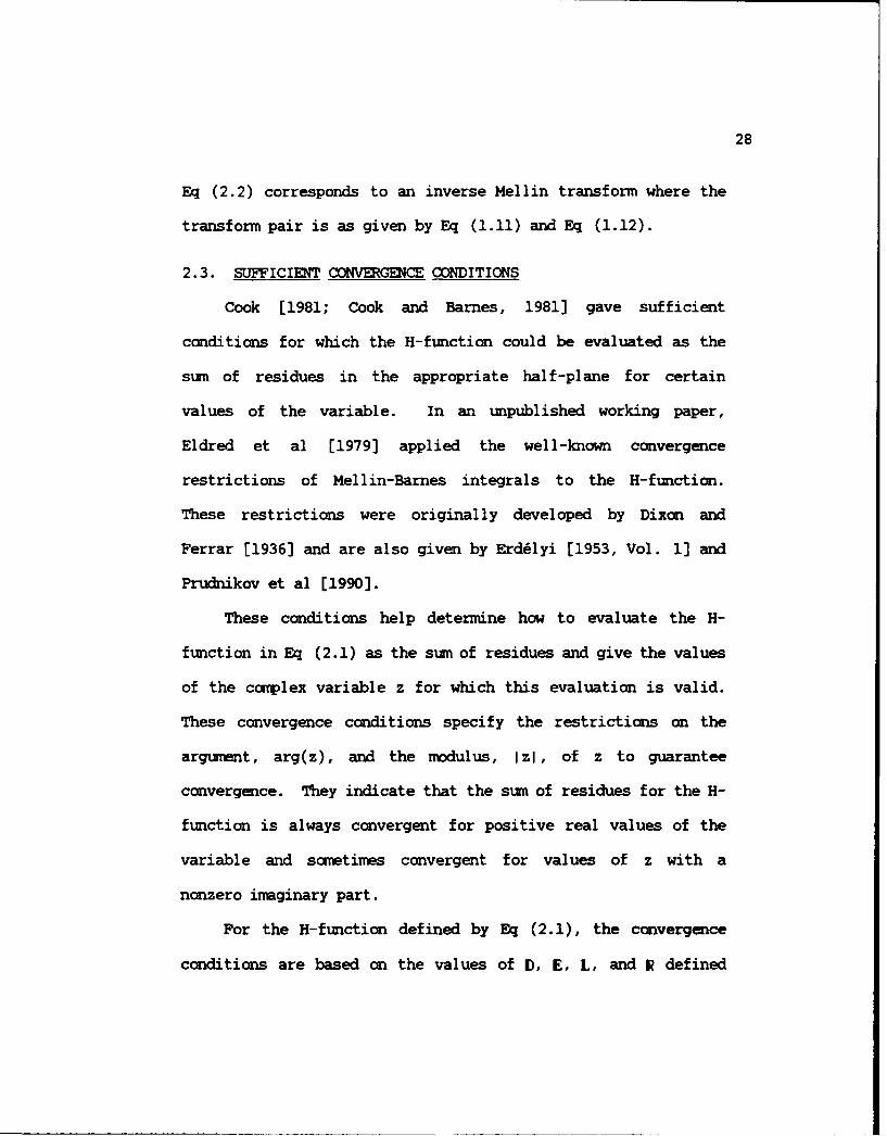
Eq (2.2) corresponds to an inverse Mellin transform where the

transform pair is as given by Eq (1.11) and Eq (1.12).

2.3. SUFFICIENT CONVEGENCE CONDITIONS

Cook [1981; Cook and Barnes, 1981] gave sufficient

conditions for which the H-function could be evaluated as the

sum of residues in the appropriate half-plane for certain

values of the variable. In an unpublished working paper,

Eldred et al [1979] applied the well-known convergence

restrictions of Mellin-Barnes integrals to the H-function.

These restrictions were originally developed by Dixon and

Ferrar [1936] and are also given by Erd~lyi [1953, Vol. 1] and

Prudnikov et al [1990].

These conditions help determine how to evaluate the H-

function in Eq (2.1) as the sum of residues and give the values

of the complex variable z for which this evaluation is valid.

These convergence conditions specify the restrictions on the

argument, arg(z), and the modulus, I zI, of z to guarantee

convergence. They indicate that the sum of residues for the H-

function is always convergent for positive real values of the

variable and sometimes convergent for values of z with a

nonzero imaginary part.

For the H-function defined by Eq (2.1), the convergence

conditions are based on the values of ID, E, L, and IR defined

29

as:

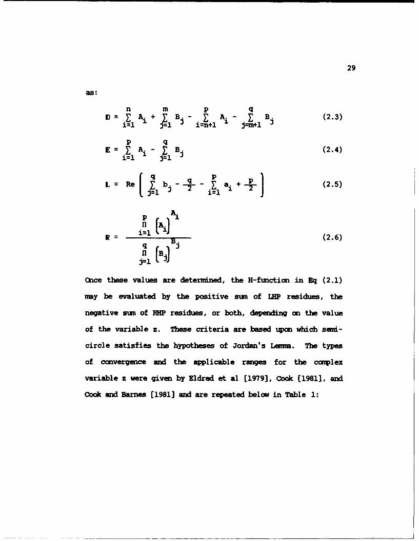
n m p qID= EA =+ Bj E Ai E B. (2.3)

i=1 3=1 i-n+l j-n*1 l

p qE=EA Bj (2.4)

_ q pL : eb -- - a. + -- (2.5)

=1

i= (A3) (2.6)

q (Bjj=l j

(nce these values are determined, the H-function in Eq (2.1)

nay be evaluated by the positive sum of LHP residues, the

negative sum of RHP residues, or both, depending on the value

of the variable z. These criteria are based ton which send-

circle satisfies the hypotheses of Jordan's Lema. The types

of convergence and the applicable ranges for the caplex

variable z were given by Eldred et al [1979], Cook (1981], and

Cook and Barnes [1981] and are repeated below in Table 1:

30

Table 1. Convergence Wm for H-Functins of E (2.1)

TYPE D) E L H(cz) Izi Iarg(z)I

I >0 <0 )IX + LHP res >0 <x <-AD

II ko <0 AM +E LHP res >0 < n I-RV

III >0 >0 >) -E RHP res >0 <- , <--D

IV k0 >0 ' -4RP res >0 < n , x--

ELHP res < 1

V >0 =0 10 d< , <--v

-m res >

CIRLRU res < 1

VI 20 =0 <0 O < x I ---£ m res > 1_

cS

where, if L < -1 in Type VI convergence, one may use the sum of

either LHP or RHP residues at I zg I = 1 Type VI convergent

H-functions play a central role in several new results given in

Sections 2.5, 2.6, 3.6, and 4.3.

Because there was same disagreement [Springer, 1987] about

the validity of the convergence conditions given by Cook [1981;

Cook and Barnes, 1981], it was necessary to develop the

corresponding convergence conditions for the H-fumction in

31

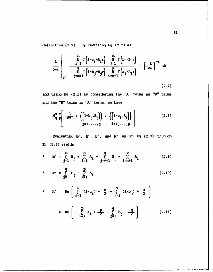
definition (2.2). By rewriting Eq (2.2) as

n m

1 nr(.1-ai+A~r * n r(kj-Bjr) -

i=1 r) J dr2ni q

I' n-m~ r (1- i B ) i=npl r i - i r)

(2.7)

and using Eq (2.1) by considering the "A" term as "B" terms

and the "B" terns as "A" terms, we have

On 1n :L {(1-bjBj)} ; {(1-aiAj)} (2.8)q ~l p • ciz .. ,

Evaluating ID', E', L', and R' as in Eq (2.3) through

Eq (2.6) yields

In n q pI 1 = j BjE iA + A1 (2.9)3=1 i'= j-v i=n

q p• E' = B.- Ai (2.10)

S Re (-a (1-bj)

Re-r + b - (2.11)

32

IR = (B))' (2.12)p A.

i =1 (Ai) 2

Ccuiparing Eq (2.9) through Eq (2.12) to Eq (2.3) through

Eq (2.6),

D' in Eq (2.9) 1) in Eq (2.3) (2.13)

E' in Eq (2.10) =(-1) [ E in Eq (2.4) J(2.14)L' in Eq (2.11) = L in Eq (2.5) (2.15)

R' in Eq (2.12) = [ IR in Eqi (2.6) (2.16)

These rel ation~ships all ow the corresponiding convergence

types for H-fumctions def ined by Eq (2.2) to be written.

Table 2 lists these types of convergence.

33

* Table 2. Convercence Types for H-Functions of _1 (2.2)

TYPE D$ E' L' H(cz) Izi I arg(z) I

I >0 <0 >E1' -IM res >0 < X < -t-

II 0 <0 v'a -MP res >0 < X Iwo

III >0 >0 )E'LJ +E LHP res >0 < X < 7-'

IV kO >0 a',' +E LHP res >0 < X -

-M res <A-V >0 =0 k0 < X , <-i--

+E LHP res > R'

-1IP res < IRc

VI 10 =0 <0 <E L, r->-<LHP. res > R

where, if L' < -1 in Type VI convergence, mne nay use the sum

of either IMP or RHP residues at I zI = R'c

As expected, there is a ccmplete interchange of LHP and

RHP poles. Type I convergence for the H-function of Eq (2.2)

in Table 2 corresponds to Type III convergence for the H-

function of Eq (2.1) in Table 1. Similar statements apply

between Types II and IV, III and I, and IV and II. Even Types

34

V and VI in Table 2 correspond to Types V and VI in Table 1

when considering the relationship between R and R' in

Eq (2.16).

Either set of conditions is sufficient, but not necessary

for the appropriate H-function to converge. Still, nearly all

of the mny special cases of the H-function satisfy the

convergence conditions. Further, the conditions consistently

and correctly identify the valid range of the variable over

which the H-function representation equals the special case.

Cne should not think of these conditions as constraints on

the H-function, as Springer [1987] did. Instead, they should

be viewed as a sufficient tool to determine how the H-function

can be evaluated with the sum of residues - those in the IMP or

those in the RHP. Depending on where Jordan's Lewma is

satisfied, residues at the IMP poles, or RHP poles, or either

are summed for different values of the variable. These choices

are succinctly given in Table 1 (and Table 2) for most cases of

interest.

To demKtrate that the convergence conditions are

sufficient, but not necessary, consider the following

representation of e for x>O as a Meijer G-function [Prudnikov

et al, 1990, p. 633]

35

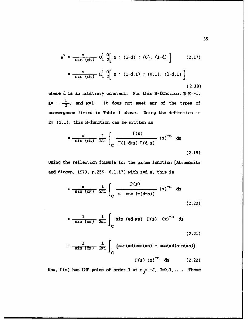
e = s[() G1 x (1-d) ; (0), (1-d) (2.17)

sin___ (5i) 1

2[ 1 2I 1sn H . x :(1-d,1) ; (0,1), (1-d,1)

(2.18)

where d is an arbitrary constant. For this H-function, )=E=-I,1

L= - and R=1. It does not meet any of the types of

convergence listed in Table 1 above. Using the definition in

Eq (2.1), this H-function can be written as______ 1 r(s) ( -s

sn 1cbz)) W(x) dssin (d) -i 1C F(l-d+s) r(d-s)

(2.19)

Using the reflection formula for the gamn function [Abramowitz

and Stegun, 1970, p.256, 6.1.17] with z=d-s, this is

R 1 [r(s)W Sdsin (arc) 'Y 1 c (x) -s ds

(2.20)

1 ~ J sin (nd-ns) r(s) (x)-s dssin (WTW 1

(2.21)

1 ] (sin(nd)cos(ns) - cos(nd)sin(ns))

r(s) (x)-s ds (2.22)

Now, r(s) has LHP poles of order 1 at s= -J, J=0,1,.... These

36

are the only poles of the integrand. At these values of s,

sin(ns) vanishes and cos(us) = (-1) Using the residue

theorem to evaluate the contour integral as the sum of residues

produces

s1 s)~ 2n [(-1)Jsin~nd)] [(-1)~ xsin (dn) J

(2.23)

-e Q.E.D. (2.24)

This proves that the convergence conditions given in Table 1

are sufficient, but not necessary, for the H-fuction to

converge.

2.4. PROPERTIES

Amnag the useful properties of the H-function are the

identities dealing with the reciprocal of an argument, an

argument to a power, and the mutiplication of an H-function by

the argument to a power [Carter and Springer, 1977].

37

2.4.1. RECIPROCRL OF AN ARGMT

Hm[ 1 f-b.BVI ; (hl-a. .Afl 1 (2.25)q P1 z I i

2.4.2. ARG3~IT TO A PCWER

1 4 z : {(:A'h)} ; {(b, B2)}] (2.26)

for c > 0

38

2.4.3. I4LTIPLICRTICt BY THE ARGUMET TO A FIWR

z c 1P z : iA) (jB)p ~,., j=,.,

=,p n[ z {(ai+A. cAj)} ; b+ c, 1 (2.27)i=l,..., p j=l,...,q

2.4.4. FIRST REDUCTICN PROPmTY

If a pair of "A" terms and a pair of "B" terns in an H-

fmction are identical and one is in the numerator of the

integrand and the other is in the denainator, then it is

equivalent to an H-functin of lower order. Specifically,

[Mathai and Saxena, 1978, p. 4]

i[ z : flai,Ai)} ; (ubj,Bj))}, Jalpn-a q- . A,%_ Hpm 1 z : f~iA1); fj,Bj) (2.28)

" =2....,p j=l,..., -q-1

provided n>O and q>m. Also,

39

II1i , q,p-1 ,...,(bB) ; =1.A.

,,! -n1) fr(b.,Bj))

=Hm I - z : (a 1,A1) (2.29)i , ,p-i j=2,...,q

provided m>0 and p>n.

2.4.5. SECOND REDUcTICH PROPET

Bodenschatz and Boedigheirrer [1983, pp. 11-12] discovered

another way in which the H-fumction can reduce to one of lower

order, at least in the limit. If any Ai or B. is close to

zero, that gam term in the integrand of Eq (2.1) is

essentially a constant. Thus,

nz : [i rr1p q p q-1iIiJ (I"=1....,p j=2,...,q

(2.30)

for B1 m 0 and m>0. Here, the synbol o means the limit of

H- n[z] as B1 -.0 is given by the right side of Fq (2.30).p qz]aB7

40

,hCin[Z]s ft' n z aiA)pq r(.-bq) Ip q-i1

{ (il s3)) I (2.31)

for B. w0 andmnq.

p q~z f r(J-a]) H..J 1 q {(aiAi)}

{(bif} I (2.32)

for A, ow 0 and n>0.

q r.(ap-i j=i....,q J(2.33)

for A. 0 and n~p.

* 2.4.6. HIRACIA RELRTIQM~IPS OR-M

On significant, but surprisingly simple, discovery was

that whole classes of H-functions are udbedded in other

41

classes. For example, the 0 0 class of H-functions is a

proper subset of both the H1' 0 and 4 0 classes of H-functions.1 1 2~

These classes, in turn, are erbedded in other, higher orders of

H-function classes.

This newly discovered hierarchical relationship among

classes of H-functions results in several new ways in which

certain H-functions can reduce to H-fumctions of lower order.

Further, while the first and second reduction properties listed

above are readily apparent and easily understood, the new

reduction properties are less transparent.

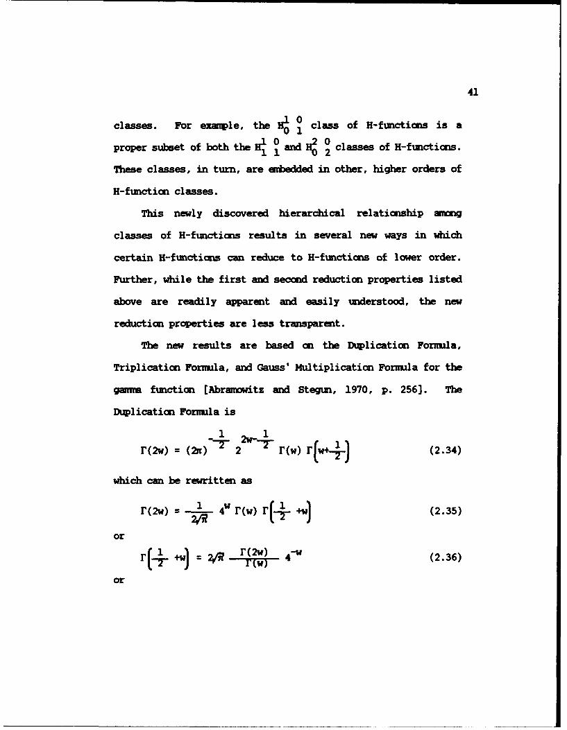
The new results are based on the Duplication Formula,

Triplication Formula, and Gauss' Multiplication Formula for the

gamma function [Abramowitz and Stegun, 1970, p. 256]. The

Duplication Formula is

-1 2w 1

r(2w) =(2n) -72 r (w) r (W++2- (2.34)

which can be rewritten as

r(2w) 1 4w r(w)r(+ +w (2.35)or(2w)

orr[-+ +w): =;R r(2w) 4 W(2.36)

or

42

r(w) = 2R r(2w) 4 (2.37)r(+ +w)

Any gmms function present in the integrand of Eq (2.1) in

the definition of the H-function can be replaced with an

equivalent expression as in Eq (2.35), Eq (2.36), or Eq (2.37).

Terms of the above equations which do not involve gmmma

functions can be carbined with the paramters k or c in the

definition of the H-function. Using Eq (2.35), a 0 H-

function nay be rewritten as a 0 H-function. Using

Eq (2.36) or Eq (2.37), a 0 H-function way be written as a

H0 -function. The H-functions resulting fra Eq (2.36) and

Eq (2.37) appear distinct, but can be shown to be equivalent.

I will state these new upgrade and reduction results for

first order H-functions as theorem and provide proofs. The

proofs sinply use the argument to a power property in Eq (2.26)

to change B to unity, the definition of the H-function in

Eq (2.1), and one of the fors of the duplication property in

Eq (2.35) to Eq (2.37).

STheor2.1. H 0[ cz : ,Bb) -

H1. 4B cz: (b-h.4..B) ; (2b-1,2B) ](2.38)

43

Proof:

1, rr

,TH r c 45- 4 -s (cz) ds

using Eq (2.36) with w = 1-+

1 r 2b-1+29 ( siVT..34~ ~ B~ dJsb~.s~

1i 0i ( 4 B).W (b-+,]1) ;(2b-1,2)

- I -Hi 04Bz * (.7+,) (2-1,2) (2.39)

Q.E.D.

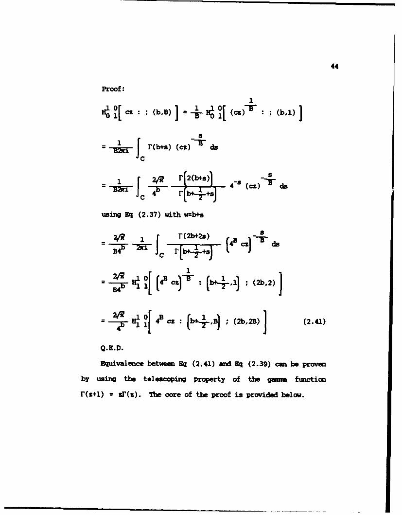
* Theorem 2.2. i0[ cz ;(bB)]

44

Proof:1

J (b+s) (~cz) 05

C

29 r r2(b+s)1

4-C ( cz) ds,

using Eq (2.37) with wrb+s

29 1 _ _ _+s)-

S-[ (.,2al :L++o (b,2+ .(.1

Q.E.D.

Equivalence between Eq (2.41) and Eq (2.39) can be proven

by using the telescoping property of the gumm functim

r(z+i) = zr(). The core of the proof is provided below.

45

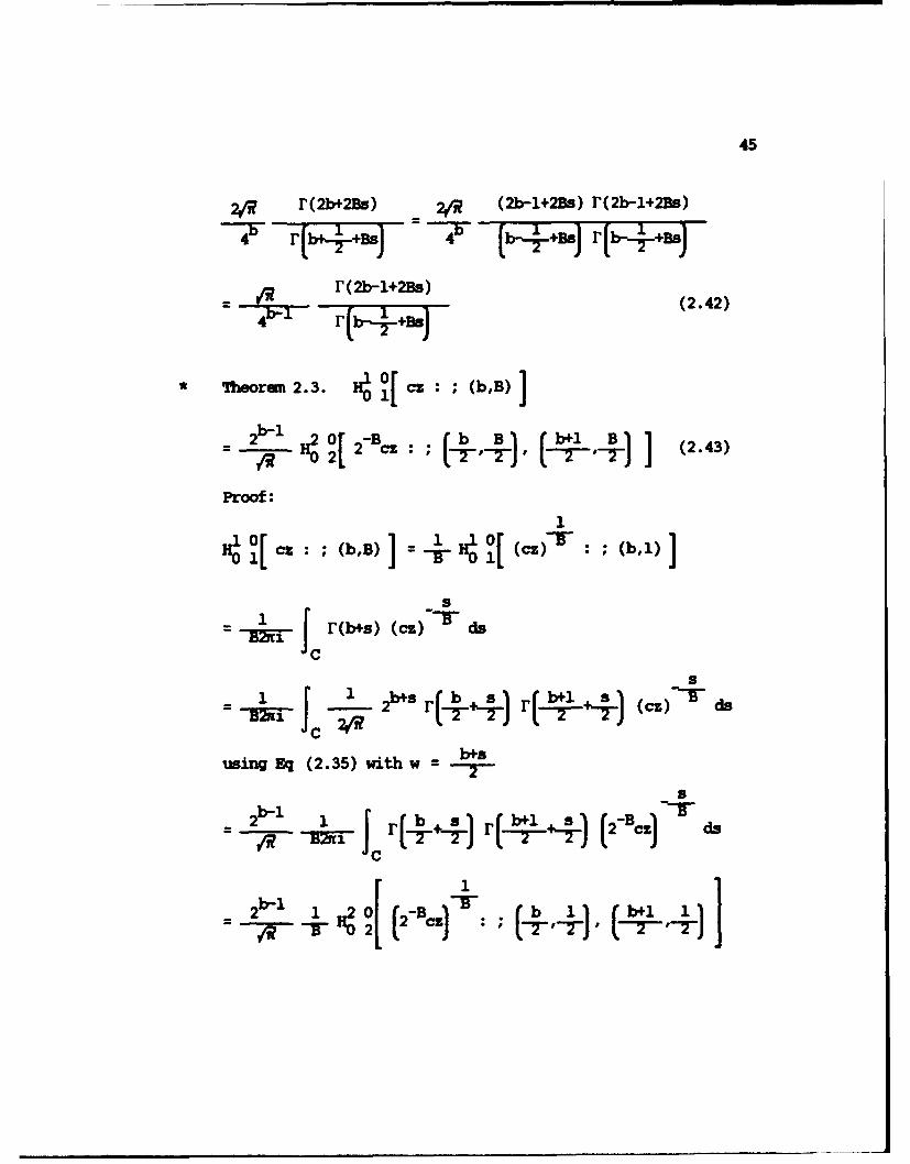
2w r(2b*2Bs) 2v'R (2b-1+2Bs) r(2b-1.2Bs)

4-r~h+s -4 [b+sJ r [i4+Bs)

R 'I-r(b12s (2 .42)

* Thorem 2.3. H4 IC 0 : ; (bB)]I

Proof:

~ r(b+s) (cz) cia

ccs

using Eq (2.35) with w = ..s

2 b-1 1 Jr + r(J . ) (2-Bc d

- 1~' '0 (2 Bcz): ;( )(b+11)

46

2b-1 [ 2BcZ (2.44)

Q.E.D.

Upgrade and reduction results for the more general class

of H-functions ep n can be proven using the sam steps as inp q

the above proofs by working on any gwmu function present in

the integrand of Eq (2.1). Since the proofs are very similar

to those already provided, Theorem 2.4 through 2.7 will be

stated without proof. The generalized results are

* Theorem 2.4. p .4 cz : f fa.,Aifl ; 'b.,Bj))

"=i,...,p j=,...,q J

(2b1 , 1), {(bj,Bj) 1 (2.45)

j=2,. ... ,qJ

47

2b1-1 n 2-Bz: aA)

I i=1, .... .

b 1 B Bl ' 1-2- mI , l(bjB~jJJ (2.46)

for m>O.

* Theorem 2.5. Ir 4 cz : ffj).); f(bjBjli]a~ -q

4= p nf 4 - pcz : {(aiA1 )} , 2p2.

P q+11

L~~ . p-1

=~ ...

1 , 4 2cz :{(aiAi)} ,~

2~- '--- tb,BEjJJ (2.48)j=1,... ,qj

for p>n.

48

* Theorem 2.6. HP 4 cz (~B}

2fl 4q+l (2,1,A) { taiFjkiJ

4 i=2. ... 'p

{(b jBj)}I (a I-,A, (2.49)

1 ~ A a 1 A,), (aj+1A,)Ho3 2 cz '

{ (aiAi)} ; {(bjBj)} (2.50

i=,.. p =1.A

for n>O.

49

Theorem 2.7. g cz : (( 11 i) ( lijjJi=1,...,p j=l,...,q I

41- H B

qV p+I q q i -Y q)'

i=l,... ,p

{(bi#Bj)} , (2b4-1,2%q) I (2.51)j=l,... ,q-1

b q--2 i=,... ,p j=l, • .. ,q-1

, - - - I(2.52)for qxn.

Similar results are available by using the triplication

formula or Gauss' nultiplication formula. For example, using

the triplication formula, it is possible to show the 0 c

of H-functions is also a proper subset of both the 0 and

10classes of H-functions.

* 2.4.7. GRMf IZlNG CMSrT

Bodenschatz and Boedigheimer [1983; Bodenschatz et al,

50

1990] gave the first H-functiom representations which

recognized the existence of a positive generalizing constant,

u. They showed that for certain natheutical functior and

statistical distributions, the Aiand B. parueters need not

equal unity. They gave some new generalized H-function

representations, but did not state general conditions under

which a generalizing constant was possible. These general

conditions will be given below as four theorems.

* Theorem 2.8. If m>O, pn, A=B1 , and ap-b 1 =1, then

p qj c f(a.,AiI , fbl+1,Bl ; rb,Bl) f (bjB)i=l,...,p-1 j=2,....,A

j=2,... ,q

for u>O.

Proof:

p q=,..

[ 1,.....p-1

51

r m iij)

= 1 j=2 (bi 1- 1 As rb+~2i p-i q s bllBs2nn nr(a+Ais) jnr (1-bj-B~) rb++~

c i---s

(cz)'ds

nI rjb+Bjs) it' rI1-a1-AisI

-n j21 qJj i1

(cz) -s ds

m2 j~~Bs) 1 ~~iA

(cz) -s ds

m (bj+Bjs) nr u 1 u~j=2 l(

27(2. n r~a+Ais) n ri-b-Bs r +1Bs

(cz) -s d

52

=Um 4p cz : ffaj:Ai)) (ub1+iUB11

(UbiiUBi), i j#B) (2.54)

Q.E.D.

Theorem 2.9. If m)>O, p~n, BAand b -a =1 then

n~~ cz : (a&,A3.)} , (a,A) ; (a,+iiA), {(bjBj)}

[ i1l,. .. ,P-1 j=21 .... A

C c : I(iA) upt.

(ul~~p {(bjBj)} (2.55)

j=2,. .. ,J

for u>O.

Proof:

n'1 cz : ljaiAi)} (a,,A) ; (a,+1iA,)1 ,{(bjBj)}

p q1..,- 2...,

53

1 j r(b+e) in r (1-ai-A.,s) rfa,+1+A,5s

pnr (a1+As) n r (-bj-Bjs) ra+~

c i--n~ i---s

(cz)'ds

I ii r (a.+A.s n~ r (1-ai-A. S) (pi

i=2 +1 31 i l -s

(cz)sds

nr b .Bjs) nI r(i-ai-Als)

u2fi P-1 (ai+Ais) jr q 1b-~) (aus

(cz) -s d

54

n r~bi+B1 r(1-ai-Ais)

j=2 rb+s) iIl

I I r (a.+AisI jI r'i 1-bj-BjsJ

r ua,+uhpsl (ci) -s ds

r ua +u Se

(ua,+iiu&i.)i {(i, )j} 1) (2.56)

j=2,... JqQ.E.D.

55

*Theoran 2. 10. If n>0, q~m, A,=Eq, and a 1 54q=1, theni

,pncz qj (bq+1,Bq), fjaA4} ; (jB) (4,)

p uH 1 cz : rub,+l,ul T.,.f

{( (llai)} ) uq~~~ (2.57)

for u>O.

Proof:

Ip[ cz (bq+1,B~J, {(a,,A,)} ;(jB) (b,B

i=2,...,p j1l,.. .,q-,

m Bj n1n r(b+s) iZ r(l-a1-Ai s) r R-bq4B

27(1 np rflAs)qr(-b-B jsJ r 1-b.-Bqs

(cz) -s cia

56J m1 n r(b i+Bjs) n2 r(-aA)1

n r (a1 +A -s) 'n r (-bj-Bjs) -bq-Bqs

(cz)- ds

u n r b+B nrILa-Ais-j=1 (liis =

nf ~ r(ai+A I [ni r(-bj-Bjs) UbqUuBqs

(cz) -s ds

u n~ r n+Bs r (l-a 1 -Ais) r 'xD-Bs)

2rd3 ,p q-1 r FJ nrai+A,.sJ n (1-b ,-B is) 6l1ubq Uqs)

(cz) -s d

57

P 1cz : rub+l11B.), ffa. Kill

{(bj:Bj)) , (ubqiu!Bq (2.58)

Q.E.D.

* Theorem 2.11. If n>O, q)m, Bek,3 and b-ai~,te

pq 1

u q cx (uaiiuhA)i {(ai,)}

i=2, ... Alp

{ (bklli)} , (ua1 +1I~uA,) 1(2.59)j=1, . q-1

for WQO.

Proof:

c~lcz (aiiA,4. {(a±,Al)} ; {(b,,Bj)} (ai+IA)1

[ ~~i=2,...,pj1..,-J

58

'n ribj+Bjst nFr~-I-r1-a.-AAsj~l i=2 Sij 1a-

2xi p -. r -a-Alsi n ~+r~ai+AisJ jn r-bj-BjJ1-

i--n~l is

(cz) ds

- 1 J r(bj+BjsJ in rlii-A) (a-

(cz) 'ds

J j i i~yns) - 1 21 (1bB ) (-uaru S)

u~i nr (ai+Ais) q -i -sjs

59J m n1 j _ (bB i=2 (

u2mi pAi q-1

n 1'ai n r l-Ul-Bjs)

r 1-ua_-uasl (c) - s ds

4 c. cz : rual,uAiI. ffa.,A.1li=2,... Op

{~ (j,B)} , (ual~luR) 1(2.60)j=1,... ,q-1

Q.E.D.

2.4.8. IRIVATIVE

It is well Iknown that the derivative of an H-function is

an H-fumcticn of higher order. Let the rt h derivative of

lp~ n(zj be denoted by H(r)[z]. If all real b. are such thatp qJ

- < I for j=l,...,m then the rth derivative of n n[z] is

[Mathai and Saxeam, 1978, p. 7; Cook, 1981, p. 83]

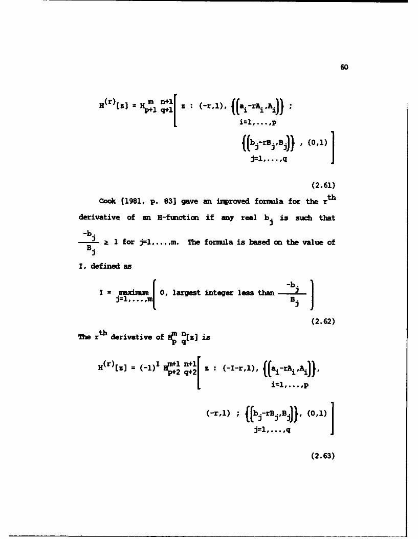
60

H(r)[z] = H Pmn+i z : (-r,1), .a.-rA.,J.i

[i=1,... op{( (ji-r~j,Bj),) (0,1)1

j=1,. . . ,q

(2.61)

Cook (1981, p. 83] gave an inproved formula for the rth

derivative of an H-function if any real b is such that

-b.-3 2 1 for j=l,...,m. The fornula is based an the value of

B.

1, defined as

I = nxi. 0, largest integer less than BJ

(2.62)

The rth derivative of IC '1z] is

H (r)(z] = (-1) 1 l nI2 z : (-I-r,1), (ai-rAi,,A)),

i=1,...

(-r,1) ; (jb j-rBj1 ,Bj)}. (0,1)1

j=1,... ,q

(2.63)

61

2.4.9. LU31ACE TRANSFORM

It is well knmow that the Laplace transform of an H-

function is an H-functimn of higher order. If all real b. are

-b-such that < 1 for j=l,... ,m then the Laplace transform ofB3

,in npczJ is [Springer, 1979, p. 200; Cook, 1981, p. 35]p q

T-fH(cz) I J f e r H(cz) dz

1 W 11 m r : t -bj-Bj ;

j=1,... ,q

(0,1), {1-ai-A..,A.)}i1l,... ,pJ

(2.64)

Cook [1981, p. 82] gave an inproved forrumla for the

Laplace transform of an H-function if any real b. is such that

-b-- z I for j=l,...,m.

B.

62

Z (cz) - 11-1 r : (I),

1-bj-BjBj)} ; (I'l), {(1-ai-Aji,A)i ) , (0,I)

j= ,... , A,..

(2.65)

where I is given by Eq (2.62).

2.4.10. P'MIER TRANSFOM

It is well knc*m that the Fourier transform of an H-

function is an H-famctimn of higher order. If all real b are

-bjsuch that -I- < 1 for j=l, ... ,m then the Fourier transform ofB.i

n[cs] is [springer, 1979, p. 201; Cook, 1981, p. 35]p q

S~fH(cz) } o e J e H(cz) dz

c 1P+iI - t : 1-b -BjB ;

j=l,... ,

(2.66)

Cook [1981, p. 82] gave an inproved formula for the

Fourier transform of an H-function if any real b is such that

63

a 1 for j1l,...,m.

5 t{ } c q+1 11

(2.67)

where I is given by Eq (2.62).

2.4.3.. HELALIN TRANSFCM~

Since the definition of the H-fumction in Eq (2.1) nay be

recognized as the inverse Mellin transform given by Eq (1.10),

the Mellm transform of an H-ftuncticsi is readily obtained.

-9st H(cz) f s1H(ciz) dz

m nnI r (bj+Bjs) rr1-a.-Ais)

5s p q

(2.68)

With the parameters given below, the H-function can

64

represent all of the following nathematical functions as a

special case [Hathai and Saxena, 1978; Cook, 1981; Bodenscbatz

and Boedigheimer, 1983; Bodenschatz et al 1990; Prudnikov et

al, 1990; Cook and Barnes, 1991]. In sae of the

representations, u>O is a generalizing constant.

Exponential and Power Functions:

e z 7 H1 0 z (1-d,) ; (0,I), (1-d,1) ]sin (cb) 12

e-z O[z: ; (0,1)]

0 011 .{4) _.Z 1

z* = u lit z : ( u)[ z : ;(b,) Izi < 1

=- o U *Ez : (b1,u) ; (ub]u) I"I < 1

zb = Z : (b+1,1 ) ; (b,) Z < m

=[ Uz : (ub+1,u) ; (ub,u) II > 1

65

* b =b HjO [ 2.:(b.l, 1) ; (b,1i) > c

* c b:01 (ub+,,u) ; (ub~u)] jzj > c

(1-z)b= i~ ) H' O[ z : (b+1,1) ; (0,1) J121 < 1

* (1 Z) b = r(b+l) Mb H.[ 0 z : (b+1,1) ; (011)] Izi < m

b01(z-1) = r(b+l) H0 [( z :(b+1,1) ; (0,1) 1 >1

1 1

~b ()+a = r a+1)Hb z(bal);(b) Iz<1

* zb (M-Z) += r (a+l) H1.b 04~ -- (b+a+1,1) ;(b,1)

r(b) ,a 1'

b(1+z) -a 1 1[ ~ z :(b-a+1,1) ; (b,1)r(a) 1

I 1-zil

(0~1)b'I-

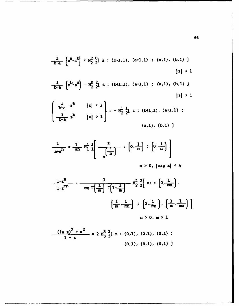
66

IE- (a~b) =H2 0[ z : (b+1,1), (a+1,1) ; (a,l), (b,1)J

l < 1

1(ba) 2C~ z : (b+1,1), (a+1,1) ; (a,1), (b,1)J

IZI >1

b 1 aza Izi < 1

b 1a zb lI >1 -1 12 (b+1,1), (a+1,1)

1 1 H: 1o~ ;1 (oi'J

a+zn L ( -

ni > 0, m > 1

(In z) 2 2 H3 3[ z : (0,1), (0,1), (0,1);1 +z233

(0,1), (0,1), (0,1)]

67

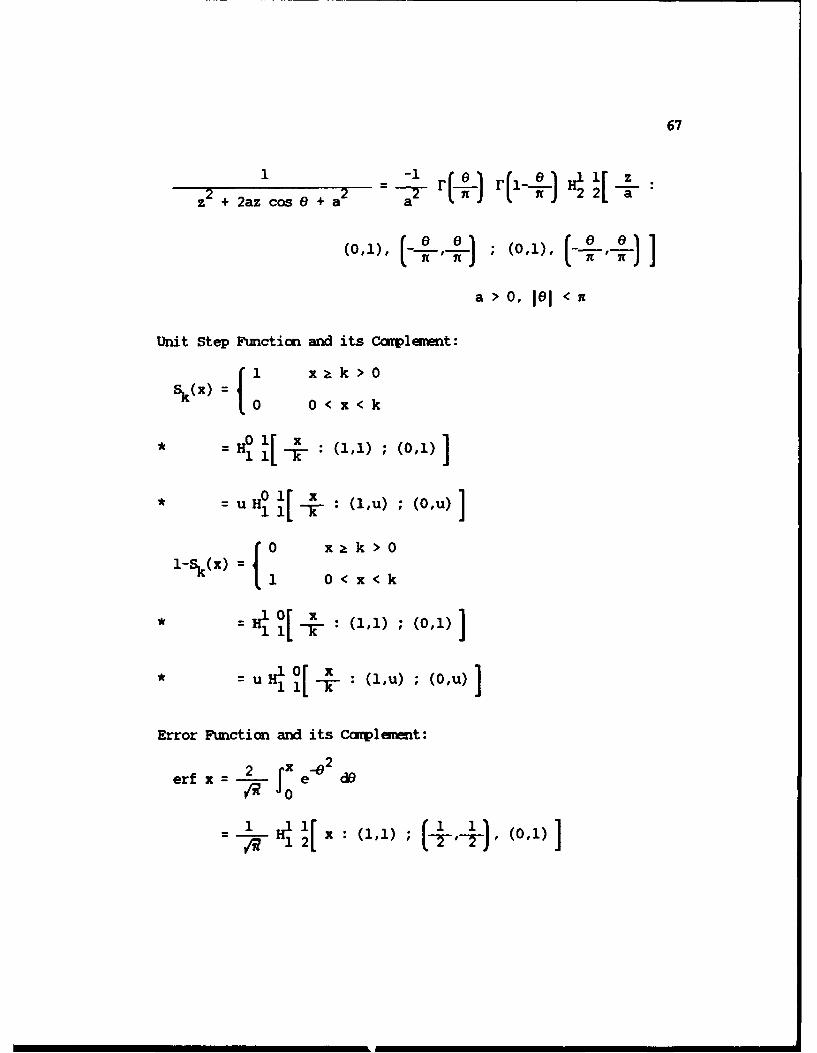
z2 + 2az cos 0 + a2 nr F 2 a

a > 0, ii < it

Unit Step Function and its Complement:1 x ak>O0

Sk(x) =< <0 Or x 1

H =H 1 - : (1,1) ; (0,1)

* =Hu 1 [ - (1,u) ; (0,u)

0 xak>01-k(x) =

= 0< x<k

* - u y : (,u) ; (0,u)

Error Function and its Complement:

erf 2 x e0 2 derfx "0

- H .' 1 , x+ 1 ,o0,11 2 1-l

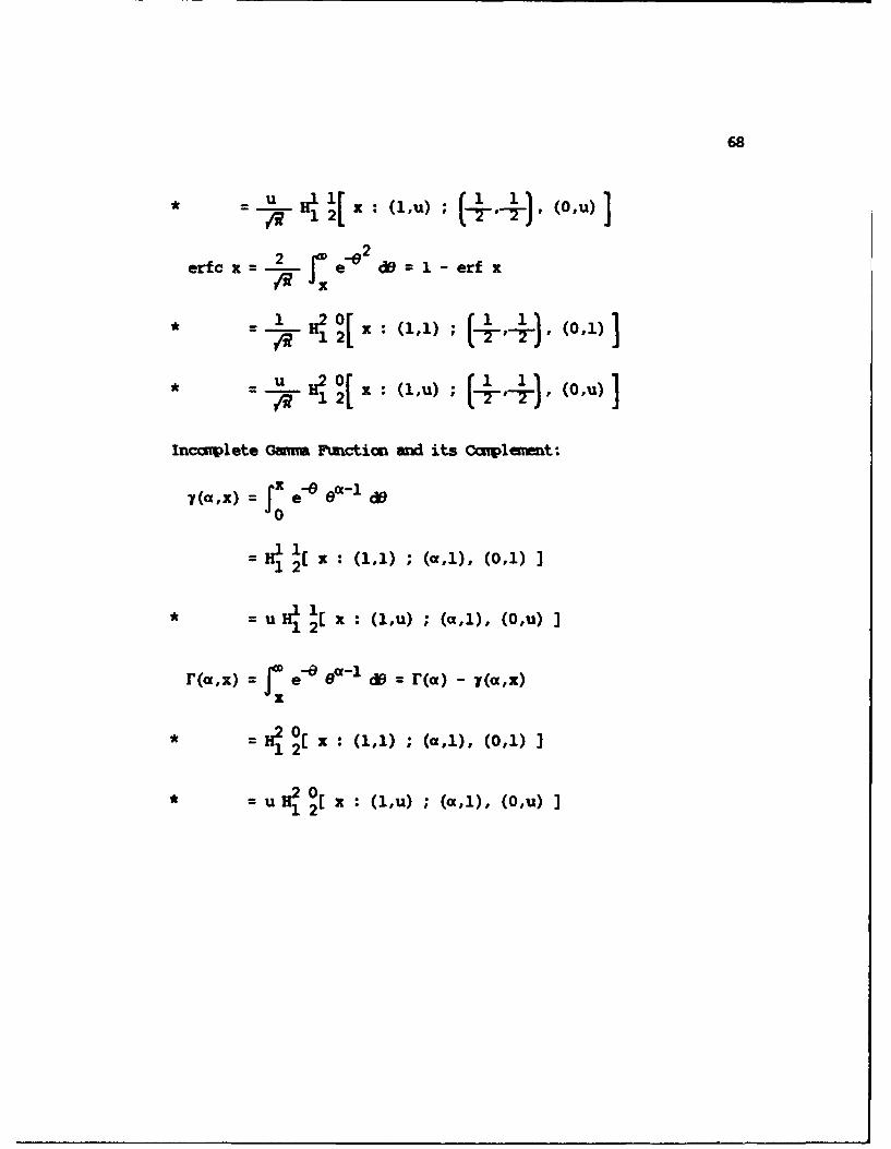
68

*~ -l 1 x Ij: (1,u) ;(O,U)]

erfc x =do ~1 -erf x

=* H x : (11); (o-- i (, 1)1Vq1 2L

u =2 H o[r x : (1,u) ;(0,U)]

Inccmplete Gamu Function and its Carpleent:

10

* = H [ (1,) ; (,), (0,) ]1 2

r(a,x) =re~ el 8 =- d () r ()x

* ~ ~ H. i20 x : (1,U) ; (a,1), (0,U)J1 2

69

Inomplete Beta Functionx and its Coumplemenit:

r (p) H12 12 x : 11,(cx+P') ; (a"1)' (0,1) 1

u, r~)41 x : (1,U), (axP,1) ; (a,1), (0,u) ]

* = F(p) H2 0[ x : (1,1), (cx+p,1) ; (a,1), (0,1) J2 2

u 2 2~) 0 x : (1,u), (a+P,1) ; (a,1), (O,u) J

Trigcnmeitric and Hyperbolic Functionas and their Inverses:

sin z = 2 ; 44 . o-j

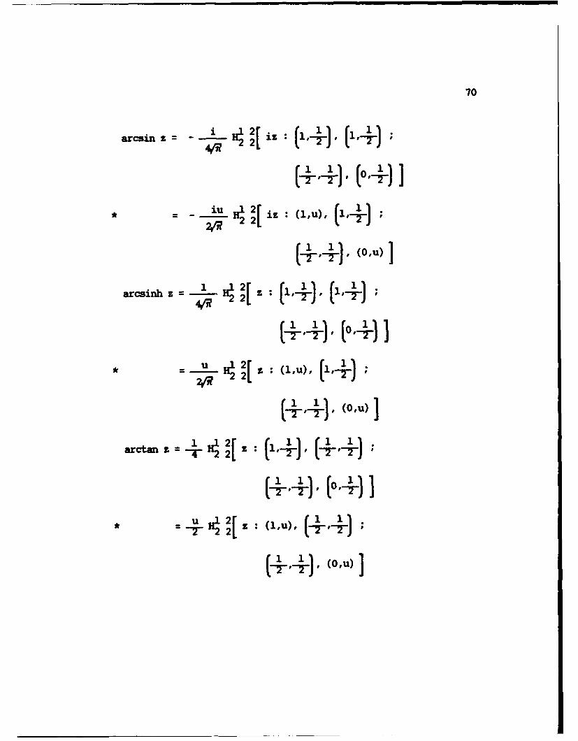
70

arcsin z i 2[. i~ tiz : ~ (~

* = 1~~u Hl 2[ iz : (,)

- 2n

arcinh z 2[1

1(01)]

*+ I (1,u))

(0,u

71

iu4 2 :z (11,u

u z(u) ]

72

e-b cs (z) x H 4/ z:

-bz 0a~ z=fH4'Tz ['i-. H

esin ( z)1 'r 2a / b =i,' x if,(,)

Logarirctan f c I~s

lnz cos 0z ac1n

e7~~~ >1)x +

73

_U2 0[z : (1,u), (1,U) ; (0,u), (O,u)]{~ 0< z IU2 2Cz :(1,u), (1,U) ; (0,u), (0,u)]

z >

In* 1z = u 4 2E z : (lu1), (1,1) ; (1,1), (0,)J

in = U~ 4 2 z : (0,1), (1,1) ;(0,1), (0,1)J

* ~ ~ 4 u H [~ z : (0,1), (1,u) ; (0,u), (0,1) ]

74

UK H: 1[

,o~~H 2[+ ] z [ -(, (,1,,(I)

in (I. + 2z coo zz (,) (1,

+ -,1- .o ); (1,1), (0,1), o,,, J ]

*up H3 2[ z :(1,u), (1',),

Bessel F~s,.tion:

Ova-, --. R -;9[- (. (1, 1 ( 0 ,U, ]

,,,,-,-4 g:[ , [(1,,+, (-+ 4]

75

V Vr+1

JvU(z) = H10 OE z (0D1), (-vu) ]

(Maitland's generalized Bessel functioni)

Hypergeamitric Fuhnctions:

M(a,b,-z) = , (a;b;-z)

r(a) 2

(Confluent Hypegeamn-tric functioni)

2F, (a~~c;-z) r(c) 2(a~b~c;r) = (b) 24 ( 1 a, ) 1 b 1

(Hypegecmric function)

'r (bj)

for p : q or for Pq.1 and IZj < 1

(Generalized HypergecmagtriC fiMCtios)

76

S[{(ai,,A)f{(b.,.B)};-z]- z : (-aiAh))

(, aitland's or Wright's Generalized Hyperg tric function)

MacRobert' E-Fucticn:

E(p; {a1}; q; {bj}; z) = HqP+1 1[ z : (1,), f{(bj#,Bj)

Meijer's 0-Function:

n[ z ([ai)) (=)) C[ z : {(a ii)) ' (( bj1)1)

* 2.6. 9JICKU S R A BRflICTE BlZM

For saie of the special cases of the H-function listed

above, the H-fumction represents the special case only for

certain values of the variable z. For other values of the

variable, the H-ftmction takes the value zero. These cases c

be identified by a restriction n the variable such as IzI < 1.

These restrictions arise from the convergence conditions

for the H-function given earlier. These H-functins are of

77

Convergence Type VI which neans they can be evaluated by the1sum of IHP residues for zj <1 and by the negative sum of

> -!-. But the H' 0 and H 2 0 classes ofP residues for z > 1 22

H-functions have no IP poles so the value of the negative sum

Iof IMP residues is zero. Therefore, H(z)=O for IzI >-CF-.

Sinlarly, the 1 a 12 2 classes of H-fumctions have no LHP

poles so the value of the sum of 1IP residues is zero.1

Therefore, H(z)=0 for Izi < -

Through scaling the variable with the parnmeter c, it is

possible to change the value where the H-function changes from

representing the special case to taking the value zero. For

exauple, an H1 0 H-function can exactly represent the power

function zb for Izi < M where M is any finite positive

costant. Provided M is finite, 14 nay be as large as desired.

Similarly, an l 0 H-function can exactly represent the same

power function zb for Izi > c where e>0 nay be as umall as

desired. These scaled H-function representations (given

earlier in the list of special cases) allow a nearly ccuplete

representation of the special cases.

Another way to avoid this limitation of Convergence Type

VI H-functions is to allow a slightly different function to be

represented for certain values of the variable. The method

basically involves introducing poles into the other half plane

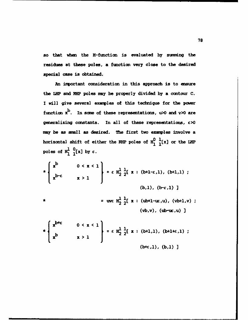
78

so that when the H-function is evaluated by summing the

residues at these poles, a function very close to the desired

special case is obtained.

An inportant consideration in this approach is to ensure

the IEP and 1IP poles nay be properly divided by a contour C.

I will give several exanples of this technique for the power

function xb . In some of these representations, u>O and v>O are

generalizing constants. In all of these representations, c>O

nay be as small as desired. The first two exaiples involve a

horizontal shift of either the RHP poles of H [x or the LMP

poles of 0 [xJ by e.

* 1 -E X > 1 j = £ H~ [ x : (b+l-c,l), (b+1,1)

(b,l), (b-cj)

- uv 14 1[ x : (ub+l-xw,u), (vb+l,v)

(vb,v), (ub-w,u) J

( xk ~ 0 0 x < 1) -1

* ~j= '2 [ x : (b+1,1), (b+l+c,l)b xb> l

(b+c,l), (b,l)]

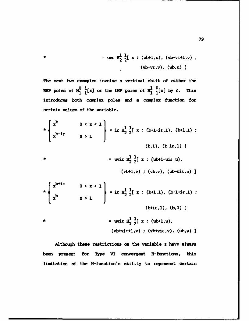
79

* = uvE 4~ x : (ub~1,u), (vb+vw+1,v)

(vb+vc,v), (ub,u) ]

The next two exmples involve a vertical shift of either the

JIW poles of [1 1 x] or the IP poles of 1 [x]~ by c. This

introduces both caplex poles and a complex function for

certain values of the variable.

* 1 - x > 1 = ic H [ 1 x : (b+l-iE,l), (b+1,1)

(b,1), (b-ic,i) I

* - ui. H x : (ub+1-uiC,u),

(vb+l,v) ; (vb,v), (ub-uic,u) ]

* [ x : (b+1,1), (b+l+ic,l)xb x >1

(b+ic,l), (b,l)]

* = uvic 14 1[ x : (ub+l,u),

(vb+vic+l,v) ; (vb+vic,v), (ub,u) ]

Although these restrictions on the variable z have always

been present for Type VI convergent H-functions, this

limitation of the H-function's ability to represent certain

80

functions over all values of the variable was only recently

discovered. The practical mnthods suggested above to nmnindze

the inmpact of this limtation through scaling, a slightly

different function, or use of caplex paraneters are also newly

developed.

* 2.7. U F M H-PUNCrlC! AM INFINITE SUMBILITr

For a function of a real variable, f(x), which is nonzero

only for positive values of the variable, the rth nment about

the origin of f(z) is given by

Pr xrf(x) dx (2.69)0

provided the integral in Eq (2.69) exists. If f(x) can be

represented as an H-famction, it is often easier to find the

rth marent of f(x) using the Mellin transform formla

Pr = Ar+[f(x)] (2.70)

In particular, if

f(X) = q cx : {tai,Ai)) ; {(bj,Bj)) (2.71)Su i=l,...,p j=2,

6q

then using Eq (2.68),

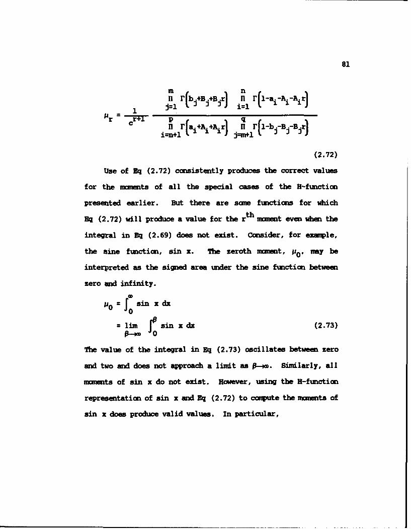
81

1 j=j (b i i=1 •

.a+B-b -B .-B r.irn+l (aj-ir l (1 j jj

(2.72)

Use of Eq (2.72) consistently produces the correct values

for the numnts of all the special cases of the H-functiom

presented earlier. But there are same functions for which

Eq (2.72) will produce a value for the rth moment even when the

integral in Eq (2.69) does not exist. Consider, for exmple,

the sine function, sin x. The zeroth mmmt, y' my be

interpreted as the signed area under the sine function between

zero and infinity.

= 0 sin x dx"0

= lim r sin x dx (2.73)P--mD 0

The value of the integral in Eq (2.73) oscillates between zero

and two and does not approach a limat as a--4m. Similarly, all

mumonts of sin x do not exist. However, using the M-function

representation of sin x and Eq (2.72) to cavpute the naents of

sin x does produce valid values. In particular,

82

Pr 4rl ri4r)

rr= (-1T r! r an even integer (2.74)

0 r an odd integer

This apparent contradiction can be resolved with the

concept of infinite sumbility of integrals. A thorough

discussion of infinite sumbility is beyond the scope of this

thesis, but a brief introduction to the concept through

infinite sums will be given. Eder began the study of this

topic by considering the value of the infinite sua (- 1 )i-

_n i-IThe limit of partial sums n -i =(-1) does not exist, since

i=1Snl if n is odd and SnO if n is even. Euler believed the

infinite sum should have the value 1 since it is the limit of

the average of the partial sums an = - S whether n is odd

or even.

Since Euler's tim, Cesiro and Holder have developed well-

accepted schemes to find the values of infinite sum Whose

partial sum do not converge to a limit. 8l1der's shems are

based on the averages of the partial sums (H-i), the averages

83

of those averages (H-2), etc. Ceskro's schemes (C-1, C-2,

etc.) are less intuitive and slightly more caplicated. The

approach described in the previous paragraph defines both the

C-1 and H-1 schemes, which are identical at the first level.

It is important to recognize that if an infinite sum does

converge, any of the smmiwbility schemes will produce the sam

result. Similarly, an infinite sum which is C-m (H-rm) sumable

will produce the same result using the C-n (H-n) scheme where

n>m.

There is a direct analog to this approach for integrals

over an infinite range. An integral which does not exist may

still be summable under a sumbility scheme. The zeroth

nment of the sine function is an example of such an integral.

Under the C-1 or H-1 sumnability schemes for integrals, the

integral for the zeroth moment of the sine function takes the

value umity, the some as that produced with Eq (2.72).

There are several functions for which Eq (2.72) will

produce a value for the rth mflent even when the integral in

Eq (2.69) does not exist. In this case, however, Eq (2.72)

always produces the "correct" value under an appropriate

summbility scheme. It is as though the H-fumction knows about

infinite sumubility and uses it correctly when it is

appropriate to do so. The first few nents of some

84

trigonouetric and hyperbolic functions are given in Table 3

below. Although the integrals for these mments as in

Eq (2.69) do not exist, these values are widely accepted as

"correct."

Table 3. Monts of Triagonmetric and Hvnerbolic Fumctics

ment Rim I Cos _ sinh x cmh x

Zeroth 1 0 -1 0

First 0 -1 0 1

Second -2 0 -2 0

Third 0 6 0 6

Fourth 24 0 -24 0

Fifth 0 -120 0 120

2.8. EVAU3ATICt OF THE H-F IOK

Like most contour integrals in the conplex plane, the H-

function is usually evaluated by summg the residues at the

poles of the integrand. The contour C, which is sametines

referred to as the Branuich path, is connected to a semi-

circular arc to create a Branmdch contour, a closed curve in

the complex plane. By the residue theoren, the value of the

integral around the closed Brcmuich contour in the positive

(counter-clokwise) direction is the sum of the residues at the

poles enclosed by the contour. Under very general conditions,

85

the contribution of the sem-circular arc vanishes as the

radius increases without bound. In this case, the desired

integral over the Bromich path C equals the integral around

the closed Braiwich contour, the sun of residues at the poles

interior to the closed contour.

Since the Bramwich path C (by definition) divides the LiIP

and MW poles of the integrand of the H-function, connecting a

semi-circular arc to the left will enclose all the IMP poles of

the integrand as the radius increases without bound.

Travelling around this Bronuich contour in the positive

(counter-clockwise) direction, we cover the Bromwich path C in

the desired direction fran w-im to w+iw. Under the general

conditions referred to earlier, the desired integral along the

Braowich path C equals the sum of residues at the IHP poles.

Conversely, connecting to C a semi-circular arc to the

right will enclose all IW poles of the integrand as the radius

increases without bound. Travelling around this Browich

contour in the positive (counter-clockwise) direction, we cover

the Brcmwich path C in the opposite of the desired direction

frm w-im to w+im. Changing the direction travelled around the

contour frm counter-clockwise to clockwise sinply reverses the

sign of the integral. Under the general conditions referred to

earlier, the desired integral along the Brcwich path C from

86

w-im to w+ic equals the negative sum of residues at the lHP

poles.

The convergence conditions given in Section 2.3 take care

of these details and indicate where the H-function may be

evaluated as the sum of LHP residues or the negative sum of NIP

residues. Depending on the pattern of the poles of the

integrard, the process will result in a finite or infinite

series. For all of the special cases listed above, this

evaluation method will produce a series which equals the Taylor

series expansion of the special case.

While it is possible to verify the H-function

representations of the special cases in this manner, it is

often difficult and tedious to produce the series, especially

with poles of multiple orders. Eldred [1979] wrote a computer

progran to evaluate the H-function by suning the residues at

the appropriate poles. Cook [1981; Cook and Barnes, 1981]

improved the progran and added extra capabilities dealing with

algebraic cmbinations of independet H-function variates.

Still, Cook's progran will evaluate a general H-fumction over a

specified range (and with a specified interval) of the real

variable x when the parameters are input.

CHIAT 3

THE H-PUICIK DISTRIBUTICN

3. 1. DW INITICN

Because the H-fumction in Eq (2.1) can exactly represent

the kernel of wnmy camon probability density functions, it was

natural to define an H-function distribution as the product of

an H-function and a constant, k, which normalizes the area

under the H-function (over the appropriate range) to unity. An

H-function variate has the following probability density

function (p.d.f.) [Carter, 1972; Carter and Springer, 1977,

pp. 545-546; Springer, 1979, p. 200]:

f(x) = "=...,p jl,...,qI

0 otherwise

(3.1)

In this case, the random variable X is called an H-function

variate which follows an H-function probability law or H-

function distribution.

Use of an H-function representation as in Eq (3.1) for a

87

88

probability distribution has several advantages. First, it

unifies nearly all cammon continuous probability distributions

of positive random variables under one very general class of

functions. The many named distributional forms which arise

naturally in common problems in probability my be nnaged with

only one function, the H-function. The H-function can also

represent an infinite number of other, unnamed distributional

forms.

The H-function also eliminates the need to specify the

range of the random variable for which the density is nonzero.

The H-function exactly represents the desired density over the

appropriate range and is zero elsewhere.

Many characteristics of a probability distribution such as

the moments about the origin, the cumulative distribution

function, and the Laplace, Fourier, or Mellin transform are

easily found frm the H-function representation. Finally, if

new random variables are defined by algebraic combinations of

independent H-function variates, the densities of the new

random variables are easily obtained.

3.2. MO(DTS XF WZ P NrICH DISTRIBUTION

For the real random variable X with p.d.f. f(x) which is

nonzero only for positive values of the variable, the rth

moment about the origin of f(x) is given by

89

r f x f(x) dx (3.2)

provided the integral in Eq (3.2) exists. If the density f(x)

can be represented as an H-functicn, it is often easier to find

the r moment of f(x) using the Mellin transform formula

Pr = A r+llf(x) ] (3.3)

In particular, if

f(x) =kpmnF cx : ffa.,Ai) ; ffb.,Bj)) (3.4)p= ...,p j=l,...,q

as in Eq (3.1) then using Eq (2.68) [Carter, 1972; Carter and

Springer, 1977, pp. 546-547; Springer, 1979, pp. 201-202],

m n

C nr rai+Ai+Air) j irll -b j-BB jri--n+1 "lxjjml[ 333

(3.5)

Eq (3.5) is very useful in finding the mmnents of all H-

function variates, including all of the special cases listed in

Section 3.5.

3.3. MMIJMIK -W THE H-PUNMOIN DISTRIBLYTIC ONS

Cook [1981, p. 109; Cook and Barnes, 1991] gave a

practical method to determine the normalizing constant, k, for

90

the H-fnmction distribution. If the integrand of e n[cx] hasp q

no pole or zero at s=1, then since the zeroth moment of a valid

statistical distribution mst be tuity,

k 1 _ 1

using~~ qq (3s)wih

p qq

H r a.+A. jH rf1-b.--bi--n+l ] --m+1 ]j)

=Cmnr l Ir(bj+Bj) i r(1-ai-Ai)

(3.6)

using , (3.5) wth r1or.Th odtion that the integan of n [cx] has no pole

at s=1 coe from the need to evaluate the Hellin transform at

S=l. A commonly met condition of nearly all H-function

-b.distributions which guarantees no pole at s=1 is that B < 1

for j=l,...,m and -Ia > 1 for i=l,...,n. For the firstA.

order H-fumction H0 0[cxj, Jacobs [1986, p. 46] noted that this0 1

restriction corresponds to the region in his (B,b) plot [p. 53]

above the line b=-B. He also shows [pp. 71-72] that first

order H-function distributions in this region are uniquely

determined by their moments.

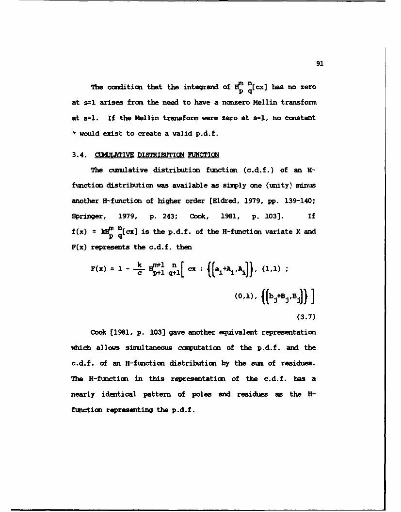
91

The condition that the integrand of lp q[cx] has no zerop q

at s=1 arises from the need to have a nonzero Mellin transform

at s=1. If the Mellin transform were zero at s=1, no constant

7- would exist to create a valid p.d.f.

3.4. C( JLATIVE DISTRIBUTION FUNCTICT

The cumulative distribution function (c.d.f.) of an H-

function distribution was available as simply one (unity) minus

another H-function of higher order [Eldred, 1979, pp. 139-140;

Springer, 1979, P. 243; Cook, 1981, p. 103]. If

f(x) = kip n[cx] is the p.d.f. of the H-function variate X andp q

F(x) represents the c.d.f. then

F(x) = 1- - - 1 q+l cx: (ai+Ai,Ai), (1,1) ;

(3.7)

Cook [1981, p. 103) gave another equivalent representation

which allows sinultaneous computation of the p.d.f. and the

c.d.f. of an H-function distribution by the sum of residues.

The H-function in this representation of the c.d.f. has a

nearly identical pattern of poles and residues as the H-

function representing the p.d.f.

92

F() = 1 - k x n r cx : ffa. AJI, (0,1)p+1 q+1l A 1 J

(3.8)

Cook [1981, p. 104] also showed that the c.d.f. (in

addition to the ccmplementary c.d.f.) was an H-function. In

particular,

__L dn n+1 cx : (1,1), 14 ai+A.,Ai);

F(x) f Bpj),(,)1

=

-k H~p*l n r cx: (1,1)- - 1 q l cx : j ai+Ai , A ), (i,i) ;

(3.9)

where I is as given in Eq (2.62).

It is possible to introduce an arbitrary, positive

generalizing constant, u, to Eq (3.9). The new generalized

formula for the H-function representation of the c.d.f. of an

H-function variate is

93

c- I+1 q+l[ x : (1,u), uai+AiAi ;

* (x) = u ~ Bfjl 0U =

-uk- q+l cx: ffai+Ai, Aj), (1,u) ;

(3.10)

where I is as given in Eq (2.62) and u>O is arbitrary.

3.5. SPECIAL CP.SES - STATISTI(ML DISTRIBUTIOIS

With the parameters given below, the H-fumction

distribution can represent all of the following probability

density functions as a special case [Carter, 1972; Carter and

Springer, 1977, pp. 547-549; Mathai and Saxena, 1978, pp. 10-

12; Eldred, 1979, pp. 104-108; Springer, 1979, pp. 202-207;

Cook, 1981, pp. 85-87; Cook and Barnes, 1981, p. 300;

Bodenschatz and Boedigheimer, 1983, pp. 17-22; Bodenschatz et

al, 1990]. The H-function representations of the cumulative

distribution functions and a fonuila for the moments about the

origin are also presented. In some of the representations, v

denotes an arbitrary positive constant. In the c.d.f.

representations, u denotes an arbitrary positive constant.

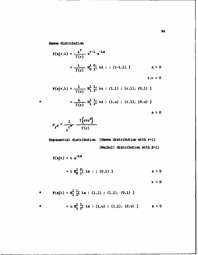
94

Gamma distribution

f(xlr,A) - (r) xr-I e_)x

X~ Cx : ; (r-1,1) I x>O0F(r)

r,X > 0

F ~ (r)A 1 12

rU H1. 1[ Xx : (1,u) ; (r,1), (o,u) JT(r) 1

z>O

1 r(r+r*j

r* r r(r)

Exponential distribution (Gamma distribution with r=1)

(Weibull distribution with P=1)

f (xPl) = e7•-I

1>0

* F(xl X ) H1 1[ x : (1,1) ; (1,1), (0,1) ]1 2

U ux[ XX: (1,u) ; (1,1), (0,u) x > 02

95

1 r (l+r)

Chi-Square distribution

(Gums distributiu with r an 1

f(xO) = x e

2 F x]

x>O1-y I' > 0

F'"xj P) + ,, K[+ ,, , 1. (o.,

H [, 1., (1,u) 1) (0,u)]

x>O

r Ir

weibull1 distributim~

f(XjPAX) = P I X(P-1) e * r

,x > 0

*= U4 1~ x z : (1,u) I (0,u)

11

pr r r(++

Rayleigh distribution (Weibull distribution with P=2)

f (xjl) A 2 x e _Xi

1>0

97

* :° H [.: I T°(1,u) ; i1. .1 o

1

r r r(1+±)

Maxwell distribution

e>0

* ( , ,r x 2: (1 , ; x (o>, l

0>O

_~lg 2

,r , r r .,+

98

Hal f-Nornmal distribution

f(xo) 2 e

a 1o[2.1o/70 10>0

- H-U 1 x (1,u) ;(~ ) (Oiu)]

x>Or

Beta distribution of the first kind

Sr(a+p) x(a-1) (1 -x)(P -1) o < x < 1r (a) r (p)

- (cl+P) H. 0[r(a)

alp > 0

F~xjar)a= ) 1 2[ : (1,1), (a+ ,1) ;]F(xla,) r(a) [

(all), (0,1)]

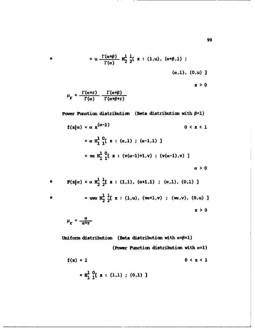
99

* = ~U r(a*p) 4 1[ : amu, (cxep,1);

(all), (Olu)]

r(a+r) '(cx+p)r r(a) r(a+p+r)

Power Function distribution (Beta distribution with P=I)

f(xla) = a 1(a-l) 0 < x <

= a 1i 0( x : (all) ; (a-1,1)]

= Va I 0[ x :(v(a-1)+1,v) ; (va-1),v) I

> >0

* F(xla) = a H 1[ x al(l,), (a+1,1l) ; (al1), (0,1)

* = ~uw H4 1[ x : (1UM' (wa+1,v) ; NUMv, (0,u) J

Uniform distribution (Bet& distribution with auP31)

(power Function distribution with a=l)

f(z) = 1 0 < x<1

100

= V 0 x : (1,v) ; (Ov)]

F (X) = 14 [ x : (1,1), (2,1) ; (1,1), (0,1)j

* ~ U = 1[4~ x : (1,U), (v+1,v) ;(v,v), (0,u)]

x > 0

Pareto distributicn

f(xla) =a X-W)x >1

= a H0 1[ x : (-a,1) ;(u1111

0 1= va Hi1 [i x :(1-v(cx+1),v) ;(-v(a+1),v)]

a > 0

* F(xia) =a 02

*= *va 0 2[x -uv (,)

x > 0

a for a>r

Hal f-Cauchy distributiai

20f ( z I O) = x [ 2 + e

101

6>0

* F(x) 2 x (1,1),

- 2[ x (1,u),

R I) I(0,u)]

x>O

F + +) rif r is even~PJr = I

do not exist if r is odd

Hal f-Sttlent distribution

_x2 2

f~~xIL) ~ -4 (1 _________ _______

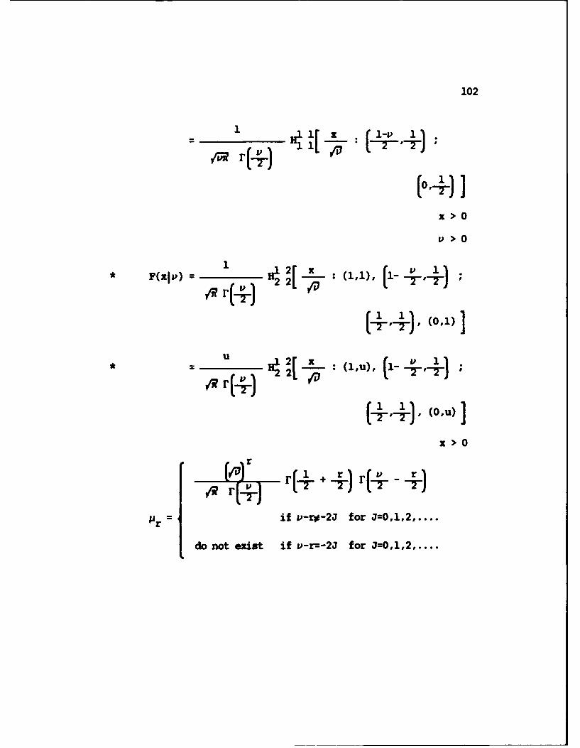
102

1

x>O

Hl 1 XM'>

(01+ ) ]

u 2[ux

x>O

r[+

r = if P-r-2J for J=0,1,2,....

do not exist if P-r=-2J for J=0,1,2,....

103

F distributimr

f~~xfrsa)f I f(2L w~-- (~If(~ r+)I

qV- LTJW JJ4

xa > 0

F~~r(± r(+) 2 v

*~~~2 ________ (1,u),

r f v r f l 1 20

104

r

if w-r*-J for J=0,1,2,....

do not exist if w4 -r-J for J-0,1,2,...

Beta distributioni of the second kind

f(xla,P) -w I rPXp (u-i)

a F ca ) r ( )

x> 0

* F(xla,p) 1 ~x Hl 2[ X : (1,), (1-P,1);

(all), (0,u)]

> 0

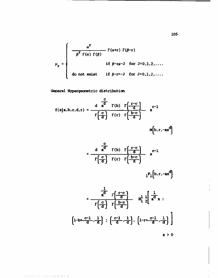
105

r

pr d) () r(a+r) r(p-r)

p r = I if P-r*-J for J=0,1,2,..

do not exist if P-r--J for J=0,1,2,..

General Hypergeczetric dlistributixi

d a r(b) r f~~ C-1f(xla,b,c,d,r) P -X

rM (r) r -

m(bir,-axl

c

d a r(b) rlr C-1

FPr)

Flbir,-aA)

11

aT>x

106

* F(xja,b,c.d,r) =--- 42 TX______

(1,1)( C 1)

-uI * - CT[.'.

0-.A, ri-b. C 1

x > 0

r-4 - r (r- a

if --- -dr-*-Jfor J=0,1,2,...

do b-o=- for J=0,1,2,...

107

It should be noted that since the H-function distribution

is only defined over positive values, symmetric and doubly

infinite distributions like the normal and Student's t must be

manipulated in their folded forms. While the normal, Student's

t, and Cauchy distributions are not special cases of the H-

function, their folded forms, the half-normal, half-

Student's t, and half-Cauchy, are representable as H-function

distributions.

The ven diagram in Figure 1 shows the relationship

between many common first and second order H-function

distributions. The Erlang distribution is simply a gamm

distribution with an integer shape parameter r. The

exponential distribution is a proper subset of both the Weibull

distribution and the Erlang distribution, which is a proper

subset of the gama distribution. one exponential distribution

(with X-=) is a special case of the Chi-Square distribution,

which is also a proper subset of the gwmsa distribution. If a

Chi-Square distribution has an even number of degrees of

freedom, P, it is also an Erlang distribution with 1. The

Rayleigh distribution is a proper subset of the Weibull

distribution. All of these named distributions, plus the Half-

Normal and Maxwell distributions, are special cases of the

f class of H-function distributions.

108

Rayleigh

Maxwell

Weibull 1001

H-Functions,

H-Funct ions

0 o

H,1

109

It is well known that the Uniform distribution is a

special case of the Power Fumction distribution, which is a

special case of the Beta distribution. All of these

distributions are represented as H' 0 H-function distributions.1 1 Hfnto

Further, it was shown in Section 2.4.6 that the 1 cs0 cla of

H-functions is a proper subset of the H 0 class of H-

functions. Therefore, all of the namd distributions in

Figure 1 can be exactly represented as H-function distributions

in the 0class.

An H-function representation has not been given for the

p.d.f. of the Lognormal or Logistic distributions. Conversely,

no one has proven that these distributions cannot be

represented as H-functions. This is an area for future

research.

* 3.6. BITRAR_ RG F T Y H-i TIC VARIATES

The H-functions in same of the p.d.f. representations in

Section 3.5 are Type VI convergent according to Table 1 in

Section 2.3. Consequently, they represent the desired p.d.f.

over a certain range of the variable and, since they lack poles

in the opposite half-plane, are zero for other values of the

variable.

Specifically, the H-function representations of the Beta

(first kind), Power Fumction, and Uniform distributions above

110

are all 1 j01 1 Type VI convergent H-functions with no NIP poles.

As listed above, they represent the desired p.d.f. over

0 < x < 1 and are zero for x > 1.

Similarly, the H-function representation of the Pareto

ist1above is an 1 Type VI covergent H-functindistribution 1

with no [HP poles. As listed, it represents the Pareto p.d.f.

for x > 1 and is zero over 0 < x < 1.

This limitation (as discussed in Section 2.6) of the H-

function to represent a general power function or beta-type

function for all x > 0 is actually an advantage when

representing the statistical distributions. Using the H-

fumction representation eliminates the need to specify the

range of the variable for which the density is nonzero. The H-

function representation gives the desired p.d.f. for the

appropriate range of the variable and is autcmuatically zero

otherwise.

The newly discovered technique of scaling these Type VI

convergent H-functions discussed in Section 2.6 is also

applicable here. By changing the value of c in the definition

of the H-function, it is possible to alter the point at which

the H-function changes from representing the special case to

taking the value zero. For the statistical distributions

mntioned earlier, this allows more flexibility in representing

ill

the same functional form over a more general range. Given

below are the new H-function representations of the densities

for the Three-Parameter Beta distribution, the Power Function

distribution over (0,M), the Uniform distribution over (0,M),

and the Pareto distribution over (e,m). In some of the

representations, v denotes an arbitrary positive constant.

Tbree-Parameter Beta distribution of the first kind

f~l,,)= r(a+p) 1 x (a-1) (M-x)(P-1)f(xla 'M4) = r( a) r1()

O<x<14

= - r(a+P) H11 [ x (cx+-1,1) ; (a-1,1)]m r(a) I -

a,p,M > 0

Power Function distribution over (0,M)

(Three-Parwmeter Beta distribution with P=i)

f(xla,m) =a 1 x (a-) 0 < x < 14

* - .- _-- HL[ : (vx-1)+1,v) V (v~U-1),v) ]a,M > 0

112

Uniform distribution over (0,M)

(Three-Parameter Beta distribution with a==l)

(Power Function distribution over (0,M) with a=1)

f(xIM) = 1 0< x<M

v v O x. (1, V) (0 (OV)] 1> 0

Pareto distribution over (c,w)

f(xia,c) a e x-( + )

vu H. 1 (1-v(a+l),v) ; (-v(a+l),v)

a,E > 0

3.7. TRADMEMMTKqZNS Qr INEEN H- I(MO VAIATES

A significant advantage of using the H-function

representations of statistical distributions is that they make

finding the distribution of an algebraic combination of

indepe nt random variables much easier. Carter [1972; Carter

and Springer, 1977, pp. 549-557; Springer, 1979, pp. 207-219]

showed that the product, quotient, or power of indepe t H-

function variates thmselves had an H-function distribution.

113

In fact, the resulting density of the new randam variable can

immediately be written (as an H-function) using only the

parameters of the H-functions in the algebraic combination.

Springer [1979, pp. 217-219] described a nethod for

finding the H-function distribution of an algebraic ccntination

(including constants, products, quotients, and powers) of

independent H-function variates. Cook [1981, p. 92] combined

the three theorem of Carter [1972; Carter and Springer, 1977,

pp. 549-557; Springer, 1979, pp. 207-217] into one very

complicated theorem. Using Cook's theorem, the H-function

P.V ]distribution of Y = I X is immediately available, where X.,

j=1 i j

j=1,... ,V are mutually independent H-function variates and Pj,

j=,...,V nay be positive or negative. Carter's separate

results are given below, not Cook's combined results.

3.7.1I. DISTRIBUTION OF A 8C9

If Xi, X2 ,..., XN are mutually independent H-function

variates with densities f 1 (xl), f 2 (x 2 )o..., fN(xN),

respectively, where

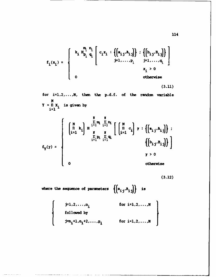
114

k cixz: {(aijNij)} ; {(b1i 1Bij)}

K. > 0

0 otherwise

(3.11)

for i=1,2,...,N, then the p.d.f. of the randcun variable

NYf=X. is given by

N N

fy(y) == I~j ijji A

y >O

0 otherwise

(3.12)

were the sequnce of parameters {(a~i Aj)} is

j~lo,# .. Pnifor il,2,...,N

j~nil~ni2,..,pifor i=1,2,...,N

115

and the sequence of parameters fbjB )I is

j=,2, ... ,mi for i=1,2,...,N

followed by

j-j+in +2,..., for i=1,2,..... IIn effect, the formula retains the gam terms in their

previous place (numerator or denominator) in the integrand of

the H-function.

3.7.2. DISTRIBUTI.- 0!_ A aWIET

If X and X are independent H-function variates with

densities f 1 (zl) and f 2 (x2), respectively, where

= k i cix, : (ajA) ; bjj)fi (xi) :j ,. "'i j-l,... j'qi

z. > 0

0 otherwise

(3.13)

for i=1,2 then the p.d.f. of the randan variable Y - is

given by

116

klk 2 m14T12 n, "r2 r l

22 HPq2 ql+P2 Ic 2 Y (AI MJJ

fy(r) - c2 (eE)}]

y > 00 othrwise

(3.14)

where the sequence of parameters {(dD)} is

and the sequence of paruiwters{( )}i

117

{(bln 10 l+)...(blql 1j

(1- a22+1 -2A 2n2 1, An+1 . 2- A 2 , A1,2) }3.7.3. DISTRIBUTION X_ A A V T O

If X is an H-functim variate with density f(x) where

k~x C t : x : ((ai'Ai)) ; {(bi:Bj)]}J 1>0f(x) =I i=l,...,p j=l,...,qI

0 otherwise

(3.15)

pthen the p.d.f. of the randcm variable Y = X is given by

118

P-i mn[ Pk c HPq I y: l(a-AiP+A.,A.PM

i=1,I...Al

j=l, ... 1q

0 otherwise

(3.16)

when P > 0 and

P-I n[ Pk c Hq p1 c Y : ttlbj +BjiP-BiBjPJ)j=1.... ,A

-y {()f1-ai+A.P-A,, -A.P)I y >O

0 otherwise

(3.17)

when P < 0.

3.74. USE _W JAeS' (Bb KoT _IN FTIDN PWR

g& FIRST CRM -I ION VARIATES

Even first order H-fumctions (possessing only one gumm

term) can represent a wide variety of distributional forms.

For example, an H-function distribution can have a shape which

is not quite that of either a Weibull density or a gumma

119

density. The plot given in Figure 2 of the (B,b) parameter

space for first order H-function distributins by Jacobs [1986,

p. 53; Jacobs et al, 1987, p. 134] shows the ability of first

order H-functin variates to model an infinite number of other,

unnaied distributional form.

b _Legn

C - Cd-SquareG E - Exponential

1.5 C G-G nMuMG H - Half-NormlG M - Maxwell

1.0 M C R - RayleighW G W - Webull

W G Blank space - an0.5 R C unnamed

W G H-fumctionW 0 distribution

0.0 R K0.5 G W 1.5 2.0 B

G W-0.5 C W

0 W

-1.0

Figure 2. Classical Statistical Distributios M

First Order H-Functi in (B.b)Space

Jacobs [1986, p. 55; Jacobs et al, 1987, p. 144] showed

how the (B,b) plane can be used to determine the H-function

120

distribution of positive powers of H-function variates. Since

Eq (3.16) in Section 3.7.3 for P>O does not change the values

of m, n, p, or q, positive powers of first order H-function

distributions are also first order H-function distributions.

Further, Jacobs noted that all positive powers of the H-

function variate X with parameters (b*,B*) lie on the line in

the (B,b) plane parallel to the line representing the Weibull

family of probability density functions and through the point

(B*,b*).

Jacobs [1986, p. 55; Jacobs et al, 1987, p. 144] gave

three examples of the use of the (B,b) plane in finding the

distribution of the power of H-function variates. He made a

slight error when he stated that the square of a half-normal

randm variable has a Chi-Square distribution. Instead, the

square of a standard (i.e. o=1) half-normal random variable has

a Chi-Square distribution with P=1. He correctly stated that

the square of a Rayleigh random variable has an exponential

distribution and that any positive power of a Weibull random

variable has another, different Weibull distribution.

* In particular, if X has a Rayleigh distribution with

parameter X, then Y=X has an exponential distribution with

parameter X. If X has a Weibull distribution with parameters P

and X, then Y= where P>O has a Weibull distribution with

121

parameters - YO and X. I do not believe these relationships

were coumnly known.

* There are other new relationships between statistical

distributions available from using the (B,b) plane of first

order H-fumction distributions. If X has a half-normal

distribution with paramter o, then Y=X2 has a gumm

1 1distribution with parameters r = and ) = -- r. If X has a

Maxwell distribution with parameter 6, then Y=X2 has a gtea31

distribution with parameters r and -1 If X has a

Maxwell distribution with parsmter e = , then Y=X has a

Cd-Square distribution with parameter P=3. If X has a

Rayleigh distribution with parameter X = 1 , then Y=X2 has a

Chi-Square distribution with parameter P=2. I do not believe

these relationships are cciml y known, either.

* The (B,b) plane is useful for finding the parameters for

powers of first order H-function variates. If P>1, the

parameters for Y=XP can be found by traveling down an inugiary

line toward the lower right of the graph and parallel to the

line representing the Weibull family of densities. If O<P1,

the parameters for Y=X P can be found by traveling up an

imaginary line toward the upper left of the graph and parallel

to the line representing the Weibull fauly of densities. In

122

either case, the parameter B for Y is sinply the product of P

and the parameter B for X.

3.7.5. DISTRIBUTION OF A SLJ4

Ai though the products, quotients, and powers of

independent H-function variates have H-function distributions,

this characteristic does not, in general, extend to sum.

Analogs to Carter's results in Sections 3.7.1, 3.7.2, and 3.7.3

do not currently exist for sums of independent H-function

variates.

Because the Laplace transform of the p.d.f. of an H-

function variate is readily obtained as another H-function, it

was hoped the distribution of a general sum of H-function

variates had an H-function distribution. The Laplace transform

of a density which is nonzero only over positive values can be

used like the moment generating function or characteristic

function. The Laplace transform of the p.d.f. of the sum of

two independent randam variables is the product of the Laplace

transforms of the individual densities. If this product were

available as another H-function, it could be inverted

analytically, yielding the desired density expressed as an H-

function. The problem reduced to determining whether the

product of two H-functions was, in general, another H-function.

Because the H-function can exactly represent nearly every

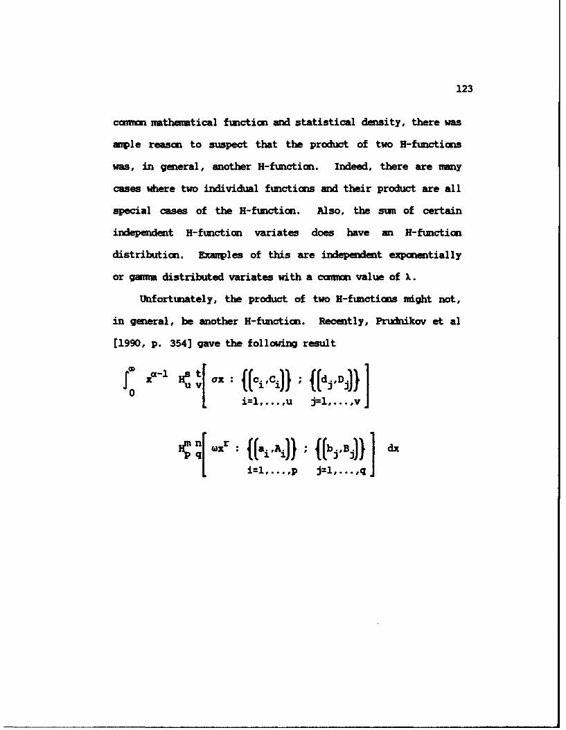
123

cannon mathematical function and statistical density, there was

ample reason to suspect that the product of two H-fumctions

was, in general, another H-functiom. Indeed, there are =mny

cases where two individual functions and their product are all

special cases of the H-functin. Also, the sum of certain

independent H-function variates does have an H-function

distribution. Exanples of this are independent exponentially

or gam distributed variates with a canno value of X.

Unfortunately, the product of two H-functions ight not,

in general, be another H-function. Recently, Prudnikov et al

[1990, p. 354] gave the following result

j0 1a- v4 i-l,...,u J=l,...,v ]Ii=l,...,p j=l,...,qI

124

1 1 et n+s I w Ira A11 ((1-d.-aD.,rDj)),0 ci p+v q~u Oq'JJ

i=l,...,n j=,...,v

i--n+l,... ,p j=1,...,m u

((bjj 13J)(3.18)

j--m l,...,qI

under certain general conditions. Cuvparing the left side of

Eq (3.18) to Eq (1.7), the Mellin transform of the product of

two H-functions is another H-function. Using a result from

Erd6lyi [1954, p. 308, No. 13], it was possible to verify the

result in Eq (3.18). Still, Eq (3.18) is not entirely

satisfying. The H-function on the right side of Eq (3.18) nay

not even be a valid H-function or Mellin-Barnes integral. The

variable is a, the transform variable, which does not appear in

the argument location, but in the parameters of the H-function.

The variable a will appear inside certain products and

quotients of gamm functions in the integrand of the H-

function.

It has not been shown that the )ellin transform of an H-

function is another H-function. However, by Eq (2.68), the

Mellin transform of an H-function is basically products and

125

quotients of gmma functions. Considering Eq (3.18), if the

product of the two H-functions inside the integral produced an

H-function, then the Mellin transform integral would yield its

products and quotients of gam functions. Therefore, the H-

function on the right of Eq (3.18) would have to represent

those products and quotients of gamma functions.

An H-function representation has not been given for a

single gamma function. An H-function representation of

products and quotients of gamma functions seems even less

likely.

Although this discussion is not a rigorous mathematical

proof, it leads to the conjecture that the product of two H-

functions is not, in general, another H-function. Further

research is needed to prove or disprove this conjecture.

Because the product of two H-functions was not available

as another H-function, a pure analytical solution for the

density of the sum of independent H-function variates as

another H-function was not possible. Analogs to Carter's

results for the sun of independent H-function variates do not

currently exist. Therefore, development of a practical

technique to find the H-function distribution for the sum (or a

close approximation to it) was necessary. A description of

this technique is presented in the next chapter.

CMUPT 4

FINDING AN H-F3NCTION DISTRIBUTIC FUR THE SM

Because the product of two H-functions was not available

as another H-function, it was necessary to develop a method to

find a close approximation for the density of the sum of two or

more independent H-fumction variates. Ideally, this

approximation would also have an H-function representation.

This would allow the inclusion of the sum of random variables

in more complicated algebraic combinations with other

independent random variables.

For exarple, suppose the density of the randam variable Z

is desired, where3

Z 1YAl (4.1)Y2 Y3

Y 1 Xl+X 2+X3 (4.2)

Y 2 :X4+X5 (4.3)

Y3 X6+X7+Xs+X9 (4.4)

and the Xi are mutually independent H-function variates for

126

127

i=I,...,9. If the Yi (i=1,2,3) were available as H-function

variates, Carter's results in Sections 3.7.1 through 3.7.3

could be used. Eq (3.16) for a variate to a power in

Section 3.7.3 could be used to find the H-fumction distribution

of (Y1)3. Similarly, Eq (3.12) for a product of H-function

variates in Section 3.7.1 could be used to find the H-function

distribution of Y2 Y3" Finally, Eq (3.14) for a quotient of H-

function variates in Section 3.7.2 could be used to find the H-

function distribution for the density of Z. Even a complicated

algebraic combination of independent random variables such as

this becoms almost trivial if the Yi are available as H-

function variates.

Cook [1981; Cook and Barnes, 1981] developed a method for

finding the p.d.f. and c.d.f. (in tabular form) of an algebraic

combination involving products, quotients, powers, and sums of

independent H-fumction variates. Cook also developed a FCI'RN

camputer program which irplamnts the technique.

Cook's method first uses Carter's results for products,

quotients, and powers so that a sum of independent H-fnction

variates remains. The Laplace transform of each term in the

sum is obtained, then evaluated and multiplied at corresponding

values of the transform variable. This yields a tabular

representation for the Laplace transform of the sum. This is

128

then numerically inverted from transform space using Crup's

method, yielding a tabular representation of the p.d.f. for the

algebraic combination.

Since only a tabular representation of the p.d.f. of the

sum is available with Cook's method, it is not possible to use

Carter's results at the next more general level as in finding

the density of Z in Eq (4.1). Thus, Cook's method will work

for certain algebraic combinations involving products,

quotients, powers, and sums of independent H-function variates,

but not others.

Springer [1979, pp. 250-268] describes an approach due to

Carter [1972] to approximte the p.d.f. for the sum or

difference of independent variates based on the moments of the

sum or difference. Carter [1972] also wrote a FORTRAN computer

program to calculate the moments of an algebraic combination of

independent H-function variates and approximate the p.d.f. and

c.d.f. from these momnts. The approximation procedure was

developed by Hill [1969) and, if possible, uses either a Gran-

Charlier type A series (Hermite polynomial) or a Laguerre

polynomial series. If a series approximation is not possible,

the first four moments are used to fit a probability

distribution from the Pearson family. As Carter [1972] himelf

notes "... there were mny situations in which the methods did

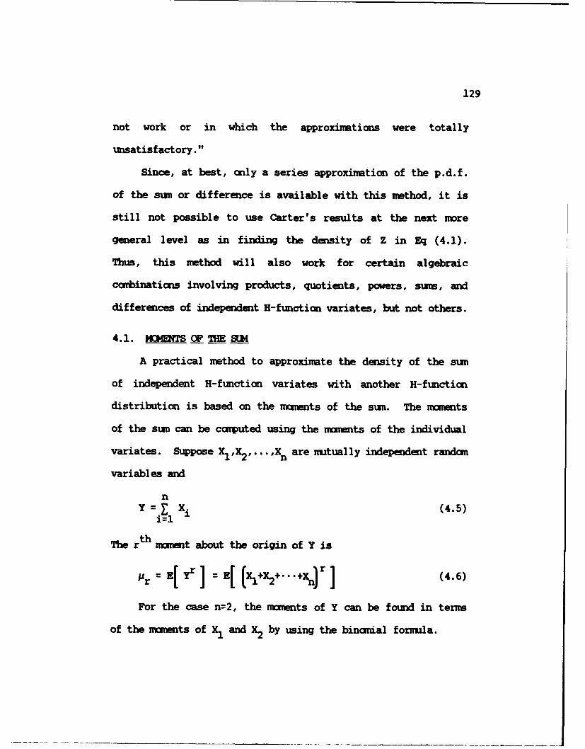
129

not work or in which the approximations were totally

unsatisfactory."

Since, at best, only a series approximation of the p.d.f.

of the sum or difference is available with this mthod, it is

still not possible to use Carter's results at the next more

general level as in finding the density of Z in Eq (4.1).

Thus, this method will also work for certain algebraic

combinaticns involving products, quotients, powers, sum, and

differences of independent H-fumction variates, but not others.

4.1. M3 DTS OF THE S34

A practical method to approximate the density of the sum

of independent H-function variates with another H-function

distribution is based on the moments of the sum. The mnents

of the sum can be coMputed using the mments of the individual

variates. Suppose X1,X2 ,... ,Xn are mutually independent randm

variables and

Y=- X1 (4.5)i=1

The rth moment about the origin of Y is

" [ ] -" FPr =E[# _E[(Xl+X2+...+Xr] (4.6)

For the case n-2, the maients of Y can be found in terns

of the moments of X1 and X2 by using the bincmial formula.

130

[r]r ~ (1) Y E[ X lri X21] (47

=r E [ r i X i ]

since matheratical expectation is a linear operator and and

X2 are independent. Here, is the bincmial coefficient

defined as

i = (4.8)i! (r-i)!

Eq (4.7) gives the maients of Y in terms of the moments of X,

and X2. There are r+1 term in the sum in Eq (4.7).

For the case rm2, the moments of Y can be found in terms

of the moments of X, to Xn by using a generalization of the

bincmial formfla.

pr]= E i'E[ 2-i+,2+..+Xnxr"

=EZ i1 i2! in! X I 2 ii

131

r! E[ [ 1 x2 . n

r!i!21"'" in! " [ ] (49)

where the sun is over all il,i 2,.... i n such that

ni= = r (4.10)j1 3

Here, the multinamial coefficient replaces the binomial

coefficient. Eq (4.9) gives the mauents of Y in terns of the

mcments of X1 through Xn . There are ( r+n1 ) terms in the sum

in Eq (4.9).

4.2. H-PUNCTION PARAMETR ESTIMATES

It is possible to use the moments of an H-function to

estimate its parameters. Bodenschatz and Boedigheimer [1983;

Boedigheimer et al, 1984] developed and verified an effective

and reliable method to estimate the H-function parameters using

the method of moments. The technique can be used to curve-fit

a mathematical function or to estimate the density of a

particular probability distribution. Their PFTRM computer

program will accept known monents, univariate data, ordered

132

pair data from a relative frequency, or ordered pair data

directly from the function. Output from the program are the

parameters of the H-function whose nmoents mst closely notch

the given maments.

This technique to estimate the parameters of the H-

function from the exact mments of an unknown distribution was

also generally described by Jacobs et al [1987]. A more

complete derivation is given below, which also shows how,

through algebraic nnipulation, it is possible to reduce the

nurber of equations by two.

4.2.1. METHOD OF MCM4ETS

The method of nments equates an appropriate number of

analytic nmnts of the H-function with corresponding known

nments or nmmnts calculated from data. The method uses

2(p+q)+2 nanmnts because there are this nany parameters in an

H-function distribution. This produces a system of nonlinear

equations in the parameters of the H-function.

Eq (4.9) gives the exact moments of a sum of independent

variates in terms of the moments of the individual variates.

If each random variable in the sum follows an H-function

distribution, the exact moments of the individual variates are

available by Eq (3.5). Using these moments in Eq (4.9) yields

the exact moments of the sum of independent H-function

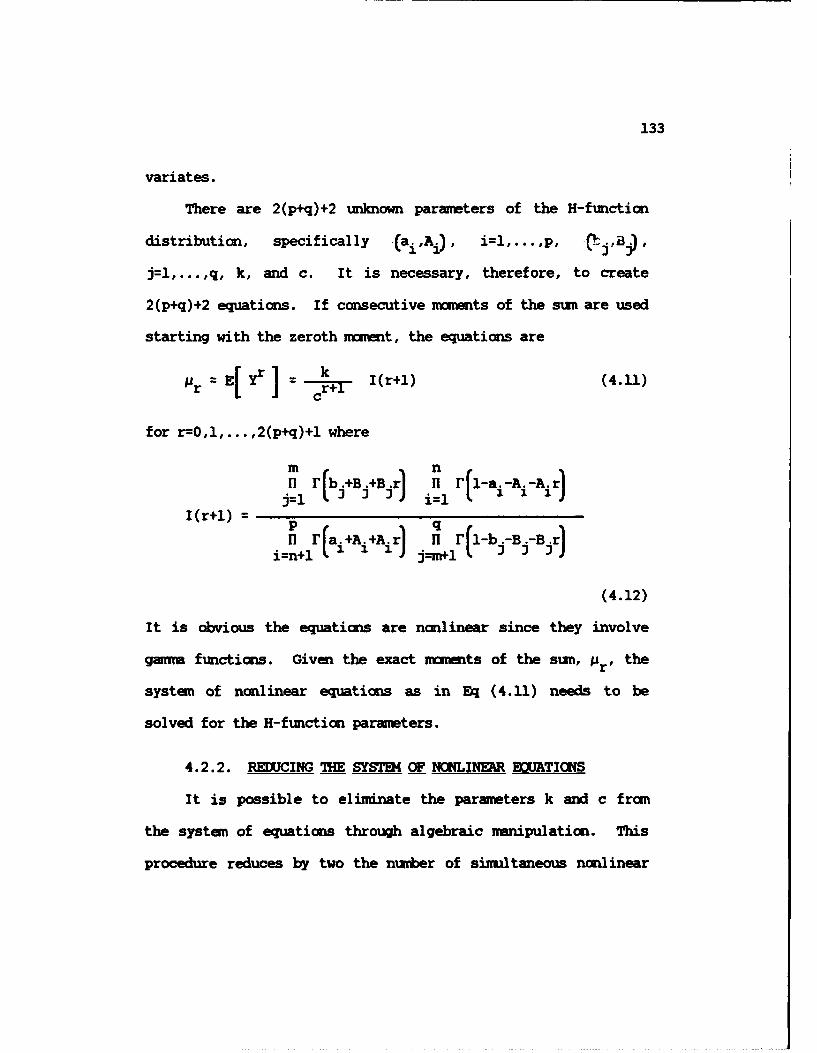
133

variates.

There are 2(p+q)+2 unknown parameters of the H-function

distribution, specifically (ai,Ai), i0,...,p, !jPB ) I

j=l,...,q, k, and c. It is necessary, therefore, to create

2(p+q)+2 equations. If consecutive moments of the sum are used

starting with the zeroth moment, the equations are

Mr = E[ yr k I(r+l) (4.11)c

for r=0,1,... ,2(p+q)+l where

m nn r (b +B +Bjr n r(1-ai-A. -A.r)j=l _+B_+B_ i= 1i1

I(r+1) =

n Fa.+A. +A. r)l n r(1-b.-B.-B.r)i~n+l Jj--M+l JJ

(4.12)

It is obvious the equations are nonlinear since they involve

gagin functions. Given the exact zoments of the sum, pr' the

system of nonlinear equations as in Eq (4.11) needs to be

solved for the H-function parmeters.

4.2.2. REXJCING THE SYSTE4 OF NChLINEAR E=TINS

It is possible to eliminate the parameters k and c from

the system of equations through algebraic manipulation. This

procedure reduces by two the number of simultaneous nonlinear

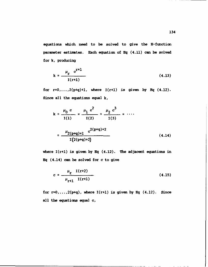
134

equatims which need to be solved to give the H-fumction

parameter estinates. Each equation of Eq (4.11) can be solved

for k, producing

r+1

k = (4.13)I(rl)

for r=0,...,2(p+q)+l, where I(r+1) is given by Fq (4.12).

Since all the equations equal k,

2 3k 0 c Ill c = 2 c

1(1) 1(2) 1(3)

P2(p)+I 2 (P+q)+22 M (pq) +, c (4.14)

I.(2(p+q)+2)

where I(r+l) is given by Eq (4.12). The adjacent equations in

Eq (4.14) can be solved for c to give

Pr I(r+2) (4.15)

Ir+1 I(r+1)

for r=O,... ,2(p+q), where I(r+1) is given by Eq (4.12). Since

all the equations equal c,

135

PO 1(2) p 1 I(3)_ _ _ _ --- _ _

1 1(1) 'J (2)

P2(p+q) I(2(p+q)+2) (4.16)

P2(p+q)+l I.C2(P+q)+l)

where I(r+l) is given by Eq (4.12). The adjacent equations in

Eq (4.16) can be solved to give the following homgeneous

equations:

Pi Pi+2 (I(i+2))2 1 = (4.17)"(Pi+1)2 I(i+l) I(i+3)

for i=O,...,2(p+q)-l, where I(r+1) is given by Eq (4.12). This

reduced system of equations involves only the H-function

parameters (ai,A1 ), i=l,...,P, and pj,B. , j1l,...,q.

once the nonlinear system of equations in Eq (4.17) is

solved, c and k can be found by backsubstitution. Using

Eq (4.16),

P0 1(2) (4.18)

p1 1(1)

where I(r+1) is given by Eq (4.12). Using this estimate of c

in Eq (4.14) produces

136

k P0 (4.19)1(1)

where I(r+1) is given by Eq (4.12).

Note that although this algebraic manipulation has reduced

the number of equations from 2(p+q)+2 to 2(p+q), all 2(p+q)+2

monments of the sum are still necessary.

4.2.3. SOLVING THE SYSTEK OF NONLINERR EDATICIS

Even after reducing the system of nonlinear equations by

two, there will always be at least two simultaneous equations

involving gamma functions. To complicate matters further, the

unknowns (the H-function parameters) appear in the argument of

every gamma function. A general analytic solution seems

unlikely, if not impossible.

Bodenschatz and Boedigheimer [1983] conducted a literature

review of various numerical methods applicable to the problem.

Most methods are based on Newton's method, which uses the

Jacobian matrix of first partial derivatives to move toward the

solution.

Powell developed a quasi-Newton hybrid algorithm which

includes the beneficial features of the Levenberg-Marquardt

method and implements the calculation-saving strategy of

Broyden's procedure. Powell's method was available in an

137

International Mathematical and Statistical Library (IMSL)

routine named ZSPOC. In comparison to available software

designed to solve system of nonlinear equations, ZSPOW had

outstanding performance and initial estimates of the parameters

had little effect on the algorithm's super linear convergence

[Hiebert, 1980].

Bodenschatz and Boedigheimer [1983] used ZSPOW to solve

many system of nonlinear equations as in Eq (4.17) with great

success. In their FORTRAN computer program, they allow the

user to make initial estimates of the H-function parameters and

also provide default guesses which nearly always led to

convergence to the correct parameters.

When trying to fit a third- or higher-order H-function,

however, the numerical solution of the system of nonlinear

equations with ZSPCW is sometimes numerically unstable.

Several other numerical methods were tried, but none worked as

well as ZSPOW in solving the type of nonlinear equations

generated using the method of oments with the H-function. An

area of further research is to develop a better way to solve

the system of nonlinear equations.

Jacobs et al [1987] discussed using equations as in

Eq (4.11) to estimate the parameters of an H-function if the

exact monits, M r' of the unknown distribution were available.

138

They also gave analytic solutions to these equations for

certain first order H-function distributions with B=1 or1

B= .However, restrictions such as these nay not give an H-

function with as good a fit to the mnents as an unrestricted

solution to the equations might allow.

* 4.3. SPECIAL CONSIDERATIONS FOR TYPE VI H-FUNCTION VARIATES

Sums of certain H-function distributions have special

properties which allow an analytic solution to the system of

nnonlinear equations. For example, if Y = i where the X.il=1 1

are mutually independent random variables which have beta

distributions over (0,I), then the p.d.f. of Y will be nonzero

nonly over (O,n). Similarly, if Y = X. where the Xi are

mutual ly independent random variables which have Pareto

distributions over (1,a)), then the p.d.f. of Y will be nonzero

only over (n,w). A new way to take advantage of these ranges

was discovered which eliminates the need for a numerical

solution to the system of nonlinear equations.

Certain simplifications occur if each H-function

distribution in the sum is a Type VI convergent H-function

according to Table 1 in Section 2.3. Because the sum

described above will also have restricted ranges, they must

also be Type VI convergent H-functions. Sections 2.6 and 3.6

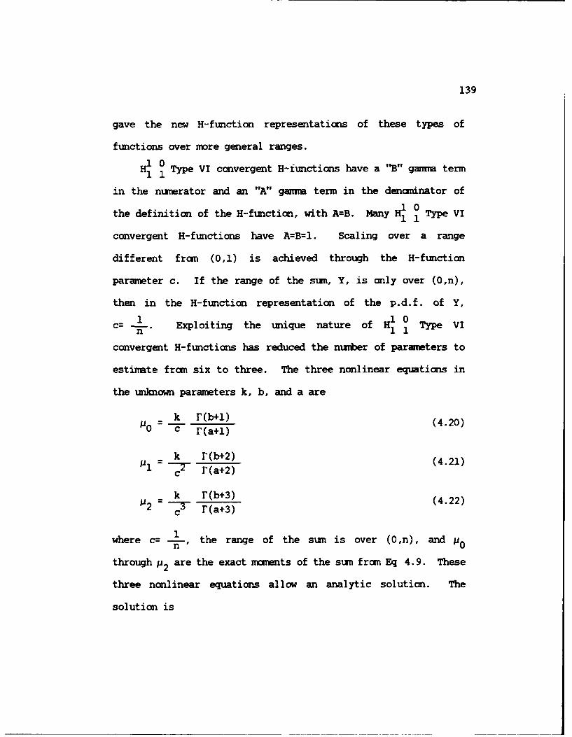
139

gave the new H-function representations of these types of

functions over more general ranges.

i0 Type VI convergent H-tunctions have a "B" gamma term11

in the numerator and an "A" gamma term in the dencminator of

the definition of the H-function, with A=B. Many H Type VI

convergent H-functions have A=B=I. Scaling over a range

different from (0,1) is achieved through the H-function

parameter c. If the range of the sum, Y, is only over (0,n),

then in the H-function representation of the p.d.f. of Y,

C= -. Exploiting the unique nature of H1 Type VIn 11convergent H-functions has reduced the number of parameters to

estinate frm six to three. The three nonlinear equations in

the unknown parameters k, b, and a are

k r(b+1) (4.20)0 c r(a+1)

= k r(b+2) (4.21)I = 7 r(a+2)

k r(b+3) (4.22)= r (a+3)

where c= -- , the range of the sum is over (O,n), and pO

through P2 are the exact mnamnts of the sum frm Eq 4.9. These

three nonlinear equations allow an analytic solution. The

solution is

140

P O Pl 'JO '2

a- - (P-) POP2 - (P.1)

(4.23)

b = c- P (a+1) - 1 (4.24)

k = poc r(a+1) (4.25)r(b+l)

where c and p0 through P2 are as given above. A possible H-

function representation for the density of the sum of H 01 1

VI convergent H-functions is

* f(y) = k H -Lny : (a,i) ; (b,l) (4.26)

where the range of the sum is over (0,n) and a, b, and k are

given by Eq (4.23), Eq (4.24), and Eq (4.25), respectively.

A similar approach applies to sums of H0 1 Type VI1 1 Tp

convergent H-functions which have an "A" gamma term in the

numerator and a "B" gama term in the denominator of the

definition of the H-function, with A=B. Again, let A:B=l.

Scaling over a range different fron (1,w) is achieved through

the H-function parameter c. If the range of the sum, Y, is

over (n,w), then in the H-function representation of the p.d.f.

of Y, C= 1 . Exploiting the unique nature of H 1 Type VI

convergent H-functions, the three nonlinear equations in the

141

unknown parameters k, b, and a are

k (-a) (4.27)0- c r(-h)

k r(-a-1) (4.28)1 - r(-b-1)

P k r(-a-2) (4.29)c - (-b-2)

1where c= -- , the range of the sum is over (n,), and p0

through P2 are the exact moments of the sum from Eq 4.9. These

three nonlinear equations again allow an analytic solution.

The solution for the unknown parameters a, b, and k is

identical to the ones given by Eq (4.23), Eq (4.24), and

Eq (4.25), respectively. A possible H-function representation

f or the density of the sum of H1 Type VI convergent H-1 1 Tp

functions is

* f(y) = k H [ --- y : (a,l) ; (b,l) (4.30)

where the range of the sum is over (ns) and a, b, and k are

given by Eq (4.23), Eq (4.24), and Eq (4.25), respectively.

* 4.4. DEDNSTRATI0N OF THE TECHNIGME

A FORTRAN computer program was developed to implement the

new technique of finding an H-function distribution which

approximates the distribution of the sum of two or more

142

independent H-function variates. The cauputer program was

designed to run interactively, asking questions of the user and

expecting a response.

Input to the program can be done interactively or through

an input file. A user will input the number of terms

(independent randm variables) in the sum and the type of each

variate. As currently configured, the program will accept up

to five terms in the sum. The type of each variate my be one

of the named special cases or a general H-function

distribution. If the type is a special case, the program will

convert the parameters of the special case into the correct H-

function parameters for the H-function representation.

Alternatively, a user my input the H-function parameters

directly.

The program will then ccmpute, using Eq (3.5), the correct

mnts of each H-function variate in the sum. The program

will verify a zeroth moment of unity and query the user if the

H-function parameters do not give a valid density. If desired,

the program will recompute the constant k to produce a valid H-

function distribution. The nanents of each term in the sum are

used as in Eq (4.9) to compute the exact murents of the sum.

If the sum involves only 0 Type VI H-function1 1distributions orcH0 1

0 1 Type VI H-function distributions, thedistibuionsor 1 1

143

analytic solutions for the H-function parameters derived in

Section 4.3 are used. Otherwise, an adapted version of the

program of Bodenschatz and Boedigheimer [1983] is called to

create and solve, using ZSPOW, the system of nonlinear

equations as in Eq (4.17). This produces parameters of the H-

function distribution whose moments will closely match the

exact moments of the sum.

If there are only two term in the sum, an atteffpt can be

made to fit an H-function distribution with up to five gamma

term (fifth-order). If there are more than two terms in the

sum, the program currently computes only the zeroth through the

fifth momnts about the origin of the sum. This limits the

choice of an H-function distribution for the sum to a first- or

second-order H-function.

This is not a serious restriction for two reasons. First-

and second-order H-function distributions can represent a wide

variety of distributional forms, including nearly every named

special case. Secondly, numerical and computational

limitations exist in finding the moments of the sum and solving

large systems of nonlinear equations with ZSPOW. Until these

limitations are addressed, an attempt to fit a third- or

higher-order H-function would probably not be successful.

The moments of the new H-function distribution are

144

computed for comparison to the exact noments of the sum. The

program will then, if desired, create an input file for another

cumputer program [Cook, 1981; Cook and Barnes, 1981] which will

evaluate and plot the resulting p.d.f. and c.d.f.

An output file is always created, giving the H-function

parameters and moments of each term in the sum, the exact

moments of the sum, the estimated H-function parameters, and

the moments of this new H-function distribution.

The FORTRAN source code of the cumputer program described

above is not provided in an appendix. Instead, it is available

fram Dr. J. Wesley Barnes in the Department of Mechanical

Engineering at the University of Texas at Austin. If

requested, Dr. Barnes will transfer the program by electronic

mail or by floppy disk.

The new FORTRAN coaputer program which inplements the

technique currently operates on the instructional VAX cluster

at the University of Texas at Austin. This cluster links two

VAX 6420 ccvputers and several VAX 11/780 computers and uses

the VMS operating systen. The VAX FORTRAN compiler was used

and the program linked to IMSL for the call to ZSPOW. The

program should successfully run on other cc2Puters which

support ZSPOW in IMSL and which have ANSI FORTRAN capabilities.

The new technique and computer program are demonstrated in

145

the following examples. In all but the final example, it is

possible to find the exact distribution of these sums of

variates by other methods. Thus, we can easure the

effectiveness of the new technique by comparing the resulting

H-function distribution to the exact distribution. Of course,

the new technique also works with sums for which the solution

by other methods is very difficult (or impossible for all

practical purposes).

4.4.1. EXAMPLE 1 - SUM OF THREE INDEPENDENT, IDENTICALLY

DISTRIBUTED GAM4A VARIATES

Suppose we want to use this technique to find the H-

function distribution of the sum of three independent,

identically distributed ganria variates with parameters r=2 and

X=2. Using the computer program, we input "3" as the number of

terns in the sum, "gamma" as the type of each variate, and the

parameters "2" for r and "2" for X.

The moments of each variate in the sum are computed and

combined to give the exact monents of the sum. These are

M0 = 1.0000000 Pi = 3.0000000

I2 = 10.5000000 P3 = 42.0000000

P4 = 189.0000000 P5 = 945.0000000

The program asks whether we want to fit an H-function

distribution to the mments of the sum and, if so, the order of

146

H-function to fit. Since all three variates in the sun are

first order H-functions, we try to fit another first order H-

function. We enter "1 0 0 1" for m, n, p, and q, respectively.

The program uses the zeroth through third moments of the sun to

create and solve the system of nonlinear equations, producing

the H-function parameter estimates

b = 4.99999988853

B = 0.99999999256

k = 0.01666666667

c = 2.00000000000

Allowing for roundoff error, we recognize these as the

parameters of the H-function representation of the gamma

distribution with r=6 and X=2. The procedure found the

"correct" distribution since the gamma distribution with a

counon X has the reproductive property. The program

automatically uses these H-function parameters to compute the

moiments of the new H-function distribution.

P0 = 1 0000000 Pi = 3.0000000

P2 = 10.5000000 P3 = 42.0000000

P4 = 189.0000000 p5 = 945.0000000

The program then asks whether we want to create an input

file for another conputer program [Cook, 1981; Cook and Barnes,

1981] which will evaluate and plot the resulting p.d.f. and

147

c.d.f. If so, it asks the range and interval of the variable

where we want these functions evaluated. We try the range 0.1

to 7.0 with an interval of 0.1. The complete output file is

provided in Appendix A.

4.4.2. EXAMPLE 2 - SUM OF IWO INDEPENDENT ERLANG VARIATES

WITH DIFFNT X

Suppose we want to find an H-function distribution for

Y = XI+X2 where X1 has an Erlang (gamma) distribution with

parameters r=2 and X=4 and X2 has an Erlang (gamma)

distribution with parameters r=1 and X=2. Note that X2 also

has an exponential distribution with X=2. Using the computer

program, we input "2" as the number of terms in the sum,

"gamma" as the type of each variate, the parameters r="2" and

X="4" for XI , and the parameters r="l" and X="2" for X2 . Of

course, we could have input X2 as type "exponential" with )="2"

or input both random variables as general (unnamed) H-function

variates by giving their H-function parameter representations.

The moments of each variate in the sum are ccmputed and

combined to give the exact moments of the sun. These are

10 = 1.0000000 I = 1.0000000

P2 = 1.3750000 g3 = 2.4375000

P4 = 5.3437500 P5 = 14.0625000

P6 = 43.4179688 P7 = 154.4238281

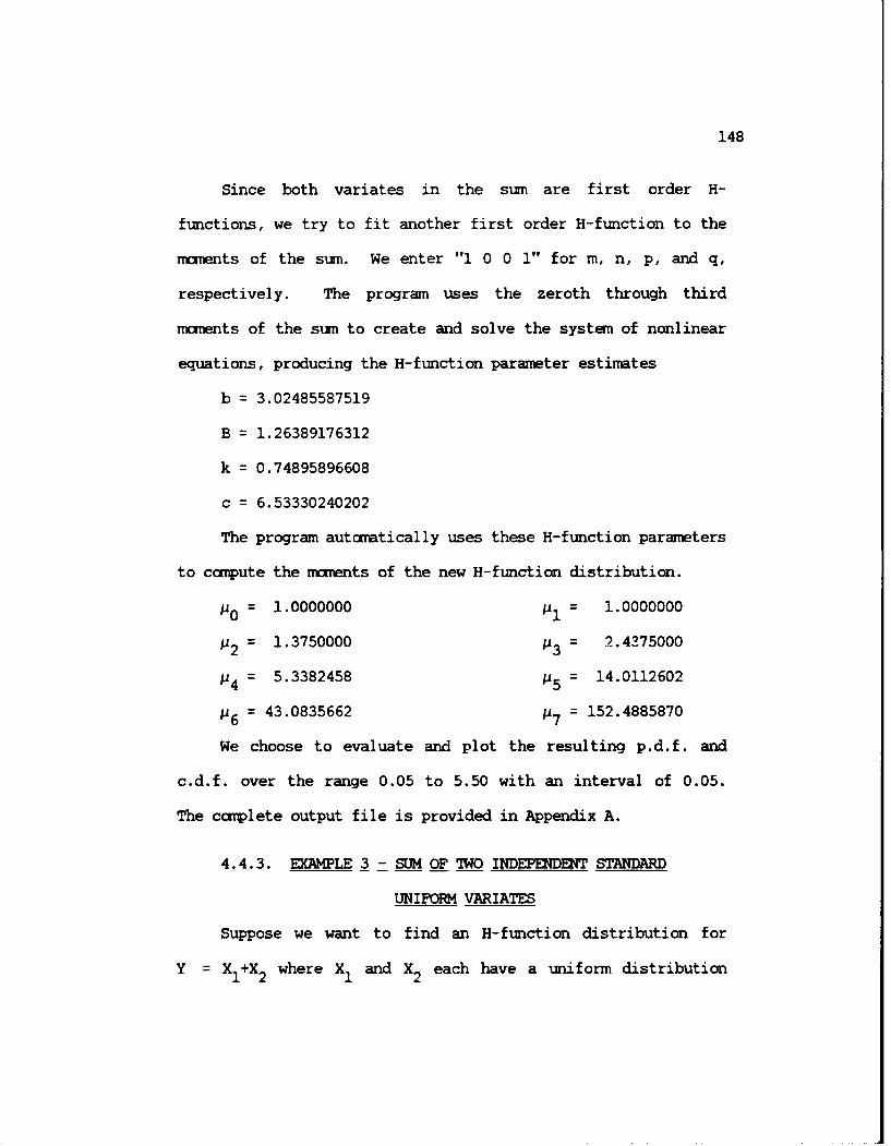
148

Since both variates in the suxn are first order H-

functions, we try to fit another first order H-function to the

moments of the sun. We enter "1 0 0 1" for m, n, p, and q,

respectively. The program uses the zeroth through third

monents of the sun to create and solve the system of nonlinear

equations, producing the H-function parameter estimates

b = 3.02485587519

B = 1.26389176312

k = 0.74895896608

c = 6.53330240202

The program automatically uses these H-function parameters

to compute the maments of the new H-function distribution.

P0 = 1.0000000 Pi = 1.0000000

P2 = 1.3750000 U3 = 2.4375000

P4 = 5.3382458 P5 = 14.0112602

P6 = 43.0835662 IJ7 = 152.4885870

We choose to evaluate and plot the resulting p.d.f. and

c.d.f. over the range 0.05 to 5.50 with an interval of 0.05.

The complete output file is provided in Appendix A.

4.4.3. EXAMPLE 3 - SUM OF 7WO INDEPENDEN4T STANDARD

UNIFORM VARIATES

Suppose we want to find an H-function distribution for

Y = XI+X2 where X1 and X2 each have a uniform distribution

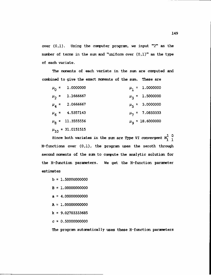
149

over (0,1). Using the computer program, we input "2" as the

nuznber of terms in the sun and "uniform over (0,1)" as the type

of each variate.

The mnents of each variate in the sum are computed and

combined to give the exact moments of the sun. These are

P0 = 1.0000000 Pi = 1.0000000

P2 = 1.1666667 P3 = 1.5000000

114 = 2.0666667 P5 = 3.0000000

P6 = 4.5357143 17 = 7.0833333

P8 = 11.3555556 p9 = 18.6000000

Pi0 = 31.0151515

Since both variates in the sun are Type VI convergent Hi 10

H-functions over (0,1), the program uses the zeroth through

second moments of the sum to compute the analytic solution for

the H-function parameters. We get the H-function parameter

estimates

b = 1.50000000000

B = 1.00000000000

a = 4.00000000000

A = 1.00000000000

k = 9.02703333685

c = 0.50000000000

The program automatically uses these H-function parameters

150

to compute the moments of the new H-function distribution.

110 = 1.0000000 i = 1.0000000

;J2 = 1.1666667 P3 = 1.5000000

P 4 = 2.0625000 P5 = 2.9791667

M6 = 4.4687500 P7 = 6.9062500

P8 = 10.9348958 P9 = 17.6640625

Pio = 29.0195312

We choose to evaluate and plot the resulting p.d.f. and

c.d.f. over the range 0.05 to 2.00 with an interval of 0.05.

The corplete output file is provided in Appendix A.

4.4.4. EXAMPLE 4 - SUM OF TWO INDEPENDENT, IDENTICALLY

DISTRIBUTED BETA VARIATES

Suppose we want to find an H-function distribution for

Y = XI+X2 where X1 and X2 are independent variates with beta

distributions over (0,1) with parameters a=l and P=2. Using

the ccrputer program, we input "2" as the number of term in

the sum, "beta over (0,1)" as the type of each variate, "1" for

a, and "2" for P.

The moients of each variate in the sum are computed and

combined to give the exact nuxents of the sun. These are

P0 = 1.0000000 Mi = 0.6666667

P2 = 0.5555556 P3 = 0.5333333

P4 = 0.5666667 P5 = 0.6507937

151

P6 = 0.7952381 17 = 1.0222222

P8 = 1.3703704 19 = 1.9030303

10 = 2.7229437

Since both variates in the sum are Type VI convergent H1 011

H-functions over (0,1), the program uses the zeroth through

second muments of the sun to coMpute the analytic solution for

the H-function parameters. We get the H-function parameter

estimates

b = 1.33333333333

B = 1.00000000000

a = 6.00000000000

A = 1.00000000000

k = 302.35856086513

c = 0.50000000000

The program automatically uses these H-function parameters

to compute the moments of the new H-function distribution.

P0 = 1.0000000 1 = 0.6666667

P2 = 0.5555556 P3 = 0.5349794

14 = 0.5706447 P5 = 0.6571060

116 = 0.8031296 17 = 1.0296533

M8 = 1.3728711 19 = 1.8915113

110 = 2.6796410

We choose to evaluate and plot the resulting p.d.f. and

152

c.d.f. over the range 0.05 to 2.00 with an interval of 0.05.

The complete output file is provided in Appendix A.

4.4.5. EXAMPLE 5 - SUM OF TWO INDEPEN4DE4T VARIATES WITH

WEIBULL AND RAYLEIGH DISTRIBUTIONS

A final example demonstrates the technique and computer

program when the exact distribution of the sum is very

difficult or impossible to obtain.

Suppose we want to find an H-function distribution for

Y = XI+X2 where X1 has a Weibull distribution with parameters

P=5 and X=4 and X2 has a Rayleigh distribution with parameter

X=3. Using the computer program, we input "2" as the number of

terms in the sum, "Weibull" as the type of variate X1 with

parameters 0="5" and X="4", and "Rayleigh" as the type of

variate X2 with parameter X="Y'. Of course, we could have

input both random variables as general H-function variates by

giving their H-function parameter representations.

The mmnts of each variate in the sum are computed and

combined to give the exact mients of the sum. These are

M0 = 1.0000000 P1 = 1.2075051

112 = 1.5550061 93 = 2.1228284

P 4 = 3.0567312 P5 = 4.6225066

P6 = 7.3134235 P7 = 12.0647384

P8 = 20.6900000 P9 = 36.7858797

153

00 = 67.6453356

Since both variates in the sum are first order H-

functicns, we try to fit another first order H-function to the

moments of the sum. We enter "l 0 0 1" for m, n, p, and q,

respectively. The program uses the zeroth through third

moments of the sum to create and solve the system of nonlinear

equations, producing the H-function parameter estimates

b = 5.29104742893

B = 0.62358286635

k = 0.02369785777

c = 2.45993399245

The program automatically uses these H-function parameters

to compute the mrnents of the new H-function distribution.

10 = 1.0000000 i1 = 1.2075051

i2 = 1.5550061 p3 = 2.1228284

04 = 3.0568212 V5 = 4.6235079

;6 = 7.3191453 ;.7 = 12.0889706

08 = 20.7770136 p9 = 37.0686930

io = 68.5084603

We choose to evaluate and plot the resulting p.d.f. and

c.d.f. over the range 0.05 to 2.40 with an interval of 0.05.

The complete output file is provided in Appendix A.

CHAPTER 5

CCHPARING THE ESTIMATED H-FUNCTION TO THE

EXACT DISTRIBUTION OF THE SUN

It is natural to want to measure the effectiveness of the

newly developed technique which finds an H-function

distribution whose mments closely approximate the exact

moments of the sum of independent H-function variates.

Ideally, the approximate H-function distribution should be

compared to the exact distribution for the sun. Unfortunately,

the exact distribution of the sum is often difficult to obtain.

Because of this, analysts usually resort to computer simulation

to 9!ialyze the resulting distribution. Even this approach

yields only information about the resulting distribution, not

the exact density itself.

Four examples included in this thesis were chosen as

representative of sums of independent H-function variates where

the oxact distribution of the sum can be obtained. A FORTRAN

ccnpvter program was written to compare the approximate H-

function distribution to the exact distribution for the surn,

using several different measures of merit. The newly developed

154

155

technique was also effective in finding an H-function

distribution whose moments closely approximate the exact

rments of the sun even when the exact distribution is very

difficult or in-possible to obtain.

5.1. FINDING THE EXACT DISTRIBUTION OF THE SUM

As mentioned above, it is often difficult to obtain the

exact distribution for the sun of independent random variables.

While the moment generating function, Laplace transform, or

characteristic function (Fourier transform) of specific

densities are sometimes available from tables, the product of

these transform functions will often produce a functional form

that is not easily inverted.

Suppose XlX 2,... X n are mutually independent randon

variables with respective densities f1 (xl), f 2 (x) ...

fn(x,)i each nonzero only for positive values of the variable.

nSuppose we want the density of Y = X.. If the Laplacei=1

transforms of the densities are Zs{fl(x1 )}, rs{f 2 (x 2)1'

Sn respectively, then the density of Y is available as

the inversion integral

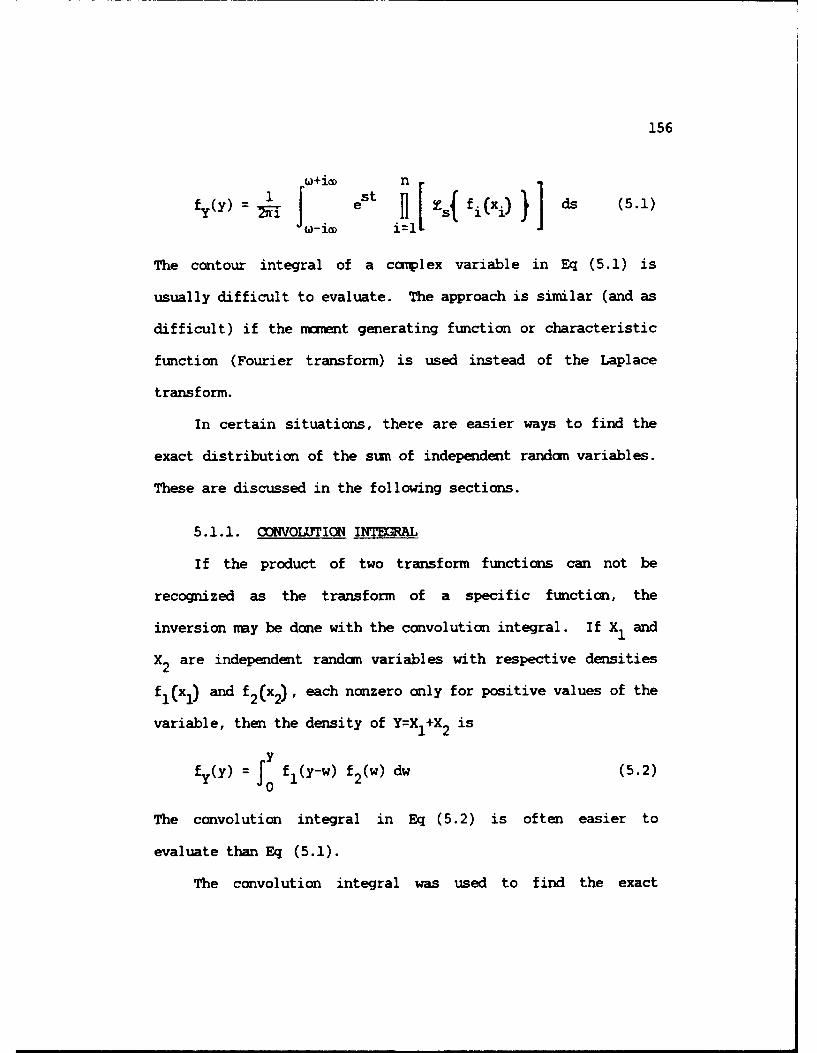
156

u+icD nfyy - e H Z s 1 f i (xi) ds (5.1)

-iO i=11

The contour integral of a complex variable in Eq (5.1) is

usually difficult to evaluate. The approach is similar (and as

difficult) if the moment generating function or characteristic

function (Fourier transform) is used instead of the Laplace

transform.

In certain situations, there are easier ways to find the

exact distribution of the sum of independent random variables.

These are discussed in the following sections.

5.1.1. CONVOLUTIM4 INTEGRAL

If the product of two transform functions can not be

recognized as the transform of a specific function, the

inversion may be done with the convolution integral. If X1 and

X2 are independent random variables with respective densities

fI(Xl) and f 2 (x2), each nonzero only for positive values of the

variable, then the density of Y=XI+X2 is

f (y) = f f(Y-w) f2 (w) dw (5.2)

The convolution integral in Eq (5.2) is often easier to

evaluate than Eq (5.1).

The convolution integral was used to find the exact

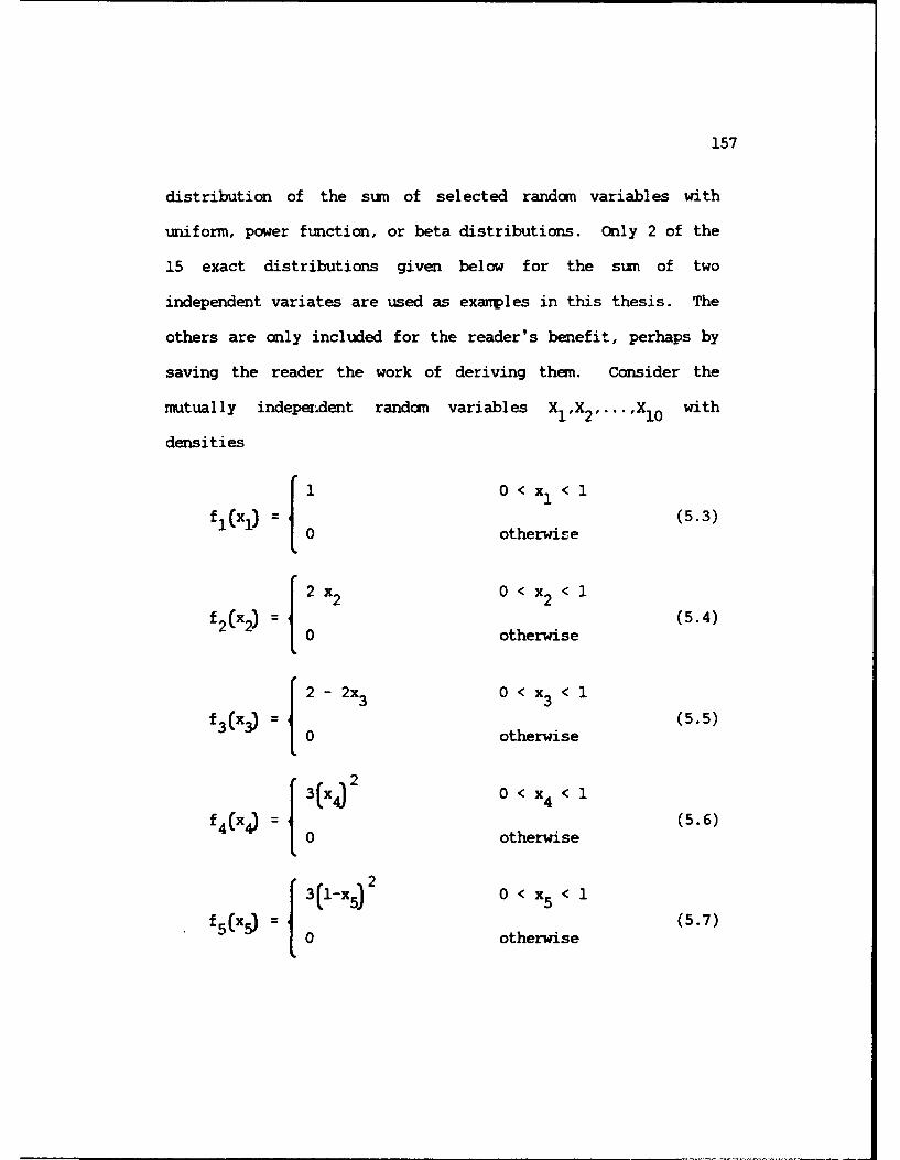
157

distribution of the sum of selected random variables with

uniform, power function, or beta distributions. Only 2 of the

15 exact distributions given below for the sum of two

independent variates are used as examples in this thesis. The

others are only included for the reader's benefit, perhaps by

saving the reader the work of deriving them. Consider the

mutual ly indeperdent random variables X1 ,x 2 , ... ,XI0 with

densities

x = 0 otherwise (53)

2 x2 0 < x2 < 1

f2(x2)= 0 otherwise (5.4)

2 - 2x3 0 < x3 < 1

f3 (x 0 otherwise (5.5)

f'4N = 0 otherwise (5.6)

f (x (ote0 wis (5.6 )f 5(x = 0 otherwise(57

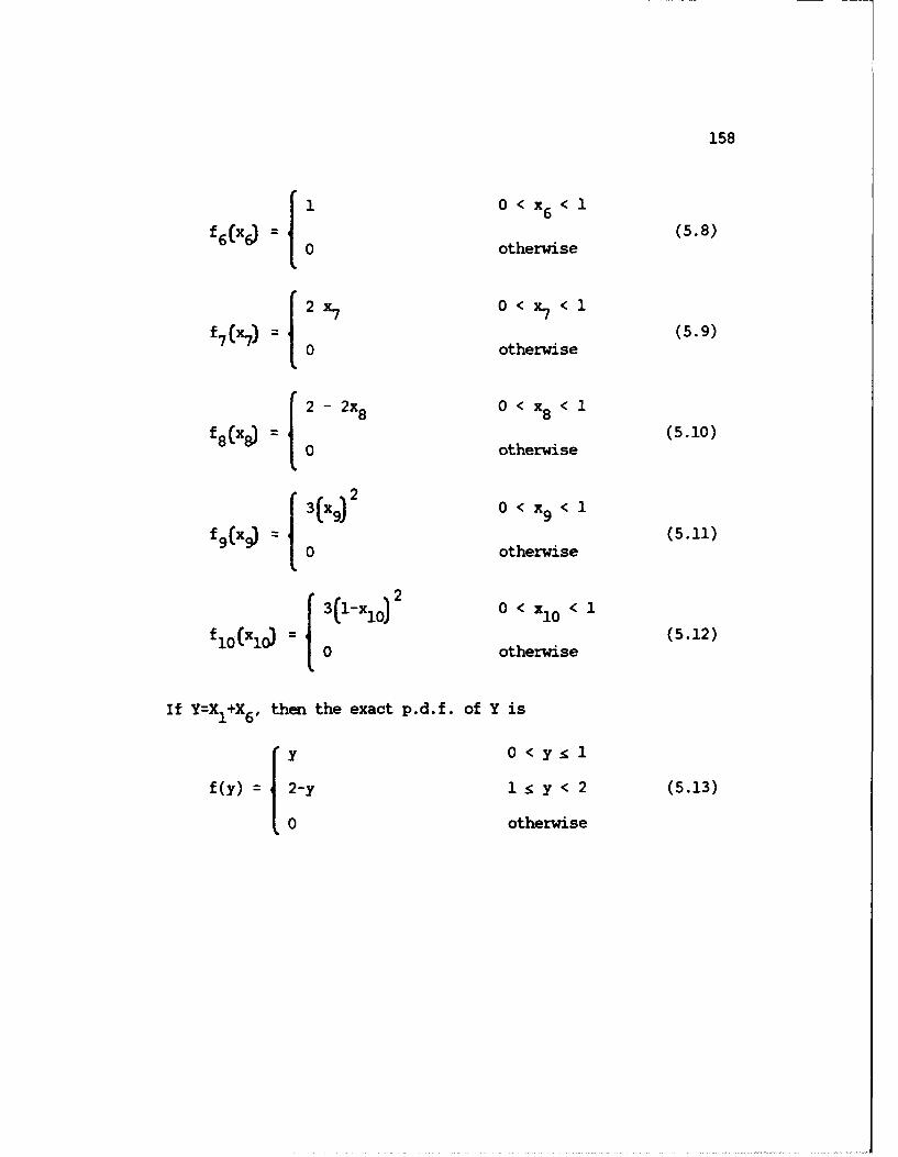
158

0 O<x6 <1

f 6 (xd = 0 otherwise (5.8)

r2 x 0 < x< 1f 7 (x7 ) = 0 otherwise (5.9)

2 - 2x 8 0 < x 8 < I

f18(x 0 otherwise (5.10)

f8( 8 (5.10)

f lOtxlo) 0 otherwise (5.12)

If Y=XI+X6, then the exact p.d.f, of Y isy O<xy I

f ( y) =2-y 1 y < 2 (5.13)

0 otherwise

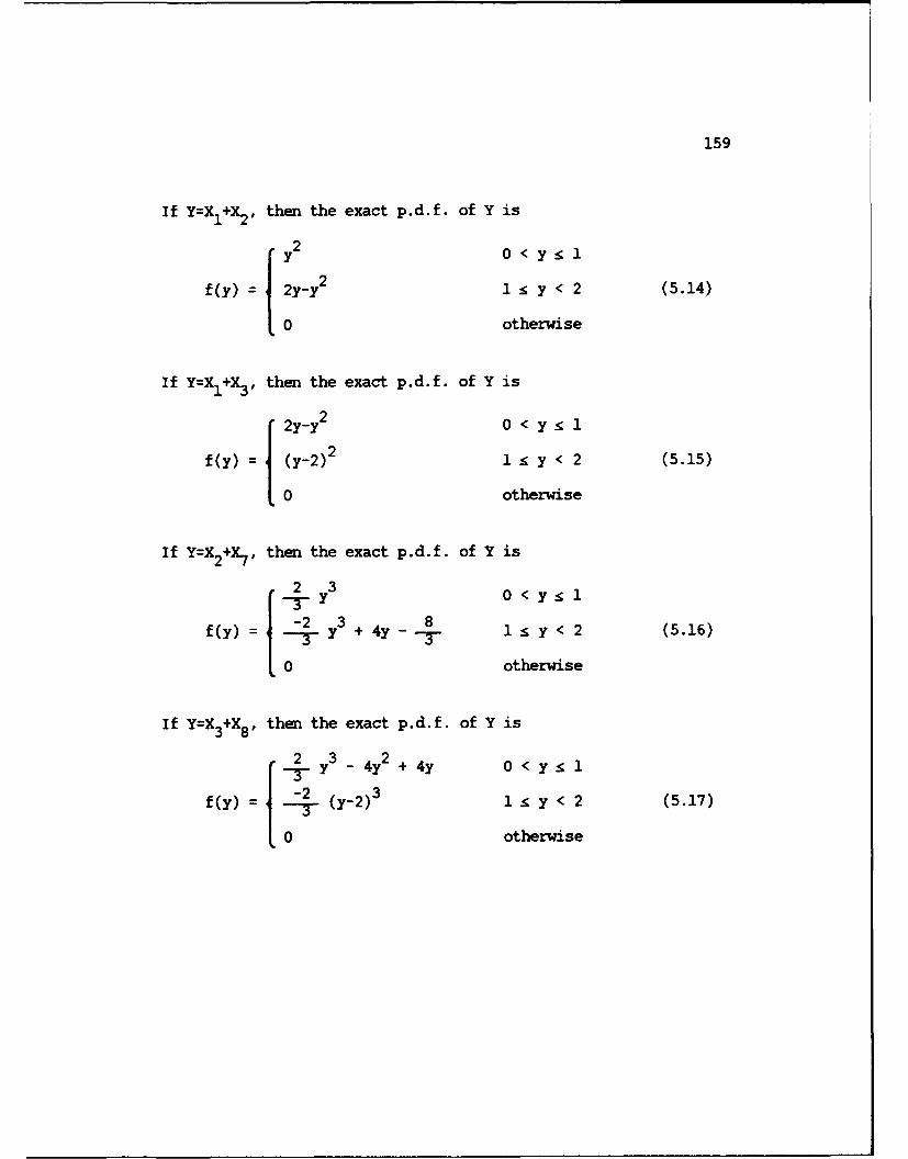
159

If Y=X1+X2p then the exact p.d.f. of Y is

y2 O<y l

f(y) - 2y-y 2 1 s y < 2 (5.14)

0 otherwise

If Y=XI+X 3 , then the exact p.d.f. of Y is

2y-y2 0 < y 1

f(y) = (y-2)2 1 s y < 2 (5.15)

0 otherwise

If Y=X2+X , then the exact p.d.f. of Y is

I 2 38

f(y) = - y3 + 4y - 8 1 - y < 2 (5.16)

0 otherwise

If Y=X3+X8, then the exact p.d.f. of Y is

2 3 2-_T2y - 4y + 4y 0 < yS 1

f(y) = (y-2) 3 1 s y < 2 (5.17)

0 otherwise

160

If Y=X2 +X 3, then the exact p.d.f. of Y is

-2 3+ 20 y 1

1~) 2 3 2 87-y 2y + 1-5y<2(-8

0 otherwise

if Y=X I+X 4,, then the exact p.d.f. of Y is

f(y) 1 - (y-1) 3 1 -- y < 2 (5.19)

0 otherwise

If Y=X1 +X5, then the exact p.d.f. of Y is

f(y) = -(y-2) 3 14y < 2 (5.20)

0 otherwise

If Y=X2+X4 ' then the exact p.d.f. of Y is

1 4 <~

f~y 2Y y - l 4y < 2 (5.21)

0 otherwise

161

If Y-X2+X5 F then the exact p.d.f. of Y is

1y4 _ 2y3 + 3y2 0 < y _r 1

f(Y) ={ 1 -y 4 + 2y 3 - 8y + 8 1 r y < 2 (5.22)

o otherwise

If Y=X3+X4, then the exact p.d.f. of Y is

-1 4 3~ ~-,r y + 2y0<y 1

f(y) = 24 _ 2y3 + 3y2 4y + 4 y < 2 (5.23)

0 otherwise

If Y=X3+X5, then the exact p.d.f. of Y is

-1 4 3 2r y + 4y -9y + 6y 0 < y < 1

f(Y) 4 1 y < 2 (5.24)

0 otherwise

If Y=X4+X9, then the exact p.d.f. of Y is

3 5W y~ 0 < y - 1

f(Y) = y y5 + 6y2 _ 9y + 181 y < 2 (5.25)

0 otherwise

162

If Y=X5+XI0, then the exact p.d.f. of Y is

y 5 3y4 + 12y3 18y2 + 9y 0 < y 1

f(y) 3 (y-2) 5 1 - y < 2

0 otherwise

(5.26)

If Y=X4+X5 , then the exact p.d.f. of Y is

3 5 3 4 +3 O < y <1-y- 2.~.y+3

-3 5 3 4 3 2 48

0 otherwise

(5.27)

These exact distributions could be compared to the

corresponding approxim-ate H-function distributions. The exact

distribution in Eq (5.13) is compared to the approximate H-

function distribution in Section 5.3.3 below. The exact

distribution in Eq (5.17) is cumpared to the approxirate H-

function distribution in Section 5.3.4 below.

Appendix B contains graphical depictions of the 15 exact

distributions in Eq (5.13) through (5.27) above. The graph of

the p.d.f. of each random variable in the sum is followed by

the graph of the p.d.f. of the sum. Each series of three

graphs is referenced to the corresponding equation number.

163

5.1.2. REPRODUCTIVE DISTRIBUTIONS

As discussed in Section 1.4.1.3, certain distributions

have the reproductive property, which considerably sinplifies

finding the exact distribution of the sum of independent random

variables with distributions of these form. The gamma

distribution is an H-function distribution with the

reproductive property, provided X is common among all

distributions in the sum.

nSuppose we want the density of Y = X. where

i= 1

XIX 2 .... ' Xn are nutually independent gamma distributed random

variables with respective paraeters (rl,)), (r 2 ) )..

(rnX), and X is camon to all the distributions. It is well

known that Y also has a gamma distribution with parameters

nr = r. and X. Since the exponential distribution is ai=1

special case of the gamma distribution with r=1, the sum of n

independent, identically distributed exponential randn

variables has a gamma distribution with parameters r=n and X.

This result is also widely known.

The reproductive property of the gamma distribution was

used to find the exact distribution of the sum of three

independent, identically distributed gamma variates. This

164

exact distribution is con-pared to the approximate H-function

distribution in Section 5.3.1 below.

* 5.1.3. ERLANG DISTRIBUTIONS WITH DIFFERENT

Another new finding permits finding the exact distribution

of the sum of independent Erlang distributed random variables,

even when X is different. An Erlang distribution is siuply a

gamma distribution with an integer shape parameter r.

Suppose we want the density of Y=X1+X2 where X1 and X2 are

independent Erlang distributed random variables with respective

parameters (rlXl) and (r2 ,X2), with )1 ) 2. The Laplace

transform of the density of Y is the product of the Laplace

transforms of the Erlang densities.

,r 1 r 2 r_102) ( 1 ( s 2 (5.28)

We proceed by decomposing the final two terms by partial

fractions. The approach presented below is essentially the

same as that described by Kleinrock [1975] and is routinely

given in texts covering Laplace transform including Churchill

[1972], Widder [1941], Thorpson [1960], Smith [1966], Doetsch

[1971), Davies [1978], or LePage [1961]. Since r1 and r2 are

165

positive integers in the Erlang distribution, we have X1 and X2

as (possibly repeated) linear factors of the denoinator.

S r ) ( 1) 2 Ar 1 -1 r 2-1

i C=i s+X2)1

(5.29)

To solve for the constants Aj, we first rewrite Eq (5.29)

as

rI

(~ ''2 r A. 1 -

r2 B

+ r r r2-1i(5.(s+1)2) (5.30)

We can inmediately solve for A0 by setting s=-X in Eq (5.30).

Hence,1 (5.31)

Then by taking successive derivatives of Eq (5.30) with respect

to s and evaluating both sides at s=-X I , we have

A. 1 d 1= (5.32)

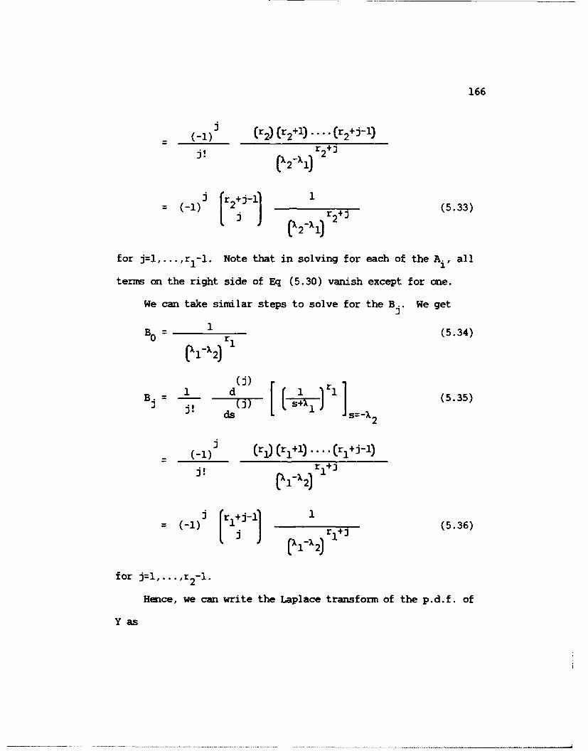
166

(-I) r2)( 2+) .... (r2+j-')

(-1) (r2 +l (5.33)

)4 2 -xi)

r2+

for j=l,.... 1rl1. Note that in solving for each of the Ai, all

terms on the right side of Eq (5.30) vanish except for one.

We can take similar steps to solve for the B. We get

11

B0 = Irl (5.34)

B. = 1 d [ - (5.35)ds

2

(-1) (ri) (r+l) .... (r 1 +j-1)

(-1) [rl+j-i] (5.36)r _ 1 +3

for j=l,...,r2-1.

Hence, we can write the Laplace transform of the p.d.f. of

Y as

167

r= r 2 r ]r, (.21) r 2 1r 2 (5.37)

(.)r I(2 r 2 1 Ar-i B r2-i= CLI) C 2 [ A i + Bs.2 1

=i S+Xl =i~

(5.38)

- r2+j-1)

= 1') (X'2) Er2 + 1 r,- j

r2 (-1 ) (ri+j -1

+ =0 h (-X2) r (s+X2)

(5.39)

We now use the linearity property of the inverse Laplace

transform to invert this transform term by term. We obtain the

p.d.f. of Y, fy(y).

168

*~~~ f-(y 3 ri 22_________

f 0- 1) 1(0-2)2r3=0 (b2"1) (rl-jrl)

r 1 -)- -Xyy e

r 2 1 (-)r 1 ] r - j-1 X2 y

+ ry 2 e 2

3=0 -X2 (r 2 -i-

(5.40)

*~-I - M 2

r 1-l (-1) [i2 r --____ ____ ____ ____ __

169

+ (x 1) ("1 02) r2eX2rI

y > 0

(5.41)

The result is sirply a sum of exponential and gamma-type term.

There are r1+r2 terms in the sum defining the p.d.f. of

YXI+X2 •

The practical rethod described above can be extended to

find the exact distribution of the sum of an arbitrary number

of independent Erlang randum variables. Suppose we want the

ndistribution of Y= Xi where X1 ..... n are independent Erlang

distributed random variables with parameters ri and Ii.

i=l,...,n. Also assume X. ) j for i~j. If any scale

parameters, X, were common among the random variables in the

sum, they could be immediately combined into another Erlang

random variable using the reproductive property.

We again decompose the product of Laplace transforms of

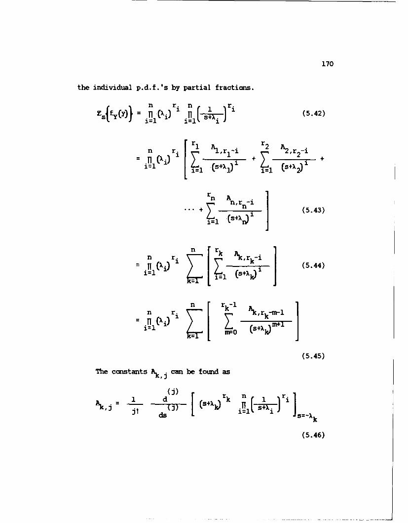
170

the individual p.d.f.'s by partial fractions.

n r. n f risjfyCy)) n r i n r (5.42)

11 A,rz-i + ,r~ 2-i1lX)i =1 (S+Xl)l I l = E sX) I

0 -,1=1 (s .4 2 )rn A

1=1 tS~xr)

n i) i n Aki (5.44)= i S+XW

nl r i r k- Ak'rk-m-i

i fi("i) i Z0 (s+Xk)m+

(5.45)

The constants Ak, j can be found as

(J1 d) [ rk n ri

5s 6k

(5.46)

171

for j=0,1, .... rk-i and k=1,2, ...,n.

We again use the linearity property of the inverse Laplace

transform to invert this transform term by term. We obtain the

np.d.f. of Y=.EXi, fy(y).

1

n r n rk-l y1

fy(y) An rIki) [ n- rke- JyO

y > 0

(5.47)

where Ak, j are as given in Eq (5.46) for j=0,1,... rk-i and

k=1,2, ...,n.

Eq (5.47) gives the exact p.d.f. for the sum of an

arbitrary number of independent Erlang random variables with

ndifferent scale parameters Xi . Note that there are E rk terns

k=1in the sum and each term has either an exponential or ganma-

type form.

This new result was used to find the exact distribution of

the sum of two independent Erlang variates. This exact

distribution is compared to the approximate H-function

distribution in Section 5.3.2 below.

172

5.2. MEASURES OF MEIT

There is no universally accepted measure to determine how

"close" an approximation is to the exact distribution. It is

likely that any standard statistical test for goodness of fit

(e.g. Chi-Square or Kolanogorov-Smirnov) would fail to reject

the null hypothesis that the approximate H-function

distribution and the exact distribution were equal. However,

this is because these tests are not very powerful or

discriminatory, not necessarily because the distributions are

nearly identical.

One way to compare the approximate H-function distribution

to the exact distribution involves comparing the corresponding

moments. Assuming ZSPcW successfully "solved" the system of

nonlinear equations, there should at least be a perfect Patch

of the moments used. For sums of variates where an analytic

solution for the H-function parameters was possible, at least

three nmments should match perfectly. Higher order moments of

the approximate H-function distribution may be in error to some

degree.

Although there is no standard measure of the "closeness"

of two distributions, there are several measures that are

commonly used. These are described below and computed for the

exanples listed. The measures were included in a FRTIRAN

173

ccmputer program which compares the approximate H-function

distribution to the exact distribution of the sum.

These measures, when considered collectively, give sate

idea of how well the approximate H-function distribution

matches the exact distribution of the sum of independent H-

function variates. Of course, the measures can only be

computed when it is possible to find the exact distribution of

the sum. In many cases, the exact distribution of the sum of

independent H-function variates is very difficult to obtain.

In the descriptions that follow, let the density of the

exact distribution of the sum of independent variates be

represented by f(y), let the density of the approximate H-

function distribution be H(y), and let each density be

evaluated at n equally spaced values of the variable. The

common interval between consecutive y values is Ay. The

densities should be evaluated over the whole range of values

the variable is likely to assume.

5.2.1. ESTIMATED SUMS OF SQUARES OF RROR

The estimated sums of squares of error (SSE) is obtained

by adding the squared difference between f(y) and H(y) for all

n values of the variable where the functions were evaluated.

174

n f2

5.2.2. ESTIMATED MEAN SQUAREDRROR

Unless f(y) and H(y) are identical, the estimated SSE will

increase if n is increased. This limitation of the estimated

SSE is corrected by dividing by n, yielding the estimted mean

squared error (MSE).

Estinated MSE = Estiated SSE (5.49)n

5.2.3. MAXIMU ABSOLUTE DIFFERENCE

The maxinum absolute difference (MAD) measures the rmxinum

vertical distance of the two densities over the evaluated y

values.

M M ax., ~j H(yj,) (5.50)i=l ... ,nI I~

5.2.4. INTEGATED ABSOLUTE DENSITY DIFFERENCE

The integrated absolute density difference (IADD) is a

measure of the positive area between the two densities. If

f(y)=0 for all y-0,

IADD = - f(y) - H(y) dy (5.51)

Since the area under a valid p.d.f. is unity, 0 < IADD < 2.

175

IADD can be estimated by sunning the positive area of

rectangles (or trapezoids) with width by and height

If (yj - H(yj I. The ccmputer program uses the larger of the

vertical distances of the densities at the left and right

endpoints of each interval as the height of each rectangle.

nEstimated IADD = E [ Ay max(A,B)] (5.52)

j=l

where

A = f y - H(y~D (5.53)

B = f (yj - H(yj (5.54)

and I f(y0) - H(y0) I= 0. Therefore, the estimated IADD will

be an upper bound for the IADD.

* 5.3. DEMONSTRATED RESULTS

As shown below, the new technique was successful in

finding an H-function distribution which closely approximates

the exact distribution of the sum of independent H-function

variates.

5.3.1. EXAMPLE 1 - SUM OF THREE INDEPE DENT, IDENTICALLY

DISTRIBUTED GAMMA VARIATES

In this example, all moments of the approximate H-function

distribution were identical to those of the exact distribution

176

of the sum. This occurred whenever the reproductive property

was applicable. In these cases, the new technique always found

the H-function distribution which represented the exact

distribution. The measures of merit were

Estimated SSE = 0.0000000004

Estimted MSE = 0.0000000000

MAD = 0.0000133056

Estimated IADD = 0.0000050304

As expected, all measures of merit show a very close fit. Even

the smll amount of error is probably due to computer roundoff

error in the evaluation of the H-function distribution by the

sum of residues. If the approximate H-function distribution

were graphically ccmpared to the exact distribution, the two

graphs would be indistinguishable.

5.3.2. EXAMPLE 2 - SUM OF 7NO INDEPE4DENT ERLANG VARIATES

WITH DIFFERENT).

Since the parameter X was different for the Erlang

variates in this exarrple, the reproductive property of the

gamm or Erlang distribution did not apply. Only the zeroth

through third mnents were identical between the approximate H-

function distribution and the exact distribution. The measures

of merit in this exanple were

Estinated SSE = 0.0006853443

177

Estimated MSE = 0.0000062304

MAD = 0.0100130852

Estimated IADD = 0.0065133019

All measures of merit show a close fit of the approximate H-

function distribution to the exact distribution. The

approximate H-function distribution deviated the most from the

exact distribution near y=0.0, achieving its maximu= absolute

deviation of 0.01 at y=0.1. In the more critical right tail,

all absolute residual values were less than 0.0006.

The two distributions are compared graphically in Figure 3

below. The densities are nearly identical.

178

HFurctiai

Eoct Dist--- ---- ...... . .... ...

CA ....0 .........

0 CL is 24 32 4CA 1.2 2 2B 36

y Vdaas

Figure 3. Graphical Cerrvarison of the H-Fumction

and the Exact Distribution of Exanyle 2

5.3.3. EXAMPLE 3 - SUN OF TMO INDEPNDNT STANDARD

UNIPM1 VARIATES

This is one carrrm exanpie where the new H-function

technique did not work very well. It is well known that the

sumt of two independent standard uniform variates has the

triangular distribution as in Eq (5.13). There are two

distinct functional forns, one for y E (0,1) and one for

Y E [(1, 2). The derivative of the exact distribution is not

179

continuous at y=1. In general, the new H-function technique

was less effective when the derivative of the exact

distribution was not continuous.

Of course, either linear function in Eq (5.13) could be

exactly represented as an H-function. With a shift in the

argument of one H-function, it is even possible to perfectly

represent the exact distribution of the sum as a sum of H-

functions. But in the new technique, we try to fit a single H-

function to the nments of the sum. This produces an H-

function variate which (correctly) cannot assume values less

than zero or greater than two. Even the moments of the

approxiimte H-function distribution were reasonably close to

those of the exact distribution. Still, the measures of merit

were

Estimated SSE = 0.0920133337

Estirated MSE = 0.0023003333

MAD = 0.1511936368

Estimated IADD = 0.0752034552

The approximate H-function distribution was not as effective in

representing the exact distribution as in the earlier examples.

The approxinate H-function distribution achieved its maximun

absolute deviation of 0.15 at y=1.0. It more closely

approxirmted the exact distribution in both tails. The two

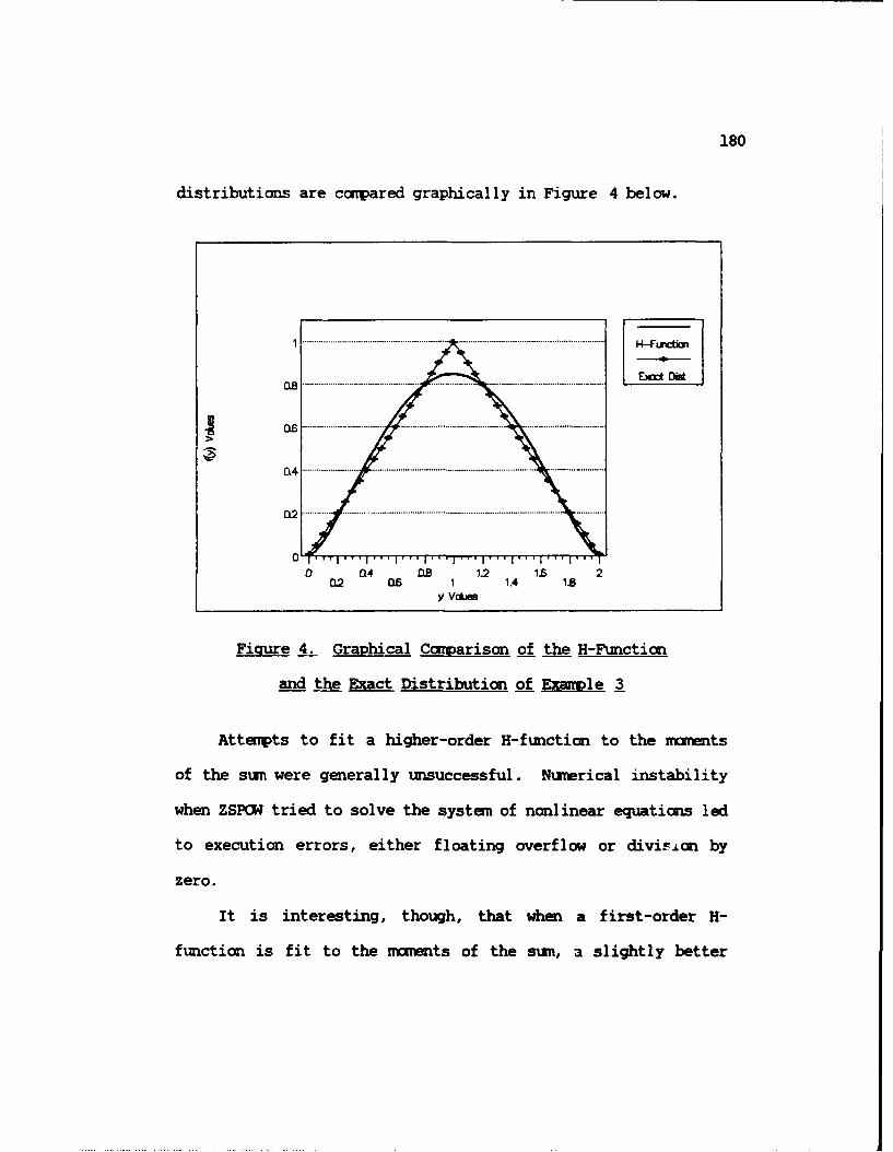
180

distributions are ccfqpared graphically in Figure 4 below.

1................... ..... . . . .rcb

Exar DsO .. ...... .. ............ - . . .-- * ---- - .

O ---- - ----- ..... .

CA .............4........ .......... . .. - .--------

0 04 O5 1.2 1.6 2a2 ftS 1 1.4 1is

y VC*J

Ficure 4. Graphical Convarison of the H-Function.

and the Exact Distribution of Exanyle 3

Attempts to fit a higher-order H-function to the rraTents

of the sum were generally unsuccessful. Nuerical instability

when ZSPOW tried to solve the system of nonlinear equations led

to execution errors, either floating overflow or division by

zero.

It is interesting, though, that when a first-order H-

function is fit to the ncinmts of the sun, a slightly better

181

fit is obtained, at least over the range of the variable fran

zero to two. The measures of merit were

Estinmted SSE = 0.0620352924

Estimated MSE = 0.0015508823

MAD = 0.1107462928

Estimted IADD = 0.0581953790

The drawback of this slightly better fit is that this H-

function distribution is positive for all y>0. At y=2.0, the

first-order H-function distribution has f(2)=.0348 and

F(2)=.9966. Therefore, the probability of achieving a value

greater than two with the first-order H-function distribution

is .0034. Of course, this event is impossible and the

probability should be zero. Most of the measures given above

would increase (worsen) if they were ccputed over a larger

range of the variable since the exact distribution has f(y)=0

for y>2 but the first-order H-function distribution has f(y)>O

for y>2.

5.3.4. EXAWLE 4 - SUM OF TWO INDEPEDET, IDENITICALLY

DISTRIBUTED BETM VARIATES

This exanple demonstrates the technique for the sum of two

Type VI convergent Hi 0 variates over (0,1) where the first

derivative of the exact distribution is continuous at y-1. The

exact distribution is given by Eq (5.17). Again, the nments

182

of the approximate H-function distribution were reasonably

close to those of the exact distribution. The measures of

merit were

Estimated SSE = 0.0358601689

Estimated MSE = 0.0008965042

MAD = 0.0579816425

Estimated IADD = 0.0442126253

The approximate H-function distribution more closely matched

the exact distribution than in the previous example, but not as

close as in the gamma and Erlang examples. While the two

functions which represent the exact distribution have a

continuous first derivative at y=I, the second derivative is

not continuous there. The approximate H-function distribution

has continuous derivatives of all orders for y E (0,2). The

two distributions are compared graphically in Figure 5 below.

183

12-4

E-FctiDn

0.2 0.6 1 1.4 1.8y Vdi

Fiqiure 5. Graphical Cavarison of the H-Ftmction

and the Exact Distribution of Examrl e 4

cOAPTER 6

OINCLUSIONS AND REOC4EDATIONS FOR FRfTHER STUDY

This thesis has presented a practical method to find an H-

function distribution for the sum of two or more independent H-

function variates. The method finds the noments about the

origin of each variate in the sum and uses these to find the

moments of the sum. The parameters of an H-function are then

estimated using the method of moments. This produces an H-

function distribution whose moments closely approximate those

of the sum of independent H-function variates.

The new technique is especially useful because the H-

function can exactly represent nearly every named statistical

distribution of positive random variables. By rewriting the

distributions of the random variables in the sum in their H-

function representations, an analyst can find the sum of two or

more independent variates with practically any distributional

form.

Further, simple formulas exist which immediately give the

distribution, as an H-function, of the random variable defined

as the product, quotient, or power of independent H-function

184

185

variates. The new technique for the sum allows an analyst to

exploit these powerful H-function results to find the H-

function distribution of more cumplicated algebraic

cumbinations of independent random variables.

When the exact distribution of an algebraic combination of

independent randum variables is difficult or impossible to

obtain, an analyst may resort to computer simulation to analyze

its distributional properties. The method presented here, when

cambined with the other H-function results, give an H-function

distribution for the algebraic combination, possibly precluding

the need to rely on ccuputer simulation.

A FORTRAN ccmputer program which implements the new

technique is demonstrated through five examples. Of course,

the program was also tested on many other examples. When it

was possible to find the exact distribution for the sum of

independent randam variables, the approximate H-function

distribution was ccMared to the exact distribution.

In cases where the exact distribution of the sum is widely

known (e.g. reproductive distributions), the method always

found the correct H-function representation for the sum. In

other cases, only the moments used to estimate the H-function

parameters agreed with those of the sum. Other, higher-order

mozents were in error to same degree. The method was less

186

effective in finding an H-function distribution which closely

approximated the exact distribution of the sum of independent

variates over a restricted range. These sums produce an exact

distribution with two functional forms over distinct ranges of

the variable and do not have continuous derivatives of all

orders at y-1.

The exact distribution of the general sum of independent

Erlang variates with different scale parameters, X, was derived

in Section 5.1.3. An Erlang variate is simply a gamma variate

with an integer shape parameter r. The derivation used partial

fractions to decompose the product of Laplace transforms of the

individual densities. This produced a sum of term, each of

which could easily be inverted from transform space, yielding

the desired density of the sun of independent variates.

Throughout the thesis, a number of other new results

relating to the H-function were given. A previously unstated

restriction on the variable in the H-function representations

of power functions and beta-type functions was highlighted.

Several ways of overconing this limitation when representing

mathematical functions were presented. These include scaling

the variable, allowing a slightly different function to be

represented for a range of the variable, or the use of couplex

parameters.

187

The restriction, however, is an advantage when

representing certain statistical distributions. For random

variables with a restricted range of the variable, the H-

function representation eliminates the need to specify the

range for which the den.sity is nonzero. The H-function

diss.-ibution exactly represents the desired density over the

appropriate range and is zero elsewhere.

Through scaling the variable of these H-functions with the

parameter c, the value where the H-function changes from

representing the special case to taking the value zero can be

changed. This allowed the H-function to represent the power

functions and beta-type functions over a more general range and

also gave the H-function representation of the Unit Step

Function and its complement. The same technique was used to

give the H-function representation of the Three-Parameter Beta

p.d.f., the Power Function p.d.f. over (0,M), the Uniform

p.d.f. over (0,M), and the Pareto p.d.f. over (cm).

Analytic solutions were derived for the system of

nonlinear equations generated by the method of moments to

estimate the H-function parameters for certain distributions.

These distributions have restricted ranges of the variable and

must be represented by Type VI convergent H-functions.

Many new H-function representations of other mathematical

188

functions were also given, including those of the copleientary

error function, erfc x, the complementary incomplete gain,

function, r(a,x), the complementary incomplete beta function,

Bx(a,P), and the inverse hyperbolic cotangent function,

arccoth z.

Four new theorem show when and how a generalizing

constant rmy be present in an H-function representation. Many

generalized H-function representations are given, including

those of every cumulative distribution function of an H-

function variate. The generalizing constant was also possible

in the H-function representations of power functions, the error

function and its complenent, the incorrplete ganma function and

its complement, the incomplete beta function and its

cornlement, nany inverse trigonometric and hyperbolic

functions, and the logarithnic functions.

Sufficient convergence conditions were developed for the

alternate definition of the H-function. These show where the

H-function rmy be evaluated by the sum of LHP residues or the

negative sum of RHP residues, without first changing the form

of the alternate definition of the H-function to that of the

prirmry definition.

The hierarchical structure among classes of H-functions

was given through seven new theorem. Every class of H-

189

functions is wholly contained in many higher-order classes of

H-functions through the application of the duplication,

triplication, and multiplication formulas for the ganna

function. In the other direction, the hierarchical structure

gives new reduction properties that are less obvious than the

known reduction properties.

Several new results were obtained for powers of first-

order H-function variates. The square of a random variable

with a Rayleigh distribution with parameter X has an

exponential distribution with parameter X. If X has a Weibull

distribution with parameters P and X, then Y=X where P>O has a

Weibull distribution with parameters -1 and X. The square of

a randn variable with a half-norual distribution with

1parameter a has a gaima distribution with parameters r -

and X 2 . The square of a randm variable with a Maxwell

distribution with parameter 8 has a gamrm distribution with

3 1parameters r = and X = =. The square of a random

variable with a Maxwell distribution with parameter 8 = has

a Chi-Square distribution with parameter P=3. The square of a

random variable with a Rayleigh distribution with parameter1

X has a Chi-Square distribution with parameter v=2.

Many areas of further research proposed by Eldred (1979,

190

pp. 258-9], Cook [1981, pp. 145-147], Kellogg [1984, pp.1 7 0-

171], and Jacobs (1986, pp. 149-152] remain unfinished.

Readers interested in H-function research should consider those

recommendations and same additional areas that follow.

In Bayesian statistics, the parameters of a distribution

are considered to be random variables with a particular

distribution. After sampling from the distribution, the

information gained about the parameters is reflected by

updating the prior distribition and creating a posterior

distribution. To my knowledge, a Bayesian approach has not

been attempted with the H-function.

Numerical methods exist for certain commonly-used

transforms such as the Laplace and Fourier transforms. If

these methods are sufficiently accurate and will work in both

directions (finding a transform and inverting a transform), it

would be possible to find the distribution (in tabular form) of

sums or differences of independent random variables. If a

numerical method to invert a Mellin transform exists, it could

be used to evaluate the H-function.

The computer program by Cook [1981, Cook and Barnes, 1981]

will evaluate an H-function by the sum of residues for certain

values of the real variable, x, when given the parameters of

the H-function. The program's capabilities should be extended

191

to allow complex parameters of the H-function and to evaluate

the H-function at values of the conrplex variable, z.

The numerical solution of the systen of nonlinear

equations with ZSPCW is sometimes numerically unstable.

Several other numerical methods were tried, but none worked as

well as ZSPCW in solving the type of nonlinear equations

generated using the method of noments with the H-function.

Further research might develop a better way to solve the system

of nonlinear equations.

While the H-function has been shown to exactly represent

many mathematical functions and statistical distributions,

there are a few functions and distributions which have not yet

been shown to be H-functions. Conversely, no one has proven

that these functions cannot be represented as H-functions.

Examples include the gamma function, certain trigonmcetric and

hyperbolic functions, and the Lognormal and Logistic densities.

A related issue is to prove or disprove that the product of two

H-functions is another H-function.

To my knowledge, the H-function has not been applied to

the study of ccmplex-valued random variables. The H-function

sees the appropriate tool to analyze random variables which

take values in the complex plane.

The relationship between the H-function and the infinite

192

summbility of integrals described in Section 2.7 needs to be

mre extensively studied. Is there a particular summability

scheme the H-function always follows to obtain the moments of

the functions representable as H-functions?

Theorems similar to those in Section 2.4.6 could be

developed to show upgrade and reduction results for H-functions

by applying the triplication and multiplication formulas for

the gamm function. Then, the search could begin for a class

of H-functions which includes most of the known special cases.

For example, Figure 1 showed the H. 0 class includes many1 1

common statistical distributions, including all those in the

H' 0 class. The half-Cauchy, half-Student, and F1

distributions, however, are in the H' 1 class of H-function1 1

distributions. Using combinations of theorems based on the

duplication, triplication, or multiplication formulas, is there

a class of H-functions which includes both the H' 0 and H' 111 11

classes of H-functions?

The H-function continues to be an extremely rewarding area

of research for me. I am convinced that we have much to

discover about its ability to simplify many difficult problems

in mathematics, probability, and statistics. Those who pursue

H-function research should find it both challenging and

rewarding.

APPEDIX A

OUTPUT FRO4 CCPUTER PROGRAMS

Listed below are the complete output files from the

FORTRAN computer programs for each of the five examples in

Section 4.4. The output fran the program which finds a H-

function distribution for the sum of independent H-function

variates is followed by the output from a different program

[Cook, 1981; Cook and Barnes, 1981) which evaluates the p.d.f.

and c.d.f. of the resulting H-function distribution. For the

first four examples for which it was possible to find the exact

distribution, the output from the program which carpares the

approximate H-function distribution to the exact distribution

is also presented.

EXAMPLE 1 - SUN OF THREE INDEPIMET, IDENTICALLY

DISTRIBUTED GAM4A VARIATES

PROGRAM SUKVAR RUN IN DIBLE PRECISIONFOR THE SUM OF 3 INDEPENDENT H-FUNCTION VARIATESINPUT PARAMETERS FOR VARIABLE NMB 1 OF THE SUM:

M, N, P,Q = 1 0 0 1K, C = 2.0000000 2.0000000b, B = 1.00000 1.00000THE MCHETS ABOUT THE ORIGIN ARE:

THE ZEROTH MI.N T IS 1.0000000THE FIRST M34MT IS 1.0000000

193

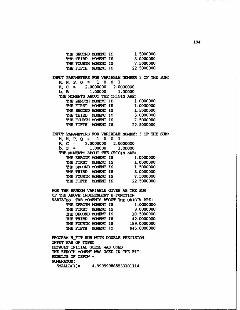
194

THE SECIND MOMET IS 1.5000000THE THIRD MOMENT IS 3.0000000THE FOURTH MOMENT IS 7.5000000THE FIFTH MOMENT IS 22.5000000

INPUT PARAETES FOR VARIABLE NUBER 2 OF THE S,]:M, N, P, Q = 1 0 0 1K, C = 2.0000000 2.0000000b, B = 1.00000 1.00000THE MMTS ABOUT THE ORIGIN ARE:

THE ZEROTH MOMENT IS 1.0000000THE FIRST MOMENT IS 1.0000000THE SECOND MOM ENT IS 1.5000000THE THIRD MOMENT IS 3.0000000THE FURTH MOMT IS 7.5000000THE FIFTH MDENT IS 22.5000000

INPUT PARAMETERS FOR VARIABLE NUMBER 3 OF THE SU4:M, N, P, Q = 1 0 0 1K, C = 2.0000000 2.0000000b, B = 1.00000 1.00000THE MOMENT S ABOY THE ORIGIN ARE:

THE ZEROTH MMENT IS 1.0000000THE FIRST MOMENT IS 1.0000000THE SECOND MOMENT IS 1.5000000THE THIRD MOMENT IS 3.0000000THE FOURTH MOMENT IS 7.5000000THE FIFTH MOMENT IS 22.5000000

FOR THE RANDCM VARIABLE GIVEN AS THE SMOF THE ABOVE INDEPENDENT H-FUNCTICtVARIATES, THE MOMEMTS ABOUT THE ORIGIN ARE:

THE ZEFDTH MOMENT IS 1.0000000THE FIRST MOMENT IS 3.0000000THE SEOOND MOMENT IS 10.5000000THE THIRD MOMENT IS 42.0000000THE FOURTH MOMENT IS 189.0000000THE FIFTH MOMENT IS 945.0000000

PROGRAM HFIT RUN WITH DOUBLE PRECISIONINPUT WAS OF TYPEODEFAULT INITIAL GUESS WAS USEDTHE ZETH MOMENT WAS USED IN THE FITRESULTS OF ZSPOW -NUERAT(R:

SMALLB(1)= 4.999999888533181114

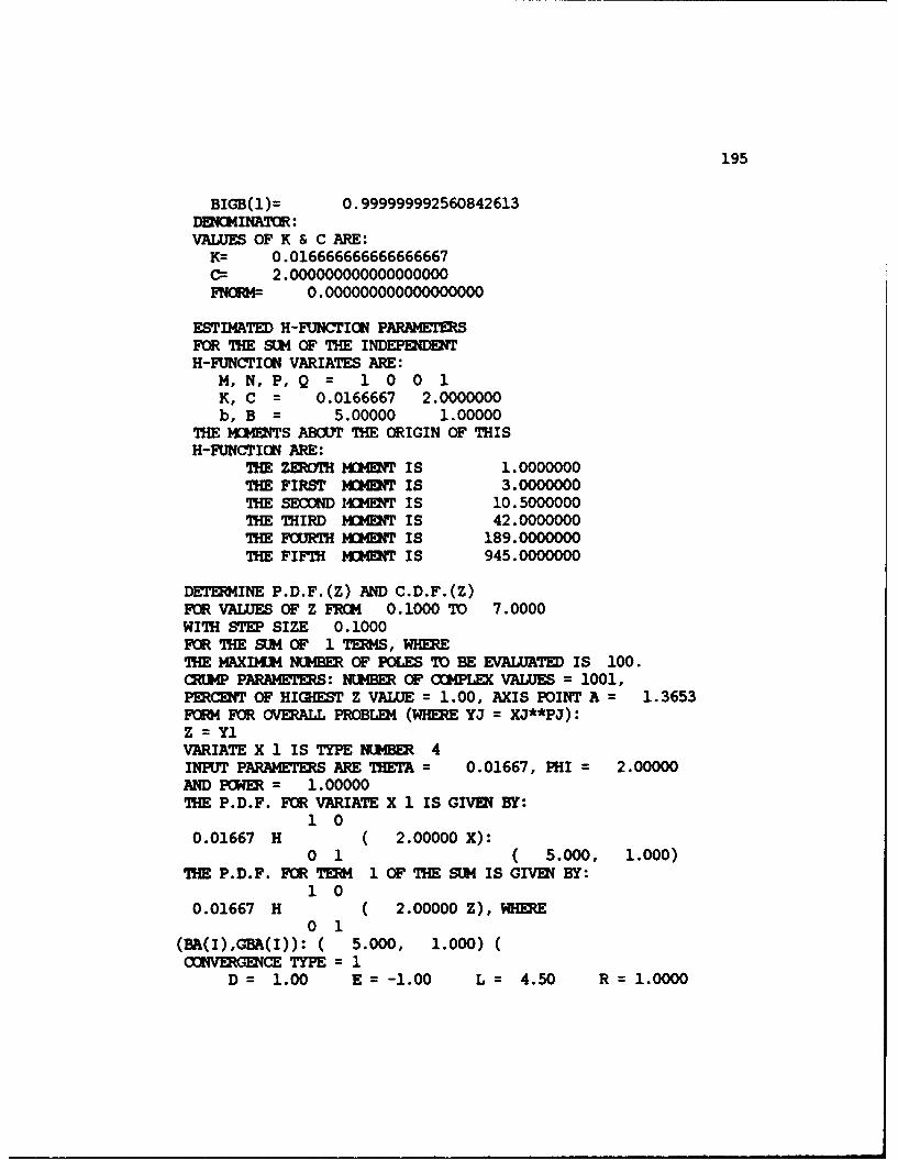
195

BIGB(1)= 0.999999992560842613DENC14INATOR:VALUES OF K & C ARE:K- 0.016666666666666667C 2.000000000000000000FNIORM= 0.000000000000000000

ESTIMATED H-FUNCTICt PARAMETERSFOR THE SU OF THE INDEPENDENTH-FUNCTICO VARIATES ARE:

M, N, P, Q = 1 0 0 1K, C = 0.0166667 2.0000000b, B = 5.00000 1.00000

THE MOIETS ABOUT THE ORIGIN OF THISH-FUNCTION ARE:

THE ZEROTH MOMENT IS 1.0000000THE FIRST IIMTM IS 3.0000000THE SECIOND 14HM IS 10.5000000THE THIRD MOMENT IS 42.0000000THE FOURTH MOMHDT IS 189.0000000THE FIFTH M(MOIT IS 945.0000000

DETERMINE P.D.F.(Z) AND C.D.F.(Z)FO VALUES OF Z FRCM 0.1000 TO 7.0000WITH STEP SIZE 0.1000FOR THE SU14 OF 1 TERKS, WHERETHE MAXIMU4 NUMBER OF POLES TO BE EVALUATED IS 100.CRIMP PARAMETERS: NUMBER OF CC)(PLEX VALUES = 1001,PERCEIT OF HIGHEST Z VALUE = 1.00, AXIS POINT A = 1.3653FUN FOR OVERALL PROBLEM (WHERE YJ = XJ**PJ):Z = YIVARIATE X 1 IS TYPE NUMBER 4INPUT PARAMETERS ARE THETA = 0.01667, PHI - 2.00000AND POWER - 1.00000THE P.D.F. FOR VARIATE X 1 IS GIVEN BY:

1 00.01667 H ( 2.00000 X):

0 1 ( 5.000, 1.000)THE P.D.F. FUR TERM 1 OF THE SUK IS GIVENi BY:

1 00.01667 H ( 2.00000 Z), WHE

0 1(BA(I),GBA(1)): ( 5.000, 1.000) (COVERGENCE TYPE = 1

D = 1.00 E = -1.00 L= 4.50 R = 1.0000

196

z PDF(Z) CDF(Z)0.1000 0.000004 0.0000000.2000 0.000114 0.0000040.3000 0.000711 0.0000390.4000 0.002454 0.0001840.5000 0.006131 0.0005940.6000 0.012491 0.0015000.7000 0.022104 0.0032010.8000 0.035284 0.0060400.9000 0.052057 0.0103781.0000 0.072179 0.0165641.1000 0.095173 0.0249101.2000 0.120392 0.0356731.3000 0.147079 0.0490371.4000 0.174427 0.0651101.5000 0.201638 0.0839181.6000 0.227959 0.1054081.7000 0.252721 0.1294581.8000 0.275360 0.1558811.9000 0.295425 0.1844442.0000 0.312587 0.2148702.1000 0.326632 0.2468572.2000 0.337455 0.2800882.3000 0.345051 0.3142402.4000 0.349495 0.3489942.5000 0.350935 0.3840392.6000 0.349570 0.4190872.7000 0.345643 0.4538682.8000 0.339422 0.4881392.9000 0.331193 0.5216853.0000 0.321246 0.5543203.1000 0.309871 0.5858873.2000 0.297347 0.6162563.3000 0.283939 0.6453273.4000 0.269892 0.6730233.5000 0.255433 0.6992923.6000 0.240764 0.7241023.7000 0.226062 0.7474433.8000 0.211484 0.7693193.9000 0.197163 0.7897494.0000 0.183207 0.8087644.1000 0.169708 0.8264054.2000 0.156737 0.8427234.3000 0.144347 0.8577724.4000 0.132578 0.8716134.5000 0.121454 0.884309

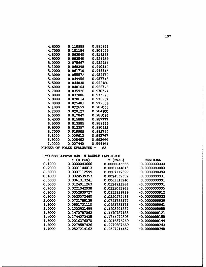
197

4.6000 0.110989 0.8959264.7000 0.101186 0.9065294.8000 0.092040 0.9161854.9000 0.083540 0.9249595.0000 0.075667 0.9329145.1000 0.068398 0.9401125.2000 0.061710 0.9466135.3000 0.055572 0.9524725.4000 0.049956 0.9577455.5000 0.044830 0.9624805.6000 0.040164 0.9667265.7000 0.035926 0.9705275.8000 0.032086 0.9739255.9000 0.028614 0.9769576.0000 0.025481 0.9796596.1000 0.022659 0.9820636.2000 0.020123 0.9842006.3000 0.017847 0.9860966.4000 0.015808 0.9877776.5000 0.013985 0.9892656.6000 0.012357 0.9905816.7000 0.010905 0.9917426.8000 0.009612 0.9927676.9000 0.008462 0.9936697.0000 0.007440 0.994464

NUMBE OF POLES EVALUATED = 83

PROGRAM CCHPAR RUN IN DOUBLE PRECISIONx Y (H-FCN) Y (EVAL) RESIDUAL

0.1000 0.0000043666 0.0000043666 0.00000000000.2000 0.0001144013 0.0001144013 0.00000000000.3000 0.0007112599 0.0007112599 0.00000000000.4000 0.0024539353 0.0024539352 0.00000000010.5000 0.0061313241 0.0061313240 0.00000000010.6000 0.0124911263 0.0124911264 -0.00000000010.7000 0.0221042938 0.0221042943 -0.00000000050.8000 0.0352839727 0.0352839739 -0.00000000120.9000 0.0520572460 0.0520572483 -0.00000000231.0000 0.0721788138 0.0721788177 -0.00000000391.1000 0.0951731110 0.0951731171 -0.00000000611.2000 0.1203921499 0.1203921587 -0.00000000881.3000 0.1470787062 0.1470787183 -0.00000001211.4000 0.1744272435 0.1744272593 -0.00000001581.5000 0.2016376070 0.2016376269 -0.00000001991.6000 0.2279587426 0.2279587669 -0.00000002431.7000 0.2527214162 0.2527214452 -0.0000000290

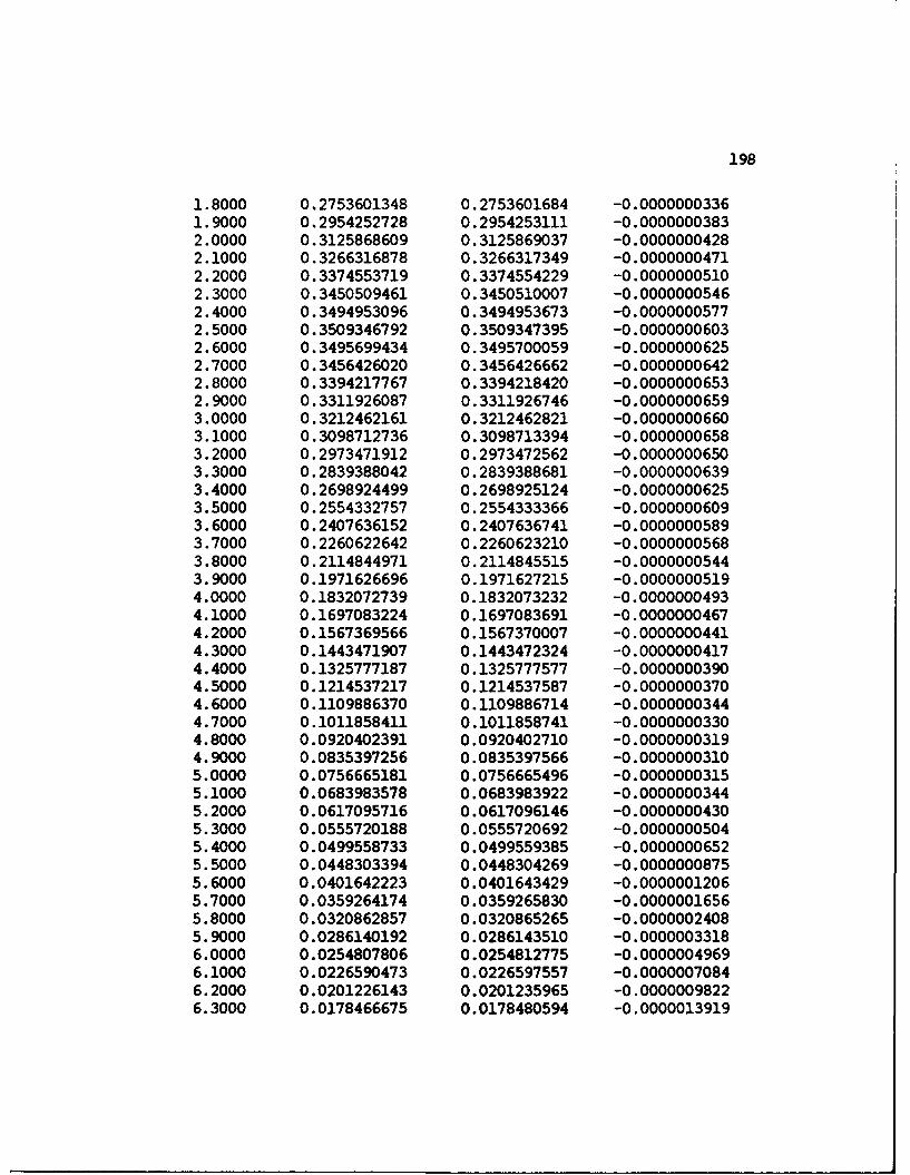
198

1.8000 0.2753601348 0.2753601684 -0.00000003361.9000 0.2954252728 0.2954253111 -0.00000003832.0000 0.3125868609 0.3125869037 -0.00000004282.1000 0.3266316878 0.3266317349 -0.00000004712.2000 0.3374553719 0.3374554229 -0.00000005102.3000 0.3450509461 0.3450510007 -0.00000005462.4000 0.3494953096 0.3494953673 -0.00000005772.5000 0.3509346792 0.3509347395 -0.00000006032.6000 0.3495699434 0.3495700059 -0.00000006252.7000 0.3456426020 0.3456426662 -0.00000006422.8000 0.3394217767 0.3394218420 -0.00000006532.9000 0.3311926087 0.3311926746 -0.00000006593.0000 0.3212462161 0.3212462821 -0.00000006603.1000 0.3098712736 0.3098713394 -0.00000006583.2000 0.2973471912 0.2973472562 -0.00000006503.3000 0.2839388042 0.2839388681 -0.00000006393.4000 0.2698924499 0.2698925124 -0.00000006253.5000 0.2554332757 0.2554333366 -0.00000006093.6000 0.2407636152 0.2407636741 -0.00000005893.7000 0.2260622642 0.2260623210 -0.00000005683.8000 0.2114844971 0.2114845515 -0.00000005443.9000 0.1971626696 0.1971627215 -0.00000005194.0000 0.1832072739 0.1832073232 -0.00000004934.1000 0.1697083224 0.1697083691 -0.00000004674.2000 0.1567369566 0.1567370007 -0.00000004414.3000 0.1443471907 0.1443472324 -0.00000004174.4000 0.1325777187 0.1325777577 -0.00000003904.5000 0.1214537217 0.1214537587 -0.00000003704.6000 0.1109886370 0.1109886714 -0.00000003444.7000 0.1011858411 0.1011858741 -0.00000003304.8000 0.0920402391 0.0920402710 -0.00000003194.9000 0.0835397256 0.0835397566 -0.00000003105.0000 0.0756665181 0.0756665496 -0.00000003155.1000 0.0683983578 0.0683983922 -0.00000003445.2000 0.0617095716 0.0617096146 -0.00000004305.3000 0.0555720188 0.0555720692 -0.00000005045.4000 0.0499558733 0.0499559385 -0.00000006525.5000 0.0448303394 0.0448304269 -0.00000008755.6000 0.0401642223 0.0401643429 -0.00000012065.7000 0.0359264174 0.0359265830 -0.00000016565.8000 0.0320862857 0.0320865265 -0.00000024085.9000 0.0286140192 0.0286143510 -0.00000033186.0000 0.0254807806 0.0254812775 -0.00000049696.1000 0.0226590473 0.0226597557 -0.00000070846.2000 0.0201226143 0.0201235965 -0.00000098226.3000 0.0178466675 0.0178480594 -0.0000013919

199

6.4000 0.0158078894 0.0158099039 -0.00000201456.5000 0.0139846566 0.0139874081 -0.00000275156.6000 0.0123566022 0.0123603635 -0.00000376136.7000 0.0109048623 0.0109100486 -0.00000518636.8000 0.0096119998 0.0096191863 -0.00000718656.9000 0.0084623041 0.0084718905 -0.00000958647.0000 0.0074402961 0.0074536017 -0.0000133056ESTIMATED SSE IS 0.0000000004ESTIMATED MSE IS 0.0000000000THE MAXIMUM ABSOLUTE DIFF CE BENEEN THEH-FUNCTION AND THE ACTUAL FUNCTION IS 0.0000133056THE INTEGRATED ABSOLUTE DENSITY DIFFERENCE(AN ESTIMATE OF THE AREA BEFEWE THEH-FUNCTION AND THE ACTUAL DENSITY) IS 0.0000050304

EXAMPLE 2 - SUM OF TWO INDEPEDENT ERLANG VARIATES

WITH DIFFERENT X

PROGRAM SUMVAR RUN IN DOUBLE PRECISIONFOR THE SUM OF 2 INDEPE DEN T H-FUNCTION VARIATESINPUT PARAMETERS FOR VARIABLE NUMBER 1 OF THE SUM:

M, N, P, Q = 1 0 0 1K, C = 4.0000000 4.0000000b, B = 1.00000 1.00000THE MOKMNTS ABOUT THE ORIGIN ARE:

THE ZEROTH MOMENT IS 1.0000000THE FIRST MCMET IS 0.5000000THE SECOND MCDEIT IS 0.3750000THE THIRD MOMENT IS 0.3750000THE FOURTH M(CMET IS 0.4687500THE FIFTH MCME2 T IS 0.7031250THE NEXT M(MENT IS 1.2304688THE NEXT MD4DIT IS 2.4609375

INPUT PARAMETERS FOR VARIABLE NUMBER 2 OF THE SU4:M, N, P,Q = 1 0 0 1K, C = 2.0000000 2.0000000b, B = 0.00000 1.00000THE MGM]VTS ABOUT THE ORIGIN ARE:

THE ZEROTH MCMT IS 1.0000000THE FIRST MOMEIT IS 0.5000000THE SECOND MOMENT IS 0.5000000THE THIRD MlCMKWT IS 0.7500000

200

THE FOURTH MOMENT IS 1.5000000THE FIFTH MOMENT IS 3.7500000THE NEXT MOMENT IS 11.2500000THE NEXT MOMENT IS 39.3750000

FOR THE RANDI4 VARIABLE GIVEN AS THE SLIMOF THE ABOVE INDEPENDEIT H-FUNCTIONVARIATES, THE MO4TS ABOUT THE ORIGIN ARE:

THE ZROIH MOM]ENT IS 1.0000000THE FIRST MMENT IS 1.0000000THE SECOND MOMENT IS 1.3750000THE THIRD MOMEIT IS 2.4375000THE FOURTH MOMENT IS 5.3437500THE FIFTH MCME 4T IS 14.0625000THE NEXT MOMENT IS 43.4179688THE NEXT MOMENT IS 154.4238281

PROGRAM H_FIT RUN WITH DOUBLE PRECISIONINPUT WAS OF TYPEDEFAULT INITIAL GUESS WAS USEDTHE ZEROTH MDMENT WAS USED IN THE FITRESULTS OF ZSPCN -NUMRAATOR:

SMALLB(1)= 3.024855875185841148BIGB(1)= 1.263891763119380202

DENCMINATOR:VALUES OF K & C ARE:

K= 0.748958966084013356C 6.533302402015585986FNORM= 0.000000000000000000

ESTIMATED H-FUNCTION PARAMET SFOR THE SUM OF THE INDEPENDENTH-FUNCTION VARIATES ARE:

M, N, P,Q = 1 0 0 1K, C = 0.7489590 6.5333024b, B = 3.02486 1.26389

THE MM40TS ABOUT THE ORIGIN OF THISH-FUNCTION ARE:

THE ZEROTH OMENT IS 1.0000000THE FIRST MCMET IS 1.0000000THE SECOND MO4ENT IS 1.3750000THE THIRD MO4EIT IS 2.4375000THE FOURTH MiEMT IS 5.3382458THE FIFTH MCMENT IS 14.0112602THE NEXT MOMEIT IS 43.0835662

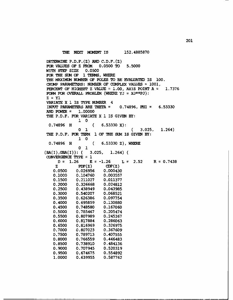
201

THE NEXT MOMENT IS 152.4885870

DETERMINE P.D.F.(Z) AND C.D.F.(Z)FOR VALUES OF Z FROM 0.0500 TO 5.5000WITH STEP SIZE 0.0500FOR THE SUM OF 1 TERMS, WHERETHE MAXIMUM NUMBER OF POLES TO BE EVALUATED IS 100.CRUMP PARAMEIERS: NUMBER OF COMPLEX VALUES = 1001,PERCENT OF HIGHEST Z VALUE = 1.00, AXIS POINT A 1.7376FORM FOR OVERALL PROBLEM (WHERE YJ = XJ**PJ):Z = YIVARIATE X 1 IS TYPE NUMBER 4INPUT PARAMETERS ARE THETA = 0.74896, PHI = 6.53330AND POWER = 1.00000THE P.D.F. FOR VARIATE X 1 IS GIVEN BY:

1 00.74896 H ( 6.53330 X):

0 1 ( 3.025, 1.264)THE P.D.F. FOR TERM 1 OF THE SUM IS GIVEN BY:

1 00.74896 H ( 6.53330 Z), WHERE

0 1(BA(I),GBA(I)): ( 3.025, 1.264) (ONVERGENCE TYPE = 1

D = 1.26 E = -1.26 L = 2.52 R = 0.7438Z PDF(Z) CDF(Z)

0.0500 0.026956 0.0004300.1000 0.104760 0.0035570.1500 0.211027 0.0113770.2000 0.326668 0.0248120.2500 0.438949 0.0439850.3000 0.540207 0.0685210.3500 0.626386 0.0977540.4000 0.695859 0.1308800.4500 0.748580 0.1670600.5000 0.785467 0.2054740.5500 0.807989 0.2453670.6000 0.817884 0.2860630.6500 0.816969 0.3269750.7000 0.807023 0.3676090.7500 0.789713 0.4075550.8000 0.766559 0.4464830.8500 0.738910 0.4841360.9000 0.707945 0.5203190.9500 0.674675 0.5548921.0000 0.639955 0.587762

202

1.0500 0.604498 0.6188751.1000 0.568889 0.6482101.1500 0.533601 0.6757701.2000 0.499009 0.7015811.2500 0.465403 0.7256871.3000 0.433003 0.7481421.3500 0.401967 0.7690101.4000 0.372404 0.7883631.4500 0.344381 0.8062761.5000 0.317931 0.8228271.5500 0.293060 0.8380961.6000 0.269752 0.8521591.6500 0.247973 0.8650961.7000 0.227679 0.8769811.7500 0.208814 0.8878881.8000 0.191315 0.8978861.8500 0.175116 0.9070411.9000 0.160147 0.9154181.9500 0.146338 0.9230752.0000 0.133618 0.9300702.0500 0.121917 0.9364542.1000 0.111168 0.9422772.1500 0.101305 0.94752152.2000 0.092263 0.9524212.2500 0.083984 0.9568242.3000 0.076410 0.9608312.3500 0.069486 0.9644762.4000 0.063163 0.9677902.4500 0.057391 0.9708022.5000 0.052127 0.9735382.5500 0.047330 0.9760222.6000 0.042959 0.9782782.6500 0.038980 0.9803252.7000 0.035359 0.9821822.7500 0.032066 0.9838662.8000 0.029072 0.9853932.8500 0.026351 0.9867782.9000 0.023880 0.9880332.9500 0.021636 0.9891703.0000 0.019599 0.9902003.0500 0.017751 0.9911333.1000 0.016074 0.9919783.1500 0.014553 0.9927433.2000 0.013174 0.9934353.2500 0.011924 0.9940623.3000 0.010792 0.994630

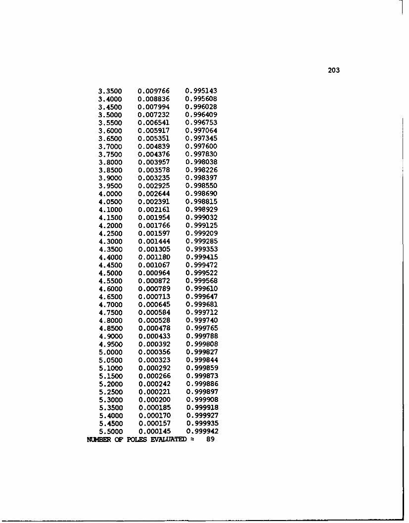
203

3.3500 0.009766 0.9951433.4000 0.008836 0.9956083.4500 0.007994 0.9960283.5000 0.007232 0.9964093.5500 0.006541 0.9967533.6000 0.005917 0.9970643.6500 0.005351 0.9973453.7000 0.004839 0.9976003.7500 0.004376 0.9978303.8000 0.003957 0.9980383.8500 0.003578 0.9982263.9000 0.003235 0.9983973.9500 0.002925 0.9985504.0000 0.002644 0.9986904.0500 0.002391 0.9988154.1000 0.002161 0.9989294.1500 0.001954 0.9990324.2000 0.001766 0.9991254.2500 0.001597 0.9992094.3000 0.001444 0.9992854.3500 0.001305 0.9993534.4000 0.001180 0.9994154.4500 0.001067 0.9994724.5000 0.000964 0.9995224.5500 0.000872 0.9995684.6000 0.000789 0.9996104.6500 0.000713 0.9996474.7000 0.000645 0.9996814.7500 0.000584 0.9997124.8000 0.000528 0.9997404.8500 0.000478 0.9997654.9000 0.000433 0.9997884.9500 0.000392 0.9998085.0000 0.000356 0.9998275.0500 0.000323 0.9998445.1000 0.000292 0.9998595.1500 0.000266 0.9998735.2000 0.000242 0.9998865.2500 0.000221 0.9998975.3000 0.000200 0.9999085.3500 0.000185 0.9999185.4000 0.000170 0.9999275.4500 0.000157 0.9999355.5000 0.000145 0.999942

NUMBER OF POLES EVALUATED 89

204

PROGRAM COMPAR RUN IN DCUBLE PRECISIONx Y (H-FCN) Y (EVAL) RESIDUAL

0.0500 0.0269560422 0.0338687172 -0.00691267500.1000 0.1047604975 0.1147735827 -0.01001308520.1500 0.2110272898 0.2189047501 -0.00787746030.2000 0.3266679624 0.3300759702 -0.00340800780.2500 0.4389488040 0.4376919836 0.00125682040.3000 0.5402072867 0.5352071763 0.00500011040.3500 0.6263855876 0.6189637207 0.00742186690.4000 0.6958594647 0.6873218538 0.00853761090.4500 0.7485799015 0.7400141770 0.00856572450.5000 0.7854665809 0.7776709976 0.00779558330.5500 0.8079891806 0.8014756091 0.00651357150.6000 0.8178843945 0.8129177174 0.00496667710.6500 0.8169693788 0.8136205051 0.00334887370.7000 0.8070228765 0.8052225091 0.00180036740.7500 0.7897133043 0.7892999138 0.00041339050.8000 0.7665590050 0.7673183012 -0.00075929620.8500 0.7389101583 0.7406055613 -0.00169540300.9000 0.7079449386 0.7103397230 -0.00239478440.9500 0.6746747268 0.6775470467 -0.00287231991.0000 0.6399547674 0.6431069326 -0.00315216521.0500 0.6044977968 0.6077611209 -0.00326332411.1000 0.5688889715 0.5721253654 -0.00323639391.1500 0.5336009937 0.5367022861 -0.00310129241.2000 0.4990087333 0.5018945066 -0.00288577331.2500 0.4654029237 0.4680174730 -0.00261454931.3000 0.4330027002 0.4353115704 -0.00230887021.3500 0.4019668816 0.4039533060 -0.00198642441.4000 0.3724039823 0.3740654440 -0.00166146171.4500 0.3443809949 0.3457260524 -0.00134505751.5000 0.3179310207 0.3189764773 -0.00104545661.5500 0.2930598403 0.2938282943 -0.00076845401.6000 0.2697515271 0.2702693074 -0.00051778031.6500 0.2479732076 0.2482686787 -0.00029547111.7000 0.2276790667 0.2277812745 -0.00010220781.7500 0.2088136949 0.2087513166 0.00006237831.8000 0.1913148623 0.1911154218 0.00019944051.8500 0.1751157994 0.1748051079 0.00031069151.9000 0.1601470554 0.1597488398 0.00039821561.9500 0.1463379965 0.1458736804 0.00046431612.0000 0.1336179992 0.1331066060 0.00051139322.0500 0.1219173875 0.1213755376 0.00054184992.1000 0.1111681551 0.1106101339 0.00055802122.1500 0.1013045089 0.1007423864 0.00056212252.2000 0.0922632656 0.0917070504 0.0005562152

205

2.2500 0.0839841259 0.0834419409 0.00054218502.3000 0.0764098507 0.0758881208 0.00052172992.3500 0.0694863578 0.0689899994 0.00049635842.4000 0.0631627543 0.0626953630 0.00046739132.4500 0.0573913195 0.0569553491 0.00043597042.5000 0.0521274483 0.0517243794 0.00040306892.5500 0.0473295640 0.0469600610 0.00036950302.6000 0.0429590129 0.0426230642 0.00033594872.6500 0.0389799364 0.0386769844 0.00030295202.7000 0.0353591407 0.0350881930 0.00027094772.7500 0.0320659524 0.0318256831 0.00024026932.8000 0.0290720785 0.0288609122 0.00021116632.8500 0.0263514586 0.0261676457 0.00018381292.9000 0.0238801228 0.0237218028 0.00015832002.9500 0.0216360554 0.0215013070 0.00013474843.0000 0.0195990566 0.0194859415 0.00011311513.0500 0.0177506130 0.0176572119 0.00009340113.1000 0.0160737745 0.0159982144 0.00007556013.1500 0.0145530391 0.0144935125 0.00005952663.2000 0.0131742345 0.0131290204 0.00004521413.2500 0.0119244243 0.0118918938 0.00003253053.3000 0.0107918007 0.0107704277 0.00002137303.3500 0.0097656028 0.0097539623 0.00001164053.4000 0.0088360115 0.0088327943 0.00000321723.4500 0.0079940810 0.0079980955 -0.00000401453.5000 0.0072316960 0.0072418379 -0.00001014193.5500 0.0065414505 0.0065567237 -0.00001527323.6000 0.0059166029 0.0059361217 -0.00001951883.6500 0.0053510603 0.0053740084 -0.00002294813.7000 0.0048392420 0.0048649142 -0.00002567223.7500 0.0043761116 0.0044038736 -0.00002776203.8000 0.0039570862 0.0039863804 -0.00002929423.8500 0.0035779964 0.0036083458 -0.00003034943.9000 0.0032350765 0.0032660609 -0.00003098443.9500 0.0029249240 0.0029561618 -0.00003123784.0000 0.0026444213 0.0026755985 -0.00003117724.0500 0.0023907019 0.0024216056 -0.00003090374.1000 0.0021613239 0.0021916766 -0.00003035274.1500 0.0019539329 0.0019835396 -0.00002960674.2000 0.0017664002 0.0017951361 -0.00002873594.2500 0.0015968516 0.0016246006 -0.00002774904.3000 0.0014436486 0.0014702432 -0.00002659464.3500 0.0013051134 0.0013305330 -0.00002541964.4000 0.0011798299 0.0012040833 -0.00002425344.4500 0.0010667957 0.0010896381 -0.00002284244.5000 0.0009643209 0.0009860600 -0.0000217391

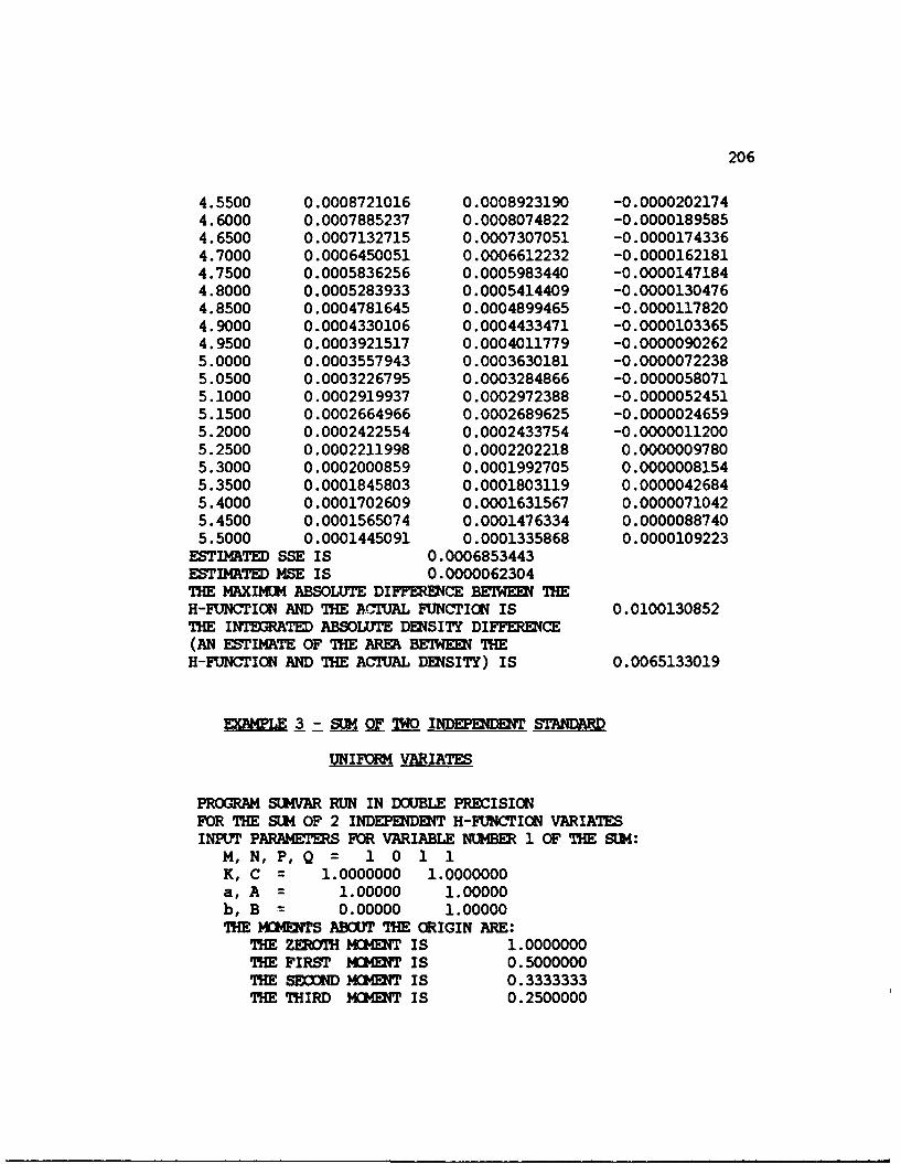
206

4.5500 0.0008721016 0.0008923190 -0.00002021744.6000 0.0007885237 0.0008074822 -0.00001895854.6500 0.0007132715 0.0007307051 -0.00001743364.7000 0.0006450051 0.0006612232 -0.00001621814.7500 0.0005836256 0.0005983440 -0.00001471844.8000 0.0005283933 0.0005414409 -0.00001304764.8500 0.0004781645 0.0004899465 -0.00001178204.9000 0.0004330106 0.0004433471 -0.00001033654.9500 0.0003921517 0.0004011779 -0.00000902625.0000 0.0003557943 0.0003630181 -0.00000722385.0500 0.0003226795 0.0003284866 -0.00000580715.1000 0.0002919937 0.0002972388 -0.00000524515.1500 0.0002664966 0.0002689625 -0.00000246595.2000 0.0002422554 0.0002433754 -0.00000112005.2500 0.0002211998 0.0002202218 0.00000097805.3000 0.0002000859 0.0001992705 0.00000081545.3500 0.0001845803 0.0001803119 0.00000426845.4000 0.0001702609 0.0001631567 0.00000710425.4500 0.0001565074 0.0001476334 0.00000887405.5000 0.0001445091 0.0001335868 0.0000109223

ESTIMATED SSE IS 0.0006853443ESTIMATE MSE IS 0.0000062304THE MAXIMUM ABSOLUTE DIFFERENCE BEDOW THEH-FUNCTION AND THE A.(7UAL FNCTION IS 0.0100130852THE INTEGRATED ABSOLUTE DEISITY DIFFERENCE(AN ESTIMATE OF THE AREA BE1WEEN THEH-FUNCTION AND THE ACI'UAL DEISITY) IS 0.0065133019

EXAMPLE 3 - SU14 OF TWO INDEPENDENT STANDARD

UNIFORM VARIATES

PROGRAM SUMVAR RUN IN DOUBLE PRECISIONFOR THE SU14 OF 2 INDEPEDENIT H-FUNCTION VARIATESINPUT PARAMETERS FOR VARIABLE NUMBER 1 OF THE S13:

M, N, P,Q = 1 0 1 1K, C = 1.0000000 1.0000000a, A = 1.00000 1.00000b, B = 0.00000 1.00000THE MCM TS ABOUT THE ORIGIN ARE:

THE ZERTH MOMENT IS 1.0000000THE FIRST MO41T IS 0.5000000THE SECOND MOEIT IS 0.3333333THE THIRD MOMEIT IS 0.2500000

207

THE FOURTH MOMENT IS 0.2000000THE FIFTH MOMENT IS 0.1666667THE NEXT MOMENT IS 0.1428571THE NEXT MOMENT IS 0.1250000THE NEXT MOMENT IS 0.1111111THE NEXT MO4ENIT IS 0.1000000THE NEXT M4MINT IS 0.0909091

INPUT PARAMETERS FOR VARIABLE NUMBER 2 OF THE SUM:M, N, P,Q = 1 0 1 1K, C = 1.0000000 1.0000000a, A = 1.00000 1.00000b, B = 0.00000 1.00000THE MOMENTS ABOUT THE ORIGIN ARE:

THE ZEROTH MCMDT IS 1.0000000THE FIRST MOET IS 0.5000000THE SECOND MOMENT IS 0.3333333THE THIRD MOIMNT IS 0.2500000THE FOURTH MOMEIT IS 0.2000000THE FIFTH MOINT IS 0.1666667THE NEXT MOIMENT IS 0.1428571THE NEXT 14CHET Is 0.1250000THE NEXT MOMNT IS 0.1111111THE NEXT M4IT IS 0.1000000THE NEXT MODET IS 0.0909091

FOR THE RANDI4 VARIABLE GIVEN~ AS THE SU4OF THE ABOVE INDEPENDENT H-FUNCTICRVARIATES, THE MOMENTS ABOUT THE ORIGIN ARE:

THE ZEROTH M4MIT IS 1.0000000THE FIRST MOMNIT IS 1.0000000THE SECOND MMT IS 1.1666667THE THIRD MIMT IS 1.5000000THE FOURTH MOMENT IS 2.0666667THE FIFTH MOMENT IS 3.0000000THE NEXT MCMENT IS 4.5357143THE NEXT IMENT IS 7.0833333THE NEXT MOMENT IS 11.3555556THE NEXT MMENT IS 18.6000000THE NEXT MOMENT IS 31.0151515

PROGRAM HFIT RUN WITH DOUBLE PRECISIONINPUT WAS OF TYPEOTHE ZEROTH MOMENT WAS USED IN THE FITRESJLTS OF ANALYTIC SOLUTION -NUMATOR:

208

SKMLLB(1)= 1.499999999999999667BIGB(1)= 1.000000000000000000

DENOMINATOR:SMLLA( 1 )= 3.999999999999999334BIGA(1)= 1.000000000000000000

VALUES OF K & C ARE:K-- 9.027033336853110823C= 0.500000000000000000

ESTIMATED H-FUNCTION PARAMTRSFOR THE SUM OF THE INDEPEDEITH-FUNCTICN VARIATES ARE:

M, N, P, Q = 1 0 1 1K, C = 9.0270333 0.5000000a, A = 4.00000 1.00000b, B = 1.50000 1.00000

THE MOMENTS ABOUT THE ORIGIN OF THISH-FUNCTION ARE:

THE ZEROTH MOMENT IS 1.0000000THE FIRST MOMENT IS 1.0000000THE SECOND MC4ET IS 1.1666667THE THIRD MCMENT IS 1.5000000THE FOURTH MWHEIRT IS 2.0625000THE FIFTH MOMENT IS 2.9791667THE NEXT M(HENT IS 4.4687500THE NEXT M04ENT IS 6.9062500THE NEXT MOMET IS 10.9348958THE NEXT MOMENT IS 17.6640625THE NEXT MOMNT IS 29.0195312

DETERMINE P.D.F.(Z) AND C.D.F.(Z)FoR VALUES OF Z FROM 0.0500 To 2.0000WITH STEP SIZE 0.0500

IOR THE SU4 OF 1 TERMS, WHETHE MAXIMUM NUMBER OF POLES TO BE EVALUATED IS 100.CRUMP PARrMETRS: NUIBU& OF OMPLEX VALUES = 1001,PERCENT OF HIGHEST Z VALUE = 1.00, AXIS POINT A = 4.7785FORM FOR OVERALL PROBLEM (WHERE YJ = XJ**PJ):Z = Y1VARIATE X 1 IS TYPE NUMBER 4INPUT PARAMETERS ARE THETA= 9.02703, PHI 0.50000AND POWER 1.00000THE P.D.F. FOR VARIATE X 1 IS GIVEN BY:

1 0 ( 4.000, 1.000)9.02703 H ( 0.50000 X):

1 1 ( 1.500, 1.000)

209

THE P.D.F. FOR TER4 1 OF THE SUM IS GIVEN BY:1 0

9.02703 H ( 0.50000 Z), WHE1 1

(BA(I),GBA(I)): ( 1.500, 1.000) ((CD(I),GCD(I)): ( 4.000, 1.000) (CVRGENCE TYPE= 7

D = 0.00 E = 0.00 L = -2.50 R = 1.0000Z PDF(Z) CDF(Z)

0.0500 0.025842 0.0005230.1000 0.070299 0.0028760.1500 0.124083 0.0077060.2000 0.183346 0.0153750.2500 0.245633 0.0260910.3000 0.309153 0.0399580.3500 0.372518 0.0570030.4000 0.434599 0.0771890.4500 0.494465 0.1004260.5000 0.551329 0.1265850.5500 0.604526 0.1554980.6000 0.653488 0.1869670.6500 0.697733 0.2207680.7000 0.736853 0.2566550.7500 0.770506 0.2943620.8000 0.798410 0.3336100.8500 0.820340 0.3741040.9000 0.836126 0.4155410.9500 0.845645 0.4576121.0000 0.848826 0.5000001.0500 0.845645 0.5423881.1000 0.836126 0.5844591.1500 0.820340 0.6258961.2000 0.798410 0.6663901.2500 0.770506 0.7056381.3000 0.736853 0.7433451.3500 0.697733 0.7792321.4000 0.653488 0.8130331.4500 0.604526 0.8445021.5000 0.551329 0.8734151.5500 0.494465 0.8995741.6000 0.434599 0.9228111.6500 0.372518 0.9429971.7000 0.309153 0.9600421.7500 0.245633 0.9739091.8000 0.183346 0.9846251.8500 0.124083 0.992294

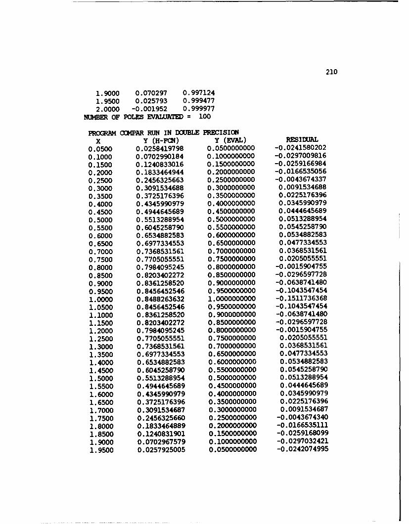
210

1.9000 0.070297 0.9971241.9500 0.025793 0.9994772.0000 -0.001952 0.999977

NUNBE OF POLES EVAIUATED = 100

PROGRM COMPAR RUN IN DOUBLE PRECISIONIX Y (H-Fa4) Y (EVAL) RESIDUAL

0.0500 0.0258419798 0.0500000000 -0.02415802020.1000 0.0702990184 0.1000000000 -0.02970098160.1500 0.1240833016 0.1500000000 -0.02591669840.2000 0.1833464944 0.2000000000 -0.01665350560.2500 0.2456325663 0.2500000000 -0.00436743370.3000 0.3091534688 0.3000000000 0.00915346880.3500 0.3725176396 0.3500000000 0.02251763960.4000 0.4345990979 0.4000000000 0.03459909790.4500 0.4944645689 0.4500000000 0.04446456890.5000 0.5513288954 0.5000000000 0.05132889540.5500 0.6045258790 0.5500000000 0.05452587900.6000 0.6534882583 0.6000000000 0.05348825830.6500 0.6977334553 0.6500000000 0.04773345530.7000 0.7368531561 0.7000000000 0.03685315610.7500 0.7705055551 0.7500000000 0.02050555510.8000 0.7984095245 0.8000000000 -0.00159047550.8500 0.8203402272 0.8500000000 -0.02965977280.9000 0.8361258520 0.9000000000 -0.06387414800.9500 0.8456452546 0.9500000000 -0.10435474541.0000 0.8488263632 1.0000000000 -0.15117363681.0500 0.8456452546 0.9500000000 -0.10435474541.1000 0.8361258520 0.9000000000 -0.06387414801.1500 0.8203402272 0.8500000000 -0.02965977281.2000 0.7984095245 0.8000000000 -0.00159047551.2500 0.7705055551 0.7500000000 0.02050555511.3000 0.7368531561 0.7000000000 0.03685315611.3500 0.6977334553 0.6500000000 0.04773345531.4000 0.6534882583 0.6000000000 0.05348825831.4500 0.6045258790 0.5500000000 0.05452587901.5000 0.5513288954 0.5000000000 0.05132889541.5500 0.4944645689 0.4500000000 0.04446456891.6000 0.4345990979 0.4000000000 0.03459909791.6500 0.3725176396 0.3500000000 0.02251763961.7000 0.3091534687 0.3000000000 0.00915346871.7500 0.2456325660 0.2500000000 -0.00436743401.8000 0.1833464889 0.2000000000 -0.01665351111.8500 0.1240831901 0.1500000000 -0.02591680991.9000 0.0702967579 0.1000000000 -0.02970324211.9500 0.0257925005 0.0500000000 -0.0242074995

211

2.0000 -0.0019520985 0.0000000000 -0.0019520985ESTIMATED SSE IS 0.0920133337ESTIMATED MSE IS 0.0023003333THE MAXIMUM ABSOLUTE DIFFERENCE BETWEEN THEH-PUNCTICN AND THE ACTUAL FUNCTIOtN IS 0.1511736368THE INTEGRATED ABSOLUTE DENSITY DIFFERENCE(AN ESTIMATE OF THE AREA BTWEE THEH-F NCTION AND THE ACTUAL DENSITY) IS 0.0752034552

EXAMPLE 4 - SUM OFTWO INDEPENDENT, IDENTICALLY

DISTRIBUTED BETA VARIATES

PROGRAM SUMVAR RUN IN DXBLE PRECISICKFOR THE SUM OF 2 INDEP7DENT H-IUNCrTIt VARIATESINPUT PARAMETERS FOR VARIABLE NUMBER 1 OF THE SIM:

M, N, P, Q = 1 0 1 1K, C = 2.0000000 1.0000000a, A = 2.00000 1.00000b, B = 0.00000 1.00000THE MOMENTS ABOUT THE ORIGIN ARE:

THE ZEROTHMOMT IS 1.0000000THE FIRST MOMENT IS 0.3333333THE SECOND CMENT IS 0.1666667THE THIRD MOMENT IS 0.1000000THE FOURTH MOMENT IS 0.0666667THE FIFTH MOMENT IS 0.0476190THE NEXT MOMENT IS 0.0357143THE NEXT MODMENT IS 0.0277778THE NEXT MOMENT IS 0.0222222THE NEXT M43ENT IS 0.0181818THE NEXT MCKENT IS 0.0151515

INPUT PARAMETERS FOR VARIABLE NUMBER 2 OF THE 4:M, N, P,Q = 1 0 1 1K, C = 2.0000000 1.0000000a, A = 2.00000 1.00000b, B = 0.00000 1.00000THE MOMENTS ABOUT THE ORIGIN ARE:

THE ZEROTH MCMENT IS 1.0000000THE FIRST M34M T IS 0.3333333THE SECOND M14MT IS 0.1666667THE THIRD MOMENT IS 0.1000000THEM FURTH MMOllET IS 0.0666667

212

THE FIFTH M4ENT IS 0.0476190THE NEXT ]MMETI IS 0.0357143THE NEXT MOMENT IS 0.0277778THE NEXT M14ENT IS 0.0222222THE NEXT MOMIT IS 0.0181818THE NEXT ]MOMENT IS 0.0151515

FOR THE RANDOM VARIABLE GIVEN AS THE S[IMOF THE ABOVE INDEPENDENT H-EUNCTIONVARIATES, THE MIMENTS ABOUT THE ORIGIN ARE:

THE ZEROTH MOMENT IS 1.0000000THE FIRST MMENT IS 0.6666667THE SECOIND MOMENT IS 0.5555556THE THIRD MET IS 0.5333333THE FOURTH MOMET IS 0.5666667THE FIFTH MIDENT IS 0.6507937THE NEXT MOMENT IS 0.7952381THE NEXT MOMENT IS 1.0222222THE NEXT MOMENT IS 1.3703704THE NEXT MET IS 1.9030303THE NEXT MCMENIT IS 2.7229437

PROGRAM HFIT RUN WITH DOUBLE PRECISIONINPUT WAS OF TYPEDTHE ZEROTH WENT WAS USED IN THE FITRESULTS OF ANALYTIC SOLUTION -NUMERATOR:

SMALLB (1) = 1.333333333333333204BIGB(1)= 1.000000000000000000

DDI(INATOR:SHALLA(1)= 5.999999999999999556BIGA(1)= 1.000000000000000000

VALUES OF K & C ARE:K-- 302.358560865130122863C= 0.500000000000000000

ESTIMATED H-FUNCTIN PARAMETERSFOR THE SMt4 OF THE INDEPENDENTH-FUNCTION VARIATES ARE:

M, N, P, Q = 1 0 1 1K, C = 302.3585609 0.5000000a, A = 6.00000 1.00000b, B = 1.33333 1.00000

THE MOMENTS ABOUT THE ORIGIN OF THISH-FUNCTION ARE:

THE ZEROTH MMENT IS 1.0000000

213

THE FIRST MOEWIT IS 0.6666667THE SECOND MOME T IS 0.5555556THE THIRD MOMENT IS 0.5349794THE FOURTH MOME T IS 0.5706447THE FIFTH MCMENT IS 0.6571060THE NEXT MNaENT IS 0.8031296THE NEXT MOMENT IS 1.0296533THE NEXT MCME T IS 1.3728711THE NEXT MOMENT IS 1.8915113THE NEXT MOMENT IS 2.6796410

DETERMINE P.D.F.(Z) AND C.D.F.(Z)FOR VALUES OF Z FROM 0.0500 TO 2.0000WITH STEP SIZE 0.0500F R THE SUM OF 1 TERMS, WHERETHE MAXIM4 NUMBER OF POLES TO BE EVAL;JATED IS 100.CRUIP PARAMETERS: NUMBER OF COMPLEX VALUES = 1001,PERCENT OF HIGHiEST Z VALUE = 1.00, AXIS POINT A 4.7785FORM FOR OVERALL PROBLEM (WHERE YJ = XJ**PJ):Z =YVARIATE X 1 IS TYPE NUMBER 4INPUT PARAMETERS ARE THETA = 302.35856, PHI = 0.50000AND PCWER = 1.00000THE P.D.F. FOR VARIATE X 1 IS GIVEN BY:

1 0 ( 6.000, 1.000)302.35856 H ( 0.50000 X):

1 1 ( 1.333, 1.000)THE P.D.F. FOR TERM 1 OF THE SUM IS GIVEN BY:

1 0302.35856 H ( 0.50000 Z), WHERE

1 1(BA(I),GBA(I)): ( 1.333, 1.000) ((CD(I),GCD(I)): ( 6.000, 1.000) (COVERGENCE TYPE= 7

D = 0.00 E 0.00 L = -4.67 R 1.0000z PDF(Z) CDF(Z)

0.0500 0.136922 0.0030180.1000 0.313676 0.0142470.1500 0.488431 0.0343430.2000 0.648272 0.0628380.2500 0.787247 0.0988210.3000 0.902663 0.1411690.3500 0.993688 0.1886800.4000 1.060648 0.2401370.4500 1.104632 0.2943610.5000 1.127231 0.350243

214

0.5500 1.130362 0.4067600.6000 1.116150 0.4629900.6500 1.086825 0.5181230.7000 1.044659 0.5714590.7500 0.991905 0.6224120.8000 0.930756 0.6705100.8500 0.863314 0.7153830.9000 0.791555 0.7567690.9500 0.717316 0.7944981.0000 0.642271 0.8284871.0500 0.567924 0.8587361.1000 0.495600 0.8853141.1500 0.426434 0.9083491.2000 0.361374 0.9280251.2500 0.301178 0.9445681.3000 0.246416 0.9582341.3500 0.197475 0.9693061.4000 0.154565 0.9780821.4500 0.117726 0.9848641.5000 0.086842 0.9899541.5500 0.061651 0.9936431.6000 0.041760 0.9962071.6500 0.026665 0.9978991.7000 0.015767 0.9989441.7500 0.008399 0.9995351.8000 0.003848 0.9998311.8500 0.001390 0.9999541.9000 0.000326 0.9999931.9500 0.000026 1.0000002.0000 -0.000001 1.000000

NUME OF POLES EVALUATED = 100

PR0PM CCHPAR RUN IN DOUBLE PRECISIONx Y (H-FCN) Y (EVAL) RESIDUAL

0.0500 0.1369215248 0.1900833333 -0.05316180850.1000 0.3136760423 0.3606666667 -0.04699062440.1500 0.4884305603 0.5122500001 -0.02381943980.2000 0.6482720923 0.6453333335 0.00293875880.2500 0.7872469795 0.7604166670 0.02683031250.3000 0.9026634638 0.8580000005 0.04466346330.3500 0.9936878985 0.9385833342 0.05510456430.4000 1.0606483104 1.0026666679 0.05798164250.4500 1.1046322658 1.0507500018 0.05388226400.5000 1.1272305972 1.0833333358 0.04389726140.5500 1.1303624979 1.1009166700 0.02944582790.6000 1.1161501217 1.1040000043 0.0121501174

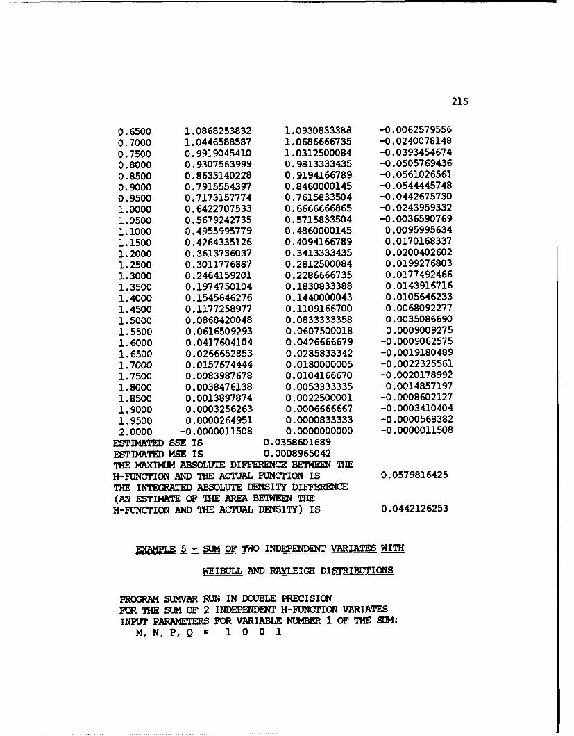
215

0.6500 1.0868253832 1.0930833388 -0.00625795560.7000 1.0446588587 1.0686666735 -0.02400781480.7500 0.9919045410 1.0312500084 -0.03934546740.8000 0.9307563999 0.9813333435 -0.05057694360.8500 0.8633140228 0.9194166789 -0.05610265610.9000 0.7915554397 0.8460000145 -0.05444457480.9500 0.7173157774 0.7615833504 -0.04426757301.0000 0.6422707533 0.6666666865 -0.02439593321.0500 0.5679242735 0.5715833504 -0.00365907691.1000 0.4955995779 0.4860000145 0.00959956341.1500 0.4264335126 0.4094166789 0.01701683371.2000 0.3613736037 0.3413333435 0.02004026021.2500 0.3011776887 0.2812500084 0.01992768031.3000 0.2464159201 0.2286666735 0.01774924661.3500 0.1974750104 0.1830833388 0.01439167161.4000 0.1545646276 0.1440000043 0.01056462331.4500 0.1177258977 0.1109166700 0.00680922771.5000 0.0868420048 0.0833333358 0.00350866901.5500 0.0616509293 0.0607500018 0.00090092751.6000 0.0417604104 0.0426666679 -0.00090625751.6500 0.0266652853 0.0285833342 -0.00191804891.7000 0.0157674444 0.0180000005 -0.00223255611.7500 0.0083987678 0.0104166670 -0.00201789921.8000 0.0038476138 0.0053333335 -0.00148571971.8500 0.0013897874 0.0022500001 -0.00086021271.9000 0.0003256263 0.0006666667 -0.00034104041.9500 0.0000264951 0.0000833333 -0.00005683822.0000 -0.0000011508 0.0000000000 -0.0000011508ESTIMATED SSE IS 0.0358601689ESTIMATED MSE IS 0.0008965042THE MAXIIMM ABSOLUTE DIFFERENCE BETWEEN THEH-FUNCTION AND THE ACTUAL FUNCTION IS 0.0579816425THE INTEGRATED ABSOLUTE DENSITY DIFFERENCE(AN ESTIMATE OF THE AREA BETWEEN THEH-FUNCTION AND THE ACI'UAL DEN2SITY) IS 0.0442126253

EXAMPLE 5 - SUM OF 'IWO INDPEDENT VARIATES WITH

WEIBULL AND RAYLEIGH DISTRIBUTIONS

PROGRAM SUMVAR RUN IN DOUBLE PRECISIONFCR THE SUM OF 2 INDEPEDET H-FUNCTION VARIATESINPUT PARAMETERS FOR VARIABLE NUMBER 1 OF THE SaM:

M, N, P,Q 1 0 0 1

216

K, C = 1.3195079 1.3195079b, B = 0.80000 0.20000THE MCMENTS ABOUT THE ORIGIN ARE:

THE ZEROTH MC)ET IS 1.0000000THE FIRST MCMET IS 0.6958418THE SECOND MCMENT IS 0.5095992THE THIRD MOMENT IS 0.3889251THE FOURTH MOMENT IS 0.3072421THE FIFTH MOMENT IS 0.2500000THE NEXT MOMENT IS 0.2087525THE NEXT MOMENT IS 0.1783597THE NEXT MKMENT IS 0.1555701THE NEXT MOMENT IS 0.1382589THE NEXT MOMENT IS 0.1250000

INPUT PARAMEMERS FOR VARIABLE NUMBER 2 OF THE SUM:M, N, P,Q = 1 0 0 1K, C = 1.7320508 1.7320508b, B = 0.50000 0.50000THE MCMENTS ABOUT THE ORIGIN ARE:

THE ZEROTH MOMENT IS 1.0000000THE FIRST MOMENT IS 0.5116634THE SECOND MOMENT IS 0.3333333THE THIRD MOMENT IS 0.2558317THE FOURTH MCM ENT IS 0.2222222THE FIFTH MOMENIT IS 0.2131931THE NEXT M14EMT IS 0.2222222THE NEXT MOMENT IS 0.2487252THE NEXT MOMENT IS 0.2962963THE NEXT MOMENT IS 0.3730879THE NEXT MOMENT IS 0.4938272

FOR THE RANDOM VARIABLE GIVEN AS THE SUMOF THE ABOVE INDEPENDENT H-FUNCTIONVARIATES, THE MOMENTS AB(XT THE ORIGIN ARE:

THE ZEROTH MOMENT IS 1.0000000THE FIRST MOMENT IS 1.2075051THE SECOND MOMENT IS 1.5550061THE THIRD MOMENT IS 2.1228284THE FOURTH MO ENT IS 3.0567312THE FIFTH MOMENT IS 4.6225066THE NEXT MOMENT IS 7.3134235THE NEXT MOMENT IS 12.0647384THE NEXT MOMENT IS 20.6900000THE NEXT MOMENT IS 36.7858797THE NEXT MOMENT IS 67.6453356

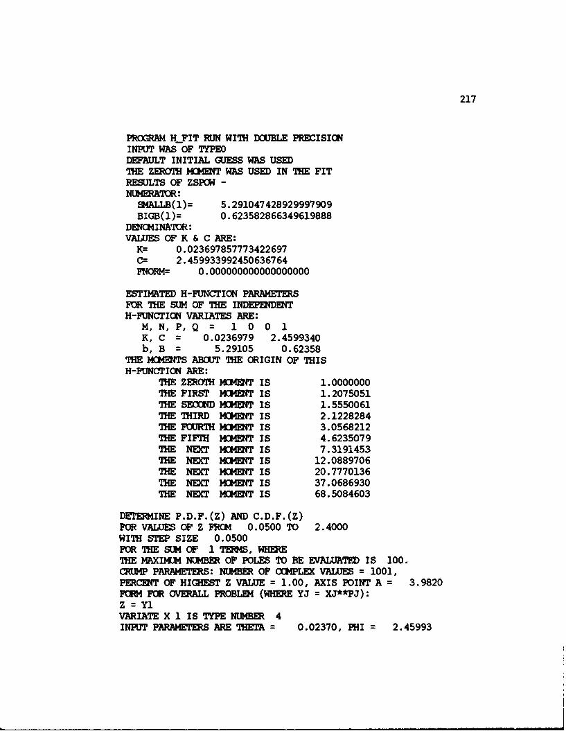
217

PROGRAM H_FIT RUN WITH DCUBLE PRECISIONINPUT WAS OF TYPEDDEFAULT INITIAL (JESS WAS USEDTHE ZEROTH MHENT WAS USED IN THE FITRESULTS OF ZSPOW -NUMERATOR:

SMALLB(1)= 5.291047428929997909BIGB(1)= 0.623582866349619888

D]NCMINATOR:VALUES OF K & C ARE:

K-- 0.023697857773422697C= 2.459933992450636764FNORM= 0.000000000000000000

ESTIMATED H-FUNCTION PARAMETERSFOR THE SLM OF THE INDEPENDNTH-FUNCTION VARIATES ARE:

M, N, P,Q = 1 0 0 1K, C = 0.0236979 2.4599340b, B = 5.29105 0.62358

THE MO4ERTS ABOUT THE ORIGIN OF THISH-FUNCTION ARE:

THE ZEROTH MCHENT IS 1.0000000THE FIRST MOMENT IS 1.2075051THE SEODM MONT IS 1.5550061THE THIRD MOMW IS 2.1228284THE FOIRTH MMET IS 3.0568212THE FIFTH MMM2T IS 4.6235079THE NEXT MOMENT IS 7.3191453THE NEXT MEXT IS 12.0889706THE NEXT MC4ENT IS 20.7770136THE NEXT MCHET IS 37.0686930THE NEXT MCa4E T IS 68.5084603

DETERMINE P.D.F.(Z) AND C.D.F.(Z)PCR VALUES OF Z FROM 0.0500 TO 2.4000WITH STEP SIZE 0.0500FOR THE SUM OF 1 TERMS, WHERETHE MAXIMUM NUMBER OF POLES TO BE EVALUATED IS 100.CRUMP PARAMETERS: NIUMBER OF CMPLEX VALUES = 1001,PERCENT OF HIGHEST Z VALUE= 1.00, AXIS POINT A = 3.9820F RM FOR OVERALL PROBLM (WHERE YJ = XJ**PJ):Z = Y1VARIATE X 1 IS TYPE NU4BER 4INPUT PARAMETERS ARE THETA= 0.02370, PHI = 2.45993

218

AND POWER = 1.00000THE P.D.F. FOR VARIATE X 1 IS GIVEN BY:

1 00.02370 H ( 2.45993 X):

0 1 ( 5.291, 0.624)THE P.D.F. FOR TERM 1 OF THE SE IS GIVi BY:

1 00.02370 H ( 2.45993 Z), WHIRE

0 1(BA(I),CBA(I)): ( 5.291, 0.624) (a)NVERGEICE TYPE = 1

D = 0.62 E = -0.62 L = 4.79 R = 1.3425z PDF(Z) CDF(Z)

0.0500 0.000000 0.0000000.1000 0.000000 0.0000000.1500 0.000007 0.0000000.2000 0.000067 0.0000010.2500 0.000388 0.0000110.3000 0.001561 0.0000540.3500 0.004860 0.0002020.4000 0.012505 0.0006120.4500 0.027742 0.0015790.5000 0.054613 0.0035800.5500 0.097399 0.0073050.6000 0.159805 0.0136480.6500 0.244059 0.0236510.7000 0.350144 0.0384190.7500 0.475360 0.0589860.8000 0.614318 0.0861850.8500 0.759413 0.1205210.9000 0.901657 0.1620790.9500 1.031744 0.2104841.0000 1.141135 0.2649081.0500 1.223000 0.3241371.1000 1.272868 0.3866731.1500 1.288939 0.4508591.2000 1.272029 0.5150161.2500 1.225228 0.5775631.3000 1.153351 0.6371201.3500 1.062279 0.6925781.4000 0.958308 0.7431331.4500 0.847563 0.7882961.5000 0.735552 0.8278691.5500 0.626854 0.8619071.6000 0.524979 0.8906691.6500 0.432336 0.914559

219

1.7000 0.350321 0.9340801.7500 0.279456 0.9497781.8000 0.219576 0.9622091.8500 0.170015 0.9719071.9000 0.129779 0.9793661.9500 0.097705 0.9850212.0000 0.072574 0.9892522.0500 0.053205 0.9923752.1000 0.038504 0.9946502.1500 0.027513 0.9962872.2000 0.019386 0.9974482.2500 0.013441 0.9982622.3000 0.009088 0.9988192.3500 0.005791 0.9991882.4000 0.002836 0.999396

NUMBR OF POLES EVA~LUATED 94

APPEIDIX B

GRAPHICAL DEPICTIONS OF SLIMS OF SELECTED INDEPEIDENT

UNIFORM, POWER FUNCTION, AND BETA VARIATES

Listed below are graphical depictions of the examples in

Section 5.1.1 of analytic convolutions performed to find the

exact distribution of the sum of selected independent randan

variables. The exact distributions of sum of two independent

variates with certain uniform, power function, and beta

distributions were found using the convolution integral. These

graphs may provide some insight to the sum of independent

variates with a restricted range. These sums produce a

distribution with two functional form over distinct ranges of

the variable and do not have continuous derivatives of all

orders at x=1.

The two leftmost graphs in each row show the densities of

each random variable in the sum, f XlJX and fx (x). The

rightmost graph in each row shows the density of Y=XI+X ,

y(y), when X, and X2 are independent. Each series of graphs

is also referenced to the corresponding equation number frm

Section 5.1.1.

220

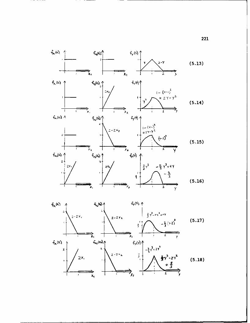
221

(5.15)

2Y 2

a+

.3

222

(y-

z4 (5.20)

_____ _____ _ 1* ____

(5.20)

223

z -, ( I(5.22)

-rs

yX Y4 Y '

I YZ44Y

IL I y_( .4

224

-qy +, (5.25)

AS

2-

l y €2 (5.26)

L '-- -,I i

-*22Y ,4Y

(5.26)

1I 2 1

BIBLIOGRAPHY

Abramowitz, M. and I. A. Stegun (Editors), Handbook ofMathematical Functions with Formulas, Graphs, and MathematicalTables, National Bureau of Standards, U.S. Department ofCommerce, AMS 55, ninth printing, (1970).

Andrews, L.C., Special Functions for Engineers and AppliedMathematicians, Macmillan Publishing Co., New York, (1985).

Artin, E., The Gamma Function, Holt, Rinehart and Winston, NewYork, (1964).

Barnes, J. W., C. D. Zinn, and B. S. Eldred, "A Methodology forObtaining the Probability Density Function of the Present Worthof Probabilistic Cash Flow Profiles," AIIE Transactions,10:226-236, (1978).

Bodenschatz, C. D., and J. W. Barnes, "On the Sum ofIndependent, Non-Identically Distributed Erlang RandomVariables," Graduate Program in Operations Research TechnicalReport Series, The University of Texas at Austin, ORP91-07,Manuscript submitted for publication, in second review, (1991).

Bodenschatz, C. D., J. W. Barnes, and I. D. Cook, Jr., "H-Function Representations of Power Functions and Beta-TypeFunctions," Unpublished working paper, The University of Texasat Austin, (1991).

Bodenschatz, C. D., J. W. Barnes, W. T. Guy, Jr., and I. D.Cook, Jr., "Convergence Conditions for the H-Function,"Unpublished working paper, The University of Texas at Austin,(1992).

Bodenschatz, C. D., and R. A. Boedigheimer, An Application ofthe H-Function to Curve-Fitting and Density Estimation,Master's Thesis, Air Force Institute of Technology, (December1983).

225

226

Bodenschatz, C. D., R. A. Boedigheimer, and I. D. Cook, Jr.,"New and Generalized H-Function Distributions," AnericanJournal of Mathemtical and Manaaeient Sciences, 10:185-191,(1990).

Boedigheiner, R. A., C. D. Bodenschatz, and I. D. Cook, Jr.,"An Application of the H-Function to Curve-Fitting and DensityEstination," Graduate Program in Operations Research TechnicalReport Series, The University of Texas at Austin, ORP91-09,Manuscript submitted for publication, in second review, (1984).

Carter, B. D., On the Probability Distribution of RationalFunctions of Independent H-Function Variates, Ph.D.Dissertation, The University of Arkansas, (May 1972).

Carter, B. D. and M. D. Springer, "The Distribution ofProducts, Quotients, and Powers of Independent H-FunctionVariates," SIAM Journal of Applied Mathematics, 33:542-558,(1977).

Churchill, R. V., Operational Mathematics, McGraw-Hill BookCompany, New York, (1972).

Cook, I. D., Jr., The H-Function and Probability DensityFunctions of Certain Algebraic Combinations of IndependentRandom Variables with H-Function Probability Distributions,Ph.D. Dissertation, The University of Texas at Austin, (May1981).

Cook, I. D., Jr. and J. W. Barnes, "Evaluation of the H-Function Integral and of Probability Distributions of Functionsof Independent Randm Variables," American Journal ofMathematical and Management Sciences, 1:293-339, (1981).

Cook, I. D., Jr. and J. W. Barnes, "The Cumulative DistributionFunction and Distribution Constant of an H-runctionDistribution," Graduate Program in Operations ResearchTechnical Report Series, The University of Texas at Austin,ORP91-02, Manuscript submitted for publication, (1991).

Cook, I. D., Jr. and J. W. Barnes, "New H-FunctionRepresentations for Various Functions Based on Their MellinTransformations," Manuscript submitted for publication, (1991).

227

Cramfir, H. Random Variables and Probability Distributions,Cambridge University Press, London, (1970).

Crunip, K. S., "Numerical Inversion of Laplace Transforms Usinga Fourier Series Approximation," Journal of the Association forCumputing Machinery, 23:89-96, (1976).

Davies, B., Integral Transforms and Their Applications,Springer-Verlag, Inc., New York, (1978).

DeGroot, M. H., Probability and Statistics, Addison-WesleyPublishing, Co., Reading, Mass., (1975).

Dixon, A. L. and W. L. Ferrar, "A Class of DiscontinuousIntegrals," The Ouarterly Journal of Mathematics, OxfordSeries, 7:81-96, (1936).

Doetsch, G., Guide to the Applications of the Laplace and Z-Transforms, Van Nostrand Reinhold Co., London, (1971).

Elderton, W. P. and N. L. Johnson, Systems of Frequency Curves,Cambridge University Press, London, (1969).

Eldred, B. S., A Methodology for Obtaining the ProbabilityDensity Function of the Present Worth of Probabilistic CashFlow Profiles, Ph.D. Dissertation, The University of Texas atAustin, (May 1979).

Eldred, B. S., J. W. Barnes, and I. D. Cook, Jr., "Applicationof Convergence Conditions to Evaluation of General Mellin-Barnes Integrals," Unpublished working paper, The University ofTexas at Austin, (1979).

Erd~lyi, A., Asymptotic Expansions, Dover Publications, Inc.,New York, (1956).

Erd~lyi, A. (Editor), Higher Transcendental Functions, Vol. 1,Bateman Manuscript Project, McGraw-Hill Book Co., Inc., NewYork, (1953).

Erd6lyi, A. (Editor), Higher Transcendental Functions, Vol. 2,Bateman Manuscript Project, McGraw-Hill Book Co., Inc., NewYork, (1953).

228

Erd~lyi, A., Operational Calculus and Generalized Functions,Holt, Rinehart and Winston, Inc., New York, (1962).

Erd6lyi, A. (Editor), Tables of Integral Transforms, Vol. 1,Batefmn Manuscript Project, McGraw-Hill Book Co., Inc., NewYork, (1954).

Eshbach, 0. W. and M. Souders (Editors), Handbook ofEngineering Fundamentals, John Wiley and Sons, New York,(1975).

Feller, W., An Introduction to Probability Theory and ItsApplications Vol. 1, John Wiley and Sons, New York, (1968).

Fox, C., "The G and H Functions as Symretric Fourier Kernels,"Transactions of the American Mathematical Society, 98:395-429,(1961).

Gnedenko, B. V., The Theory of Probability, Chelsea PublishingCo., New York, (1962).

Hardy, G. H., Divergent Series, Oxford University Press,London, (1949).

Hastings, N. A. J., and J. B. Peacock, StatisticalDistributions, Butterworth & Co. (Publishers) Ltd., London,(1975).

Hiebert, K. L., A Carparison of Software Which Solves Systemsof Nonlinear Equations, Sandia National Laboratories, KirtlandAir Force Base, New Mexico, (1980).

Hill, T. W., Jr., On Determininq a Distribution Function KnownOnly by Its Manents and/or Moment Generating Function, Ph.D.Dissertation, Arizona State University, (1969).

Hirschmnn, I. I., Infinite Series, Holt, Rinehart, andWinston, Inc., New York, (1962).

Jacobs, H. W., Curve Fitting Probability Density Functionsusing the H-Function, Ph.D. Dissertation, The University ofTexas at Austin, (May 1986).

229

Jacobs, H. W., J. W. Barnes, and I. D. Cook, Jr., "Applicationsof the H-Function Distribution in Classifying and FittingClassical Probability Distributions," American Journal ofMathematical and Management Sciences, 7:131-147, (1987).

Johnson, N. L. and S. Kotz, Continuous Univariate Distributions-i, Houghton Mifflin Co., Boston, (1970).

Kellogg, S. D., Algebraic Functions of H-Functions withSpecific Dependency Structures, Ph.D. Dissertation, TheUniversity of Texas at Austin, (May 1984).

Kellogg, S. D., and J. W. Barnes, "The Bivariate H-FunctionDistribution," Mathematics and Coputers in Simulation, 31:91-111, (1989).

Kellogg, S. D., and J. W. Barnes, "The Distribution ofProducts, Quotients, and Powers of Two Dependent H-FunctionVariates," Mathematics and Conuters in Simulation, 29:209-221,(1987).

Kendall, M. G. and A. Stuart, The Advanced Theory ofStatistics, Vol. 1: Distribution Theory, Charles Griffin & Co.,Ltd., London, (1969).

Kleinrock, L., Oueueing System. Volume 1: Theory, John Wileyand Sons, New York, (1975).

Knopp, K., Infinite Sequences and Series, Dover Publications,Inc., New York, (1956).

LePage, W. R., Ccuplex Variables and the Laplace Transform forEngineers, McGraw-Hill Book Co., New York, (1961).

Lindgren, B. W., Statistical Theory, Maaillan Publishing Co.,Inc., New York, (1976).

Lindgren, B. W. and G. W. McElrath, Introduction to Probabilityand Statistics, The Maaillan Co., New York, (1959).

Lukacs, E., Developments in Characteristic Function Theory,Charles Griffin & Ccnqany Ltd., London (1983).

230

Mathai, A. M. and R. K. Saxena, "Applications of SpecialFunctions in the Characterization of ProbabilityDistributions," South African Statistical Journal, 3:27-34,(1969).

Mathai, A. M. and R. K. Saxena, The H-Function withApplications in Statistics and Other Disciplines, John Wiley &Sons, New York, (1978).

Mood, A. M., F. A. Graybill, and D. C. Boes, Introduction tothe Theory of Statistics, McGraw-Hill Inc., New York, (1974).

Moore, C. N., Sumible Series and Convergence Factors, AmericanMathematical Society, New York, (1938).

Neuts, M., Probability, Allyn and Bacon, Inc., Boston, (1973).

Oberhettinger, F., Fourier Transforms of Distributions andTheir Inverses, Academic Press, New York, (1973).

Petrov, V. V., Sums of Independent Random Variables, Springer-Verlag, Berlin, (1975).

Prasad, R. D., "Probability Distributions of AlgebraicFunctions of Independent Random Variables," SIAM Journal ofApplied Mathemtics, 18:614-626, (1970).

Prudnikov, A. P., Y. A. Brychkov, and 0. I. Marichev, Integralsand Series, Vol. 3, More Special Functions, Gordon and BreachScience Publishers, OPA, Amsterdam, (1990).

Smith, M. G., Laplace Transform Theory, D. Van Nostrand Co.Ltd., London, (1966).

Springer, M. D., The Algebra of Random Variables, John Wiley &Sons, New York, (1979).

Springer, M. D., "Evaluation of the H-Function InversionIntegral for Real Variables using Jordan's Lein and Residues,"SIAM Journal of Applied Mathenatics, 47:416-424, (1987).

Springer, M. D. and W. E. Thapson, "The Distribution ofProducts of Independent Randan Variables," SIAM Journal ofApplied Mathematics, 14:511-526, (1966).

231

Srivastava, H. M., K. C. Gupta, and S. P. Goyal, The H-Functions of one and Two Variables, with Applications, SouthAsian Publishers Pvt. Ltd., New Delhi, (1982).

Stacy, E. W., "A Generalization of the Gamma Function," Annalsof Mathematical Statistics, 33:1187-1192, (1962).

Stacy, E. W., and G. A. Mihram, "Parameter Estiration for aGeneralized Gamma Distribution," Technauetrics, 7:349-358,(1965).

Steutel, F. W., Preservation of Infinite Divisibility underMixing and Related Topics, Matheratical Centre Tracts 33,Mathematisch Centrum, Arsterdam, (1970).

Thcrpson, W. T., Laplace Transformation, Prentice-Hall, Inc.,Englewood Cliffs, NJ, (1960).

Whittaker, E. T. and G. N. Watson, A Course of Modern Analysis,Cambridge University Press, London, (1927).

Widder, D. V., The Laplace Transform, Princeton UniversityPress, (1941).

VITA

Captain Carl Dinsnore Bodenschatz was born in Chanpaign-Urbana,

Illinois on June 16, 1957, the son of Mary Joan Dinsmore

Bodenschatz and Carl Alvin Bodenschatz. In 1975, he graduated

fram Henpfield Area High School in Greensburg, Pennsylvania.

After working as a Quality Control Lab Technician at

Kennametal, Inc. in Latrobe, Pennsylvania for 14 months, he

entered West Virginia University in Morgantown, West Virginia.

In college, he majored in Mathematics with a minor in

Statistics. In May 1980, he received the degree of Bachelor of

Arts (magna cum laude) fram West Virginia University. Upon

graduation, he received a commission in the U.S. Air Force

through the four-year ROTC program. In Deceber 1983, he

received the degree of Master of Science in Operations Research

fram the Air Force Institute of Technology, Wright-Patterson

Air Force Base, Ohio. His other Air Force assigrinents have

included working as a Training System Analyst and Operational

Test and Evaluation Analyst at Eglin Air Force Base, Florida

and as an Instructor in the Department of Mathematical Sciences

at the U.S. Air Force Academy, Colorado. He is the principal

author of "New and Generalized H-function Distributions",

published in 1990 by the American Journal of Mathematical and

Management Sciences. He entered the Graduate School of The

University of Texas in August 1989. He married Deborah Murdock

of Greensburg, Pennsylvania on May 31, 1980. They have three

children, Luke Murdock born in 1981 and twins John Oakwood and

Paul Oveson born in 1984.

Permanent Address: 110 Sherwood Drive

Greensburg, Pennsylvania 15601

This dissertation was typed by the author.