Sequences and Series: A Sourcebook Pete L. Clark

Sequences and Series: A Sourcebook

Pete L. Clark

c©Pete L. Clark, 2012.Thanks most of all to N.J. Diepeveen for his help in proving an �exercise� in anearly copy of these notes. Thanks to Didier Piau for an important correction.

Thanks to Jorge Nicolás Caro Montoya for pointing out typos.

Contents

Introduction 5

Chapter 0. Foundations 71. Prerequisites 72. Number Systems 73. Sequences 84. Binary Operations 115. Binary Relations 126. Ordered Sets 137. Upper and Lower Bounds 168. Intervals and Convergence 179. Fields 1810. Ordered Fields 2111. Archimedean Ordered Fields 23

Chapter 1. Real Sequences 251. Least Upper Bounds 252. Monotone Sequences 263. The Bolzano-Weierstrass Theorem 294. The Extended Real Numbers 315. Partial Limits 316. The Limit Supremum and Limit In�mum 327. Cauchy Sequences 348. Sequentially Complete Non-Archimedean Ordered Fields 369. The Stolz-Cesaro Theorem 38

Chapter 2. Real Series 391. Introduction 392. Basic Operations on Series 443. Series With Non-Negative Terms I: Comparison 484. Series With Non-Negative Terms II: Condensation and Integration 545. Series With Non-Negative Terms III: Ratios and Roots 646. Series With Non-Negative Terms IV: Still More Convergence Tests 677. Absolute Convergence 708. Non-Absolute Convergence 749. Rearrangements and Unordered Summation 8110. Power Series I: Power Series as Series 92

Chapter 3. Sequences and Series of Functions 1011. Pointwise and Uniform Convergence 101

3

4 CONTENTS

2. Power Series II: Power Series as (Wonderful) Functions 1103. Taylor Polynomials and Taylor Theorems 1114. Taylor Series 1165. The Binomial Series 1206. The Weierstrass Approximation Theorem 123

Bibliography 127

Introduction

This is a text concerned with the theory of in�nite sequences and series, largely atan intermediate undergraduate level. The proximate cause of the text is the Math3100 course that I taught at UGA in Spring 2011, which (as usual) motivated meto type up my own notes.

The current text is admittedly a bit strange, and it is not necessarily intendedfor use in an undergraduate course. Rather the purpose upon conception was tobe supplementary to what appears in more standard texts. In the 19th century,the theory of in�nite series was the crown jewel of mathematics, and most of theleading mathematicians contributed to it in some way. In our day this is no longerthe case. On the contrary, for a while now the �theory of in�nite series� has beensynonymous with certain chapters in undergraduate real analysis. One can evenput a �ner point on it: after the introduction of Rudin's breakthrough text [R],what an American student learns about in�nite series is some (or better, all) ofChapters 3 and 7 of [R]. Let me be clear: I �nd these chapters (especially thelatter) to be the high points of what must be the most in�uential and successfulof all American mathematical textbooks. And yet there is � must be � more toin�nite series than what �ts in these 75 pages, and there must be other valid �even novel � takes on the material. In fact the most recent generation of Americantexts has followed up on the latter point, if not the former. It is now recognizedthat relatively few undergraduate math majors are prepared for a presentation likeRudin's, and the most successful contemporary texts are more student friendly. Ido not in any way object to this trend, but the current text does not participate init: though I know a positive number of undergraduate students who have read andlearned from (various drafts of) this text, it is intended more for the instructorsof such courses than the students than the students themselves. Most of all it isintended for me, and in places it is openly experimenal: I have tried out certainthings in order to determine which aspects of them (if any) may be suitable toinclude in actual lectures to actual undergraduates.

The desire to be di�erent at any price is most clearly evident in Chapter 0. Thisis an approach to the foundations of the subject as might be done by Little NickyBourbaki. The conceit here is that the theory of in�nite series arises from thecon�uence of multiple structures: (i) sequences in a set R; (ii) a total ordering onR, which provides a notion of convergence, and which satis�es any of several com-pleteness properties (iii) the compatible structure of a �eld on R. Saying things thisway makes one want to analyze the setup: how much can be said when some butnot all of these structures are present? One may well say that this kind of generalnonsense is antithetical to the contentful concreteness of �real real analysis,� and

5

6 INTRODUCTION

I have several colleagues who would say at least this much. I would say that Iam participating in the recent trend of �real analysis in reverse� which � thoughmotivated by any number of things which have little to do with the substance ofreal analysis, nevertheless has a way of cutting to the core of �what is really goingon� in undergraduate analysis, with some nice payo�s both at the research leveland (more importantly, to me) pedagogically.

Most �real real analysts� would agree that just about the worst thing to spendtime on in any undergraduate analysis course is a formal construction of the realnumbers. What is less acknowledged, but I think must be true, is that the reasonfor this is the full success of the structural approach to the real numbers: they arecharacterized as being the unique complete ordered �eld (here �complete� can beconstrued in several di�erent ways and the statement remains true). Thus there isat least some promise beginning the theory of sequences and series with a structuralapproach.

Here is a �nal remark about Chapter 0: it is almost dispensable. Most of theconcepts which are given in obnoxious generality in Chapter 0 are repeated in thecase of R in Chapter 1. I would advise anyone using this text in an Americanundergraduate course to start with Chapter 1 and dip backwards into Chapter 0 ifneeded.

CHAPTER 0

Foundations

1. Prerequisites

These notes are for a student who has had some prior exposure to proofs, basicmathematical structures and mathematical abstraction. At UGA these concepts aretaught in Math 3200. We will draw more strongly on having a certain minimumcomfort level with such things than on any speci�c prior knowledge, but for instancethe student should be familiar with the following terms:

set, subset, proper subset, power set, cardinality of a �nite set, relation, equiv-alence relation, partition, function, injection, surjection, bijection.

2. Number Systems

We begin by reminding the reader about basic number systems. One should viewthis as being little more than �xing notation: sophisticated readers will know thatthere is some mathematical content involved in giving complete de�nitions of thesestructures. It is by no means our goal to do so here.

We de�neZ+ = {1, 2, 3, . . . , n, . . .},

the set of positive integers. We de�ne

N = {0, 1, 2, 3, . . . , n, . . .},the set of natural numbers. Note that the two sets N and Z+ di�er precisely inthat 0 is a member of the natural numbers and is not a member of the positive in-tegers. There are some (very minor) mathematical reasons behind this distinction,but in practice it functions mostly as a convention. Moreover it is not a universallyheld one, and when you read or hear others using the terms �positive integers� or�natural numbers,� you will need to �gure out from the context � or ask � whether0 is meant to be included. (And it is annoying, because the answer is not veryimportant, but a misunderstanding could still cause some trouble.)

We de�neZ = {. . . ,−3,−2,−1, 0, 1, 2, 3, . . .},

the set of integers.

We de�ne

Q ={ab| a, b ∈ Z, b 6= 0

},

the set of rational numbers.

7

8 0. FOUNDATIONS

We de�ne R to be the set of real numbers . This is a point where a formal de�ni-tion is challenging enough to be unhelpful for a beginning student, but roughly thereal numbers are the mathematical structure which make precise the idea of �pointson the number line�. A non-negative real number can be thought of as a distancebetween two points (in the Euclidean plane or Euclidean space), which need not bea rational quantity. One can represent any real number by its decimal expansion:

a0.a1a2 . . . an . . .

Here a0 is an integer and

a1, a2, . . . ∈ {0, 1, 2, 3, 4, 5, 6, 7, 8, 9}

are decimal digits. To make real sense out of this de�nition requires the theoryof sequences and series! Later on in this chapter we will give not a de�nition of Rbut a perfectly e�ective and useful operational description of them: they form acomplete ordered �eld. (You are not supposed to know what these terms mean yet.)

We de�ne

C = {x+ yi | x, y ∈ R, i2 = −1}to be the set of complex numbers.

Each of these number systems is a proper subset of the next: we have

Z+ ( N ( Z ( Q ( R ( C.

3. Sequences

Let X be a set. A sequence in X is a function x : Z+ → X. Thus, as for anyfunction, for each element n ∈ Z+ we must assign exactly one element x(n) ∈ X.This has the e�ect of giving us an in�nite ordered list of elements of X:

x(1), x(2), x(3), . . . , x(n), . . . .

We say that e.g. x(3) is the 3rd term of the sequence and in general that x(n) isthe nth term of the sequence.

Example 0.1. For a set X, we denote the set of sequences in X by XZ+

. (Thisis a case of the notation Y X for the set of functions from a set X to a set Y .)a) Suppose X = ∅. Then a sequence in X is a function from the nonempty set Z+

to the empty set ∅. There are no such functions, so there are no sequences in X.b) Suppose #X = 1, i.e., X = {•} has a single element. A sequence in X is afunction from the set Z+ to the one-point set {•}. There is exactly one function:we must have x(n) = • for all n ∈ Z+.c) Things become considerably more interesting when X has at least two elements.Suppose that #X = 2, and to �x notation, take X = {0, 1}. A sequence Z+ → {0, 1}is called an (in�nite) binary sequence. This is an extremely basic, important anduseful mathematical structure. We can represent every real number between 0 and1 by an in�nite binary sequence, for instance. (Unfortunately the representation isnot always unique, an annoyance that we do not need to deal with at the moment.)More to the point, the collection of all in�nite binary sequences {f : Z+ → {0, 1}}is naturally in bijection with the power set 2Z

+

, i.e., the set of all subsets of Z+.

3. SEQUENCES 9

Namely, let S ⊂ Z+ be a subset. To S we associate the binary sequence s(S): forn ∈ Z+, we put s(S) = 1 if n ∈ S and s(S) = 0 if n /∈ S. This gives us a map

s : 2Z+

→ {0, 1}Z+

.

To see that s is a bijection we write down the inverse function

t : {0, 1}Z+

→ 2Z+

.

Namely, to any binary sequence x : Z+ → {0, 1} we associate the subset t(x) ={n ∈ Z+ | x(n) = 1}. I leave it to you to check that for any subset S ⊂ Z+ we havet(s(S)) = S and that for any binary sequence x : Z+ → {0, 1} we have s(t(x)) = x.d) We will be most interested in the case of sequences in R. This is a very largeset. (Those who are familiar with cardinalities of in�nite sets may wish to show

that the cardinality of the set RZ+

of all rael sequences has the same cardinality asthat of the power set 2R of all real numbers. Those who are not: no worries.)

The �theory of in�nite sequences� really means the theory of sequences in R, C orclosely related things (e.g. RN ). There is very little �theory of sequences in anarbitrary set X.� Very little but not none: we now give some.

To a sequence x : Z+ → X we can associate the set

x(Z+) = {x(n) ∈ X | n ∈ Z+}

of all terms of the sequence. This is just the image of the corresponding function.Notice that knowing the sequence itself is more information than knowing its image:consider in particular the case of binary sequences: X = {0, 1}. There is exactlyone binary sequence with image 0, namely

0, 0, 0, . . . , 0, . . .

There is exactly one binary sequence with image 1, namely

1, 1, 1, . . . , 1, . . .

All others have image {0, 1}: there are (uncountably) in�nitely many of them.

Let f : X → Y be a function. Given a sequence x : Z+ → X in X, we canpush it forward to a sequence f∗(x) in X by

f∗(x) : n 7→ f(x(n)).

In other words, f∗(x) is simply the composite function f ◦ x : Z+ → Y .

Example 0.2. Let x : Z+ → Z+ by x(n) = n2. Thus x is a sequence in Z.a) Using the inclusion map f : Z ↪→ R we can view x as a sequence of real numbers:f∗(x)(n) = n2 ∈ R.b) Let f : Z+ → {0, 1} by f(n) = 0 if n is even and f(n) = 1 if n is odd. (That is:we map an integer to its class modulo 2.) We push forward the integer sequence

1, 4, 9, 16, 25, 36, 49, . . .

to get the binary sequence

1, 0, 1, 0, 1, 0, 1, 0 . . . .

(We have such a nice pattern here because n2 is even i� n is even.)

10 0. FOUNDATIONS

Exercise 0.1. Let f : X → Y be a map of nonempty sets. Consider theassociated map

f∗ : XZ+

→ Y Z+

, x 7→ (n 7→ f(x(n))).

a) Show: f∗ is injective i� f is injective.b) Show: f∗ is surjecive i� f is surjective.c) Deduce: f∗ is bijective i� f is bijective.

However, if we have a sequence y : Z+ → Y in a set Y and a function f : X → Y ,it does not make sense to �pull back� y to a sequence in X: the functions don'tcompose correctly. However, if we have a sequence x : Z+ → X and a functiong : Z+ → Z+, we get a new sequence by precomposing with g:

g∗(x) = x ◦ g : Z+ → X, n 7→ x(g(n)).

In full generality this is a rather strange operation. We single out two special caseswhich will become signi�cant later.

Suppose g : Z+ → Z+ is strictly increasing: if n1 < n2 then g(x1) < g(x2).Then the process of passing from x to g∗x is called passing to a subsequence.

Example 0.3. The function g : Z+ → Z+ by n 7→ n2 is strictly increasing, andthis process carries a sequence

x(1), x(2), x(3), . . . , x(n), . . .

tox(1), x(4), x(9), . . . , x(n), . . . .

Exercise 0.2. Let I be the set of all strictly increasing functions g : Z+ → Z+.We de�ne a function

Φ : I → 2Z+

from I to the power set of Z+ by mapping each function to its image:

Φ : g 7→ g(Z+) ⊂ Z+.

Show: Φ is an injection with image the set of all in�nite subsets of Z+.

The previous exercise reconciles our de�nition of a subsequence with another (per-haps more natural and useful) way of thinking about them: namely, passage to asubsequence means choosing an in�nite set S of positive integers and only keepingthe terms xn of the sequence with n ∈ S.

The other case in which precomposing a sequence with a function g : Z+ → Z+ isa reasonable thing to do in real life is when the function g;Z+ → Z+ is a bijection.Then we may view g∗x as a rearrangement of x.

Example 0.4. Let g : Z+ → Z+ be the map which for all n ∈ Z+ interchangesthe 2n− 1 and 2n: thus

g(1) = 2, g(2) = 1, g(3) = 4, g(4) = 3, g(5) = 6, g(6) = 5, . . . .

Then precomposing with g carries the sequence

x(1), x(2), x(3), x(4), x(5), x(6) . . .

to the sequencex(2), x(1), x(4), x(3), x(6), x(5) . . . .

4. BINARY OPERATIONS 11

Remark: We wished to spend a little time with the notation x(n) to drive the pointhome that a sequence is a function. However no one actually uses this notation forsequences: rather, everyone writes n 7→ xn....and so will we.

4. Binary Operations

Let S be a set. A binary operation on S is simply a function from S × Sto S. Rather than using multivariate function notation � i.e., (x, y) 7→ f(x, y) � itis common to �x a symbol, say ∗, and denote the binary operation by (x, y) 7→ x∗y.

A binary operation is commutative if for all x, y ∈ S, x ∗ y = y ∗ x.

A binary operation is associative if for all x, y, z ∈ S, (x ∗ y) ∗ z = x ∗ (y ∗ z).

Example 0.5. Let S = Q be the set of rational numbers. Then addition (+),subtraction (−) and multiplication (·) are all binary operations on S. Note thatdivision is not a binary operation on Q because it is not everywhere de�ned: thesymbol a÷ b has no meaning if b = 0.

As is well known, + and · are both commutative and associative whereas it iseasy to see that − is neither commutative nor associative: e.g.

3− 2 = 1 6= 2− 3,

(1− 0)− 1 = 0 6= 2 = 1− (0− 1).

Perhaps the most familiar binary operation which is associative but not commuta-tive is matrix multiplication. Precisely, �x an integer n ≥ 2 and let S = Mn(Q) bethe set of n× n square matrices with rational entries.

Exercise 0.3. Give an example of a binary operation which is commutativebut not associative. In fact, give at least two examples, in which the �rst one hasthe set S �nite and as small as possible (e.g. is it possible to take S to have twoelements?). Give a second example in which the operation is as �natural� as youcan think of: i.e., if you told it to someone else, they would recognize that operationand not accuse you of having made it up on the spot.

Let ∗ be a binary operation on a set S. We say that an element e ∈ S is an identityelement (for ∗) if for all x ∈ S,

e ∗ x = x ∗ e = x.

Remark: If ∗ is commutative (as will be the case in the examples of interest to ushere) then of course we have e ∗ x = x ∗ e for all x ∈ S, so in the de�nition of anidentity it would be enough to require x ∗ e = x for all x ∈ S.

Proposition 0.6. A binary operation ∗ on a set S has at most one identityelement.

Proof. Suppose e and e′ are identity elements for ∗. The dirty trick is to playthem o� each other: consider e ∗ e′. Since e is an identity, we must have e ∗ e′ = e′,and similarly, since e′ is an identity, we must have e ∗ e′ = e, and thus e = e′. �

Example 0.7. For the operation + on Q, there is an identity: 0. For theoperation · on Q, there is an identity: 1. For matrix multiplication on Mn(Q),there is an identity: the n× n identity matrix In.

12 0. FOUNDATIONS

Example 0.8. The addition operation + on Q restricts to a binary operationon Z+ (that is, the sum of any two positive integers is again a positive integer).Since by our convention 0 /∈ Z+, it is not clear that (Z+,+) has an identity element,and indeed a moment's thought shows that it does not.

Suppose (S, ∗) is a binary operation on a set which possesses an identity element e.For an element x ∈ S, an element x′ ∈ S is said to be inverse to x (with respectto ∗) if x ∗ x′ = x′ ∗ x = e.

Proposition 0.9. Let (S, ∗) be an associative binary oepration with an identityelement e. Let x ∈ S be any element. Then x has at most one inverse.

Proof. It's the same trick: suppose x′ and x′′ are both inverses of x withrespect to ∗. We have x ∗ x′ = e, and now we apply x′′ �on the left� to both sides:

x′′ = x′′ ∗ e = x′′ ∗ (x ∗ x′) = (x′′ ∗ x) ∗ x′ = e ∗ x′ = x′. �

Example 0.10. For the operation + on Q, every element x has an inverse,namely −x = (−1) · x. For the operation · on Q, every nonzero element has aninverse, but 0 does not have a multiplicative inverse: for any x ∈ Q, 0 · x = 0 6= 1.(Later we will prove that this sort of thing holds in any �eld.)

5. Binary Relations

Let S be a set. Recall that a binary relation on S is given by a subset R of theCartesian product S2 = S × S. Restated in equivalent but less formal terms, foreach ordered pair (x, y) ∈ S×, either (x, y) lies in the relation R � in which case wesometimes write xRy � or (x, y) does not lie in the relation R.

For any binary relation R on S and any x ∈ S, we de�ne

[x]R = {y ∈ S | (x, y) ∈ R},

R[x] = {y ∈ S | (y, x) ∈ R}.In words, [x]R is the set of elements of S which are related to R �on the right�, and

R[x] is the set of elements of S which are related to R �on the left�.

Example 0.11. Let S be the set of people in the world, and let R be the par-enthood relation, i.e., (x, y) ∈ R i� x is the parent of y. Then [x]R is the set of x'schildren and R[x] is the set of x's parents.

Here are some important properties that a relation R ⊂ S2 may satisfy.

(R) Re�exivity: for all x ∈ S, (x, x) ∈ R.(S) Symmetry: for all x, y ∈ S, (x, y) ∈ R =⇒ (y, x) ∈ R.(AS) Antisymmetry: for all x, y ∈ S, if (x, y) ∈ R and (y, x) ∈ R then x = y.(Tr) Transitivity: for all x, y, z ∈ S, if (x, y) ∈ R and (y, z) ∈ R then (x, z) ∈ R.(To) Totality: for all x, y ∈ S, either (x, y) ∈ R or (y, x) ∈ R (or both).

Exercise 0.4. Let R be a binary relation on a set S.a) Show: R is re�exive i� for all x ∈ S, x ∈ [x]R i� for all x ∈ S, x ∈ R[x].b) Show: R is symmetric i� for all x ∈ S, [x]R = R[x]. In this case we put

[x] = [x]R =R[x].

6. ORDERED SETS 13

c) Show: R is antisymmetric i� for all x, y ∈ S, x ∈ R[y], y ∈ [x]R implies x = y.d) Show R is transitive i� for all x, y, z ∈ S, x ∈ R[y] and y ∈ R[z] implies x ∈R[z].e) Show that R is total i� for all x ∈ R, either x ∈ R[y] or x ∈ [y]R.

An equivalence relation is a relation which is re�exive, symmetric and transitive.

If R is an equivalence relation on x, we call

[x] =R[x] = [x]R

the equivalence class of R.Let R be an equivalence relation on S, suppose that for x, y, z ∈ S we have

z ∈ [x]∩[y]. Then transitivity gives (x, y) ∈ R. Moreover if x′ ∈ [x] then (x, x′) ∈ R,(x, y) ∈ R and hence (x′, y) ∈ R, i.e., x′ ∈ [y]. Thus [x] ⊂ [y]. Arguing similarlywith the roles of x and y interchanged gives [y] ⊂ [x] and thus [x] = [y]. That is,any two distinct equivalence classes are disjoint. Since by re�exivity, for all x ∈ S,x ∈ [x], it follows that the distinct equivalence classes give a partition of S.

The converse is also true: if X =⋃i∈I Xi is a partition of X � i.e., for all i ∈ I,

Xi is nonempty, for all i 6= j, Xi ∩Xj = ∅ and every element of X lies in some Xi,then there is an induced equivalence relation R by de�ning (x, y) ∈ R i� x, y lie inthe same element of the partition.

6. Ordered Sets

A partial ordering on S is a relation R which is re�exive, anti-symmetric andtransitive. We then commonly write x ≤ y for (x, y) ∈ R. We also refer to the pair(S,≤) as a partially ordered set. A totally ordered set is a partially orderedset (S,≤) satisfying totality: for all x, y ∈ S, either x ≤ y or y ≤ x.

Example 0.12. (The Key Example) The real numbers R under the standard≤ is a totally ordered set.

It will be useful to borrow some auxiliary notation from the above case. Namely,for a partially ordered set (S,≤) and x, y ∈ S, we write y ≥ x to mean x ≤ y. Wealso write x < y to mean x ≤ y and x 6= y, and �nally y > x to mean x < y.

Exercise 0.5.For a partially ordered set (S,≤), we may view < as a relation on S.a) Show that the relation < satis�es:(i) anti-re�exivitiy: for no x ∈ S do we have x < x.(ii) strict anti-symmetry: for no x, y ∈ S do we have x < y and y < x.(iii) transitivity.b) Conversely, we say a relation < on a set S is a strict partial ordering if it isanti-re�exive, strictly anti-symmetric and transitive. Given a strict partial ordering< on S, de�ne a new relation ≤ by x ≤ y i� x < y or x = y. Show: ≤ is a partialordering on S.c) Check that the processes of passing from a partial ordering to a strict partialordering and of passing from a strict partial ordering to a partial ordering aremutually inverse. (The upshot is that we can work with < or ≤ as the basic relation;nothing is lost either way.)

14 0. FOUNDATIONS

Exercise 0.6. Let X be a set, and let R be the equality relation on X: that is,(x, y) ∈ R ⇐⇒ x = y.a) Show: R is an equivalence relation on X.b) Show: R is a partial ordering on X.c) Show: conversely, if R′ is a relation on X which is both an equivalence relationand a partial ordering, then R′ = R.

We call a partially ordered set (X,≤) totally disordered if ≤ is the equalityrelation, i.e., x ≤ y ⇐⇒ x = y. Thus every set can be made into a totallydisordered partially ordered set in a unique way.

Example 0.13. For a set X, let S = 2X be the power set of X (the set of allsubsets of X). The containment relation on subsets of X is a partial orderingon S: that is, for subsets A,B of X, we put A ≤ B i� A ⊂ B. Note that assoon as X has at least two distinct elements x1, x2, there are subsets A and B suchthat neither is contained in the other, namely A = {x1}, B = {x2}. Thus we haveneither A ≤ B nor B ≤ A.

In general, two elements x, y in a partially ordered set are comparable if x ≤ y ory ≤ x; otherwise we say they are incomparable. A total ordering is thus a partialordering in which any two elements are comparable.

A bottom element b in a partially ordered set (S,≤) is an element of S suchthat b ≤ x for all x ∈ S. Similarly a top element t in (S,≤) is an element of Ssuch that x ≤ t for all x ∈ S.

Exercise 0.7. a) Show: a partially ordered set has at most one bottom elementand at most one top element.b) Show: every power set (2X ,≤) admits a bottom element and a top element. Whatare they?c) Show: (Z,≤) has neither a bottom element nor a top element.d) Suppose that in a partially ordered set (S,≤) we have a bottom element m, a topelement M and moreover m = M . What can be said about S?e) Show: a �nite, nonempty totally ordered set has bottom and top elements.

We now have a pair of closely related concepts: an element m in a partially orderedset (S,≤) is minimal if there does not exist x ∈ S with x < m. An element M ina partially ordered set (S,≤) is maximal if there does not exist ∈ S with M < y.

Proposition 0.14. a) In any partially ordered set, a bottom element is minimaland a top element is maximal.b) In a totally ordered set, a minimal element is a bottom element and a maximalelement is a top element.c) A partially ordered set can have a minimal element which is not a bottom elementand a maximal which is not a top element.

Proof. a) If b is a bottom element, then for all x 6= b we have b < x, so wecannot also have x < b: b is minimal. The argument for top elements is similar andleft to the reader.b) Let m be a minimal element in a totally ordered set, and let x 6= m. We cannothave x < m and we are totally ordered, so we must have m < x: m is a bottomelement. The argument maximal elements is similar and left to the reader.

6. ORDERED SETS 15

c) Let X be a set with more than one element, and endow it with the equalityrelation. Then for no x, y ∈ X do we have x < y, so every element of X is bothminimal and maximal, and X has neither bottom nor top elements. �

Comment on terminology: I am sorry to tell you that some people say �max-imum� instead of �top element� and �minimum� instead of �bottom element� of apartially ordered set. In a totally ordered set, Proposition 0.14b) ensures this is�ne, and we will usually refer to the top and bottom elements of a totally orderedset in this way. However, in a partially ordered set that is not totally ordered, thisterminology is most unfortunate: e.g. Proposition 0.14c) would read: �A partiallyordered set can have a minimal element which is not a minimum and a maximalelement which is not a maximum.� Thus changing an adjective to a noun changesthe mathematical meaning!

Now let {xn}∞n=1 be a sequence in the partially ordered set (S,≤). We say thatthe sequence is increasing (respectively, strictly increasing) if for all m ≤ n,xm ≤ xn (resp. xm < xn). Similarly, we say that the sequence is decreasing (respectively, strictly decreasing if for all m ≤ n, xm ≥ xn (resp. xm > xn).

A partially ordered set (S,≤) is well-founded if there is no strictly decreasingsequence {xn}∞n=1 in S. A well-ordered set is a well-founded totally ordered set.

Let R be a relation on S, and let T ⊂ S. We de�ne the restriction of R toT as the set of all elements (x, y) ∈ R ∩ (T × T ). We denote this by R|T . F

Exercise 0.8. Let R be a binary relation on S, and let T be a subset of S.a) Show: if R is an equivalence relation, then R|T is an equivalence relation on T .b) Show that if R is a partial ordering, then R|T is a partial ordering on T .c) Show that if R is a total ordering, then R|T is a total ordering on T .d) Show that if R is a well-founded partial ordering, then R|T is a well-foundedpartial ordering on T .

Proposition 0.15. For a totally ordered (S,≤), the following are equivalent:(i) S is well-founded: it admits no in�nite strictly decreasing sequence.(ii) For every nonempty subset T of S, the restricted totally ordered set (T,≤) hasa bottom element.

Proof. (i) =⇒ (ii): We go by contrapositive: suppose that there is anonempty subset T ⊂ S without a minimum element. From this it follows imme-diately that there is a strictly decreasing sequence in T : indeed, by nonemptiness,choose x1 ∈ T . Since x1 is not the minimum in the totally ordered set T , theremust exist x2 ∈ T with x2 < x1. Since x2 is not the minimum in the totally orderedset T , there must exist x3 in T with x3 < x2. Continuing in this way we build astrictly decreasing sequence in T and thus T is not well-founded. It follows that Sitself is not well-founded, e.g. by Exercise 0.4d), but let's spell it out: an in�nitestrictly decreasing sequence in the subset T of S is, in particular, an in�nite strictlydecreasing sequence in S!(ii) =⇒ (i): Again we go by contrapositive: suppose that {xn} is a strictly de-creasing sequence in S. Then let T be the underlying set of the sequence: it is anonempty set without a minimum element! �

16 0. FOUNDATIONS

Example 0.16. (Key Example): For any integer N , the set Z≥N of integersgreater than or equal to N is well-ordered: there are no strictly decreasing in�nitesequences of integers all of whose terms are at least N .1

Exercise 0.9. Let (X,≤) be a totally ordered set. De�ne a subset Y of X tobe inductive if for each x ∈ X, if Ix = {y ∈ X | y < x} ⊆ Y , then x ∈ Y .a) Show that X is well-ordered i� the only inductive subset of X is X itself.b) Explain why the result of part a) is a generalization of the principle of mathe-matical induction.

Let x, y be elements of a totally ordered set X. We say that y covers x if x < yand there does not exist z ∈ X with x < z < y.

Example 0.17. In X = Z, y covers X i� y = x + 1. In X = Q, no elementcovers any other element.

A totally ordered set X is right discrete if for all x ∈ X, either x is the topelement of X or there exists y in X such that y covers x. A totally ordered setX is left discrete if for all x ∈ X, either x is the bottom element of X or thereexists z in X such that x covers z. A totally ordered set is discrete if it is bothleft discrete and right discrete.

Exercise 0.10. a) Show that (Z,≤) is discrete.b) Show that any subset of a discrete totally ordered set is also discrete.

7. Upper and Lower Bounds

Let (S,≤) be a partially ordered set, and let Y ⊂ S. We say M ∈ S is an upperbound for Y if y ≤ M for all y ∈ Y . We say m ∈ S is a lower bound for Y ifm ≤ y for all y ∈ Y .

Notice that if M is an upper bound for Y and M ′ > M then also M ′ is an upperbound for Y . So in general a subset will have many upper bounds. If the set ofall upper bounds of Y has a bottom element, we call that the supremum or leastupper bound of Y and denote it by sup(Y ). Similarly, if m is a lower bound forY and m′ < m then also m′ is a lower bound for Y . If the set of all lower boundsof Y has a top element, we call tha the in�mum or greatest lower bound of Yand denote it by inf(Y ). Since a partially ordered set can have at most one bottomelement and at most one top element, sup(Y ) is unique if it exists and so is inf(Y ).

Exercise 0.11. Let (S,≤) be a partially ordered set.a) Show: sup(∅) exists i� X has a bottom element b, in which case sup(∅) = b.b) Show: inf(∅) exists i� X has a top element t, in which case inf(∅) = t.

A lattice is a partially ordered set (S,≤) in which every two element subset {a, b}has an in�mum and a supremum. In this case it is traditional to write

a ∨ b = sup({a, b}), a ∧ b = inf({a, b}).

1As usual in these notes, we treat structures like N, Z and Q as being known to the reader.This is not to say that we expect the reader to have witnessed a formal construction of them.Such formalities would be necessary to prove that the natural numbers are well-ordered, and oneday the reader may like to see it, but such considerations take us backwards into the foundationsof mathematics in terms of formal set theory, rather than forwards as we want to go.

8. INTERVALS AND CONVERGENCE 17

A totally ordered set is certainly a lattice, since we have

a ∨ b = max(a, b), a ∧ b = min(a, b).

A complete lattice is a partially ordered set (S,≤) in which every subset Y(including Y = ∅) has a supremum and an in�mum. A Dedekind completelattice is a partially ordered set (S,≤) in which every nonempty subset which isbounded above admits a supremum.

Example 0.18. A �nite nonempty totally ordered set is a complete lattice.

Example 0.19. Let X be a set. Then the partially ordered set (2X ,⊂) isDedekind complete. If Y ⊂ 2X , then Y is a family of subsets of X, and we have

sup(Y ) =⋃A∈Y

A, inf(Y ) =⋂A∈Y

A.

Exercise 0.12. a) Let (X,≤) be a partially ordered set in which every subsethas a supremum. Show: X is a complete lattice.b) Let (X,≤) be a partially ordered set in which every nonempty bounded abovesubset has a supremum. Show: X is a Dedekind complete lattice.c) Let (X,≤) be a partially ordered set in which every subset has an in�mum. Show:X is a complete lattice.d) Let (X,≤) be a partially ordered set in which every nonempty bounded belowsubset has an in�mum. Show: X is a Dedekind complete lattice.e) Let (X,≤) be a Dedekind complete lattice. Show: X is a complete lattice i� ithas a top element and a bottom element.

8. Intervals and Convergence

Let (S,≤) be a totally ordered set, and let x < y be elements of S.

We de�ne intervals(x, y) = {z ∈ S | x < z < y},[x, y) = {z ∈ S | x ≤ z < y},(x, y] = {z ∈ S | x < z ≤ y},[x, y] = {z ∈ S | x ≤ z ≤ y.

These are straightforward generalizations of the notion of intervals on the real line.The intervals (x, y) are called open. We also de�ne

(−∞, y) = {z ∈ S | z < y},(−∞, y] = {z ∈ S | z ≤ y},(x,∞) = {z ∈ S | x < z},[x,∞) = {z ∈ S | z ≤ z}.

The intervals (−∞, y) and [x,∞) are also called open. Finally,

(−∞,∞) = S

is also called open.

There are some subtleties in these de�nitions. Depending upon the ordered setS, some intervals which �do not look open� may in fact be open. For instance,suppose that S = Z with its usual ordering. Then for any m ≤ n ∈ Z, the interval

18 0. FOUNDATIONS

[m,n] does not look open, but it is also equal to (m − 1, n + 1), and so it is. Foranother example, let S = [0, 1] the unit interval in R with the restricted ordering.Then by de�nition (−∞, 12 ) is an open interval, which by de�nition is the same set

as [0, 12 ). The following exercise nails down this phenomenon in the general case.

Exercise 0.13. Let (S,≤) be a totally ordered set.a) If S has a minimum element m, then for any x > m, the interval [m,x) is equalto (−∞, x) and is thus open.b) If S has a maximum element M , then for any x < M , the interval (x,M ] isequal to (x,∞) and is thus open.

Let xn : Z+ → X be a sequence with values in a totally ordered set (X,≤). Wesay that the sequence converges to x ∈ X if for every open interval I containingx, there exists N ∈ Z+ such that for all n ≥ N , xn ∈ I.

9. Fields

9.1. The Field Axioms.

A �eld is a set F endowed with two binary operations + and · satisfying thefollowing �eld axioms:(F1) + is commutative, associative, has an identity element � called 0 � and everyelement of F has an inverse with respect to +.(F2) · is commutative, associative, has an identity element � called 1 � and everyx 6= 0 has an inverse with respect to ·.(F3) (Distributive Law) For all x, y, z ∈ F , (x+ y) · z = (x · z) + (y · z).(F4) 0 6= 1.

Thus any �eld has at least two elements, 0 and 1.

Example 0.20. The rational numbers Q, the real numbers R and the complexnumbers C are all �elds under the familiar binary operations of + and ·. Wetreat these as known facts: that is, it is not our ambition here to construct any ofthese �elds from simpler mathematical structures (although this can be done andthe reader may want to see it someday).

It is common to abbreviate x · y to just xy, and we shall feel free to do so here.

Remark: The de�nition of a �eld consists of three structures: the set F , the binaryoperation + : F × F → F and the binary operation · : F × F → F . Thus weshould speak of �the �eld (F,+, ·)�. But this is tedious and is in fact not done inpractice: one speaks e.g. of �the �eld Q�, and the speci�c binary operations + and ·are supposed to be understood. This sort of practice in mathematics is so commonthat it has its own name: abuse of notation.

Example 0.21. There is a �eld F with precisely two elements 0 and 1. Indeed,the axioms completely determine the �addition and multiplication tables� of such anF : we must have 0 + 0 = 0, 0 + 1 = 1, 0 · 0 = 0, 0 · 1 = 0, 1 · 1 = 1. Keeping inmind the commutativity of + and ·, the only missing entry from these �tables� is1 + 1: what is that? Well, there are only two possibilities: 1 + 1 = 0 or 1 + 1 = 1.But the second possibility is not tenable: letting z be the additive inverse of 1 andadding it both sides of 1 + 1 = 1 cancels the 1 and gives 1 = 0, in violation of (F4).

9. FIELDS 19

Thus 1 + 1 = 0 is the only possibility. Converesely, it is easy to check that theseaddition and multiplication tables do indeed make F = {0, 1} into a �eld. This isin fact quite a famous and important example of a �eld, denoted either F2 or Z/2Zand called the binary �eld or the �eld of integers modulo 2. It is importantin set theory, logic and computer science, due for instance to the interpretation of+ as �OR� and · as �AND�.

Example 0.22. Let N ≥ 2 be an integer. Let Z/NZ be the set {0, 1, . . . , N−1},and consider the following binary operations on Z/NZ: for x, y ∈ Z/NZ, x + y(resp. xy) is de�ned by �rst taking the usual sum x+ y ∈ Z (resp. product xy ∈ Z)and then taking the remainder upon division by N . This generalizes the previousexample, which took N = 2.

It is not di�cult to show that the set Z/NZ endowed with these two binaryoperations satis�es axioms (F1), (F3) and (F4). Moreover it satis�es most of (F2):the multiplication is commutative, associative, has an identity element � the integer1 � however it need not be the case that every nonzero element has a multiplicativeinverse. For example, if N = 4, then the element 2 has no multiplicative inverse:2 · 1 = 2 · 3 = 2 and 2 · 0 = 2 · 2 = 0. More generally, if N is not a prime number,then there are integers 1 < a, b < N such that ab = N , and then then the elementa has no multiplicative inverse: if xa = 1, then

0 = x(0) = x(ab) = (xa)b = 1(b) = b.

It turns out that when N = p is a prime number, then every nonzero element has amultiplicative inverse, so Z/pZ is a �eld, often denoted Fp. This uses a nontrivialresult from number theory, Euclid's Lemma, and as we do not need �nite �eldsfor anything in these notes, we will leave things there.

9.2. Some simple consequences of the �eld axioms.

There are many, many di�erent �elds. Nevertheless the �eld axioms are rich enoughto imply certain consequences for all �elds.

Proposition 0.23. Let F be any �eld. For all x ∈ F , we have 0 · x = 0.

Proof. For all x ∈ F , 0 ·x = (0 + 0) ·x = (0 ·x) + (0 ·x). Let y be the additiveinverse of 0 · x. Adding y to both sides has the e�ect of �cancelling� the 0 · x terms:

0 = y + (0 · x) = y + ((0 · x) + (0 · x))

= (y + (0 · x)) + (0 · x) = 0 + (0 · x) = 0 · x. �

Proposition 0.24. Let (F,+, ·) be a set with two binary operations satisfyingaxioms (F1), (F2) and (F3) but not (F4): that is, we assume the �rst three axiomsand also that 1 = 0. Then F = {0} = {1} consists of a single element.

Proof. Let x be any element of F . Then

x = 1 · x = 0 · x = 0. �

Proposition 0.23 is a very simple, and familiar, instance of a relation between theadditive structure and the multiplicative structure of a �eld. We want to furtherexplore such relations and establish that certain familiar arithmetic properties holdin an arbitrary �eld.

To help out in this regard, we de�ne the element −1 of a �eld F to be the

20 0. FOUNDATIONS

additive inverse, i.e., the unique element of F such that 1 + (−1) = 0. (Note thatalthough −1 is denoted di�erently from 1, it need not actually be a distinct element:indeed in the binary �eld F2 we have 1 + 1 = 0 and thus −1 = 1.)

Proposition 0.25. Let F be a �eld and let −1 be the additive inverse of 1.Then for any element x ∈ F , (−1) · x is the additive inverse of x.

Proof.

x+ ((−1) · x) = 1 · x+ (−1) · x = (1 + (−1)) · x = 0 · x = 0. �

In light of Proposition 0.25 we create an abbreviated notation: for any x ∈ F , weabbreviate (−1) · x to −x. Thus −x is the additive inverse of x.

Proposition 0.26. For any x ∈ F , we have −(−x) = x.

Proof. We prove this in two ways. First, from the de�nition of additiveinverses, suppose y is the additive inverse of x and z is the additive inverse of y.Then, what we are trying to show is that z = x. But indeed x + y = 0 and sinceadditive inverses are unique, this means x is the additive inverse of y.

A second proof comes from identifying −x with (−1) · x: for this it will su�ceto show that (−1) · (−1) = 1. But

(−1) · (−1)− 1 = (−1) · (−1) + (1) · (−1) = (−1 + 1) · (−1) = 0 · (−1) = 0.

Adding one to both sides gives the desired result. �

Exercise 0.14. Apply Proposition 0.26 to show that for all x, y in a �eld F :a) (−x)(y) = x(−y) = −(xy).b) (−x)(−y) = xy.

For a nonzero x ∈ F our axioms give us a (necessarily unique) multiplicative inverse,which we denote � as usual � by x−1.

Proposition 0.27. For all x ∈ F \ {0}, we have (x−1)−1 = x.

Exercise 0.15. Prove Proposition 0.27.

Proposition 0.28. For x, y ∈ F , we have xy = 0 ⇐⇒ (x = 0) or (y = 0).

Proof. If x = 0, then as we have seen xy = 0 · y = 0. Similarly if y = 0,of course. Conversely, suppose xy = 0 and x 6= 0. Multiplying by x−1 givesy = x−10 = 0. �

Let F be a �eld, x ∈ F , and let n be any positive integer. Then � despite the factthat we are not assuming that our �eld F contains a copy of the ordinary integersZ � we can make sense out of n · x: this is the element x+ . . .+ x (n times).

Exercise 0.16. Let x be an element of a �eld F .a) Give a reasonable de�nition of 0 · x, where 0 is the integer 0.b) Give a reasonable de�nition of n · x, where n is a negative integer.

Thus we can, in a reasonable sense, multiply any element of a �eld by any positiveinteger (in fact, by Exercise 0.16, by any integer). We should however beware notto carry over any false expectations about this operation. For instance, if F is thebinary �eld F2, then we have 2 · 0 = 0 + 0 = 0 and 2 · 1 = 1 + 1 = 0: that is, forall x ∈ F2, 2x = 0. It follows from this for all x ∈ F2, 4x = 6x = . . . = 0. Thisexample should serve to motivate the following de�nition.

10. ORDERED FIELDS 21

A �eld F has �nite characteristic if there exists a positive integer n such thatfor all x ∈ F , nx = 0. If this is the case, the characteristic of F is the leastpositive integer n such that nx = 0 for all x ∈ F . A �eld which does not have �nitecharacteristic is said to have characteristic zero.2

Exercise 0.17. Show that the characteristic of a �eld is either 0 or a primenumber. (Hint: suppose for instance that 6x = 0 for all x ∈ F . In particular(2 · 1)(3 · 1) = 6 · 1 = 0. It follows that either 2 · 1 = 0 or 3 · 1 = 0.

Example 0.29. a) The binary �eld F2 has characteristic 2. More generally,for any prime number p, the integers modulo p form a �eld which has characteristicp. (These examples are perhaps misleading: for every prime number p, there are�elds of characteristic p which are �nite but contain more than p elements as wellas �elds of characteristic p which are in�nite. However, as we shall soon see, aslong as we are studying calculus / sequences and series / real analysis, we will notmeet �elds of positive characteristic.)b) The �elds Q,R,C have characteristic zero.

Proposition 0.30. Let F be a �eld of characteristic 0. Then F contains therational numbers Q as a sub�eld.

Proof. Since F has characteristic zero, for all n ∈ Z+, n·1 6= 0 in F . We claimthat this implies that in fact for all pairs m 6= n of distinct integers, m · 1 6= n · 1 aselements of F . Indeed, we may assume that m > n (otherwise interchange m andn) and thus m · 1−n · 1 = (m−n) · 1 6= 0. Thus the assignment n 7→ n · 1 gives us acopy of the ordinary integers Z inside our �eld F . We may thus simply write n forn ·1. Having done so, notice that for all n ∈ Z+, 0 6= n ∈ F , so 1

n ∈ F , and then for

any m ∈ Z, m 1n = m

n ∈ F . Thus F contains a copy of Q in a canonical way, i.e., viaa construction which works the same way for any �eld of characteristic zero. �

10. Ordered Fields

An ordered �eld (F,+, ·, <) is a set F equipped with the structure (+, ·) of a �eldand also with a total ordering <, satisfying the following compatbility conditions:

(OF1) For all x1, x2, y1, y2 ∈ F , x1 < x2 and y1 < y2 implies x1 + y1 < x2 + y2.(OF2) For all x, y ∈ F , x > 0 and y > 0 implies xy > 0.

The rational numbers Q and the real numbers R are familiar examples of ordered�elds. In fact the real numbers are a special kind of ordered �eld, the uniqueordered �eld satisfying any one of a number of fundamental properties which arecritical in the study of calculus and analysis. One of the main goals of this sectionis to understand these special properties of R and their interrelationships.

Proposition 0.31. For elements x, y in an ordered �eld F , if x < y, then−y < −x.

2Perhaps you were expecting �in�nite characteristic�. This would indeed be reasonable. Butthe terminology is traditional and well-established, and we would not be doing you a favor bychanging it here.

22 0. FOUNDATIONS

Proof. We rule out the other two possibilities: if −y = −x, then multiplyingby −1 gives x = y, a contradiction. If −x < −y, then adding this to x < y using(OF1) gives 0 < 0, a contradiction. �

Proposition 0.32. Let x, y be elements of an ordered �eld F .a) If x > 0 and y < 0 then xy < 0.b) If x < 0 and y < 0 then xy > 0.

Proof. a) By Proposition 0.31, y < 0 implies −y > 0 and thus x(−y) =(−xy) > 0. Applying 0.31 again, we get xy < 0.b) If x < 0 and y < 0, then −x > 0 and −y > 0 so xy = (−x)(−y) > 0. �

Proposition 0.33. Let x1, x2, y1, y2 be elements of an ordered �eld F .a) (OF1′) If x1 < x2 and y1 ≤ y2, then x1 + y1 < x2 + y2.b) (OF1′′) If x1 ≤ x2 and y1 ≤ y2, then x1 + y1 ≤ x2 + y2.

Proof. a) If y1 < y2, then this is precisely (OF1), so we may assume thaty1 = y2. We cannot have x1 + y1 = x2 + y2 for then adding −y1 = −y2 toboth sides gives x1 = x2, contradiction. Similarly, if x2 + y2 < x1 + y1, thenby Proposition 0.31) we have −y2 < −y1 and adding these two inequalities givesx2 < x1, a contradiction.b) The case where both inequalities are strict is (OF1). The case where exactly oneinequality is strict follows from part a). The case where we have equality both timesis trivial:if x1 = x2 and y1 = y2, then x1 + y1 = x2 + y2, so x1 + y1 ≤ x2 + y2. �

Remark: What we have shown is that given any �eld (F,+, ·) with a total ordering<, the axiom (OF1) implies (OF1′) and also (OF1′′). In fact (OF1′) implies (OF1)and (OF1′′) and that (OF1′′) implies (OF1)and (OF1′), so all three are equivalent.

Proposition 0.34. Let x, y be elements of an ordered �eld F .(OF2′) If x ≥ 0 and y ≥ 0 then xy ≥ 0.


Proposition 0.35. Let F be an ordered �eld and x a nonzero element of F .Then exactly one of the following holds:(i) x > 0.(ii) −x > 0.

Proof. First we show that (i) and (ii) cannot both hold. Indeed, if so, thenusing (OF1) to add the inequalities gives 0 > 0, a contradiction. (Or apply Proposi-tion 0.31: x > 0 implies −x < 0.) Next suppose neither holds: since x 6= 0 and thus−x 6= 0, we get 0 < x and 0 < −x. Adding these gives 0 < 0, a contradiction. �

Proposition 0.36. Let 0 < x < y in an ordered �eld F . Then 0 < 1y <

1x .

Proof. First observe that for any z > 0 in F , 1z > 0. Indeed, it is certainly

not zero, and if it were negative then 1 = z · 1z would be negative, by Proposition

0.32. Moreover, for x 6= y, we have 1x −

1y = (y−x) · (xy)−1. Since x < y, y−x > 0;

since x, y > 0, xy > 0 and thus (xy)−1, so 1x −

1y > 0: equivalently, 1

y <1x . �

Proposition 0.37. Let F be an ordered �eld.a) We have 1 > 0 and hence −1 < 0. b) For any x ∈ F , x2 ≥ 0.c) For any x1, . . . , xn ∈ F \ {0}, x21 + . . .+ x2n > 0.

11. ARCHIMEDEAN ORDERED FIELDS 23

Proof. a) By de�nition of a �eld, 1 6= 0, hence by Proposition 0.35 we haveeither 1 > 0 or −1 > 0. In the former case we're done, and in the latter case (OF2)gives 1 = (−1)(−1) > 0. that −1 < 0 follows from 0.31.b) If x ≥ 0, then x2 ≥ 0. Otherwise x < 0, so by Proposition 0.31, −x > 0 andthus x2 = (−x)(−x) > 0.c) This follows easily from part b) and is left as an exercise for the reader. �

Proposition 0.37 can be used to show that certains �eld cannot be ordered, i.e.,cannot be endowed with a total ordering satisfying (OF1) and (OF2). First of allthe �eld C of complex numbers cannot be ordered, because C contains an elementi such that i2 = −1, whereas by Proposition 0.37b) the square of any element inan ordered �eld is non-negative and by Proposition 0.37a) −1 is negative.

The binary �eld F2 of two elements cannot be ordered: because 0 = 1 + 1 =12 + 12 contradicts Proposition 0.37c). Similarly, the �eld Fp = Z/pZ of integersmodulo p cannot be ordered, since 0 = 1 + 1 + . . . + 1 = 12 + . . . + 12 (each sumhaving p terms). This generalizes as follows.

Corollary 0.38. An ordered �eld F must have characteristic 0.

Proof. Seeking a contradiction, suppose there is n ∈ Z+ such that n · x = 0for all x ∈ F . Then 12 + . . .+ 12 = 0, contradicting Proposition 0.37c). �

Combining Proposition 0.30 and Corollary 0.38, we see that every ordered �eldcontains a copy of the rational numbers Q.

11. Archimedean Ordered Fields

Recall that every ordered �eld (F,+, ·, <) has contained inside it a copy of therational numbers Q with the usual ordering. An ordered �eld F is Archimedeanif the subset Q is not bounded above and non-Archimedean otherwise.

Example 0.39. The ordered �eld Q is Archimedean. From our intuitive under-standing of R � e.g., by considerations involving the decimal expansion � it is clearthat R is an Archimedean �eld. (Later we will assert a stronger axiom satis�ed byR from which the Archimedean property follows.)

Non-archimedean ordered �elds do exist. Indeed, in a sense we will not try to makeprecise here, �most� ordered �elds are non-Archimedean.

Suppose F is a non-Archimedean ordered �eld, and let M be an upper boundfor Q. Then one says thatM is in�nitely large. Dually, if m is a positive elementof F such that m < 1

n for all n ∈ Z+, one says that m is in�nitely small.

Exercise 0.19. Let F be an ordered �eld, and M an element of F .a) Show that M is in�nitely large i� 1

M is in�nitely small.b) Conclude that F is Archimedean i� it does not have in�nitely large elements i�it does not have in�nitely small elements.

CHAPTER 1

Real Sequences

1. Least Upper Bounds

Proposition 1.1. Let F be an Archimedean ordered �eld, {an} a sequence inF , and L ∈ F . Then an → L i� for all m ∈ Z+ there exists N ∈ Z+ such that forall n ≥ N , |an − L| < 1

m .

Proof. Let ε > 0. By the Archimedean property, there exists m > 1ε ; by

Proposition 0.32 this implies 0 < 1m < ε. Therefore if N is as in the statement of

the proposition, for all n ≥ N ,

|an − L| <1

m< ε.

�

Exercise 1.1. Show that for an ordered �eld F the following are equivalent:(i) limn→∞ n =∞.(ii) F is Archimedean.

Proposition 1.2. For an ordered �eld F , the following are equivalent:(i) Q is dense in F : for every a < b ∈ F , there exists c ∈ Q with a < c < b.(ii) The ordering on F is Archimedean.

Proof. (i) =⇒ (ii): we show the contrapositive. Suppose the ordering on Fis non-Archimedean, and let M be an in�nitely large element. Take a = M andb = M + 1: there is no rational number in between them.(ii) =⇒ (i): We will show that for a, b ∈ F with 0 < a < b, there exists x ∈ Qwith a < x < b: the other two cases are a < 0 < b � which reduces immediately tothis case � and a < b < 0, which is handled very similarly.

Because of the nonexistence of in�nitesimal elements, there exist x1, x2 ∈ Qwith 0 < x1 < a and 0 < x2 < b − a. Thus 0 < x1 + x2 < b. Therefore the setS = {n ∈ Z+ | x1 + nx2 < b} is nonempty. By the Archimedean property S is�nite, so let N be the largest element of S. Thus x1 +Nx2 < b. Moreover we musthave a < x1 +Nx2, for if x1 +Nx2 ≤ a, then x1 + (N + 1)x2 = (x1 +Nx2) + x2 <a+ (b− a) = b, contradicting the de�nition of N . �

Let (X,≤) be an ordered set. Earlier we said that X satis�es the least upperbound axiom (LUB) if every nonempty subset S ⊂ F which is bounded abovehas a least upper bound, or supremum. Similarly, X satis�es the greatest lowerbound axiom (GLB) if every nonempty subset S ⊂ F which is bounded belowhas a greatest lower bound, or in�mum. We also showed the following basic result.

Proposition 1.3. An ordered set (X,≤) satis�es the least upper bound axiomif and only if it satis�es the greatest lower bound axiom.

25

26 1. REAL SEQUENCES

The reader may �nd all of this business about (LUB)/(GLB) in ordered �elds quiteabstract. And so it is. But our study of the foundations of real analysis takesa great leap forward when we innocently inquire which ordered �elds (F,+, ·, <)satisfy the least upper bound axiom. Indeed, we have the following assertion.

Fact 1. The real numbers R satsify (LUB): every nonempty set of real numberswhich is bounded above has a least upper bound.

Note that we said �fact� rather than �theorem�. The point is that stating thisresult as a theorem cannot, strictly speaking, be meaningful until we give a precisede�nition of the real numbers R as an ordered �eld. This will come later, butfwhat is remarkable is that we can actually go about our business without needingto know a precise de�nition (or construction) of R.

(It is not my intention to be unduly mysterious, so let me say now � for whateverit is worth � that the reason for this is that there is, in the strongest reasonablesense, exactly one Dedekind complete ordered �eld. Thus, whatever we can sayabout any such �eld is really being said about R.)

2. Monotone Sequences

A sequence {xn} with values in an ordered set (X,≤) is increasing if for all n ∈ Z+,xn ≤ xn+1. It is strictly increasing if for all n ∈ Z+, xn < xn+1. It is decreasingif for all n ∈ Z+, xn ≥ xn+1. It is strictly decreasing if for all n ∈ Z+, xn < xn+1.A sequence is monotone if it is either increasing or decreasing.

Example 1.4. A constant sequence xn = C is both increasing and decreasing.Conversely, a sequence which is both increasing and decreasing must be constant.

Example 1.5. The sequence xn = n2 is strictly increasing. Indeed, for alln ∈ Z+, xn+1 − xn = (n + 1)2 − n2 = 2n + 1 > 0. The sequence F xn = −n2 isstrictly decreasing: for all n ∈ Z+, xn+1 − xn = −(n+ 1)2 + n2 = −(2n+ 1) < 0.

Exercise 1.2. Let {xn} be an increasing (resp. strictly increasing) sequencein an ordered �eld. Show: {−xn} is decreasing (resp. strictly decreasing).

We claim that an increasing sequence is the discrete analogue of an increasingfunction in calculus. Recall that a function f : R → R is increasing if for allx1 < x2, f(x1) ≤ f(x2), is strictly increasing if for all x1 < x2, f(x1) < f(x2),and similarly for decreasing and strictly decreasing functions. Looking carefully,we notice that this does not line up preicsely with the de�nition of increasing. Butwe can resolve the situation happily.

Proposition 1.6. Let {xn} be a sequence with values in an ordered �eld. Then{xn} is increasing if and only if: for all m,n ∈ Z+, if m ≤ n then xm ≤ xn.

Proof. Suppose {xn} is increasing. Let m ∈ Z+. Then for all k ∈ Z+ we have

xm+k − xm = (xm+k − xm+k−1) + (xm+k−1 − xm+k−2) + . . .+ (xm+1 − xm).

Since {xn} is increasing, each term on the right is non-negative, so xm+k − xm isnon-negative. Taking n = m + k this gives xm ≤ xn for all n > m (and the casen = m is trivial).

The converse is immediate: if we suppose that for all m ≤ n ∈ Z+ we havexm ≤ xn, then taking n = m+ 1 shows that {xn} is increasing. �

2. MONOTONE SEQUENCES 27

Exercise 1.3. Show that Proposition 1.6 holds verbatim for sequences in anyordered set. (The point here is not to make any use of the �eld operations.) Sug-gestion: let S be the set of positive integers k such that for all m ∈ Z+, we havexm ≤ xm+k. Use induction to show S = Z+.

Exercise 1.4. Let f : R→ R be a di�erentiable function.a) Recall from calculus (or, if it is more to your taste, prove using the Mean ValueTheorem) that the following are equivalent:(i) For all x, y ∈ R, if x ≤ y then f(x) ≤ f(y).(ii) For all x ∈ R we have f ′(x) ≥ 0.b) I claim that Proposition 1.6 is the discrete analogue of part a). Do you see why?

Example 1.7. Let us show that the sequence { lognn }∞n=3 is strictly decreasing.

Consider the function f : [1,∞)→ R given by f(x) = log xx . Then

f ′(x) =x · 1x − log x · 1

x2=

1− log x

x2.

Thus f ′(x) < 0 ⇐⇒ 1− log x < 0 ⇐⇒ log x > 1 ⇐⇒ x > e. Thus f is strictlydecreasing on [e,∞) so {xn}∞n=3 = {f(n)}∞n=3 is strictly decreasing.

This example illustrates something else: many naturally occurring sequences are notincreasing or decreasing for all values of n, but are eventually increaasing/decreasing:that is, they become increasing or decreasing upon omitting some �nite number ofinitial terms of the sequence. Since we are mostly interested in the limiting behav-ior of sequences here, being eventually monotone is just as good as being monotone.

Speaking of limits of monotone sequences...let's. It turns out that such sequencesare especially well-behaved, as catalogued in the following simple result.

Theorem 1.8. Let {xn}∞n=1 be an increasing sequence in an ordered �eld F .a) If xn → L, then L is the least upper bound of the term set X = {xn : n ∈ Z+}.b) Conversely, if the term set X = {xn : n ∈ Z+} has a least upper bound L ∈ F ,then xn → L.c) Suppose that some subsequence xnk converges to L. Then also the original se-quence xn converges to L.

Proof. a) First we claim that L = limn→∞ xn is an upper bound for the termset X. Indeed, assume not: then there exists N ∈ Z+ such that L < xN . But sincethe sequence is increasing, this implies that for all n ≥ N , L < xN ≤ xn. Thus ifwe take ε = xN −L, then for no n ≥ N do we have |xn −L| < ε, contradicting ourassumption that xn → L. Second we claim that L is the least upper bound, andthe argument for this is quite similar: suppose not, i.e., that there is L′ such thatfor all n ∈ Z+, xn ≤ L′ < L. Let ε = L−L′. Then for no n do we have |xn−L| < ε,contradicting our asumption that xn converges to L.b) Let ε > 0. We need to show that for all but �nitely many n ∈ Z+ we have−ε < L− xn < ε. Since L is the least upper bound of X, in particular L ≥ xn forall n ∈ Z+, so L−xn ≥ 0 > −ε. Next suppose that there are in�nitely many termsxn with L− xn ≥ ε, or L ≥ xn + ε. But if this inequality holds for ifninitely manyterms of the sequence, then because xn is increasing, it holds for all terms of thesequence, and this implies that L− ε ≥ xn for all n, so that L− ε is a smaller upperbound for X than L, contradiction.


c) By part a) applied to the subsequence {xnk}, we have that L is the least upperbound for {xnk : k ∈ Z+}. But as above, since the sequence is increasing, theleast upper bound for this subsequence is also a least upper bound for the originalsequence {xn}. Therefore by part b) we have xn → L. �

Exercise 1.5. State and prove an analogue of Theorem 1.8 for decreasingsequences.

Theorem 1.8 makes a clear connection between existence of least upper bounds inan ordered �eld F and limits of monotone sequences in F . In fact, we deduce thefollowing important fact almost immediately.

Theorem 1.9. (Monotone Sequence Lemma) Let F be an ordered �eld satisfy-ing (LUB): every nonempty, bounded above subset has a least upper bound. Then:a) Every bounded increasing sequence converges to its least upper bound.b) Every bounded decreasing sequence converges to its greatest upper bound.

Proof. a) If {xn} is increasing and bounded above, then the term set X ={xn : n ∈ Z+} is nonempty and bounded above, so by (LUB) it has a least upperbound L. By Theorem 1.8b), xn → L.b) We can either reduce this to the analogue of Theorem 1.8 for decreasing sequences(c.f. Exercise X.X) or argue as follows: if {xn} is bounded and increasing, then{−xn} is bounded and increasing, so by part a) −xn → L, where L is the leastupper bound of the term set −X = {−xn : n ∈ Z+. Since L is the least upperbound of −X, −L is the greatest lower bound of X and xn → −L. �

We can go further by turning the conclusion of Theorem 1.9 into axioms for anordered �eld F . Namely, consider the following conditions on F :

(MSA) An increasing sequence in F which is bounded above is convergent.(MSB) A decreasing sequence in F which is bounded below is convergent.

Comment: The title piece of the distinguished Georgian writer F. O'Connor's1

last collection of short stories is called Everything That Rises Must Converge. De-spite the fact that she forgot to mention boundedness, (MSA) inevitably makes methink of her, and thus I like to think of it as the Flannery O'Connor axiom.But this says more about me than it does about mathematics.

Proposition 1.10. An ordered �eld F satis�es (MSA) i� it satis�es (MSB).


We may refer to either or both of the axioms (MSA), (MSB) as the �MonotoneSequence Lemma�, although strictly speaking these are properties of a �eld, andthe Lemma is that these properties are implied by property (LUB).

Here is what we know so far about these axioms for ordered �elds: the leastupper bound axiom (LUB) is equvialent to the greatest lower bound axiom (GLB);either of these axioms implies (MSA), which is equivalent to (MSB). Symbolically:

(LUB) ⇐⇒ (GLB) =⇒ (MSA) ⇐⇒ (MSB).

1Mary Flannery O'Connor, 1925-1964

3. THE BOLZANO-WEIERSTRASS THEOREM 29

Our next order of business is to show that in fact (MSA)/(MSB) implies (LUB)/(GLB).For this we need a preliminary result.

Proposition 1.11. An ordered �eld satisfying the Monotone Sequence Lemmais Archimedean.

Proof. We prove the contrapositive: let F be a non-Archimedean ordered�eld. Then the sequence xn = n is increasing and bounded above. Suppose that itwere convergent, say to L ∈ F . By Theorem 1.8, L must be the least upper boundof Z+. But this is absurd: if n ≤ L for all n ∈ Z+ then n + 1 ≤ L for all n ∈ Z+

and thus n ≤ L− 1 for all n ∈ Z+, so L− 1 is a smaller upper bound for Z+. �

Theorem 1.12. The following properties of an ordered �eld are equivalent:(ii) The greatest lower bound axiom (GLB).(ii) The least upper bound axiom (LUB).(iii) Every increasing sequence which is bounded above is convergent (MSA).(iv) Everu decreasing sequence which is bounded below is convergent (MSB).

Proof. Since we have already shown (i) ⇐⇒ (ii) =⇒ (iii) ⇐⇒ (iv), it willsu�ce to show (iv) =⇒ (i). So assume (MSB) and let S ⊂ R be nonempty andbounded above by M0.claim For all n ∈ Z+, there exists yn ∈ S such that for any x ∈ S, x ≤ yn + 1

n .

Proof of claim: Indeed, �rst choose any element z1 of S. If for all x ∈ S, x ≤ z1+ 1n ,

then we may put yn = z1. Otherwise there exists z2 ∈ S with z2 > z1 + 1n . If for

all x ∈ S, x ≤ z2 + 1n , then we may put yn = z2. Otherwise, there exists z3 ∈ S

with z3 > z2 + 1n . If this process continues in�nitely, we get a sequence with

zk ≥ z1 + k−1n . But by Proposition 1.11, F is Archimedean, so that for su�ciently

large k, zk > M , contradiction. Therefore the process musts terminate and we maytake yn = zk for su�ciently large k.Now we de�ne a sequence of upper bounds {Mn}∞n=1 of S as follows: for all n ∈ Z+,Mn = min(Mn−1, yn + 1

n ). This is a decreasing sequence bounded below by anyelement of S, so by (MSB) it converges, say to M , and by Theorem 1.8a) M isthe greatest lower bound of the set {Mn}. Moreover M must be the least upperbound of S, since again by the Archimedean nature of the order, for any m < M ,for su�ciently large n we have m+ 1

n < M ≤Mn ≤ yn + 1n and thus m < yn. �

We now have four important and equivalent properties of an ordered �eld: (LUB),(GLB), (MSA) and (MSB). It is time to make a new piece of terminology for anordered �eld that satis�es any one, and hence all, of these equivalent properties.Let us say � somewhat mysteriously, but following tradition � that such an ordered�eld is Dedekind complete. As we go on we will �nd a similar pattern withrespect to many of the key theorems in this chapter: (i) in order to prove them weneed to use Dedekind completeness, and (ii) in fact assuming that the conclusion ofthe theorem holds in an ordered �eld implies that the �eld is Dedekind complete.In particular, all of these facts hold in R, and what we are trying to say is thatmany of them hold only in R and in no other ordered �eld.

3. The Bolzano-Weierstrass Theorem

Lemma 1.13. (Rising Sun) Each in�nite sequence has a monotone subsequence.


Proof. Let us say that m ∈ Z+ is a peak of the sequence {an} if for alln > m, we have an < am. Suppose �rst that there are in�nitely many peaks. Thenany sequence of peaks forms a strictly decreasing subsequence, hence we have founda monotone subsequence. So suppose on the contrary that there are only �nitelymany peaks, and let N ∈ N be such that there are no peaks n ≥ N . Since n1 = Nis not a peak, there exists n2 > n1 with an2

≥ an1. Similarly, since n2 is not a peak,

there exists n3 > n2 with an3 ≥ an2 . Continuing in this way we construct an in�nite(not necessarily strictly) increasing subsequence an1 , an2 , . . . , ank , . . .. Done! �

I learned Lemma 1.13 (with its suggestive name) from Evangelos Kobotis in my �rstquarter of college at the University of Chicago (1994). It seems that this argument�rst appeared in a short note of Newman and Parsons [NP88].

Theorem 1.14. (Bolzano2-Weierstrass3) Every bounded sequence of real num-bers admits a convergent subsequence.

Proof. By the Rising Sun Lemma, every real sequence admits a monotonesubsequence which, as a subsequence of a bounded sequence, is bounded. By theMonotone Sequence Lemma, every bounded monotone sequence converges. QED!

�

Remark: Thinking in terms of ordered �elds, we may say that an ordered �eldF has the Bolzano-Weierstrass Property if every bounded sequence in F ad-mits a convergent subsequence. In this more abstract setting, Theorem 1.14 maybe rephrased as: a Dedekind complete ordered �eld has the Bolzano-Weierstrassproperty. The converse is also true:

Theorem 1.15. An ordered �eld satisfying the Bolzano-Weierstrass property �every bounded sequence admits a convergent subsequence � is Dedekind complete.

Proof. One of the equivalent formulations of Dedekind completeness is theMonotone Sequence Lemma. By contraposition it su�ces to show that the negationof the Monotone Sequence Lemma implies the existence of a bounded sequence withno convergent subsequence. But this is easy: if the Monotone Sequence Lemma fails,then there exists a bounded increasing sequence {xn} which does not converge. Weclaim that {xn} admits no convergent subsequence. Indeed, suppose that thereexists a subsequence xnk → L. Then by Theorem 1.8, L is the least upper bound ofthe subsequence, which must also be the least upper bound of the original sequence.But an increasing sequence converges i� it admits a least upper bound, so thiscontradicts the divergence of {xn}. �

Theorem 1.16. (Supplements to Bolzano-Weierstrass)a) A real sequence which is unbounded above admits a subsequence diverging to ∞.b) A real sequence which is unbounded below admits a subsequence diverging to −∞.

Proof. We will prove part a) and leave the task of adapting the given argu-ment to prove part b) to the reader.

Let {xn} be a real sequence which is unbounded above. Then for everyM ∈ R,there exists at least one n such that xn ≥ M . Let n1 be the least positive integersuch that xn1

> 1. Let n2 be the least positive integer such that xn2> max(xn1

, 2).

2Bernhard Placidus Johann Nepomuk Bolzano, 1781-18483Karl Theodor Wilhelm Weierstrass, 1815-1897

5. PARTIAL LIMITS 31

And so forth: having de�ned nk, let nk+1 be the least positive integer such thatxnk+1

> max(xnk , k + 1). Then limk→∞ xnk =∞.4 �

4. The Extended Real Numbers

We de�ne the set of extended real numbers to be the usual real number Rtogether with two elements, ∞ and −∞. We denote the extended real numbers by[−∞,∞]. They naturally have the structure of an ordered set just by decreeing

∀x ∈ (−∞,∞],−∞ < x,

∀x ∈ [−∞,∞), x <∞.We can also partially extend the addition and multiplication operations to [−∞,∞]in a way which is compatible with how we compute limits. Namely, we de�ne

∀x ∈ (−∞,∞], x+∞ =∞,

∀x ∈ [−∞,∞), x−∞ = −∞,

∀x ∈ (0,∞), x · ∞ =∞, x · (−∞) = −∞,

∀x ∈ (−∞, 0), x · ∞ = −∞, x · (−∞) =∞.However some operations need to remain unde�ned since the corresponding limitsare indeterminate: there is no constant way to de�ne 0 · (±∞) or ∞ − ∞. Socertainly [−∞,∞] is not a �eld.

Proposition 1.17. Let {an} be a monotone sequence of extended real numbers.Then there exists L ∈ [−∞,∞] such that an → L.

5. Partial Limits

For a real sequence {an}, we say that an extended real number L ∈ [−∞,∞] is apartial limit of {an} if there exists a subsequence ank such that ank → L.

Lemma 1.18. Let {an} be a real sequence. Suppose that L is a partial limit ofsome subsequence of {an}. Then L is also a partial limit of {an}.

Exercise 1.7. Prove Lemma 1.18. (Hint: this comes down to the fact that asubsequence of a subsequence is itself a subsequence.)

Theorem 1.19. Let {an} be a real sequence.a) {an} has at least one partial limit L ∈ [−∞,∞].b) The sequence {an} is convergent i� it has exactly one partial limit L and L is�nite, i.e., L 6= ±∞.c) an →∞ i� ∞ is the only partial limit.d) an → −∞ i� −∞ is the only partial limit.

4This is one of these unforunate situations in which the need to spell things out explicitlyand avoid a very minor technical pitfall � namely, making that we are not choosing the sameterm of the sequence more than once � makes the proof twice as long and look signi�cantly moreelaborate than it really is. I apologize for that but feel honorbound to present complete, correctproofs in this course.


Proof. a) If {an} is bounded, then by Bolzano-Weierstrass there is a �nitepartial limit L. If {an} is unbounded above, then by Theorem 1.16a) +∞ is apartial limit. It {an} is unbounded below, then by Theorem 1.16b) −∞ is a partiallimit. Every sequence is either bounded, unbounded above or unbounded below(and the last two are not mutually exclusive), so there is always at least one partiallimit.b) Suppose that L ∈ R is the unique partial limit of {an}. We wish to show thatan → L. First observe that {an} must be bounded above and below, for otherwiseit would have an in�nite partial limit. So choose M ∈ R such that |an| ≤M for alln.

Now suppose that an does not converge to L: then there exists ε > 0 such thatit is not the case that there exists N ∈ N such that |an − L| < ε for all n ≥ N .What this means is that there are in�nitely many values of n such that |an−L| ≥ ε.Moreover, since |an − L| ≥ ε means either −M ≤ an ≤ L− ε or L+ ε ≤ an ≤ M ,there must in fact be in in�nite subset S ⊂ N such that either for all n ∈ S we havean ∈ [−M,L− ε] or for all n ∈ S we have an ∈ [L+ ε,M ].

Let us treat the former case. The reader who understands the argument willhave no trouble adapting to the latter case. Writing the elements of S in increasingorder as n1, n2, . . . , nk, we have shown that there exists a subsequence {ank} all ofwhose terms lie in the closed interval [−M,L − ε]. Applying Bolzano-Weierstrassto this subsequence, we get a subsubsequence (!) ank` which converges to some L′.We note right away that a subsubsequence of an is also a subsequence of an: westill have an in�nite subset of N whose elements are being taken in increasing order.Moreover, since every term of ank` is bounded above by L − ε, its limit L′ must

satisfy L′ ≤ L− ε. But then L′ 6= L so the sequence has a second partial limit L′:contradiction.c) Suppose an → ∞. Then also every subsequence diverges to +∞, so +∞ is apartial limit and there are no other partial limits. We will prove the converse viaits contrapositive (the inverse): suppose that an does not diverge to∞. Then thereexistsM ∈ R and in�nitely many n ∈ Z+ such that an ≤M , and from this it followsthat there is a subsequence {ank} which is bounded above byM . This subsequencedoes not have +∞ as a partial limit, hence by part a) it has some partial limitL < ∞. By Lemma 1.18, L is also a partial limit of the original sequence, so it isnot the case that +∞ is the only partial limit of {an}.d) Left to the reader to prove, by adapting the argument of part c) or otherwise. �

Exercise 1.8. Let {xn} be a real sequence. Suppose that:(i) Any two convergent subsequences converge to the same limit.(ii) {xn} is bounded.Show that {xn} is convergent. (Suggestion: Combine Theorem 1.19b) with theBolzano-Weierstrass Theorem.)

Exercise 1.9. Let {xn} be a real sequence, and let a ≤ b be extended realnumbers. Suppose that there exists N ∈ Z+ such that for all n ≥ N , a ≤ xn ≤ b.Show that {an} has a partial limit L with a ≤ L ≤ b.

6. The Limit Supremum and Limit In�mum

For a real sequence {an}, let L be the set of all partial limits of {an}.

6. THE LIMIT SUPREMUM AND LIMIT INFIMUM 33

We de�ne the limit supremum L of a real sequence to be supL, i.e., the supremumof the set of all partial limits.

Theorem 1.20. For any real sequence {an} , L is a partial limit of the sequenceand is thus the largest partial limit.

Proof. Case 1: The sequence is unbounded above. Then +∞ is a partiallimit, so L = +∞ is a partial limit.

Case 2: The sequence diverges to −∞. Then −∞ is the only partial limit andthus L = −∞ is the largest partial limit.

Case 3: The sequence is bounded above and does not diverge to −∞. Then ithas a �nite partial L (it may or may not also have −∞ as a partial limit), soL ∈ (−∞,∞). We need to �nd a subsequence converging to L.

For each k ∈ Z+, L− 1k < L, so there exists a subsequence converging to some

L′ > L − 1k . In particular, there exists nk such that ank > L − 1

k . It follows fromthese inequalities that the subsequence ank cannot have any partial limit whichis less than L; moreover, by the de�nition of L = supL the subsequence cannothave any partial limit which is strictly greater than L: therefore by the process ofelimination we must have ank → L. �

Similarly we de�ne the limit in�mum L of a real sequence to be inf L, i.e., thein�mum of the set of all partial limits. As above, L is a partial limit of the sequence,i.e., there exists a subsequence ank such that ank → L.

Here is a very useful characterization of the limit supremum of a sequence {an} it isthe unique extended real number L such that for any M > L, {n ∈ Z+ | an ≥M}is �nite, and such that for any m < L, {n ∈ Z+ | an ≥ m} is in�nite.

Exercise 1.10. a) Prove the above characterization of the limit supremum.b) State and prove an analogous characterization of the limit in�mum.

Proposition 1.21. For any real sequence an, we have

(1) L = limn→∞

supk≥n

ak

and

(2) L = limn→∞

infk≥n

ak.

Because of these identities it is traditional to write lim sup an in place of L andlim inf an in place of L.

Proof. As usual, we will prove the statements involving the limit supremumand leave the analogous case of the limit in�mum to the reader.

Our �rst order of business is to show that limn→∞ supk≥n ak exists as an ex-tended real number. To see this, de�ne bn = supk≥n ak. The key observation isthat {bn} is decreasing. Indeed, when we pass from a set of extended real numbersto a subset, its supremum either stays the same or decreased. Now it follows fromProposition 1.17 that bn → L′ ∈ [−∞,∞].

Now we will show that L = L′ using the characterization of the limit supre-mum stated above. First suppose M > L′. Then there exists n ∈ Z+ such that


supk≥n ak < M . Thus there are only �nitely many terms of the sequence which are

at least M , so M ≥ L. It follows that L′ ≥ L.On the other hand, suppose m < L′. Then there are in�nitely many n ∈ Z+

such that m < an and hence m ≤ L. It follows that L ≤ L′, and thus L = L′. �

The merit of these considerations is the following: if a sequence converges, we havea number to describe its limiting behavior, namely its limit L. If a sequence divergesto ±∞, again we have an �extended real number� that we can use to describe itslimiting behavior. But a sequence can be more complicated than this: it maybe highly oscillatory and therefore its limiting behavior may be hard to describe.However, to every sequence we have now associated two numbers: the limit in�mumL and the limit supremum L, such that

−∞ ≤ L ≤ L ≤ +∞.For many purposes � e.g. for making upper estimates � we can use the limitsupremum L in the same way that we would use the limit L if the sequence wereconvergent (or divergent to ±∞). Since L exists for any sequence, this is verypowerful and useful. Similarly for L.

Corollary 1.22. A real sequence {an} is convergent i� L = L ∈ (−∞,∞).

Exercise 1.11. Prove Corollary 1.22.

7. Cauchy Sequences

Let (F,<) be an ordered �eld. A sequence {an}∞n=1 in F is Cauchy if for all ε > 0,there exists N ∈ Z+ such that for all m,n ≥ N , |am − an| < ε.

Exercise 1.12. Show that each subsequence of a Cauchy sequence is Cauchy.

Proposition 1.23. In any ordered �eld, a convergent sequence is Cauchy.

Proof. Suppose an → L. Then there exists N ∈ Z+ such that for all n ≥ N ,|an − L| < ε

2 . Thus for all m,n ≥ N we have

|an − am| = |(an − L)− (am − L)| ≤ |an − L|+ |am − L| <ε

2+ε

2= ε. �

Proposition 1.24. In any ordered �eld, a Cauchy sequence is bounded.

Proof. Let {an} be a Cauchy sequence in the ordered �eld F . There existsN ∈ Z+ such that for all m,n ≥ N , |am − an| < 1. Therefore, taking m = N weget that for all n ≥ N , |an − aN | < 1, so |an| ≤ |aN |+ 1 = M1, say. Moreover putM2 = max1≤n≤N |an| and M = max(M1,M2). Then for all n ∈ Z+, |an| ≤M . �

Proposition 1.25. In any ordered �eld, a Cauchy sequence which admits aconvergent subsequence is itself convergent.

Proof. Let {an} be a Cauchy sequence in the ordered �eld F and suppose thatthere exists a subsequence ank converging to L ∈ F . We claim that an convergesto L. Fix any ε > 0. Choose N1 ∈ Z+ such that for all m,n ≥ N1 we have|an − am| = |am − an| < ε

2 . Further, choose N2 ∈ Z+ such that for all k ≥ N2 wehave |ank − L| < ε

2 , and put N = max(N1, N2). Then nN ≥ N and N ≥ N2, so

|an − L| = |(an − anN )− (anN − L)| ≤ |an − anN |+ |anN − L| <ε

2+ε

2= ε. �

7. CAUCHY SEQUENCES 35

Theorem 1.26. Any real Cauchy sequence is convergent.

Proof. Let {an} be a real Cauchy sequence. By Proposition 1.24, {an} isbounded. By Bolzano-Weierstrass there exists a convergent subeqeuence. Finally,by Proposition 1.25, this implies that {an} is convergent. �

Theorem 1.27. For an Archimedean ordered �eld F , the following are equiv-alent:(i) F is Dedekind complete.(ii) F is sequentially complete: every Cauchy sequence converges.

Proof. The implication (i) =⇒ (ii) is the content of Theorem 1.26, since theBolzano-Weierstrass Theorem holds in any ordered �eld satisfying (LUB).(ii) =⇒ (i): Let S ⊂ F be nonempty and bounded above, and write U(S) forthe set of least upper bounds of S. Our strategy will be to construct a decreasingCauchy sequence in U(S) and show that its limit is supS.

Let a ∈ S and b ∈ U(S). Using the Archimedean property, we choose a negativeinteger m < a and a positive integer M > b, so

m < a ≤ b ≤M.

For each n ∈ Z+, we de�ne

Sn = {k ∈ Z | k2n∈ U(A) and k ≤ 2nM}.

Every element of Sn lies in the interval [2nm, 2nM ] and 2nM ∈ Sn, so each Sn is�nite and nonempty. Put kn = minSn and an = kn

2n , so2kn2n+1 = kn

2n ∈ U(S) wihle2kn−22n+1 = kn−1

2n /∈ U(S). It follows that we have either kn+1 = 2kn or kn+1 = 2kn−1

and thus either an+1 = an or an+1 = an − 12n+1 . In particular {an} is decreasing.

For all 1 ≤ m < n we have

0 ≤ am − an = (am − am+1) + (am+1 − am+2) + . . .+ (an−1 − an)

≤ 2−(m+1) + . . .+ 2−n = 2−m.

This shows that {an} is a Cauchy sequence, hence by our assumption on F an →L ∈ F .

We claim L = sup(S). Seeking a contradiction we suppose that L /∈ U(S).Then there exists x ∈ S such that L < x, and thus there exists n ∈ Z+ such that

an − L = |an − L| < x− L.It follows that an < x, contradicting an ∈ U(S). So L ∈ U(S). Finally, if thereexists L′ ∈ U(S) with L′ < L, then (using the Archimedean property) choosen ∈ Z+ with 1

2n < L− L′, and then

an −1

2n≥ L− 1

2n> L′,

so an − 12n = kn−1

2n ∈ U(S), contradicting the minimality of kn. �

Remark: The proof of (ii) =⇒ (i) in Theorem 1.27 above is taken from [HS] byway of [Ha11]. It is rather unexpectedly complicated, but I do not know a simplerproof at this level. However, if one is willing to introduce the notion of convergentand Cauchy nets, then one can show �rst that in an Archimedean ordered �eld,the convergence of all Cauchy sequences implies the convergence of all Cauchy nets,and second use the hypothesis that all Cauchy nets converge to give a proof which


is (in my opinion of course) more conceptually transparent. This is the approachtaken in my (more advanced) notes on Field Theory [FT].

8. Sequentially Complete Non-Archimedean Ordered Fields

We have just seen that in an Archimedean ordered �eld, the convergence of allCauchy sequences holds i� the �eld satis�es (LUB). This makes one wonder whathappens if the hypothesis of �Archimedean� is dropped. In fact there are many non-Archimedean (hence not Dedekind complete) �elds in which all Cauchy sequencesconverge. We will attempt to give two very di�erent examples of such �elds here.We hasten to add that an actual sophomore/junior undergraduate learning aboutsequences for the �rst time should skip past this section and come back to it inseveral years' time (if ever!).

Example: Let F = R((t)) be the �eld of formal Laurent series with R-coe�cients:an element of F is a formal sum

∑n∈Z ant

n where there exists N ∈ Z such thatan = 0 for all n < N . We add such series term by term and multiply them inthe same way that we multiply polynomials. It is not so hard to show that K isactually a �eld: we skip this.

We need to equip K with an ordering; equivalently, we need to specify a set ofpositive elements. For every nonzero element x ∈ F , we put v(x) to be the smallestn ∈ Z such that an 6= 0. Then we say that x is positive if the coe�cient av(x) ofthe smallest nonzero term is a positive real number. It is straightforward to seethat the sum and product of positive elements is positive and that for each nonzerox ∈ F , exactly one of x and −x is positive, so this gives an ordering on F in theusual way: we decree that x < y i� y − x is positive.

We observe that this ordering is non-Archimedean. Indeed, the element 1t is

positive � its one nonzero coe�cient is 1, which is a positive real number � andin�nitely large: for any n ∈ Z, 1

t − n is still positive � recall that we look to the

smallest degree coe�cient to check positivity � so 1t > n for all n.

Next we observe that the set { 1tn } is unbounded in F . Taking reciprocals, it

follows that the sequence {tn} converges to 0 inK: explicitly, given any ε > 0 � hereε is not necessarily a real number but any positive element of F ! � for all su�cientlylarge n we have that 1

tn >1ε , so |t

n| = tn < ε. We will use this fact to give a simpleexplicit description of all convergent sequences in F . First, realize that a sequencein F consists of, for each m ∈ Z+ a formal Laurent series xm =

∑n∈Z am,nt

n, so infact for each n ∈ Z we have a real sequence {am,n}∞m=1. Now consider the followingconditions on a sequence {xm} in K:

(i) There is an integer N such that for all m ∈ Z+ and n < N , am,n = 0, and(ii) For each n ∈ Z the sequence am,n is eventually constant: i.e., for all su�cientlylarge m, am,n = Cn ∈ R. (Because of (i) we must have Cn = 0 for all n < N .)

Then condition (i) is equivalent to boundedness of the sequence.

I claim that if the sequence converges � say xm → x =∑∞n=N ant

n ∈ F � then (i)and (ii) both hold. Indeed convergent sequences are bounded, so (i) holds. Then forall n ≥ N , am,n is eventually constant inm i� am,n−an is eventually constant inm,so we may consider xm−x instead of xm and thus we may assume that xm → 0 and

8. SEQUENTIALLY COMPLETE NON-ARCHIMEDEAN ORDERED FIELDS 37

try to show that for each �xed n, am,n is eventually equal to 0. As above, this holdsi� for all k ≥ 0, there exists Mk such that for all m ≥ Mk, |xm| ≤ tk. This lattercondition holds i� the coe�cient am,n of tn in xn is zero for all N < k. Thus, for allm ≥Mk, am,−N = am,−N+1 = . . . = am,k−1 = 0, which is what we wanted to show.

Conversely, suppose (i) and (ii) hold. Then since for all n ≥ N the sequenceam,n is eventually constant, we may de�ne an to be this eventual value, and anargument very similar to the above shows that xm → x =

∑n≥N ant

n.

Next I claim that if a sequence {xn} is Cauchy, then it satis�es (i) and (ii) above,hence is convergent. Again (i) is immediate because every Cauchy sequence isbounded. The Cauchy condition here says: for all k ≥ 0, there exists Mk suchthat for all m,m′ ≥ Mk we have |xm − x′m| ≤ tk, or equivalently, for all n < k,am,n − am′,n = 0. In other words this shows that for each �xed n < k and allm ≥Mk, the sequence am,n is constant, so in particular for all n ≥ N the sequenceam,n is eventually constant in m, so the sequence xm converges.

In the above example of a non-Archimedean sequentially complete ordered �eld,there were plenty of convergent sequences, but they all took a rather simple formthat enabled us to show that the condition for convergence was the same as theCauchy criterion. It is possible for a non-Archimedean �eld to be sequentially com-plete in a completely di�erent way: there are non-Archimedean �elds for whichevery Cauchy sequence is eventually constant. Certainly every eventually constantsequence is convergent, so such a �eld F must be sequentially complete!

In fact a certain property will imply that every Cauchy sequence is eventuallyconstant. It is the following: every sequence in F is bounded. This is a �weird�property for an ordered �eld to have: certainly no Archimedean ordered �eld hasthis property, because by de�nition in an Archimedean �eld the sequence xn = nis unbounded. And there are plenty of non-Archimedean �elds which do not havethis property, for instance the �eld R((t))) discussed above, in which {t−n} is anunbounded sequence. Nevertheless there are such �elds.

Suppose F is an ordered �eld in which every sequence is bounded, and let {xn}be a Cauchy sequence in F . Seeking a contradiction, we suppose that {xn} is noteventually constant. Then there is a subsequence which takes distinct values, i.e.,for all k 6= k′, xnk 6= xnk′ , and a subsequence of a Cauchy sequence is still a Cauchysequence. Thus if there is a non-eventually constant Cauchy sequence, there is anoneventually constant Cauchy sequence with distinct terms, so we may assumefrom the start that {xn} has distinct terms. Now for n ∈ Z+, put zn = |xn+1−xn|,so zn > 0 for all n, hence so is Zn = 1

zn. By our assumption on K, the sequence Zn

is bounded: there exists α > 0 such that Zn < α for all n. Now put ε = 1α . Taking

reciprocals we �nd that for all n ∈ Z+,

|xn+1 − xn| = zn =1

Zn>

1

α= ε.

This shows that the sequence {xn} is not Cauchy and completes the argument.

It remains to construct an ordered �eld having the property that every sequence is


bounded. At the moment the only constructions I know are wildly inappropriatefor an undergraduate audience. For instance, one can start with the real numbers Rand let K be an ultrapower of R corresponding to a nonprincipal ultra�lter on thepositive integers. Unfortunately even if you happen to know what this means, theproof that such a �eld K has the desired property that all sequences are boundeduses the saturation properties of ultraproducts...which I myself barely understand.There must be a better way to go: please let me know if you have one.

9. The Stolz-Cesaro Theorem

Theorem 1.28. (Stolz-Cesaro) a) Let {an} and {bn} be real sequences. Supposethat bn > 0 for all n ∈ Z+ and that limn→∞(b1 + . . .+ bn) =∞. Then

lim infanbn

(A)

≤ lim infa1 + . . .+ anb1 + . . .+ bn

(B)

≤ lim supa1 + . . .+ anb1 + . . .+ bn

(C)

≤ lim supanbn

In particular, if for some L ∈ [−∞,∞] we have anbn→ L, then also a1+...+an

b1+...+bn→ L.

b) Let {an} and {bn} be real sequences. Suppose that {bn} is strictly increasing andlimn→∞ bn =∞. Then

lim infan − an−1bn − bn−1

≤ lim infanbn≤ lim sup

anbn≤ lim sup

an − an−1bn − bn−1

.

Proof. (G. Nagy) For n ∈ Z+ we put An = a1+. . .+an and Bn = b1+. . .+bn.a) There are three inequalities here: (A), (B) and (C). Of these, (B) holds for anyreal sequence. Moreover, (C) holds for the sequence {an} i� (A) holds for thesequence {−an}, so it su�ces to prove (C). Let L = lim sup an

bn. If L =∞ there is

nothing to show, so suppose L ∈ [−∞,∞). Let ` > L; then there is N ∈ N suchthat for all n > N we have

(3)anbn≤ `.

From (3) it follows that for all n > N we have

An ≤ AN + `(Bn −BN )

and thus

(4)AnBn≤ `+

AN − `BNBn

.

In (4), take n→∞; since Bn →∞, we get

lim supa1 + . . .+ anb1 + . . .+ bn

≤ `.

Since this holds for all ` > L = lim sup anbn, we conclude

lim supa1 + . . .+ anb1 + . . .+ bn

≤ L = lim supanbn.

b) For a sequence {cn}, put c′1 = c1 and put c′n = cn − cn−1 for all n ≥ 2. Then{cn} is strictly increasing i� c′n > 0 for all n ∈ Z+; moreover, we have

limn→∞

(c′1 + . . .+ c′n) = limn→∞

cn.

So under the hypotheses of part b), we may apply the result of part a) with {an}replaced by {a′n} and {bn} replaced by {b′n}, getting the conclusion of part b). �

CHAPTER 2

Real Series

1. Introduction

1.1. Zeno Comes Alive: a historico-philosophical introduction.

Humankind has had a fascination with, but also a suspicion of, in�nite processesfor well over two thousand years. Historically, the �rst kind of in�nite process thatreceived detailed infomation was the idea of adding together in�nitely many quan-titties; or, to put a slightly di�erent emphasis on the same idea, to divide a wholeinto in�nitely many parts.

The idea that any sort of in�nite process can lead to a �nite answer has beendeeply unsettling to philosophers going back at least to Zeno,1 who believed that aconvergent in�nite process was absurd. Since he had a su�ciently penetrating eyeto see convergent in�nite processes all around him, he ended up at the lively con-clusion that many everyday phenomena are in fact absurd (so, in his view, illusory).

We will get the �avor of his ideas by considering just one paradox, Zeno's ar-row paradox. Suppose that an arrow is �red at a target one stadium away. Canthe arrow possibly hit the target? Call this event E. Before E can take place,the arrow must arrive at the halfway point to its target: call this event E1. Butbefore it does that it must arrive halfway to the halfway point: call this event E2.We may continue in this way, getting in�nitely many events E1, E2, . . . all of whichmust happen before the event E. That in�nitely many things can happen beforesome predetermined thing Zeno regarded as absurd, and he concluded that the arownever hits its target. Similarly he deduced that all motion is impossible.

Nowadays we have the mathematical tools to retain Zeno's basic insight (that asingle interval of �nite length can be divided into in�nitely many subintervals)without regarding it as distressing or paradoxical. Indeed, assuming for simplicitythat the arrow takes one second to hit its target and (rather unrealistically) travelsat uniform velocity, we know exactly when these events Ei take place: E1 takesplace after 1

2 seconds, E2 takes place after 14 seconds, and so forth: En takes place

after 12n seconds. Nevertheless there is something interesting going on here: we

have divided the total time of the trip into in�nitely many parts, and the conclu-sion seems to be that

(5)1

2+

1

4+ . . .+

1

2n+ . . . = 1.

1Zeno of Elea, ca. 490 BC - ca. 430 BC.

39

40 2. REAL SERIES

So now we have not a problem not in the philosophical sense but in the mathematicalone: what meaning can be given to the left hand side of (5)? Certainly we oughtto proceed with some caution in our desire to add in�nitely many things togetherand get a �nite number: the expression

1 + 1 + . . .+ 1 + . . .

represents an in�nite sequence of events, each lasting one second. Surely the ag-gregate of these events takes forever.

We see then that we dearly need a mathematical de�nition of an in�nite seriesof numbers and also of its sum. Precisely, if a1, a2, . . . is a sequence of real numbersand S is a real number, we need to give a precise meaning to the equation

a1 + . . .+ an + . . . = S.

So here it is. We do not try to add everything together all at once. Instead, weform from our sequence {an} an auxiliary sequence {Sn} whose terms representadding up the �st n numbers. Precisely, for n ∈ Z+, we de�ne

Sn = a1 + . . .+ an.

The associated sequence {Sn} is said to be the sequence of partial sums of thesequence {an}; when necessary we call {an} the sequence of terms. Finally, wesay that the in�nite series a1 + . . . + an + . . . =

∑∞n=1 an converges to S � or

has sum S � if limn→∞ Sn = S in the familiar sense of limits of seqeunces. If thesequence of partial sums {Sn} converges to some number S we say the in�nite se-ries is convergent (or sometimes summable, although this term will not be usedhere); if the sequence {Sn} diverges then the in�nite series

∑∞n=1 an is divergent.

Thus the trick of de�ning the in�nite sum∑∞n=1 an is to do everything in terms

of the associated sequence of partial sums Sn = a1 + . . .+ an.In particular by

∑∞n=1 an =∞ we mean the sequence of partial sums diverges

to ∞, and by∑∞n=1 an = −∞ we mean the sequence of partial sums diverges to

−∞. So to spell out the �rst de�nition completely,∑∞n=1 an =∞ means: for every

M ∈ R there exists N ∈ Z+ such that for all n ≥ N , a1 + . . .+ an ≥M .

Let us revisit the examples above using the formal de�nition of convergence.

Example 1: Consider the in�nite series 1 + 1 + . . . + 1 + . . ., in which an = 1for all n. Then Sn = a1 + . . .+ an = 1 + . . .+ 1 = n, and we conclude

∞∑n=1

1 = limn→∞

n =∞.

Thus this in�nite series indeed diverges to in�nity.

Example 2: Consider 12 + 1

4 + . . .+ 12n + . . ., in which an = 1

2n for all n, so

(6) Sn =1

2+ . . .+

1

2n.

There is a standard trick for evaluating such �nite sums. Namely, multiplying (6)by 1

2 and subtracting it from (6) all but the �rst and last terms cancel, and we get

1. INTRODUCTION 41

1

2Sn = Sn −

1

2Sn =

1

2− 1

2n+1,

and thus

Sn = 1− 1

2n.

It follows that∞∑n=1

1

2n= limn→∞

(1− 1

2n) = 1.

So Zeno was right!

Remark: It is not necessary for the sequence of terms {an} of an in�nite seriesto start with a1. In our applications it will be almost as common to consider seriesstarting with a0. More generally, if N is any integer, then by

∑∞n=N an we mean

the sequence of partial sums aN , aN + aN+1, aN + aN+1 + aN+2, . . ..

1.2. Geometric Series.

Recall that a geometric sequence is a sequence {an}∞n=0 of nonzero real numberssuch that the ratio between successive terms an+1

anis equal to some �xed number r,

the geometric ratio. In other words, if we write a0 = A, then for all n ∈ N wehave an = Arn. A geometric sequence with geometric ratio r converges to zero if|r| < 1, converges to A if r = 1 and otherwise diverges.

We now de�ne a geometric series to be an in�nite series whose terms form ageometric sequence, thus a series of the form

∑∞n=0Ar

n. Geometric series will playa singularly important role in the development of the theory of all in�nite series,so we want to study them carefully here. In fact this is quite easily done.

Indeed, for n ∈ N, put Sn = a0 + . . . + an = A + Ar + . . . + Arn, the nth partialsum. It happens that we can give a closed form expression for Sn, for instance usinga technique the reader has probably seen before. Namely, consider what happenswhen we multiply Sn by the geometric ratio r: it changes, but in a very clean way:

Sn = A+Ar + . . .+Arn,

rSn = Ar + . . .+Arn +Arn+1.

Subtracting the two equations, we get

(r − 1)Sn = A(rn+1 − 1)

and thus

(7) Sn =

n∑k=0

Ark = A

(1− rn+1

1− r

).

Note that the division by r− 1 is invalid when r = 1, but this is an especially easycase: then we have Sn = A+A(1)+. . .+A(1)n = (n+1)A, so that | limn→∞ Sn| =∞and the series diverges. For r 6= 1, we see immediately from (7) that limn→∞ Snexists i� limn→∞ rn exists i� |r| < 1, in which case the latter limit is 0 and thusSn → A

1−r . We record this simple computation as a theorem.

42 2. REAL SERIES

Theorem 2.1. Let A and r be nonzero real numbers, and consider the geometricseries

∑∞n=0Ar

n. Then the series converges i� |r| < 1< in which case the sum isA

1−r .

Exercise 2.1. Show: for all N ∈ Z,∑∞n=N Ar

n = ArN

1−r .

Exercise 2.2. Many ordinary citizens are uncomfortable with the identity

0.999999999999 . . . = 1.

Interpret it as a statement about geometric series, and show that it is correct.

1.3. Telescoping Series.

Example: Consider the series∑∞n=1

1n2+n . We have

S1 =1

2,

S2 = S1 + a2 =1

2+

1

6=

2

3,

S3 = S2 + a3 =2

3+

1

12=

3

4,

S4 = S3 + a4 =3

4+

1

20=

4

5.

It certainly seems as though we have Sn = 1− 1n+1 = n

n+1 for all n ∈ Z+. If this isthe case, then we have

∞∑n=1

an = limn→∞

n

n+ 1= 1.

How to prove it?

First Proof: As ever, induction is a powerful tool to prove that an identity holdsfor all positive integers, even if we don't really understand why the identity shouldhold!. Indeed, we don't even have to fully wake up to give an induction proof: wewish to show that for all n ∈ Z+,

(8) Sn =

n∑k=1

1

k2 + k=

n

n+ 1.

Indeed this is true when n = 1: both sides equal 12 . Now suppose that (8) holds

for some n ∈ Z+; we wish to show that it also holds for n+ 1. But indeed we mayjust calculate:

Sn+1 = Sn +1

(n+ 1)2 + (n+ 1)

IH=

n

n+ 1+

1

n2 + 3n+ 2=

n

n+ 1+

1

(n+ 1)(n+ 2)

=(n+ 2)n+ 1

(n+ 1)(n+ 2)=

(n+ 1)2

(n+ 1)(n+ 2)=n+ 1

n+ 2.

This proves the result.

As above, this is certainly a way to go, and the general technique will work wheneverwe have some reason to look for and successfully guess a simple closed form identityfor Sn. But in fact, as we will see in the coming sections, in practice it is exceedinglyrare that we are able to express the partial sums Sn in a simple closed form. Trying

1. INTRODUCTION 43

to do this for each given series would turn out to be a discouraging waste of time.We need some insight into why the series

∑∞n=1

1n2+n happens to work out so nicely.

Well, if we stare at the induction proof long enough we will eventually notice howconvenient it was that the denominator of 1

(n+1)2+(n+1) factors into (n+ 1)(n+ 2).

Equivalently, we may look at the factorization 1n2+n = 1

(n+1)(n) . Does this remind

us of anything? I hope so, yes � recall from calculus that every rational function ad-mits a partial fraction decomposition. In this case, we know there are constantsA and B such that

1

n(n+ 1)=A

n+

B

n+ 1.

I leave it to you to con�rm � in whatever manner seems best to you � that we have

1

n(n+ 1)=

1

n− 1

n+ 1.

This makes the behavior of the partial sums much more clear! Indeed we have

S1 = 1− 1

2.

S2 = S1 + a2 = (1− 1

2) + (

1

2− 1

3) = 1− 1

3.

S3 = S2 + a3 = (1− 1

3) + (

1

3− 1

4) = 1− 1

4,

and so on. This much simpli�es the inductive proof that Sn = 1 − 1n+1 . In fact

induction is not needed: we have that

Sn = a1 + . . .+ an = (1− 1

2) + (

1

2− 1

3) + . . .+ (

1

n− 1

n+ 1) = 1− 1

n+ 1,

the point being that every term except the �rst and last is cancelled out by someother term. Thus once again

∑∞n=1

1n2+n = limn→∞ 1− 1

n+1 = 1.

Finite sums which cancel in this way are often called telescoping sums, I be-lieve after those old-timey collapsible nautical telescopes. In general an in�nitesum

∑∞n=1 an is telescoping when we can �nd an auxiliary sequence {bn}∞n=1 such

that a1 = b1 and for all n ≥ 2, an = bn − bn−1, for then for all n ≥ 1 we have

Sn = a1 + a2 + . . .+ an = b1 + (b2 − b1) + . . .+ (bn − bn−1) = bn.

But looking at these formulas shows something curious: every in�nite series istelescoping: we need only take bn = Sn for all n! Another, less confusing, way tosay this is that if we start with any in�nite sequence {Sn}∞n=1, then there is a uniquesequence {an}∞n=1 such that Sn is the sequence of partial sums Sn = a1 + . . .+ an.Indeed, the key equations here are simply

S1 = a1,

∀n ≥ 2, Sn − Sn−1 = an,

which tells us how to de�ne the an's in terms of the Sn's.

In practice all this seems to amount to the following: if you can �nd a simpleclosed form expression for the nth partial sum Sn (in which case you are verylucky), then in order to prove it you do not need to do anything so fancy as mathe-matical induction (or fancier!). Rather, it will su�ce to just compute that S1 = a1

44 2. REAL SERIES

and for all n ≥ 2, Sn − Sn−1 = an. This is the discrete analogue of the fact that ifyou want to show that

∫fdx = F � i.e., you already have a function F which you

believe is an antiderivative of f � then you need not use any integration techniqueswhatsoever but may simply check that F ′ = f .

Exercise 2.3. Let n ∈ Z+. We de�ne the nth harmonic number Hn =∑nk=1

1k = 1

1 + 12 + . . .+ 1

n . Show that for all n ≥ 2, Hn ∈ Q\Z. (Suggestion: morespeci�cally, show that for all n ≥ 2, when written as a fraction a

b in lowest terms,

then the denominator b is divisible by 2.)2

Exercise 2.4. Let k ∈ Z+. Use the method of telescoping sums to give anexact formula for

∑∞n=1

1n(n+k) in terms of the harmonic number Hk of the previous

exercise.

2. Basic Operations on Series

Given an in�nite series∑∞n=1 an there are two basic questions to ask:

Question 2.2. For an in�nite series∑∞n=1 an:

a) Is the series convergent or divergent?b) If the series is convergent, what is its sum?

It may seem that this is only �one and a half questions� because if the series divergeswe cannot ask about its sum (other than to ask whether it diverges to ±∞ or �dueto oscillation�). However, later on we will revisit this missing �half a question�: if aseries diveges we may ask how rapidly it diverges, or in more sophisticated language

we may ask for an asymptotic estimate for the sequence of partial sums∑Nn=1 an

as a function of N as N →∞.

Note that we have just seen an instance in which we asked and answered bothof these questions: for a geometric series

∑∞n=N cr

n, we know that the series con-

verges i� |r| < 1 and in that case its sum is crN

1−r . We should keep this successstory in mind, both because geometric series are ubiquitous and turn out to playa distinguished role in the theory in many ways, but also because other examplesof series in which we can answer Question 2.2b) � i.e., determine the sum of aconvergent series � are much harder to come by. Frankly, in a standard courseon in�nite series one all but forgets about Question 2.2b) and the game becomessimply to decide whether a given series is convergent or not. In these notes we tryto give a little more attention to the second question in some of the optional sections.

In any case, there is a certain philosophy at work when one is, for the moment,interested in determining the convergence / divergence of a given series

∑∞n=1 an

rather than the sum. Namely, there are certain operations that one can performon an in�nite series that will preserve the convergence / divergence of the series �i.e., when applied to a convergent series yields another convergent series and whenapplied to a divergent series yields another divergent series � but will in generalchange the sum.

The simplest and most useful of these is simply that we may add or remove any

2This is a number theory exercise which has, so far as I know, nothing to do with in�niteseries. But I am a number theorist...

2. BASIC OPERATIONS ON SERIES 45

�nite number of terms from an in�nite series without a�ecting its convergence. Inother words, suppose we start with a series

∑∞n=1 an. Then, for any integer N > 1,

consider the series∑∞n=N+1 an = aN+1 + aN+2 + . . .. Then the �rst series con-

verges i� the second series converges. Here is one (among many) ways to show thisformally: write Sn = a1 + . . .+ an and Tn = aN+1 + aN+2 + . . .+ aN+n. Then forall n ∈ Z+(

N∑k=1

ak

)+ Tn = a1 + . . .+ aN + aN+1 + . . .+ aN+n = SN+n.

It follows that if limn→∞ Tn =∑∞n=N+1 an exists, then so does limn→∞ SN+n =

limn→∞ Sn =∑∞n=1 an exists. Conversely if

∑∞n=1 an exists, then so does limn→∞

∑Nk=1 ak+

Tn =∑nk=1 ak + limn→∞ Tn, hence limn→∞ Tn =

∑∞n=N+1 an exists.

Similarly, if we are so inclined (and we will be, on occasion), we could add �nitelymany terms to the series, or for that matter change �nitely many terms of theseries, without a�ecting the convergence. We record this as follows.

Proposition 2.3. The addition, removal or altering of any �nite number ofterms in an in�nite series does not a�ect the convergence or divergence of the series(though of course it may change the sum of a convergent series).

As the reader has probably already seen for herself, reading someone else's formalproof of this result can be more tedious than enlightening, so we leave it to thereader to construct a proof that she �nds satisfactory.

Because the convergence or divergence of a seies∑∞n=1 an is not a�ected by chang-

ing the lower limit 1 to any other integer, we often employ a simpli�ed notation∑n an when discussing series only up to convergence.

Proposition 2.4. Let∑∞n=1 an,

∑∞n=1 bn be two in�nite series, and let α be

any real number.a) If

∑∞n=1 an = A and

∑∞n=1 bn = B are both convergent, then the series

∑∞n=1 an+

bn is also convergent, with sum A+B.b) If

∑∞n=1 an = S is convergent, then so also is

∑∞n=1 αan, with sum αS.

Proof. a) Let Aan = a1 + . . . + an, Bbn = b1 + . . . + bn and Cn = a1 + b1 +

. . . + an + bn. By de�nition of convergence of in�nite series we have An → Saand Bn → B. Thus for any ε > 0, there exists N ∈ Z+ such that for all n ≥ N ,|An −A| < ε

2 and |Bn −B| < ε2 . It follows that for all n ≥ N ,

|Cn − (A+B)| = |An +Bn −A−B| ≤ |An −A|+ |Bn −B| ≤ε

2+ε

2= ε.

b) We leave the case α = 0 to the reader as an (easy) exercise. So suppose thatα 6= 0 and put Sn = a1 + . . .+ an, and our assumption that

∑∞n=1 an = S implies

that for all ε > 0 there exists N ∈ Z+ such that for all n ≥ N , |Sn − S| < ε|α| . It

follows that

|αa1 + . . .+ αan − αS| = |α||a1 + . . .+ an − S| = |α||Sn − S| < |α|(ε

|α|

)= ε.

�

46 2. REAL SERIES

Exercise 2.5. Let∑n an be an in�nite series and α ∈ R.

a) If α = 0, show that∑n αan = 0.3

b) Suppose that α 6= 0. Show that∑n an converges i�

∑n αan converges. Thus

multiplying every term of a series by a nonzero real number does not a�ect itsconvergence.

Exercise 2.6. Prove the Three Series Principle: let∑n an,

∑n bn,

∑n cn

be three in�nite series with cn = an + bn for all n. If any two of the three series∑n an,

∑n bn,

∑n cn converge, then so does the third.

2.1. The Nth Term Test.

The following result is the �rst of the �convergence tests� that one encounters infreshman calculus.

Theorem 2.5. (Nth Term Test) Let∑n an be an in�nite series. If

∑n an

converges, then an → 0.

Proof. Let S =∑∞n=1 an. Then for all n ≥ 2, an = Sn − Sn−1. Therefore

limn→∞

an = limn→∞

Sn − Sn−1 = limn→∞

Sn − limn→∞

Sn−1 = S − S = 0. �

The result is often applied in its contrapositive form: if∑n an is a series such that

an 9 0 (i.e., either an converges to some nonzero number, or it does not converge),then the series

∑n an diverges.

Warning: The converse of Theorem 2.5 is not valid! It may well be the casethat an → 0 but

∑n an diverges. Later we will see many examples. Still, when put

under duress (e.g. while taking an exam) many students can will themselves intobelieving that the converse might be true. Don't do it!

Exercise 2.7. Let P (x)Q(x) be a rational function, i.e., a quotient of polynomials

with real coe�cients (and, to be completely precise, such that Q is not the identicallyzero polynomial!). The polynomial Q(x) has only �nitely many roots, so we maychoose N ∈ Z+ such that for all n ≥ N , Q(x) 6= 0. Show that if the degree of P (x)

is at least at large as the degree of Q(x), then∑∞n=N

P (n)Q(n) is divergent.

2.2. Associativity of in�nite sums.

Since we write in�nite series as a1 + a2 + . . . + an + . . ., it is natural to won-der whether the familiar algebraic properties of addition carry over to the contextof in�nite sums. For instance, one can ask whether the commutative law holds: ifwe were to give the terms of the series in a di�erent order, could this change theconvergence/divergence of the series, or change the sum. This has a surprisinglycomplicated answer: yes in general, but no provided we place an additional re-quirement on the convergence of the series. In fact this is more than we wish todiscuss at the moment and we will come back to the commmutativity problem inthe context of our later discussion of absolute convergence.

3This is a rare case in which we are interested in the sum of the series but the indexing doesnot matter!

2. BASIC OPERATIONS ON SERIES 47

What about the associative law: may we at least insert and delete parenthesesas we like? For instance, is it true that the series

a1 + a2 + a3 + a4 + . . .+ a2n−1 + a2n + . . .

is convergent i� the series

(a1 + a2) + (a3 + a4) + . . .+ (a2n−1) + a2n) + . . .

is convergent? Here it is easy to see that the answer is no: take the geometric serieswith r = −1, so

(9) 1− 1 + 1− 1 + . . . .

The sequence of partial sums is 1, 0, 1, 0, . . ., which is divergent. However, if wegroup the terms together as above, we get

(1− 1) + (1− 1) + . . .+ (1− 1) + . . . = 0,

so this regrouped series is convergent. This makes one wonder whether perhaps ourde�nition of convergence of a series is overly fastidious: should we perhaps try towiden our de�nition so that the given series converges to 1? In fact this does notseem fruitful, because a di�erent regrouping of terms leads to a convergent serieswith a di�erent sum:

1 + (−1 + 1) + (−1 + 1) + . . .+ (−1 + 1) + . . . = 1.

(In fact there are more permissive notions of summability of a series than the onewe have given, and in this case most of them agree that the right sum to associateto the series 9 is 1

2 . For instance this was the value associated to the series by the

eminent 18th century analyst Euler.4)

It is not di�cult to see that adding parentheses to a series can only help it toconverge. Indeed, suppose we add parentheses in blocks of lengths n1, n2, . . .. Forexample, the case of no added parentheses at all is n1 = n2 = . . . = 1 and the twocases considered above were n1 = n2 = . . . = 2 and n1 = 1, n2 = n3 = . . . = 2.The point is that adding parentheses has the e�ect of passing from the sequenceS1, S2, . . . , Sn of partial sums to the subsequence

Sn1 , Sn1+n2 , Sn1+n2+n3 , . . . .

Since we know that any subsequence of a convergent sequence remains convergentand has the same limiting value, it follows that adding parentheses to a convergentseries is harmless: the series will still converge and have the same sum. On theother hand, by suitably adding parentheses we can make any series converge to anypartial limit of the sequence of partial sums. Thus it follows from the Bolzano-Weierstrass theorem that for any series

∑n an with bounded partial sums it is

possible to add parentheses so as to make the series converge.

The following result gives a condition under which parentheses can be removedwithout a�ecting convergence.

4Leonhard Euler, 1707-1783 (pronounced �oiler�)

48 2. REAL SERIES

Proposition 2.6. Let∑∞n=1 an be a series such that an → 0. Let {nk}∞k=1 be

a bounded sequence of positive integers. Suppose that when we insert parenthesesin blocks of length n1, n2, . . . the series converges to S. Then the original series∑∞n=1 an converges to S.


2.3. The Cauchy criterion for convergence.

Recall that we proved that a sequence {xn} of real numbers is convergent i� itis Cauchy: that is, for all ε > 0, there exists N ∈ Z+ such that for all m,n ≥ N wehave |xn − xm| < ε.

Applying the Cauchy condition to the sequence of partial sums {Sn = a1+ . . .+an}of an in�nite series

∑∞n=1 an, we get the following result.

Proposition 2.7. (Cauchy criterion for convergence of series) An in�niteseries

∑∞n=1 an converges i�: for every ε > 0, there exists N0 ∈ Z+ such that for

all N ≥ N0 and all k ∈ N, |∑N+kn=N an| < ε.

Note that taking k = 0 in the Cauchy criterion, we recover the Nth Term Testfor convergence (Theorem 2.5). It is important to compare these two results: theNth Term Test gives a very weak necessary condition for the convergence of theseries. In order to turn this condition into a necessary and su�cient conditionwe must require not only that an → 0 but also an + an+1 → 0 and indeed thatan + . . . + an+k → 0 for a k which is allowed to be (in a certain precise sense)arbitrarily large.

Let us call a sum of the form∑N+kn=N = aN + aN+1 + . . . + aN+k a �nite tail

of the series∑∞n=1 an. As a matter of notation, if for a �xed N ∈ Z+ and all k ∈ N

we have |∑N+kn=N an| ≤ ε, let us abbreviate this by

|∞∑n=N

an| ≤ ε.

In other words the supremum of the absolute values of the �nite tails |∑N+kn=N an|

is at most ε. This gives a nice way of thinking about the Cauchy criterion.

Proposition 2.8. An in�nite series∑∞n=1 an converges i�: for all ε > 0, there

exists N0 ∈ Z+ such that for all N ≥ N0, |∑∞n=N an| < ε.

In other (less precise) words, an in�nite series converges i� by removing su�cientlymany of the initial terms, we can make what remains arbitrarily small.

3. Series With Non-Negative Terms I: Comparison

3.1. The sum is the supremum.

Starting in this section we get down to business by restricting our attention toseries

∑∞n=1 an with an ≥ 0 for all n ∈ Z+. This simpli�es matters considerably

and places an array of powerful tests at our disposal.

3. SERIES WITH NON-NEGATIVE TERMS I: COMPARISON 49

Why? Well, assume an ≥ 0 for all n ∈ Z+ and consider the sequence of partialsums. We have

S1 = a1 ≤ a1 + a2 = S2 ≤ a1 + a2 + a3 = S3,

and so forth. In general, we have that Sn+1 −Sn = an+1 ≥ 0, so that the sequenceof partial sums {Sn} is increasing. Applying the Monotone Sequence Lemma weimmediately get the following result.

Proposition 2.9. Let∑n an be an in�nite series with an ≥ 0 for all n. Then

the series converges i� the partial sums are bounded above, i.e., i� there existsM ∈ R such that for all n, a1 + . . .+ an ≤M . Moroever if the series converges, itssum is precisely the least upper bound of the sequence of partial sums. If the partialsums are unbounded, the series diverges to ∞.

Because of this, when dealing with series with non-negative terms we may expressconvergence by writing

∑n an <∞ and divergence by writing

∑n an =∞.

3.2. The Comparison Test.

Example: Consider the series∑∞n=1

1n2n . Its sequence of partial sums is

Tn = 1 ·(

1

2

)+

1

2·(

1

4

)+ . . .+

1

n·(

1

2n

).

Unfortunately we do not (yet!) know a closed form expression for Tn, so it isnot possible for us to compute limn→∞ Tn directly. But if we just want to decidewhether the series converges, we can compare it with the geometric series

∑∞n=1

12n :

Sn =1

2+

1

4+ . . .+

1

2n.

Since 1n ≤ 1 for all n ∈ Z+, we have that for all n ∈ Z+, 1

n2n ≤12n . Summing these

inequalities from k = 1 to n gives Tn ≤ Sn for all n. By our work with geometricseries we know that Sn ≤ 1 for all n and thus also Tn ≤ 1 for all n. Therefore ourgiven series has partial sums bounded above by 1, so

∑∞n=1

1n2n ≤ 1. In particular,

the series converges.

Example: conside the series∑∞n=1

√n. Again, a closed form expression for Tn =√

1 + . . . +√n is not easy to come by. But we don't need it: certainly Tn ≥

1+ . . .+1 = n. Thus the sequence of partial sums is unbounded, so∑∞n=1

√n =∞.

Theorem 2.10. (Comparison Test) Let∑∞n=1 an,

∑∞n=1 bn be two series with

non-negative terms, and suppose that an ≤ bn for all n ∈ Z+. Then∞∑n=1

an ≤∞∑n=1

bn.

In particular: if∑n bn <∞ then

∑n an <∞, and if

∑n an =∞ then

∑n bn =∞.

Proof. There is really nothing new to say here, but just to be sure: write

Sn = a1 + . . .+ an, Tn = b1 + . . .+ bn.

Since ak ≤ bk for all k we have Sn ≤ Tn for all n and thus∞∑n=1

an = supnSn ≤ sup

nTn =

∞∑n=1

bn.

50 2. REAL SERIES

The assertions about convergence and divergence follow immediately. �

3.3. The Delayed Comparison Test.

The Comparison Test is beautifully simple when it works. It has two weaknesses:�rst, given a series

∑n an we need to �nd some other series to compare it to.

Thus the test will be more or less e�ective according to the size of our repertoireof known convergent/divergent series with non-negative terms. (At the moment,we don't know much, but that will soon change.) Second, the requirement thatan ≤ bn for all n ∈ Z+ is rather inconveniently strong. Happily, it can be weakenedin several ways, resulting in minor variants of the Comparison Test with a muchwider range of applicability. Here is one for starters.

Example: Consider the series

∞∑n=0

1

n!= 1 + 1 +

1

2+

1

2 · 3+

1

2 · 3 · 4+ . . .+

1

2 · 3 · . . . · n+ . . . .

We would like to show that the series converges by comparison, but what to compareit to? Well, there is always the geometric series! Observe that the sequence n! growsfaster than any geometric rn in the sense that limn→∞

n!rn =∞. Taking reciprocals,

it follows that for any 0 < r < 1 we will have 1n! <

1rn � not necessarily for all

n ∈ Z+, but at least for all su�ciently large n. For instance, one easily establishesby induction that 1

n! <12n i� n ≥ 4. Putting an = 1

n! and bn = 12n we cannot apply

the Comparison Test because we have an ≥ bn for all n ≥ 4 rather than for alln ≥ 0. But this objection is more worthy of a bureaucrat than a mathematician:certainly the idea of the Comparison Test is applicable here:

∞∑n=0

1

n!=

3∑n=0

1

n!+

∞∑n=4

1

n!≤ 8/3 +

∞∑n=4

1

2n=

8

3+

1

8=

67

24<∞.

So the series converges. More than that, we still retain a quantitative estimate onthe sum: it is at most (in fact strictly less than, as a moment's thought will show)6724 = 2.79166666 . . .. (Perhaps this reminds you of e = 2.7182818284590452353602874714 . . .,

which also happens to be a bit less than 6724 . It should! More on this later...)

We record the technique of the preceding example as a theorem.

Theorem 2.11. (Delayed Comparison Test) Let∑∞n=1,

∑∞n=1 bn be two series

with non-negative terms. Suppose that there exists N ∈ Z+ such that for all n > N ,an ≤ bn. Then

∞∑n=1

an ≤

(N∑n=1

an − bn

)+

∞∑n=1

bn.

In particular: if∑n bn <∞ then

∑n an <∞, and if

∑n an =∞ then

∑n bn =∞.

Exercise 2.9. Prove Theorem 2.11.

Thus the Delayed Comparison Test assures us that we do not need an ≤ bn for all nbut only for all su�ciently large n. A di�erent issue occurs when we wish to applythe Comparison Test and the inequalities do not go our way.


3.4. The Limit Comparison Test.

Theorem 2.12. (Limit Comparison Test) Let∑n an,

∑n bn two series. Sup-

pose that there exists N ∈ Z+ andM ∈ R≥0 such that for all n ≥ N , 0 ≤ an ≤Mbn.Then if

∑n bn converges,

∑n an converges.


Corollary 2.13. (Calculus Student's Limit Comparison Test) Let∑n an and∑

n bn be two series. Suppose that for all su�ciently large n both an and bn arepositive and limn→∞

anbn

= L ∈ [0,∞].

a) If 0 < L < ∞, the series∑n an and

∑n bn converge or diverge together (i.e.,

either both convege or both diverge).b) If L =∞ and

∑n an converges, then

∑n bn converges.

c) If L = 0 and∑n bn converges, then

∑n an converges.

Proof. In all three cases we deduce the result from the Limit ComparisonTest (Theorem 2.12).a) If 0 < L < ∞, then there exists N ∈ Z+ such that 0 < L

2 bn ≤ an ≤ (2L)bn.Applying Theorem 2.12 to the second inequality, we get that if

∑n bn converges,

then∑n an converges. The �rst inequality is equivalent to 0 < bn ≤ 2

Lan for alln ≥ N , and applying Theorem 2.12 to this we get that if

∑n an converges, then∑

n bn converges. So the two series∑n an,

∑n bn converge or diverge together.

b) If L = ∞, then there exists N ∈ Z+ such that for all n ≥ N , an ≥ bn ≥ 0.Applying Theorem 2.12 to this we get that if

∑n converges, then

∑n bn converges.

c) This case is left to the reader as an exercise. �


Example: We will show that for all p ≥ 2, the p-series∑∞n=1

1np converges. In

fact it is enough to show this for p = 2, since for p > 2 we have for all n ∈ Z+ thatn2 < np and thus 1

np <1n2 so

∑n

1np ≤

∑n

1n2 . For p = 2, we happen to know that

∞∑n=1

1

n2 + n=

∞∑n=1

(1

n− 1

n+ 1

)= 1,

and in particular that∑n

1n2+n converges. For large n, 1

n2+n is close to 1n2 . Indeed,

the precies statement of this is that putting an = 1n2+n and bn = 1

n2 we havean ∼ bn, i.e.,

limn→∞

anbn

= limn→∞

n2

n2 + n= limn→∞

1

1 + 1n

= 1.

Applying Theorem 2.13, we �nd that∑n

1n2+n and

∑n

1n2 converge or diverge

together. Since the former series converges, we deduce that∑n

1n2 converges, even

though the Direct Comparison Test does not apply.

Exercise 2.12. Let P (x)Q(x) be a rational function such that the degree of the

denominator minus the degree of the numerator is at least 2. Show that∑∞n=N

P (n)Q(n) .

(Recall from Exercise X.X our convention that we choose N to be larger than allthe roots of Q(x), so that every term of the series is well-de�ned.)

Exercise 2.13. Determine whether each of the following series converges ordiverges:

52 2. REAL SERIES

a)∑∞n=1 sin 1

n2 .

b)∑∞n=1 cos 1

n2 .

3.5. Cauchy products I: non-negative terms.

Let∑∞n=0 an and

∑∞n=0 bn be two in�nite series. Is there some notion of a product

of these series?

In order to forestall possible confusion, let us point out that many students aretempted to consider the following �product� operation on series:

(

∞∑n=0

an) · (∞∑n=0

bn)??=

∞∑n=0

anbn.

In other words, given two sequences of terms {an}, {bn}, we form a new sequence ofterms {anbn} and then we form the associated series. In fact this is not a very usefulcandidate for the product. What we surely want to happen is that if

∑n an = A

and∑n bn = B then our �product series� should converge to AB. But for instance,

take {an} = {bn} = 12n . Then

∑∞n=0 an =

∑∞n=0 bn = 1

1− 12

= 2, so AB = 4,

whereas∑∞n=0 anbn =

∑∞n=0

14n = 1

1− 14

= 43 . Of course

43 < 4. What went wrong?

Plenty! We have ignored the laws of algebra for �nite sums: e.g.

(a0 + a1 + a2)(b0 + b1 + b2) = a0b0 + a1b1 + a2b2 + a0b1 + a1b0 + a0b2 + a1b1 + a2b0.

The product is di�erent and more complicated � and indeed, if all the terms arepositive, strictly lager � than just a0b0 + a1b1 + a2b2. We have forgotten aboutthe cross-terms which show up when we multiply one expression involving severalterms by another expression involving several terms.5

Let us try again at formally multiplying out a product of in�nite series:

(a0 + a1 + . . .+ an + . . .)(b0 + b1 + . . .+ bn + . . .)

= a0b0 + a0b1 + a1b0 + a0b2 + a1b1 + a2b0 + . . .+ a0bn + a1bn−1 + . . .+ anb0 + . . . .

So it is getting a bit notationally complicated. In order to shoehorn the right handside into a single in�nite series, we need to either (i) choose some particular orderingto take the terms akb` on the right hand side, or (ii) collect some terms togetherinto an nth term.

For the moment we choose the latter: we de�ne for any n ∈ N

cn =

n∑k=0

akbn−k = a0bn + a1bn−1 + . . .+ anbn

and then we de�ne the Cauchy product of∑∞n=0 an and

∑∞n=0 bn to be the series

∞∑n=0

cn =

∞∑n=0

(n∑k=0

akbn−k

).

5To the readers who did not forget about the cross-terms: my apologies. But it is a commonenough misconception that it had to be addressed.


Theorem 2.14. Let {an}∞n=0, {bn}∞n=0 be two series with non-negative terms.Let

∑∞n=0 an = A and

∑∞n=0 bn = B. Putting cn =

∑nk=0 akbn−k we have that∑∞

n=0 cn = AB. In particular, the Cauchy product series converges i� the two�factor series�

∑n an and

∑n bn both converge.

Proof. It is instructive to de�ne yet another sequence, the box product, asfollows: for all N ∈ N,

�N =∑

0≤i,j≤N

aibj = (a0 + . . .+ aN )(b0 + . . .+ bN ) = ANBN .

Thus by the usual product rule for sequences, we have

limN→∞

�N = limN→∞

ANBN = AB.

So the box product clearly converges to the product of the sums of the two series.This suggests that we compare the Cauchy product to the box product. The entriesof the box product can be arranged to form a square, viz:

�N = a0b0 + a0b1 + . . .+ a0bN

+a1b0 + a1b1 + . . .+ a1bN

...

+aNb0 + aNb1 + . . .+ aNbN .

On the other hand, the terms of the Nth partial sum of the Cauchy product cannaturally be arranged in a triangle:

CN = a0b0

+a0b1 + a1b0

+ a0b2 + a1b1 + a2b0

+a0b3 + a1b2 + a2b1 + a3b0

...

+a0bN + a1bN−1 + a2bN−2 + . . .+ aNb0.

Thus while �N is a sum of (N + 1)2 terms, CN is a sum of 1 + 2 + . . .+N + 1 =(N+1)(N+2)

2 terms: those lying on our below the diagonal of the square. Thus inconsiderations involving the Cauchy product, the question is to what extent onecan neglect the terms in the upper half of the square � i.e., those with aibj withi+ j > N � as N gets large.

Here, since all the ai's and bj 's are non-negative and �N contains all the termsof CN and others as well, we certainly have

CN ≤ �N = ANBN ≤ AB.

Thus C = limN→∞ CN ≤ AB. For the converse, the key observation is that if wemake the sides of the triangle twice as long, it will contain the box: that is, everyterm of �N is of the form aibj with 0 ≤ i, j ≤ N ; thus i+ j ≤ 2N so aibj appearsas a term in C2N . It follows that C2N ≥ �N and thus

C = limN→∞

CN = limN→∞

C2N ≥ limN→∞

�N = limN→∞

ANBN = AB.

54 2. REAL SERIES

Having shown both that C ≤ AB and C ≥ AB, we conclude

C =

∞∑n=0

an = AB =

( ∞∑n=0

an

)( ∞∑n=0

bn

).

�

4. Series With Non-Negative Terms II: Condensation and Integration

We have recently been studying criteria for convergence of an in�nite series∑n an

which are valid under the assumption that an ≥ 0 for all n. In this section we placeourselves under more restrictive hypotheses: that for all n ∈ N, an+1 ≥ an ≥ 0,i.e., that the sequence of terms is non-negative and decreasing.

Remark: It is in fact no loss of generality to assume that an > 0 for all n. In-deed, if not we have aN = 0 for some N and then since the terms are assumed tobe decreasing we have 0 = aN = aN+1 = . . . and our in�nite series reduces to the

�nite series∑N−1n=1 an: this converges!

4.1. The Harmonic Series.

Consider∑∞n=1

1n , the harmonic series. Does it converge? None of the tests

we have developed so far are up to the job: especially, an → 0 so the Nth TermTest is inconclusive.

Let us take a computational approach by looking at various partial sums. S100

is approximately 5.187. Is this close to a familiar real number? Not really. Nextwe compute S150 ≈ 5.591 and S200 ≈ 5.878. Perhaps the partial sums never exceed6? (If so, the series would converge.) Let's try a signi�cantly larger partial sums:S1000 ≈ 7.485, so the above guess is incorrect. Since S1050 ≈ 7.584, we are gettingthe idea that whatever the series is doing, it's doing it rather slowly, so let's insteadstart stepping up the partial sums multiplicatively:

S100 ≈ 5.878.

S103 ≈ 7.4854.

S104 ≈ 9.788.

S105 ≈ 12.090.

Now there is a pattern for the perceptive eye to see: the di�erence S10k+1 − S10k

appears to be approaching 2.30 . . . = log 10. This points to Sn ≈ log n. If this is so,then since log n→∞ the series would diverge. I hope you notice that the relationbetween 1

n and log n is one of a function and its antiderivative. We ask the readerto hold this thought until we discuss the integral test a bit late on.

For now, we give the following brilliant and elementary argument due to Cauchy.

Consider the terms arranged as follows:(1

1

)+

(1

2+

1

3

)+

(1

4+

1

5+

1

6+

1

7

)+ . . . ,

i.e., we group the terms in blocks of length 2k. Now observe that the power of 12

which beings each block is larger than every term in the preceding block, so if we

4. SERIES WITH NON-NEGATIVE TERMS II: CONDENSATION AND INTEGRATION 55

replaced every term in the current block the the �rst term in the next block, wewould only decrease the sum of the series. But this latter sum is much easier todeal with:∞∑n=1

1

n≥(

1

2

)+

(1

4+

1

4

)+

(1

8+

1

8+

1

8+

1

8

)+ . . . =

1

2+

1

2+

1

2+ . . . =∞.

Therefore the harmonic series∑∞n=1 diverges.

Exercise 2.14. Determine the convergence of∑n

1

n1+ 1n.

Exercise 2.15. Let P (x)Q(x) be a rational function such that the degree of the

denominator is exactly one greater than the degree of the numerator. Show that∑∞n=N

P (n)Q(n) diverges.

Collecting Exercises 2.12, 2.13 and 2.14 on rational functions, we get the followingresult.

Proposition 2.15. For a rational function P (x)Q(x) , the series

∑n=N

P (n)Q(n) con-

verges i� the degree of the denominator minus the degree of the numerator is atleast two.

4.2. Criterion of Abel-Olivier-Pringsheim.

Theorem 2.16. (Abel6-Olivier-Prinsgheim7 [Ol27]) Let∑n an be a convergent

in�nite series with an ≥ an+1 ≥ 0 for all n. Then limn→∞ nan = 0.

Proof. (Hardy) By the Cauchy Criterion, for all ε > 0, there exists N ∈ Nsuch that for all n ≥ N , |

∑2nk=n+1 ak| < ε. Since the terms are decreasing we get

|na2n| = a2n + . . .+ a2n ≤ an+1 + . . .+ a2n = |2n∑

k=n+1

an| < ε.

It follows that limn→∞ na2n = 0, hence limn→∞ 2na2n = 2 · 0 = 0. Thus also

(2n+ 1)a2n+1 ≤(

2n+ 1

2n

)(2na2n) ≤ 4 (na2n)→ 0.

Thus both the even and odd subsequences of nan converge to 0, so nan → 0. �

In other words, for a series∑n an with decreasing terms to converge, its nth term

must be qualitatively smaller than the nth term of the harmonic series.

Exercise 2.16. Let an be a decreasing non-negative sequence, and let n1 <n2 < . . . < nk be a strictly increasing sequence of positive integers. Suppose thatlimk→∞ nkank = 0. Deduce that limn→∞ nan = 0.

Warning: The condition given in Theorem 2.16 is necessary for a series withdecreasing terms to converge, but it is not su�cient. Soon enough we will see thate.g.

∑n

1n logn does not converge, even though n( 1

n logn ) = 1logn → 0.

6Niels Henrik Abel, 1802-18297Alfred Israel Pringsheim, 1850-1941

56 2. REAL SERIES

4.3. Condensation Tests.

The apparently ad hoc argument used to prove the divergence of the harmonicseries can be adapted to give the following useful test.

Theorem 2.17. (Cauchy Condensation Test) Let∑∞n=1 an be an in�nite series

such that an ≥ an+1 ≥ 0 for all n ∈ N. Then:a) We have

∑∞n=1 an ≤

∑∞n=0 2na2n ≤ 2

∑∞n=1 an.

b) Thus the series∑n an converges i� the condensed series

∑n 2na2n converges.

Proof. We have∞∑n=1

an = a1 + a2 + a3 + a4 + a5 + a6 + a7 + a8 + . . .

≤ a1 + a2 + a2 + a4 + a4 + a4 + a4 + 8a8 + . . . =

∞∑n=0

2na2n

= (a1 +a2) + (a2 +a4 +a4 +a4) + (a4 +a8 +a8 +a8 +a8 +a8 +a8 +a8) + (a8 + . . .)

≤ (a1 +a1) + (a2 +a2 +a3 +a3) + (a4 +a4 +a5 +a5 +a6 +a6 +a7 +a7) + (a8 + . . .)

= 2

∞∑n=1

an.

This establishes part a), and part b) follows immediately. �

The Cauchy Condensation Test is, I think, an a priori interesting result: it saysthat, under the given hypotheses, in order to determine whether a series convergeswe need to know only a very sparse set of the terms of the series � whatever ishappening in between a2n and a2n+1 is immaterial, so long as the sequence remainsdecreasing. This is a very curious phenomenon, and of couse without the hypothesisthat the terms are decreasing, nothing like this could hold.

On the other hand, it may be less clear that the Condensation Test is of anypractical use: after all, isn't the condensed series

∑n 2na2n more complicated than

the original series∑n an? In fact the opposite is often the case: passing from the

given series to the condensed series preserves the convergence or divergence buttends to exchange subtly convergent/divergent series for more obviously (or better:more rapidly) converging/diverging series.

Example: Fix a real number p and consider the p-series8∑∞n=1

1np . Our task

is to �nd all values of p for which the series converges.

Step 1: The sequence an = 1np has positive terms. The terms are decreasing i�

the sequence np is increasing i� p > 0. So we had better treat the cases p ≤ 0 sepa-rately. First, if p < 0, then limn→∞

1np = limn→∞ n|p| =∞, so the p-series diverges

by the nth term test. Second, if p = 0 then our series is simply∑n

1n0 =

∑n 1 =∞.

So the p-series �obviously diverges� when p ≤ 0.

8Or sometimes: hyperharmonic series.


Step 2: Henceforth we assume p > 0, so that the hypotheses of Cauchy's Conden-sation Test apply. We get that

∑n n−p converges i�

∑n 2n(2n)−p =

∑n 2n2−np =∑

n(21−p)n converges. But the latter series is a geometric series with geometricratio r = 21−p, so it converges i� |r| < 1 i� 2p−1 > 1 i� p > 1.

Thus we have proved the following important result.

Theorem 2.18. For p ∈ R, the p-series∑n

1np converges i� p > 1.

Example (p-series continued): Let p > 1. By applying part b) of Cauchy's Con-densation Test we showed that

∑∞n=1

1np < ∞. What about part a)? It gives an

explicit upper bound on the sum of the series, namely∞∑n=1

1

np≤∞∑n=0

2n(2n)−p =

∞∑n=0

(21−p)n =1

1− 21−p.

For instance, taking p = 2 we get∞∑n=1

1

n2≤ 1

1− 21−2= 2.

Using a computer algebra package I get

1 ≤1024∑n=1

1

n2= 1.643957981030164240100762569 . . . .

So it seems like∑∞n=1

1n2 ≈ 1.64, whereas the Condensation Test tells us that it

is at most 2. (Note that since the terms are positive, simply adding up any �nitenumber of terms gives a lower bound.)

The following exercise gives a technique for using the Condensation Test to es-timate

∑∞n=1

1np to arbitrary accuracy.

Exercise 2.17. Let N be a non-negative integer.a) Show that under the hypotheses of the Condensation Test we have

∞∑n=2N+1

an ≤∞∑n=0

2na2n+N .

b) Apply part a) to show that for any p > 1,∑n=2N+1

1

np≤ 1

2Np (1− 21−p).

Example:∑∞n=2

1n logn . an = 1

n logn is positive and decreasing (since its reciprocal

is positive and increasing) so the Condensation Test applies. We get that theconvergence of the series is equivalent to the convergence of∑

n

2n

2n log 2n=

1

log 2

∑n

1

n=∞,

so the series diverges. This is rather subtle: we know that for any ε > 0,∑n

1nnε

converges, since it is a p-series with p = 1 + ε. But log n grows more slowly thannε for any ε > 0, indeed slowly enough so that replacing nε with log n converts aconvergent series to a divergent one.

58 2. REAL SERIES

Exercise 2.18. Determine whether the series∑n

1log(n!) converges.

Exercise 2.19. Let p, q, r be positive real numbers.a) Show that

∑n

1n(logn)q converges i� q > 1.

b) Show that∑n

1np(logn)q converges i� p > 1 or (p = 1 and q > 1).

c) Find all values of p, q, r such that∑n

1np(logn)q(log logn)r converges.

The pattern of Exercise 2.18 could be continued inde�nitely, giving series whichconverge or diverge excruciatingly slowly, and showing that the di�erence betweenconvergence and divergence can be arbitarily subtle.

Exercise 2.20. ([H, §182]) Use the Cauchy Condensation Test and ExerciseX.X to give another proof of the Abel-Olivier-Pringsheim Theorem.

It is natural to wonder at the role played by 2n in the Condensation Test. Couldit not be replaced by some other subsequence of N? For instance, could we replace2n by 3n? It is not hard to see that the answer is yes, but let us pursue a moreambitious generalization.

Suppose we are given two positive decreasing sequences {an}∞n=1 and {bn}∞n=1

and a subsequence g(1) < g(2) < . . . < g(n) of the positive integers such thatag(n) = bg(n) for all n ∈ Z+. In other words, we have two monotone sequenceswhich agree on the subsequence given by g. Under what circumstances can weassert that

∑n an <∞ ⇐⇒

∑n bn <∞? Let us call this the monotone inter-

polation problem. Note that Cauchy's Condensation Test tells us, among otherthings, that the monotone interpolation problem has an a�rmative answer wheng(n) = 2n: since

∑n an <∞ i�

∑n 2na2n <∞, evidently in order to tell whether a

series∑n an with decreasing terms converges, we only need to know a2, a4, a8, . . .:

whatever it is doing in between those values is not enough to a�ect the convergence.

But quite generally, given two sequences {an}, {bn} as above such that ag(n) = bg(n)for all n, we can give upper and lower bounds on the size of bn's in terms of theag(n)'s, using exactly the same reasoning we used to prove the Cauchy CondensationTest. Indeed, putting g(0) = 0, we have

∞∑n=1

bn = b1 + b2 + b3 + . . .

≤ (g(1)− 1)b1 + (g(2)− g(1))ag(1) + (g(3)− g(2))ag(2) + . . .

= (g(1)− 1)b1 +

∞∑n=1

(g(n+ 1)− g(n))ag(n)

and also∞∑n=1

bn = b1 + b2 + b3 + . . .

≥ (g(1)− g(0))ag(1) + (g(2)− g(1))ag(2) + . . . =

∞∑n=1

(g(n)− g(n− 1))ag(n).


Putting these inequalities together we get

(10)

∞∑n=1

(g(n)−g(n−1))ag(n) ≤∞∑n=1

bn ≤ (g(1)−1)b1 +

∞∑n=1

(g(n+1)−g(n))ag(n).

Let us stop and look at what we have. In the special case g(n) = 2n, then g(n) −g(n− 1) = 2n−1 and g(n+ 1)− g(n) = 2n = 22n−1, and since these two sequenceshave the same order of magnitude, it follows that the third series is �nite i� the �rstseries is �nite i� the second series is �nite, and we get that

∑n bn and

∑n g(n +

1)− g(n)ag(n) =∑n(g(n+ 1)− g(n))bg(n) converge or diverge together. Therefore

by imposing the condition that g(n+ 1)− g(n) and g(n)− g(n− 1) agree up to aconstant, we get a more general condensation test originally due to O. Schlömilch.9

Theorem 2.19. (Schlömilch Condensation Test [Sc73]) Let {an} be a sequencewith an ≥ an+1 ≥ 0 for all n ∈ N. Let g : N → N be a strictly increasing functionsatisfying Hypothesis (S): there exists M ∈ R such that for all n ∈ N,

∆g(n)

∆g(n− 1):=

g(n+ 1)− g(n)

g(n)− g(n− 1)≤M.

Then the two series∑n an,

∑n (g(n)− g(n− 1)) ag(n) converge or diverge together.

Proof. Indeed, take an = bn for all n in the above discussion, and put A =(g(1)− 1)a1. Then (10) gives

∞∑n=1

(g(n)− g(n− 1))ag(n) ≤∞∑n=1

an ≤ A+

∞∑n=1

(g(n+ 1)− g(n))ag(n)

≤ A+M

∞∑n=1

(g(n)− g(n− 1))ag(n),

which shows that∑n an and

∑n(g(n)−g(n−1))ag(n) converge or diverge together.

�

Exercise 2.21. Use Theorem 2.19 to show that for any sequence∑n an with

decreasing terms and any integer r ≥ 2,∑n an converges i�

∑n r

narn converges.

Exercise 2.22. Use Theorem 2.19 with g(n) = n2 to show that the series∑n

12√n converges. (It is also possible to do this with a Limit Comparison argument,

but using Theorem 2.19 is a pleasantly clean way to go.)

Note that we did not solve the monotone interpolation problem: we got �distracted�by Theorem 2.19. It is not hard to use (10) to show that if the di�erence sequence(∆g)(n) grows su�ciently rapidly, then the convergence of

∑n an does not imply

the convergence of the interpolated series∑n bn. For instance, take an = 1

n2 ; thenthe estimates of (10) correspond to taking the largest possible monotone interpola-tion bn � but the key here is �possible� � in which case we get∑

n

bn =∑n

g(n+ 1)− g(n)

g(n)2.

9Oscar Xavier Schlömilch, 1823-1901

60 2. REAL SERIES

We can then de�ne a sequence g(n) so as to ensure that g(n+1)−g(n)g(n)2 ≥ 1 for all n,

and then the series diverges.10 Some straightforward (and rough) analysis showsthat the function g(n) is doubly exponential in n.

4.4. The Integral Test.

Theorem 2.20. (Integral Test) Let f : [1,∞) → R be a positive decreasingfunction, and for n ∈ N put an = f(n). Then

∞∑n=2

an ≤∫ ∞1

f(x)dx ≤∞∑n=1

an.

Thus the series∑n an converges i� the improper integral

∫∞1f(x)dx converges.

Proof. This is a rare opportunity in analysis in which a picture supplies aperfectly rigorous proof. Namely, we divide the interval [1,∞) into subintervals

[n, n+ 1] for all n ∈ N and for any N ∈ N we compare the integral∫ N1f(x)dx with

the upper and lower Riemann sums associated to the partition {1, 2, . . . , N}. Fromthe picture one sees immediately that � since f is decreasing � the lower sum is∑N+1n=2 an and the upper sum is

∑Nn=1 an, so that

N+1∑n=2

an ≤∫ N

1

f(x)dx ≤N∑n=1

an.

Taking limits as N →∞, the result follows. �

Remark: The Integral Test is due to Maclaurin11 [Ma42] and later in more modernform to A.L. Cauchy [Ca89]. I don't know why it is traditional to attach Cauchy'sname to the Condensation Test but not the Integral Test, but I have preserved thetradition nevetheless.

It happens that, at least among the series which arise naturally in calculus andundergraduate analysis, it is usually the case that the Condensation Test can besuccessfully applied to determine convergence / divergence of a series i� the IntegralTest can be successfully applied.

Example: Let us use the Integral Test to determine the set of p > 0 such that∑n

1np converges. Indeed the series converges i� the improper integral

∫∞1

dxxp is

�nite. If p 6= 1, then we have ∫ ∞1

dx

xp=x1−p

1− p|x=∞x=1 .

The upper limit is 0 if p− 1 < 0 ⇐⇒ p > 1 and is ∞ if p < 1. Finally,∫ ∞1

dx

x= log x|∞x=1 =∞.

So, once again, the p-series diverges i� p > 1.

10In analysis one often encounters increasing sequences g(n) in which each term is chosen tobe much larger than the one before it � su�ciently large so as drown out some other quantity.Such sequences are called lacunary (this is a description rather than a de�nition) and tend to bevery useful for producing counterexamples.

11Colin Maclaurin, 1698-1746


Exercise 2.23. Verify that all of the above examples involving the Condensa-tion Test can also be done using the Integral Test.

Given the similar applicability of the Condensation and Integral Tests, it is perhapsnot so surprising that many texts content themselves to give one or the other. Incalculus texts, one almost always �nds the Integral Test, which is logical since oftenintegration and then improper integation are covered earlier in the same course inwhich one studies in�nite series. In elementary analysis courses one often developssequences and series before the study of functions of a real variable, which is log-ical because a formal treatment of the Riemann integral is necessarily somewhatinvolved and technical. Thus many of these texts give the Condensation Test.

From an aesthetic standpoint, the Condensation Test is more appealing (to me).On the other hand, under a mild additional hypothesis the Integral Test can beused to give asymptotic expansions for divergent series.12

Lemma 2.21. Let {an} and {bn} be two sequences of positive real numbers with

an ∼ bn and∑n an =∞. Then

∑n bn =∞ and

∑Nn=1 an ∼

∑Nn=1 bn.

Proof. That∑n an = ∞ follows from the Limit Comparison Test. Now �x

ε > 0 and choose K ∈ N such that for all n ≥ K we have an ≤ (1 + ε)bn. Then forN ≥ K,

N∑n=1

an =

K−1∑n=1

an +

N∑n=K

an ≤K−1∑n=1

an +

N∑n=K

(1 + ε)bn

=

(K1∑n=1

an −K−1∑n=1

(1 + ε)bn

)+

N∑n=1

(1 + ε)bn = Cε,K + (1 + ε)

N∑n=1

bn,

say, where Cε,K is a constant independent of N . Dividing both sides by∑Nn=1 bn

and using the fact that limN→∞∑Nn=1 bn =∞, we �nd that the quantity

∑Nn=1 an∑Nn=1 bn

is at most 1 + 2ε for all su�ciently large N . Because our hypotheses are symmetric

in∑n an and

∑n bn, we also have that

∑Nn=1 bn∑Nn=1 an

is at most 1 + 2ε for all su�icently

large N . It follows that

limN→∞

∑Nn=1 an∑Nn=1 bn

= 1.

�

Theorem 2.22. Let f : [1,∞)→ R be a positive monotone continuous function.Suppose the series

∑n f(n) diverges and that as x→∞, f(x) ∼ f(x+ 1). Then

N∑n=1

f(n) ∼∫ N

1

f(x)dx.

Proof. Case 1: Suppose f is increasing. Then, for n ≤ x ≤ n + 1, we have

f(n) ≤∫ n+1

nf(x)dx ≤ f(n+ 1), or

1 ≤∫ n+1

nf(x)dx

f(n)≤ f(n+ 1)

f(n).

12Our treatment of the next two results owes a debt to K. Conrad's Estimating the Size of

a Divergent Sum.

62 2. REAL SERIES

By assumption we have

limn→∞

f(n+ 1)

f(n)= 1,

so by the Squeeze Principle we have

(11)

∫ n+1

n

f(x)dx ∼ f(n).

Applying Lemma 2.21 with an = f(n) and bn =∫ n+1

nf(x)dx, we conclude∫ N+1

1

f(x)dx =

N∑k=1

∫ k+1

k

f(x)dx ∼N∑n=1

f(n).

Further, we have

limN→∞

∫ N+1

1f(x)dx∫ N

1f(x)dx

=∞∞∗= limN→∞

f(N + 1)

f(N)= 1,

where in the starred equality we have applied L'Hopital's Rule and then the Fun-damental Theorem of Calculus. We conclude∫ N

1

f(x)dx ∼∫ N+1

1

f(x)dx ∼N∑n=1

f(n),

as desired.Case 2: Suppose f is decreasing. Then for n ≤ x ≤ n+ 1, we have

f(n+ 1) ≤∫ n+1

n

f(x)dx ≤ f(n),

orf(n+ 1)

f(n)≤∫ n+1

nf(x)dx

f(n)≤ 1.

Once again, by our assumption that f(n) ∼ f(n + 1) and the Squeeze Principlewe get (11), and the remainder of the proof proceeds exactly as in the previouscase. �

4.5. Euler Constants.

Theorem 2.23. (Maclaurin-Cauchy) Let f : [1,∞)→ R be positive, continuousand decreasing, with limx→∞ f(x) = 0. Then we may de�ne the Euler constant

γf := limN→∞

(N∑n=1

f(n)−∫ N

1

f(x)dx

).

In other words, the above limit exists.

Proof. Put

aN =

N∑n=1

f(n)−∫ N

1

f(x)dx,

so our task is to show that the sequence {aN} converges. As in the integral test wehave that for all n ∈ Z+

(12) f(n+ 1) ≤∫ n+1

n

f(x)dx ≤ f(n).


Using the second inequality in (12) we get

aN = f(N) +

N−1∑n=1

f(n)−∫ N

1

f(x)dx ≥N∑n=1

(f(n)−∫ n+1

n

f(x)dx) ≥ 0,

and the �rst inequality in (12) we get

aN+1 − aN = f(N + 1)−∫ N+1

N

f(x)dx ≤ 0.

Thus {aN} is decreasing and bounded below by 0, so it converges. �

Example: Let f(x) = 1x . Then

γ = limN→∞

N∑n=1

f(n)−∫ N

1

f(x)dx

is the Euler-Mascheroni constant. In the notation of the proof one has a1 =1 > a2 = 1 + 1/2− log 2 ≈ 0.806 > a3 = 1 + 1/2 + 1/3− log 3 ≈ 0.734, and so forth.My laptop computer took a couple of minutes to calculate (by sheer brute force)that

a5×104 = 0.5772256648681995272745120903 . . .

This shows well the limits of brute force calculation even with modern computingpower since this is correct only to the �rst nine decimal places: in fact the tenthdecimal digit of γ is 9. In fact in 1736 Euler correctly calculated the �rst 15decimal digits of γ, whereas in 1790 Lorenzo Mascheroni correctly calculated the�rst 19 decimal digits (while incorrectly calculating several more). As of 2009,29,844,489,545 digits of γ have been computed, by Alexander J. Yee and RaymondChan.

The constant γ in fact plays a prominent role in classical analysis and numbertheory: it tends to show in asymptotic formulas in the darndest places. For instance,for a positive integer n, let ϕ(n) be the number of integers k with 1 ≤ k ≤ n suchthat no prime number p simultaneously divides both k and n. (The classical namefor ϕ is the totient function, but nowadays most people seem to call it the �Eulerphi function�.) It is not so hard to see that limn→∞ ϕ(n), but function is somewhatirregular (i.e., far from being monotone) and it is of great interest to give preciselower bounds. The best lower bound I know is that for all n > 2,

(13) ϕ(n) >n

eγ log log n+ 3log logn

.

Note that directly from the de�nition we have ϕ(n) ≤ n. On the other hand,taking n to be a product of increasingly many distinct primes, one sees that

lim infn→∞ϕ(n)n = 0, i.e., ϕ cannot be bounded below by Cn for any positive

constant n. Given these two facts, (13) shows that the discrepancy between ϕ(n)and n is very subtle indeed.

Remark: Whether γ is a rational or irrational number is an open question. Itwould be interesting to know if there are any ir/rationality results on other Eulerconstants γf .

4.6. Stirling's Formula.

64 2. REAL SERIES

5. Series With Non-Negative Terms III: Ratios and Roots

We continue our analysis of series∑n an with an ≥ 0 for all n. In this section we

introduce two important tests based on a very simple � yet powerful � idea: if forsu�ciently large n an is bounded above by a non-negative constant M times rn for0 ≤ r < 1, then the series converges by comparison to the convergent geometricseries

∑nMrn. Conversely, if for su�ciently large n an is bounded below by a

positive constant M times rn for r ≥ 1, then the series diverges by comparison tothe divergent geometric series

∑nMrn.

5.1. The Ratio Test.

Theorem 2.24. (Ratio Test) Let∑n an be a series with an > 0 for all n.

a) Suppose there exists N ∈ Z+ and 0 < r < 1 such that for all n ≥ N , an+1

an≤ r.

Then the series∑n an converges.

b) Suppose there exists N ∈ Z+ and r ≥ 1 such that for all n ≥ N , an+1

an≥ r. Then

the series∑n an diverges.

c) The hypothesis of part a) holds if ρ = limn→∞an+1

anexists and is less than 1.

d) The hypothesis of part b) holds if ρ = limn→∞an+1

anexists and is greater than 1.

Proof. a) Our assumption is that for all n ≥ N , an+1

an≤ r < 1. Then

an+2

an= an+2

an+1

an+1

an≤ r2. An easy induction argument shows that for all k ∈ N,

aN+k

aN≤ rk,

so

aN+k ≤ aNrk.Summing these inequalities gives

∞∑k=N

ak =

∞∑k=0

aN+k ≤∞∑k=0

aNrk <∞,

so the series∑n an converges by comparison.

b) Similarly, our assumption is that for all n ≥ N , an+1

an≥ r ≥ 1. As above, it

follows that for all k ∈ N,aN+k

aN≥ rk,

so

aN+k ≥ aNrk ≥ aN > 0.

It follows that an 9 0, so the series diverges by the Nth Term Test.We leave the proofs of parts c) and d) as exercises. �

Exercise 2.24. Prove parts c) and d) of Theorem 2.24.

Example: Let x > 0. We will show that the series∑∞n=0

xn

n! converges. (Recall weshowed this earlier when x = 1.) We consider the quantity

an+1

an=

xn+1

(n+1)!xn

n!

=x

n+ 1.

It follows that limn→∞an+1

an= 0. Thus the series converges for any x > 0.

5. SERIES WITH NON-NEGATIVE TERMS III: RATIOS AND ROOTS 65

5.2. The Root Test.

In this section we give a variant of the Ratio Test. Instead of focusing on theproperty that the geometric series

∑n r

n has constant ratios of consecutive terms,we observe that the sequence has the property that the nth root of the nrth termis equal to r. Suppose now that

∑n is a series with non-negative terms with the

property that a1nn ≤ r for some r < 1. Raising both sides to the nth power gives

an ≤ rn, and once again we �nd that the series converges by comparison to ageometric series.

Theorem 2.25. (Root Test) Let∑n an be a series with an ≥ 0 for all n.

a) Suppose there exists N ∈ Z+ and 0 < r < 1 such that for all n ≥ N , a1nn ≤ r.

Then the series∑n an converges.

b) Suppose that for in�nitely many positive integers n we have a1nn ≥ 1. Then the

series∑n an diverges.

c) The hypothesis of part a) holds if ρ = limn→∞ a1nn exists and is less than 1.

d) The hypothesis of part b) holds if ρ = limn→∞ a1nn exists and is greater than 1.


5.3. Ratios versus Roots.

It is a fact � somewhat folkloric among calculus students � that the Root Testis stronger than the Ratio Test. That is, whenever the ratio test succeeds in de-termining the convergence or divergence of an in�nite series, the root test will alsosucceed.

In order to explain this result we need to make use of the limit in�mum and limitsupremum. First we recast the ratio and root tests in those terms.

Exercise 2.26. Let∑n an be a series with positive terms. Put

ρ = lim infn→∞

an+1

an, ρ = lim sup

n→∞

an+1

an.

a) Show that if ρ < 1, the series∑n an converges.

b) Show that if ρ > 1 the series∑n an diverges.

Exercise 2.27. Let∑n an be a series with non-negative terms. Put

θ = lim supn→∞

a1nn .

a) Show that if θ < 1, the series∑n an converges.

b) Show that if θ > 1, the series∑n an diverges.13

Exercise 2.28. Consider the following conditions on a real sequence {xn}∞n=1:(i) lim supn→∞ xn > 1.(ii) For in�nitely many n, xn ≥ 1.(iii) lim supn→∞ xn ≥ 1.a) Show that (i) =⇒ (ii) =⇒ (iii) and that neither implication can be reversed.b) Explain why the result of part b) of the previous Exercise is weaker than part b)

13This is not a typo: we really mean the limsup both times, unlike in the previous exercise.

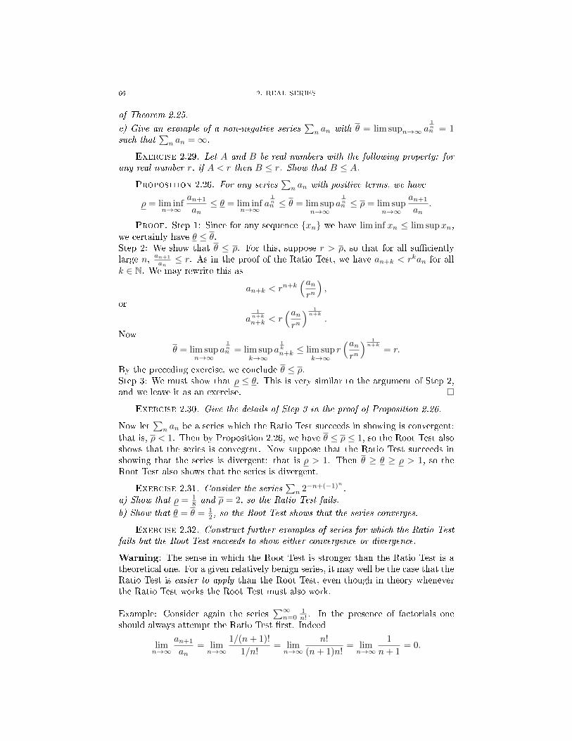
66 2. REAL SERIES

of Theorem 2.25.

c) Give an example of a non-negative series∑n an with θ = lim supn→∞ a

1nn = 1

such that∑n an =∞.

Exercise 2.29. Let A and B be real numbers with the following property: forany real number r, if A < r then B ≤ r. Show that B ≤ A.

Proposition 2.26. For any series∑n an with positive terms, we have

ρ = lim infn→∞

an+1

an≤ θ = lim inf

n→∞a

1nn ≤ θ = lim sup

n→∞a

1nn ≤ ρ = lim sup

n→∞

an+1

an.

Proof. Step 1: Since for any sequence {xn} we have lim inf xn ≤ lim supxn,we certainly have θ ≤ θ.Step 2: We show that θ ≤ ρ. For this, suppose r > ρ, so that for all su�cientlylarge n, an+1

an≤ r. As in the proof of the Ratio Test, we have an+k < rkan for all

k ∈ N. We may rewrite this as

an+k < rn+k(anrn

),

or

a1

n+k

n+k < r(anrn

) 1n+k

.

Now

θ = lim supn→∞

a1nn = lim sup

k→∞a

1k

n+k ≤ lim supk→∞

r(anrn

) 1n+k

= r.

By the preceding exercise, we conclude θ ≤ ρ.Step 3: We must show that ρ ≤ θ. This is very similar to the argument of Step 2,and we leave it as an exercise. �

Exercise 2.30. Give the details of Step 3 in the proof of Proposition 2.26.

Now let∑n an be a series which the Ratio Test succeeds in showing is convergent:

that is, ρ < 1. Then by Proposition 2.26, we have θ ≤ ρ ≤ 1, so the Root Test alsoshows that the series is convegent. Now suppose that the Ratio Test succeeds inshowing that the series is divergent: that is ρ > 1. Then θ ≥ θ ≥ ρ > 1, so theRoot Test also shows that the series is divergent.

Exercise 2.31. Consider the series∑n 2−n+(−1)n .

a) Show that ρ = 18 and ρ = 2, so the Ratio Test fails.

b) Show that θ = θ = 12 , so the Root Test shows that the series converges.

Exercise 2.32. Construct further examples of series for which the Ratio Testfails but the Root Test succeeds to show either convergence or divergence.

Warning: The sense in which the Root Test is stronger than the Ratio Test is atheoretical one. For a given relatively benign series, it may well be the case that theRatio Test is easier to apply than the Root Test, even though in theory wheneverthe Ratio Test works the Root Test must also work.

Example: Consider again the series∑∞n=0

1n! . In the presence of factorials one

should always attempt the Ratio Test �rst. Indeed

limn→∞

an+1

an= limn→∞

1/(n+ 1)!

1/n!= limn→∞

n!

(n+ 1)n!= limn→∞

1

n+ 1= 0.

6. SERIES WITH NON-NEGATIVE TERMS IV: STILL MORE CONVERGENCE TESTS 67

Thus the Ratio Test limit exists (no need for liminfs or limsups) and is equal to 0,so the series converges. If instead we tried the Root Test we would have to evaluatelimn→∞( 1

n! )1n . This is not so bad if we keep our head � e.g. one can show that for

any �xed R > 0 and su�ciently large n, n! > Rn and thus ( 1n! )

1n ≤ ( 1

Rn )1n = 1

R .

Thus the root test limit is at most 1R for any positive R, so it is 0. But this is

elaborate compared to the Ratio Test computation, which was immediate. In fact,turning these ideas around, Proposition 2.26 can be put to the following sneakyuse.

Corollary 2.27. Let {an}∞n=1 be a sequence of positive real numbers. Assume

that limn→∞an+1

an→ L ∈ [0,∞]. Then also limn→∞ a

1nn = L.

Proof. Indeed, the hypothesis gives that for the in�nite series∑n an we have

ρ = L, so by Proposition 2.26 we must also have θ = L!14 �

Exercise 2.33. Use Corollary 2.27 to evaluate the following limits:a) limn→∞ n

1n .

b) For α ∈ R, limn→∞ nαn .

c) limn→∞(n!)1n .

5.4. Remarks.

Parts a) and b) of the Ratio Test (Theorem 2.24) are due to d'Alembert.15 Theyimply parts c) and d), which is the version of the Ratio Test one meets in calculus,in which the limit is assumed to exist. As we saw above, it is equivalent to expressd'Alembert's Ratio Test in terms of lim sups and lim infs: this is the approachcommonly taken in contemporary undergraduate analysis texts. However, our de-cision to suppress the lim sups and lim infs was clinched by reading the treatmentof these tests in Hardy's16 classic text [H]. (He doesn't include the lim infs and limsups, his treatment is optimal, and his analytic pedigree is beyond reproach.)

Similarly, parts a) and b) of our Root Test (Theorem 2.25) are due to Cauchy.The reader can by now appreciate why calling it �Cauchy's Test� would not be agood idea. Similar remarks about the versions with lim sups apply, except that thistime, the result in part b) is actually stronger than the statement involving a limsup, as Exercise XX explores. Our statement of this part of the Root Test is takenfrom [H, §174].

6. Series With Non-Negative Terms IV: Still More Convergence Tests

If you are taking or teaching a �rst course on in�nite series / undergraduate analysis,I advise you to skip this section! It is rather for those who have seen the basicconvergence tests of the preceding sections many times over and who have startedto wonder what lies beyond.

14There is something decidedly strange about this argument: to show something about asequence {an} we reason in terms of the corresponding in�nite series

∑n an. But it works!

15Jean le Rond d'Alembert, 1717-178316Godfrey Harold Hardy, 1877-1947

68 2. REAL SERIES

6.1. The Ratio-Comparison Test.

Theorem 2.28. (Ratio-Comparison Test) Let∑n an,

∑n bn be two series

with positive terms. Suppose that there exists N ∈ Z+ such that for all n ≥ N wehave

an+1

an≤ bn+1

bn.

Then:a) If

∑n bn converges, then

∑n an converges.

b) If∑n an diverges, then

∑n bn converges.

Proof. As in the proof of the usual Ratio Test, for all k ∈ N,aN+k

aN=

aN+k

aN+k−1

aN+k−1

aN+k−2· · · aN+1

aN≤ bN+k

bN+k−1

bN+k−1

bN+k−2· · · bN+1

bN=bN+k

bN,

so

aN+k ≤(aNbN

)bN+k.

Now both parts follow by the Comparison Test. �

Warning: Some people use the term �Ratio Comparison Test� for what we (andmany others) have called the Limit Comparison Test.

Exercise 2.34. State and prove a Root-Comparison Test.

If we apply Theorem 2.28 by taking bn = rn for r < 1 and then an = rn for r > 1,we get the usual Ratio Test. It is an appealing idea to choose other series, or fami-lies of series, plug them into Theorem 2.28, and see whether we get other useful tests.

After the geometric series, perhaps our next favorite class of series with non-negativeterms are the p-series

∑n

1np . Let us �rst take p > 1, so that the p-series converges,

and put bn = 1np . Then our su�cient condition for the convergence of a series∑

n an with positive terms is

an+1

an≤ bn+1

bn=

(n+ 1)−p

n−p=

(n

n+ 1

)p=

(1− 1

n+ 1

)p.

Well, we have something here, but what? As is often the case for inequalities, it ishelpful to weaken it a bit to get something that is simpler and easier to apply (andthen perhaps come back later and try to squeeze more out of it).

Lemma 2.29. Let p > 0 and x ∈ [0, 1]. Then :a) If p > 1, then 1− px ≤ (1− x)p.b) If p < 1, then 1− px ≥ (1− x)p.

Proof. For x ∈ [0, 1], put f(x) = (1 − x)p − (1 − px). Then f is continuouson [0, 1], di�erentiable on [0, 1) with f(0) = 0. Moreover, for x ∈ [0, 1) we havef ′(x) = p(1− (1− x)p−1). Thus:a) If p > 1, f ′(x) ≥ 0 for all x ∈ [0, 1), so f is inceasing on [0, 1]. Since f(0) = 0,f(x) ≥ 0 for all x ∈ [0, 1].b) If 0 < p < 1, f ′(x) ≤ 0 for all x ∈ [0, 1), so f is decreasing on [0, 1]. Sincef(0) = 0, f(x) ≤ 0 for all x ∈ [0, 1]. �

6. SERIES WITH NON-NEGATIVE TERMS IV: STILL MORE CONVERGENCE TESTS 69

Remark: Although it was no trouble to prove Lemma 2.29, we should not neglectthe following question: how does one �gure out that such an inequality should exist?

The answer comes from the Taylor series expansion (1+x)α = 1+αx+α(α−1)2 x2+. . .

� the point being that the last term is positive when α > 1 and negative when0 < α < 1 � which will be discussed in the following chapter.

We are now in the position to derive a classic test due to J.L. Raabe.17

Theorem 2.30. (Raabe's Test)a) Let

∑n an be a series with positive terms. Suppose that for some p > 1 and all

su�ciently large n we have an+1

an≤ 1− p

n . Then∑n an <∞.

b) Let∑n bn be a series with positive terms. Suppose that for some 0 < p < 1 and

all su�ciently large n we have 1− pn ≤

bn+1

bn. Then

∑n bn =∞.

Proof. a) We have an+1

an≤ 1− p

n ≤ 1− pn+1 for all su�ciently large n. Applying

Lemma 2.29 with x = 1n+1 gives

an+1

an≤ 1− p

n+ 1≤(

1− 1

n+ 1

)p=bn+1

bn,

where bn = 1np . Since

∑n bn <∞,

∑n an <∞ by the Ratio-Comparison Test.

b) The proof is close enough to that of part a) to be left to the reader. �

Exercise 2.35. Prove Theorem 2.30b).

Theorem 2.30b) can be strengthened, as follows.

Theorem 2.31. Let∑n bn be a series with positive terms such that for all

su�ciently large n, bn ≥ 1− 1n . Then

∑n bn =∞.

Proof. We give two proofs.First proof: Let an = 1

n . Then an+1

an= 1 − 1

n and∑n an =

∑n

1n = ∞, so the

result follows from the Ratio-Comparison Test.

Second proof: We may assume bn+1

bn≥ 1 − 1

n for all n ∈ Z+. This is equivalent

to (n − 1)bn ≤ nbn+1 for all n ∈ Z+, i.e., the sequence nbn+1 is increasing and inparticular nbn+1 ≥ b2 > 0. Thus bn+1 ≥ b2

n and the series∑n bn+1 diverges by

comparison to the harmonic series. Of course this means∑n bn =∞ as well. �

Exercise 2.36. Show that Theorem 2.31 implies Theorem 2.30b).

Remark: We have just seen a proof of (a stronger form of) Theorem 2.30b) whichavoids the Ratio-Comparison Test. Similarly it is not di�cult to give a reasonablyshort, direct proof of Theorem 2.30a) depending on nothing more elaborate thanbasic comparison. In this way one gets an independent proof of the result that thep-series

∑n

1np diverges for p < 1 and converges for p > 1. However we do not get

a new proof of the p = 1 case, i.e., the divergence of the harmonic series (noticethat this was used, not proved, in the proof of Theorem 2.31). Ratio-like tests havea lot of trouble with the harmonic series!

The merit of the present approach is rather that it puts Raabe's test intoa larger context rather than just having it be one more test among many. Ourtreatment of Raabe's test is in�uenced by [Fa03].

17Joseph Ludwig Raabe, 1801-1859

70 2. REAL SERIES

6.2. Gauss's Test.

6.3. Kummer's Test.

6.4. Hypergeometric Series.

7. Absolute Convergence

7.1. Introduction to absolute convergence.

We turn now to the serious study of series with both positive and negative terms.It turns out that under one relatively mild additional hypothesis, virtually all ofour work on series with non-negative terms can be usefully applied in this case.In this section we study this wonderful hypothesis: absolute convergence. (In thenext section we get really serious by studying series when we do not have absoluteconvergence. As the reader will see, this leads to surprisingly delicate and intricateconsiderations: in practice, we very much hope that our series are absolutely con-vergent!)

A real series∑n an is absolutely convergent if

∑n |an| converges. Since

∑n |an|

is a series with non-negative terms, to determine absolute convergence we may useall the tools of the last three sections. A series

∑n an which converges but for

which∑n |an| diverges is said to be nonabsolutely convergent.18

The terminology absolutely convergent suggests that the convergence of the se-ries

∑n |an| is somehow �better� than the convergence of the series

∑n an. This is

indeed the case, although it is not obvious. But the following result already clari�esmatters a great deal.

Proposition 2.32. Every absolutely convergent series is convergent.

Proof. We shall give two proofs of this important result.First Proof : Consider the three series

∑n an,

∑n |an| and

∑n an + |an|. Our

hypothesis is that∑n |an| converges. But we claim that this implies that

∑n an +

|an| converges as well. Indeed, consider the expression an + |an|: it is equal to2an = 2|an| when an is non-negative and 0 when an is negative. In particular theseries

∑n an + |an| has non-negative terms and

∑n an + |an| ≤

∑n 2|an| <∞. So∑

n an + |an| converges. By the Three Series Principle,∑n an converges.

Second Proof : The above argument is clever � maybe too clever! Let's trysomething a little more fundamental: since

∑n |an| converges, for every ε > 0 there

exists N ∈ Z+ such that for all n ≥ N ,∑∞n=N |an| < ε. Therefore

|∞∑n=N

an| ≤∞∑n=N

|an| < ε,

and∑n an converges by the Cauchy criterion. �

18We warn the reader that the more standard terminology is conditionally convergent.We will later on give a separate de�nition for �conditionally convergent� and then it will be atheorem that a real series is conditionally convergent i� it is nonabsolutely convergent. Thereasoning for this � which we admit will seem abstruse at best to our target audience � is that infunctional analysis one studies convergence and absolute convergence of series in a more generalcontext, such that nonabsolute converge and conditional convergence may indeed di�er.

7. ABSOLUTE CONVERGENCE 71

Theorem 2.33. (N.J. Diepeveen) For an ordered �eld (F,<), the following areequivalent:(i) F is Cauchy-complete: every Cauchy sequence converges.(ii) Every absolutely convergent series in F is convergent.

Proof. (i) =⇒ (ii): This was done in the Second Proof of Proposition 2.32.(ii) =⇒ (i): Let {an} be a Cauchy sequence in F . A Cauchy sequence is con-vergent i� it admits a convergent subsequence, so it is enough to show that {an}admits a convergent subsequence. Like any sequence in an ordered set, {an} admitsa subsequence which is either constant, strictly increasing or strictly decreasing.A constant sequence is convergent, so we need not consider this case; moreover,a strictly decreasing sequence {an} converges i� the strictly increasing sequence{−an} converges, so we have reduced to the case in which {an} is strictly increas-ing:

a1 ≤ a2 ≤ . . . ≤ an ≤ . . . .For n ∈ Z+, put

bn = an+1 − an.Then bn > 0, and since {an} is Cauchy, bn → 0; thus we can extract a strictlydecreasing subsequence {bnk}. For k ∈ Z+, put

ck = bnk − bnk+1.

Then ck > 0 for all k and∞∑k=1

ck = bn1.

Since an is Cauchy, there exists for each k a positive integer mk such that

0 < amk+1− amk < ck.

For k ∈ Z+, put

d2k−1 = amk+1− amk , d2k = amk+1

− amk − ck.

We have

−ck < d2k < 0 < d2k−1 < ck,

so∞∑i=1

|di| =∞∑k=1

d2k−1 − d2k =

∞∑k=1

ck = bn1.

At last we get to use our hypothesis that absolutely convergent series are convergent:it follows that

∑∞i=1 di converges and

∞∑i=1

di +

∞∑k=1

ck =

∞∑k=1

(d2k−1 + d2k + ck) = 2

( ∞∑k=1

amk+1 − amk

).

Since, again, a Cauchy sequence with a convergent subsequence is itself convergent,

limn→∞

an = am1+

∞∑k=1

(amk+1− amk) = am1

+1

2

(bn1

+

∞∑i=1

di

).

�

For a more leisurely presentation of Theorem 2.33 and related topics, see [CD15].

72 2. REAL SERIES

Exercise 2.37. Find a sequence {an}∞n=1 of rational numbers such that∑∞n=1 |an|

is a rational number but∑∞n=1 an is an irrational number.

As an example of how Theorem 2.32 may be combined with the previous tests togive tests for absolute convergence, we record the following result.

Theorem 2.34. (Ratio & Root Tests for Absolute Convergence) Let∑n an be

a real series.a) Assume an 6= 0 for all n. If there exists 0 ≤ r < 1 such that for all su�cientlylarge n, |an+1

an| ≤ r, then the series

∑n an is absolutely convergent.

b) Assume an 6= 0 for all n. If there exists r > 1 such that for all su�ciently largen, |an+1

an| ≥ r, the series

∑n an is divergent.

c) If there exists r < 1 such that for all su�ciently large n, |an|1n ≤ r, the series∑

n an is absolutely convergent.

d) If there are in�nitely many n for which |an|1n ≥ 1, then the series diverges.

Proof. Parts a) and c) are immediate: applying Theorem 2.24 (resp. Theorem2.25) we �nd that

∑n |an| is convergent � and the point is that by Theorem 2.32,

this implies that∑n an is convergent.

There is something to say in parts b) and d), because in general just because∑n |an| = ∞ does not imply that

∑n an diverges. (We will study this subtlety

later on in detail.) But recall that whenever the Ratio or Root tests establish thedivergence of a non-negative series

∑n bn, they do so by showing that bn 9 0.

Thus under the hypotheses of parts b) and d) we have |an|9 0, hence also an 9 0so∑n an diverges by the Nth Term Test (Theorem 2.5). �

In particular, for a real series∑n an de�ne the following quantities:

ρ = limn→∞

|an+1

an| when it exists,

ρ = lim infn→∞

|an+1

an|,

ρ = lim supn→∞

|an+1

an|,

θ = limn→∞

|an|1n when it exists,

θ = lim supn→∞

|an|1n ,

and then all previous material on Ratio and Root Tests applies to all real series.

7.2. Cauchy products II: when one series is absolutely convergent.

Theorem 2.35. Let∑∞n=0 an = A and

∑∞n=0 bn = B be two absolutely conver-

gent series, and let cn =∑nk=0 akbn−k. Then the Cauchy product series

∑∞n=0 cn

is absolutely convergent, with sum AB.

Proof. We have proved this result already when an, bn ≥ 0 for all n. We wish,of course, to reduce to that case. As far as the convergence of the Cauchy product,this is completely straightforward: we have

∞∑n=0

|cn| =∞∑n=0

|n∑k=0

akbn−k| ≤∞∑n=0

n∑k=0

|ak||bn−k| <∞,

7. ABSOLUTE CONVERGENCE 73

the last inequality following from the fact that∑∞n=0

∑nk=0 |ak||bn−k| is the Cauchy

product of the two non-negative series∑∞n=0 |an| and

∑∞n=0 |bn|, hence it converges.

Therefore∑n |cn| converges by comparison, so the Cauchy product series

∑n cn

converges.We now wish to show that limN→∞ CN =

∑∞n=0 cn = AB. Recall the notation

�N =∑

0≤i,j≤N

aibj = (a0 + . . .+ aN )(b0 + . . .+ bN ) = ANBN .

We have

|CN −AB| ≤ |�N −AB|+ |�N − CN |= |ANBN −AB|+ |a1bN |+ |a2bN−1|+ |a2bN |+ . . .+ |aNb1|+ . . .+ |aNbN |

≤ |ANBN −AB|+

( ∞∑n=0

|an|

)∑n≥N

|bn|

+

( ∞∑n=0

|bn|

)∑n≥N

|an|

.

Fix ε > 0; since ANBN → AB, for su�ciently large N |ANBN −AB| < ε3 . Put

A =

∞∑n=0

|an|, B =

∞∑n=0

|bn|.

By the Cauchy criterion, for su�ciently large N we have∑n≥N |bn| <

ε3A and∑

n≥N |an| <ε3B and thus |CN −AB| < ε. �

While the proof of Theorem 2.35 may seem rather long, it is in fact a rather straight-forward argument: one shows that the di�erence between the box product and thepartial sums of the Cauchy product becomes negligible as N tends to in�nity. Inless space but with a bit more �nesse, one can prove the following stronger result,a theorem of F. Mertens [Me72].19

Theorem 2.36. (Mertens' Theorem) Let∑∞n=0 an = A be an absolutely con-

vegent series and∑∞n=0 bn = B be a convergent series. Then the Cauchy product

series∑∞n=0 cn converges to AB.

Proof. (Rudin [R, Thm. 3.50]): de�ne (as usual)

AN =

N∑n=0

an, BN =

N∑n=0

bn, CN =

N∑n=0

cn

and also (for the �rst time)

βn = Bn −B.Then for all N ∈ N,

CN = a0b0 + (a0b1 + a1b0) + . . .+ (a0bN + . . .+ aNb0)

= a0BN + a1BN−1 + . . .+ aNB0

= a0(B + βN ) + a1(B + βN−1) + . . .+ aN (B + β0)

= ANB + a0βN + a1βN−1 + . . .+ aNβ0 = ANB + γN ,

say, where γN = a0βN + a1βN−1 + . . . + anβ0. Since our goal is to show thatCN → AB and we know that ANB → AB, it su�ces to show that γN → 0. Now,

19Franz Carl Joseph Mertens, 1840-1927

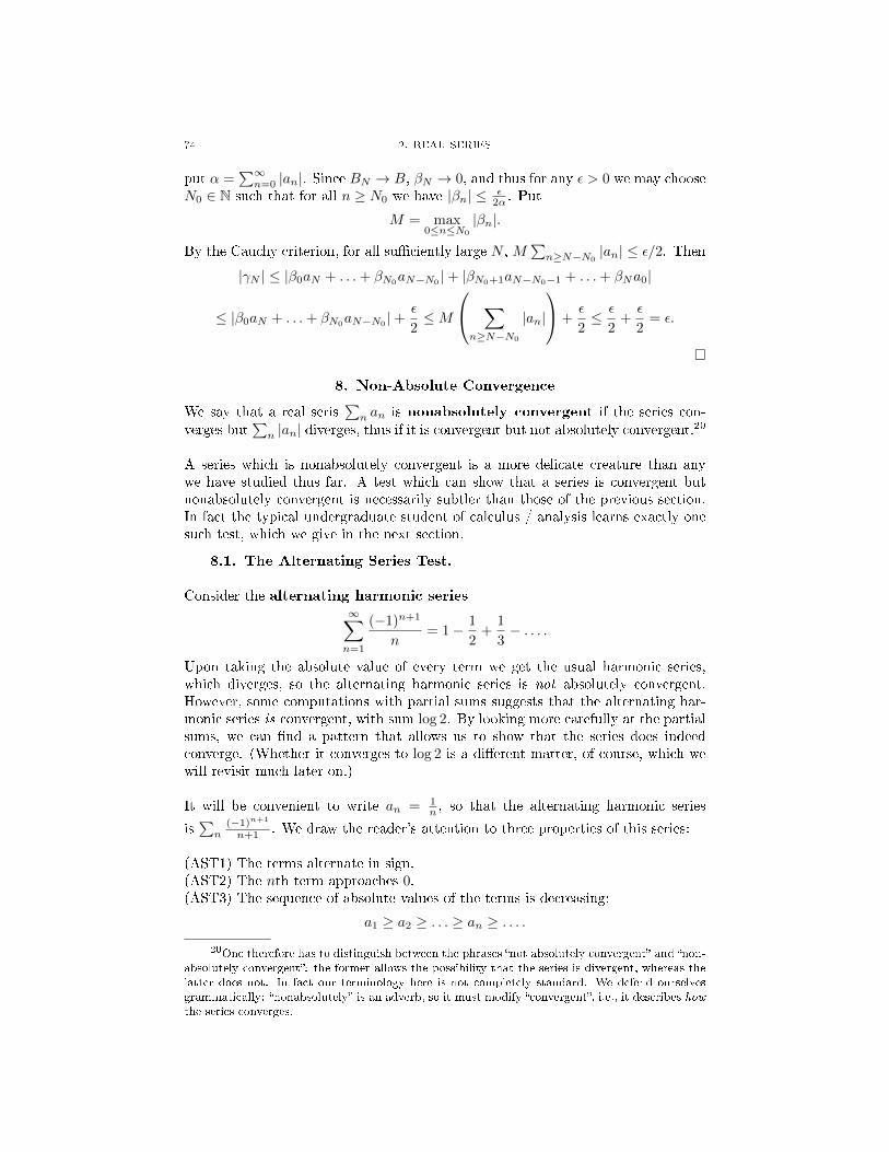
74 2. REAL SERIES

put α =∑∞n=0 |an|. Since BN → B, βN → 0, and thus for any ε > 0 we may choose

N0 ∈ N such that for all n ≥ N0 we have |βn| ≤ ε2α . Put

M = max0≤n≤N0

|βn|.

By the Cauchy criterion, for all su�ciently large N , M∑n≥N−N0

|an| ≤ ε/2. Then

|γN | ≤ |β0aN + . . .+ βN0aN−N0

|+ |βN0+1aN−N0−1 + . . .+ βNa0|

≤ |β0aN + . . .+ βN0aN−N0

|+ ε

2≤M

∑n≥N−N0

|an|

+ε

2≤ ε

2+ε

2= ε.

�

8. Non-Absolute Convergence

We say that a real seris∑n an is nonabsolutely convergent if the series con-

verges but∑n |an| diverges, thus if it is convergent but not absolutely convergent.

20

A series which is nonabsolutely convergent is a more delicate creature than anywe have studied thus far. A test which can show that a series is convergent butnonabsolutely convergent is necessarily subtler than those of the previous section.In fact the typical undergraduate student of calculus / analysis learns exactly onesuch test, which we give in the next section.

8.1. The Alternating Series Test.

Consider the alternating harmonic series∞∑n=1

(−1)n+1

n= 1− 1

2+

1

3− . . . .

Upon taking the absolute value of every term we get the usual harmonic series,which diverges, so the alternating harmonic series is not absolutely convergent.However, some computations with partial sums suggests that the alternating har-monic series is convergent, with sum log 2. By looking more carefully at the partialsums, we can �nd a pattern that allows us to show that the series does indeedconverge. (Whether it converges to log 2 is a di�erent matter, of course, which wewill revisit much later on.)

It will be convenient to write an = 1n , so that the alternating harmonic series

is∑n

(−1)n+1

n+1 . We draw the reader's attention to three properties of this series:

(AST1) The terms alternate in sign.(AST2) The nth term approaches 0.(AST3) The sequence of absolute values of the terms is decreasing:

a1 ≥ a2 ≥ . . . ≥ an ≥ . . . .

20One therefore has to distinguish between the phrases �not absolutely convergent� and �non-absolutely convergent�: the former allows the possibility that the series is divergent, whereas thelatter does not. In fact our terminology here is not completely standard. We defend ourselvesgrammatically: �nonabsolutely� is an adverb, so it must modify �convergent�, i.e., it describes howthe series converges.

8. NON-ABSOLUTE CONVERGENCE 75

These are the clues from which we will make our case for convergence. Here it is:consider the process of passing from the �rst partial sum S1 = 1 to S3 = 1− 1

2 + 13 =

56 . We have S3 ≤ 1, and this is no accident: since a2 ≥ a3, subtracting a2 and thenadding a3 leaves us no larger than where we started. But indeed this argument isvalid in passing from any S2n−1 to S2n+1:

S2n+1 = S2n−1 − a2n + a2n+1 ≤ S2n+1.

It follows that the sequence of odd-numbered partial sums {S2n−1} is decreasing.Moreover,

S2n+1 = (a1 − a2) + (a3 − a4) + . . .+ (a2n−1| − |a2n) + a2n−1 ≥ 0.

Therefore all the odd-numbered terms are bounded below by 0. By the MonotoneSequence Lemma, the sequence {S2n+1} converges to its greatest lower bound, saySodd. On the other hand, just the opposite sort of thing happens for the even-numbered partial sums:

S2n+2 = S2n + a2n+1 − a2n+2 ≥ S2n

and

S2n+2 = a1 − (a2 − a3)− (a4 − a5)− . . .− (a2n − a2n+1|)− a2n+2 ≤ a1.

Therfore the sequence of even-numbered partial sums {S2n} is increasing andbounded above by a1, so it converges to its least upper bound, say Seven. Thus wehave split up our sequence of partial sums into two complementary subsequencesand found that each of these series converges. By X.X, the full sequence {Sn}converges i� Sodd = Seven. Now the inequalities

S2 ≤ S4 ≤ . . . ≤ S2n ≤ S2n+1 ≤ S2n−1 ≤ . . . ≤ S3 ≤ S1

show that Seven ≤ Sodd. Moreover, for any n ∈ Z+ we have

Sodd − Seven ≤ S2n+1 − S2n = a2n+1.

Since a2n+1 → 0, we conclude Sodd = Seven = S, i.e., the series converges.

In fact these inequalities give something else: since for all n we have S2n ≤ S2n+2 ≤S ≤ S2n+1, it follows that

|S − S2n| = S − S2n ≤ S2n+1 − S2n = a2n+1

and similarly

|S − S2n+1| = S2n+1 − S ≤ S2n+1 − S2n+2 = a2n+2.

Thus the error in cutting o� the in�nite sum∑∞n=1(−1)n+1|an| after N terms is in

absolute value at most the absolute value of the next term: aN+1.

Of course in all this we never used that an = 1n but only that we had a series

satisfying (AST1) (i.e., an alternating series), (AST2) and (AST3). Therefore thepreceding arguments have in fact proved the following more general result, dueoriginally due to Leibniz.21

21Gottfried Wilhelm von Leibniz, 1646-1716

76 2. REAL SERIES

Theorem 2.37. (Lebniz's Alternating Series Test) Let {an}∞n=1 be a sequenceof non-negative real numbers which is decreasing and such that limn→∞ an = 0.Then:a) The associated alternating series

∑n(−1)n+1an converges.

b) For N ∈ Z+, put

(14) EN = |(∞∑n=1

(−1)n+1an)− (

N∑n=1

(−1)n+1an)|,

the �error� obtained by cutting o� the in�nite sum after N terms. Then we havethe error estimate

EN ≤ aN+1.

Exercise 2.38. Let p ∈ R: Show that the alternating p-series∑∞n=1

(−1)n+1

np

is:(i) divergent if p ≤ 0,(ii) nonabsolutely convergent if 0 < p ≤ 1, and(iii) absolutely convergent if p > 1.

Exercise 2.39. Let P (x)Q(x) be a rational function. Give necessary and su�cient

conditions for∑n(−1)n P (x)

Q(x) to be nonabsolutely convergent.

For any convergent series∑∞n=1 an = S, we may de�ne EN as in (14) above:

EN = |S −N∑n=1

an|.

Then because the series converges to S, limN→∞EN = 0, and conversely: in otherwords, to say that the error goes to 0 is a rephrasing of the fact that the partialsums of the series converge to S. Each of these statements is (in the jargon ofmathematicians working in this area) soft: we assert that a quantity approaches 0and N →∞, so that in theory, given any ε > 0, we have EN < ε for all su�ucientlylarge N . But as we have by now seen many times, it is often possible to show thatEN → 0 without coming up with an explicit expression for N in terms of ε. Butthis stronger statement is exactly what we have given in Theorem 2.37b): we havegiven an explicit upper bound on EN as a function of N . This type of statementis called a hard statement or an explicit error estimate: such statements tendto be more di�cult to come by than soft statements, but also more useful to have.Here, as long as we can similarly make explicit how large N has to be in order foraN to be less than a given ε > 0, we get a completely explicit error estimate andcan use this to actually compute the sum S to arbitrary accuracy.

Example: We compute∑∞n=1

(−1)n+1

n to three decimal place accuracy. (Let usagree that to �compute a number α to k decimal place accuracy means to computeit with error less than 10−k. A little thought shows that this is not quite enough toguarantee that the �rst k decimal places of the approximation are equal to the �rstk decimal places of α, but we do not want to occupy ourselves with such issues here.)By Theorem 2.37b), it is enough to �nd an N ∈ Z+ such that aN+1 = 1

N+1 <1

1000 .


We may take N = 1000. Therefore

|∞∑n=1

(−1)n+1

n−

1000∑n=1

(−1)n+1

n| ≤ 1

1001.

Using a software package, we �nd that

1000∑n=1

(−1)n+1

n= 0.6926474305598203096672310589 . . . .

Again, later we will show that the exact value of the sum is log 2, which my softwarepackage tells me is22

log 2 = 0.6931471805599453094172321214.

Thus the actual error in cutting o� the sum after 1000 terms is

E1000 = 0.0004997500001249997500010625033.

It is important to remember that this and other error estimates only give upperbounds on the error: the true error could well be much smaller. In this case wewere guaranteed to have an error at most 1

1001 and we see that the true error isabout half of that. Thus the estimate for the error is reasonably accurate.

Note well that although the error estimate of Theorem 2.37b) is very easy toapply, if an tends to zero rather slowly (as in this example), it is not especiallye�cient for computations. For instance, in order to compute the true sum of thealternating harmonic series to six decimal place accuracy using this method, wewould need to add up the �rst million terms: that's a lot of calculation. (Thusplease be assured that this is not the way that a calculator or computer wouldcompute log 2.)

Example: We compute∑∞n=0

(−1)nn! to six decimal place accuracy. Thus we need to

chooseN such that aN+1 = 1(N+1)! < 10−6, or equivalently such that (N+1)! > 106.

A little calculation shows 9! = 362, 880 and 10! = 3, 628, 800, so that we may takeN = 9 (but not N = 8). Therefore

|∞∑n=0

(−1)n

n!−

9∑n=0

(−1)n

n!| < 1

10!< 10−6.

Using a software package, we �nd

9∑n=0

(−1)n

n!= 0.3678791887125220458553791887.

In this case the exact value of the series is1

e== 0.3678794411714423215955237701

so the true error is

E9 = 0.0000002524589202757401445814516374,

which this time is only very slightly less than the guaranteed

1

10!= 0.0000002755731922398589065255731922.

22Yes, you should be wondering how it is computing this! More on this later.

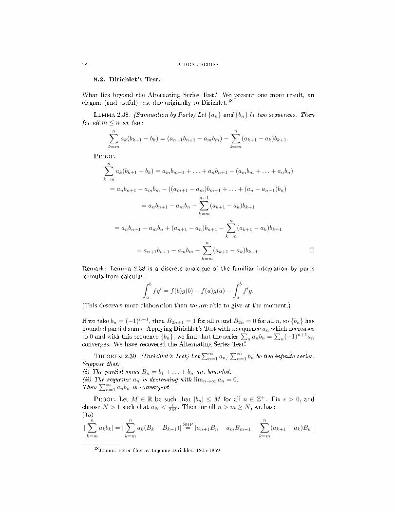
78 2. REAL SERIES

8.2. Dirichlet's Test.

What lies beyond the Alternating Series Test? We present one more result, anelegant (and useful) test due originally to Dirichlet.23

Lemma 2.38. (Summation by Parts) Let {an} and {bn} be two sequences. Thenfor all m ≤ n we have

n∑k=m

ak(bk+1 − bk) = (an+1bn+1 − ambm)−n∑

k=m

(ak+1 − ak)bk+1.

Proof.n∑

k=m

ak(bk+1 − bk) = ambm+1 + . . .+ anbn+1 − (ambm + . . .+ anbn)

= anbn+1 − ambm − ((am+1 − am)bm+1 + . . .+ (an − an−1)bn)

= anbn+1 − ambn −n−1∑k=m

(ak+1 − ak)bk+1

= anbn+1 − ambn + (an+1 − an)bn+1 −n∑

k=m

(ak+1 − ak)bk+1

= an+1bn+1 − ambm −n∑

k=m

(ak+1 − ak)bk+1. �

Remark: Lemma 2.38 is a discrete analogue of the familiar integration by partsformula from calculus:∫ b

a

fg′ = f(b)g(b)− f(a)g(a)−∫ b

a

f ′g.

(This deserves more elaboration than we are able to give at the moment.)

If we take bn = (−1)n+1, then B2n+1 = 1 for all n and B2n = 0 for all n, so {bn} hasbounded partial sums. Applying Dirichlet's Test with a sequence an which decreasesto 0 and with this sequence {bn}, we �nd that the series

∑n anbn =

∑n(−1)n+1an

converges. We have recovered the Alternating Series Test!

Theorem 2.39. (Dirichlet's Test) Let∑∞n=1 an,

∑∞n=1 bn be two in�nite series.

Suppose that:(i) The partial sums Bn = b1 + . . .+ bn are bounded.(ii) The sequence an is decreasing with limn→∞ an = 0.Then

∑∞n=1 anbn is convergent.

Proof. Let M ∈ R be such that |bn| ≤ M for all n ∈ Z+. Fix ε > 0, andchoose N > 1 such that aN < ε

2M . Then for all n > m ≥ N , we have(15)

|n∑

k=m

akbk| = |n∑

k=m

ak(Bk −Bk−1)| SBP= |an+1Bn − amBm−1 −

n∑k=m

(ak+1 − ak)Bk|

23Johann Peter Gustav Lejeune Dirichlet, 1805-1859


≤M

(an+1 + am +

n∑k=m

(ak+1 − ak)

)

= M (an+1 + am + an+1 − am) = 2Man+1 ≤ 2MaN < ε.

Therefore∑n anbn converges by the Cauchy criterion. �

Exercise 2.40. a) Show: Dirichlet's Test implies the Alternating Series Test.b) Show: Dirichlet's Test implies the Almost Alternating Series Test: let {an}be a sequence decreasing to 0, and for all n ∈ Z+ let bn ∈ {±1} be a sign sequencewhich is �almost alternating� in the sense that the sequence of partial sums Bn =b1 + . . .+ bn is bounded. Then the series

∑n bnan converges.

Exercise 2.41. Show that Dirichlet's generalization of the Alternating SeriesTest is �as strong as possible� in the following sense: if {bn} is a sequence ofelements, each ±1, such that the sequence of partial sums Bn = b1 + . . . + bnis unbounded, then there is a sequence an decreasing to zero such that

∑n anbn

diverges.

Exercise 2.42. a) Use the trigonometric identity24

cosn =sin(n+ 1

2 )− sin(n− 12 )

2 sin( 12 )

to show that the sequence Bn = cos 1 + . . .+ cosn is bounded.b) Apply Dirichlet's Test to show that the series

∑∞n=1

cosnn converges.

c) Show that∑∞n=1

cosnn is not absolutely convergent.

Exercise 2.43. Show:∑∞n=1

sinnn is nonabsolutely convergent.

Remark: Once we know about series of complex numbers and Euler's formulaeix = cosx+ i sinx, we will be able to give a �trigonometry-free� proof of the pre-ceding two exercises.

Dirichlet himself applied his test to establish the convergence of a certain classof series of a mixed algebraic and number-theoretic nature. The analytic proper-ties of these series were used to prove his celebrated theorem on prime numbers inarithmetic progressions. To give a sense of how in�uential this work has become, inmodern terminology Dirichlet studied the analytic properties of Dirichlet seriesassociated to nontrivial Dirichlet characters. For more information on this work,the reader may consult (for instance) [DS].

A real sequence {an} has bounded variation if

∞∑n=1

|an+1 − an| <∞.

Proposition 2.40. If the real sequence {an} has bounded variation, then it isconvergent.

24An instance of the sum-product identities. Yes, I hardly remember them either.

80 2. REAL SERIES

Proof. Fix ε > 0, and choose N ∈ Z+ such that∑n≥N |an+1−an| < ε. Then

for all N ≤ m ≤ n we have

|an−am| = |(an−an−1)+. . .+(am+1−am)| ≤n−1∑i=m

|ai+1−ai| ≤∑n≥N

|an+1−an| < ε.

Therefore the sequence {an} is Cauchy, hence convergent. �

Theorem 2.41. (Dedekind's Test) Let {an} be a real sequence with boundedvariation, and let

∑∞n=1 bn be a convergent real series. Then

∑∞n=1 anbn converges.

Exercise 2.44. Prove Dedekind's Test.(Suggestion: Proceed as in the proof of Dirichlet's Test, using (15).)

Theorem 2.42. (Abel's Test) Let {an} be a bounded monotone real sequence,and let

∑∞n=1 bn be a convergent real series. Then

∑∞n=1 anbn converges.

Exercise 2.45.a) Show that a monotone sequence {an} has bounded variation i� it is bounded.b) Deduce Abel's Test from Dedekind's Test.c) Deduce Abel's Test from Dirichlet's Test.(Suggestion: In the notation of Abel's Test, suppose that an → a. Replace {an}with {an − a} to apply Dirichlet's Test.)

Exercise 2.46.a) Let {an} and {bn} be real sequences of bounded variation, and let α, β ∈ R.Show: {αan + βbn} has bounded variation.b) Show: if

∑n an is absolutely convergent, then {an} has bounded variation.

c) Show: for every real sequence {an} there are increasing sequences {bn} and {cn}such that {an} = {bn} − {cn}.d) Show: for a real sequence {an}, the following are equivalent:(i) {an} has bounded variation.(ii) There are bounded increasing sequences {bn} and {cn} such that {an} = {bn}−{cn}.

8.3. A divergent Cauchy product.

Recall that we showed that if∑n an = A and

∑n bn = B are convergent se-

ries, at least one of which is absolutely convergent, then the Cauchy product series∑n cn is convergent to AB. Here we give an example � due to Cauchy! � of a

Cauchy product of two nonabsolutely convergent series which fails to converge.

We will take∑∞n=0 an =

∑∞n=0 bn =

∑∞n=0

(−1)n√n+1

. (The series is convergent by

the Alternating Series Test.) The nth term in the Cauchy product is

cn =∑i+j=n

(−1)i(−1)j1√i+ 1

1√j + 1

.

The �rst thing to notice is (−1)i(−1)j = (−1)i+j = (−1)n, so cn is equal to (−1)n

times a sum of positive terms. We have i, j ≤ n so 1√i+1

, 1√j+1≥ 1√

n+1, and thus

each term in cn has absolute value at least ( 1√n+1

)2 = 1n+1 . Since we are summing

from i = 0 to n there are n+ 1 terms, all of the same size, we �nd |cn| ≥ 1 for alln. Thus the general term of

∑n cn does not converge to 0, so the series diverges.

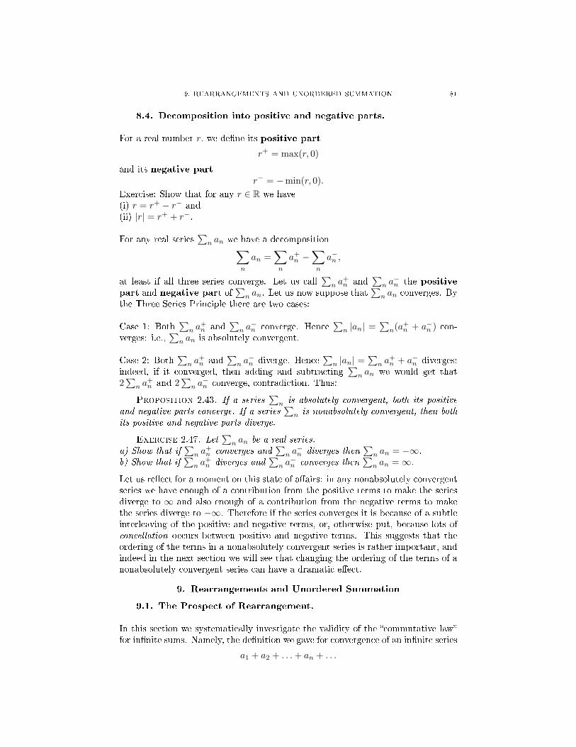
9. REARRANGEMENTS AND UNORDERED SUMMATION 81

8.4. Decomposition into positive and negative parts.

For a real number r, we de�ne its positive part

r+ = max(r, 0)

and its negative partr− = −min(r, 0).

Exercise: Show that for any r ∈ R we have(i) r = r+ − r− and(ii) |r| = r+ + r−.

For any real series∑n an we have a decomposition∑

n

an =∑n

a+n −∑n

a−n ,

at least if all three series converge. Let us call∑n a

+n and

∑n a−n the positive

part and negative part of∑n an. Let us now suppose that

∑n an converges. By

the Three Series Principle there are two cases:

Case 1: Both∑n a

+n and

∑n a−n converge. Hence

∑n |an| =

∑n(a+n + a−n ) con-

verges: i.e.,∑n an is absolutely convergent.

Case 2: Both∑n a

+n and

∑n a−n diverge. Hence

∑n |an| =

∑n a

+n + a−n diverges:

indeed, if it converged, then adding and subtracting∑n an we would get that

2∑n a

+n and 2

∑n a−n converge, contradiction. Thus:

Proposition 2.43. If a series∑n is absolutely convergent, both its positive

and negative parts converge. If a series∑n is nonabsolutely convergent, then both

its positive and negative parts diverge.

Exercise 2.47. Let∑n an be a real series.

a) Show that if∑n a

+n converges and

∑n a−n diverges then

∑n an = −∞.

b) Show that if∑n a

+n diverges and

∑n a−n converges then

∑n an =∞.

Let us re�ect for a moment on this state of a�airs: in any nonabsolutely convergentseries we have enough of a contribution from the positive terms to make the seriesdiverge to ∞ and also enough of a contribution from the negative terms to makethe series diverge to −∞. Therefore if the series converges it is because of a subtleinterleaving of the positive and negative terms, or, otherwise put, because lots ofcancellation occurs between positive and negative terms. This suggests that theordering of the terms in a nonabsolutely convergent series is rather important, andindeed in the next section we will see that changing the ordering of the terms of anonabsolutely convergent series can have a dramatic e�ect.

9. Rearrangements and Unordered Summation

9.1. The Prospect of Rearrangement.

In this section we systematically investigate the validity of the �commutative law�for in�nite sums. Namely, the de�nition we gave for convergence of an in�nite series

a1 + a2 + . . .+ an + . . .

82 2. REAL SERIES

in terms of the limit of the sequence of partial sums An = a1 + . . . + an makesat least apparent use of the ordering of the terms of the series. Note that this issomewhat surprising even from the perspective of in�nite sequences: the statementan → L can be expressed as: for all ε > 0, there are only �nitely many terms of thesequence lying outside the interval (L − ε, L + ε), a description which makes clearthat convergence to L will not be a�ected by any reordering of the terms of thesequence. However, if we reorder the terms {an} of an in�nite series

∑∞n=1 an, the

corresponding change in the sequence An of partial sums is not simply a reordering,as one can see by looking at very simple examples. For instance, if we reorder

1

2+

1

4+

1

8+ . . .+

1

2n+ . . .

as1

4+

1

2+

1

8+ . . .+

1

2n+ . . .

Then the �rst partial sum of the new series is 14 , whereas every nonzero partial sum

of the original series is at least 12 .

Thus there is some evidence to fuel suspicion that reordering the terms of an in�-nite series may not be so innocuous an operation as for that of an in�nite seuqence.All of this discussion is mainly justi�cation for our setting up the �rearrangementproblem� carefully, with a precision that might otherwise look merely pedantic.

Namely, the formal notion of rearrangement of a series∑∞n=0 an begins with a

permuation σ of N, i.e., a bijective function σ : N→ N. We de�ne the rearrange-ment of

∑∞n=0 an by σ to be the series

∑∞n=0 aσ(n).

9.2. The Rearrangement Theorems of Weierstrass and Riemann.

The most basic questions on rearrangements of series are as follows.

Question 2.44. Let∑∞n=0 an = S is a convergent in�nite series, and let σ be

a permutation of N. Then:a) Does the rearranged series

∑∞n=0 aσ(n) converge?

b) If it does converge, does it converge to S?

As usual, the special case in which all terms are non-negative is easiest, the caseof absolute convergence is not much harder than that, and the case of nonabsoluteconvergence is where all the real richness and subtlety lies.

Indeed, suppose that an ≥ 0 for all n. In this case the sum A =∑∞n=0 an ∈ [0,∞

is simply the supremum of the set An =∑kn=0 ak of �nite sums. More gener-

ally, let S = {n1, . . . , nk} be any �nite subset of the natural numbers, and putAS = an1 + . . .+ ank . Now every �nite subset S ⊂ N is contained in {0, . . . , N} forsome N ∈ N, so for all S, AS ≤ AN for some (indeed, for all su�ciently large) N .This shows that if we de�ne

A′ = supSAS

as S ranges over all �nite subsets of N, then A′ ≤ A. On the other hand, for allN ∈ N, AN = a0 + . . . + aN = A{0,...,N}: in other words, each partial sum ANarises as AS for a suitable �nite subset S. Therefore A ≤ A′ and thus A = A′.


The point here is that the description∑∞n=0 an = supS AS is manifestly unchanged

by rearranging the terms of the series by any permutation σ: taking S 7→ σ(S)gives a bijection on the set of all �nite subsets of N, and thus

∞∑n=0

an = supSAS = sup

SAσ(S) =

∞∑n=0

aσ(n).

The case of absolutely convergent series follows rather easily from this.

Theorem 2.45. (Weierstrass) Let∑∞n=0 an be an absolutely convergent series

with sum A. Then for every permutation σ of N, the rearranged series∑∞n=0 aσ(n)

converges to A.

Proof. For N ∈ Z+, de�ne

Nσ = max0≤k<N

σ−1(k).

In other words, Nσ is the least natural number such that σ({0, 1, . . . , Nσ}) ⊇{0, 1, . . . , N − 1}. Thus for n > Nσ, σ(n) ≥ N . For all ε > 0, by the Cauchycriterion for absolute convergence, there is N ∈ N with

∑∞n=N |an| < ε. Then

∞∑n=Nσ+1

|aσ(n)| ≤∞∑n=N

|an| < ε,

and the rearranged series is absolutely convergent by the Cauchy criterion. LetA′ =

∑∞n=0 aσ(n). Then

|A−A′| ≤ |Nσ∑n=0

an − aσ(n)|+∑n>Nσ

|an|+∑n>Nσ

|aσ(n)| < |Nσ∑n=0

an − aσ(n)|+ 2ε.

Moreover, each term ak with 0 ≤ k ≤ N appears in both∑Nσn=0 an and

∑Nσn=0 aσ(n),

so we may make the very crude estimate

|Nσ∑n=0

an − aσ(n)| ≤ 2∑n>N

|an| < 2ε

which gives

|A−A′| < 4ε.

Since ε was arbitrary, we conclude A = A′. �

Exercise 2.48. Use the decomposition of∑n an into its series of positive parts∑

n a+n and negative parts

∑n a−n to give a second proof of Theorem 2.45.

Theorem 2.46. (Riemann Rearrangement Theorem) Let∑∞n=0 an be a non-

absolutely convergent series. For any B ∈ [−∞,∞], there exists a permutation σof N such that

∑∞n=0 aσ(n) = B.

Proof.

Step 1: Since∑n an is convergent, we have an → 0 and thus that {an} is bounded,

so we may choose M such that |an| ≤ M for all n. We are not going to give anexplicit �formula� for σ; rather, we are going to describe σ by a certain process.For this it is convenient to imagine that the sequence {an} has been sifted into adisjoint union of two subsequences, one consisting of the positive terms and one

84 2. REAL SERIES

consisting of the negative terms (we may assume without loss of generality thatthere an 6= 0 for all n). If we like, we may even imagine both of these subseqeunceordered so that they are decreasing in absolute value. Thus we have two sequences

p1 ≥ p2 ≥ . . . ≥ pn ≥ . . . ≥ 0,

n1 ≤ n2 ≤ . . . ≤ nn ≤ . . . ≤ 0

so that together {pn, nn} comprise the terms of the series. The key point here isProposition 2.43 which tells us that since the convergence is nonabsolute,

∑n pn =

∞,∑n nn = −∞. So we may specify a rearangement as follows: we specify a

choice of a certain number of positive terms � taken in decreasing order � and thena choice of a certain number of negative terms � taken in order of decreasing ab-solute value � and then a certain number of positive terms, and so on. As long aswe include a �nite, positive number of terms at each step, then in the end we willhave included every term pn and nn eventually, hence we will get a rearrangement.

Step 2 (diverging to∞): to get a rearrangement diverging to∞, we proceed asfollows: we take positive terms p1, p2, . . . in order until we arrive at a partial sumwhich is at least M + 1; then we take the �rst negative term n1. Since |n1| ≤ M ,the partial sum p1 + . . . + pN1 + n1 is still at least 1. Then we take at least onemore positive term pN1+1 and possibly further terms until we arrive at a partialsum which is at least M + 2. Then we take one more negative term n2, and notethat the partial sum is still at least 2. And we continue in this manner: after thekth step we have used at least k positive terms, at least k negative terms, and allthe partial sums from that point on will be at least k. Therefore every term getsincluded eventually and the sequence of partial sums diverges to +∞.

Step 3 (diverging to −∞): An easy adaptation of the argument of Step 2 leadsto a permutation σ such that

∑∞n=0 aσ(n) = −∞. We leave this case to the reader.

Step 4 (converging to B ∈ R): if anything, the argument is simpler in this case. We�rst take positive terms p1, . . . , pN1

, stopping when the partial sum p1 + . . .+ pN1

is greater than B. (To be sure, we take at least one positive term, even if 0 >B.) Then we take negative terms n1, . . . , nN2

, stopping when the partial sump1 + . . .+ pN1 + n1 + . . .+ nN2 is less than B. Then we repeat the process, takingenough positive terms to get a sum strictly larger than B then enough negativeterms to get a sum strictly less than B, and so forth. Because both the positiveand negative parts diverge, this construction can be completed. Because the gen-eral term an → 0, a little thought shows that the absolute value of the di�erencebetween the partial sums of the series and B approaches zero. �

Exercise 2.49. Fill in the omitted details in the proof of Theorem 2.46. Inparticular:a) Construct a permutation σ of N such that

∑n aσ(n) → −∞.

b) Show that the rearranged series of Step 4 does indeed converge to B. (Suggestion:it may be helpful to think of the rearrangement process as a walk along the real line,taking a certain number of steps in a positive direction and then a certain numberof steps in a negative direction, and so forth. The key point is that by hypothesisthe step size is approaching zero, so the amount by which we �overshoot� the limitB at each stage decreases to zero.)


The fact that the original series∑n an converges was not used very strongly in the

proof. The following exercises deduce the same conclusions of Theorem 2.46 undermilder hypotheses.

Exercise 2.50. Let∑n an be a real series such that an → 0,

∑n a

+n = ∞

and∑n a−n = −∞. Show that the conclusion of Theorem 2.46 holds: for any

A ∈ [−∞,∞], there exists a permutation σ of N such that∑∞n=0 aσ(n) = A.

Exercise 2.51. Let∑n an be a real series such that

∑n a

+n =∞.

a) Suppose that the sequence {an} is bounded. Show that there exists a permutationσ of N such that

∑n aσ(n) =∞.

b) Does the conclusion of part a) hold without the assumption that the sequnece ofterms is bounded?

Theorem 2.46 exposes the dark side of nonabsolutely convergent series: just bychanging the order of the terms, we can make the series diverge to ±∞ or convergeto any given real number! Thus nonabsolute convergence is necessarily of a moredelicate and less satisfactory nature than absolute convergence. With these issuesin mind, we de�ne a series

∑n an to be unconditionally convergent if it is

convergent and every rearrangement converges to the same sum, and a series to beconditionally convergent if it is convergent but not unconditionally convergent.Then much of our last two theorems may be summarized as follows.

Theorem 2.47. (Main Rearrangement Theorem) A convergent real series isunconditionally convergent i� it is absolutely convergent.

Many texts do not use the term �nonabsolutely convergent� and instead de�ne a se-ries to be conditionally convergent if it is convergent but not absolutely convergent.Aside from the fact that this terminology can be confusing to students (especiallycalculus students) to whom this rather intricate story of rearrangements has notbeen told, it seems correct to make a distinction between the following two a prioridi�erent phenomena:

•∑n an converges but

∑n |an| does not, versus

•∑n an converges to A but some rearrangement

∑n aσ(n) does not.

Now it happens that these two phenomena are equivalent for real series. How-ever the notion of an in�nite series

∑n an, absolute and unconditional convergence

makes sense in other contexts as well, for instance for series with values in anin�nite-dimensional Banach space or with values in a p-adic �eld. In the for-mer case it is a celebrated theorem of Dvoretsky-Rogers [DR50] that there exists aseries which is unconditionally convergent but not absolutely convergent, whereasin the latter case one can show that every convergent series is unconditionallyconvergent whereas there exist nonabsolutely convergent series.

Exercise 2.52. Let∑∞n=0 an be any nonabsolutely convergent real series, and

let −∞ ≤ a ≤ A ≤ ∞. Show that there exists a permutation σ of N such that theset of partial limits of

∑∞n=0 aσ(n) is the closed interval [a,A].

9.3. The Levi-Agnew Theorem.

(In this section I plan to state and prove a theorem of F.W. Levi [Le46] and �

86 2. REAL SERIES

later, but independently, R.P. Agnew [Ag55] � characterizing the permutationsσ of N such that: for all convergent real series

∑∞n=0 an the σ-rearrangeed se-

ries∑∞n=0 aσ(n) converges. I also plan to discuss related results: [Ag40], [Se50],

[Gu67], [Pl77], [Sc81], [St86], [GGRR88], [NWW99], [KM04], [FS10], [Wi10].

9.4. Unordered summation.

It is very surprising that the ordering of the terms of a nonabsolutely convergentseries a�ects both its convergence and its sum � it seems fair to say that this phe-nomenon was undreamt of by the founders of the theory of in�nite series.

Armed now, as we are, with the full understanding of the implications of our de�ni-ion of

∑∞n=0 an as the limit of a sequence of partial sums, it seems reasonable to

ask: is there an alternative de�nition for the sum of an in�nite series, one in whichthe ordering of the terms is a priori immaterial?

The answer to this question is yes and is given by the theory of unorderedsummation.

To be sure to get a de�nition of the sum of a series which does not depend onthe ordering of the terms, it is helpful to work in a more general context in whichno ordering is present. Namely, let S be a nonempty set, and de�ne an S-indexedsequence of real numbers to be a function a• : S → R. The point here is thatwe recover the usual de�nition of a sequence by taking S = N (or S = Z+) butwhereas N and Z+ come equipped with a natural ordering, the �naked set� S doesnot.

We wish to de�ne∑s∈S as, i.e., the �unordered sum� of the numbers as as s ranges

over all elements of S. Here it is: for every �nite subset T = {s1, . . . , sN} of S,we de�ne aT =

∑s∈T as = as1 + . . . + asN . (We also de�ne a∅ = 0.) Finally, for

A ∈ R, we say that the unordered sum∑s∈S as converges to A if: for all ε > 0,

there exists a �nite subset T0 ⊂ S such that for all �nite subsets T0 ⊂ T ⊂ S wehave |aT − A| < ε. If there exists A ∈ R such that

∑s∈S as = A, we say that∑

s∈S as is convergent or that the S-indexed sequence a• is summable. (When

S = Z≥N we already have a notion of summability, so when we need to make thedistinction we will say unordered summable.)

Notation: because we are often going to be considering various �nite subsets Tof a set S, we allow ourselves the following time-saving notation: for two sets Aand B, we denote the fact that A is a �nite subset of B by A ⊂f B.

Exercise 2.53. Suppose S is �nite. Show that every S-indexed sequence a• :S → R is summable, with sum aS =

∑s∈S as.

Exercise 2.54. If S = ∅, there is a unique function a• : ∅ → R, the �emptyfunction�. Convince yourself that the most reasonable value to assign

∑s∈∅ as is 0.

Exercise 2.55. Give reasonable de�nitions for∑s∈S as =∞ and

∑s∈S as =

−∞.

Confusing Remark: We say that we are doing �unordered summation�, but oursequences are taking values in R, in which the absolute value is derived from the


order structure. One could also consider unordered summation of S-indexed se-quences with values in an arbtirary normed abelian group (G, | |).25 A keyfeature of R is the positive-negative part decomposition, or equivalently the factthat for M ∈ R, |M | ≥ A implies M ≥ A or M ≤ −A. In other words, thereare exactly two ways for a real number to be large in absolute value: it can bevery positive or very negative. At a certain point in the theory considerations likethis must be used in order to prove the desired results, but we delay these type ofarguments for as long as possible.

The following result holds without using the positive-negative decomposition.

Theorem 2.48. (Cauchy Criteria for Unordered Summation) Let a• : S → Rbe an S-index sequence, and consider the following assertions:(i) The S-indexed sequence a• is summable.(ii) For all ε > 0, there exists a �nite subset Tε ⊂ S such that for all �nite subsetsT, T ′ of S containing Tε,

|∑s∈T

as −∑s∈T ′

as| < ε.

(iii) For all ε > 0, there exists Tε ⊂f S such that: for all T ⊂f S with T ∩ Tε = ∅,we have |aT | = |

∑s∈T as| < ε.

(iv) There exists M ∈ R such that for all T ⊂f S, |aT | ≤M .

Proof. (i) =⇒ (ii) is immediate from the de�nition.(ii) =⇒ (i): We may choose, for each n ∈ Z+, a �nite subset Tn of S such thatTn ⊂ Tn+1 for all n and such that for all �nite subsets T, T ′ of S containing Tn,|aT −aT ′ | < ε

2 . It follows that the real sequence {aTn} is Cauchy, hence convergent,say to A. We claim that a• is summable to A: indeed, for ε > 0, choose n > 2

ε .Then, for any �nite subset T containing Tn we have

|aT −A| ≤ |aT − aTn |+ |aTn −A| <ε

2+ε

2= ε.

(ii) =⇒ (iii): Fix ε > 0, and choose T0 ⊂f as in the statement of (ii). Now letT ⊂f S with T ∩ T0 = ∅, and put T ′ = T ∪ T0. Then T ′ is a �nite subset of Scontaining T0 and we may apply (ii):

|∑s∈T

as| = |∑s∈T ′

as −∑s∈T0

as| < ε.

(iii) =⇒ (ii): Fix ε > 0, and let Tε ⊂f S be such that for all �nite subsets T of Swith T ∩ Tε = ∅, |aT | < ε

2 . Then, for any �nite subset T ′ of S containing Tε,

|aT ′ − aTε | = |aT ′\Tε | <ε

2.

From this and the triangle inequality it follows that if T and T ′ are two �nitesubsets containing Tε,

|aT − aT ′ | < ε.

25Moreover, it is not totally insane to do so: such things arise naturally in functional analysisand number theory.

88 2. REAL SERIES

(iii) =⇒ (iv): Using (iii), choose T1 ⊂f S such that for all T ′ ⊂f S with T1 ∩T ′ =∅, |aT ′ | ≤ 1. Then for any T ⊂f S, write T = (T \ T1) ∪ (T ∩ T1), so

|aT | ≤ |∑

s∈T\T1

as|+ |∑

s∈T∩T1

as| ≤ 1 +∑s∈T1

|as|,

so we may take M = 1 +∑s∈T1|as|. �

Confusing Example: Let G = Zp with its standard norm. De�ne an : Z+ → Gby an = 1 for all n. Because of the non-Archimedean nature of the norm, we havefor any T ⊂f S |aT | = |#T | ≤ 1. Therefore a• satis�es condition (iv) of Theorem2.48 above but not condition (iii): given any �nite subset T ⊂ Z+, there exists a�nite subset T ′, disjoint from T , such that |aT ′ | = 1: indeed, we may take T ′ = {n},where n is larger than any element of T and prime to p.

Although we have no reasonable expectation that the reader will be able tomake any sense of the previous example, we o�er it as motivation for delayingthe proof of the implication (iv) =⇒ (i) above, which uses the positive-negativedecomposition in R in an essential way.

Theorem 2.49. An S-indexed sequence a• : S → R is summable i� the �nitesums ae uniformly bounded: i.e., there exists M ∈ R such that for all T ⊂f S,|aT | ≤M .

Proof. We have already shown in Theorem 2.48 above that if a• is summable,the �nite sums are uniformly bounded. Now suppose a• is not summable, so byTheorem 2.48 there exists ε > 0 with the following property: for any T ⊂f S thereexists T ′ ⊂f S with T ∩ T ′ = ∅ and |aT ′ | ≥ ε. Of course, if we can �nd such a T ′,we can also �nd a T ′′ disjoint from T ∪ T ′ with |aT ′′ | ≥ ε, and so forth: there willbe a sequence {Tn}∞n=1 of pairwise disjoint �nite subsets of S such that for all n,|aTn | ≥ ε. But now decompose Tn = T+

n ∪ Tn−, where T+n consists of the elements

s such that as ≥ 0 and T−n consists of the elements s such that as < 0. It followsthat

aTn = |aT+n| − |aT−n |

henceε ≤ |aTn | ≤ |aT+

n|+ |aT−n |,

from which it follows that max |aT+n, aTn−| ≥ ε

2 , so we may de�ne for all n a subset

T ′n ⊂ Tn such that |aT ′n | ≥ε2 and the sum aT ′n consists either entirely of non-negative

elements of entirely of negative elements. If we now consider T ′1, . . . , T′2n−1, then by

the Pigeonhole Principle there must exist 1 ≤ i1 < . . . < in ≤ 2n− 1 such that allthe terms in each T ′i are non-negative or all the terms in each T ′i are negative. LetTn =

⋃nj=1 T

′ij. Then we have a disjoint union and no cancellation, so |Tn| ≥ nε

2 :the �nite sums aT are not uniformly bounded. �

Proposition 2.50. Let a• : S → R be an S-indexed sequence with as ≥ 0 forall s ∈ S. Then ∑

s∈Sas = sup

T⊂fSaT .

Proof. Let A = supT⊂fS aT .We �rst suppose that A < ∞. By de�nition of the supremum� for any ε > 0,

there exists a �nite subset T ⊂ S such that A − ε < aT ≤ A. Moreover, for any�nite subset T ′ ⊃ T , we have A− εaT ≤ aT ′ ≤ A, so a• → A.


Next suppose A =∞. We must show that for anyM ∈ R, there exists a subsetTM ⊂f S such that for every �nite subset T ⊃ TM , aT ≥ M . But the assumptionA = ∞ implies there exists T ⊂f S such that aT ≥ M , and then non-negativitygives aT ′ ≥ aT ≥M for all �nite subsets T ′ ⊃ T . �

Theorem 2.51. (Absolute Nature of Unordered Summation) Let S be any setand a• : S → R be an S-indexed sequence. Let |a•| be the S-indexed sequences 7→ |as|. Then a• is summable i� |a•| is summable.

Proof. Suppose |a•| is summable. Then for any ε > 0, there exists Tε suchthat for all �nite subsets T of S disjoint from Tε, we have ||a|T | < ε, and thus

|aT | = |∑s∈T

as| ≤ |∑s∈T|as|| = ||a|T | < ε.

Suppose |a•| is not summable. Then by Proposition 2.50, for every M > 0, thereexists T ⊂f S such that |a|T ≥ 2M . But as in the proof of Theorem 2.49, theremust exist a subset T ′ ⊂ T such that (i) aT ′ consists entirely of non-negative termsor entirely of negative terms and (ii) |aT ′ | ≥ M . Thus the partial sums of a• arenot uniformly bounded, and by Theorem 2.49 a• is not summable. �

Theorem 2.52. For a• : N→ R an ordinary sequence and A ∈ R, the followingare equivalent:(i) The unordered sum

∑n∈Z+ an is convergent, with sum A.

(ii) The series∑∞n=0 an is unconditionally convergent, with sum A.

Proof. (i) =⇒ (ii): Fix ε > 0. Then there exists Tε ⊂f S such that for every�nite subset T of N containing Tε we have |aT −A| < ε. Put N = maxn∈Tε n. Thenfor all n ≥ N , {0, . . . , n} ⊃ Tε so |

∑nk=0 ak − A| < ε. It follows that the in�nite

series∑∞n=0 an converges to A in the usual sense. Now for any permutation σ of

N, the unordered sum∑n∈Z+ aσ(n) is manifestly the same as the unordered sum∑

n∈Z+ an, so the rearranged series∑∞n=0 aσ(n) also converges to A.

(ii) =⇒ (i): We will prove the contrapositive: suppose the unordered sum∑n∈N an

is divergent. Then by Theorem 2.49 for every M ≥ 0, there exists T ⊂ S with|aT =

∑s∈T as| ≥ M . Indeed, as the proof of that result shows, we can choose T

to be disjoint from any given �nite subset. We leave it to you to check that we cantherefore build a rearrangement of the series with unbounded partial sums. �

Exercise 2.56. Fill in the missing details of (ii) =⇒ (i) in the proof ofTheorem 2.52.

Exercise 2.57. Can one prove Theorem 2.52 without appealing to the fact that|x| ≥M implies x ≥M or x ≤ −M? For instance, does Theorem 2.52 holds for S-indexed sequences with values in any Banach space? Any complete normed abeliangroup?

Comparing Theorems 2.50 and 2.51 we get a second proof of the portion of the MainRearrangement Theorem that says that a real series is unconditionally convergenti� it is absolutely convergent. Recall that our �rst proof of this depended on theRiemann Rearrangement Theorem, a more complicated result.

On the other hand, if we allow ourselves to use the previously derived resultthat unconditional convergence and absolute convergence coincide, then we can getan easier proof of (ii) =⇒ (i): if the series

∑n an is unconditionally convergent,

90 2. REAL SERIES

then∑n |an| <∞, so by Proposition 2.48 the unordered sequence |a•| is summable,

hence by Theorem 2.50 the unordered sequence a• is summable.

To sum up (!), when we apply the very general de�nition of unordered summa-bility to the classical case of S = N, we recover precisely the theory of absolute(= unconditional) convergence. This gives us a clearer perspective on exactly whatthe usual, order-dependent notion of convergence is buying us: namely, the theoryof conditionally convergent series. It may perhaps be disappointing that such anelegant theory did not gain us anything new.

However when we try to generalize the notion of an in�nite series in variousways, the results on unordered summability become very helpful. For instance,often in nature one encounters biseries

∞∑n=−∞

an

and double series ∑m,n∈N

am,n.

We may treat the �rst case as the unordered sum associated to the Z-indexed se-quence n 7→ an and the second as the unordered sum associated to the N×N-indexedsequence (m,n) 7→ am,n and we are done: there is no need to set up separate the-ories of convergence here. Or, if we prefer, we may choose to shoehorn these moreambitiously indexed series into conventional N-indexed series: this involves choos-ing a bijection b from Z (respectively N × N) to N. In both cases such bijectionsexist, in fact in great multitude: if S is any countably in�nite set, then for any twobijections b1, b2 : S → N, b2 ◦ b−11 : N → N is a permutation of N. Thus the dis-crepancy between two chosen bijections corresponds precisely to a rearrangementof the series. By Theorem 2.51, if the unordered sequence is summable, then thechoice of bijection b is immaterial, as we are getting an unconditionally convergentseries.

The theory of products of in�nite series comes out especially cleanly in this un-ordered setting (which is not surprising, since it corresponds to the case of absoluteconvergence, where Cauchy products are easy to deal with).

Exercise 2.58. Let S1 and S2 be two sets, and let a• : S1 → R, b• : S2 → R.We assume the following nontriviality condition: there exists s1 ∈ S1 and s2 ∈ S2

such that as1 6= 0 and as2 6= 0. We de�ne (a, b)• : S1 × S2 → R by

(a, b)s = (a, b)(s1,s2) = as1bs2 .

a) Show that a• and b• are both summable i� (a, b)• is summable.b) Assuming the equivalent conditions of part a) hold, show

∑s∈S1×S2

(a, b)s =

( ∑s1∈S1

as1

)( ∑s2∈S2

bs2

).

c) When S1 = S2 = N, compare this result with the theory of Cauchy products wehave already developed.


Exercise 2.59. Let S be an uncountable set,26 and let a• : S → R be an S-indexed sequence. Show that if a• is summable, then {s ∈ S | as 6= 0} is countable.Finally we make some remarks about the provenance of unordered summation. Itmay be viewed as a small part of two much more general endeavors in turn of the(20th!) century real analysis. On the one hand, Moore and Smith developed ageneral theory of convergence which was meant to include as special cases all thevarious limiting processes one encounters in analysis. The key idea is that of a netin the real numbers, namely a directed set (X,≤) and a function a• : X → R.One says that the net a• converges to a ∈ R if: for all ε > 0, there exists x0 ∈ Xsuch that for all x ≥ x0, |x − x0| < ε. Thus this is, in its way, an aggressivelystraightforward generalization of the de�nition of a convergent sequence: we justreplace (N,≤) by an arbitrary directed set. For instance, the notion of Riemannintegrable function can be �t nicely into this context (we save the details for an-other exposition).

What does this have to do with unordered summation? If S is our arbitraryset, let XS be the collection of �nite subsets T ⊂ S. If we de�ne T1 ≤ T2 tomean T1 ⊂ T2 then XS becomes a partially ordered set. Moreover it is directed:for any two �nite subsets T1, T2 ⊂ S, we have T1 ≤ T1 ∪ T2 and T2 ≤ T1 ∪ T2.Finally, to an S-indexed sequence a• : S → R we associate a net a• : XS → R byT 7→ aT =

∑s∈T as (note that we are using the same notation for the sequence and

the net, which seems reasonable and agrees with what we have done before). Thenthe reader may check that our de�nition of summability of the S-indexed sequencea• is precisely that of convergence of the net a• : XS → R. This particular specialcase of a net obtained by starting with an arbitrary (unordered!) set S and passingto the (directed!) set XS of �nite subsets of S was given special prominence in a1940 text of Tukey27 [T]: he called the directed set XS a stack and the functiona• : XS → R a phalanx. But in fact, for reasons that we had better not get intohere, Tukey's work was well regarded at the time but did not stick, and I doubtthat one contemporary mathematician out of a hundred could de�ne a �phalanx�.28

Note that above we mentioned in passing the connection between unordered sum-mation and the Riemann integral. This connection was taken up, in a much di�erentway, by Lebesgue.29 Namely he developed an entirely new theory of integration,now called Lebesgue integration This has two advantages over the Riemann in-tegral: (i) in the classical setting there are many more functions which are Lebesgueintegrable than Riemann integrable; for instance, essentially any bounded functionf : [a, b]→ R is Lebesgue integrable, even functions which are discontinuous at ev-ery point; and (ii) the Lebesgue integral makes sense in the context of real-valuedfunctions on a measure space (S,A, µ). It is not our business to say what the

26Here we are following our usual convention of allowing individual exercises to assumeknowledge that we do not want to assume in the text itself. Needless to say, there is no need toattempt this exercise if you do not already know and care about uncountable sts.

27John Wilder Tukey, 1915-200028On the other hand, ask a contemporary mathematician � the right kind of mathematician,

to be sure, but for instance any of several people here at the University of Georgia � what a �stack�is, and she will light up and start rapidly telling you an exciting, if impenetrable, story. At somepoint you will probably realize that what she means by a stack is completely di�erent from a stackin Tukey's sense, and when I say �completely di�erent� I mean completely di�erent.

29Henri Léon Lebesgue, 1875-1941

92 2. REAL SERIES

latter is...but, for any set S, there is an especially simple kind of measure, thecounting measure, which associates to any �nite subset its cardinality (and as-sociates to any in�nite subset the extended real number ∞). It turns out thatthe integral of a function f : S → R with respect to counting measure is nothingelse than the unordered sum

∑s∈S f(s)! The general case of a Lebesgue integral

� and even the case where S = [a, b] and µ is the �standard Lebesgue measure� �is signi�cantly more technical and generally delayed to graduate-level courses, butone can see a nontrivial part of it in the theory of unordered summation. Mostof all, Exercise X.X on products is a very special case of the celebrated Fubini30

Theorem which evaluates double integrals in terms of iterated integrals. Specialcases of this involving the Riemann integral are familiar to students of multivariablecalculus.

10. Power Series I: Power Series as Series

10.1. Convergence of Power Series.

Let {an}∞n=0 be a sequence of real numbers. Then a series of the form∑∞n=0 anx

n

is called a power series. Thus, for instance, if we had an = 1 for all n we wouldget the geometric series

∑∞n=0 x

n which converges i� x ∈ (−1, 1) and has sum 11−x .

The nth partial sum of a power series is∑nk=0 akx

k, a polynomial in x. Oneof the major themes of Chapter three will be to try to view power series as �in�nitepolynomials�: in particular, we will regard x as a variable and be interested in thepropeties � continuity, di�erentiability, integrability, and so on � of the functionf(x) =

∑∞n=0 anx

n de�ned by a power series.

However, if we want to regard the series∑∞n=0 anx

n as a function of x, what isits domain? The natural domain of a power series is the set of all values of x forwhich the series converges. Thus the basic question about power series that we willanswer in this section is the following.

Question 2.53. For a sequence {an}∞n=0 of real numbers, for which values ofx ∈ R does the power series

∑∞n=0 anx

n converge?

There is one value of x for which the answer is trivial. Namely, if we plug in x = 0to our general power series, we get

∞∑n=0

an0n = a0 + a1 · 0 + a2 · 02 = a0.

So every power series converges at least at x = 0.

Example 1: Consider the power series∑∞n=0 n!xn. We apply the Ratio Test:

limn→∞

(n+ 1)!xn+1

n!xn= limn→∞

(n+ 1)|x|.

The last limit is 0 if x = 0 and otherwise is +∞. Therefore the Ratio Test showsthat (as we already knew!) the series converges absolutely at x = 0 and divergesat every nonzero x. So it is indeed possible for a power series to converge only atx = 0. Note that this is disappointing if we are interesteted in f(x) =

∑n anx

n as

30Guido Fubini, 1879-1943

10. POWER SERIES I: POWER SERIES AS SERIES 93

a function of x, since in this case it is just the function from {0} to R which sends0 to a0. There is nothing interesting going on here.

Example 2: consider the power series∑∞n=0

xn

n! . We apply the Ratio Test:

limn→∞

| xn+1

(n+ 1)!|| n!

xn| = lim

n→∞

|x|n+ 1

= 0.

So the power series converges for all x ∈ R and de�nes a function f : R→ R.

Example 3: Fix R ∈ (0,∞) and consider the power series∑∞n=0

1Rnx

n. This isa geometric series with geometric ratio ρ = x

R , so it converges i� |ρ| = |xR | < 1, i.e.,

i� x ∈ (−R,R).


1nRnx

n. We applythe Ratio Test:

limn→∞

nRn

(n+ 1)Rn+1

|x|n+1

|x|n= |x| lim

n→∞

n+ 1

n· 1

R=|x|R.

Therefore the series converges absolutely when |x| < R and diverges when |x| > R.We must look separately at the case |x| = R � i.e., when x = ±R. When x = R, theseries is the harmonic series

∑n

1n , hence divergent. But when x = −R, the series

is the alternating harmonic series∑n

(−1)nn , hence (nonabsolutely) convergent. So

the power series converges for x ∈ [−R,R).


(−1)nnRn x

n. We

may rewrite this series as∑∞n=1

1nRn (−x)n, i.e., the same as in Example 4 but with

x replaced by −x throughout. Thus the series converges i� −x ∈ [−R,R), i.e., i�x ∈ (−R,R].


1n2Rnx

n. Weapply the Ratio Test:

limn→∞

n2Rn

(n+ 1)2Rn+1

|x|n+1

|x|n= |x| lim

n→∞

(n+ 1

n

)2

· 1

R=|x|R.

So once again the series converges absolutely when |x| < R, diverges when |x| > R,and we must look separately at x = ±R. This time plugging in x = R gives

∑n

1n2

which is a convergent p-series, whereas plugging in x = −R gives∑n

(−1)nn2 : since

the p-series with p = 2 is convergent, the alternating p-series with p = 2 is abso-lutely convergent. Therefore the series converges (absolutely, in fact) on [−R,R].

Thus the convergence set of a power series can take any of the following forms:

• the single point {0} = [0, 0].• the entire real line R = (−∞,∞).• for any R ∈ (0,∞), an open interval (−R,R).• for any R ∈ (0,∞), a half-open interval [−R,R) or (−R,R]• for any R ∈ (0,∞), a closed interval [−R,R].

In each case the set of values is an interval containing 0 and with a certain radius,

94 2. REAL SERIES

i.e., an extended real number R ∈ [0,∞) such that the series de�nitely convergesfor all x ∈ (−R,R) and de�nitely diverges for all x outside of [−R,R]. Our goal isto show that this is the case for any power series.

This goal can be approached at various degrees of sophistication. At the calcu-lus level, it seems that we have already said what we need to: namely, we use theRatio Test to see that the convergence set is an interval around 0 of a certain radiusR. Namely, taking a general power series

∑n anx

n and applying the Ratio Test,we �nd

limn→∞

|an+1xn+1|

|anxn|= |x| lim

n→∞

an+1

an.

So if ρ = limn→∞an+1

an, the Ratio Test tells us that the series converges when

|x|ρ < 1 � i.e., i� |x| < 1ρ � and diverges when |x|ρ > 1 � i.e., i� |x| > 1

ρ . That

is, the radius of convergence R is precisely the reciprocal of the Ratio Test limit ρ,with suitable conventions in the extreme cases, i.e., 1

0 =∞, 1∞ = 0.

So what more is there to say or do? The issue here is that we have assumedthat limn→∞

an+1

anexists. Although this is usually the case in simple examples of

interest, it is certainly does not happen in general (we ask the reader to revisit §X.Xfor examples of this). This we need to take a di�erent approach in the general case.

Lemma 2.54. Let∑n anx

n be a power series. Suppose that for some A > 0 wehave

∑n anA

n is convergent. Then the power series converges absolutely at everyx ∈ (−A,A).

Proof. Let 0 < B < A. It is enough to show that∑n anB

n is absolutelyconvergent, for then so is

∑n an(−B)n. Now, since

∑n anA

n converges, anAn → 0:

by omitting �nitely many terms, we may assume that |anAn| ≤ 1 for all n. Then,since 0 < B

A < 1, we have∑n

|anBn| =∑n

|anAn|(B

A

)n≤∑n

(B

A

)n<∞.

�

Theorem 2.55. Let∑∞n=0 anx

n be a power series.a) There exists R ∈ [0,∞] such that:(i) For all x with |x| < R,

∑n anx

n converges absolutely and(ii) For all x with |x| > R,

∑n anx

n diverges.b) If R = 0, then the power series converges only at x = 0.c) If R =∞, the power series converges for all x ∈ R.d) If 0 < R <∞, the convergence set of the power series is either (−R,R), [−R,R),(−R,R] or [−R,R].

Proof. a) Let R be the least upper bound of the set of x ≥ 0 such that∑n anx

n converges. If y is such that |y| < R, then there exists A with |y| <A < R such that

∑n anA

n converges, so by Lemma 2.54 the power series convergesabsolutely on (−A,A), so in particular it converges absolutely at y. Thus R satis�esproperty (i). Similarly, suppose there exists y with |y| > R such that

∑n any

n

converges. Then there exists A with R < A < |y| such that the power seriesconverges on (−A,A), contradicting the de�nition of R.


We leave the proof of parts b) through d) to the reader as a straightforward exercise.�

Exercise 2.60. Prove parts) b), c) and d) of Theorem 2.55.

Exercise 2.61. Let∑∞n=0 anx

n and∑∞n=0 bnx

n be two power series with posi-tive radii of convergence Ra and Rb. Let R = min(Ra, Rb). Put cn =

∑nk=0 akbn−k.

Show that the �formal identity�( ∞∑n=0

anxn

)( ∞∑n=0

bnxn

)=

∞∑n=0

cnxn

is valid for all x ∈ (−R,R). (Suggestion: this is really a matter of �guring outwhich previously established results on absolute convergence and Cauchy productsto apply.)

The drawback of Theorem 2.55 is that it does not give an explicit description of theradius of convergence R in terms of the coe�cients of the power series, as is the case

when the ratio test limit ρ = limn→∞|an+1||an| exists. In order to get an analogue of

this is in the general case, we need to appeal to the Root Test instead of the RatioTest and make use of the limit supremum. The following elegant result is generallyattributed to the eminent turn of the century mathematician Hadamard,31 whopublished it in 1888 [Ha88] and included it in his 1892 PhD thesis. This seemsremarkably late in the day for a result which is so closely linked to (Cauchy's)root test. It turns out that the result was indeed established by our most usualsuspect: it was �rst proven by Cauchy in 1821 [Ca21] but apparently had been allbut forgotten.

Theorem 2.56. (Cauchy-Hadamard Formula) Let∑n anx

n be a power seriesand put

θ = lim supn→∞

|an|1n .

Then the radius of convergence of the power series is R = 1θ: that is, the series

converges absolutely for |x| < R and diverges for |x| > R.

Proof. We have lim supn→∞ |anxn|1n = |x| lim supn→∞ |an|

1n = |x|θ. Put

R = 1θ. If |x| < R, choose A such that |x| < A < R and then A′ such that

θ =1

R< A′ <

1

A.

Then for all su�ciently large n, |anxn|1n ≤ A′A < 1, so the series converges abso-

lutely by the Root Test. Similarly, if |x| > R, choose A such that R < |x| < A andthen A′ such that

1

A< A′ <

1

R= θ.

Then there are in�nitely many non-negative integers n such that |anxn|1n ≥ A′A >

1, so the series∑n anx

n diverges: indeed anxn 9 0. �

The following result gives a natural criterion for the radius of convergence of apower series to be 1.

31Jacques Salomon Hadamard, 1865-1963

96 2. REAL SERIES

Corollary 2.57. Let {an}∞n=0 be a sequence of real numbers, and let R be theradius of convergence of the power series

∑∞n=0 anx

n.a) If {an} is bounded, then R ≥ 1.b) If an 9 0, then R ≤ 1.c) Thus if {an} is bounded but not convergent to zero, R = 1.


The following result will be useful in Chapter 3 when we consider power series asfunctions and wish to di�erentiate and integrate them termwise.

Theorem 2.58. Let∑n anx

n be a power series with radius of convergence R.Then, for any k ∈ Z, the radius of convergence of the power series

∑n→∞ nkanx

n

is also R.

Proof. Since limn→∞(n+1)k

nk= limn→∞

(n+1n

)k= 1, by Corollary 2.27 we

have

limn→∞

(nk)1/n = limn→∞

nk/n = 1.

(Alternately, one can of course compute this limit by the usual methods of calculus:take logarithms and apply L'Hôpital's Rule.) Therefore

lim supn→∞

(nk|an|)1n =

(limn→∞

(nk)1n

)(lim supn→∞

|an|1n

)= lim sup

n→∞|an|

1n .

The result now follows from Hadamard's Formula. �

Remark: For the reader who is less than comfortable with limits in�mum and supre-mum, we recommend simply assuming that the Ratio Test limit ρ = limn→∞ |an+1

an|

exists and proving Theorem 2.58 under that additional assumption using the RatioTest. This will be good enough for most of the power series encountered in practice.

Exercise 2.63. By Theorem 2.58, the radii of convergence of∑n anx

n and∑n nanx

n are equal, say both equal to R. Show that the interval of convergenceof∑n nanx

n is contained in the interval of convergence of∑n anx

n, and give anexample where a containment is proper. In other words, passage from

∑n anx

n to∑n nanx

n does not change the radius of convergence, but convergence at one orboth of the endpoints may be lost.

10.2. Recentered Power Series.

10.3. Abel's Theorem.

Theorem 2.59. (Abel's Theorem) Let∑∞n=0 an be a convergent series. Then

limx→1−

∞∑n=0

anxn =

∞∑n=0

an.

Proof. [R, Thm. 8.2] Since∑n an converges, the sequence {an} is bounded

so by Corollary 2.57 the radius of convergence of f(x) =∑n anx

n is at least one.As usual, we put A0 = 0, An = a1 + . . . + An and A = limn→∞An =

∑∞n=0 an.

Thenn∑n=0

anxn =

n∑n=0

(An −An−1)xn = (1− x)

m−1∑n=0

Anxn +Amx

m.


For |x| < 1, we let m→∞ and get

f(x) = (1− x)

∞∑n=0

Anxn.

Now �x ε > 0, and choose N such that n ≥ N implies |A−An| < ε2 . Then, since

(16) (1− x)

∞∑n=0

xn = 1

for all |x| < 1, we get

|f(x)−A| = |f(x)− 1 ·A| = |(1− x)

∞∑n=0

(An −A)xn|

= |(1− x)

∞∑n=0

(An −A)xn| = (1− x)

N∑n=0

|An −A||x|n +( ε

2

)(1− x)

∑n>N

|x|n.

By (16), for any x ∈ (0, 1), the last term in right hand side of the above equationis ε

2 . Moreover the limit of the �rst term of the right hand side as x approaches 1from the left is zero. We may therefore choose δ > 0 such that for all x > 1 − δ,|(1− x)

∑∞n=0(An −A)xn| < ε

2 and thus for such x,

|f(x)−A| ≤ ε

2+ε

2= ε.

�

The rest of this section is an extended exercise in �Abel's Theorem appreciation�.First of all, we think it may help to restate the result in a form which is slightlymore general and moreover makes more clear exactly what has been established.

Theorem 2.60. (Abel's Theorem Mark II) Let f(x) =∑n an(x − c)n be a

power series with radius of convergence R > 0, hence convergent at least for allx ∈ (c−R, c+R).a) Suppose that the power series converges at x = c + R. Then the function f :(c−R, c+R]→ R is continuous at x = c+R: limx→(c+R)− f(x) = f(c+R).b) Suppose that the power series converges at x = c − R. Then the function f :[c−R, c+R)→ R is continuous at x = c−R: limx→(c−R)+ f(x) = f(c−R).


Exercise 2.65. Consider f(x) = 11−x =

∑∞n=0 x

n, which converges for all

x ∈ (−1, 1). Show that limx→−1+ f(x) exists and thus f extends to a continuousfunction on [−1, 1). Nevertheless f(−1) 6= limx→−1+ f(x). Why does this notcontradict Abel's Theorem?

In the next chapter it will be a major point of business to study f(x) =∑n an(x−

c)n as a function from (c − R, c + R) to R and we will prove that it has manywonderful properties: e.g. more than being continuous it is in fact smooth, i.e.,possesses derivatives of all orders at every point. But studying power series �at theboundary� is a much more delicate a�air, and the comparatively modest continuityassured by Abel's Theorem is in fact extremely powerful and useful.

As our �rst application, we round out our treatment of Cauchy products by showingthat the Cauchy product never �wrongly converges�.

98 2. REAL SERIES

Theorem 2.61. Let∑∞n=0 an be a series converging to A and

∑∞n=0 bn be a

series converging to B. As usual, we de�ne cn =∑nk=0 akbn−k and the Cauchy

product series∑∞n=0 cn. Suppose that

∑∞n=0 cn converges to C. Then C = AB.

Proof. Rather remarkably, we �reduce� to the case of power series! Namely,put f(x) =

∑∞n=0 anx

n, g(x) =∑∞n=0 bnx

n and h(x) =∑∞n=0 cnx

n. By assump-tion, f(x), g(x) and h(x) all converge at x = 1, so by Lemma 2.54 the radii ofconvergence of

∑n anx

n,∑n bnx

n and∑n cnx

n are all at least one. Now all weneed to do is apply Abel's Theorem:

C = h(1)AT= lim

x→1−h(x) = lim

x→1−f(x)g(x)

=

(limx→1−

f(x)

)(limx→1−

g(x)

)AT= f(1)g(1) = AB.

�

Abel's Theorem gives rise to a summability method, or a way to extract numeri-cal values out of certain divergent series

∑n an �as though they converged�. Instead

of forming the sequence of partial sums An = a0 + . . . + an and taking the limit,suppose instead we look at limx→1−

∑∞n=0 axx

n. We say the series∑n an is Abel

summable if this limit exists, in which case we write it as A∑∞n=0 an, the Abel

sum of the series. The point of this is that by Abel's theorem, if a series∑∞n=0 an

is actually convergent, say to A, then it is also Abel summable and its Abel sumis also equal to A. However, there are series which are divergent yet Abel summable.

Example: Consider the series∑∞n=0(−1)n. As we saw, the partial sums alter-

nate between 0 and 1 so the series does not diverge. We mentioned earlier that (thegreat) L. Euler believed that nevertheless the right number to attach to the series∑∞n=0(−1)n is 1

2 . Since the two partial limits of the sequence of partial sums are 0and 1, it seems vaguely plausible to split the di�erence.

Abel's Theorem provides a much more convincing argument. The power series∑n(−1)nxnconverges for all x with |x| < 1, and moreover for all such x we have

∞∑n=0

(−1)nxn =

∞∑n=0

(−x)n =1

1− (−x)=

1

1 + x,

and thus

limx→1−

∞∑n=0

(−1)nxn = limx→1−

1

1 + x=

1

2.

That is, the series∑n(−1)n is divergent but Abel summable, with Abel sum 1

2 . SoEuler's idea was better than we gave him credit for.

Exercise 2.66. Suppose that∑∞n=0 an is a series with non-negative terms.

Show that in this case the converse of Abel's Theorem holds: if limx→1−∑∞n=0 anx

n =L, then

∑∞n=0 an = L.

We end with one �nal example of the uses of Abel's Theorem. Consider the series∑∞n=0

(−1)n2n+1 , which is easily seen to be nonabsolutely convergent. Can we by any


chance evaluate its sum exactly?Here is a crazy argument: consider the function

f(x) =

∞∑n=0

(−1)nx2n,

which converges for x ∈ (−1, 1). Actually the series de�ning f is geometric withr = −x2, so we have

(17) f(x) =1

1− (−x2)=

1

1 + x2.

Now the antiderivative F of f with F (0) = 0 is F (x) = arctanx. Assuming we canintegrate power series termwise as if they were polynomials (!), we get

(18) arctanx =

∞∑n=0

(−1)nx2n+1

2n+ 1.

This latter series converges for x ∈ (−1, 1] and evaluates at x = 1 to the series westarted with. Thus our guess is that

∞∑n=0

(−1)n

2n+ 1= F (1) = arctan 1 =

π

4.

There are at least two gaps in this argument, which we will address in a moment.But before that we should probably look at some numerics. Namely, summing the�rst 104 terms and applying the Alternating Series Error Bound, we �nd that

∞∑n=0

(−1)n

2n+ 1≈ 0.78542316 . . . ,

with an error of at most 12·104 . On the other hand, my software package tells me

thatπ

4= 0.7853981633974483096156608458 . . . .

The di�erence between these two numerical approximations is 0.000249975 . . ., or

about 140000 . This is fairly convincing evidence that indeed

∑∞n=0

(−1)n2n+1 = π

4 .So let's look back at the gaps in the argument. First of all there is this wishful

business about integrating a power series termwise as though it were a polynomial.I am happy to tell you that such termwise integration is indeed justi�ed for allpower series on the interior of their interval of convergence: this and other suchpleasant facts are discussed in §3.2. But there is another, much more subtle gap inthe above argument (too subtle for many calculus books, in fact: check around).The power series expansion (17) of 1

1+x2 is valid only for x ∈ (−1, 1): it certainlyis not valid for x = 1 because the power series doesn't even converge at x = 1. Onthe other hand, we want to evaluate the antiderivative F at x = 1. This seemsproblematic, but there is an out...Abel's Theorem. Indeed, the theory of termwiseintegration of power series will tell us that (18) holds on (−1, 1) and then we have:

∞∑n=0

(−1)n

2n+ 1

AT= lim

x→1−

(−1)nx2n+1

2n+ 1= limx→1−

arctanx = arctan 1.

where the �rst equality holds by Abel's Theorem and the last equality holds bycontinuity of the arctangent function. And �nally, of course, arctan 1 = π

4 . ThusAbel's theorem can be used (and should be used!) to justify a number of calculations

100 2. REAL SERIES

in which we are apparently playing with �re by working at the boundary of theinterval of convergence of a power series.

Exercise 2.67. In §8.1, we showed that the alternating harmonic series con-

verged and alluded to the identity∑∞n=1

(−1)nn+1 = log 2. Try to justify this along the

lines of the example above.

CHAPTER 3

Sequences and Series of Functions

1. Pointwise and Uniform Convergence

All we have to do now is take these lies and make them true somehow. � G. Michael1

1.1. Pointwise convergence: cautionary tales.

Let I be an interval in the real numbers. A sequence of real functions is asequence f0, f1, . . . , fn, . . ., with each fn a function from I to R.

For us the following example is all-important: let f(x) =∑∞n=0 anx

n be a powerseries with radius of convergence R > 0. So f may be viewed as a functionf : (−R,R) → R. Put fn =

∑nk=0 akx

k, so each fn is a polynomial of degreeat most n; therefore fn makes sense as a function from R to R, but let us restrictits domain to (−R,R). Then we get a sequence of functions f0, f1, . . . , fn, . . ..

As above, our stated goal is to show that the function f has many desirable prop-erties: it is continuous and indeed in�nitely di�erentiable, and its derivatives andantiderivatives can be computed term-by-term. Since the functions fn have all theseproperties (and more � each fn is a polynomial), it seems like a reasonable strategyto de�ne some sense in which the sequence {fn} converges to the function f , insuch a way that this converges process preserves the favorable properties of the fn's.

The previous description perhaps sounds overly complicated and mysterious, sincein fact there is an evident sense in which the sequence of functions fn converges tof . Indeed, to say that x lies in the open interval (−R,R) of convergence is to saythat the sequence fn(x) =

∑nk=0 akx

k converges to f(x).

This leads to the following de�nition: if {fn}∞n=1 is a sequence of real functionsde�ned on some interval I and f : I → R is another function, we say fn convergesto f pointwise if for all x ∈ I, fn(x) → f(x). (We also say f is the pointwiselimit of the sequence {fn}.) In particular the sequence of partial sums of a powerseries converges pointwise to the power series on the interval I of convergence.

Remark: There is similarly a notion of an in�nite series of functions∑∞n=0 fn

and of pointwise convergence of this series to some limit function f . Indeed, as inthe case of just one series, we just de�ne Sn = f0 + . . . + fn and say that

∑n fn

converges pointwise to f if the sequence Sn converges pointwise to f .

1George Michael, 1963�

101

102 3. SEQUENCES AND SERIES OF FUNCTIONS

The great mathematicians of the 17th, 18th and early 19th centuries encounteredmany sequences and series of functions (again, especially power series and Taylorseries) and often did not hesitate to assert that the pointwise limit of a sequence offunctions having a certain nice property itself had that nice property.2 The problemis that statements like this unfortunately need not be true!

Example 1: De�ne fn = xn : [0, 1]→ R. Clearly fn(0) = 0n = 0, so fn(0)→ 0. Forany 0 < x ≤ 1, the sequence fn(x) = xn is a geometric sequence with geometricratio x, so that fn(x) → 0 for 0 < x < 1 and fn(1) → 1. It follows that thesequence of functions {fn} has a pointwise limit f : [0, 1]→ R, the function whichis 0 for 0 ≤ x < 1 and 1 at x = 1. Unfortunately the limit function is discontinuousat x = 1, despite the fact that each of the functions fn are continuous (and arepolynomials, so really as nice as a function can be). Therefore the pointwiselimit of a sequence of continuous functions need not be continuous.

Remark: Example 1 was chosen for its simplicity, not to exhibit maximum pathol-ogy. It is possible to construct a sequence {fn}∞n=1 of polynomial functions converg-ing pointwise to a function f : [0, 1] → R that has in�nitely many discontinuities!(On the other hand, it turns out that it is not possible for a pointwise limit ofcontinuous functions to be discontinuous at every point. This is a theorem of R.Baire. But we had better not talk about this, or we'll get distracted from our statedgoal of establishing the wonderful properties of power series.)

One can also �nd assertions in the math papers of old that if fn converges to

f pointwise on an interval [a, b], then∫ bafndx →

∫ bafdx. To a modern eye, there

are in fact two things to establish here: �rst that if each fn is Riemann integrable,then the pointwise limit f must be Riemann integrable. And second, that if f isRiemann integrable, its integral is the limit of the sequence of integrals of the fn's.In fact both of these are false!

Example 2: De�ne a sequence {fn}∞n=0 with common domain [0, 1] as follows. Letf0 be the constant function 1. Let f1 be the function which is constantly 1 exceptf(0) = f(1) = 0. Let f2 be the function which is equal to f1 except f(1/2) = 0.Let f3 be the function which is equal to f2 except f(1/3) = f(2/3) = 0. Andso forth. To get from fn to fn+1 we change the value of fn at the �nitely manyrational numbers a

n in [0, 1] from 1 to 0. Thus each fn is equal to 1 except at a �niteset of points: in particular it is bounded with only �nitely many discontinuities,so it is Riemann integrable. The functions fn converges pointwise to a function fwhich is 1 on every irrational point of [0, 1] and 0 on every rational point of [0, 1].Since every open interval (a, b) contains both rational and irrational numbers, thefunction f is not Riemann integrable: for any partition of [0, 1] its upper sum is1 and its lower sum is 0. Thus a pointwise limit of Riemann integrable functionsneed not be Riemann integrable.

2This is an exaggeration. The precise de�nition of convergence of real sequences did not comeuntil the work of Weierstrass in the latter half of the 19th century. Thus mathematicians spoke offunctions fn �approaching� or �getting in�nitely close to� a �xed function f . Exactly what theymeant by this � and indeed, whether even they knew exactly what they meant (presumably somedid better than others) is a matter of serious debate among historians of mathematics.

1. POINTWISE AND UNIFORM CONVERGENCE 103

Example 3: We de�ne a sequence of functions fn : [0, 1]→ R as follows: fn(0) = 0,and fn(x) = 0 for x ≥ 1

n . On the interval [0, 1n ] the function forms a �spike�:

f( 12n ) = 2n and the graph of f from (0, 0) to ( 1

2n , 2n) is a straight line, as is the

graph of f from ( 12n , 2n) to ( 1

n , 0). In particular fn is piecewise linear hence con-tinuous, hence Riemann integable, and its integral is the area of a triangle with

base 1n and height 2n:

∫ 1

0fndx = 1. On the other hand this sequence converges

pointwise to the zero function f . So

limn→∞

∫ 1

0

fn = 1 6= 0 =

∫ 1

0

limn→∞

fn.

Example 4: Let g : R→ R be a bounded di�erentiable function such that limn→∞ g(n)does not exist. (For instance, we may take g(x) = sin(πx2 ).) For n ∈ Z+, de�ne

fn(x) = g(nx)n . Let M be such that |g(x)| ≤ M for all x ∈ R. Then for all

x ∈ R, |fn(x)| ≤ Mn , so fn conveges pointwise to the function f(x) ≡ 0 and thus

f ′(x) ≡ 0. In particular f ′(1) = 0. On the other hand, for any �xed nonzero x,

f ′n(x) = ng′(nx)n = g′(nx), so

limn→∞

f ′n(1) = limn→∞

g′(n) does not exist.

Thus

limn→∞

f ′n(1) 6= ( limn→∞

fn)′(1).

A common theme in all these examples is the interchange of limit operations:that is, we have some other limiting process corresponding to the condition ofcontinuity, integrability, di�erentiability, integration or di�erentiation, and we arewondering whether it changes things to perform the limiting process on each fnindividually and then take the limit versus taking the limit �rst and then performthe limiting process on f . As we can see: in general it does matter! This is notto say that the interchange of limit operations is something to be systematicallyavoided. On the contrary, it is an essential part of the subject, and in �naturalcircumstances� the interchange of limit operations is probably valid. But we needto develop theorems to this e�ect: i.e., under some speci�c additional hypotheses,interchange of limit operations is justi�ed.

1.2. Consequences of uniform convergence. It turns out that the key hy-pothesis in most of our theorems is the notion of uniform convergence.

Let {fn} be a sequence of functions with domain I. We say fn converges uni-

formly to f and write fnu→ f if for all ε > 0, there exists N ∈ Z+ such that for

all n ≥ N and all x ∈ I, |fn(x)− f(x)| < ε.

How does this de�nition di�er from that of pointwise convergence? Let's com-pare: fn → f pointwise if for all x ∈ I and all ε > 0, there exists n ∈ Z+ such thatfor all n ≥ N , |fn(x)− f(x)|ε. The only di�erence is in the order of the quanti�ers:in pointwise convergence we are �rst given ε and x and then must �nd an N ∈ Z+:that is, the N is allowed to depend both on ε and the point x ∈ I. In the de�ni-tion of uniform convergence, we are given ε > 0 and must �nd an N ∈ Z+ which


works simultaneously (or �uniformly�) for all x ∈ I. Thus uniform convergence is astronger condition than pointwise convergence, and in particular if fn converges tof uniformly, then certainly fn converges to f pointwise.

Exercise 3.1. Show that there is a Cauchy Criterion for uniform convergence,

namely: fnu→ f on an interval I i� for all ε > 0, there exists N ∈ Z+ such that

for all m,n ≥ N and all x ∈ I, |fm(x)− fn(x)| < ε.

The following result is the most basic one �tting under the general heading �uniformconvegence justi�es the exchange of limiting operations.�

Theorem 3.1. Let {fn} be a sequence of functions with common domain I,and let c be a point of I. Suppose that for all n ∈ Z+, limx→c fn = Ln. Suppose

moreover that fnu→ f . Then the sequence {Ln} is convergent, limx→c f(x) exists

and we have equality:

limn→∞

Ln = limn→∞

limx→c

fn(x) = limx→c

f(x) = limx→c

limn→∞

fn(x).

Proof. Step 1: We show that the sequence {Ln} is convergent. Since we don'tyet have a real number to show that it converges to, it is natural to try to use theCauchy criterion, hence to try to bound |Lm − Ln|. Now comes the trick: for allx ∈ I we have

|Lm − Ln| ≤ |Lm − fm(x)|+ |fm(x)− fn(x)|+ |fn(x)− Ln|.

By the Cauchy criterion for uniform convergence, for any ε > 0 there exists N ∈ Z+

such that for all m,n ≥ N and all x ∈ I we have |fm(x) − fn(x)| < ε3 . Moreover,

the fact that fm(x) → Lm and fn(x) → Ln give us bounds on the �rst and lastterms: there exists δ > 0 such that if 0 < |x − c| < δ then |Ln − fn(x)| < ε

3and |Lm − fm(x)| < ε

3 . Combining these three estimates, we �nd that by takingx ∈ (c− δ, c+ δ), x 6= c and m,n ≥ N , we have

|Lm − Ln| ≤ε

3+ε

3+ε

3= ε.

So the sequence {Ln} is Cauchy and hence convergent, say to the real number L.Step 2: We show that limx→c f(x) = L (so in particular the limit exists!). Actuallythe argument for this is very similar to that of Step 1:

|f(x)− L| ≤ |f(x)− fn(x)|+ |fn(x)− Ln|+ |Ln − L|.

Since Ln → L and fn(x) → f(x), the �rst and last term will each be less than ε3

for su�ciently large n. Since fn(x) → Ln, the middle term will be less than ε3 for

x su�ciently close to c. Overall we �nd that by taking x su�ciently close to (butnot equal to) c, we get |f(x)− L| < ε and thus limx→c f(x) = L. �

Corollary 3.2. Let fn be a sequence of continuous functions with common

domain I and suppose that fnu→ f on I. Then f is continuous on I.

Since Corollary 3.2 is somewhat simpler than Theorem 3.1, as a service to thestudent we include a separate proof.

Proof. Let x ∈ I. We need to show that limx→c f(x) = f(c), thus we need toshow that for any ε > 0 there exists δ > 0 such that for all x with |x − c| < δ we


have |f(x) − f(c)| < ε. The idea � again! � is to trade this one quantity for threequantities that we have an immediate handle on by writing

|f(x)− f(c)| ≤ |f(x)− fn(x)|+ |fn(x)− fn(c)|+ |fn(c)− f(c)|.By uniform convergence, there exists n ∈ Z+ such that |f(x) − fn(x)| < ε

3 forall x ∈ I: in particular |fn(c) − f(c)| = |f(c) − fn(c)| < ε

3 . Further, since fn(x)is continuous, there exists δ > 0 such that for all x with |x − c| < δ we have|fn(x)− fn(c)| < ε

3 . Consolidating these estimates, we get

|f(x)− f(c)| < ε

3+ε

3+ε

3= ε.

�

Exercise 3.2. Consider again fn(x) = xn on the interval [0, 1]. We saw inExample 1 above that fn converges pointwise to the discontinuous function f whichis 0 on [0, 1) and 1 at x = 1.a) Show directly from the de�nition that the convergence of fn to f is not uniform.b) Try to pinpoint exactly where the proof of Theorem 3.1 breaks down when appliedto this non-uniformly convergent sequence.

Exercise 3.3. Let fn : [a, b]→ R be a sequence of functions. Show the follow-ing are equivalent:

(i) fnu→ f on [a, b].

(ii) fnu→ f on [a, b) and fn(b)→ f(b).

Theorem 3.3. Let {fn} be a sequence of Riemann integrable functions with

common domain [a, b]. Suppose that fnu→ f . Then f is Riemann integrable and

limn→∞

∫ b

a

fn =

∫ b

a

limn→∞

fn =

∫ b

a

f.

Proof. Since we have not covered the Riemann integral in these notes, we arenot in a position to give a full proof of Theorem 3.3. For this see [R, Thm. 7.16] ormy McGill lecture notes. We will content ourselves with the special case in whicheach fn is continuous, hence by Theorem 3.1 so is f . All continuous functions areRiemann integrable, so certainly f is Riemann integrable: what remains to be seenis that it is permisible to interchange the limit and the integral.

To see this, �x ε > 0, and let N ∈ Z+ be such that for all n ≥ N , f(x)− εb−a <

fn(x) ≤ f(x) + εb−a . Then

(

∫ n

a

f)− ε =

∫ b

a

(f − ε

b− a) ≤

∫ b

a

fn ≤∫ b

a

(f +ε

b− a) = (

∫ b

a

f) + ε.

That is, |∫ bafn −

∫ baf | < ε and therefore

∫ bafn →

∫ baf . �

Exercise 3.4. It follows from Theorem 3.3 that the sequences in Examples 2and 3 above are not uniformly convergent. Verify this directly.

Corollary 3.4. Let {fn} be a sequence of continuous functions de�ned on the

interval [a, b] such that∑∞n=0 fn

u→ f . For each n, let Fn : [a, b]→ R be the uniquefunction with F ′n = fn and Fn(a) = 0, and similarly let F : [a, b]→ R be the unique

function with F ′ = f and F (a) = 0. Then∑∞n=0 Fn

u→ F .



Our next order of business is to discuss di�erentiation of sequences of functions. Butlet us take a look back at Example 4, which was of a bounded function g : R→ Rsuch that limn→∞ g(x) does not exist and fn(x) = g(nx)

n . Let M be such that

|g(x)| ≤ M for all R. Then for all x ∈ R, |fn(x)| ≤ Mn . Since limn→∞

1n = 0,

for any ε > 0 there exists N ∈ Z+ such that for all n ≥ N , |fn(x)| ≤ Mn < ε.

Thus fnu→ 0. In other words, we have the somewhat distressing fact that uniform

convergence of fn to f does not imply that f ′n converges.

Well, don't panic. What we want is true in practice; we just need suitable hypothe-ses. We will give a relatively simple result su�cient for our coming applications.Before stating and proving it, we include the following quick calculus refresher.

Theorem 3.5. (Fundamental Theorem of Calculus) Let f : [a, b] → R be acontinuous function.(FTCa) We have d

dx

∫ xaf(t)dt = f(x).

(FTCb) If F : [a, b]→ R is such that F ′ = f , then∫ baf = F (b)− F (a).

Theorem 3.6. Let {fn}∞n=1 be a sequence of functions with common domain[a, b]. We suppose:(i) Each fn is continuously di�erentiable, i.e., f ′n exists and is continuous,(ii) The functions fn converge pointwise on [a, b] to some function f , and(iii) The functions f ′n converge uniformly on [a, b] to some function g.Then f is di�erentiable and f ′ = g, or in other words

( limn→∞

fn)′ = limn→∞

f ′n.

Proof. Let x ∈ [a, b]. Since f ′nu→ g on [a, b], certainly f ′n

u→ g on [a, x]. Sinceeach f ′n is assumed to be continuous, by 3.1 g is also continuous. Now applyingTheorem 3.3 and (FTCb) we have∫ x

a

g = limn→∞

∫ x

a

f ′n = limn→∞

fn(x)− fn(a) = f(x)− f(a).

Di�erentiating both sides and applying (FTCa), we get

g = (f(x)− f(a))′ = f ′.

�

Corollary 3.7. Let∑∞n=0 fn(x) be a series of functions converging pointwise

to f(x). Suppose that each f ′n is continuously di�erentiable and∑∞n=0 f

′n(x)

u→ g.Then f is di�erentiable and f ′ = g:

(19) (

∞∑n=0

fn)′ =

∞∑n=0

f ′n.


When for a series∑n fn it holds that (

∑n fn)′ =

∑n f′n, we say that the series can

be di�erentiated termwise or term-by-term. Thus Corollary 3.7 gives a condi-tion under which a series of functions can be di�erentiated termwise.

Although Theorem 3.6 (or more precisely, Corollary 3.7) will be su�cient for ourneeds, we cannot help but record the following stronger version.


Theorem 3.8. Let {fn} be di�erentiable functions on the interval [a, b] suchthat {fn(x0)} is convergent for some x0 ∈ [a, b]. If there is g : [a, b]→ R such that

f ′nu→ g on [a, b], then there is f : [a, b]→ R such that fn

u→ f on [a, b] and f ′ = g.

Proof. [R, pp.152-153]Step 1: Fix ε > 0, and choose N ∈ Z+ such that m,n ≥ N implies |fm(x0) −fn(x0)| ε2 and |f ′m(t) − f ′n(t)| < ε

2(b−a) for all t ∈ [a, b]. The latter inequality is

telling us that the derivative of g := fm − fn is small on the entire interval [a, b].Applying the Mean Value Theorem to g, we get a c ∈ (a, b) such that for allx, t ∈ [a, b] and all m,n ≥ N ,

(20) |g(x)− g(t)| = |x− t||g′(c)| ≤ |x− t|(

ε

2(b− a)

)≤ ε

2.

It follows that for all x ∈ [a, b],

|fm(x)− fn(x)| = |g(x)| ≤ |g(x)− g(x0)|+ |g(x0)| < ε

2+ε

2= ε.

By the Cauchy criterion, fn is uniformly convergent on [a, b] to some function f .Step 2: Now �x x ∈ [a, b] and de�ne

ϕn(t) =fn(t)− fn(x)

t− xand

ϕ(t) =f(t)− f(x)

t− x,

so that for all n ∈ Z+, limx→t ϕn(t) = f ′n(x). Now by (20) we have

|ϕm(t)− ϕn(t)| ≤ ε

2(b− a)

for all m,n ≥ N , so once again by the Cauchy criterion ϕn converges uniformly for

all t 6= x. Since fnu→ f , we get ϕn

u→ ϕ for all t 6= x. Finally we apply Theorem3.1 on the interchange of limit operations:

f ′(x) = limt→x

ϕ(t) = limt→x

limn→∞

ϕn(t) = limn→∞

limt→x

ϕn(t) = limn→∞

f ′n(x). �

1.3. A criterion for uniform convergence: the Weierstrass M-test.

We have just seen that uniform convergence of a sequence of functions (and possibly,of its derivatives) has many pleasant consequences. The next order of business is togive a useful general criterion for a sequence of functions to be uniformly convergent.

For a function f : I → R, we de�ne

||f || = supx∈I|f(x)|.

In (more) words, ||f || is the least M ∈ [0,∞] such that |f(x)| ≤M for all x ∈ I.

Theorem 3.9. (Weierstrass M-Test) Let {fn}∞n=1 be a sequence of functionsde�ned on an interval I. Let {Mn}∞n=1 be a non-negative sequence such that ||fn|| ≤Mn for all n and M =

∑∞n=1Mn <∞. Then

∑∞n=1 fn is uniformly convergent.


Proof. Put Sn(x) =∑nk=1 fk(x). Since the series

∑nMn is convergent, it is

Cauchy: for all ε > 0 there exists N ∈ Z+ such that for all n ≥ N and m ≥ 0 wehave Mn+m −Mn =

∑n+mk=n+1Mk < ε. But then for all x ∈ I we have

|Sn+m(x)− Sn(x)| = |n+m∑k=n+1

fk(x)| ≤n+m∑k=n+1

|fk(x)| ≤n+m∑n=k+1

||fk|| ≤n+m∑k=n+1

Mk < ε.

Therefore the series is uniformly convergent by the Cauchy criterion. �

1.4. Another criterion for uniform convergence: Dini's Theorem.

There is another criterion for uniform convergence which is sometimes useful, dueoriginally to Dini.3 To state it we need a little terminology: let fn : I → R bea sequence of functions. We say that we have an increasing sequence if for allx ∈ I and all n, fn(x) ≤ fn+1(x).

Warning: An �increasing sequence of functions� is not the same as a �sequence ofincreasing functions�! In the former, what is increasing is the values fn(x) for any�xed x as we increase the index n, whereas the in the latter, what is increasing isthe values fn(x) for any �xed n as we we increase x. For instance, fn(x) = sinx− 1

nis an increasing sequence of functions but not a sequence of increasing functions.

Evidently we have the allied de�nition of a decreasing sequence of functions,that is, a sequence of functions fn : I → R such that for all x ∈ I and all n,fn+1(x) ≤ fn(x). Note that {fn} is an increasing sequence of functions i� {−fn}is a decreasing sequence of functions.

In order to prove the desired theorem we need a technical result borrowed (border-ing on stolen!) from real analysis, a special case of the celebrated Heine-BorelTheorem. And in order to state the result we need some setup.

Let [a, b] be a closed interval with a ≤ b. A collection {Ii} of intervals covers[a, b] if each x ∈ [a, b] is contained in Ii for at least on i, or more succinctly if

[a, b] ⊂⋃i

Ii.

Lemma 3.10. (Compactness Lemma) Let [a, b] be a closed interval and {Ii} acollection of intervals covering [a, b]. Assume moreover that either(i) each Ii is an open interval, or(ii) Each Ii is contained in [a, b] and is either open or of the form [a, c) for a < c ≤ bor of the form (d, b] for a ≤ d < b.Then there exists a �nite set of indices i1, . . . , ik such that

[a, b] = Ii1 ∪ . . . ∪ Iik .

Proof. Let us �rst assume hypothesis (i) that each Ii is open. At the endwe will discuss the minor modi�cations necessary to deduce the conclusion fromhypothesis (ii).

We de�ne a subset S ⊂ [a, b] as follows: it is the set of all c ∈ [a, b] such that

3Ulisse Dini, 1845-1918


the closed interval [a, c] can be covered by �nitely many of the open intervals {Ii}.This set is nonempty because a ∈ S: by hypothesis, there is at least one i such thata ∈ Ii and thus, quite trivially, [a, a] = {a} ⊂ Ii. let C = supS, so a ≤ C ≤ b. Ifa = b then we are done already, so assume a < b.claim: We cannot have C = a. Indeed, choose an interval Ii containing a. ThenIi, being open, contains [a, a+ ε] for some ε > 0, so C ≥ a+ ε.claim: C ∈ S. That is, if for every ε > 0 it is possible to cover [a,C− ε] by �nitelymany Ii's, then it is also possible to cover [a,C] by �nitely many Ii's. Indeed, sincethe Ii's cover [a, b], there exitst at least one interval Ii0 containing the point C, andonce again, since Ii0 is open, it must contain [C − δ, C] for some δ > 0. Choosingε < δ, we �nd that by adding if necessary one more interval Ii0 to our �nite family,we can cover [a,C] with �nitely many of the intervals Ii.claim: C = b. For if not, a < C < b and [a,C] can be covered with �nitely manyintervals Ii1 ∪ . . . ∪ Iik . But once again, whichever of these intervals contains Cmust, being open, contain all points of [C,C + δ] for some δ > 0, contradicting thefact that C is the largest element of S. So we must have C = b.Finally, assume (ii). We can easily reduce to a situation in which hypothesis (i)applies and use what we have just proved. Namely, given a collection {Ii} ofintervals satisfying (ii), we de�ne a new collection {Ji} of intervals as follows: ifIi is an open subinterval of [a, b], put Ji = Ii. If Ii is of the form [a, c), putJi = (a− 1, c). If Ii is of the form (d, b], put Ji = (d, b+ 1). Thus for all i, Ji is anopen interval containing Ii, so since the collection {Ii} covers [a, b], so does {Ji}.Applying what we just proved, there exist i1, . . . , ik such that [a, b] = Ji1 ∪ . . . Jik .But since Ji ∩ [a, b] = Ii � or, in words, in expanding from Ii to Ji we have onlyadded points which lie outside [a, b] so it could not turn a noncovering subcollectioninto a covering subcollection � we must have [a, b] = Ii1 ∪ . . . Iin , qed. �

Theorem 3.11. (Dini's Theorem) Let {fn} be a sequence of functions de�nedon a closed interval [a, b]. We suppose that:(i) Each fn is continuous on [a, b].(ii) The sequence {fn} is either increasing or decreasing.(iii) fn converges pointwise to a continuous function f .Then fn converges to f uniformly on [a, b].

Proof.

Step 1: The sequence {fn} is decreasing i� {−fn} is decreasing, and fn → f point-wise (resp. uniformly) i� −fn → −f pointwise (resp. uniformly), so without loss ofgenerality we may assume the sequence is decreasing. Similarly, fn is continuous,decreasing and converges to f pointwise (resp. uniformly) i� fn − f is decreasing,continuous and converges to f − f = 0 pointwise (resp. uniformly). So we may aswell assume that {fn} is a decreasing sequence of functions converging pointwiseto the zero function. Note that under these hypotheses we have fn(x) ≥ 0 for alln ∈ Z+ and all x ∈ [a, b].Step 2: Fix ε > 0, and let x ∈ [a, b]. Since fn(x) → 0, there exists Nx ∈ Z+

such that 0 ≤ fNx(x) < ε2 . Since fNx is continuous at x, there is a relatively

open interval Ix containing x such that for all y ∈ Ix, |fNx(y) − fNx(x)| < ε2 and

thus fNx(y) = |fNx(y)| ≤ |fNx(y) − fNx(x)| + |fNx(x)| < ε. Since the sequenceof functions is decreasing, it follows that for all n ≥ Nx and all y ∈ Ix we have0 ≤ fn(y) < ε.Step 3: Applying part (ii) of the Compactness Lemma, we get a �nite set {x1, . . . , xk}


such that [a, b] = Ix1∪ . . . ∪ Ixk . Let N = max1≤i≤kNxi . Then for all n ≥ N and

all x ∈ [a, b], there exists some i such that x ∈ Ixi and thus 0 ≤ fn(x) < ε. that is,

for all x ∈ [a, b] and all n ≥ N we have |fn(x)− 0| < ε, so fnu→ 0. �

Example: Our very �rst example of a sequence of functions, namely fn(x) = xn on[0, 1], is a pointwise convergent decreasing sequence of continuous functions. How-ever the limit function f is discontinuous so the convergence cannot be uniform. Inthis case all of the hypotheses of Dini's Theorem are satis�ed except the continuityof the limit function, which is therefore necessary. In this regard Dini's Theoremmay be regarded as a partial converse of Theorem 3.1: under certain additionalhypotheses, the continuity of the limit function becomes su�cient as well as neces-sary for uniform convergence.

Remark: I must say that I cannot think of any really snappy application of Dini'sTheorem. If you �nd one, please let me know!

2. Power Series II: Power Series as (Wonderful) Functions

Theorem 3.12. (Wonderful Properties of Power Series) Let∑∞n=0 anx

n be apower series with radius of convergence R > 0. Consider f(x) =

∑∞n=0 anx

n as afunction f : (−R,R)→ R. Then:a) f is continuous.b) f is di�erentiable. Morever, its derivative may be computed termwise:

f ′(x) =

∞∑n=1

nanxn−1.

c) Since the power series f ′ has the same radius of convergence R > 0 as f , f isin fact in�nitely di�erentiable.d) For all n ∈ N we have f (n)(0) = (n!)an.

Proof.

a) Let 0 < A < R, so f de�nes a function from [−A,A] to R. We claim thatthe series

∑n anx

n converges to f uniformly on [−A,A]. Indeed, as a functionon [−A,A], we have ||anxn|| = |an|An, and thus

∑n ||anxn|| =

∑n |an|An <

∞, because power series converge absolutely on the interior of their interval ofconvergence. Thus by the WeierstrassM -test f is the uniform limit of the sequenceSn(x) =

∑nk=0 akx

k. But each Sn is a polynomial function, hence continuous andin�nitely di�erentiable. So by Theorem 3.1 f is continuous on [−A,A]. Since anyx ∈ (−R,R) lies in [−A,A] for some 0 < A < R, f is continuous on (−R,R).b) According to Corollary 3.7, in order to show that f =

∑n anx

n =∑n fn is

di�erentiable and the derivative may be compuited termwise, it is enough to checkthat (i) each fn is continuously di�erentiable and (ii)

∑n f′n is uniformly convergent.

But (i) is trivial, since fn = anxn � of course monomial functions are continuously

di�erentiable. As for (ii), we compute that∑n f′n =

∑n(anx

n) =∑n nan−1x

n−1.By X.X, this power series also has radius of convergence R, hence by the result ofpart a) it is uniformly convergent on [−A,A]. Therefore Corollary 3.7 applies toshow f ′(x) =

∑∞n=0 nanx

n−1.c) We have just seen that for a power series f convergent on (−R,R), its derivativef ′ is also given by a power series convergent on (−R,R). So we may continue inthis way: by induction, derivatives of all orders exist.

3. TAYLOR POLYNOMIALS AND TAYLOR THEOREMS 111

d) The formula f (n)(0) = (n!)an is simply what one obtains by repeated termwisedi�erentiation. We leave this as an exercise to the reader. �

Exercise 3.7. Prove Theorem 3.12d).

Exercise 3.8. Show that if f(x) =∑∞n=0 anx

n has radius of convergence R >0, then F (x) =

∑∞n=0

ann+1x

n+1 is an anti-derivative of f .

The following exercise drives home that uniform convergence of a sequence or seriesof functions on all of R is a very strong condition, often too much to hope for.

Exercise 3.9. Let∑n anx

n be a power series with in�nite radius of conver-gence, hence de�ning a function f : R→ R. Show that the following are equivalent:(i) The series

∑n anx

n is uniformly convergent on R.(ii) We have an = 0 for all su�ciently large n.

Exercise 3.10. Let f(x) =∑∞n=0 anx

n be a power series with an ≥ 0 for all n.Suppose that the radius of convergence is 1, so that f de�nes a function on (−1, 1).Show that the following are equivalent:(i) f(1) =

∑n an converges.

(ii) The power series converges uniformly on [0, 1].(iii) f is bounded on [0, 1).

The fact that for any power series f(x) =∑n anx

n with positive radius of conver-

gence we have an = f(n)(0)n! yields the following important result.

Corollary 3.13. (Uniqueness Theorem) Let f(x) =∑n anx

n and g(x) =∑n bnx

n be two power series with radii of convergence Ra and Rb with 0 < Ra ≤ Rb,so that both f and g are in�nitely di�erentiable functions on (−Ra, Ra). Supposethat for some δ with 0 < δ ≤ Ra we have f(x) = g(x) for all x ∈ (−δ, δ). Thenan = bn for all n.

Exercise 3.11. Suppose f(x) =∑n anx

n and g(x) =∑n bnx

n are two powerseries each converging on some open interval (−A,A). Let {xn}∞n=1 be a sequenceof elements of (−A,A)\{0} such that limn→∞ xn = 0. Suppose that f(xn) = g(xn)for all n ∈ Z+. Show that an = bn for all n.

The upshot of Corollary 3.13 is that the only way that two power series can beequal as functions � even in some very small interval around zero � is if all of theircoe�cients are equal. This is not obvious, since in general

∑∞n=0 an =

∑∞n=0 bn

does not imply an = bn for all n. Another way of saying this is that the only powerseries a function can be equal to on a small interval around zero is its Taylor series,which brings us to the next section.

3. Taylor Polynomials and Taylor Theorems

Recall that a function f : I → R is in�nitely di�erentiable if all of its higherderivatives f ′, f ′′, f ′′′, f (4), . . . exist. When we speak of di�erentiability of f at apoint x ∈ I, we will tacitly assume that x is not an endpoint of I, although it wouldnot be catastrophic if it were (we would need to speak of right-hand derivatives ata left endpoint and left-hand derivatives at a right endpoint). For k ∈ N, we saythat a function f : I → R is Ck if its kth derivative exists and is continuous. (Sinceby convention the 0th derivative of f is just f itself, a C0 function is a continuousfunction.)


3.1. Taylor's Theorem (Without Remainder).

For n ∈ N and c ∈ I (not an endpoint), we say that two functions f, g : I → Ragree to order n at c if

limx→c

f(x)− g(x)

(x− c)n= 0.

Exercise: If 0 ≤ m ≤ n and f and g agree to order n at c, then f and g agree toorder m at c.

Example 0: We claim that two continuous functions f and g agree to order 0at c i� f(c) = g(c). Indeed, suppose that f and g agree to order 0 at c. Since fand g are continuous, we have

0 = limx→c

f(x)− g(x)

(x− c)0= limx→c

f(x)− g(x) = f(c)− g(c).

The converse, that if f(c) = g(c) then limx→c f(x)− g(x) = 0, is equally clear.

Example 1: We claim that two di�erentiable functions f and g agree to order1 at c i� f(c) = g(c) and f ′(c) = g′(c). Indeed, by Exercise X.X, both hypothesesimply f(c) = g(c), so we may assume that, and then we �nd

limx→c

f(x)− g(x)

x− c= limx→c

f(x)− f(c)

x− c− g(x)− g(c)

x− c= f ′(c)− g′(c).

Thus assuming f(c) = g(c), f and g agree to order 1 at c if and only f ′(c) = g′(c).

The following result gives the expected generalization of these two examples. Itis generally attributed to Taylor,4 probably correctly, although special cases wereknown to earlier mathematicians. Note that Taylor's Theorem often refers to alater result (Theorem 3.15) that we call �Taylor's Theorem With Remainder�, eventhough if I am not mistaken it is Theorem 3.14 and not Theorem 3.15 that wasactually proved by Brook Taylor.

Theorem 3.14. (Taylor) Let n ∈ N and f, g : I → R be two n times di�eren-tiable functions. Let c be an interior point of I. The following are equivalent:(i) We have f(c) = g(c), f ′(c) = g′(c), . . . , f (n)(c) = g(n)(c).(ii) f and g agree to order n at c.

Proof. Set h(x) = f(x)− g(x). Then (i) holds i�

h(c) = h′(c) = . . . = h(n)(c) = 0

and (ii) holds i�

limx→c

h(x)

(x− c)n= 0.

So we may work with h instead of f and g. We may also assume that n ≥ 2, thecases n = 0 and n = 1 having been dealt with above.

(i) =⇒ (ii): L = limx→ch(x)

(x−c)n is of the form 00 , so L'Hôpital's Rule gives

L = limx→c

h′(x)

n(x− c)n−1,

4Brook Taylor, 1685 - 1731


provided the latter limit exists. By our assumptions, this latter limit is still of theform 0

0 , so we may apply L'Hôpital's Rule again. We do so i� n > 2. In general,we apply L'Hôpital's Rule n− 1 times, getting

L = limx→c

h(n−1)(x)

n!(x− c)=

1

n!

(limx→c

h(n−1)(x)− h(n−1)(c)x− c

),

provided the latter limit exists. But the expression in parentheses is nothing elsethan the derivative of the function h(n−1)(x) at x = c � i.e., it is h(n)(c) = 0 (and,in particular the limit exists; only now have the n − 1 applications of L'Hôpital'sRule been unconditionally justi�ed), so L = 0. Thus (ii) holds.(ii) =⇒ (i):claim There is a polynomial P (x) =

∑nk=0 ak(x − c)k of degree at most n such

that P (c) = h(c), P ′(c) = h′(c), . . . , P (n)(c) = h(n)(c). We will take up this easy �but important! � fact in the following section. Taking f(x) = h(x), g(x) = P (x),hypothesis (i) is satis�ed, and thus by the already proven implication (i) =⇒ (ii),we know that h(x) and P (x) agree to order n at x = c:

limx→c

h(x)− P (x)

(x− c)n= 0.

Moreover, by assumption h(x) agrees to order n with the zero function:

limx→c

h(x)

(x− c)n= 0.

Subtracting these limits gives

(21) limx→c

P (x)

(x− c)n= 0.

Now it is easy to see � e.g. by L'Hôpital's Rule � that (21) can only hold if

a0 = a1 = . . . = an = 0,

i.e., P = 0. Then for all 0 ≤ k ≤ n, h(k)(c) = P (k)(c) = 0: (i) holds. �

Remark: Above we avoided a subtle pitfall: we applied L'Hôpital's Rule n−1 times

to limx→ch(x)

(x−c)n , but the �nal limit we got was still of the form 00 � so why not

apply L'Hôpital one more time? The answer is if we do we get that

L = limx→c

h(n)(x)

n!,

assuming this limit exists. But to assume this last limit exists and is equal to h(n)(0)is to assume that nth derivative of h is continuous at zero, which is slightly morethan we want (or need) to assume.

3.2. Taylor Polynomials.

Recall that we still need to establish the claim made in the proof of Theorem3.14. This is in fact more important than the rest of Theorem 3.14! So let

P (x) = a0 + a1(x− c) + a2(x− c)2 + . . .+ an(x− c)n

be a polynomial of degree at most n, let f : I → R be a function which is n timesdi�erentiable at c, and let us see whether and in how many ways we may choosethe coe�cients a0, . . . , an such that f (k)(c) = P (k)(c) for all 0 ≤ k ≤ n.


There is much less here than meets the eye. For instance, sinceP (c) = a0 + 0 + . . . = a0, clearly we have P (c) = f(c) i�

a0 = f(c).

Moreover, since P ′(x) = a1 + 2a2(x − c) + 3a3(x − c)2 + . . . + nan(x − c)n−1, wehave P ′(c) = a1 and thus P ′(c) = f(c) i�

a1 = f ′(c).

Since P ′′(x) = 2a2 + 3 · 2a3(x− c) + 4 · 3a4(x− c) + . . .+ n(n− 1)anxn−2, we have

P ′′(c) = 2a2 and thus P ′′(c) = f ′′(c) i� a2 = f ′′(c)2 . And it proceeds in this way.

(Just) a little thought shows that P (k)(c) = k!ak � after di�erentiating k times theterm ak(x− c)k becomes the constant term � all higher terms vanish when we plugin x = c � and since we have applied the power rule k times we pick up altogethera factor of k · (k − 1) · · · 1 = k!. Therefore we must have

ak =f (k)(c)

k!.

In other words, no matter what the values of the derivatives of f at c are, there isa unique polynomial of degree at most k satisfying them, namely

Tn(x) =

n∑k=0

f (k)(c)(x− c)k

k!.

Tn(x) is called the degree n Taylor polynomial for f at c.

Exercise 3.12. Fix c ∈ R. Show that every polynomial P (x) = b0 +b1x+ . . .+bnx

n can be written in the form a0 + a1(x− c) + a2(x− c)2 + . . .+ an(x− c)n forunique a0, . . . , an. (Hint: P (x+ c) is also a polynomial.)

For n ∈ N, a function f : I → R vanishes to order n at c if limx→cf(x)

(x−c)n = 0.

Note that this concept came up prominently in the proof of Theorem 3.14 in theform: f and g agree to order n at c i� f − g vanishes to order n at c.

Exercise 3.13. Let f be a function which is n times di�erentiable at x = c,and let Tn be its degree n Taylor polynomial at x = c. Show that f − Tn vanishesto order n at x = c. (This is just driving home a key point of the proof of Theorem3.14 in our new terminology.)

Exercise 3.14. a) Show that for a function f : I → R, the following areequivalent:(i) f is di�erentiable at c.(ii) We may write f(x) = a0 + a1(x − c) + g(x) for a function g(x) vanishing toorder 1 at c.b) Show that if the equivalent conditions of part a) are satis�ed, then we must havea0 = f(c), a1 = f ′(c) and thus the expression of a function di�erentiable at c asthe sum of a linear function and a function vanishing to �rst order at c is unique.

Exercise 3.15. (D. Piau) Let a, b ∈ Z+, and consider the following functionfa,b : R→ R:

fa,b(x) =

{xa sin

(1xb

)if x 6= 0

0 if x = 0


a) Show that fa,b vanishes to order a− 1 at 0 but does not vanish to order a at 0.b) Show that fa,b is di�erentiable at x = 0 i� a ≥ 2, in which case f ′a,b(0) = 0.

c) Show that fa,b is twice di�erentiable at x = 0 i� a ≥ b + 3, in which casef ′′a,b(0) = 0.

d) Deduce in particular that for any n ≥ 2, fn,n vanishes to order n at x = 0 butis not twice di�erentiable � hence not n times di�erentiable � at x = 0.e) Exactly how many times di�erentiable is fa,b?

3.3. Taylor's Theorem With Remainder.

To state the following theorem, it will be convenient to make a convention: realnumbers a, b, by |[a, b]| we will mean the interval [a, b] if a ≤ b and the interval [b, a]if b < a. So |[a, b]| is the set of real numbers lying between a and b.

Theorem 3.15. (Taylor's Theorem With Remainder) Let n ∈ N and f :[a, b] → R be an n + 1 times di�erentiable function. Let Tn(x) be the degree nTaylor polynomial for f at c, and let x ∈ [a, b].a) There exists z ∈ |[c, x]| such that

(22) f(x) = Tn(x) +f (n+1)(z)

(n+ 1)!(x− c)n+1.

b) We have

Rn(x) = |f(x)− Tn(x)| ≤ ||f(n+1)||

(n+ 1)!|x− c|n+1,

where ||f (n+1)|| is the supremum of |f (n+1)| on |[c, x]|.

Proof. a) [R, Thm. 5.15] Put

M =f(x)− Tn(x)

(x− c)n+1,

so

f(x) = Tn(x) +M(x− c)n+1.

Thus our goal is to show that (n + 1)!M = f (n+1)(z) for some z ∈ |[c, x]|. To seethis, we de�ne an auxiliary function g: for a ≤ t ≤ b, put

g(t) = f(t)− Tn(t)−M(t− c)n+1.

Di�erentiating n+ 1 times, we get that for all t ∈ (a, b),

g(n+1)(t) = f (n+1)(t)− (n+ 1)!M.

Therefore it is enough to show that there exists z ∈ |[c, x]| such that g(n+1)(z) = 0.By de�nition of Tn and g, we have g(k)(c) = 0 for all 0 ≤ k ≤ n. Moreover,by de�nition of M we have g(x) = 0. So in particular we have g(c) = g(x) = 0and Rolle's Theorem applies to give us z1 ∈ |[c, x]| with g′(z1) = 0 for somez1 ∈ |[c, x]|. Now we iterate this argument: since g′(c) = g′(z1) = 0, by Rolle'sTheorem there exists z2 ∈ |[x, z1]| such that (g′)′(z2) = g′′(z2) = 0. Continuing inthis way we get a sequence of points z1, z2, . . . , zn+1 ∈ |[c, x]| such that g(k)(zk) = 0,so �nally that g(n+1)(zn+1) = 0 for some zn+1 ∈ |[c, x]|. Taking z = zn+1 completes


the proof of part a).Part b) follows immediately: we have |f (n+1)(z)| ≤ ||f (n+1)||, so

|f(x)− Tn(x)| = |f(n+1)(z)

(n+ 1)!(x− c)n+1| ≤ ||f

(n+1)||(n+ 1)!

|x− c|n+1.

�

Remark: There are in fact several di�erent versions of �Taylor's Theorem WithRemainder� corresponding to di�erent ways of expressing the remainder Rn(x) =|f(x)− Tn(x)|. The particular expression derived above is due to Lagrange.5

Exercise 3.16. Show that Theorem 3.15 (Taylor's Theorem With Remainder)immediately implies Theorem 3.14 (Taylor's Theorem) under the additional hypoth-esis that f (n+1) exists on the interval |[c, x]|.

4. Taylor Series

Let f : I → R be an in�nitely di�erentiable function, and let c ∈ I. We de�ne theTaylor series of f at c to be

T (x) =

∞∑n=0

f (n)(c)(x− c)n

n!.

Thus by de�nition, T (x) = limn→∞ Tn(x), where Tn is the degree n Taylor poly-nomial of x at c. In particular T (x) is a power series, so all of our prior work onpower series applies.

Just as with power series, it is no real loss of generality to assume that c = 0,in which case our series takes the simpler form

T (x) =

∞∑n=0

f (n)(0)xn

n!,

since to get from this to the general case one merely has to make the change ofvariables x 7→ x−c. It is somewhat traditional to call Taylor series centered aroundc = 0 Maclaurin series. But there is no good reason for this � Taylor series wereintroduced by Taylor in 1721, whereas Colin Maclaurin's Theory of �uxions was notpublished until 1742 and in this work explicit attribution is made to Taylor's work.6

Using separate names for Taylor series centered at 0 and Taylor series centered atan arbitrary point c often suggests � misleadingly! � to students that there is someconceptual di�erence between the two cases. So we will not use the term �Maclaurinseries� here.

Exercise 3.17. De�ne a function f : R → R by f(x) = e−1

x2 for x 6= 0 andf(0) = 0. Show that f is in�nitely di�erentiable and in fact f (n)(0) = 0 for alln ∈ N.

When dealing with Taylor series there are two main issues.

5Joseph-Louis Lagrange, 1736-18136For that matter, special cases of the Taylor series concept were well known to Newton and

Gregory in the 17th century and to the Indian mathematician Madhava of Sangamagrama in the14th century.

4. TAYLOR SERIES 117

Question 3.16. Let f : I → R be an in�nitely di�erentiable function and

T (x) =∑∞n=0

f(n)(0)xn

n! be its Taylor series.a) For which values of x does T (x) converge?b) If for x ∈ I, T (x) converges, do we have T (x) = f(x)?

Notice that Question 3.16a) is simply asking for which values of x ∈ R a power se-ries is convergent, a question to which we worked out a very satisfactory answer in§X.X. Namely, the set of values x on which a power series converges is an intervalof radius R ∈ [0,∞] centered at 0. More precisely, in theory the value of R is given

by Hadamard's Formula 1R = lim supn→∞ |an|

1n , and in practice we expect to be

able to apply the Ratio Test (or, if necessary, the Root Test) to compute R.If R = 0 then T (x) only converges at x = 0 and there we certainly have

T (0) = f(0): this is a trivial case. Henceforth we assume that R ∈ (0,∞] sothat f converges (at least) on (−R,R). Fix a number A, 0 < A ≤ R such that(−A,A) ⊂ I. We may then move on to Question 3.16b): must f(x) = T (x) for allx ∈ (−A,A)?

In fact the answer is no. Indeed, consider the function f(x) of Exercise 3.17.f(x) is in�nitely di�erentiable and has f (n)(0) = 0 for all n ∈ N, so its Taylor seriesis T (x) =

∑∞n=0

0xn

n! =∑∞n=0 0 = 0, i.e., it converges for all x ∈ R to the zero

function. Of course f(0) = 0 (every function agrees with its Taylor series at x = 0),

but for x 6= 0, f(x) = e−1

x2 6= 0. Therefore f(x) 6= T (x) in any open interval aroundx = 0.

There are plenty of other examples. Indeed, in a sense that we will not try to makeprecise here, �most� in�nitely di�erentiable functions f : R → R are not equal totheir Taylor series expansions in any open interval about any point. That's the badnews. However, one could interpret this to mean that we are not really interestedin �most� in�nitely di�erentiable functions: the special functions one meets incalculus, advanced calculus, physics, engineering and analytic number theory arealmost invariably equal to their Taylor series expansions, at least in some smallinterval around any given point x = c in the domain.

In any case, if we wish to try to show that a T (x) = f(x) on some interval(−A,A), we have a tool for this: Taylor's Theorem With Remainder. Indeed,since Rn(x) = |f(x)− Tn(x)|, we have

f(x) = T (x) ⇐⇒ f(x) = limn→∞

Tn(x)

⇐⇒ limn→∞

|f(x)− Tn(x)| = 0 ⇐⇒ limn→∞

Rn(x) = 0.

So it comes down to being able to give upper bounds on Rn(x) which tend to zero asn → ∞. According to Taylor's Theorem with Remainder, this will hold wheneverwe can show that the norm of the nth derivative ||f (n)|| does not grow too rapidly.

Example: We claim that for all x ∈ R, the function f(x) = ex is equal to itsTaylor series expansion at x = 0:

ex =

∞∑n=0

xn

n!.


First we compute the Taylor series expansion. Although there are some tricks forthis, in this case it is really no trouble to �gure out exactly what f (n)(0) is for allnon-negative integers n. Indeed, f (0)(0) = f(0) = e0 = 1, and f ′(x) = ex, henceevery derivative of ex is just ex again. We conclude that f (n)(0) = 1 for all n and

thus the Taylor series is∑∞n=0

xn

n! , as claimed. Next note that this power seriesconverges for all real x, as we have already seen: just apply the Ratio Test. Finally,we use Taylor's Theorem with Remainder to show that Rn(x) → 0 for each �xedx ∈ R. Indeed, Theorem 3.15 gives us

Rn(x) ≤ ||f(n+1)||

(n+ 1)!|x− c|n+1,

where ||f (n+1)|| is the supremum of the the absolute value of the (n+1)st derivativeon the interval |[0, x]|. But � lucky us � in this case f (n+1)(x) = ex for all n andthe maximum value of ex on this interval is ex if x ≥ 0 and 1 otherwise, so in eitherway ||f (n+1)|| ≤ e|x|. So

Rn(x) ≤ e|x|(

xn+1

(n+ 1)!

).

And now we win: the factor inside the parentheses approaches zero with n and isbeing multiplied by a quantity which is independent of n, so Rn(x)→ 0. In fact amoment's thought shows that Rn(x) → 0 uniformly on any bounded interval, sayon [−A,A], and thus our work on the general properties of uniform convergence ofpower series (in particular the M -test) is not needed here: everything comes fromTaylor's Theorem With Remainder.

Example continued: we use Taylor's Theorem With Remainder to compute e = e1

accurate to 10 decimal places.

A little thought shows that the work we did for f(x) = ex carries over verbatimunder somewhat more general hypotheses.

Theorem 3.17. Let f(x) : R → R be a smooth function. Suppose that for allA ∈ [0,∞) there exists a number MA such that for all x ∈ [−A,A] and all n ∈ N,

|f (n)(x)| ≤MA.

Then:

a) The Taylor series T (x) =∑∞n=0

f(n)(0)xn

n! converges absolutely for all x ∈ R.b) For all x ∈ R we have f(x) = T (x): that is, f is equal to its Taylor seriesexpansion at 0.


Exercise 3.19. Suppose f : R → R is a smooth function with periodicderivatives: there exists some k ∈ Z+ such that f = f (k). Show that f satis�esthe hypothesis of Theorem 3.17 and therefore is equal to its Taylor series expansionat x = 0 (or in fact, about any other point x = c).

Example: Let f(x) = sinx. Then f ′(x) = cosx, f ′′(x) = − sinx, f ′′′(x) = − cosx,f (4)(x) = sinx = f(x), so f has periodic derivatives. In particular the sequence of

4. TAYLOR SERIES 119

nth derivatives evaluated at 0 is {0, 1, 0,−1, 0, . . .}. By Exercise X.X, we have

sinx =

∞∑n=0

(−1)nx2n+1

(2n+ 1)!

for all x ∈ R. Similarly, we have

cosx =

∞∑n=0

(−1)nx2n

(2n)!.

Exercise 3.20. Let f : R→ R be a smooth function.a) Suppose f is odd: f(−x) = −f(x) for all x ∈ R. Then the Taylor seriesexpansion of f is of the form

∑∞n=0 anx

2n+1, i.e., only odd powers of x appear.b) Suppose f is even: f(−x) = f(x) for all x ∈ R. Then the Taylor seriesexpansion of f is of the form

∑∞n=0 anx

2n, i.e., only even powers of x appear.

Example: Let f(x) = log x. Then f is de�ned and smooth on (0,∞), so in seekinga Taylor series expansion we must pick a point other than 0. It is traditional to setc = 1 instead. Then f(1) = 0, f ′(x) = x−1, f ′′(x) = −x−2, f ′′′(x) = (−1)22!x−3,and in general f (n)(x) = (−1)n−1(n−1)!x−n. Therefore the Taylor series expansionabout c = 1 is

T (x) =

∞∑n=1

(−1)n−1(n− 1)!(x− 1)n

n!=

∞∑n=1

(−1)n−1

n(x− 1)n.

This power series is convergent when −1 < x−1 ≤ 1 or 0 < x ≤ 2. We would like toshow that it is actually equal to f(x) on (0, 2). Fix A ∈ (0, 1) and x ∈ [1−A, 1+A].The functions f (n) are decreasing on this interval, so the maximum value of |f (n+1)|occurs at 1−A: ||f (n+1)|| = n!(1−A)−n. Therefore, by Theorem 3.15 we have

Rn(x) ≤ ||f(n+1)||

(n+ 1)!|x− c|n+1 =

|x− 1|n+1

(1−A)n(n+ 1)≤ A

n+ 1

(A

1−A

)n.

But now when we try to show that Rn(x)→ 0, we are in for a surprise: the quantityAn+1

(A

1−A

)ntends to 0 as n→∞ i� A

1−A ≤ 1 i� A ≤ 12 . Thus we have shown that

log x = T (x) for x ∈ [ 12 ,32 ] only!

In fact f(x) = T (x) for all x ∈ (0, 2), but we need a di�erent argument. Namely,we know that for all x ∈ (0, 2) we have

1

x=

1

1− (1− x)=

∞∑n=0

(1− x)n.

As always for power series, the convergence is uniform on [1 − A, 1 + A] for any0 < A < 1, so by Corollary 3.4 we may integrate termwise, getting

log x =

∞∑n=0

−(1− x)n+1

n+ 1=

∞∑n=0

(−1)n(x− 1)n+1

n+ 1=

∞∑n=1

(−1)n−1

n(x− 1)n.

There is a clear moral here: even if we can �nd an exact expression for f (n) and for||f (n)||, the error bound given by Theorem 3.15b) may not be good enough to showthat Rn(x)→ 0, even for rather elementary functions. This does not in itself implythat Tn(x) does not converge to f(x) on its interval of convergence: we may simplyneed to use less direct means. As a general rule, we try to exploit the UniquenessTheorem for power series, which says that if we can � by any means necessary! �


express f(x) as a power series∑n an(x − c)n convergent in an interval around c

of positive radius, then this power series must be the Taylor series expansion of f ,

i.e., an = f(n)(c)n! .

Exercise 3.21. Let f(x) = arctanx. Show: f(x) =∑∞n=0

(−1)nxn2n+1 for all

x ∈ (−1, 1]. (For convergence at the right endpoint, use Abel's Theorem as in§2.10.)

5. The Binomial Series

Even for familiar, elementary functions, using Taylor's Theorem to show Rn(x)→ 0may require nonroutine work. We give a case study: the binomial series.

Let α ∈ R. For x ∈ (−1, 1), we de�ne

f(x) = (1 + x)α.

Case 1: Suppose α ∈ N. Then f is just a polynomial; in particular f is de�ned andin�nitely di�erentiable for all real numbers.Case 2: Suppose α is positive but not an integer. Depending on the value of α, fmay or may not be de�ned for x < −1 (e.g. it is for α = 2

3 and it is not for α = 32 ),

but in any case f is only 〈α〉 times di�erentiable at x = −1.Case 3: Suppose α < 0. Then limx→−1+ f(x) =∞.

The upshot of this discussion is that if α is not a positive integer, then f is de�nedand in�nitely di�erentiable on (−1,∞) and on no larger interval than this.

For n ∈ Z+, f (n)(x) = (α)(α − 1) · · · (α − (n − 1))(1 + x)α−n, so f (n)(0) =(α)(α − 1) · · · (α − (n − 1)). Of course we have f (0)(0) = f(0) = 1, so the Taylorseries to f at c = 0 is

T (x) = 1 +

∞∑n=1

(α)(α− 1) · · · (α− (n− 1))

n!xn.

If α ∈ N, we recognize the nth Taylor series coe�cient as the binomial coe�cient(αn

), and this ought not to be surprising because for α ∈ N, expanding out T (x)

simply gives the binomial theorem:

∀α ∈ N, (1 + x)α =

α∑n=0

(α

n

)xn.

So let's extend our de�nition of binomial coe�cients: for any α ∈ R, put(α

0

)= 1,

∀n ∈ Z+,

(α

n

)=

(α)(α− 1) · · · (α− (n− 1))

n!.

Exercise 3.22. For any α ∈ R, n ∈ Z+, show

(23)

(α

n

)=

(α− 1

n− 1

)+

(α− 1

n

).

5. THE BINOMIAL SERIES 121

Finally, we rename the Taylor series to f(x) as the binomial series

B(α, x) =

∞∑n=0

(α

n

)xn.

The binomial series is as old as calculus itself, having been studied by Newton in the17th century.7 It remains one of the most important and useful of all power series.For us, our order of business is the usual one when given a Taylor series: �rst, foreach �xed α we wish to �nd the interval I on which the series B(α, x) converges.Second, we would like to show � if possible! � that for all x ∈ I, B(α, x) = (1+x)α.

Theorem 3.18. Let α ∈ R \ N, and consider the binomial series

B(α, x) =

∞∑n=0

(α

n

)xn = 1 +

∞∑n=1

(α

n

)xn.

a) For all such α, the radius of convergence of B(α, x) = 1.b) For all α > 0, the series B(α, 1) and B(α,−1) are absolutely convergent.c) If α ∈ (−1, 0), the series B(α, 1) is nonabsolutely convergent.d) If α ≤ −1, then B(α,−1) and B(α, 1) are divergent.

Proof. a) We apply the Ratio Test:

ρ = limn→∞

∣∣∣∣∣(αn+1

)(αn

) ∣∣∣∣∣ = limn→∞

∣∣∣∣α− nn+ 1

∣∣∣∣ = 1,

so the radius of convergence is 1ρ = 1.

b) Step 0: Let a > 1 be a real number and m ∈ Z+. Then we have(a

a− 1

)m=

(1 +

1

a− 1

)m≥ 1 +

m

a− 1> 1 +

m

a=a+m

a> 0,

where in the �rst inequality we have just taken the �rst two terms of the usual(�nite!) binomial expansion. Taking reciprocals, we get(

a− 1

a

)m<

a

a+m.

Step 1: Suppose α ∈ (0, 1). Choose an integer m ≥ 2 such that 1m < α. Then

|(α

n

)| = α(1− α) · · · (n− 1− α)

n!< 1(1− 1

m) · · · (n− 1− 1

m)

1

n!

=m− 1

m

2m− 1

2m· · · (n− 1)m− 1

(n− 1)m

1

n= an

1

n,

say. Using Step 0, we get

am−1n <m

2m− 1

2m

3m− 1· · · (n− 1)m

nm− 1

=m

m− 1· · · 2m

2m− 1· · · (n− 1)m

(n− 1)m− 1

m− 1

nm− 1≤ 1

an

1

n

7In fact it is older. For an account of the early history of the binomial series, see [Co49].


It follows that an <1

n1m, so |

(αn

)| < 1

n1+ 1m, so

∑n

|(α

n

)| ≤

∑n

1

n1+1m

<∞.

This shows that B(α, 1) is absolutely convergent; since |(αn

)(−1)n| = |

(αn

)|, it also

shows that B(α,−1) is absolutely convergent.Step 2: Using the identity (23), we �nd

S(α, x) = 1+

∞∑n=1

(α

n

)xn = 1+

∞∑n=1

((α− 1

n− 1

)+

(α− 1

n

))xn = (1+x)S(α−1, x).

Thus for any �xed x, if S(α− 1, x) (absolutely) converges, so does S(α, x). By anevident induction argument, if S(α, x) (absolutely) converges, so does S(α + n, x)for all n ∈ N. Since S(α,−1) and S(α, 1) are absolutely convergent for all α ∈ (0, 1),they are thus absolutely convergent for all non-integers α > 0.c) If α ∈ (−1, 0) and n ∈ N, then(

α

n+ 1

)/

(α

n

)=α− nn+ 1

∈ (−1, 0);

this shows simultaneously that the sequence of terms of B(α, 1) =∑∞n=0

(αn

)is

decreasing in absolute value and alternating in sign. Further, write α = β − 1, sothat β ∈ (0, 1). Choose an integer m ≥ 2 such that 1

m < β. Then

|(α

n

)| = (1− β)(2− β) · · · (n− 1− β)

(n− 1)!

n− βn

= bnn− βn

.

Arguing as in Step 1 of part b) shows that bn <1

n1m, and hence

limn→∞

|(α

n

)| = lim

n→∞bn · lim

n→∞

n− βn

= 0 · 1 = 0.

Therefore the Alternating Series Test applies to show that S(α, 1) converges.d) The absolute value of the nth term of both B(α,−1) and B(α, 1) is |

(αn

)|. If

α ≤ −1, then |α− n| ≥ n+ 1 and thus

|(

α

n+ 1

)/

(α

n

)| = |α− n

n+ 1| ≥ 1,

and thus(αn

)6→ 0. By the Nth term test, S(α,−1) and S(α, 1) diverge. �

Exercise 3.23. Show that for α ∈ (−1, 0), the binomial series B(α,−1) di-verges.

Remark: As the reader has surely noted, the convergence of the binomial seriesS(α, x) at x = ±1 is a rather delicate and tricky enterprise. In fact most texts atthis level � even [S] � do not treat it. We have taken Step 1 of part b) from [Ho66].

Remark: There is an extension of the Ratio Test due to J.L. Raabe which sim-pli�es much the of the above analysis, including the preceding exercise.

6. THE WEIERSTRASS APPROXIMATION THEOREM 123

Theorem 3.19. Let α ∈ R \ N; let f(x) = (1 + x)α, and consider its Taylorseries at zero, the binomial series

B(α, x) =

∞∑n=0

(α

n

)xn.

a) For all x ∈ (−1, 1), f(x) = B(α, x).b) If α > −1, f(1) = B(α, 1).c) If α > 0, f(−1) = B(α,−1).

Proof. [La] Let Tn−1(x) be the (n− 1)st Taylor polynomial for f at 0, so

B(α, x) = limn→∞

Tn−1(x)

is the Taylor series expansion of f at zero. As usual, put Rn−1(x) = f(x)−Tn−1(x).a) By Theorem 3.15b),

Rn−1(x) =

∫ x

0

fn(t)(x− t)n−1dt(n− 1)!

=1

(n− 1)!

∫ x

0

α(α−1) · · · (α−n+1)(1+t)α−n(x−t)n−1dt.

By the Mean Value Theorem for Integrals, there is θ ∈ (0, 1) such that

Rn−1(x) =α(α− 1) · · · (α− n+ 1)

(n− 1)!(1 + θx)α−n(x− θx)n−1(x− 0).

Put

t =1− θ

1 + θx, cn(s) =

(α− 1

n− 1

)sn−1.

Then

(1 + s)α−1 =

∞∑n=1

cn(s)

and

Rn−1(x) = cn(xt)αx(1 + θx)α−1.

Since x ∈ (−1, 1), we have t ∈ (0, 1), so |xt| < 1. It follows that∑∞n=1 cn(xt)

converges, so by the nth term test cn(xt)→ 0 as n→∞ and thus Rn−1(x)→ 0.b) The above argument works verbatim if x = 1 and α > −1.c) If α > 0, then by Theorem 3.18b), S(α,−1) is convergent. Moreover, α−1 > −1,so∑∞n=1 cn(1) converges and thus cn(1) → 0. But |cn(−1)| = |cn(1)|, so also

cn(−1)→ 0 and thus Rn−1(−1)→ 0. �

6. The Weierstrass Approximation Theorem

6.1. Statement of Weierstrass Approximation.

Theorem 3.20. (Weierstrass Approximation Theorem) Let f : [a, b] → R bea continuous function and ε > 0 be any positive number. Then there exists apolynomial P = P (ε) such that for all x ∈ [a, b], |f(x) − P (x)| < ε. In otherwords, any continuous function de�ned on a closed interval is the uniform limit ofa sequence of polynomials.

Exercise 3.24. For each n ∈ Z+, let Pn : R → R be a polynomial function.

Suppose that there is f : R → R such that Pnu→ f on all of R. Show that the

sequence of functions {Pn} is eventually constant: there exists N ∈ Z+ such thatfor all m,n ≥ N , Pn(x) = Pm(x) for all x ∈ R.


It is interesting to compare Theorem 3.20 with Taylor's theorem, which gives con-ditions for a function to be equal to its Taylor series. Note that any such func-tion must be C∞ (i.e., it must have derivatives of all orders), whereas in theWeierstrass Approximation Theorem we can get any continuous function. An im-portant di�erence is that the Taylor polynomials TN (x) have the property thatTN+1(x) = TN (x) + aN+1x

n, so that in passing from one Taylor polynomial to thenext, we are not changing any of the coe�cients from 0 to N but only adding ahigher order term. In contrast, for the sequence of polynomials Pn(x) uniformlyconverging to f in Theorem 1, Pn+1(x) is not required to have any simple algebraicrelationship to Pn(x).

Theorem 3.20 was �rst established by Weierstrass in 1885. To this day it is oneof the most central and celebrated results of mathematical analysis. Many mathe-maticians have contributed novel proofs and generalizations, notably S.J. Bernstein[Be12] and M.H. Stone [St37], [St48]. But � more than any result of undergrad-uate mathematics I can think of except the quadratic reciprocity law � thepassage of time and the advancement of mathematical thought have failed to singleout any one preferred proof. We have decided to follow an argument given by NoamElkies.8 This argument is reasonably short and reasonably elementary, although asabove, not de�nitively more so than certain other proofs. However it unfolds in alogical way, and every step is of some intrinsic interest. Best of all, at a key stagewe get to apply our knowledge of Newton's binomial series!

6.2. Piecewise Linear Approximation.

A function f : [a, b]→ R is piecewise linear if it is a continuous function made upout of �nitely many straight line segments. More formally, there exists a partitionP = {a = x0 < x1 . . . < xn = b} such that for 1 ≤ i ≤ n, the restriction of f to[xi−1, xi] is a linear function. For instance, the absolute value function is piecewiselinear. In fact, the general piecewise can be expressed in terms of absolute valuesof linear functions, as follows.

Lemma 3.21. Let f : [a, b] → R be a piecewise linear function. Then there isn ∈ Z+ and a1, . . . , an,m1, . . . ,mn, b ∈ R such that

f(x) = b+

n∑i=1

mi|x− aj |.

Proof. We leave this as an elementary exercise. Some hints:(i) If aj ≤ a, then as functions on [a, b], |x− aj | = x− aj .(ii) The following identities may be useful:

max(f, g) =|f + g|

2+|f − g|

2

min(f, g) =|f + g|

2− |f − g|

2.

(iii) One may, for instance, go by induction on the number of �corners� of f . �

Now every continuous function f : [a, b] → R may be uniformly approximated bypiecewise linear functions, and moreover this is very easy to prove.

8http://www.math.harvard.edu/∼elkies/M55b.10/index.html

6. THE WEIERSTRASS APPROXIMATION THEOREM 125

Proposition 3.22. (Piecewise Linear Approximation) Let f : [a, b] → R be acontinuous function and ε > 0 be any positive number. Then there exists a piecewisefunction P such that for all x ∈ [a, b], |f(x)− P (x)| < ε.

Proof. Since every continuous function on [a, b] is uniformly continuous, thereexists a δ > 0 such that whenever |x − y| < δ, |f(x) − f(y)| < ε. Choose n largeenough so that b−a

n < δ, and consider the uniform partition Pn = {a < a+ b−an <

. . . < b} of [a, b]. There is a piecewise linear function P such that P (xi) = f(xi)for all xi in the partition, and is de�ned in between by �connecting the dots� (moreformally, by linear interpolation). For any i and for all x ∈ [xi−1, xi], we havef(x) ∈ (f(xi−1) − ε, f(xi−1) + ε). The same is true for P (x) at the endpoints,and one of the nice properties of a linear function is that it is either increasing ordecreasing, so its values are always in between its values at the endpoints. Thusfor all x in [xi−1, xi] we have P (x) and f(x) both lie in an interval of length 2ε, soit follows that |P (x)− f(x)| < 2ε for all x ∈ [a, b]. �

6.3. A Very Special Case.

Lemma 3.23. (Elkies) Let f(x) =∑∞n=0 anx

n be a power series. We suppose:(i) The sequence of signs of the coe�cients an is eventually constant.(ii) The radius of convergence is 1.(iii) limx→1− f(x) = L exists.Then

∑∞n=0 an = L, and the convergence of the series to the limit function is

uniform on [0, 1].

Proposition 3.24. For any α > 0, the function f(x) = |x| on [−α, α] can beuniformly approximated by polynomials.

Proof. Step 1: Suppose that for all ε > 0, there is a polynomial functionP : [−1, 1]→ R such that |P (x)− |x|| < ε for all x ∈ [−1, 1]. Put x = y

α . Then forall y ∈ [−α, α] we have

|αP (y

α)− α| y

α| = |Q(y)− |y|| < αε,

where Q(y) = αP ( yα ) is a polynomial function of y. Since ε > 0 was arbitrary: ifx 7→ |x| can be uniformly approximated by polynomials on [−1, 1], then it can beuniformly approximated by polynomials on [−α, α]. So we are reduced to α = 1.

Step 2: Let TN (y) =∑Nn=0

( 12n

)yn be the degree N Taylor polynomial for the

function√

1− y. The radius of convergence is 1, and since

limy→1−

T (y) = limy→1−

√1− y = 0,

by Lemma 3.23, TN (y)u→√

1− y on [0, 1]. Now for all x ∈ [−1, 1], y = 1 − x2 ∈[0, 1], so making this substitution we �nd that on [−1, 1],

TN (1− x2)u→√

1− (1− x2) =√x2 = |x|.

�

6.4. Proof of the Weierstrass Approximation Theorem.

It will be convenient to �rst introduce some notation. For a < b ∈ R, let C[a, b]be the set of all continuous functions f : [a, b] → R, and let P be the set of allpolynomial functions f : [a, b]→ R. Let PL([a, b]) denote the set of piecewise linear


functions f : [a, b]→ R.

For a subset S ⊂ C[a, b], we de�ne the uniform closure of S to be the set ofall functions f ∈ C[a, b] which are uniform limits of sequences in S: precisely, for

which there is a sequence of functions fn : [a, b]→ R with each fn ∈ S and fnu→ f .

Lemma 3.25. For any subset S ⊂ C[a, b], we have S = S.

Proof. Simply unpacking the notation is at least half of the battle here. Let

f ∈ S, so that there is a sequence of functions gi ∈ S with giu→ f . Similarly, since

each gi ∈ S, there is a sequence of continuous functions fiju→ gi. Fix k ∈ Z+:

choose n such that ||gn − f || < 12k and then j such that ||fnj − gn|| < 1

2k ; then

||fnj − f || ≤ ||fnj − gn||+ ||gn − f || <1

2k+

1

2k=

1

k.

Thus if we put fk = fnj , then for all k ∈ Z+, ||fk − f || < 1k and thus fk

u→ f . �

Observe that the Piecewise Linear Approximation Theorem is

PL[a, b] = C[a, b],whereas the Weierstrass Approximation Theorem is

P = C[a, b].Finally we can reveal our proof strategy: it is enough to show that every piece-wise linear function can be uniformly approximated by polynomial functions, forthen P ⊃ PL[a, b], so

P = P ⊃ PL[a, b] = C[a, b].As explained above, the following result completes the proof of Theorem 3.20.

Proposition 3.26. We have P ⊃ PL[a, b].

Proof. Let f ∈ PL[a, b]. By Lemma 3.21, we may write

f(x) = b+

n∑i=1

mi|x− ai|.

We may assume mi 6= 0 for all i. Choose real numbers A < B such that for all1 ≤ i ≤ b, if x ∈ [a, b], then x − ai ∈ [A,B]. For each 1 ≤ i ≤ n, by Lemma 3.24there is a polynomial Pi such that for all x ∈ [A,B], |Pi(x) − |x|| < ε

n|mi| . Let

P : [a, b]→ R by P (x) = b+∑ni=1miPi(x− ai). Then P ∈ P and for all x ∈ [a, b],

|f(x)− P (x)| = |n∑i=1

mi(Pi(x− ai)− |x− ai|)| ≤n∑i=1

|mi|ε

n|mi|= ε. �

Bibliography

[Ab84] Y.S. Abu-Mostafa, A Di�erentiation Test for Absolute Convergence. Math. Mag. 57(1984), 228�231.

[Ag40] R.P. Agnew, On rearrangements of series. Bull. Amer. Math. Soc. 46 (1940), 797�799.[Ag55] R.P. Agnew, Permutations preserving convergence of series. Proc. Amer. Math. Soc.

6 (1955), 563�564.[Al08] S.A. Ali, The mth ratio test: new convergence tests for series. Amer. Math. Monthly

115 (2008), 514�524.[Ap73] T.M. Apostol, Another Elementary Proof of Euler's Formula for ζ(2n). Amer. Math.

Monthly 80 (1973), 425�431.[As12] J.M. Ash, The Limit Comparison Test Needs Positivity. Math. Magazine 85 (2012),

374�375.[Ba98] B. Banaschewski, On proving the existence of complete ordered �elds. Amer. Math.

Monthly 105 (1998), 548�551.[Be95] G.H. Behforooz, Thinning Out the Harmonic Series. College Math. Journal 68 (1995),

289�293.[Be12] S.J. Bernstein, Démonstration du théorème de Weierstrass fondée sur le calcul des

probabilités. Communications of the Kharkov Mathematical Society 13 (1912), 1�2.[BD] D.D. Bonar and M. Khoury Jr., Real in�nite series. Classroom Resource Materials

Series. Mathematical Association of America, Washington, DC (2006).[Bo71] R.P. Boas, Jr., Signs of Derivatives and Analytic Behavior. Amer. Math. Monthly 78

(1971), 1085�1093.[Ca21] A.L. Cauchy, Analyse algébrique, 1821.[Ca89] A.L. Cauchy, Sur la convergence des séries, in Oeuvres complètes Sér. 2, Vol. 7,

Gauthier-Villars (1889), 267�279.[CD15] P.L. Clark and N.J. Diepeveen, Absolute convergence in ordered �elds. To appear,

Amer. Math. Monhtly.[CdD] K. Conrad, Estimating the size of a divergent sum.

http://www.math.uconn.edu/∼kconrad/blurbs/analysis/sumest.pdf[Ch01] D.R. Chalice, How to Di�erentiate and Integrate Sequences. Amer. Math. Monthly

108 (2001), 911�921.[Co49] J.L. Coolidge, The story of the binomial theorem. Amer. Math. Monthly 56 (1949),

147�157.[Co77] G.L. Cohen, Is Every Absolutely Convergent Series Convergent? The Mathematical

Gazette 61 (1977), 204�213.[CJ] R. Courant and F. John, Introduction to calculus and analysis. Vol. I. Reprint of the

1989 edition. Classics in Mathematics. Springer-Verlag, Berlin, 1999.

[Da12] D. Daners, A Short Elementary Proof of∑ 1

k2= π2

6. Math. Mag. 85 (2012), 361�364.

[DS] Dirichlet series, notes by P.L. Clark, available athttp://math.uga.edu/∼pete/4400dirichlet.pdf

[DR50] A. Dvoretzky and C.A. Rogers, Absolute and unconditional convergence in normed

linear spaces. Proc. Nat. Acad. Sci. USA 36 (1950), 192�197.[Fa03] M. Faucette, Generalized Geometric Series, The Ratio Comparison Test and Raabe's

Test, to appear in The Pentagon.[FS10] R. Filipów and P. Szuca, Rearrangement of conditionally convergent series on a small

set. J. Math. Anal. Appl. 362 (2010), 64�71.

127

128 BIBLIOGRAPHY

[FT] Field Theory, notes by P.L. Clark, available athttp://www.math.uga.edu/∼pete/FieldTheory.pdf

[GGRR88] F. Garibay, P. Greenberg, L. Reséndis and J.J. Rivaud, The geometry of sum-

preserving permutations. Paci�c J. Math. 135 (1988), 313�322.[G] R. Gordon, Real Analysis: A First Course. Second Edition, Addison-Wesley, 2001.[Gu67] U.C. Guha, On Levi's theorem on rearrangement of convergent series. Indian J. Math.

9 (1967), 91�93.[H] G.H. Hardy, A course of pure mathematics. Centenary edition. Reprint of the tenth

(1952) edition with a foreword by T. W. Körner. Cambridge University Press, Cam-bridge, 2008.

[Ha88] J. Hadamard, Sur le rayon de convergence des séries ordonnées suivant les puissances

d'une variable. C. R. Acad. Sci. Paris 106 (1888), 259�262.[Ha11] J.F. Hall, Completeness of Ordered Fields. 2011 arxiv preprint.[HT11] J.F. Hall and T. Todorov, Completeness of the Leibniz Field and Rigorousness of

In�nitesimal Calculus. 2011 arxiv preprint.[Ha02] F. Hartmann, Investigating Possible Boundaries Between Convergence and Diver-

gence. College Math. Journal 33 (2002), 405�406.[Ho66] A. Howard, Classroom Notes: On the Convergence of the Binomial Series. Amer.

Math. Monthly 73 (1966), 760�761.[HS] E. Hewitt and K. Stromberg, Real and abstract analysis. A modern treatment of the

theory of functions of a real variable. Third printing. Graduate Texts in Mathematics,No. 25. Springer-Verlag, New York-Heidelberg, 1975.

[KM04] S.G Krantz and J.D. O'Neal, Creating more convergent series. Amer. Math. Monthly111 (2004), 32�38.

[KS12] R. Kantrowitz, M. Schramm, Series that converge absolutely but don't converge. Col-lege Math. J. 43 (2012) 331�333.

[La] J. Labute, Math 255, Lecture 22: Power Series: The Binomial Series.http://www.math.mcgill.ca/labute/courses/255w03/L22.pdf

[Le46] F.W. Levi, Rearrangement of convergent series. Duke Math. J. 13 (1946), 579�585.[LV06] M. Longo and V. Valori, The Comparison Test � Not Just for Nonnegative Series.

Math. Magazine 79 (2006), 205�210.[Ma42] C. Maclaurin, Treatise of �uxions, 1. Edinburgh (1742), 289�290.

[Ma61] Y. Matsuoka, An elementary proof of the formula∑∞k=1

1k2

= π2

6. Amer. Math.

Monthly 68 (1961), 485�487.[Me72] F. Mertens, Ueber die Multiplicationsregel für zwei unendliche Reihen. Journal für die

Reine und Angewandte Mathematik 79 (1874), 182�184.[Mo50] R.K. Morley, Classroom Notes: The Remainder in Computing by Series. Amer. Math.

Monthly 57 (1950), 550�551.[M051] R.K. Morley, Classroom Notes: Further Note on the Remainder in Computing by

Series. Amer. Math. Monthly 58 (1951), 410�412.[MS22] E.H. Moore and H.L. Smith, A General Theory of Limits. Amer. J. of Math. 44 (1922),

102�121.[Ne03] Nelsen, R.B. An Impoved Remainder Estimate for Use with the Integral Test. College

Math. Journal 34 (2003), 397�399.[NP88] D.J. Newman and T.D. Parsons, On monotone subsequences. Amer. Math. Monthly

95 (1988), 44�45.[NWW99] C. St. J. A. Nash-Williams and D.J. White, An application of network �ows to re-

arrangement of series. J. London Math. Soc. (2) 59 (1999), 637�646.[Ol27] L. Olivier, Journal für die Reine und Angewandte Mathematik 2 (1827), 34.[Pl77] P.A.B. Pleasants, Rearrangements that preserve convergence. J. London Math. Soc.

(2) 15 (1977), 134�142.[Pr13] J. Propp, Real analysis in reverse. Amer. Math. Monthly 120 (2013) 392�408.[R] W. Rudin, Principles of mathematical analysis. Third edition. International Series

in Pure and Applied Mathematics. McGraw-Hill Book Co., New York-Auckland-Düsseldorf, 1976.

[S] M. Spivak, Calculus.[Sa95] H. Samelson, More on Kummer's test. Amer. Math. Monthly 102 (1995), 817�818.[Sc73] O. Schlömilch, Zeitschr. f. Math. u. Phys., Vol. 18 (1873), p. 425.

BIBLIOGRAPHY 129

[Sc] M. Schramm, Introduction to Real Analysis. Dover edition, 2008.[Sc68] P. Schaefer, Limit points of bounded sequences.Amer. Math. Monthly 75 (1968), 51.[Sc81] P. Schaefer, Sum-preserving rearrangements of in�nite series. Amer. Math. Monthly

88 (1981), 33�40.[Se50] H.M. Sengupta, On rearrangements of series. Proc. Amer. Math. Soc. 1 (1950), 71�75.[S] M. Spivak, Calculus.[Sp06] M.Z. Spivey, The Euler-Maclaurin Formula and Sums of Powers. Math. Magazine 79

(2006), 61�65.[St37] M.H. Stone, Applications of the theory of Boolean rings to general topology. Trans.

Amer. Math. Soc. 41 (1937), 375�481.[St48] M.H. Stone, The generalized Weierstrass approximation theorem. Math. Mag. 21

(1948), 167�184.[St86] Q.F. Stout, On Levi's duality between permutations and convergent series. J. London

Math. Soc. (2) 34 (1986), 67�80.[St] G. Strang, Sums and Di�erences vs. Integrals and Derivatives. College Math. Journal

21 (1990), 20�27.[Te13] H. Teismann, Toward a more complete list of completeness axioms. Amer. Math.

Monthly 120 (2013) 99�114.[To94] J. Tong, Kummer's test gives characterizations for convergence or divergence of all

positive series. Amer. Math. Monthly 101 (1994), 450�452.[To96] J. Tong, Integral test and convergence of positive series. Nieuw Arch. Wisk. (4) 14

(1996), 235�236.[To97] J. Tong, A theorem on convergent decreasing series due to Abel, Pringsheim and

Oliver. Nieuw Arch. Wisk. (4) 15 (1997), 219�221.[T] J.W. Tukey, Convergence and Uniformity in Topology. Annals of Mathematics Studies,

no. 2. Princeton University Press, 1940.[Wa36] M. Ward, A Calculus of Sequences. Amer. J. Math. 58 (1936), 255�266.[Wi10] R. Witula, On the set of limit points of the partial sums of series rearranged by a

given divergent permutation. J. Math. Anal. Appl. 362 (2010), 542�552.

Sequences and Series: A Sourcebook Pete L. Clark

Documents

Transcript of Sequences and Series: A Sourcebook Pete L. Clark