Sequence Detection System - Conquer Scientific · 1-2 Introduction About This Manual General This...
198
ABI PRISM ® 7700 Sequence Detection System User’s Manual
Transcript of Sequence Detection System - Conquer Scientific · 1-2 Introduction About This Manual General This...

ABI P
RISM
®
7700
Sequence Detection System
User’s Manual

© Copyright 2000, Applied Biosystems
For Research Use Only. Not for use in diagnostic procedures.
Printed in the U.S.A.
Notice to Purchaser: Limited License
A license under U.S. Patents 4,683,202, 4,683,195 and 4,965,188 or their foreign counterparts, owned by Roche Molecular Systems, Inc. andF. Hoffmann-La Roche, Ltd. (“Roche”), for use in research, has an up-front fee component and a running-royalty component. The purchase price of theTaqMan
®
Allelic Discrimination Demonstration Kit (P/N 402874) includes limited, non-transferable rights under the running-royalty component to useonly this amount of the product to practice the Polymerase Chain Reaction (“PCR”) and related processes described in said patents solely for the researchactivities of the purchaser when this product is used in conjunction with a thermal cycler whose use is covered by the up-front fee component. Rights tothe up-front fee component must be obtained by the end user in order to have a complete license. These rights under the up-front fee component may bepurchased from Applied Biosystems or obtained by purchasing an authorized thermal cycler. Further information on purchasing licenses to practice thePCR process may be obtained by contacting the Director of Licensing at Applied Biosystems, 850 Lincoln Centre Drive, Foster City, California 94404or at Roche Molecular Systems, Inc., 1145 Atlantic Avenue, Alameda, California 94501.
Authorized Thermal Cycler Notice
This instrument, Serial No. __________, is an Authorized Thermal Cycler. Its purchase price includes the up-front fee component of a license under thepatents on the Polymerase Chain Reaction (PCR) process, which are owned by Roche Molecular Systems, Inc. and F. Hoffman-La Roche Ltd., to practicethe PCR process for internal research and development using this instrument. The running royalty component of that license may be purchased fromApplied Biosystems or obtained by purchasing Authorized Reagents. This instrument is also an Authorized Thermal Cycler for use with applicationslicenses available from Applied Biosystems. Its use with Authorized Reagents also provides a limited PCR license in accordance with the label rightsaccompanying such reagents. Purchase of this produce does not itself convey to the purchaser a complete license or right to perform the PCR process.Further information on purchasing licenses to practice the PCR process may be obtained by contacting the Director of Licensing at Applied Biosystems,850 Lincoln Centre Drive, Foster City, California 94404.
Except as provided above, no rights are conveyed expressly, by implication or estoppel to any patents on any other process, including but not limited to5´ nuclease assays, or to any patent claiming a reagent or kit.
ABI PRISM, AmpErase, MicroAmp, and Applied Biosystems are registered trademarks of Applera Corporation or its subsidiaries in the U.S. and certainother countries.
ABI and Primer Express are trademarks of Applera Corporation or its subsidiaries in the U.S. and certain other countries.
GeneAmp and TaqMan are registered trademarks and AmpliTaq Gold is a trademark of Roche Molecular Systems, Inc.
All other trademarks are the sole property of their respective owners.
P/N 904989B
01/2001

Contents
iii
1 Introduction. . . . . . . . . . . . . . . . . . . . . . . . . . . . . . . . . . . . . . . . . . 1-1
Introduction . . . . . . . . . . . . . . . . . . . . . . . . . . . . . . . . . . . . . . . . . . . . . . . . . . . . . . . . . . . . . . . . 1-1
About This Manual. . . . . . . . . . . . . . . . . . . . . . . . . . . . . . . . . . . . . . . . . . . . . . . . . . . . . . . . . . . 1-2
Technical Support . . . . . . . . . . . . . . . . . . . . . . . . . . . . . . . . . . . . . . . . . . . . . . . . . . . . . . . . . . . . 1-4
2 Overview of Sequence Detection Software. . . . . . . . . . . . . . . . . . 2-1
Introduction . . . . . . . . . . . . . . . . . . . . . . . . . . . . . . . . . . . . . . . . . . . . . . . . . . . . . . . . . . . . . . . . 2-1
Overview of Sequence Detection Software . . . . . . . . . . . . . . . . . . . . . . . . . . . . . . . . . . . . . . . . 2-2
Run Types and Plate Types. . . . . . . . . . . . . . . . . . . . . . . . . . . . . . . . . . . . . . . . . . . . . . . . . . . . . 2-4
Features of the Sequence Detection Plate Document. . . . . . . . . . . . . . . . . . . . . . . . . . . . . . . . . 2-5
Sequence Detection Help . . . . . . . . . . . . . . . . . . . . . . . . . . . . . . . . . . . . . . . . . . . . . . . . . . . . . . 2-8
3 Setup and Operation for Real Time Quantitation . . . . . . . . . . . . 3-1
Introduction . . . . . . . . . . . . . . . . . . . . . . . . . . . . . . . . . . . . . . . . . . . . . . . . . . . . . . . . . . . . . . . . 3-1
Quick Review of Setup and Operation . . . . . . . . . . . . . . . . . . . . . . . . . . . . . . . . . . . . . . . . . . . . 3-3
Turning on Power to the Sequence Detector . . . . . . . . . . . . . . . . . . . . . . . . . . . . . . . . . . . . . . . 3-5
Background Calibration . . . . . . . . . . . . . . . . . . . . . . . . . . . . . . . . . . . . . . . . . . . . . . . . . . . . . . . 3-7
Pure Dye Spectra Calibration . . . . . . . . . . . . . . . . . . . . . . . . . . . . . . . . . . . . . . . . . . . . . . . . . . . 3-9
Selecting a Run Type and a Plate Type. . . . . . . . . . . . . . . . . . . . . . . . . . . . . . . . . . . . . . . . . . . 3-13
Assigning Sample Types to Plate Wells in the Setup View . . . . . . . . . . . . . . . . . . . . . . . . . . . 3-14
Describing Sample Attributes. . . . . . . . . . . . . . . . . . . . . . . . . . . . . . . . . . . . . . . . . . . . . . . . . . 3-17
Defining Thermal Cycler Conditions . . . . . . . . . . . . . . . . . . . . . . . . . . . . . . . . . . . . . . . . . . . . 3-19
Entering Comments on the Setup View . . . . . . . . . . . . . . . . . . . . . . . . . . . . . . . . . . . . . . . . . . 3-22
Saving the Completed Setup. . . . . . . . . . . . . . . . . . . . . . . . . . . . . . . . . . . . . . . . . . . . . . . . . . . 3-23
Preparing for Sequence Detector Operation. . . . . . . . . . . . . . . . . . . . . . . . . . . . . . . . . . . . . . . 3-24
Operating the Sequence Detector . . . . . . . . . . . . . . . . . . . . . . . . . . . . . . . . . . . . . . . . . . . . . . . 3-31
4 Setup and Operation for Allelic Discrimination . . . . . . . . . . . . . 4-1
Introduction . . . . . . . . . . . . . . . . . . . . . . . . . . . . . . . . . . . . . . . . . . . . . . . . . . . . . . . . . . . . . . . . 4-1
Running an Allelic Discrimination Assay . . . . . . . . . . . . . . . . . . . . . . . . . . . . . . . . . . . . . . . . . 4-2
Analyzing the Data . . . . . . . . . . . . . . . . . . . . . . . . . . . . . . . . . . . . . . . . . . . . . . . . . . . . . . . . . . . 4-4
Mathematical Transformations. . . . . . . . . . . . . . . . . . . . . . . . . . . . . . . . . . . . . . . . . . . . . . . . . . 4-8
Making Manual Calls . . . . . . . . . . . . . . . . . . . . . . . . . . . . . . . . . . . . . . . . . . . . . . . . . . . . . . . . . 4-9

iv
5 SR Plates, Plus/Minus Scoring, and IPCs . . . . . . . . . . . . . . . . . 5-1
Introduction . . . . . . . . . . . . . . . . . . . . . . . . . . . . . . . . . . . . . . . . . . . . . . . . . . . . . . . . . . . . . . . . 5-1
Single Reporter Plates and Plus/Minus Scoring . . . . . . . . . . . . . . . . . . . . . . . . . . . . . . . . . . . . 5-2
Setting Up a Single Reporter Plate with an IPC Dye Layer . . . . . . . . . . . . . . . . . . . . . . . . . . . 5-7
6 Troubleshooting and Maintenance . . . . . . . . . . . . . . . . . . . . . . . 6-1
Introduction . . . . . . . . . . . . . . . . . . . . . . . . . . . . . . . . . . . . . . . . . . . . . . . . . . . . . . . . . . . . . . . . 6-1
Macintosh and General Troubleshooting. . . . . . . . . . . . . . . . . . . . . . . . . . . . . . . . . . . . . . . . . . 6-2
7700 Sequence Detection System Troubleshooting . . . . . . . . . . . . . . . . . . . . . . . . . . . . . . . . . 6-4
System Requirements and Known Software Bugs . . . . . . . . . . . . . . . . . . . . . . . . . . . . . . . . . . 6-6
Quick System Tests . . . . . . . . . . . . . . . . . . . . . . . . . . . . . . . . . . . . . . . . . . . . . . . . . . . . . . . . . . 6-8
A Guidelines to Master Mix Preparation . . . . . . . . . . . . . . . . . . . . A-1
Introduction . . . . . . . . . . . . . . . . . . . . . . . . . . . . . . . . . . . . . . . . . . . . . . . . . . . . . . . . . . . . . . . . A-1
Guidelines for Master Mix Preparation . . . . . . . . . . . . . . . . . . . . . . . . . . . . . . . . . . . . . . . . . . . A-2
Master Mix Preparation and Delivery Procedures. . . . . . . . . . . . . . . . . . . . . . . . . . . . . . . . . . . A-3
B Purification of DNA . . . . . . . . . . . . . . . . . . . . . . . . . . . . . . . . . . . B-1
Introduction . . . . . . . . . . . . . . . . . . . . . . . . . . . . . . . . . . . . . . . . . . . . . . . . . . . . . . . . . . . . . . . . B-1
Background and Requirements . . . . . . . . . . . . . . . . . . . . . . . . . . . . . . . . . . . . . . . . . . . . . . . . . B-2
Preparation of Reagent Solutions and Samples . . . . . . . . . . . . . . . . . . . . . . . . . . . . . . . . . . . . . B-5
Purifying DNA: The GenePure BaseBinder Procedure. . . . . . . . . . . . . . . . . . . . . . . . . . . . . . . B-8
Purifying DNA: The QIAamp Procedure . . . . . . . . . . . . . . . . . . . . . . . . . . . . . . . . . . . . . . . . B-11
Determining DNA Quality. . . . . . . . . . . . . . . . . . . . . . . . . . . . . . . . . . . . . . . . . . . . . . . . . . . . B-12
C Sequence Detection Software Reference . . . . . . . . . . . . . . . . . . . C-1
Overview . . . . . . . . . . . . . . . . . . . . . . . . . . . . . . . . . . . . . . . . . . . . . . . . . . . . . . . . . . . . . . . . . . C-1
General Plate Document Information . . . . . . . . . . . . . . . . . . . . . . . . . . . . . . . . . . . . . . . . . . . . C-3
Setup View Features. . . . . . . . . . . . . . . . . . . . . . . . . . . . . . . . . . . . . . . . . . . . . . . . . . . . . . . . . . C-6
Analysis View Features . . . . . . . . . . . . . . . . . . . . . . . . . . . . . . . . . . . . . . . . . . . . . . . . . . . . . . C-10
Shortcuts . . . . . . . . . . . . . . . . . . . . . . . . . . . . . . . . . . . . . . . . . . . . . . . . . . . . . . . . . . . . . . . . . C-14
File Menu. . . . . . . . . . . . . . . . . . . . . . . . . . . . . . . . . . . . . . . . . . . . . . . . . . . . . . . . . . . . . . . . . C-16
Edit Menu . . . . . . . . . . . . . . . . . . . . . . . . . . . . . . . . . . . . . . . . . . . . . . . . . . . . . . . . . . . . . . . . C-22
Setup Menu . . . . . . . . . . . . . . . . . . . . . . . . . . . . . . . . . . . . . . . . . . . . . . . . . . . . . . . . . . . . . . . C-24
Instrument Menu . . . . . . . . . . . . . . . . . . . . . . . . . . . . . . . . . . . . . . . . . . . . . . . . . . . . . . . . . . . C-40
Analysis Menu . . . . . . . . . . . . . . . . . . . . . . . . . . . . . . . . . . . . . . . . . . . . . . . . . . . . . . . . . . . . . C-48
Graph Features. . . . . . . . . . . . . . . . . . . . . . . . . . . . . . . . . . . . . . . . . . . . . . . . . . . . . . . . . . . . . C-59
Windows Menu . . . . . . . . . . . . . . . . . . . . . . . . . . . . . . . . . . . . . . . . . . . . . . . . . . . . . . . . . . . . C-62

v
D Theory of Operation . . . . . . . . . . . . . . . . . . . . . . . . . . . . . . . . . . .D-1
Overview . . . . . . . . . . . . . . . . . . . . . . . . . . . . . . . . . . . . . . . . . . . . . . . . . . . . . . . . . . . . . . . . . D-1
Fluorescence Detection on the ABI P
RISM
7700 Instrument . . . . . . . . . . . . . . . . . . . . . . . . . . D-3
TaqMan Probe Design and Function . . . . . . . . . . . . . . . . . . . . . . . . . . . . . . . . . . . . . . . . . . . . D-7
Factors That Influence Performance. . . . . . . . . . . . . . . . . . . . . . . . . . . . . . . . . . . . . . . . . . . . . D-9
Designing Probes . . . . . . . . . . . . . . . . . . . . . . . . . . . . . . . . . . . . . . . . . . . . . . . . . . . . . . . . . . D-11
Allelic Discrimination . . . . . . . . . . . . . . . . . . . . . . . . . . . . . . . . . . . . . . . . . . . . . . . . . . . . . . D-13
Single Reporter . . . . . . . . . . . . . . . . . . . . . . . . . . . . . . . . . . . . . . . . . . . . . . . . . . . . . . . . . . . . D-13
Multicomponenting . . . . . . . . . . . . . . . . . . . . . . . . . . . . . . . . . . . . . . . . . . . . . . . . . . . . . . . . D-15
Guidelines to Assay Development on the Sequence Detector . . . . . . . . . . . . . . . . . . . . . . . . D-17
References . . . . . . . . . . . . . . . . . . . . . . . . . . . . . . . . . . . . . . . . . . . . . . . . . . . . . . . . . . . . . . . D-22
E Limited Warranty Statement . . . . . . . . . . . . . . . . . . . . . . . . . . . . . .23
Index

Introduction 1-1
Introduction 1
Introduction
Overview
This chapter provides general information about the manual, special user attention words, safety, a summary of manual chapters, and technical support information.
In This Chapter
This
chapter contains the following topics
:
Topic See Page
About This Manual 1-2
General 1-2
User Attention Words 1-2
Safety 1-2
Summary of Manual Sections 1-2
Technical Support 1-4
Contacting Technical Support 1-4
To Contact Technical Support by E-Mail 1-4
Hours forTelephone Technical Support 1-4
To Contact Technical Support by Telephone or Fax 1-4
To Reach Technical Support Through the Internet 1-7
To Obtain Documents on Demand 1-7
1

1-2 Introduction
About This Manual
General
This manual provides procedures for operating the ABI P
RISM
®
7700 Sequence Detector, describes instrument and software features, and presents some theory and guidelines to operation.
User AttentionWords
Throughout the
ABI P
RISM
®
Sequence Detection System
User’s Manual
, four kinds of information are set off from the regular text. Each User Attention Word requires a particular level of observation or action that is significant to the user’s safety or to proper instrument operation.
Note
Used to call attention to information.
IMPORTANT
Indicates information that is necessary for proper instrument operation.
CAUTION
Indicates damage to the instrument or a potentially hazardous situation could occur and cause minor or moderate injury if you ignore this information.
! WARNING !
Indicates serious physical injury to the user or other persons could result if these precautions are not implemented.
Safety
Instrument and chemical safety issues which may need addressing during use of this instrument are covered in an accompanying document, the
ABI P
RISM
®
7700 Sequence Detection System Site Preparation and Safety Guide
. The guide provides the information needed to operate the instrument safely, including a description of safety alert symbols marked on the instrument, a discussion of laser safety issues, and necessary chemical safety information. Chemical safety information includes an MSDS for TaqMan
®
PCR Core Reagents supplied with the instrument.
Summary of ManualSections
Chapter 1, Introduction.
A summary of the contents of the user manual, and where to call for technical support.
Chapter 2, Overview of Sequence Detection Software.
Briefly describes the key features of the Sequence Detection software and the Sequence Detection Guide, an online help file.
Chapter 3, Setup and Operation.
Presents all the procedures necessary to setup a plate of samples, run the Sequence Detector and analyze the data.
Chapter 4, Allelic Discrimination.
Describes the setup, analysis, and graphs of the Allelic Discrimination Plate type.
Chapter 5, Plus/Minus Scoring.
Describes how to perform runs using Plus/Minus Scoring.
Chapter 6, Troubleshooting
. Describes common problems and possible solutions.
Appendix A, Guidelines to Master Mix Preparation
. Provides guidelines and procedures needed to prepare the Master Mix.
Appendix B, Purification of DNA.
Provides two methods for purifying DNA.
Appendix C, Sequence Detection Software Reference
. Presents details on all the software features of the Sequence Detection software.

Introduction 1-3
Appendix D, Theory of Operation.
Describes the ABI P
RISM
Sequence Detection System, principles of fluorogenic probes, and their applications on the ABI P
RISM
7700 Sequence Detector.
Appendix E, Limited Warranty Statement.
The Applied Biosystems instrument warranty.
Index.
An alphabetical listing of key words and features with their corresponding page numbers.

1-4 Introduction
Technical Support
Contacting TechnicalSupport
You can contact Applied Biosystems for technical support by telephone or fax, by e-mail, or through the Internet. You can order Applied Biosystems user documents, MSDSs, certificates of analysis, and other related documents 24 hours a day. In addition, you can download documents in PDF format from the Applied Biosystems Web site (please see the section “To Obtain Documents on Demand” following the telephone information below).
To Contact TechnicalSupport by E-Mail
Contact technical support by e-mail for help in the following product areas:
Hours for TelephoneTechnical Support
In the United States and Canada, technical support is available at the following times:
To Contact TechnicalSupport by Telephone
or Fax
In North America
To contact Applied Biosystems Technical Support, use the telephone or fax numbers given below. (To open a service call for other support needs, or in case of an emergency, dial
1-800-831-6844
and press
1
.)
Product Area E-mail address
Genetic Analysis (DNA Sequencing) [email protected]
Sequence Detection Systems and PCR [email protected]
Protein Sequencing, Peptide and DNA Synthesis
Biochromatography, PerSeptive DNA, PNA and Peptide Synthesis systems, CytoFluor
®
, FMAT
™
, Voyager
™
, and Mariner
™
Mass Spectrometers
Applied Biosystems/MDS Sciex [email protected]
Chemiluminescence (Tropix) [email protected]
Product Hours
Chemiluminescence 8:30 a.m. to 5:30 p.m. Eastern Time
Framingham support 8:00 a.m. to 6:00 p.m. Eastern Time
All Other Products 5:30 a.m. to 5:00 p.m. Pacific Time
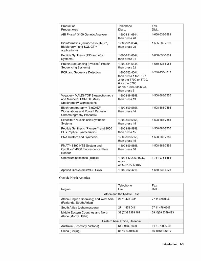
Product orProduct Area
TelephoneDial...
FaxDial...
ABI P
RISM
®
3700 DNA Analyzer 1-800-831-6844,then press
81-650-638-5981
DNA Synthesis 1-800-831-6844,then press
211-650-638-5981
Fluorescent DNA Sequencing 1-800-831-6844,then press
221-650-638-5981
Fluorescent Fragment Analysis (includes GeneScan
®
applications)1-800-831-6844,then press
231-650-638-5981
Integrated Thermal Cyclers (ABI P
RISM
®
877 and Catalyst 800 instruments)1-800-831-6844,then press
241-650-638-5981
Introduction 1-5
Outside North America
ABI P
RISM
®
3100 Genetic Analyzer 1-800-831-6844,then press
261-650-638-5981
BioInformatics (includes BioLIMS
™,
BioMerge
™
, and SQL GT
™
applications)
1-800-831-6844,then press
251-505-982-7690
Peptide Synthesis (433 and 43X Systems)
1-800-831-6844,then press
311-650-638-5981
Protein Sequencing (Procise
‚
Protein Sequencing Systems)
1-800-831-6844,then press
321-650-638-5981
PCR and Sequence Detection 1-800-762-4001,then press
1 for PCR,2 for the 7700 or 5700,6 for the 6700or dial 1-800-831-6844, then press 5
1-240-453-4613
Voyager
‰
MALDI-TOF Biospectrometry and Mariner
‰
ESI-TOF Mass Spectrometry Workstations
1-800-899-5858,then press
131-508-383-7855
Biochromatography (BioCAD
‚
Workstations and Poros
‚
Perfusion Chromatography Products)
1-800-899-5858,then press
141-508-383-7855
Expedite
‰
Nucleic acid Synthesis Systems
1-800-899-5858,then press
151-508-383-7855
Peptide Synthesis (Pioneer
‰
and 9050 Plus Peptide Synthesizers)
1-800-899-5858,then press
151-508-383-7855
PNA Custom and Synthesis 1-800-899-5858,then press
151-508-383-7855
FMAT‰ 8100 HTS System and Cytofluor‚ 4000 Fluorescence Plate Reader
1-800-899-5858,then press 16
1-508-383-7855
Chemiluminescence (Tropix) 1-800-542-2369 (U.S. only),or 1-781-271-0045
1-781-275-8581
Applied Biosystems/MDS Sciex 1-800-952-4716 1-650-638-6223
RegionTelephoneDial...
FaxDial...
Africa and the Middle East
Africa (English Speaking) and West Asia (Fairlands, South Africa)
27 11 478 0411 27 11 478 0349
South Africa (Johannesburg) 27 11 478 0411 27 11 478 0349
Middle Eastern Countries and North Africa (Monza, Italia)
39 (0)39 8389 481 39 (0)39 8389 493
Eastern Asia, China, Oceania
Australia (Scoresby, Victoria) 61 3 9730 8600 61 3 9730 8799
China (Beijing) 86 10 64106608 86 10 64106617
Product orProduct Area
TelephoneDial...
FaxDial...

1-6 Introduction
Hong Kong 852 2756 6928 852 2756 6968
Korea (Seoul) 82 2 593 6470/6471 82 2 593 6472
Malaysia (Petaling Jaya) 60 3 758 8268 60 3 754 9043
Singapore 65 896 2168 65 896 2147
Taiwan (Taipei Hsien) 886 2 22358 2838 886 2 2358 2839
Thailand (Bangkok) 66 2 719 6405 66 2 319 9788
Europe
Austria (Wien) 43 (0)1 867 35 75 0 43 (0)1 867 35 75 11
Belgium 32 (0)2 712 5555 32 (0)2 712 5516
Czech Republic and Slovakia (Praha) 420 2 61 222 164 420 2 61 222 168
Denmark (Naerum) 45 45 58 60 00 45 45 58 60 01
Finland (Espoo) 358 (0)9 251 24 250 358 (0)9 251 24 243
France (Paris) 33 (0)1 69 59 85 85 33 (0)1 69 59 85 00
Germany (Weiterstadt) 49 (0) 6150 101 0 49 (0) 6150 101 101
Hungary (Budapest) 36 (0)1 270 8398 36 (0)1 270 8288
Italy (Milano) 39 (0)39 83891 39 (0)39 838 9492
Norway (Oslo) 47 23 12 06 05 47 23 12 05 75
Poland, Lithuania, Latvia, and Estonia (Warszawa)
48 (22) 866 40 10 48 (22) 866 40 20
Portugal (Lisboa) 351 (0)22 605 33 14 351 (0)22 605 33 15
Russia (Moskva) 7 095 935 8888 7 095 564 8787
South East Europe (Zagreb, Croatia) 385 1 34 91 927 385 1 34 91 840
Spain (Tres Cantos) 34 (0)91 806 1210 34 (0)91 806 1206
Sweden (Stockholm) 46 (0)8 619 4400 46 (0)8 619 4401
Switzerland (Rotkreuz) 41 (0)41 799 7777 41 (0)41 790 0676
The Netherlands (Nieuwerkerk a/d IJssel)
31 (0)180 331400 31 (0)180 331409
United Kingdom (Warrington, Cheshire) 44 (0)1925 825650 44 (0)1925 282502
All other countries not listed(Warrington, UK)
44 (0)1925 282481 44 (0)1925 282509
Japan
Japan (Hacchobori, Chuo-Ku, Tokyo) 81 3 5566 6230 81 3 5566 6507
Latin America
Del.A. Obregon, Mexico 305-670-4350 305-670-4349
RegionTelephoneDial...
FaxDial...
Introduction 1-7
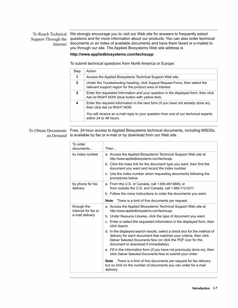
To Reach TechnicalSupport Through the
Internet
We strongly encourage you to visit our Web site for answers to frequently asked questions and for more information about our products. You can also order technical documents or an index of available documents and have them faxed or e-mailed to you through our site. The Applied Biosystems Web site address is
http://www.appliedbiosystems.com/techsupp
To Obtain Documentson Demand
Free, 24-hour access to Applied Biosystems technical documents, including MSDSs, is available by fax or e-mail or by download from our Web site.
To submit technical questions from North America or Europe:
Step Action
1 Access the Applied Biosystems Technical Support Web site.
2 Under the Troubleshooting heading, click Support Request Forms, then select the relevant support region for the product area of interest.
3 Enter the requested information and your question in the displayed form, then click Ask Us RIGHT NOW (blue button with yellow text).
4 Enter the required information in the next form (if you have not already done so), then click Ask Us RIGHT NOW.
You will receive an e-mail reply to your question from one of our technical experts within 24 to 48 hours.
To order documents... Then...
by index number a. Access the Applied Biosystems Technical Support Web site at http://www.appliedbiosystems.com/techsupp
b. Click the Index link for the document type you want, then find the document you want and record the index number.
c. Use the index number when requesting documents following the procedures below.
by phone for fax delivery
a. From the U.S. or Canada, call 1-800-487-6809, orfrom outside the U.S. and Canada, call 1-858-712-0317.
b. Follow the voice instructions to order the documents you want.
Note There is a limit of five documents per request.
through the Internet for fax or e-mail delivery
a. Access the Applied Biosystems Technical Support Web site at http://www.appliedbiosystems.com/techsupp
b. Under Resource Libraries, click the type of document you want.
c. Enter or select the requested information in the displayed form, then click Search.
d. In the displayed search results, select a check box for the method of delivery for each document that matches your criteria, then click Deliver Selected Documents Now (or click the PDF icon for the document to download it immediately).
e. Fill in the information form (if you have not previously done so), then click Deliver Selected Documents Now to submit your order.
Note There is a limit of five documents per request for fax delivery but no limit on the number of documents you can order for e-mail delivery.


Overview of Sequence Detection Software 2-1
Overview of Sequence Detection Software 2
Introduction
General The Sequence Detection application program allows you to set up sample and experimental information, and run the thermal cycler while measuring and analyzing fluorescence from your 96-well reaction plate. This section describes the salient features of the Sequence Detection application program.
Appendix C, “Sequence Detection Software Reference,” provides detailed descriptions of the Sequence Detection application program. Appendix D, “Theory of Operation,” presents more specific information about 5´ nuclease assays with TaqMan® PCR reagents.
In This Chapter The contents of the chapter are as follows:
Topic See Page
Overview of Sequence Detection Software 2-2
General 2-2
Software Control of the Instrument and the Experiment 2-3
Analyzed Data: The Terminology 2-3
Run Types and Plate Types 2-4
General Assumption 2-4
Run Types 2-4
Plate Types 2-4
Features of the Sequence Detection Plate Document 2-5
General 2-5
Setup View 2-5
Analysis View 2-6
Dye Layers 2-7
Sequence Detection Help 2-8
How to use 2-8
2

2-2 Overview of Sequence Detection Software
Overview of Sequence Detection Software
General The Sequence Detection software program runs on a Macintosh computer connected to the ABI PRISM® 7700 Sequence Detector by a serial communication cable, as shown in Figure 2-1:
Figure 2-1 Interconnection of the Sequence Detector and Macintosh
The application program manages all communication with the instrument to perform the following tasks during Real Time and End Point runs:
� Set up sample and experimental information
� Operate the thermal cycler
� Collect and analyze fluorescence data
� Display data in graphic charts
� Export data and print reports of the results
An experiment performed completely on the ABI PRISM 7700 Sequence Detector goes through three phases: Setup, Run, and Analysis:
a) Setup - defining experiment setup and Thermal Cycler conditions
b) Run - performing Thermal cycling with real-=time collection of fluorescent signal changes
c) Analysis - applying Multicomponenting algorithms to fluorescence data
IMPORTANT In the Plate Read run mode, PCR may occur on the 7700 or an external thermal cycler, but only end-point analysis is performed and the benefits of real-time analysis are foregone. As you read this manual, keep in mind that much of the material is intended to support use of the instrument in its Real Time run mode where the full instrument capabilities are used.
continued on next page
7700 Sequence Detector
Macintosh computer
Serial cable

Overview of Sequence Detection Software 2-3
Software Control ofthe Instrument and
the Experiment
On the monitor screen, the Sequence Detection application mimics the 96-well plate you use to perform your experiment. Use the application to record the dyes and samples in each well of the 96-well plate, the thermal cycler parameters you use during the experiment, and then start the sequence detector.
During the Polymerase Chain Reaction (PCR), use the application to examine changes in fluorescence after PCR is complete, analyze the fluorescence data and generate a Standard Curve. Finally, you can save the plate setup information and acquired data as an electronic record of your experiment.
Analyzed Data:The Terminology
Real Time Runs
In Appendix D, “Theory of Operation,” you can find a thorough description of the TaqMan fluorescent probe, its performance during PCR, and how the increase in fluorescence signal can be used to quantitate samples. Briefly, data analysis on the Sequence Detection application uses three terms to express results: Rn, DRn, and CT.
Rn, or the normalized reporter signal, represents the fluorescence signal of the reporter dye divided by the fluorescence signal of the passive reference dye. During PCR, Rn increases as amplicon copy number increases until the reaction approaches a plateau. When using the instrument in its Plate Read mode, the fluorescence signal is read at a single point in time after the completion of PCR rather than continuously during the course of PCR.
DRn represents the normalized reporter signal minus the baseline signal established in the first few cycles of PCR. Like Rn, DRn increases during PCR as amplicon copy number increases until the reaction approaches a plateau.
CT, or threshold cycle, represents the PCR cycle at which an increase in reporter fluorescence above a baseline signal can first be detected. The Sequence Detection software generates a Standard Curve of CT vs. (LogN) Starting Copy Number for all standards and then determines the starting copy number of unknowns by interpolation.
In a PCR system with 100% efficiency, the threshold cycle decreases by one cycle as the concentration of template doubles.
2-4 Overview of Sequence Detection Software
Run Types and Plate Types
GeneralAssumption
This manual assumes you have a basic understanding of the polymerase chain reaction (PCR) and some experience setting up PCR experiments.
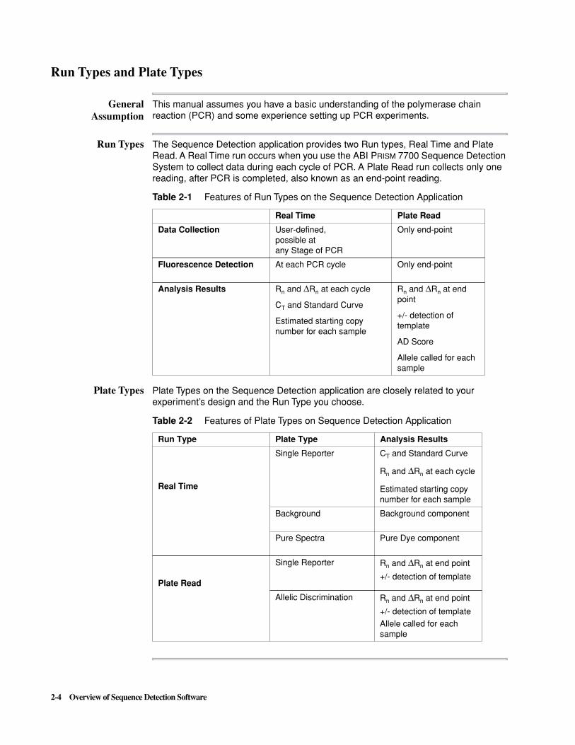
Run Types The Sequence Detection application provides two Run types, Real Time and Plate Read. A Real Time run occurs when you use the ABI PRISM 7700 Sequence Detection System to collect data during each cycle of PCR. A Plate Read run collects only one reading, after PCR is completed, also known as an end-point reading.
Plate Types Plate Types on the Sequence Detection application are closely related to your experiment’s design and the Run Type you choose.
Table 2-1 Features of Run Types on the Sequence Detection Application
Real Time Plate Read
Data Collection User-defined, possible at any Stage of PCR
Only end-point
Fluorescence Detection At each PCR cycle Only end-point
Analysis Results Rn and DRn at each cycle
CT and Standard Curve
Estimated starting copy number for each sample
Rn and DRn at end point
+/- detection of template
AD Score
Allele called for each sample
Table 2-2 Features of Plate Types on Sequence Detection Application
Run Type Plate Type Analysis Results
Real Time
Single Reporter CT and Standard Curve
Rn and DRn at each cycle
Estimated starting copy number for each sample
Background Background component
Pure Spectra Pure Dye component
Plate Read
Single Reporter Rn and DRn at end point
+/- detection of template
Allelic Discrimination Rn and DRn at end point
+/- detection of templateAllele called for each sample
Overview of Sequence Detection Software 2-5
Features of the Sequence Detection Plate Document
General The 96-well plate on the monitor screen has two views: Setup and Analysis. Each view contains tools for performing specific tasks. Both views have one or more “dye layers.” Each dye layer corresponds to the reporter dye on any probe.
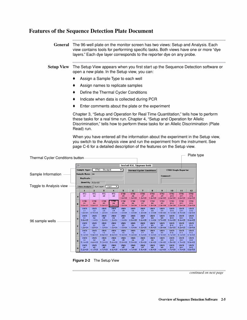
Setup View The Setup View appears when you first start up the Sequence Detection software or open a new plate. In the Setup view, you can:
� Assign a Sample Type to each well
� Assign names to replicate samples
� Define the Thermal Cycler Conditions
� Indicate when data is collected during PCR
� Enter comments about the plate or the experiment
Chapter 3, “Setup and Operation for Real Time Quantitation,” tells how to perform these tasks for a real time run. Chapter 4, “Setup and Operation for Allelic Discrimination,” tells how to perform these tasks for an Allelic Discrimination (Plate Read) run.
When you have entered all the information about the experiment in the Setup view, you switch to the Analysis view and run the experiment from the instrument. See page C-6 for a detailed description of the features on the Setup view.
Figure 2-2 The Setup View
continued on next page
Toggle to Analysis view
Thermal Cycler Conditions button
96 sample wells
Plate type
Sample Information

2-6 Overview of Sequence Detection Software
Analysis View In the Analysis view, you can:
� Start the Sequence Detector
� Collect fluorescence signals
� Analyze raw data, after all data is collected
Figure 2-3 The Analysis View
With Real Time run data, you can:
� Examine real-time changes in Rn and DRn at each PCR cycle
� Generate a Standard Curve
� View graphs of raw spectra for each cycle
� View graphs of Rn, DRn, and CT for each sample after analysis
� View multiple spectral components in each well
� Export tab-delimited data
With a Plate Read run, you can collect and analyze end-point data to calculate Rn and DRn for each sample after the final PCR cycle.
See page C-10 for a detailed description of the features of the Analysis view.
continued on next page
Overview of Sequence Detection Software 2-7
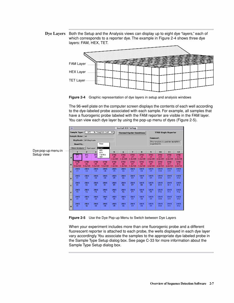
Dye Layers Both the Setup and the Analysis views can display up to eight dye “layers,” each of which corresponds to a reporter dye. The example in Figure 2-4 shows three dye layers: FAM, HEX, TET.
Figure 2-4 Graphic representation of dye layers in setup and analysis windows
The 96-well plate on the computer screen displays the contents of each well according to the dye-labeled probe associated with each sample. For example, all samples that have a fluorogenic probe labeled with the FAM reporter are visible in the FAM layer. You can view each dye layer by using the pop-up menu of dyes (Figure 2-5).
Figure 2-5 Use the Dye Pop-up Menu to Switch between Dye Layers
When your experiment includes more than one fluorogenic probe and a different fluorescent reporter is attached to each probe, the wells displayed in each dye layer vary accordingly. You associate the samples to the appropriate dye-labeled probe in the Sample Type Setup dialog box. See page C-33 for more information about the Sample Type Setup dialog box.
FAM Layer
TET Layer
HEX Layer
Dye pop-up menu in Setup view
2-8 Overview of Sequence Detection Software
Sequence Detection Help
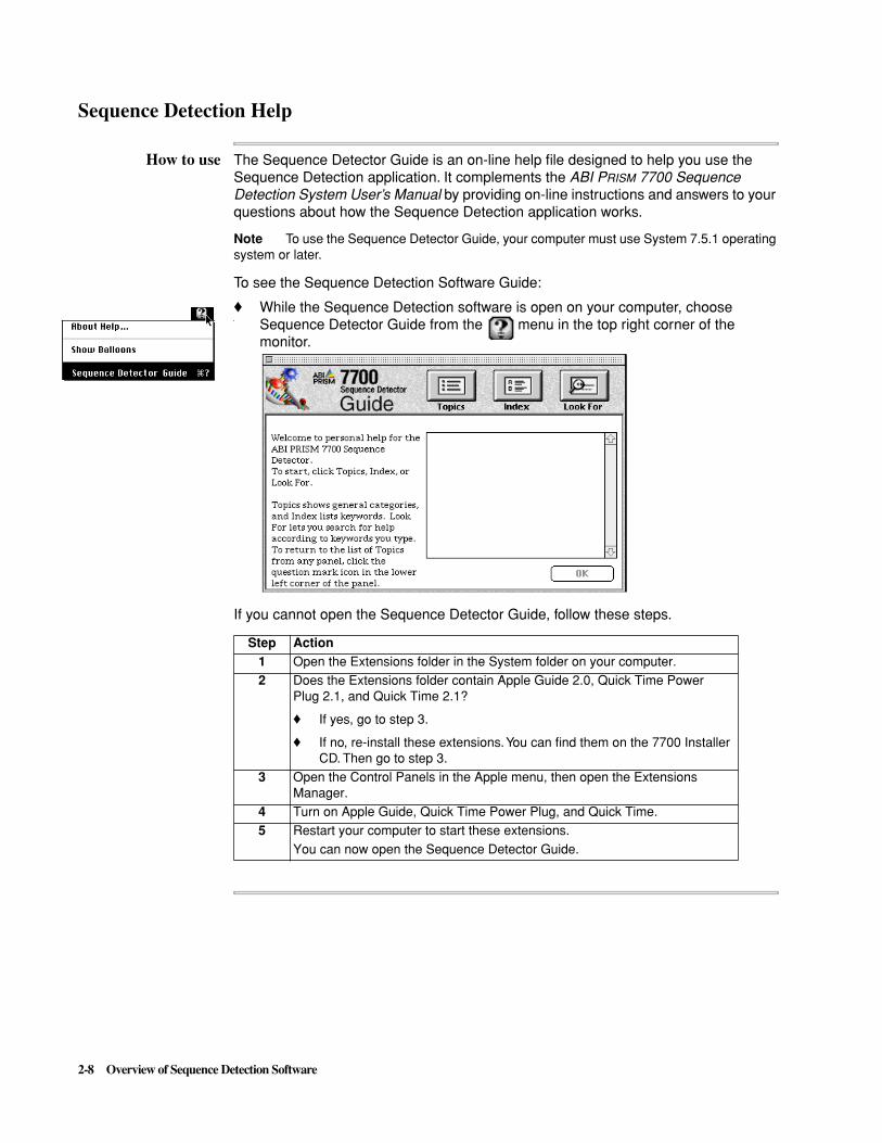
How to use The Sequence Detector Guide is an on-line help file designed to help you use the Sequence Detection application. It complements the ABI PRISM 7700 Sequence Detection System User’s Manual by providing on-line instructions and answers to your questions about how the Sequence Detection application works.
Note To use the Sequence Detector Guide, your computer must use System 7.5.1 operating system or later.
To see the Sequence Detection Software Guide:
� While the Sequence Detection software is open on your computer, choose Sequence Detector Guide from the menu in the top right corner of the monitor.
If you cannot open the Sequence Detector Guide, follow these steps.
Step Action1 Open the Extensions folder in the System folder on your computer.2 Does the Extensions folder contain Apple Guide 2.0, Quick Time Power
Plug 2.1, and Quick Time 2.1?
� If yes, go to step 3.
� If no, re-install these extensions. You can find them on the 7700 Installer CD. Then go to step 3.
3 Open the Control Panels in the Apple menu, then open the Extensions Manager.
4 Turn on Apple Guide, Quick Time Power Plug, and Quick Time.5 Restart your computer to start these extensions.
You can now open the Sequence Detector Guide.

Setup and Operation for Real Time Quantitation 3-1
Setup and Operation for Real Time Quantitation 3
Introduction
General This chapter describes how to use the Sequence Detection software to set up your experiment, run the Sequence Detector, and monitor PCR.
In This Chapter This chapter contains the following topics:
Topic See Page
Quick Review of Setup and Operation 3-2
Main Steps of Setup 3-3
Preparing for Sequence Detector Operation 3-4
Main Steps of Operation 3-4
Turning on Power to the Sequence Detector 3-4
General 3-5
Connecting the Application to the Instrument 3-5
Background Calibration 3-6
General 3-7
Generating a Background Component File 3-8
Pure Dye Spectra Calibration 3-9
General 3-10
Generating Pure Spectra Data 3-11
Extracting Component Pure Spectra 3-12
Selecting a Run Type and a Plate Type 3-13
General 3-14
Procedure 3-14
Assigning Sample Types to Plate Wells in the Setup View 3-14
General 3-15
Listing Sample Types 3-15
Procedure 3-16
Describing Sample Attributes 3-17
General 3-17
Procedures 3-17
Defining Thermal Cycler Conditions 3-19
Introduction 3-19
3

3-2 Setup and Operation for Real Time Quantitation
Viewing the Method 3-20
Viewing Data Collection 3-21
Entering Comments on the Setup View 3-22
Saving the Completed Setup 3-23
General 3-23
Procedure 3-23
Preparing for Sequence Detector Operation 3-24
General 3-24
Printing a 96-Well Sample Map 3-24
Preparing 96-Well Sample Trays for the Sequence Detector 3-25
Placing the 96-Well Sample Trays on the Sequence Detector 3-29
Closing the Cover on the Sample Block 3-30
Checking the Software Connection 3-30
Operating the Sequence Detector 3-31
General 3-31
Stopping the Sequence Detector 3-32
Opening the Cover after a Hold at 4°C 3-32
Topic See Page

Setup and Operation for Real Time Quantitation 3-3
Quick Review of Setup and Operation
Main Steps of Setup The table below provides you with a quick, graphic review of how to use the Sequence Detection software to set up and run your experiment on the Sequence Detector and monitor the reaction.
IMPORTANT During the installation of the ABI PRISM® 7700 Sequence Detector, data files for Background and Pure Dye Spectra are created in the Preferences folder. These files must be on your computer before you can set up an experiment with the Sequence Detection application program.
To set up the sequence detector, follow this procedure:
Step Action What it looks like... Do this...
1 Turning on power to the Sequence Detector
Turn on power at least 10 min. before starting a run.
See page 3-5.
2 Selecting a Run Type and a Plate Type
Choose New Plate in the File menu.
See page 3-13.
3 Designating dyes ChooseEdit Sample Listin the Sample Type pop-up menu
See page 3-14.
4 Assigning Sample Types to plate wells
Choose Sample Type Palette in the Setup menu.
See page 3-14.
5 Defining Thermal Cycler Conditions
Click the Thermal Cycler Conditions button on the Setup view.
See page 3-19.
Power switch

3-4 Setup and Operation for Real Time Quantitation
Preparing forSequence Detector
Operation
After you have set up and saved a plate document on the Sequence Detection software, load samples on the sample tray and place the sample tray in the sample block (see page 3-29).
IMPORTANT Always use MicroAmp® Optical Caps with either the MicroAmp® Optical 96-Well Reaction Plate or MicroAmp® Optical Tubes (in a tray/retainer) on the ABI PRISM 7700 Sequence Detector.
You can begin the Sequence Detector run after you tighten the sample block cover in place.
Main Steps ofOperation
The following table provides a quick review of how to operate the Sequence Detection software to acquire and save data.
To operate the Sequence Detector, follow this procedure:
6 Entering comments on the Setup view
Type in the Comments field.
See page 3-22.
7 Saving the completed setup
Choose Save As... in the File menu.See page 3-23.
Step Action What it looks like... Do this...
Step Action What it looks like... Do this...
1 Toggle to Analysis view
Click Show Analysis button in the Setup view.See page 3-31
2 Start Sequence Detector run
Click Run button in Analysis view.See page 3-31.
3 Monitor PCR progress
Thermal cycler status is shown in the Analysis View during a run.

Setup and Operation for Real Time Quantitation 3-5
Turning on Power to the Sequence Detector
General Turn on the power to the Sequence Detector at least ten minutes before using it to run a PCR experiment. When the power switch is in the off position, the cover to the sample block is not heated. When you turn on the power, the temperature of the sample block cover begins to rise. We do not recommend running the Sequence Detector until the temperature of the heated cover is approximately 105 °C.
Figure 3-1 Location of Power Switch on the ABI PRISM 7700 Sequence Detector
To turn on the power to the Sequence Detector, press the power switch to the On position, represented by a vertical line.
Connecting theApplication to the
Instrument
Two Things Required for Communication
To communicate between the Sequence Detector application program and the Sequence Detector, you need the following two things:
� A Macintosh serial cable used with the custom adapter (see page 2-2) between the computer and the instrument, and
� A software connection to establish communication, as described in "Procedure to Establish Communication" on page 3-6.
Stand-alone and Connected Modes
The Sequence Detection application program on the ABI PRISM® 7700 Sequence Detection System can be used in one of two modes: “stand-alone” or “connected” to the instrument.
� Stand-alone (when the application is not connected to the Sequence Detector) - use the application program to design PCR experiments or re-analyze previously collected data.
� Connected (when the application program is connected to the instrument) - use the software to design PCR experiments, run them on the instrument, then collect and analyze data.
Power switch
LED Display
IOn position
3-6 Setup and Operation for Real Time Quantitation
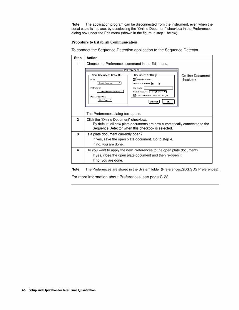
Note The application program can be disconnected from the instrument, even when the serial cable is in place, by deselecting the “Online Document” checkbox in the Preferences dialog box under the Edit menu (shown in the figure in step 1 below).
Procedure to Establish Communication
Note The Preferences are stored in the System folder (Preferences:SDS:SDS Preferences).
For more information about Preferences, see page C-22.
To connect the Sequence Detection application to the Sequence Detector:
Step Action
1 Choose the Preferences command in the Edit menu.
The Preferences dialog box opens.
2 Click the “Online Document” checkbox.By default, all new plate documents are now automatically connected to the Sequence Detector when this checkbox is selected.
3 Is a plate document currently open?If yes, save the open plate document. Go to step 4.If no, you are done.
4 Do you want to apply the new Preferences to the open plate document?If yes, close the open plate document and then re-open it.If no, you are done.
On-line Document checkbox

Setup and Operation for Real Time Quantitation 3-7
Background Calibration
General Spectra signals collected by the Sequence Detection application include signal inherent in the system or “background.” This background signal can interfere with the sensitivity of the Sequence Detection application and its ability to determine CT. To overcome this interference, you must generate a Background component file.
Generating aBackground
Component File
Requirements
Use TE Buffer or sterile, filtered water and the Background Plate Type to generate a Background data file. All wells on the Background Plate Type are automatically labeled “BKGND.”
Use the conditions specified in Table 3-1:
Procedure
Table 3-1 Thermal Cycling Conditions
Hold 1
Temperature (°C) 60.00
Time (min:sec) 2:00
To generate a background data file:
Step Action
1 In the File menu, choose New Plate.
The New Plate dialog box appears.
2 In the Plate Type pop-up, choose Background. The desired instrument, the 7700 Sequence Detector is the default choice.
Click OK to close the dialog box and open a Background plate document, like that shown below.
3-8 Setup and Operation for Real Time Quantitation
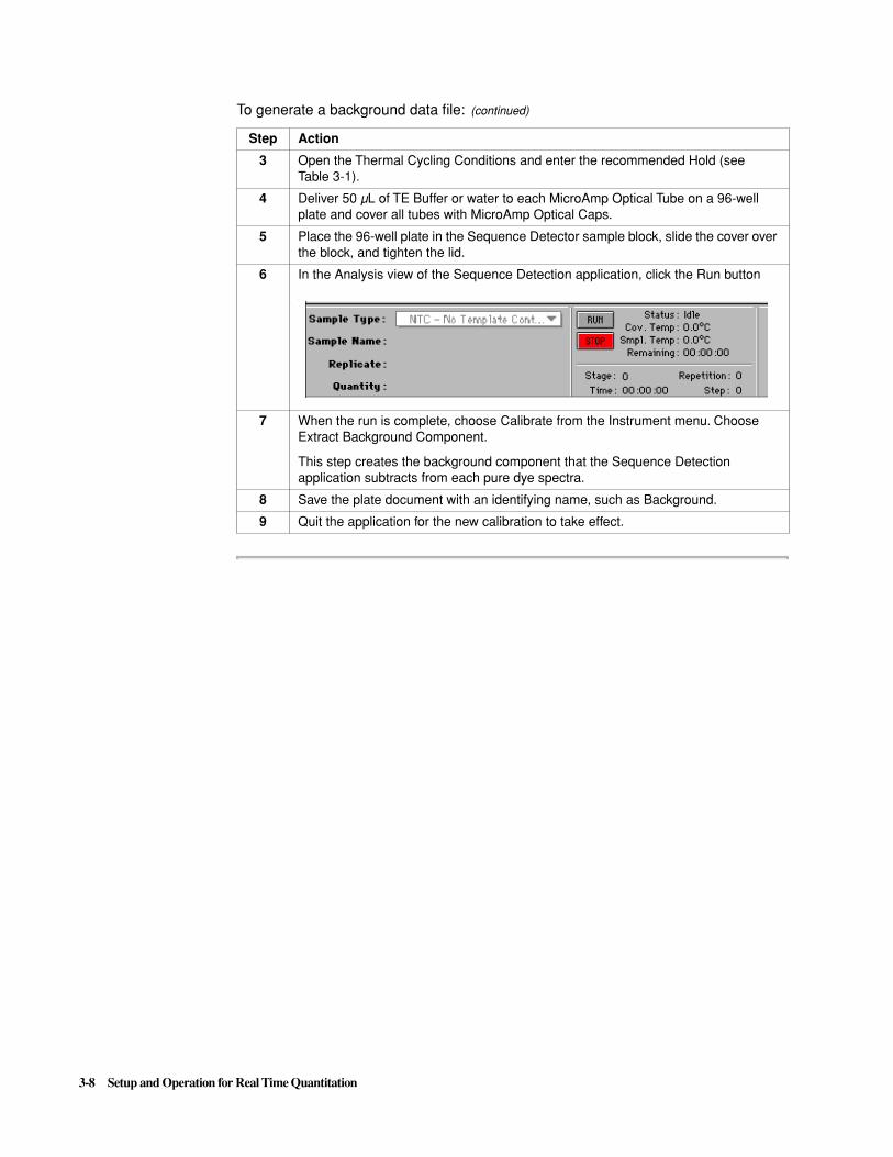
3 Open the Thermal Cycling Conditions and enter the recommended Hold (see Table 3-1).
4 Deliver 50 µL of TE Buffer or water to each MicroAmp Optical Tube on a 96-well plate and cover all tubes with MicroAmp Optical Caps.
5 Place the 96-well plate in the Sequence Detector sample block, slide the cover over the block, and tighten the lid.
6 In the Analysis view of the Sequence Detection application, click the Run button
.
7 When the run is complete, choose Calibrate from the Instrument menu. Choose Extract Background Component.
This step creates the background component that the Sequence Detection application subtracts from each pure dye spectra.
8 Save the plate document with an identifying name, such as Background.
9 Quit the application for the new calibration to take effect.
To generate a background data file: (continued)
Step Action

Setup and Operation for Real Time Quantitation 3-9
Pure Dye Spectra Calibration
General The Sequence Detection application features real-time monitoring of signal generated during PCR by fluorescent dyes FAM, TET, HEX, JOE, TAMRA, and ROX. Pure spectra information for these dye standards are collected during a 2-minute hold at 60 °C as part of the instrument installation procedure. The spectra data files are stored on the computer and used by the Sequence Detection application algorithm during data analysis. When a plate document is saved after data analysis, the pure spectra information is saved with the rest of the collected fluorescent data for that experiment.
Figure 3-2 Pure Spectra of Six Fluorescent Dyes
Figure 3-2 shows an example of the pure spectra for each of the dyes in the TaqMan Spectral Calibration Kit. The Y (vertical) axis represents spectral fluorescence normalized to an area of 1. You can view the Pure Spectra saved on your computer by choosing Edit Pure Spectra under the Calibrate command in the Instrument menu (see page C-40).
You can repeat the spectral calibration procedure to update the pure spectra data files or to test instrument performance. First, you must generate a Pure spectra data file, then extract each component dye spectrum from the collected data.
IMPORTANT You must generate a Background Component file before you can perform a Pure Dye Spectra Calibration.
continued on next page
FAM
TET HEX JOE TAMRA ROX
Nor
mal
ized
fluo
resc
ence
Wavelength (nm)

3-10 Setup and Operation for Real Time Quantitation
Generating PureSpectra Data
Requirements
Use the TaqMan Spectral Calibration Kit (P/N 401930), which contains six dye standards: FAM, TET, HEX, JOE, TAMRA, and ROX.
Use the conditions specified in Table 3-2:
Procedure
To generate a spectra data file:
continued on next page
Table 3-2 Thermal Cycling ConditionsHold 1
Temperature (°C) 60.00
Time (min:sec) 2:00
Step Action
1 In the File menu, choose New Plate.
The New Plate dialog box appears.
2 In the Plate Type pop-up menu, choose Pure Spectra. The desired instrument (7700 Sequence Detector) and Run type (Real Time) are the default choices.
Click OK to close the dialog box and open a Pure Spectra plate document.
3 Enter the Thermal Cycling Conditions shown above (Table 3-2).
4 On the plate document, designate four wells for each of the dye standards: FAM, TET, HEX, JOE, TAMRA, and ROX (using the plate setup shown in step 1 of the procedure on the next page for Extracting Spectra).
5 Deliver 50 µL of each dye standard to four MicroAmp Optical Tubes apiece on a 96-well plate. Use the same order designated on the Setup view of the Pure Spectra plate. Cover all tubes with MicroAmp Optical Caps.
6 Place the 96-well plate in the Sequence Detector sample block and tightly close the lid.
7 In the Analysis view of the Sequence Detector application, click the Run button.
When the run is finished, you can look at the raw spectra by double-clicking on any well in the Analysis view.
8 When the run is complete, save the plate document and data with an identifying name, such as Pure Spectra.
After you generate the pure spectra data, continue by calibrating each component dye (using the Extraction procedure on the next page).

Setup and Operation for Real Time Quantitation 3-11
ExtractingComponent Pure
Spectra
Use the Analysis view of the Sequence Detection application to extract each pure dye spectrum from the collected Pure spectra data file. You must extract dye spectra for the reporter dye on each TaqMan probe (FAM, JOE, HEX or TET), the quencher on each TaqMan probe (TAMRA), and the passive reference (ROX).
To extract component pure spectra:
Step Action
1 In the Analysis view, select the first set of wells that contain the same dye (FAM in our example).
2 In the Instrument menu, choose Calibrate, then choose Extract Spectra Component and Pure Spectra, or use the keyboard shortcut, c J.
The Pure Spectra Extraction dialog box appears.
The dye name attached to the selected wells appears in the field labeled “Pure Spectra Name.” You can edit this dye name.
You can also change the color assigned to the Pure Spectra by double-clicking the color and using the Color Wheel dialog box (page C-35).
3 Click OK to close the Pure Spectra Extraction dialog box.
The Extract Pure Spectra dialog box opens and displays a graph of the dye spectra for each selected well. Background component has been subtracted from the spectra on the display and each spectra has been normalized to an area of 1.

3-12 Setup and Operation for Real Time Quantitation
4 Click the boxes in the scroll box labeled “Sample (Well)” to turn off and on each well’s spectra in the graph.
5 Below the graph, you can select and discard wells that contain spectra you want to eliminate from the pure dye spectra.
As a general rule, discard spectra that have shapes that do not fit the shape of the other spectra. Differences in spectra amplitude are not significant if the shape is a good fit.
6 If you want to save the dialog box with your changes, click OK.
If you want to close the dialog box without saving your changes or any of the dye spectra, click Cancel.
7 Return to step 1 and repeat this procedure for each dye you need to extract.
8 When all dyes have been extracted, quit the application for the new calibration to take effect.
To extract component pure spectra: (continued)
Step Action
Spectra

Setup and Operation for Real Time Quantitation 3-13
Selecting a Run Type and a Plate Type
General When you first start the Sequence Detection application, a new plate document appears on the monitor screen. By default, the new plate document uses the Single Reporter Plate Type. In the Preferences dialog box, you can change the default Run Type and Plate Type. See page C-22 for a description of Preferences.
Choose a Run Type and a Plate Type that supports your experiment’s design and function. Choices available include
� Single Reporter Real Time or Plate Read plates
� Allelic Discrimination (AD) plate
See page 2-4 for more information on Run Types and Plate Types.
IMPORTANT During the installation of the ABI PRISM 7700 Sequence Detector, data files for both Background and Pure Dye Spectra are created by the computer. These files must be on your computer before you can set up an experiment with the Sequence Detection software. See page 3-7 and page 3-10 for information on creating these files.
You can also use the New Plate dialog box to override the Preferences and choose another Plate Type.
Procedure To use the New Plate dialog box:
Step Action
1 If a plate document is already open, close it.
2 Choose New Plate in the File menu.
The New Plate dialog box opens.
3 Select a Plate Type in the Plate Type menu (the 7700 Sequence Detector is chosen as a default).
4 In the Run pop-up menu, select the appropriate Run Type.
5 Click OK to close the dialog box and open a new plate document.
The new plate document assumes the characteristics of the selected Run and Plate Types.
3-14 Setup and Operation for Real Time Quantitation
Assigning Sample Types to Plate Wells in the Setup View
General For real-time fluorescence monitoring and data analysis, each well in the Setup view must contain accurate sample type information.
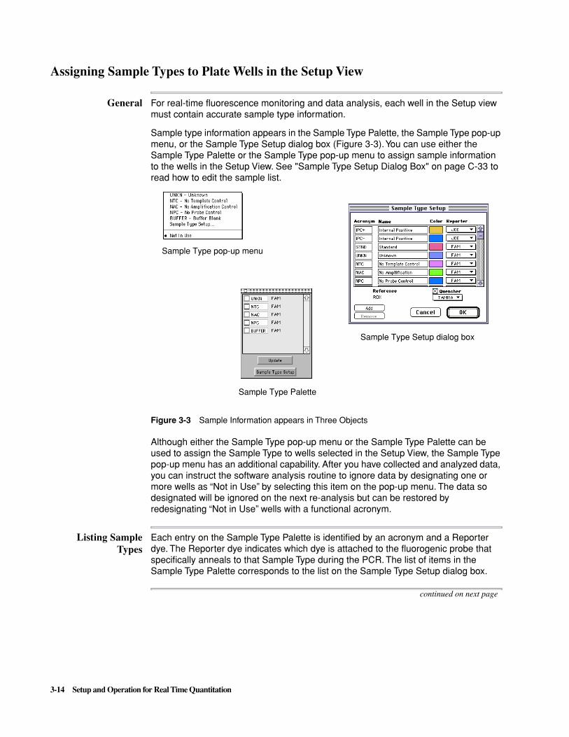
Sample type information appears in the Sample Type Palette, the Sample Type pop-up menu, or the Sample Type Setup dialog box (Figure 3-3). You can use either the Sample Type Palette or the Sample Type pop-up menu to assign sample information to the wells in the Setup View. See "Sample Type Setup Dialog Box" on page C-33 to read how to edit the sample list.
Figure 3-3 Sample Information appears in Three Objects
Although either the Sample Type pop-up menu or the Sample Type Palette can be used to assign the Sample Type to wells selected in the Setup View, the Sample Type pop-up menu has an additional capability. After you have collected and analyzed data, you can instruct the software analysis routine to ignore data by designating one or more wells as “Not in Use” by selecting this item on the pop-up menu. The data so designated will be ignored on the next re-analysis but can be restored by redesignating “Not in Use” wells with a functional acronym.
Listing SampleTypes
Each entry on the Sample Type Palette is identified by an acronym and a Reporter dye. The Reporter dye indicates which dye is attached to the fluorogenic probe that specifically anneals to that Sample Type during the PCR. The list of items in the Sample Type Palette corresponds to the list on the Sample Type Setup dialog box.
continued on next page
Sample Type Palette
Sample Type pop-up menu
Sample Type Setup dialog box

Setup and Operation for Real Time Quantitation 3-15
Procedure The procedure below is used to assign sample types in the Setup View.
To assign a sample to one or more wells with the Sample type Palette:
Step Action
1 Choose Sample Type Palette in the Setup menu.
2 Compare the entries in the Sample Type Palette to the samples you are using in your experiment. Make sure each Sample Type has the right Reporter Dye assigned to it.
If the palette contains all the Sample types you need and they each have the appropriate Reporter Dye, you can now assign the Sample Types to the wells in the Plate window.
If you need to edit an entry in the Sample Type Palette, use the Sample Type Setup dialog box. See "Sample Type Setup Dialog Box" on page C-33.
3 Click a well on the Setup view to select it.
A selected well is outlined in black.
� Click and drag across the plate to select multiple contiguous wells.
� Press the Command (c)key and click on wells to select multiple discontinuous wells.Click on a row or column label (A–H, 1–12) to select an entire row or column of wells.
Sample type Reporter dye
Use to edit Sample List
Update button
Selected well

3-16 Setup and Operation for Real Time Quantitation
4 In the Sample Type Palette, click the check box next to the acronym for the sample you want to put in the selected well(s).
If the Sample Type Palette does not contain all the samples you need, see "Sample Type Setup Dialog Box" on page C-33.
Note To generate a Standard Curve with the Sequence Detection software, use at least 5 standards or samples of known template amount. The range of known copy numbers should bracket the anticipated copy numbers of the unknown samples on the same plate.
5 Click the Update button on the Sample Type Palette to assign the sample to the selected well.
The selected well now displays the acronym for the sample you’ve selected. If you have added more than one sample+probe system, use the dye pop-up menu to look at each dye layer. (See "Dye Layers" on page 2-7.)
Note Use at least five Standards to generate a Standard curve.
To assign a sample to one or more wells with the Sample type Palette: (continued)
Step Action
Setup and Operation for Real Time Quantitation 3-17
Describing Sample Attributes
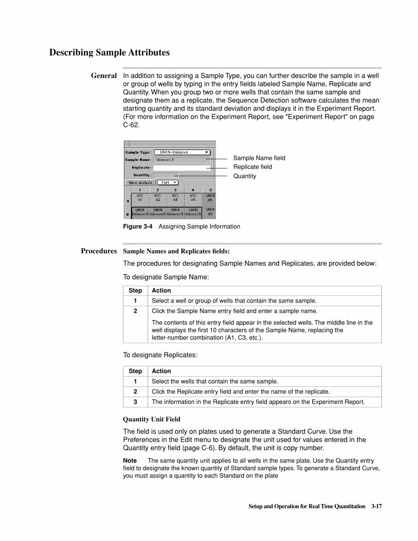
General In addition to assigning a Sample Type, you can further describe the sample in a well or group of wells by typing in the entry fields labeled Sample Name, Replicate and Quantity. When you group two or more wells that contain the same sample and designate them as a replicate, the Sequence Detection software calculates the mean starting quantity and its standard deviation and displays it in the Experiment Report. (For more information on the Experiment Report, see "Experiment Report" on page C-62.
Figure 3-4 Assigning Sample Information
Procedures Sample Names and Replicates fields:
The procedures for designating Sample Names and Replicates, are provided below:
To designate Replicates:
Quantity Unit Field
The field is used only on plates used to generate a Standard Curve. Use the Preferences in the Edit menu to designate the unit used for values entered in the Quantity entry field (page C-6). By default, the unit is copy number.
Note The same quantity unit applies to all wells in the same plate. Use the Quantity entry field to designate the known quantity of Standard sample types. To generate a Standard Curve, you must assign a quantity to each Standard on the plate
Sample Name fieldReplicate field
Quantity
To designate Sample Name:
Step Action
1 Select a well or group of wells that contain the same sample.
2 Click the Sample Name entry field and enter a sample name.
The contents of this entry field appear in the selected wells. The middle line in the well displays the first 10 characters of the Sample Name, replacing the letter-number combination (A1, C3, etc.).
Step Action
1 Select the wells that contain the same sample.
2 Click the Replicate entry field and enter the name of the replicate.
3 The information in the Replicate entry field appears on the Experiment Report.

3-18 Setup and Operation for Real Time Quantitation
To designate sample quantity:
IMPORTANT .
If you know that Standard 1 has a copy number of approximately 1000, use copy number as the quantity unit for all standards. All results for Unknowns are expressed in the same quantity unit as the Standards.
Step Action
1 Select wells that contain the same concentration or copy number of template.
2 Click the Quantity entry field and enter a number. Do not use commas to separate integers.
3 Press the Tab key.
The number you enter is automatically converted to scientific notation. (See "Entry Fields" on page C-6 for an explanation of scientific notation).

Setup and Operation for Real Time Quantitation 3-19
Defining Thermal Cycler Conditions
Introduction The Thermal Cycler Conditions dialog box contains two views. Use the first view (the Time and Temperature view) to define the thermal cycler method plus the Sample Volume. Use the second view (the Data Collection view) to indicate where you want the Sequence Detection software to collect data during the PCR run.
To open the Thermal Cycler Conditions dialog box, click the Thermal Cycler Conditions button on the Setup view. The dialog box will open in the first view shown below:
Figure 3-5 Two Thermal Cycler Conditions Views
Define data collection in this view (Data Collect View)
Buttons to togglebetween views
Number of cyclerepetitions
Ramp
Temperature
Time
Define thermal cycler method in this view (Time and Temperature view)

3-20 Setup and Operation for Real Time Quantitation
:
Viewing the Method Graphic Representation of a Method
The upper illustration in Figure 3-5 provides a graphic representation of a method. A method contains all the information about time and temperature changes that occur during a complete sequence detector run.
There are several ways to edit the features in a method. You can:
� Add or remove Steps, Cycles, or Holds
� Change the temperature or time associated with any Step
� Adjust the ramp time between two Steps
� Define an Auto Increment for time and temperature
IMPORTANT Do not enter a value less than 30 seconds (00:30) for an extension step in a Cycle. See page C-30 for more information on extension time.
See "Setting Up Thermal Cycler Conditions" on page C-24 for more information on thermal cycler setup.
Designating Sample Volume
In the Thermal Cycler Conditions dialog box, you can indicate the volume of sample in each well on the 96-well plate. Sample, in this case, refers to the entire contents of any well, including buffer blank, or any combination of master mix and nucleic acids. The default sample volume, 50 µL, can be modified in the Preferences dialog box (see page C-22).
Note All wells on one plate should contain the same volume of sample. Performance specifications on the ABI PRISM 7700 are based on 50 µL of sample in each well.
Ramp Times
The ramp time between two Steps in the Thermal Cycler Conditions is the time needed to go from one temperature to the next. When the ramp time is set to the minimum ramp time of zero, the rate of temperature change on the thermal cycler is approximately 1 °C/second. For example, the shortest possible time necessary to ramp from 50 °C to 95 °C is approximately 45 seconds. The maximum ramp time is 9 minutes and 59 seconds. See page C-29 for information on changing ramp times.
Auto Increment and Decrement
The Auto Increment feature appears in the Thermal Cycler Conditions dialog box. With this feature, you can automatically increase or decrease the time or temperature associated with any Step by a fixed amount with each Cycle repetition. For example, you can increase the extension time of a Cycle to accommodate the increased amount of amplicons produced as PCR progresses.
To change views in the Thermal Cycler Conditions dialog box:
Step Action
1 Click the button labeled “Show Data Collection” to define data collection.
2 Click the button labeled “Show Time and Temp” to define the method.

Setup and Operation for Real Time Quantitation 3-21
IMPORTANT The temperature range of the thermal cycler sample block is 4.0 to 99.9 °C. The Sequence Detection software does not accept an auto-increment value that would eventually cause the temperature of the sample block to exceed this range.
See page C-30 for more information on the Auto Increment feature.
Viewing DataCollection
The Data Collect view, shown below, displays the same method you created in the Time and Temperature view. You must put a Data Collection icon on this method wherever you want the Sequence Detection software to collect data during a run. For meaningful real-time data analysis, there must be a Data Collection icon on the extension step.
Figure 3-6 Using a Data Collect Icon
To add or remove a Data Collection icon:
� Click once on a plateau in the Data Collection view to add an icon.
� Click once on a Data Collection icon to remove the icon.
See Data Collection on page C-31 for more details about data collection during a run.
See "Instrument Menu" on page C-40 for information on how collected data is analyzed.
Note The 7700 Sequence Detector does not collect data on temperature ramps.
Data Collection icon

3-22 Setup and Operation for Real Time Quantitation
Entering Comments on the Setup View
You can attach notes or comments about the experiment in the Comment entry field, in the top right corner of the Setup view. The comments entered in the Setup view also appear in the Comments field of the Analysis view and the Experiment Report.
Figure 3-7 Comments on Setup View appear in Experiment Report
� To enter comments in the Setup view, click the cursor in the Comments entry field and type your comments.
The comments field may contain up to 255 characters.
You can modify comments on the Setup view, but not on the Analysis view or the Experiment Report.
Experiment Report
Setup View

Setup and Operation for Real Time Quantitation 3-23
Saving the Completed Setup\
General You can save the Setup using a unique, descriptive name. This name appears on the Experiment Report as the File Name.
You can also choose to save the Setup as a normal file or as a stationery file. A normal file saves all information on the plate document, including acquired data, but not analyzed data. Changes you make to a normal file remain in the file.
The stationery file saves the following user-defined information and is used as a template for experiments that you plan to repeat frequently:
� Run Type and Plate Type
� Sample Types in each well
� Thermal Cycler Conditions
When you open a stationery file, Sequence Detection software opens a copy of the file for you to use. Changes you make to the copy do not affect the original stationery plate file. When you save or close the copy, you can save it as a normal file or re-name it as another stationery file. The Sequence Detection software labels stationery plate files with a unique icon.
Procedure To save the Setup:
Step Action
1 Choose Save in the File menu and enter a descriptive name in the directory dialog box.
2 Click a format icon.
� Choose the Stationery format icon to create a stationery file.
� Choose the Normal format icon to create a normal file.
Stationery format icon
Normal format icon

3-24 Setup and Operation for Real Time Quantitation
Preparing for Sequence Detector Operation
General Once you have set up your experiment on the Setup view, you can print a map of the 96-well plate with the samples listed in each well. Refer to the sample map to distribute your samples on the 96-well sample tray. (Also, see Appendix B, Purification of DNA.)
Printing a 96-WellSample Map
A sample map shows how samples and standards are distributed. You can print this map for your paper records and to help you set up your experiment. The full-sized, rectangular map is wider than 8.5 inches. Use the Page Setup dialog box to determine the size and orientation of the printed sample map.
Figure 3-8 A reduced view of a sample map
To print a 96-well sample map:
continued on next page
Step Action
1 With the Setup view displayed on your computer monitor, choose Page Setup in the File menu.
2 The Page Setup dialog box appears.
3 Click the Landscape orientation icon. You can also reduce the map in the Reduce or Enlarge entry field. Click OK to close the Page Setup dialog box.
4 Choose Print from the File menu. Click the Print button to print.
Landscape orientation

Setup and Operation for Real Time Quantitation 3-25
Preparing 96-WellSample Trays for the
Sequence Detector
Two 96-Well Plate Formats
A 96-well plate can be comprised of either a MicroAmp Optical 96-Well Reaction Plate and MicroAmp Optical Caps, as shown in Figure 3-9, or of individual MicroAmp Optical Tubes placed in a MicroAmp 9600 tray and then capped with MicroAmp Optical Caps as shown in Figure 3-10.
The Sequence Detector sample block accommodates a 96-well plate with MicroAmp Optical Caps, in either format. Use a 96-well plate, in one of these formats to set up your experiment. Remove the base before placing the 96-well plate in the Sequence Detector sample block.
Figure 3-9 Assembly of MicroAmp® Optical 96-Well Reaction Plate and MicroAmp® Optical Caps on Optical Support Base
Optical Support Base(006899)
MicroAmp Optical 96-Well Reaction Plate(N801-0560)
MicroAmp Optical Caps(N801-0935)
45° corner of 96-well plate at position A12

3-26 Setup and Operation for Real Time Quantitation
Figure 3-10 Assembly of Sample Tray, Optical Tubes and Caps on Optical Support Base
IMPORTANT Remove the Optical Support base before placing the tray on the sample block.
The 96-well plate and optical caps have been especially designed to work with the system of fiber optics and CCD (charged-couple device) camera that monitors fluorescence during PCR.
IMPORTANT For accurate fluorescence detection, always use the MicroAmp 96-well plate and Optical Caps on the ABI PRISM 7700 Sequence Detector. Do not attach sticky labels to the tubes or caps or mark them with ink.
The design of the MicroAmp Optical Cap incorporates a thin-walled optically clear dome that allows transmission of fluorescent signals.
IMPORTANT Use the MicroAmp® Cap-installing Tool (N801-0438) to securely tighten the MicroAmp® Optical Caps onto the MicroAmp® Optical Tubes.
Optical Support Base(006899)NOT the 9600 MicroAmp base(N801-0531)
MicroAmp 9600 Tray(N801-0530)
MicroAmp 9600 Tray retainer(N801-0530)
MicroAmp Optical Tubes(N801-0933)
MicroAmp Optical Caps(N801-0935)
Position A1
Fits over protrusion on sample block

Setup and Operation for Real Time Quantitation 3-27
Procedure
To prepare your 96-well plate for analysis:
Step Action
1 � If you are using the 96-well reaction plate, place the plate on the Optical Support support base as shown in Figure 3-11.
� If you are using the assembly shown in Figure 3-10, assemble the components as shown in the figure and place the assembly on the Optical Support Base as shown in Figure 3-11.
2 Add the samples for your experiment to wells as indicated on your printed sample map.
3 Hold a strip of MicroAmp Optical Caps over a row of tubes and use the blunt end of the cap installing tool to push and seat each cap firmly in place (Figure 3-11).
Figure 3-11 Pushing the Caps in Place with the MicroAmp® Cap-installing Tool (N801-0438)

3-28 Setup and Operation for Real Time Quantitation
continued on next page
4 After all the caps are in place, with moderate force, use the roller end of the tool to roll over all caps (Figure 3-12).
Figure 3-12 Reinforcing Cap Placements with the Roller End
To prepare your 96-well plate for analysis: (continued)
Step Action

Setup and Operation for Real Time Quantitation 3-29
Placing the 96-WellSample Trays on the
Sequence Detector
� Place the 96-well sample tray on the Sample Detector Sample Block as shown in Figure 3-13.
The 96-well sample tray fits on the sample block in only one position. An opening on the left side of the tray fits onto a protrusion on the surface of the sample block. When the tray has been correctly placed in the sample block, the A1 position on the sample tray sits in the upper left-hand corner of the sample block (Figure 3-13).
CAUTION The Sequence Detector does not operate properly when the sample tray is improperly positioned on the sample block.
Figure 3-13 Placing a 96-Well Tray on the Sequence Detector Sample Block
CAUTION DO NOT analyze radioactive samples on the ABI PRISM 7700 Sequence Detector. If radioactivity leaks onto the sample block, the entire block must be removed for a lengthy decontamination process. This decontamination process is not covered by the instrument’s Limited Warranty.
Note The upper right-hand corner of a 96-well plate (near A-12) is usually indicated with a triangular cut. This is the industry standard indicator for the proper orientation of a 96-well plate.
continued on next page
Position A1
Position A12

3-30 Setup and Operation for Real Time Quantitation
Closing the Cover onthe Sample Block
After the 96-well plate is in place, do the following:
When the cover is properly tightened, the white area of the ring on top of the large knob faces the front of the instrument.
Figure 3-14 Tighten the Knob on the Sample Block Cover
Checking theSoftware Connection
When you are ready to run the Sequence Detector, check that the Sequence Detection application is connected to the instrument.
To check the connection to the Sequence Detector:
Step Action
1 Slide the sample block cover back over the sample block.
2 Turn the large knob on top of the cover clockwise to tighten the lid in place, referring to Figure 3-14.
White area on knob faces front when properly tightened.
Step Action
1 Click the Show Analysis button to toggle the plate document to the Analysis view.
2 Verify that the Status field displays the word “Idle.”
If the Status field displays the word “Offline,” the application is not connected to the instrument (see page 3-6).

Setup and Operation for Real Time Quantitation 3-31
Operating the Sequence Detector
General After all the sample wells are labeled on the Setup view, the sample tray has been placed in the sample block and the sample block cover tightly closed, you are ready to perform the PCR. Use the Analysis view to run the Sequence Detector and monitor thermal cycler status. The view button just above the wells in the Plate window lets you toggle between the Setup and Analysis views.
Figure 3-15 Two Plate Document Views
To run the Sequence Detector:
Show Analysis button
Run button
Setup view
Analysis view
Ready
Step Action
1 Click the Show Analysis button to toggle to the Analysis view.
2 Click the button labeled “Run” at the top of the Analysis view.
As the Sequence Detector begins to run, the Status field displays the word Waiting and the LED display light labelled “Comm” blinks green as the run information is transferred from the computer to the Sequence Detector.
3-32 Setup and Operation for Real Time Quantitation
IMPORTANT If the Status display reads “Offline”, the Sequence Detection application is not connected to the Sequence Detector and the run information cannot be transferred from the computer. See page 3-6 for how to connect the application to the instrument.
After the run begins, the Status fields display thermal cycler temperatures and run progress in the space under the Run button. See page C-12 for details on the Status values.
IMPORTANT If a power failure occurs during a run, fluorescence data collected before the power failure will be saved. After power is restored, you can recover the saved data by importing the temporary file saved in the “Spooled Items” folder within the SDS Preferences folder (System folder).
Stopping theSequence Detector
To stop the sequence detector during a run:
� Click the Stop button on the Analysis view at any time during PCR.
If you click the Stop button before the run is complete, a dialog box opens and asks if you want to save the collected data. See page C-11 for more information on saving collected data.
When you click the Stop button, a shutter closes to block out the laser signal, the temperature of the sample block begins to return to 25 C, and the cover interlocks are defeated so that you can the open the sequence detector cover.
! WARNING ! EXTREMELY HOT SURFACES. The temperature of the sample block cover may be as high as 105 °C. Avoid touching the sample block or the heated cover.
CAUTION DO NOT perform manual hot starts on the ABI PRISM 7700 Sequence Detector. Manual hot starts can cause random splashes of fluorescence-laden solution onto the sample block. This contamination interferes with the performance of the fiber optic system and can cause erroneous results. Always keep the wells on the 96-well plate tightly capped while they are on the sample block and throughout PCR.
Opening the Coverafter a Hold at 4°C
After a long Hold at 4 °C, the MicroAmp® Optical Caps may stick to the cover of the sample block, making it difficult to slide the cover back. To avoid this problem, stop the run and wait about 5 min until the temperature of the sample block returns to 25 °C before attempting to open the sample block cover.
An additional solution is to gently screw down the knob a little further, then release completely and slide the cover back.
CAUTION Opening the heated cover after starting a run defeats the cover interlocks, closes the shutters, and no fluorescence data will be collected.

Setup and Operation for Allelic Discrimination 4-1
Setup and Operation for Allelic Discrimination 4
Introduction
Overview The TaqMan® Allelic Discrimination Demonstration Kit shows how to use the ABI PRISM® 7700 Sequence Detection System to discriminate between the two alleles provided in the kit. Besides the two allele standards, the kit consists of heterozygous control DNA and a pre-made master mix of reagent intended for both robust chemistry and ease of use. The kit contains sufficient reagents to perform 200 reactions.
Allele 1 and Allele 2 Allele 1 and Allele 2 probes supplied in the Reagent Master Mix can be used with the specific Genomic Control DNA included in the kit. Custom probes must be designed for detection of any other templates. The design of these probes should follow the “Guidelines for the Design of Allelic Discrimination Primers and Probes” on page 15 of the TaqMan® Allelic Discrimination Kit Protocol.
Purpose of ThisChapter
This chapter uses the TaqMan Allelic Discrimination Demonstration Kit as a model of how to perform allelic discrimination on the ABI PRISM 7700 Sequence Detection System. When this kit is used on the ABI PRISM 7700 instrument, direct detection of PCR product is accomplished with no downstream processing. This method permits the analysis of thousands of samples per day with high sample-to-sample reproducibility. The example provided here demonstrates the software capabilities of the instrument while also providing a practical example of how to perform an allelic discrimination assay on the instrument.
In This Chapter This chapter contains the following topics:
Topic See Page
Running an Allelic Discrimination Assay 4-2
Setting Up a Plate 4-2
Run a Two-probe AD Assay 4-3
Analyzing the Data 4-4
Reading a Plate 4-4
Analyzing a Plate 4-4
Listing of Allelic Discrimination View Features 4-6
Mathematical Transformations 4-8
Overview 4-8
List of Mathematical Transformations 4-8
4

4-2 Setup and Operation for Allelic Discrimination
Running an Allelic Discrimination Assay
Setting Up a Plate When running an allelic discrimination (AD) assay, set up a plate as described below. Later, you can adapt the procedure to set up a plate template for your own assay:
Making Manual Calls 4-9
Background 4-9
Procedure 4-10
Topic See Page
To set up an allelic discrimination assay, follow this procedure:
Step Action
1 Choose New Plate in the File menu and then select the Allelic Discrimination plate type. Click Ok to open a new plate document.
Note This procedure assumes Preferences were set for the 7700. If Preferences have not been set, select the 7700 as the Instrument Type.
2 Assign sample types to the wells as shown in the example below. Later, when you are developing your own allelic discrimination assay, you can modify the Sample Type assignments.
NTC to wells A1 through A8
Allele 2 standard to wells B5 through B12
Allele 1 standard to wellsA9 through B4
UNKN assigned to remainder of B5 through B12wells
Allelic Plate assignments for the current example are as listed below:

Setup and Operation for Allelic Discrimination 4-3
Run a Two-probeAD Assay
See the TaqMan Allelic Discrimination Demonstration Kit Protocol (P/N 402875) for instructions on performing a two-probe allelic discrimination assay.
3 a. Use the Page Setup command to bring up the dialog box shown below:
b. Set up printing for the plate and Experiment Report by choosing the “Landscape” orientation (the second orientation in the figure) and by setting the percentage of the print to 95%.
c. Click OK to set up the plate with your settings.
4 To aid you in placing standards and samples in the 96-Well plate, print a copy of the plate setup using the Print command. This copy can be used as a “sample map” to aid you in loading the 96-Well plate.
To set up an allelic discrimination assay, follow this procedure: (continued)
Step Action
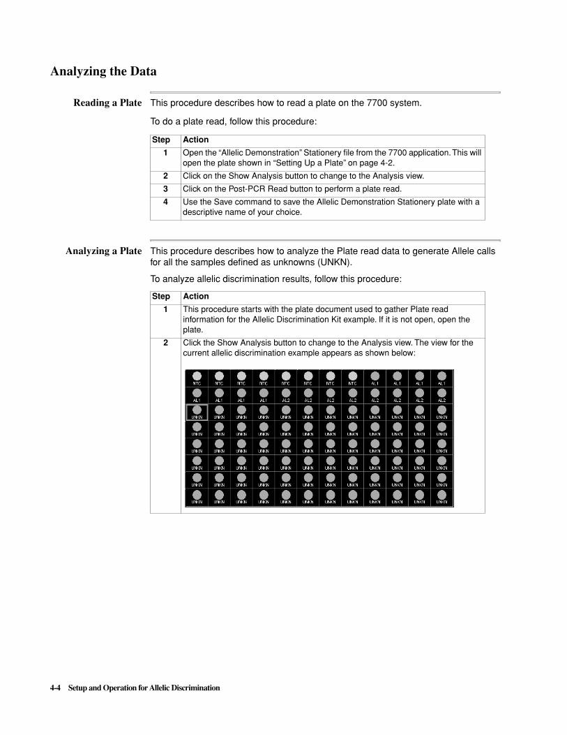
4-4 Setup and Operation for Allelic Discrimination
Analyzing the Data
Reading a Plate This procedure describes how to read a plate on the 7700 system.
To do a plate read, follow this procedure:
Analyzing a Plate This procedure describes how to analyze the Plate read data to generate Allele calls for all the samples defined as unknowns (UNKN).
Step Action
1 Open the “Allelic Demonstration” Stationery file from the 7700 application. This will open the plate shown in “Setting Up a Plate” on page 4-2.
2 Click on the Show Analysis button to change to the Analysis view.
3 Click on the Post-PCR Read button to perform a plate read.
4 Use the Save command to save the Allelic Demonstration Stationery plate with a descriptive name of your choice.
To analyze allelic discrimination results, follow this procedure:
Step Action
1 This procedure starts with the plate document used to gather Plate read information for the Allelic Discrimination Kit example. If it is not open, open the plate.
2 Click the Show Analysis button to change to the Analysis view. The view for the current allelic discrimination example appears as shown below:

Setup and Operation for Allelic Discrimination 4-5
3 Click Analyze (Analyze menu). This will initiate analysis and the view shown above will update to appear like this:
Note Analyzed data has the “hole” in the center.
4 Choose View Allelic Discrimination (Analysis menu) to produce the Allelic Discrimination Map for the run:
To analyze allelic discrimination results, follow this procedure: (continued)
Step Action
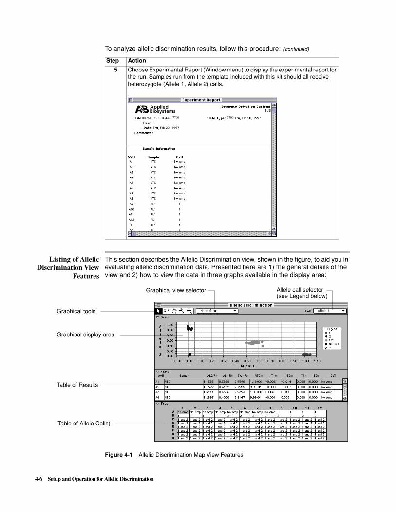
4-6 Setup and Operation for Allelic Discrimination
Listing of AllelicDiscrimination View
Features
This section describes the Allelic Discrimination view, shown in the figure, to aid you in evaluating allelic discrimination data. Presented here are 1) the general details of the view and 2) how to view the data in three graphs available in the display area:
Figure 4-1 Allelic Discrimination Map View Features
5 Choose Experimental Report (Window menu) to display the experimental report for the run. Samples run from the template included with this kit should all receive heterozygote (Allele 1, Allele 2) calls.
To analyze allelic discrimination results, follow this procedure: (continued)
Step Action
77007700
Graphical display area
Graphical view selector
Table of Results
Table of Allele Calls)
Allele call selector
Graphical tools
(see Legend below)
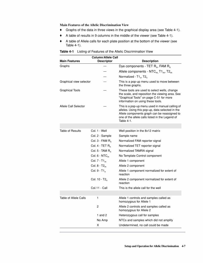
Setup and Operation for Allelic Discrimination 4-7
Main Features of the Allelic Discrimination View
� Graphs of the data in three views in the graphical display area (see Table 4-1).
� A table of results in 9 columns in the middle of the viewer (see Table 4-1).
� A table of Allele calls for each plate position at the bottom of the viewer (see Table 4-1).
Table 4-1 Listing of Features of the Allelic Discrimination View
Main FeaturesColumn/Allele Call
Descriptor Description
Graphs — Dye components - TET Rn, FAM Rn
— Allele components - NTCm, T1m, T2m
— Normalized - T1n, T2n
Graphical view selector — This is a pop-up menu used to move between the three graphs.
Graphical Tools — These tools are used to select wells, change the scale, and reposition the viewing area. See "Graphical Tools" on page C-51 for more information on using these tools.
Allele Call Selector — This is a pop-up menu used in manual calling of alleles. Using this pop-up, data selected in the Allele components graph can be reassigned to one of the allele calls listed in the Legend of Table 4-1.
Table of Results Col. 1 - Well Well position in the 8x12 matrix
Col. 2 - Sample Sample name
Col. 3 - FAM Rn Normalized FAM reporter signal
Col. 4 - TET Rn Normalized TET reporter signal
Col. 5 - TAM Rn Normalized TAMRA signal
Col. 6 - NTCm No Template Control component
Col. 7 - T1m Allele 1 component
Col. 8 - T2m Allele 2 component
Col. 9 - T1n Allele 1 component normalized for extent of reaction
Col. 10 - T2n Allele 2 component normalized for extent of reaction
Col.11 - Call This is the allele call for the well
Table of Allele Calls 1 Allele 1 controls and samples called as homozygous for Allele 1
2 Allele 2 controls and samples called as homozygous for Allele 2
1 and 2 Heterozygous call for samples
No Amp NTCs and samples which did not amplify
X Undetermined, no call could be made

4-8 Setup and Operation for Allelic Discrimination
Mathematical Transformations
Overview The 7700 system collects spectral data that ranges from 500nm to 660nm. We refer to this data as Raw Data. This data can be displayed graphically in the raw data view.
When running an Allelic Discrimination Analysis, the SDS software will run several mathematical transformations on the raw data. These transformations are used to generate a more direct measure of how the spectra changes relate to the control reactions (NTCs, Allele 1 and Allele 2 controls).
List of MathematicalTransformations
Transforming Raw Data into Dye Components
The first transformation made to the Raw Data is the same multicomponenting algorithm that is used for all SDS analysis.
This transformation takes the Raw data which is expressed in terms of Fluorescent Signal vs. Wavelength and, using the calibrated pure dye shapes as known, re-expresses the unknown sample in terms of the pure dye components.
In the allelic discrimination example we transform the raw data into the FAM, TET, TAMRA (TAM), and ROX components. The data is then all normalized by the ROX component and shown as FAM Rn, TET Rn, and TAM Rn in the allelic discrimination table as well as graphically (choose the Dye Component Graph within the allelic discrimination viewer).
Transforming Dye Component Data into Allele Components
The Second transformation allows us to correlate the spectra of the unknown samples into how much the spectra looks like our controls (NTCs, Allele 1 and Allele 2 controls). By measuring these controls we can determine what the spectra shape for each of these controls looks like, and by doing the first transformation we can even say what the dye components look like for each of the three control types.
By using the controls as inputs to our multicomponenting analysis, we can now transform the unknown sample data from how much the spectral shape looks like the dyes into how much the spectra looks like the controls.
These quantitative measures of the spectral shape are shown as NTCm, T1m, and T2m in the table and graphically (choose the Allele Components Graph within the allelic discrimination viewer).
Normalizing for the Extent of the Reaction
Our final mathematical transformation allows us to take an unknown sample and, based on the quantitative measure of how much the spectra looks like a No Template Control Reaction, we can scale the Allele 1 and Allele 2 components to create a measure of how much the reaction would look like Allele 1 and Allele 2 if all the reactions had the same amount of amplification occur.
These normalized components are shown as T1n and T2n in the table and graphically (choose the Normalized graph within the Allelic Discrimination viewer). The allele call (Homozygous 1, Homozygous 2 or Heterozygous) is determined from these normalized components.
Autocalling
Both the vertical and horizontal thresholds are calculated from the T-distribution using a 99.7% confidence level. The horizontal variation in the Allele 2 controls determines the vertical threshold and the vertical variation in the Allele 1 controls determines the horizontal threshold. The calls are made according to the following four zones:
� Allele1 call is made for data less than the horizontal threshold and greater than the vertical threshold.

Setup and Operation for Allelic Discrimination 4-9
� Allele 2 call is made for data greater than the horizontal threshold and less than the vertical threshold.
� Heterozygous 1/2 is made for data greater than both thresholds.
� No call is made for data less than both thresholds.
Making Manual Calls
Background You may choose to make manual calls for those wells that are labeled undetermined by the autocalling routine. You may also make manual calls for those data sets which have poor controls or an insufficient number of controls and the application will not autocall the data. By using the selector buttons in the Allele call selector you can manually select a group of data (or individual wells) and designate the allele call.
For data sets for which no autocalling is done, all the manual calls need to be made from the Dye Components View. There will be no data available in the other two views. For example, if the following event log was presented after analysis, you would know that autocalling had failed:
Note Whenever less than three controls are correctly identified, the system will present a log like that shown above. For information on how to use the tools in the Allelic Discrimination view as described in the following procedure, see “Allelic Discrimination” on page C-50.
continued on next page

4-10 Setup and Operation for Allelic Discrimination
Procedure This procedure is used to make manual calls whenever less than three controls are correctly identified.
To make manual calls when no autocalling was done:
Step Action
1 After you have analyzed your data (using the Analyze command from the Analysis menu), choose the Allelic Discrimination command (Analysis menu). You will be presented with an Allelic Discrimination view with no data shown.
2 Use the Graphical view selector to choose the Dye Components view (no data will be shown in the other two views).
3 Click the Plus Zoom button and then click the graphic view several times to zoom in and separate the data into distinct clumps.
If you click too many times, moving some data out of the view, click the Minus Zoom control and then click the graphical view again. You can also use the Position button to reposition displayed data while preserving the selected magnification.
4 Identify the data by clicking on a data point with the Individual data point selector or by selecting a data clump with the Group selector. The corresponding wells in the plate will be indicated below.
Note To select a data clump using the Group selector, position the selector near the clump, depress the mouse button, and draw a circle around the data.
5 After identifying data, make manual calls by selecting a data point or clump and then choose the proper call from the Allele call selector. The call you choose will be reflected for selected data in the plate matrix below the graphical view. (An alternative way to make calls for selected data is to use the Allele Calls command from the Analysis menu).
6 You will know you have correctly made calls when the assignments for Allele 1 and Allele 2 correspond to how you loaded the plate.
Your plate will look like Figure 4-2 after manual calling has been performed.

Setup and Operation for Allelic Discrimination 4-11
Figure 4-2 A Manually Called Allelic Discrimination Plate
Note The data represented as “?” (question marks) in the table and by X in the graphical view represents the failed control wells which necessitated the manual calling.
If any manual calls are made to your data, a note indicating that manual calls were made will be placed in your Experimental Report.
Allele 1 data
Allele 2 data
Allele 1/2 data


SR Plates, Plus/Minus Scoring, and IPCs 5-1
SR Plates, Plus/Minus Scoring, and IPCs 5
Introduction
General The Single Reporter (SR) Plate type is designed to report the presence or absence of a specific nucleic acid sequence in a test sample (Plus/Minus or +/- scoring). By using probes labeled with different reporters, a positive control for the PCR chemistry may be included in any amplification reaction. This Internal Positive Control (IPC) ensures that a failed PCR is not mistaken for a negative test result.
In This Chapter This chapter contains the following topics:
Topic See Page
Single Reporter Plates and Plus/Minus Scoring 5-2
Sample Type Setup 5-2
Statistics Settings 5-2
Analyzing Data 5-3
Reviewing Data 5-4
Experiment Report 5-5
Setting Up a Single Reporter Plate with an IPC Dye Layer 5-7
Sample Type Setup 5-7
Statistics Settings/Analyzing Data 5-7
Reviewing Data 5-8
Experiment Report 5-9
5
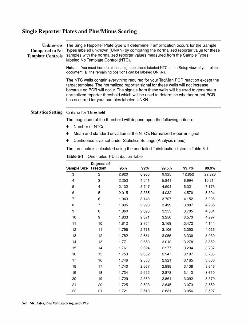
5-2 SR Plates, Plus/Minus Scoring, and IPCs
Single Reporter Plates and Plus/Minus Scoring
UnknownsCompared to No
Template Controls
The Single Reporter Plate type will determine if amplification occurs for the Sample Types labeled unknown (UNKN) by comparing the normalized reporter value for these samples with the normalized reporter values measured from the Sample Types labeled No Template Control (NTC).
Note You must include at least eight positions labeled NTC in the Setup view of your plate document (all the remaining positions can be labeled UNKN).
The NTC wells contain everything required for your TaqMan PCR reaction except the target template. The normalized reporter signal for these wells will not increase because no PCR will occur. The signals from these wells will be used to generate a normalized reporter threshold which will be used to determine whether or not PCR has occurred for your samples labeled UNKN.\
Statistics Setting Criteria for Threshold
The magnitude of the threshold will depend upon the following criteria:
� Number of NTCs
� Mean and standard deviation of the NTC’s Normalized reporter signal
� Confidence level set under Statistics Settings (Analysis menu)
The threshold is calculated using the one-tailed T-distribution listed in Table 5-1.
Table 5-1 One-Tailed T-Distribution Table
Sample SizeDegrees of Freedom 95% 99% 99.5% 99.7% 99.9%
3 2 2.920 6.965 9.925 12.852 22.328
4 3 2.353 4.541 5.841 6.994 10.214
5 4 2.132 3.747 4.604 5.321 7.173
6 5 2.015 3.365 4.032 4.570 5.894
7 6 1.943 3.143 3.707 4.152 5.208
8 7 1.895 2.998 3.499 3.887 4.785
9 8 1.860 2.896 3.355 3.705 4.501
10 9 1.833 2.821 3.250 3.573 4.297
11 10 1.812 2.764 3.169 3.472 4.144
12 11 1.796 2.718 3.106 3.393 4.025
13 12 1.782 2.681 3.055 3.330 3.930
14 13 1.771 2.650 3.012 3.278 3.852
15 14 1.761 2.624 2.977 3.234 3.787
16 15 1.753 2.602 2.947 3.197 3.733
17 16 1.746 2.583 2.921 3.165 3.686
18 17 1.740 2.567 2.898 3.138 3.646
19 18 1.734 2.552 2.878 3.113 3.610
20 19 1.729 2.539 2.861 3.092 3.579
21 20 1.725 2.528 2.845 3.073 3.552
22 21 1.721 2.518 2.831 3.056 3.527

SR Plates, Plus/Minus Scoring, and IPCs 5-3
Procedure
To change the confidence level from the default value of 99.7%:
Initiating Analysis When you have collected your data and set your desired confidence level, you are ready to initiate analysis.
� To analyze data, choose Analyze from the Analysis menu.
Note Information regarding the analysis is recorded automatically in the Event Log.
continued on next page
23 22 1.717 2.508 2.819 3.041 3.505
24 23 1.714 2.500 2.807 3.027 3.485
25 24 1.711 2.492 2.797 3.014 3.467
26 25 1.708 2.485 2.787 3.003 3.450
27 26 1.706 2.479 2.779 2.992 3.435
28 27 1.703 2.473 2.771 2.982 3.421
29 28 1.701 2.467 2.763 2.973 3.408
30 29 1.699 2.462 2.756 2.965 3.396
31 30 1.697 2.457 2.750 2.957 3.385
32 to 41 40 1.684 2.423 2.704 2.902 3.307
42 to 61 60 1.671 2.390 2.660 2.849 3.232
62 to 121 120 1.658 2.358 2.617 2.798 3.160
122 and above
Infinite 1.645 2.326 2.576 2.748 3.090
Step Action
1 Choose Statistics Settings (Analyze menu) to bring up the dialog box shown below.
2 Click the new confidence level value.
3 Click OK to close this dialog box.
The new confidence level will be used when you analyze the plate.
Table 5-1 One-Tailed T-Distribution Table (continued)
Sample SizeDegrees of Freedom 95% 99% 99.5% 99.7% 99.9%

5-4 SR Plates, Plus/Minus Scoring, and IPCs
Reviewing Data After PCR is complete and your data is collected and analyzed, the Sequence Detection application program provides both graphic views of the data and an Experiment Report with the normalized reporter signal values, as well as a +/– PCR call for all your unknowns.
Raw Spectra Graph
Raw data is available for viewing before or after analysis and is viewed in the Raw Spectra view.
Figure 5-1 Raw Spectra View
The Raw Spectra view displays the 32 discrete wavelength intensities measured for each selected sample well. You can view the data from a single well or from multiple wells. For more information on viewing options, see Raw Spectra on page C-55.
Analysis Plate View (Target Dye Layer)
After analyzing the data, the intensity of each circle corresponds to the Rn value. You can modify the intensity controls using the Rn range controls (max and min).
To change the display from Sample Type to Rn (normalized reporter signal) for each well, choose Rn under Display in the Analysis menu.
continued on next page
Table 5-2 Where to Find Data in the Sequence Detection Application Program
Available Data Graphic View Analysis Plate View Experiment Report
Raw data Raw Spectra — —
Replicate Calculations
— — Mean & Deviation.
+/– results — — +/– listed for all wells
DRn or Rn — Values and intensities Values

SR Plates, Plus/Minus Scoring, and IPCs 5-5
ExperimentReport
General
The Experiment Report displays relevant setup information and the calculated values listed below for all wells of the plate document.
� PCR call: results indicated by a “+” (PCR detected) or “–” (no PCR detected)
� Rn: the normalized reporter
� Standard deviation of each replicate group
� Mean value of each replicate group
The Experiment Report is only available after analyzing (choosing Analyze from the Analysis menu). When you close the plate document, the analyzed data is not saved, so you must reanalyze the data each time you open the plate document to regenerate the Experiment Report.
Viewing, Printing, and Exporting the Experiment Report
You can view, print, and export the Experiment Report.
To view the Experiment Report, choose Experiment Report from the Window menu.
As shown in Figure 5-2, the Experiment Report window opens and becomes the active window on the computer screen. You can scroll through the contents of the window to review the report, but you cannot edit the text.
Figure 5-2 Single Reporter Experiment Report
Note The Experiment Report above did not include an IPC dye layer. See Figure 5-6 for the information which is added when an IPC layer is present.

5-6 SR Plates, Plus/Minus Scoring, and IPCs
To print the Experiment Report, do the following :
To export the Experiment Report, do the following:
Step Action
1 Click the Experiment Report window to make it active.
2 Choose Page Setup from the File menu.
3 Click the Landscape orientation icon and reduce the size of the page to 95%.
4 Click OK to close the Page Setup dialog box.
5 Choose Print from in the File menu and click Print.
Step Action
1 Choose Experiment Report from the Export options under File menu.
2 In the File dialog box, give the report a descriptive name and click OK.

SR Plates, Plus/Minus Scoring, and IPCs 5-7
Setting Up a Single Reporter Plate with an IPC Dye Layer
Sample Type Setup A Single Reporter IPC experiment uses two TaqMan probes and therefore requires sample setup on two dye layers. The Sample Type setup for the target probe dye layer is identical to that of a standard Single Reporter plate (refer to the previous setup for the target layer). The IPC probe layer requires the IPC+ and IPC– sample types.
You must include at least eight positions labeled IPC– on the IPC dye layer (all the remaining positions on this layer can be labeled IPC+). The application program will determine if amplification of the IPC occurs for the Sample Types labeled IPC+ by comparing the normalized reporter value for these samples with the normalized reporter values measured from the Sample Types labeled IPC–.
The IPC– wells contain everything required for your TaqMan PCR reaction except the IPC template. The normalized reporter signal for the IPC dye layer for these wells will not increase because no amplification of the IPC will occur. The signals from these wells will be used to generate a normalized reporter threshold which will be used to determine whether or not PCR has occurred for your samples labeled IPC+.
Figure 5-3 Typical IPC Layer setup
Note You may either add the IPC– and IPC+ Sample Types to a standard Single Reporter Plate document (see Guidelines for IPC on page C-39) or you may open the Single Reporter IPC Stationery document. For the analysis to work properly, you must correspond exactly to our acronym naming conventions.
\
StatisticsSettings/Analyzing
Data
Criteria for Thresholds
The magnitude of the thresholds will depend upon the following criteria:
� Number of NTCs and number of IPC– controls
� Means and standard deviations of the corresponding Normalized reporter signals for the NTCs and IPC– controls
� Confidence level set under Statistics Settings (Analysis menu)
The thresholds are calculated using the same T-distribution table (see Table 5-1 on page 5-2).
To change the confidence level from the default value of 99%, choose Statistics Settings (Analyze menu). See page 5-2 for information on setting Statistics.

5-8 SR Plates, Plus/Minus Scoring, and IPCs
Initiating Analysis
When you have collected your data and set your desired confidence level, you are ready to initiate analysis. To analyze data, choose Analyze from the Analysis menu, or use the keyboard shortcut c L.
Note Information regarding the analysis will automatically be presented in the Event Log.
Reviewing Data After PCR is complete and your data is collected and analyzed, the Sequence Detection application program provides graphic views of the data and an Experiment Report with the normalized reporter signal values as well as a +/– /No Amp PCR call for all your unknowns. A false negative, indicated by a “No Amp” or “?” call, is a reaction where PCR did not occur on either the target or the IPC layers. A true negative, indicated by “-”, is a reaction where PCR did not occur on the target but did occur on the IPC layer.
Raw Spectra Graph
See the Single Reporter description on page 5-8.
Analysis Plate View
Before starting a plate read, all active wells are displayed as solid colored circles. After a plate read, the display of all the active wells changes to a solid color whose intensity corresponds to the fluorescence data collected.
Target Dye Layer
After analyzing the data, the intensity of each circle corresponds to the Rn value. You can modify the intensity controls using the Rn range controls (max and min).
To change the display from Sample Type to Rn (normalized reporter signal) for each well, choose Rn under Display in the Analysis menu.
Figure 5-4 Rn in the Analysis View
Table 5-3 Where to Find Data in the Sequence Detection Application Program
Available Data Graphic View Analysis Plate View Experiment Report
Raw data Raw Spectra — —
Replicate calculations
— — Mean & std. dev.
+/– results — +/–/? calls shown onIPC layer
+/–/? or No Amp listed for all wells
DRn or Rn — Values and intensities shown on the target layer
Values

SR Plates, Plus/Minus Scoring, and IPCs 5-9
IPC Dye Layer
After analyzing the data, a “+”, “–”, or “?” symbol is placed in the solid dot shown on the IPC dye layer.
Figure 5-5 IPC dye layer after analysis
� + indicates that PCR occurred.
� – indicates a true negative (no PCR occurred on target layer but PCR did occur for IPC).
� ? indicates a false negative (no PCR occurred for either the target or the IPC).
Experiment Report The Experiment Report displays relevant setup information and the following calculated values for all wells of the plate document.
The Experiment Report for “+/-” scoring includes a “No Amp” call, distinguishing a false negative from a true negative. A true negative will be marked with a “–” and a false negative will be marked No Amp in the PCR column.
Figure 5-6 Experiment Report for Single Reporter with IPC
Note The above Single Reporter report was produced by a plate read and did not perform PCR. If PCR had been performed using an IPC dye layer, the report would also contain the Thermal Cycler Condition information as well as other information shown in Figure 5-2.
The Experiment Report is only available after analyzing. You can view, print, and export this report (see page 5-5).


Troubleshooting and Maintenance 6-1
Troubleshooting and Maintenance 6
Introduction
General This section provides two tables. Use the first table when either your Macintosh computer or the Sequence Detection application program will not run. Use the second table when the application program launches but will not run properly.
In This Chapter This chapter covers the following topics:
Topic See Page
Macintosh and General Troubleshooting 6-2
Troubleshooting Table 6-2
7700 Sequence Detection System Troubleshooting 6-4
Troubleshooting Table 6-4
System Requirements and Known Software Bugs 6-6
Software and Firmware Revisions 6-6
Power Macintosh Specifications 6-6
System Noise 6-6
9600 Specifications 6-6
Reporting Software Bugs 6-7
Quick System Tests 6-8
Fluorescence Tests (Signal Throughput) 6-8
Blackboard Tests (Background Signal) 6-9
9600 Tests 6-10
6
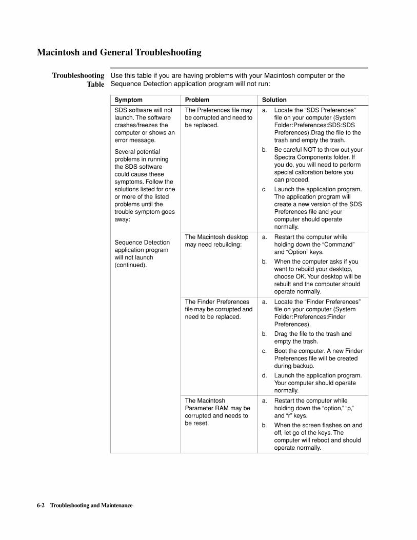
6-2 Troubleshooting and Maintenance
Macintosh and General Troubleshooting
TroubleshootingTable
Use this table if you are having problems with your Macintosh computer or the Sequence Detection application program will not run:
Symptom Problem Solution
SDS software will not launch. The software crashes/freezes the computer or shows an error message.
Several potential problems in running the SDS software could cause these symptoms. Follow the solutions listed for one or more of the listed problems until the trouble symptom goes away:
Sequence Detection application program will not launch (continued).
The Preferences file may be corrupted and need to be replaced.
a. Locate the “SDS Preferences” file on your computer (System Folder:Preferences:SDS:SDS Preferences).Drag the file to the trash and empty the trash.
b. Be careful NOT to throw out your Spectra Components folder. If you do, you will need to perform special calibration before you can proceed.
c. Launch the application program. The application program will create a new version of the SDS Preferences file and your computer should operate normally.
The Macintosh desktop may need rebuilding:
a. Restart the computer while holding down the “Command” and “Option” keys.
b. When the computer asks if you want to rebuild your desktop, choose OK. Your desktop will be rebuilt and the computer should operate normally.
The Finder Preferences file may be corrupted and need to be replaced.
a. Locate the “Finder Preferences” file on your computer (System Folder:Preferences:Finder Preferences).
b. Drag the file to the trash and empty the trash.
c. Boot the computer. A new Finder Preferences file will be created during backup.
d. Launch the application program. Your computer should operate normally.
The Macintosh Parameter RAM may be corrupted and needs to be reset.
a. Restart the computer while holding down the “option,” “p,” and “r” keys.
b. When the screen flashes on and off, let go of the keys. The computer will reboot and should operate normally.
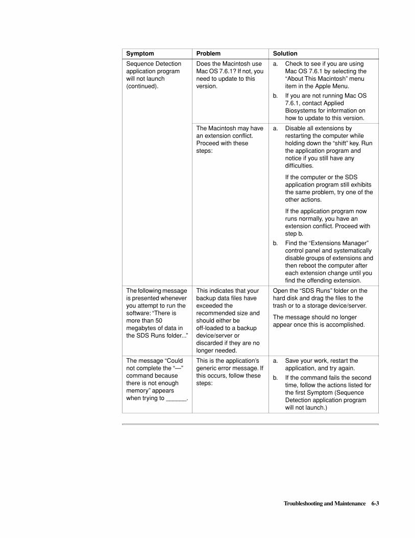
Troubleshooting and Maintenance 6-3
Sequence Detection application program will not launch (continued).
Does the Macintosh use Mac OS 7.6.1? If not, you need to update to this version.
a. Check to see if you are using Mac OS 7.6.1 by selecting the “About This Macintosh” menu item in the Apple Menu.
b. If you are not running Mac OS 7.6.1, contact Applied Biosystems for information on how to update to this version.
The Macintosh may have an extension conflict. Proceed with these steps:
a. Disable all extensions by restarting the computer while holding down the “shift” key. Run the application program and notice if you still have any difficulties.
If the computer or the SDS application program still exhibits the same problem, try one of the other actions.
If the application program now runs normally, you have an extension conflict. Proceed with step b.
b. Find the “Extensions Manager” control panel and systematically disable groups of extensions and then reboot the computer after each extension change until you find the offending extension.
The following message is presented whenever you attempt to run the software: “There is more than 50 megabytes of data in the SDS Runs folder...”
This indicates that your backup data files have exceeded the recommended size and should either be off-loaded to a backup device/server or discarded if they are no longer needed.
Open the “SDS Runs” folder on the hard disk and drag the files to the trash or to a storage device/server.
The message should no longer appear once this is accomplished.
The message “Could not complete the “—” command because there is not enough memory” appears when trying to ______.
This is the application’s generic error message. If this occurs, follow these steps:
a. Save your work, restart the application, and try again.
b. If the command fails the second time, follow the actions listed for the first Symptom (Sequence Detection application program will not launch.)
Symptom Problem Solution

6-4 Troubleshooting and Maintenance
7700 Sequence Detection System Troubleshooting
TroubleshootingTable
Use this table when you have been running the ABI PRISM® 7700 Sequence Detection System and the listed symptom occurs:
Symptom Problem Solution
Application program will not connect to the 7700 instrument.
The cable connection between the computer and instrument is faulty or the cable is disconnected:
Check the cable connection.
The open plate document may not be an “online” document.
Make sure the document is an “online” document by going to “Preferences” (Edit Menu) and activating the “Online Document” checkbox.
The computer seems to “freeze” periodically while running the Sequence Detection application program.
Updating to Mac OS 7.6.1 helps reduce freezes or system lockups on a Macintosh running earlier operating systems.
a. Check to see if you are using Mac OS 7.6.1 by selecting the “About This Macintosh” menu item in the Apple Menu.
b. If you are not running Mac OS 7.6.1, contact Applied Biosystems for information on how to update to this version.
The Experiment Report is empty.
Only raw data is saved in the plate document, so you must re-analyze the plate to see report data.
Re-analyze data each time you open a plate document to generate the Experiment Report.
When launching the program, the following dialog box appears:
The necessary Pure Dye files for FAM, TAMRA, and ROX are not available.
You need to measure and extract Pure Dye files for FAM, TAMRA, and ROX. See calibration procedure on page 3-10.
Specific wells consistently read incorrectly.
The Sample Block is dirty. Using a cotton swab, wipe the wells with a 10% bleach solution. Using a second swab, dry by swabbing with 95% ethanol.
Raw spectra signal is flat at an intensity of 10,000.
The sample has too high of a concentration.
Dilute your sample.

Troubleshooting and Maintenance 6-5
No Read button is visible in the Analysis View although a non-functioning Run button is present.
You are attempting to use a plate type set up for a Real Time run.
You need to define the correct instrument type as follows:
a. Close the current plate.
b. Open a new plate of the desired type.
Symptom Problem Solution

6-6 Troubleshooting and Maintenance
System Requirements and Known Software Bugs
Software andFirmware Revisions
SDS Software Revision 1.0 or 1.6 (“b”, “d”, or “fc” versions are not supported).
Firmware M13 (EPROM) or M14 (EPROM or downloaded to battery backed-up RAM).
Note Unreleased or developmental versions of the SDS Application are not supported by Applied Biosystems personnel (Technical Support and Field Applications Specialists): use only released software versions when servicing the 7700.
Power MacintoshSpecifications
RAM
At least 24 MB of RAM (DIMMs).
IMPORTANT DIMMs (Dual in-line memory modules) must be matched for speed (in MHz).
IMPORTANT Do not use Virtual Memory to make up for missing DIMMs. Virtual Memory must not be used during data collection.
Macintosh Operating System
Version 7.6.1
IMPORTANT Macintosh O.S. 7.5.2 can cause serious operational problems.
System Noise Maximum signal of 1200 on any optical fiber when running the LabView-based 7700 Service Diagnostics with a clean Blackboard or a new 96-well tray of water.
9600 Specifications EPROMs
The 9600 portion of the 7700 instrument must use special EPROMs: see “Service of the Thermal Cycler” in the Service Procedures section of this manual for more information.
Voltage and Frequency Configuration
The thermal cycler operates on 230Vac (supplied from the Vac Distribution Assembly) but it must be configured for the proper frequency (either 50 or 60 Hz). A 36-pin voltage select plug is inserted into J-13 on the AC-Control PCB in the 9600: the plug has 5 jumpers with each wire connecting 2 pins. The 230V/50 Hz plug has pins 2/5, 9/17, 28/34, 31/36, and 33/35 jumpered. The 230V/60 Hz plug has pins 2/5, 9/16, 28/34, 31/36, and 33/35 jumpered.
CAUTION Damage to the 9600 instrument electronics or firmware could occur if the wrong voltage configuration plug is inserted into J-13. Always check the wiring of the 9600 instrument voltage configuration plug before installing it.
Temperature Verification
The thermal cycler conforms to the 9600 Temperature Verification Specifications as described in the 9600 Service Manual. See that service manual for more information.
Note Thermal cycler service should be done only by ABD-trained, 7700 instrument trained, service personnel. 9600 service training does not cover all aspects of servicing the 7700 instrument’s thermal cycler.
continued on next page

Troubleshooting and Maintenance 6-7
Reporting SoftwareBugs
The following is a list of known software bugs that can be encountered when using SDS Version 1.6 Software. If other bugs are discovered, always try to reproduce the bug. Report any bugs to Applied Biosystems SDS Technical Support.
� After generating the Background Component, you must quit the SDS application before generating the Pure Dyes file or the background will not be recognized.
� If a dialog box appears at launch stating “Could not start application because a file has been left in use”’ or some other similar message, then trash the SDS Preferences (System Folder: Preferences: SDS) and re-launch the application.
� If the instrument Status is “Waiting...” do not attempt to stop the instrument until “Ramping” or “Holding” is seen in the Status display. If you stop the instrument during this time, the instrument will begin to “beep” and you will have to reset the instrument and computer to correct the problem.
� When editing the “Advanced Options” dialog box and click “OK” to exit, another dialog box stating “You must restart for changes to take effect” appears. This is only true if you change the checkboxes for “Analysis: Spectra Components”:
– If you change other options, those changes will take effect immediately.
� A “Firmware Version Conflict” will be noted if the instrument boots off the EPROM (Firmware versions M12 and M13) OR if the 7700’s battery is dead: keep the 7700 instrument turned ON to prevent the loss of firmware stored in the 7700’s RAM.
� The “Spooled Items” folder (System Folder: Preferences: SDS) is now used ONLY to store data that would otherwise be lost in the event of a powerfail.

6-8 Troubleshooting and Maintenance
Quick System Tests
Fluorescence Tests(Signal Throughput)
Fluorescent Tests (Red Fluorescent Source)
If a T-6222 test tray is not available, then quick results can also be obtained by scanning any fluorescent source for 1 minute at 25 degrees C: results will vary depending on the type of tray being scanned.
IMPORTANT Blue test trays or paper can be used to confirm signal throughput, but they should NOT be used to confirm laser alignment.
Note Signal heights of the fibers will vary depending on the well position, the specific 7700 instrument being used, and type of tray being used and the temperature of the test tray.
Figure 6-1 Fluorescent results using a red test tray (example)
continued on next page

Troubleshooting and Maintenance 6-9
Blackboard Tests(Background Signal)
The background signal of the system can be investigated in many different ways. When using a Blackboard or some other black test tray (also, scanning the CCD with either the shutters closed or the MUX at position #0), the results obtained will give you an indication of the background from the test tray, lenses, fibers, and the CCD.
Note Signal heights of the fibers will vary depending on the well position, the specific 7700 instrument being used, and the temperature of the test tray. Results obtained from using a blackboard do not take into account any interference from the sample block or real PCR samples.
Figure 6-2 Fluorescent results using a Blackboard (black test tray example - 1 minute, 25 °C)
Note Instrument System tests are done using the Functions Test dialog box. See “Functions Test” on page C-45 for more information.
continued on next page

6-10 Troubleshooting and Maintenance
9600 Tests The easiest way to check the thermal cycler is to look at a runs’s thermal cycler profile found whenever you view Raw Data or Multicomponent Data.
Figure 6-3 Thermal cycler profile (example)
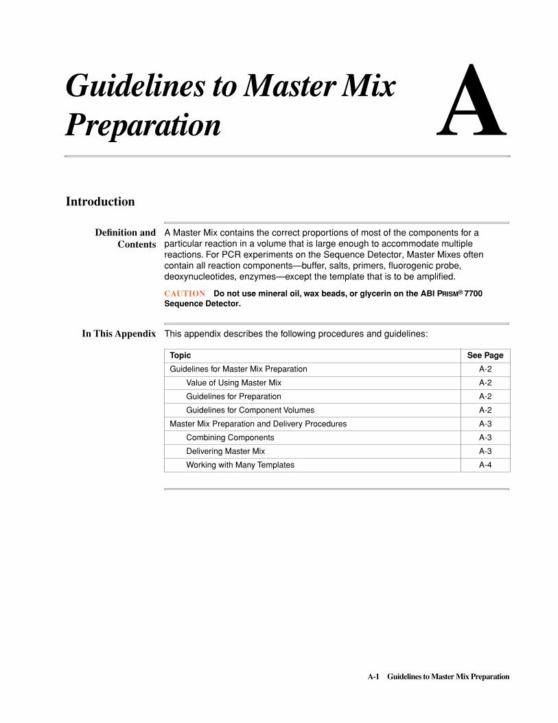
A-1 Guidelines to Master Mix Preparation
Guidelines to Master Mix Preparation A
Introduction
Definition andContents
A Master Mix contains the correct proportions of most of the components for a particular reaction in a volume that is large enough to accommodate multiple reactions. For PCR experiments on the Sequence Detector, Master Mixes often contain all reaction components—buffer, salts, primers, fluorogenic probe, deoxynucleotides, enzymes—except the template that is to be amplified.
CAUTION Do not use mineral oil, wax beads, or glycerin on the ABI PRISM® 7700 Sequence Detector.
In This Appendix This appendix describes the following procedures and guidelines:
Topic See Page
Guidelines for Master Mix Preparation A-2
Value of Using Master Mix A-2
Guidelines for Preparation A-2
Guidelines for Component Volumes A-2
Master Mix Preparation and Delivery Procedures A-3
Combining Components A-3
Delivering Master Mix A-3
Working with Many Templates A-4
A
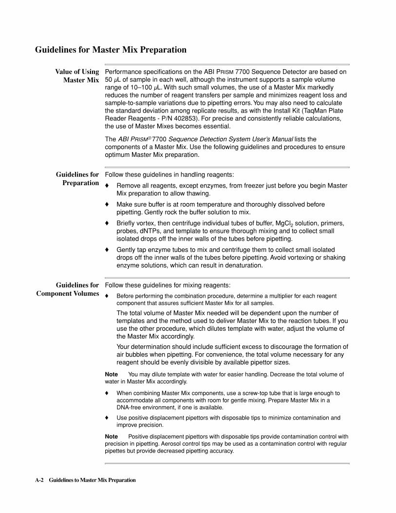
A-2 Guidelines to Master Mix Preparation
Guidelines for Master Mix Preparation
Value of UsingMaster Mix
Performance specifications on the ABI PRISM 7700 Sequence Detector are based on 50 µL of sample in each well, although the instrument supports a sample volume range of 10–100 µL. With such small volumes, the use of a Master Mix markedly reduces the number of reagent transfers per sample and minimizes reagent loss and sample-to-sample variations due to pipetting errors. You may also need to calculate the standard deviation among replicate results, as with the Install Kit (TaqMan Plate Reader Reagents - P/N 402853). For precise and consistently reliable calculations, the use of Master Mixes becomes essential.
The ABI PRISM® 7700 Sequence Detection System User’s Manual lists the components of a Master Mix. Use the following guidelines and procedures to ensure optimum Master Mix preparation.
Guidelines forPreparation
Follow these guidelines in handling reagents:
� Remove all reagents, except enzymes, from freezer just before you begin Master Mix preparation to allow thawing.
� Make sure buffer is at room temperature and thoroughly dissolved before pipetting. Gently rock the buffer solution to mix.
� Briefly vortex, then centrifuge individual tubes of buffer, MgCl2 solution, primers, probes, dNTPs, and template to ensure thorough mixing and to collect small isolated drops off the inner walls of the tubes before pipetting.
� Gently tap enzyme tubes to mix and centrifuge them to collect small isolated drops off the inner walls of the tubes before pipetting. Avoid vortexing or shaking enzyme solutions, which can result in denaturation.
Guidelines forComponent Volumes
Follow these guidelines for mixing reagents:
� Before performing the combination procedure, determine a multiplier for each reagent component that assures sufficient Master Mix for all samples.
The total volume of Master Mix needed will be dependent upon the number of templates and the method used to deliver Master Mix to the reaction tubes. If you use the other procedure, which dilutes template with water, adjust the volume of the Master Mix accordingly.
Your determination should include sufficient excess to discourage the formation of air bubbles when pipetting. For convenience, the total volume necessary for any reagent should be evenly divisible by available pipettor sizes.
Note You may dilute template with water for easier handling. Decrease the total volume of water in Master Mix accordingly.
� When combining Master Mix components, use a screw-top tube that is large enough to accommodate all components with room for gentle mixing. Prepare Master Mix in a DNA-free environment, if one is available.
� Use positive displacement pipettors with disposable tips to minimize contamination and improve precision.
Note Positive displacement pipettors with disposable tips provide contamination control with precision in pipetting. Aerosol control tips may be used as a contamination control with regular pipettes but provide decreased pipetting accuracy.

Guidelines to Master Mix Preparation A-3
Master Mix Preparation and Delivery Procedures
CombiningComponents
Use the following procedure to combine components:
Delivering MasterMix
General
Researchers have devised many methods for delivering Master Mix among 96 sample tubes. The criteria for determining the most appropriate method are subjective and highly personal. The following two methods have been used successfully in our research labs.
Working with Few Templates
This first method works well when fewer than ten templates are being distributed across a 96-well plate, as with the Install Kit. In this method, divide Master Mix among as many tubes as there are templates and controls. The following procedure uses the Install Kit as an example, though it can be applied to other experiments.;
Step Action
1 Deliver components to the Master Mix tube. Always add enzymes last.
2 Replace the screw-on cap on the Master Mix tube after each component is added to minimize contamination.
3 Deliver each reagent directly into the solution. Avoid delivering down the inner sides of the Master Mix tube.
4 When all components but the enzymes have been added to the Master Mix, replace the screw-on cap and vortex the Master Mix briefly at a low speed.
5 Slowly deliver enzymes, which tend to be viscous, directly into the Master Mix with the disposable tip in the solution. When you have delivered all enzyme, keep the tip in the solution and slowly pump the pipettor twice to rinse out the tip.
6 When all components except the template have been added, screw the cap tightly on the Master Mix tube and gently rock the tube to mix.
To deliver the Master Mix to fewer than ten templates, follow this procedure:
Step Action
1 Label one tube for each template. With the Install Kit, there are five standards, one No Template control, and two Unknowns, so label eight tubes, one for each template plus the No Template control.
2 Divide the Master Mix among the eight tubes, according to the directions in the Install Kit. The volume in each tube should allow 45 µL for each sample replicate plus sufficient extra volume to avoid bubble formation while pipetting.
With the Install Kit, you must add 4 x 45 µL plus extra dead volume for each DNA Template and for the No Template control. For each of the unknowns, add 36 x 45 µL, plus extra dead volume.
3 Add each template to the appropriately labeled tube. The volume of template added should be sufficient to maintain the 5:45 (template-to-Master Mix) volume ratio.
4 Work with template solutions of low concentrations before working with more concentrated template solutions. Cap each tube as soon as you finish adding template to deter contamination from more concentrated solutions.

A-4 Guidelines to Master Mix Preparation
Working with ManyTemplates
This second method has been suggested for experiments that have more than ten templates on a 96-well plate. In this method, you first deliver the appropriate amount of diluted template to each sample tube. Then you deliver Master Mix solution on top of the diluted template. Because the Master Mix solution has a higher density than the template solution, the two solutions mix somewhat as the Master Mix is added.
Note You may dilute template with water for easier handling. Decrease the total volume of water in Master Mix accordingly.
When using this method, calculate in advance of preparing the Master Mix how much water you will use to dilute all the templates. Subtract this volume of water from the total amount of water needed to prepare the Master Mix.
To deliver Master Mix and diluted templates for more than ten templates, follow this procedure:
5 Slowly deliver template, which may be viscous, directly into the Master Mix with the disposable tip in the solution. When you have delivered all template, keep the tip in the solution and slowly pump the pipettor twice to rinse out the tip.
6 Screw the caps tightly on each tube of template solution and gently rock the tubes to mix.
7 Set up all reaction tubes in the tube holder. Make sure sample tube A1 is in the upper-left corner of the sample tube holder.
8 Use a repeater pipette with a disposable displacement tip to deliver 50 µL of each template solution to a reaction tube.
To deliver the Master Mix to fewer than ten templates, follow this procedure: (continued)
Step Action
Step Action
1 Prepare the Master Mix, adjusting the total volume of water for the amount of water needed to dilute all templates.
2 Dilute each template.
3 Make sure sample tube A1 is in the upper-left corner of the sample tube holder.
4 Deliver diluted templates to appropriate sample tubes.
5 Use a positive displacement pipettor with disposable tips to deliver Master Mix to sample tubes.

Purification of DNA B-1
Purification of DNA B
Introduction
General This appendix covers the use of the GeneBinder and QIAmp procedures to purify DNA. For RNA, an extraction method that provides sufficiently clean RNA for PCR should be adequate for the 5´ nuclease assay.
In This Appendix The following topics are included in this appendix:
Topic See Page
Background and Requirements B-2
Recommendation of Two Procedures B-2
GenePure BaseBinder B-2
QIAmp Protocol B-2
Purification B-2
Required Equipment B-3
Required Reagents B-3
Preparation of Reagent Solutions and Samples B-5
Instructions for Preparing Reagents B-5
Preparing Samples for Purification B-6
Preparing Cultured Cells B-7
Preparing Tissue Samples B-7
Purifying DNA: The GenePure BaseBinder Procedure B-8
Lysing and Digesting Cells B-8
Isolating Genomic DNA with BaseBinder B-8
Purifying DNA: The QIAmp Procedure B-11
General B-11
Procedures B-11
Determining DNA Quality B-12
UV Spectroscopy B-12
B
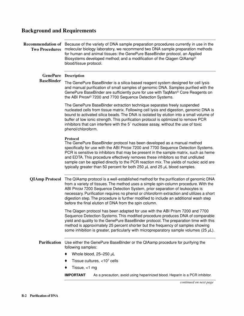
B-2 Purification of DNA
Background and Requirements
Recommendation ofTwo Procedures
Because of the variety of DNA sample preparation procedures currently in use in the molecular biology laboratory, we recommend two DNA sample preparation methods for human and animal tissues: the GenePure BaseBinder protocol, an Applied Biosystems developed method; and a modification of the Qiagen QIAamp® blood/tissue protocol.
GenePureBaseBinder
Description
The GenePure BaseBinder is a silica-based reagent system designed for cell lysis and manual purification of small samples of genomic DNA. Samples purified with the GenePure BaseBinder are sufficiently pure for use with TaqMan® Core Reagents on the ABI PRISM® 7200 and 7700 Sequence Detection Systems.
The GenePure BaseBinder extraction technique separates freely suspended nucleated cells from tissue matrix. Following cell lysis and digestion, genomic DNA is bound to activated silica beads. The DNA is isolated by elution into a small volume of buffer of low ionic strength. This purification protocol is optimized to remove PCR inhibitors that can interfere with the 5´ nuclease assay, without the use of toxic phenol/chloroform.
ProtocolThe GenePure BaseBinder protocol has been developed as a manual method specifically for use with the ABI PRISM 7200 and 7700 Sequence Detection Systems. PCR is sensitive to inhibitors that may be present in the sample matrix, such as heme and EDTA. This procedure effectively removes these inhibitors so that undiluted sample can be applied directly to the PCR reaction mix. The yields of nucleic acid are typically greater than 50 percent for both 250 µL and 25 µL blood samples.
QIAmp Protocol The QIAamp protocol is a well-established method for the purification of genomic DNA from a variety of tissues. The method uses a simple spin-column procedure. With the ABI PRISM 7200 Sequence Detection System, prior separation of leukocytes is necessary. Purification requires no phenol or chloroform extraction and utilizes a short digestion step. The procedure is further modified to include an additional wash step before the final elution of DNA from the spin column.
The Qiagen protocol has been adapted for use with the ABI Prism 7200 and 7700 Sequence Detection Systems. This modified procedure produces DNA of comparable yield and quality to the GenePure BaseBinder protocol. The preparation time with this method is approximately 25 percent shorter but the frequency of samples showing some inhibition is greater, particularly with micropreparatory sample volumes (25 µL).
Purification Use either the GenePure BaseBinder or the QIAamp procedure for purifying the following samples:
� Whole blood, 25–250 µL
� Tissue cultures, <107 cells
� Tissue, <1 mg
IMPORTANT As a precaution, avoid using heparinized blood. Heparin is a PCR inhibitor.
continued on next page

Purification of DNA B-3
Required Equipment The required equipment is listed in Table B-1:
Required Reagents The required reagents are listed in Table B-2:
Note Use analytical-reagent (AR) grade buffer salts and reagents, or their equivalents.
For chemicals required for this instrument but not manufactured or sold by Applied Biosystems, obtain the MSDSs from their manufacturers. For an MSDS for TaqMAN® PCR Core Reagents supplied with the instrument, see the ABI PRISM® 7700 Sequence Detection System Site Preparation and Safety Guide.
Table B-1 List of Required Equipment
Item Source
Microcentrifuge, large capacity, 1.5-mL tube Brinkman Model 5416 (P/N 22-62-200-5, with 24 place fixed angle rotator (P/N 22-63-220-5), or equivalent
Heater-shaker, (combination vortex and heating block) multi-sample, temperature range: ambient to 95 °C
Brinkman Model 5436
Tissue grinder, disposable Kimble/Kontes (P/N 95050-99) or equivalent
Pipettor, repeater, delivery volume: 25 µL–1000 µL Eppendorf Model 4780
Microcentrifuge tubes, sterile, 1.5 mL Eppendorf (P/N 2236-411-1), or equivalent
Pipette tips, sterile aerosol filter, 200 µL and 1000 µL Major Laboratory Suppliers (MLS)
Pipette reservoir, sterile repeater, 5 and 12.5 mL Eppendorf Combtips(P/N 23-49-515-1, 22-49-520-8)
Pipettes, sterile graduated transfer, 1 mL SAMCO (P/N 212-205)
Pipettes, sterile extended fine tip transfer SAMCO (P/N 232-205)
QIAamp Blood Kit (optional) Qiagen, Chatsworth, CA (P/N 29106)
QIAamp Tissue Kit (optional) Qiagen (P/N 29306)
Table B-2 List of Required Reagents
Item Source
Water, distilled, deionized (18 MOhm, or equivalent), autoclaved. Use in preparation of all buffers and solutions in this procedure.
Major Laboratory Suppliers (MLS)
Ammonium chloride (NH2Cl) MLS
Dibasic sodium phosphate (Na2HPO4) MLS
Monobasic potassium phosphate (KH2PO4) MLS
Potassium chloride (KCL) MLS
Sodium bicarbonate (NaHCO3) MLS
Sodium chloride MLS
Tris-HCl MLS
GenePure 2X Lysis Buffer Applied Biosystems (P/N 400676)

B-4 Purification of DNA
Proteinase K Applied Biosystems (P/N 400457)
BaseBinder Resin Applied Biosystems (P/N 401380)
Ethanol, 95%, not denatured MLS
Isopropanol, 100% AR/sequinal grade MLS
Intercalator dye PicoGreen dsDNA quantitation reagent, Molecular Probes, or equivalent
Table B-2 List of Required Reagents (continued)
Item Source

Purification of DNA B-5
Preparation of Reagent Solutions and Samples
Instructions forPreparing Reagents
The instructions for preparing reagent solutions are provided below.
Note Use autoclaved, 18 mOhm, distilled, deionized water to prepare the following buffer and solutions.
Elution Buffer
Sterilize 20 mM Tris-HCl (pH 8.0) by passing it through a 0.2 µm filter. Store at room temperature and discard after six months.
PBS Buffer
Prepare a solution of 137 mM sodium chloride, 2.7 mM potassium chloride, 10 mM dibasic sodium phosphate, and 1.8 mM monobasic potassium phosphate. Sterilize by autoclave. Store at room temperature and discard after three months.
Proteinase K solution
Solubilize the lyopholized Proteinase K in 4 mL of 20 mM Tris-HCl buffer (pH 8.0). Aliquot 500 µL of the solution into 1.5-mL microcentrifuge tubes and store at -15 to -25°C.
Red Blood Cell (RBC) Lysis Buffer
Prepare a solution of 140 mM ammonium chloride, 1 mM sodium bicarbonate. Sterilize the solution by passing it through a 0.2 µm filter. Store at room temperature and discard after 3 months.
Sodium Chloride Solution
Autoclave a 4M sodium chloride solution. Store at room temperature.
Wash Buffer
Prepare a solution of 200 mM NaCl and 20 mM Tris-HCl (pH 8.0). Add 95% ethanol to a final concentration of 70% v/v. Sterilize by passing it through a 0.2 µm filter. Store at room temperature and discard after six months.
continued on next page

B-6 Purification of DNA
Preparing Samplesfor Purification
Read these procedures carefully before beginning. These procedures include volumes for both 250 µL and 25 µL (micropreparatory amounts) of whole blood.
Note Micropreparatory amounts are represented in bold type and parentheses.
! WARNING ! BIOHAZARD. Tissue samples have the potential to transmit infectious diseases. Follow the latest guidelines published by the Centers for Disease Control (CDC) and National Institutes of Health (NIH) concerning the principles of risk assessment, biological containment, and safe laboratory practices for activities involving clinical specimens. These principles can be found in the U.S. Department of Health and Human Services (HHS) publication, Biosafety in Microbiological and Biomedical Laboratories (publication number 93-8395, stock number 017-040-523-7). The biosafety Level-2 containment elements are consistent with the Occupational Health and Safety Administration (OSHA) requirements contained in the HHS OSHA Bloodborne Pathogen Standard 29 CFR, part 1910.1030.
IMPORTANT Avoid using heparinized blood. Heparin is a PCR inhibitor.
To prepare whole blood, follow this procedure:
continued on next page
Step Action
1 Aliquot 1.0 mL (1.0 mL) of RBC lysis buffer into 1.5-mL microcentrifuge tubes.
2 Thoroughly mix blood samples preserved with EDTA or acid citrate dextrose (ACD-A).
3 Pipette 250 µL (25 µL) blood into each microcentrifuge tube and gently mix by pumping the pipettor 3–5 times.
4 Cap tubes and further mix by inverting the tubes 3–5 times. Let the tubes stand at room temperature for 10 minutes.
5 Centrifuge at 4500 rpm (1700 x g) for 4 minutes.
The white blood cell (WBC) pellet appears as a white or opaque spot, 1–3 mm in diameter, at the bottom or side of the microcentrifuge tube.
6 Use a fine-tip transfer pipette to remove and discard the supernatant, including the layer of RBC “ghosts.” Take care not to disturb the WBC pellet. (figure below).
Sample preparation from whole blood
7 Add 200 µL (100 µL) PBS buffer to the WBC pellet and completely resuspend the cells by vortexing 5–10 seconds at maximum speed.
The cells in the pellet must be completely dispersed throughout the solution.
Centrifuge
RBC lysis buffer + 250 µL (25µL) blood
RBC ghosts
WBC pellet

Purification of DNA B-7
Preparing CulturedCells
The following procedure is used to prepare cultured cells for purification.
To prepare cultured cells, follow this procedure:
\
Preparing TissueSamples
The following procedure is used to prepare tissue samples for purification.
To prepare tissue samples, follow this procedure:
Step Action
1 Use a hemacytometer to assess cell yield.
For 4–6 µg DNA, you need to start with approximately 106 cells.
2 Aliquot an appropriate volume of cultured cells into a 1.5 mL microcentrifuge tube.
3 Centrifuge at 4500 rpm (1700 x g) for four minutes.
4 Remove and discard the supernatant.
5 Add 200 µL PBS buffer to the pellet and resuspend the cells by vortexing 5–10 seconds at maximum speed.
Step Action
1 Use a tissue grinder to disrupt fresh and frozen tissues in PBS buffer.
2 Centrifuge the homogenate at 4500 rpm (1700 x g) for 10 minutes to isolate a nuclear pellet.
3 Remove and discard the supernatant.
4 Add 200 µL PBS buffer to the pellet and resuspend the cells by vortexing 5–10 seconds at maximum speed.

B-8 Purification of DNA
Purifying DNA: The GenePure BaseBinder Procedure
Lysing and DigestingCells
This procedure shows how to purify DNA with GenePure BaseBinder.
To lyse and digest cells, follow this procedure:
Isolating GenomicDNA with
BaseBinder
This procedure illustrates the process of isolating genomic DNA.
Note Micropreparatory amounts are represented in bold type and parentheses.
Step Action
1 Mix cell suspension with 250 µL (100 µL) GenePure Lysis Buffer and vortex 2–3 seconds at maximum speed.
2 Incubate at 55° C for five minutes.
3 Add 25 µL (10 µL) proteinase K (12 mg/mL) and mix by gentle vortexing.
4 Incubate at 55° C for one hour.
To isolate genomic DNA with BaseBinder, do the following:
Step Action
1 Cool samples to ambient temperature and add 250 µL (100 µL) of 4M NaCl solution.
2 Mix by vortexing at high speed for 2 seconds.
3 Vortex the BaseBinder tube until the resin appears as a uniform slurry.
4 Pipette 20 µL (10 µL) of BaseBinder into each sample tube and vortex at high speed for 2 seconds.
5 Add 750 µL (300 µL) isopropanol, cap the tube, and vortex vigorously.
Note For optimum DNA recovery, vigorously vortex at this step to ensure adequate shearing of DNA.
6 Centrifuge at 7000 rpm (4300 xg) for two minutes.

Purification of DNA B-9
7 Use a fine-tip transfer pipette to carefully discard supernatant, as shown in figure below.
To isolate genomic DNA with BaseBinder, do the following: (continued)
Step Action
Isolation Step: Resuspended cell pellet—>lysis/digest (1 hr)—> DNA +BaseBinder.
Centrifuge
Centrifuge
Wash Steps: Resuspend and wash pellet.
Elution Steps: Elute DNA from resin.
Centrifuge
Collect supernatant.
DNA bound to resin

B-10 Purification of DNA
To wash BaseBinder, follow this procedure:
To elute DNA, do the following:
Step Action
1 Resuspend pellet in 1.0 mL (500 µL) Wash Buffer.
2 Vortex at high speed until the pellet is completely suspended.
3 Centrifuge at 7000 rpm (4300 x g) for two minutes.
4 Carefully remove all remaining wash buffer with a fine-tip transfer pipette. Discard supernatant.
5 Place open sample tubes in 55° C heating block for 5 minutes. to evaporate residual ethanol.
Step Action
1 Resuspend pellet in 500 µL (100 µL) Elution Buffer.
2 Warm to 55° C for 2 minutes.
3 Centrifuge at 7000 rpm (4300 x g) for 2 minutes.
4 Transfer supernatant to a clean microcentrifuge tube. Store at -15 to -25° C.

Purification of DNA B-11
Purifying DNA: The QIAamp Procedure
General Refer to the Qiagen handbook: QIAamp Blood Kit and QIAamp Tissue Kit protocols for descriptions of AL Lysis Buffer, Proteinase K Stock Solution or Qiagen Protease, and Buffer AW supplied by Qiagen.
Prepare whole blood as described in “Preparing Samples for Purification” on page B-6.
IMPORTANT Do not use heparinized blood. Heparin is a PCR inhibitor.
Procedures These procedures use the QAIAmp Procedure to purify samples.
Note Micropreparatory amounts are represented in bold type and parentheses.
To lyse and digest cells, follow this procedure:
To isolate and wash genomic DNA on the QIAamp spin column, follow this procedure:
To elute DNA, follow this procedure:
Step Action
1 Mix cell suspension with 200 µL (100 µL) AL Lysis Buffer plus 25 µL (15 µL) protease or Proteinase K Stock Solution and vortex 2-3 sec at maximum speed.
2 Incubate at 70° C for 10 minute.
3 Add 210 µL (100 µL) of isopropanol (100%) and mix again by vortexing.
Step Action
1 Transfer sample lysate to a spin column, cap the column tube, and centrifuge at 8200 rpm (6000 xg) for 1 minutes. Discard the filtrate in the collection tube and place the spin column in a clean 2-mL collection tube.
2 Carefully open the spin column and add 500 µL (500 µL) of Buffer AW and centrifuge at 8200 rpm (6000 xg) for 1 minute. Discard the filtrate in the collection tube and place the spin column in a clean collection tube.
3 Carefully open the spin column and add another 500 µL (500 µL) of Buffer AW. Centrifuge at 8200 rpm (6000 xg) for 1 minute.
4 Repeat step 3. Centrifuge at 8200 rpm (6000 xg) for 1 minute and at full speed for an additional 2 minutes.
Step Action
1 Place the spin column in a clean 1.5-mL microcentrifuge tube using the caps removed. Discard the collection tube containing the filtrate.
2 Elute DNA by adding 200 µL (100 µL) of distilled water or using the Elution Buffer.
3 Centrifuge at 8200 rpm (6000 xg) for 1 minute.
4 Remove and discard spin column. Cap collection tube or transfer eluate to a suitable storage vial. Store at –20° C.
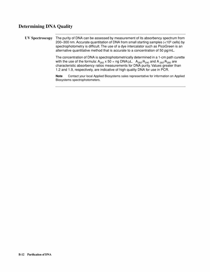
B-12 Purification of DNA
Determining DNA Quality
UV Spectroscopy The purity of DNA can be assessed by measurement of its absorbency spectrum from 200–300 nm. Accurate quantitation of DNA from small starting samples (<105 cells) by spectrophotometry is difficult. The use of a dye intercalator such as PicoGreen is an alternative quantitative method that is accurate to a concentration of 50 pg/mL.
The concentration of DNA is spectrophotometrically determined in a 1-cm path curette with the use of the formula: A260 x 50 = ng DNA/µL. A260/A240 and A
260/A280 are characteristic absorbency ratios measurements for DNA purity. Values greater than 1.2 and 1.9, respectively, are indicative of high quality DNA for use in PCR.
Note Contact your local Applied Biosystems sales representative for information on Applied Biosystems spectrophotometers.
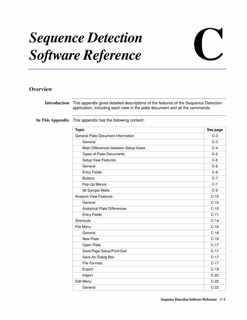
Sequence Detection Software Reference C-1
Sequence Detection Software Reference C
Overview
Introduction This appendix gives detailed descriptions of the features of the Sequence Detection application, including each view in the plate document and all the commands.
In This Appendix This appendix has the following content:
Topic See page
General Plate Document Information C-3
General C-3
Main Differences between Setup Views C-4
Types of Plate Documents C-5
Setup View Features C-6
General C-6
Entry Fields C-6
Buttons C-7
Pop-Up Menus C-7
96 Sample Wells C-9
Analysis View Features C-10
General C-10
Analytical Plate Differences C-10
Entry Fields C-11
Shortcuts C-14
File Menu C-16
General C-16
New Plate C-16
Open Plate C-17
Save/Page Setup/Print/Quit C-17
Save As Dialog Box C-17
File Formats C-17
Export C-18
Import C-20
Edit Menu C-22
General C-22
C

C-2 Sequence Detection Software Reference
Undo/Cut/Copy/Paste/Clear/Select All C-22
Preferences C-22
Setup Menu 24C-
General C-24
Setting Up Thermal Cycler Conditions C-24
Editing a Method. C-26
Sample Type Palette C-33
Sample Type Setup Dialog Box C-33
Editing Sample Attributes C-34
The Sample List C-36
Sample Types/Plate Types. C-37
Adding Sample List Information C-38
Guidelines for IPC C-39
Instrument Menu C-40
General C-40
Run C-40
Stop C-40
Calibrate C-40
Diagnostics C-43
Functions Test C-45
Instrument Verification C-47
Analysis Menu C-48
Purpose of Menu C-48
Display C-48
Options C-49
Statistics/Allele Settings C-49
Allelic Discrimination C-50
Amplification Plot C-52
Multicomponent C-54
Raw Spectra. C-55
Standard Curve C-57
Graph Features C-59
General C-59
Changing Spectra Displayed C-59
Changing Graph Display Features C-60
Windows Menu C-62
General C-62
Experiment Report C-62
Event Log C-63
Topic See page
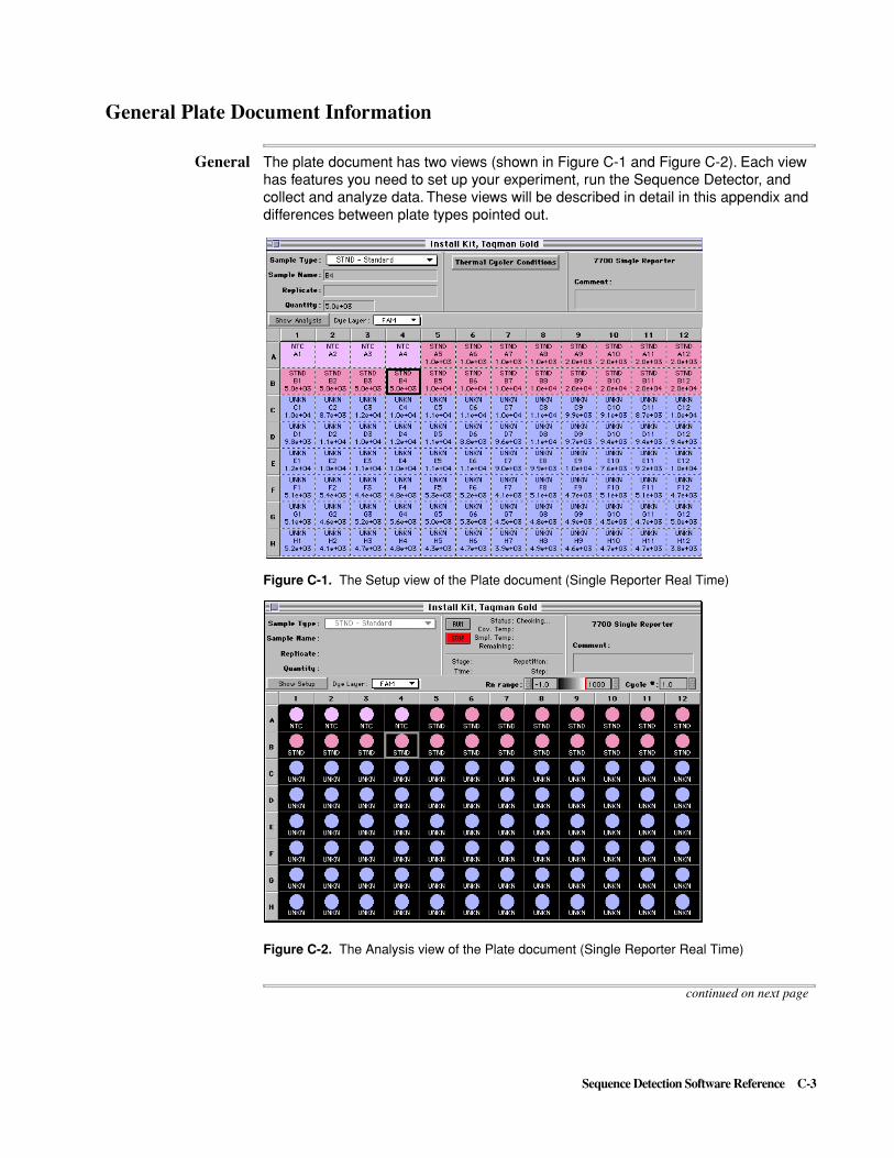
Sequence Detection Software Reference C-3
General Plate Document Information
General The plate document has two views (shown in Figure C-1 and Figure C-2). Each view has features you need to set up your experiment, run the Sequence Detector, and collect and analyze data. These views will be described in detail in this appendix and differences between plate types pointed out.
Figure C-1. The Setup view of the Plate document (Single Reporter Real Time)
Figure C-2. The Analysis view of the Plate document (Single Reporter Real Time)
continued on next page

C-4 Sequence Detection Software Reference
Main Differencesbetween Setup Views
Although both plate views (Setup and Analysis) differ for types of analysis plates, differences between Setup views are easier to explain. Figure C-3 and Figure C-4 illustrate the main differences between Setup views of the analytical plate documents.
Differences in the Analysis view of the different plate types will be discussed in the detailed description of the Analysis view.
Figure C-3. Dye Layer Pop-up on Single Reporter Setup View
The main differences between the Single Reporter Real Time (SRRT) setup view (shown in Figure C-1) and the Allelic Discrimination (AD) setup view (shown in Figure C-4) is that the SRRT setup view has a quantity entry field and multiple dye layers while the AD setup view does not. Any discussion of the dye layers and the dye pop-up menu do not apply to the Allelic Discrimination plate type. The Single Reporter Read Only plate (not shown) is a mixture of both plate types since it does not have a quantity field but does have multiple dye layers.
Figure C-4. Differences in the Setup view for the Allelic Discrimination plate
continued on next page
Dye layer pop-up

Sequence Detection Software Reference C-5
Types of PlateDocuments
There are four types of plate documents which may be opened, Two of these, Background and Pure Spectra, are used in setting up the instrument but not for general operation (see “Background Calibration” on page 3-7 and “Pure Dye Spectra Calibration” on page 3-9 for more information on using these types of plates.
The two types of plates used for analysis are the Allelic Discrimination plate and the Single Reporter plate. This appendix will point out the differences in the interfaces between these types of plates. For information on using these plate types for different applications, see Chapter 3, “Setup and Operation for Real Time Quantitation,” Chapter 4, “Setup and Operation for Allelic Discrimination” and Chapter 5, “Setup and Operation for Plus/Minus Scoring.”

C-6 Sequence Detection Software Reference
Setup View Features
General As Figure C-5 shows, the Setup view contains:
� Entry fields for sample information and comments
� Buttons for entering/displaying the Thermal Cycler Conditions and toggling the view
� Pop-up menus for Dye layers and Sample Types
� 96 sample wells
Figure C-5. Setup View for the Single Reporter Plate for Real Time Quantitation
Entry Fields The Setup view contains three entry fields: Sample Name, Replicate, and Comments. The sample being described may be any sample type. You may use a field to describe the contents of one well or many sample wells selected together. These three fields can hold up to 255 characters each.
Sample Name. Enter a number or text that identifies the sample.
Replicates. A replicate is a way to group samples. Select the wells that you would like to group and then enter a number or text in the Replicate field.
During data analysis, the Sequence Detection application calculates the mean and the Standard Deviation of the replicate group. The Experiment Report displays these replicate values.
Quantity. Enter a number that represents the quantity of the standard sample types. The number you enter is automatically converted to scientific notation.
The Quantity entry field is open for entry only when wells are designated as STND (Standard).
Sample information
View toggle
96 sample wells
Commentfield
Sample Type pop-up
Thermal Cycler Conditions buttonDye layer pop-up

Sequence Detection Software Reference C-7
In scientific notation, the exponential factor is converted to the term “e+”. For example, 1000, which can be represented as 103, becomes 1.0 e+03 in scientific notation.
IMPORTANT Do not type commas in the Quantity entry field.
The same unit of quantity is assigned to all wells on any one plate document. You can determine the default unit assigned to quantity in the Preferences dialog box (page C-22).
Comments. The Comments entry field, on the top right side of the Setup view, holds up to 255 characters. The contents of this entry field also appear on the Analysis view and the Experiment Report. You can edit the comments field in either the Setup view or the Analysis view. Comments entered in this field are presented on the Experiment Report.
Buttons Thermal Cycler Conditions
Click the Thermal Cycler Conditions button to open the Thermal Cycler Conditions dialog box. See page C-24 for more information about Thermal Cycler Conditions.
View Toggle
Click the Show Analysis button to see the Analysis view of the plate document.
Click the Show Setup button to return to the Setup view of the plate document.
Pop-Up Menus The following pop-up menus are provided in a plate document.
Dye Layer.
Click the Dye Layer pop-up menu to look at another dye layer in the plate document. The plate document may have up to eight dye layers.
Note The Dye Layer pop-up menu is not available in Allelic Discrimination type plates.
You can change the contents of the Dye Layer pop-up menu by removing or adding dyes.
� To remove a dye from the Dye Layer pop-up menu, see page C-42.
Number As Exponent In Scientific Notation
1000 103 1.0e+03
2000 2 x 10³ 2.0e+03
5000 5 x 10³ 5.0e+03
10000 104 1.0e+04
20000 2 x 10⁴ 2.0e+04

C-8 Sequence Detection Software Reference
� To add a dye to the Dye Layer pop-up menu, proceed as follows:
Sample Type.
Use the Sample Type pop-up menu to assign a sample type to a selected well or group of wells.The items that appear in the Sample Type pop-up menu vary according to the dye layer you are viewing. For example, when you are looking at the FAM dye layer, you only see sample types that have been labeled with FAM as the Reporter dye in the Sample Type Setup dialog box.
Figure C-6. Sample Pop-up Menus for the three plate types
See page C-33 for information on the Sample Type Setup dialog box.
Step Action
1 Choose Calibrate in the Instrument menu, then choose Setup Pure Spectra.
The Setup Pure Spectra dialog box opens.
2 Click the Show All button.
All available pure spectra now appear in the dialog box.
3 Is the dye you want to add to the Dye Layer pop-up menu available?If no, perform a Pure Dye Spectra calibration of the dye. See “Pure Dye Spec-
tra Calibration” on page 3-9 for the Pure Dye Spectra Calibration proce-dure. Then return to step 1 of this procedure.
If yes, continue to step 4.
4 Check the checkbox next to the dye to make it an active dye.
5 Click OK to close the dialog box.
The Dye Layer pop-up menu now contains the new active dye.
Single Reporter Allelic Discrimination Pure Spectra(FAM layer) (not layer dependent) (not layer dependent)
Pure Spectra Calibration

Sequence Detection Software Reference C-9
To assign a sample to one or more wells with the Sample Type pop-up:
96 Sample Wells Figure C-7 illustrates the labeling of wells on a simulated 96-well plate: “1–12” horizontally, across the top of the plate, and “A–H” vertically, on the left side of the plate. Each of the 96 wells has a unique label combining the vertical and horizontal labels, such as A1, C4, F10, and G12 which appear on the Experiment Report and graphs of data.
Figure C-7. Examples of information displayed in wells
On the Setup view, each well can display three lines of information. The top line displays the Sample Type you selected from either the Sample Type pop-up menu or the Sample Type Palette. The middle line displays either the well label or the information in the Sample Name field. The bottom line displays the information in the Quantity field.
To select wells on a plate document:
� To select multiple contiguous wells, hold down the mouse button as you click and drag the cursor across the plate.
Figure C-8. Selecting multiple contiguous wells
� To select multiple discontinuous wells, hold down the Command (c) key and click on wells.
� To select an entire row or column of wells, click on a row or column label (A–H, 1–12).
Selected wells are outlined in black.
Step Action
1 Select one or more wells that contain the same sample.
2 Click the Sample Type pop-up menu and select a sample type.
� Select Edit Sample List to open the Sample Type Setup dialog box.
� Select Not in Use to delete sample information in a selected dye layer and well
Sample TypeWell label
Sample TypeSample NameQuantity
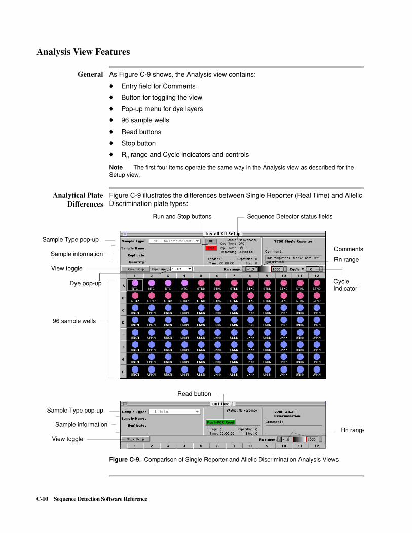
C-10 Sequence Detection Software Reference
Analysis View Features
General As Figure C-9 shows, the Analysis view contains:
� Entry field for Comments
� Button for toggling the view
� Pop-up menu for dye layers
� 96 sample wells
� Read buttons
� Stop button
� Rn range and Cycle indicators and controls
Note The first four items operate the same way in the Analysis view as described for the Setup view.
Analytical PlateDifferences
Figure C-9 illustrates the differences between Single Reporter (Real Time) and Allelic Discrimination plate types:
Figure C-9. Comparison of Single Reporter and Allelic Discrimination Analysis Views
Sample information
View toggle
96 sample wells
Sample Type pop-up
Sequence Detector status fieldsRun and Stop buttons
Comments
Rn range
Dye pop-up
Sample information
Sample Type pop-up
View toggle
Read button
Rn range
CycleIndicator

Sequence Detection Software Reference C-11
Entry Fields The information entered on the Setup view in the sample information and comments appears on the Analysis view. This information can also be edited in the Analysis view.
Run and Stop Buttons
The Sequence Detector is ready to run when:
� All the parameters of the experiment have been defined on the Setup view
� The 96-well plate has been placed on the sample block, and
� The cover of the sample block has been tightened.
To run the Sequence Detector:
� Click the Run button on the Analysis view of the plate document or use the keyboard shortcut, Cmd R.
As the Sequence Detector starts the run, the adjoining Status field flashes the word Success, followed by the word Waiting.
The Sequence Detector does not begin running until the temperature of the sample block cover reaches 105 °C. The adjoining Status field flashes the word Ramping as the temperature of the sample block increases.
To stop the sequence detector:
� Click the Stop button.
If you are stopping a run before it has completed all the Stages defined in the Thermal Cycler Conditions, a dialog box opens when you click the Stop button.
Figure C-10. Data Handling dialog box
Use this dialog box to either save or discard the data already acquired.
To handle acquired data before stopping a run:
Data handling options
Step Action
1 Select one of the two data handling options.
2 Click OK to abort the run. Click Cancel to continue the run and collect more data
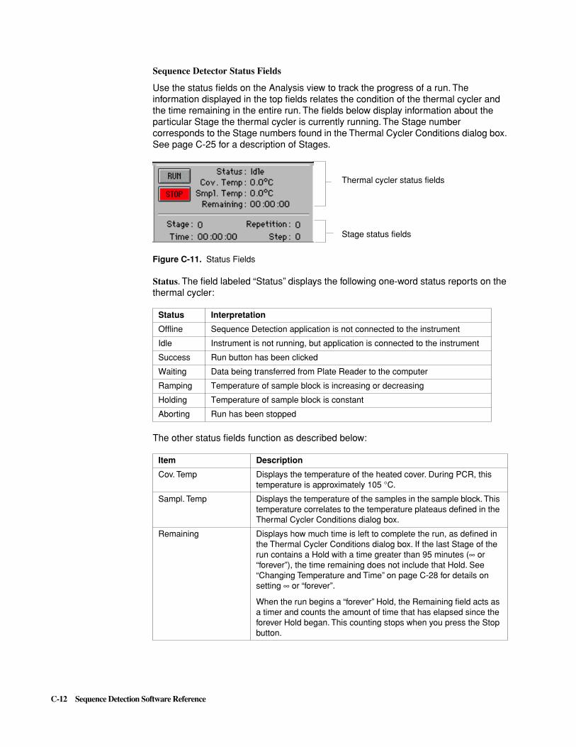
C-12 Sequence Detection Software Reference
Sequence Detector Status Fields
Use the status fields on the Analysis view to track the progress of a run. The information displayed in the top fields relates the condition of the thermal cycler and the time remaining in the entire run. The fields below display information about the particular Stage the thermal cycler is currently running. The Stage number corresponds to the Stage numbers found in the Thermal Cycler Conditions dialog box. See page C-25 for a description of Stages.
Figure C-11. Status Fields
Status. The field labeled “Status” displays the following one-word status reports on the thermal cycler:
The other status fields function as described below:
Status Interpretation
Offline Sequence Detection application is not connected to the instrument
Idle Instrument is not running, but application is connected to the instrument
Success Run button has been clicked
Waiting Data being transferred from Plate Reader to the computer
Ramping Temperature of sample block is increasing or decreasing
Holding Temperature of sample block is constant
Aborting Run has been stopped
Item Description
Cov. Temp Displays the temperature of the heated cover. During PCR, this temperature is approximately 105 °C.
Sampl. Temp Displays the temperature of the samples in the sample block. This temperature correlates to the temperature plateaus defined in the Thermal Cycler Conditions dialog box.
Remaining Displays how much time is left to complete the run, as defined in the Thermal Cycler Conditions dialog box. If the last Stage of the run contains a Hold with a time greater than 95 minutes (• or “forever”), the time remaining does not include that Hold. See “Changing Temperature and Time” on page C-28 for details on setting • or “forever”.
When the run begins a “forever” Hold, the Remaining field acts as a timer and counts the amount of time that has elapsed since the forever Hold began. This counting stops when you press the Stop button.
Thermal cycler status fields
Stage status fields
Sequence Detection Software Reference C-13
Stage Displays the number of the Stage of the run currently being performed. The Stage numbers correspond to the Stage numbers that appear in the Thermal Cycler Conditions dialog box. See page for a discussion of Stages.
Time Displays the time remaining until the end of the Stage.
Repetition Counts the number of cycle repetitions that have been performed during one Stage. During a Hold, no numbers appear in this field.
Step Displays the number of the Step currently being performed. In a typical two-step Cycle of one melting step followed by an anneal-extension step, the Step number is 1 during a melting step and 2 during anneal-extension.
Item Description
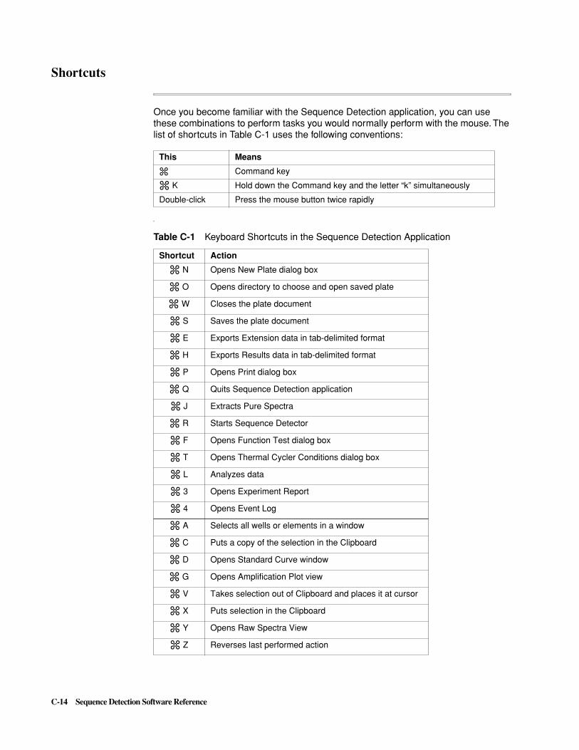
C-14 Sequence Detection Software Reference
Shortcuts
Once you become familiar with the Sequence Detection application, you can use these combinations to perform tasks you would normally perform with the mouse. The list of shortcuts in Table C-1 uses the following conventions:
n
This Means
c Command key
c K Hold down the Command key and the letter “k” simultaneously
Double-click Press the mouse button twice rapidly
Table C-1 Keyboard Shortcuts in the Sequence Detection Application
Shortcut Action
c N Opens New Plate dialog box
c O Opens directory to choose and open saved plate
c W Closes the plate document
c S Saves the plate document
c E Exports Extension data in tab-delimited format
c H Exports Results data in tab-delimited format
c P Opens Print dialog box
c Q Quits Sequence Detection application
c J Extracts Pure Spectra
c R Starts Sequence Detector
c F Opens Function Test dialog box
c T Opens Thermal Cycler Conditions dialog box
c L Analyzes data
c 3 Opens Experiment Report
c 4 Opens Event Log
c A Selects all wells or elements in a window
c C Puts a copy of the selection in the Clipboard
c D Opens Standard Curve window
c G Opens Amplification Plot view
c V Takes selection out of Clipboard and places it at cursor
c X Puts selection in the Clipboard
c Y Opens Raw Spectra View
c Z Reverses last performed action
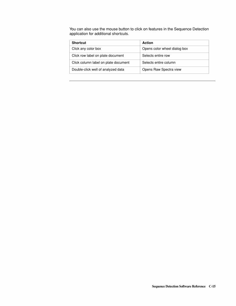
Sequence Detection Software Reference C-15
You can also use the mouse button to click on features in the Sequence Detection application for additional shortcuts.
Shortcut Action
Click any color box Opens color wheel dialog box
Click row label on plate document Selects entire row
Click column label on plate document Selects entire column
Double-click well of analyzed data Opens Raw Spectra view

C-16 Sequence Detection Software Reference
File Menu
General All experiments you setup and run with the Sequence Detection application use a plate document to display sample wells and their associated data. Use the commands in the File menu to open, save and close plate documents, input format or setup files, export collected data, and handle printing tasks.
NewPlate
General
Opens a new plate document.
Figure C-12. New Plate dialog box
The New Plate dialog box contains three pop-up menus, labeled “Plate Type,” “Instrument,” and “Run.” The terms on the dialog box are described in the table below:
Data Acquisition
Data acquisition is controlled by choices made for the following two parameters:
Instrument. The software supports two instruments, the 7200 and the 7700. Choose the “7700 Sequence Detector” for the present instrument.
Run. Two types of data acquisition runs are available: Real Time, which collects data at every cycle of the PCR; and Plate Read, which collects only one set of data after PCR is complete.
continued on next page
Item Description
Plate Type Four plate types are available, corresponding to the types of plates you need to run experiments on the instrument: Single Reporter, Allelic Discrimination, Background and Pure Spectra.
Single Reporter Use this plate type when all probes in your experiment are labeled with the same reporter, either with or without an IPC layer.
Allelic Discrimination Use this plate type to run an experiment that distinguishes between two alleles.
Background Use this plate type to generate a background component (see page C-40 and page 3-7).
Pure Spectra Use this plate to generate pure dye components (see page C-41 and page 3-10).

Sequence Detection Software Reference C-17
Open Plate Opens a plate document that has previously been used and saved.
Save/PageSetup/Print/Quit
These commands have the normal Macintosh computer functions. Only commands which differ in some way from those on a standard File menu are discussed.
Save As Dialog Box Assigns a name and file format while saving the active plate document. A plate document can be saved in either Normal or Stationery file format.
Figure C-13. Save As dialog box1
File Formats Normal File Format
A plate document saved in normal file format contains the following information:
� Sample types in each well
� All information in the Thermal Cycler Conditions dialog box
If you save a plate document in normal file format after PCR data has been collected, the saved document also contains:
� All collected data, but without analyzed data
� Background and pure spectra components
Stationery File Format
A plate document saved in stationery file format contains:
� Sample types in each well
� All information in the Thermal Cycler Conditions dialog box
You can save plate documents as stationery files for those experiments that you plan to repeat frequently. When you open a stationery file, the Sequence Detection application opens a copy of the file for you to use. Changes you make to the copy do not affect the original stationery plate file. When you save or close the copy, you can save it as a normal file or re-name it as another stationery file. The Sequence Detection application labels stationery plate files with a unique icon.
continued on next page

C-18 Sequence Detection Software Reference
Export You can export raw or analyzed data in tab-delimited format for all 96 wells or for a selected group of wells on a plate. You can open these exported files with any application that reads tab-delimited text.
Exported data files contain records of temperature changes and relevant data collected at each designated data collection point. Table C-2 describes specific data collected for each export option. A spectral bin represents a portion of the complete range of measured wavelength, from approximately 500–660 nm.
Table C-2 Exported Data Options
Export Option ProducesData vs. Plate Type(RT PR AD)
Raw Spectra One unique data file for each well selected. Contains data collected at each of 32 spectral bins throughout all Stages of PCR that have been labeled with Data Collection icons in the Thermal Cycler Conditions dialog box. A data point is collected approximately once every 7 seconds.
X X X
Pure Spectra Pure dye component data, one data point for each of 32 spectral bins, and 96 wells of background data for each spectral bin.
X N/A N/A
Multicomponent The calculated amount of each dye component in any well throughout all Stages of PCR that have been labeled with Data Collection icons in the Thermal Cycler Conditions dialog box. A data point is collected approximately once every 7 seconds. Also contains pure spectra component data, the calculated inverse matrix, and single values of the inverse matrix.
X X X
Clipped The average of the last 3 data points collected during the extension phase of each cycle repetition for each selected well.
X N/A N/A
Extension One extension step data point for each of 32 spectral bins, at each cycle repetition, for each well.
X N/A N/A
Results For a Real Time run, results include Ct, Quantity, and Mean (except NTCs), and Standard Deviation for replicates for each well selected. The only data for NTCs is Ct.
Other Real Time data includes Standard Curve information such as slope, intercept, fit, threshold, and baseline range.
For a Plate Read run, results include data at a single end point for each well. A Single reporter type Plate Read provides Rn and DRn at end point and +/- detection of template. An Allelic Discrimination type Plate Read provides allele calls for each sample (Allele 1 homozygous, Allele 2 homozygous, or Allele 3 heterozygous).
X X

Sequence Detection Software Reference C-19
To export data in tab-delimited format:
continued on next page
Step Action
1 Select the entire plate (click upper left corner of well area) to select all wells or select a group of wells and then choose Export in the File menu and choose the type of data to export.
Note After analysis the full range of choices shown to the right above are available for export.
2 Then choose the type of data to export.
3 Indicate where the data file should be stored and type the file name in the entry field.
4 Export All Wells is available as a default, allowing you to export the data from all 96 wells. Select Export Selected Wells if you want to export data only from wells you selected in step 1.
5 Click Export to complete data export.
Export choices before analysis
Export choices after analysis
Selected by defaultClick to export raw spectra data fora selected group of wells.
This is the signal from the detectionsystem with no light input.
(AmpliTaq Gold™)

C-20 Sequence Detection Software Reference
Import As shown in the dialog box below, this command is used to import either of two types of file setup information after you have opened a new plate. Use the “Import Lab View Format File” option to import a new Experiment Report format created in the Lab View application. Use the “Import Setup File” option to import a Setup File you have prepared.
Figure C-14. Import dialog box
The ABI PRISM 7700 system can import a Setup file. A Setup file allows you to electronically transfer position, sample type, and sample name from a tab-delimited text file into your plate document. The major benefit of this feature is the ability to transfer existing sample names into a new plate document without retyping, as shown in Figure C-15.
Figure C-15. Example of a Setup file
7

Sequence Detection Software Reference C-21
The tab-delimited text file (which can be created in programs such as Word and Excel) must contain the following information:
� Position —this can be entered as a number (1-96) or the well position (A1-H12).
� Sample Type —you must enter the exact acronym as shown in the Sample Type setup of the plate you are importing into. (You can always label all your samples as UNKN and then modify the Sample Type later.)
� Sample Name — any alphanumeric name up to 255 characters.
Note Columns 1 (Position) and Column 2 (Sample Type Acronym) are required and Columns 3 and 4 (Sample Name and Quantity or amount) are optional.
Figure C-16. Choosing a file to import
To import a Setup file, follow this procedure:
Step Action
1 From the File menu, choose New Plate.
2 From the File menu, choose the Import Setup file command.
3 In the dialog box that appears, choose the file to import.

C-22 Sequence Detection Software Reference
Edit Menu
General Use the commands in the Edit menu to modify text and graphical elements in the plate document. You cannot use commands in the Edit menu to modify data. Use the Preferences in the Edit menu to define default parameters, such as the quencher and passive reference dyes.
Some commands in the Edit menu use the Clipboard on your Macintosh computer. For more information on the Clipboard, see the Macintosh Guide, an on-line help file distributed with all Macintosh computers.
Undo/Cut/Copy/Paste/Clear/
Select All
These commands have the normal Macintosh functions. Only commands which differ in some way from those on a standard File menu are discussed.
Preferences The features you choose in Preferences are applied by default to every new plate you open.
Figure C-17. Preferences dialog box
IMPORTANT After you make changes to the Preferences, you must close the plate document that is currently open and re-open it to apply the new Preferences.
New Document Defaults.
Offers the same options displayed in the New Plate dialog box. These options are applied to the plate document that automatically opens when you open the Sequence Detection application. The choices available in the dialog box are described below:
Item Description
Plate “types” With the next parameter, Instrument, set to “7700 Sequence Detector,” the choices are Single Reporter, Allelic Discrimination, Background, or Pure Spectra. For descriptions of Plate Types, see “New Plate” on page C-16. The Background and Pure Spectra plates are used to generate these types of data when setting the instrument up or when re-generating these types of data files (see “Background Calibration” on page 3-7 and “Pure Dye Spectra Calibration” on page 3-9).
Instrument “types” From the Instrument pop-up, choose “7700 Sequence Detector” as the sequence detection system you are using with the Sequence Detection application, enabling either real-time or plate read Run types:
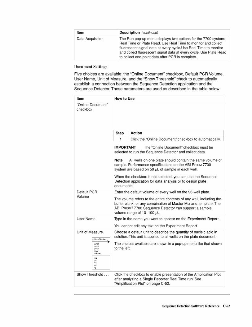
Sequence Detection Software Reference C-23
Document Settings
Five choices are available: the “Online Document” checkbox, Default PCR Volume, User Name, Unit of Measure, and the “Show Threshold” check to automatically establish a connection between the Sequence Detection application and the Sequence Detector. These parameters are used as described in the table below:
Data Acquisition The Run pop-up menu displays two options for the 7700 system: Real Time or Plate Read. Use Real Time to monitor and collect fluorescent signal data at every cycle.Use Real Time to monitor and collect fluorescent signal data at every cycle. Use Plate Read to collect end-point data after PCR is complete.
Item How to Use
“Online Document” checkbox
IMPORTANT The “Online Document” checkbox must be selected to run the Sequence Detector and collect data.
Note All wells on one plate should contain the same volume of sample. Performance specifications on the ABI PRISM 7700 system are based on 50 µL of sample in each well.
When the checkbox is not selected, you can use the Sequence Detection application for data analysis or to design plate documents.
Default PCR Volume
Enter the default volume of every well on the 96-well plate.
The volume refers to the entire contents of any well, including the buffer blank, or any combination of Master Mix and template. The ABI PRISM® 7700 Sequence Detector can support a sample volume range of 10–100 µL.
User Name Type in the name you want to appear on the Experiment Report.
You cannot edit any text on the Experiment Report.
Unit of Measure. Choose a default unit to describe the quantity of nucleic acid in solution. This unit is applied to all wells on the plate document.
The choices available are shown in a pop-up menu like that shown to the left.
Show Threshold . . . Click the checkbox to enable presentation of the Amplication Plot after analyzing a Single Reporter Real Time run. See "Amplification Plot" on page C-52.
Item Description (continued)
Step Action
1 Click the “Online Document” checkbox to automatically

C-24 Sequence Detection Software Reference
Setup Menu
General Use the commands in the Setup menu with the Setup view of the plate document to define your samples and assign sample types to wells.
Setting Up ThermalCycler Conditions
Two Views
The Thermal Cycler Conditions dialog box contains two view s (Figure C-18, one view for defining the method, the second view for defining data collection points.
Figure C-18. Thermal Cycler Conditions contains two views
A method (defined by the upper Thermal Cycler Conditions view) contains all the information about time and temperature changes that occur during a complete thermal
To change views, click Show Data Collection
To change views, click Show Time and Temperature

Sequence Detection Software Reference C-25
cycle run. The Time and Temperature view (shown immediately above) displays a graphic representation of a method (see Figure C-19).
Figure C-19. A graphic representation of a method
Stages.
A Stage is one division of a method; a Stage can be either a Hold or a Cycle. The method shown in Figure C-19 consists of three Stages: two Holds, followed by a Cycle. Vertical lines mark where one Stage ends and the next Stage begins.
During PCR on the ABI PRISM 7700 Sequence Detector, the Analysis view of the plate document tracks the progress of the reaction and displays the number of the Stage that is currently running (page C-12).
Holds, Cycles, and Steps.
A Step is a temperature plateau preceded by a ramp. In Figure C-19, a ramp is represented by a slanting line that connects two temperature plateaus. By default, each ramp represents the shortest amount of time needed to go from one temperature plateau to the next.
A Hold contains one or more Steps that are performed only once. During the Hold in Stage1 in Figure C-19, UNG digestion of amplified DNA occurs at 50 °C, followed by a Hold in Stage 2, a denaturation of nuclear material at 95 °C. The final Hold, in Stage 4, is a cooling step for storing samples.
A Cycle contains two or more Steps that are repeated numerous times within a method. The Cycle shown in Stage 3 in Figure C-19 is repeated 40 times. A typical two-temperature cycle for PCR with TaqMan probes consists of a denaturation, or melting, step at 95 °C for 15 sec, followed by an anneal-extension step at 60 °C for 1 minute.
continued on next page
Number of cycle repetitions
Ramp
TemperatureTime

C-26 Sequence Detection Software Reference
Editing a Method. There are several ways to edit the features in a method. You can:
� Add or remove Steps, Cycles, or Holds
� Change the temperature or time associated with any Step
� Adjust the ramp time between two Steps
� Define an Auto Increment for time and temperature
Adding to a Method with Insert Bars
To add a Step, Cycle or Hold, you must click a step to bring up an Insert bar. the Insert bar appears as a thick vertical line at either the end or the beginning of a selected Step. A selected Step appears as a colored line.
Note You cannot add a Step, Cycle, or Hold after a step with a time greater than 89:59 minutes (•).
To add a Step, Cycle, or Hold:
Table C-3 shows the default temperatures and times assigned to new Steps, Cycles, and Holds.
Step‘ Action
1 Click the Thermal Cycler Conditions button to display the current method.
2 Click on a Step.
An Insert bar appears either at the end or at the beginning of the selected Step. Click on one side or the other of the Insert bar to determine its relative position.
3 Do one of the following to add to a method:
� Click the appropriate button to add a new Step, Cycler, or Hold.
� Click the Add Step button to add a new Step.
� Click the Add Cycle button to add a new Cycle.
� Click the Add Hold button to add a new Hold.
Insert bar

Sequence Detection Software Reference C-27
Where the new Step, Cycle or Hold appears depends on whether the Insert bar appears to the right or left of the selected step, as Table C-4 illustrates. A Step inserted in a Hold or Cycle becomes part of that Hold or Cycle.
Note You cannot insert a Hold or Cycle in the middle of a Cycle.
Deleting Items Positioned by Insert Bars
Table C-3 Default Configuration of New Steps, Cycles, and Holds
Step Cycle Hold
Temperature (°C) 54.0 95.0 60.0 50.0
Time (min:sec) 01:00 00:15 01:00 01:00
Table C-4 Placement of New Steps, Cycles and Holds
Location of Insert Bar
Step Hold Cycle
Left of Hold Beginning of Hold Beginning of Hold Beginning of Hold
Right of Hold End of Hold End of Hold End of Hold
Left of Cycle Beginning of Cycle Beginning of Cycle Beginning of Cy-cle
Middle of Cycle Middle of Cycle End of Cycle End of Cycle
Right of Cycle End of Cycle End of Cycle End of Cycle
To delete a Step, Cycle or Hold:
Step Action
1
Click the Thermal Cycler Conditions button in the Setup view to display the current method.
Selected Step

C-28 Sequence Detection Software Reference
Changing Temperature and Time
The temperature range of the sample block is 4.0–99.9 °C. The Sequence Detection application does not permit a temperature greater than 99.9 °C or less than 4 °C in any Temperature field.
The Sequence Detection application collects a full 96-well plate of fluorescence data approximately once every 7 seconds.The application’s algorithm averages the last three data points collected during the extension step and uses that average to represent extension step fluorescence. For best results, the extension step should be at least 30 seconds to allow collection of sufficient data.
Note Do not enter a value less than 30 seconds (00:30) for the extension step, the second Cycle step in a two-step PCR.
Figure C-20. Changing temperature or time
IMPORTANT The Thermal Cycler Conditions window will accept a 4° C hold at the end of thermal cycling. At this time, however, since all real-time data has already been collected at that point and because 4° C holds can cause excessive water condensation in the sample tray area, 4° C holds are usually not needed.
To change the temperature or time associated with a Step:
2 Click on the Step you want to delete. If you want to delete a series of Steps, click on the last Step on the right in the series of Steps.
An Insert bar appears at the end of the temperature plateau.
3 Drag the cursor from the Insert bar to the left across the Step, Cycle, or Hold to select the Steps to be deleted.
4 Drag the cursor from the Insert bar to the left across the Step, Cycle, or Hold to select the Steps to be deleted.
5 In the Edit menu, choose the Clear command.
To delete a Step, Cycle or Hold: (continued)
Step Action
TemperatureTime (minutes:seconds)
Step Action
1 Click in the time or temperature field you wish to change and drag the cursor across the numbers to select them.

Sequence Detection Software Reference C-29
Adjusting Ramp Time
The ramp time between two Steps in the Thermal Cycler Conditions is the time needed to go from one temperature to the next. When the ramp time is set to the minimum ramp time of zero, the rate of temperature change on the thermal cycler is approximately 1 °C/second. For example, the shortest possible time necessary to ramp from 50 °C to 95 °C is approximately 45 seconds. The maximum ramp time is 9 minutes and 59 seconds.
To adjust the ramp time between two Steps:
2 Enter a new value.
A period (.) automatically appears after you enter the first two digits in the Temperature field. A colon (:) automatically appears after you enter the first two digits in the Time field.
� To enter 9 minutes in any Time field, type 09:00.
� To enter a value less than a minute in any time field which already is set to 1 minute or more, do the following:
a) Select the portion of the field after the colon and type in the new value in seconds (5 seconds is the minimum value allowed),
b) then select the two digits before the colon and type “00”.
� To enter a • (forever) time for the last hold, do the following:
a) Select the time field and type 89:59,
b) select the initial 8 and then type 9,
c) then click OK to put an • symbol in the time field.
Note The procedure immediately above is required because you cannot directly enter a value greater than 89:59 in a Time field. After you type the first 9 in the time field, no further entry is allowed unless you proceed as listed above.
3 Press the Tab key to move the cursor to the next field.
Step Action
1 Click the Thermal Cycler Conditions button to display the current method.
2 Click on the Step that contains the ramp time you want to modify. By definition, the ramp precedes the temperature plateau in a Step.
An Insert bar appears at the end of the Step.
3 Click the Set Ramp Time button.
The Ramp Time dialog box appears.
4 Click the up or down arrows to adjust the ramp time.
The adjusted ramp time appears in the box between the pairs of arrows.
Step Action
Ramp Time (min:sec)
Seconds adjustmentMinutes adjustment

C-30 Sequence Detection Software Reference
Auto Incrementing and Decrementing
You can automatically increase or decrease the time or temperature associated with any Step by a fixed amount with each Cycle repetition. For example, you can increase the extension time of a Cycle to accommodate the increased amount of amplicons produced as PCR progresses.
The Auto Increment feature appears in the Thermal Cycler Conditions dialog box. With this feature you can:
� Increase or decrease any time or temperature in a Cycle
� Modify both time and temperature for one or more Steps in a Cycle
IMPORTANT The temperature range of the thermal cycler sample block is 4.0–99.9 °C. The Sequence Detection application does not accept an auto-increment value that would eventually cause the temperature of the sample block to exceed this range.
5 Click the OK button.
The modified ramp time appears on the ramp in the Thermal Cycler Conditions box.
Step Action
Modifiedramp time
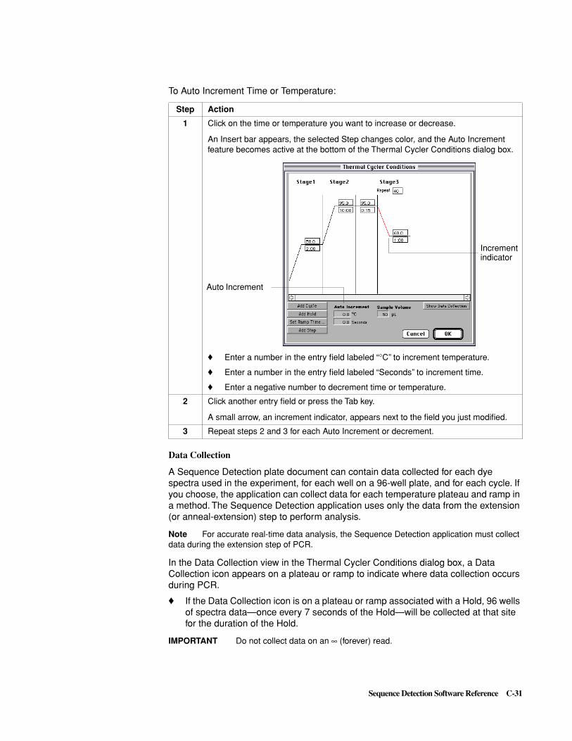
Sequence Detection Software Reference C-31
Data Collection
A Sequence Detection plate document can contain data collected for each dye spectra used in the experiment, for each well on a 96-well plate, and for each cycle. If you choose, the application can collect data for each temperature plateau and ramp in a method. The Sequence Detection application uses only the data from the extension (or anneal-extension) step to perform analysis.
Note For accurate real-time data analysis, the Sequence Detection application must collect data during the extension step of PCR.
In the Data Collection view in the Thermal Cycler Conditions dialog box, a Data Collection icon appears on a plateau or ramp to indicate where data collection occurs during PCR.
� If the Data Collection icon is on a plateau or ramp associated with a Hold, 96 wells of spectra data—once every 7 seconds of the Hold—will be collected at that site for the duration of the Hold.
IMPORTANT Do not collect data on an • (forever) read.
To Auto Increment Time or Temperature:
Step Action
1 Click on the time or temperature you want to increase or decrease.
An Insert bar appears, the selected Step changes color, and the Auto Increment feature becomes active at the bottom of the Thermal Cycler Conditions dialog box.
� Enter a number in the entry field labeled “°C” to increment temperature.
� Enter a number in the entry field labeled “Seconds” to increment time.
� Enter a negative number to decrement time or temperature.
2 Click another entry field or press the Tab key.
A small arrow, an increment indicator, appears next to the field you just modified.
3 Repeat steps 2 and 3 for each Auto Increment or decrement.
Incrementindicator
Auto Increment

C-32 Sequence Detection Software Reference
� If the Data Collection icon is on a plateau or ramp associated with a Cycle, then multiple sets of data spectra, one set for each cycle repetition, will be collected at that site.
The more data collection points there are in a method, the larger the corresponding data file for that run.
Figure C-21. Data Collection Icon
To add or remove a Data Collection icon:
� Click once on a plateau in the Data Collection view to add an icon.
� Click once on a Data Collection icon to remove the icon.
You may remove all Data Collection icons in the Data Collection view if you want to use the ABI PRISM 7700 Sequence Detector for only thermal cycling. The Sequence Detection application does not collect fluorescent data during PCR when the Data Collection view shows no Data Collection icons.
Note When the Data Collection view contains no icons, the Sequence Detection application does not collect data during a run. Also, data is not collected on ramps.
See "Instrument Menu" on page C-40 for more information on how collected data is analyzed.
continued on next page
Data Collection icon

Sequence Detection Software Reference C-33
Sample Type Palette The Sample Type Palette (shown on the left below) is a floating window that displays all the Sample Types you can assign to the wells on the plate document. You can move a floating window around on the monitor screen. To use the Sample Type Palette to assign samples to wells, see page 3-17.
Every Sample Type that appears in the Sample Type Setup also appears in the Sample Type Palette. If you want more sample types on the Sample Type Palette, you must edit the Sample Type Setup.
Figure C-22. Sample Type Palette
Note The Sample Type Palette allows you to set up and view multiple dye layers for the selected wells.
To edit the list of samples on the Sample Type Palette:
� Click the Edit Sample List button.
The Sample Type Setup dialog box opens. Modify the list of samples in the Sample Type Setup dialog box to change the list of samples in the Sample Type Palette. See page C-38.
Sample Type SetupDialog Box
The Sample Type Setup dialog box displays each item in the Sample List with its associated Acronym, Name, Color and Reporter. In this dialog box, you can add or remove samples or edit the sample’s attributes.
Figure C-23. Sample Type Setup dialog box
continued on next page
Click here toEdit Sample List

C-34 Sequence Detection Software Reference
Editing SampleAttributes
Acronym and Name
The sample’s Acronym appears in several locations in the Sequence Detection application program: on the Sample Type Palette, across the top of the wells on the plate document, and in the Type column on the Experiment Report. It can hold a maximum of 6 characters.
To successfully import a setup file, the setup file must use an identical acronym to those present in the Sample type setup of the target plate document.
The sample’s Name can be more descriptive than its Acronym and contains up to 64 characters.
To change the sample Acronym or Name, follow this procedure:
Color
The sample’s Color appears on the plate document, applied to the wells that contain the sample. To change the sample Color, follow this procedure:
Reporter and Quencher
The reporter dye attached to the fluorogenic probe that specifically anneals with the sample. A sample’s Reporter is changed as described in the procedure on the next page.
Note All dye pop-up menus display only the dyes that are active. See page C-42 for a discussion of active dyes.
Designate the one Quencher dye attached to all fluorogenic probes on one plate. TAMRA is the default Quencher dye.
Step Action
1 Select the Name or Acronym and type the change in the entry field.
2 Click OK to close the Sample Type Setup dialog box
Step Action
1 Double-click the sample’s color in the Sample Type Setup dialog box.
A dialog box displays a color wheel.
2 Choose a new color for the sample and click OK.
3 Click OK to close the Sample Type Setup dialog box.

Sequence Detection Software Reference C-35
Note For proper analysis of a Single Reporter Plate type, you must use UNKN and NTC sample types. For proper analysis of a Allelic Discrimination Plate type, you must use AL1, AL2, and NTC sample types. If these acronyms are not present, analysis will not work properly.
To change the associated Reporter or Quencher dye, follow this procedure:
Note If you change the reporter dye for NPC from FAM to JOE, NPC will no longer be present on the FAM layer in the Sample Type pop-up menu but will now be present in the Sample Type pop-up menu on the JOE layer.
Reference
The passive reference dye that is added to all samples on the plate to normalize reporter signal. ROX is always used as the Reference dye.
Note You cannot edit the Acronyms or Names of the first two entries in the sample list, STND or UNKN.
You cannot directly modify the lists in the Sample Type Palette or in the Sample Type pop-up menu. You must modify them indirectly, by making changes in the Sample Type Setup dialog box.
continued on next page
Step Action
1
Choose the appropriate dye for the Reporter or Quencher from the pop-up menu.
2 Click OK to close the Sample Type Setup dialog box.
Reporter pop-up menu
Quencher pop-up menu
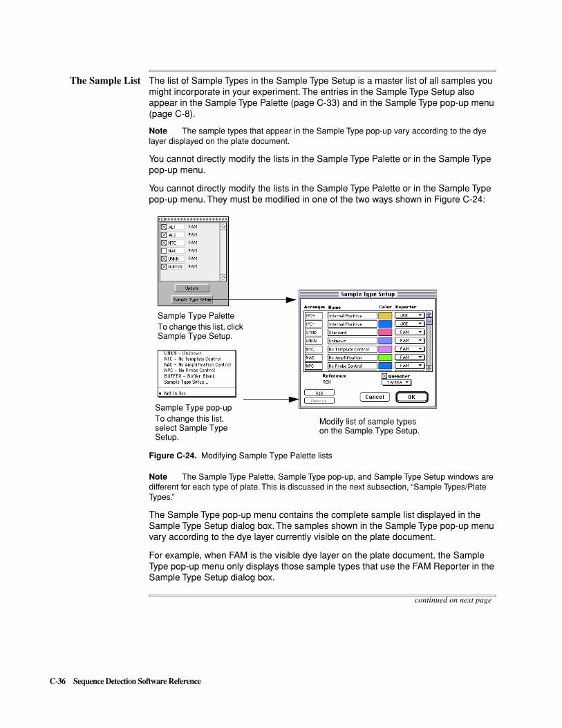
C-36 Sequence Detection Software Reference
The Sample List The list of Sample Types in the Sample Type Setup is a master list of all samples you might incorporate in your experiment. The entries in the Sample Type Setup also appear in the Sample Type Palette (page C-33) and in the Sample Type pop-up menu (page C-8).
Note The sample types that appear in the Sample Type pop-up vary according to the dye layer displayed on the plate document.
You cannot directly modify the lists in the Sample Type Palette or in the Sample Type pop-up menu.
You cannot directly modify the lists in the Sample Type Palette or in the Sample Type pop-up menu. They must be modified in one of the two ways shown in Figure C-24:
Figure C-24. Modifying Sample Type Palette lists
Note The Sample Type Palette, Sample Type pop-up, and Sample Type Setup windows are different for each type of plate. This is discussed in the next subsection, “Sample Types/Plate Types.”
The Sample Type pop-up menu contains the complete sample list displayed in the Sample Type Setup dialog box. The samples shown in the Sample Type pop-up menu vary according to the dye layer currently visible on the plate document.
For example, when FAM is the visible dye layer on the plate document, the Sample Type pop-up menu only displays those sample types that use the FAM Reporter in the Sample Type Setup dialog box.
continued on next page
Sample Type PaletteTo change this list, click Sample Type Setup.
Sample Type pop-upTo change this list, select Sample Type Setup.
Modify list of sample types on the Sample Type Setup.

Sequence Detection Software Reference C-37
Sample Types/PlateTypes.
The sample types available and required for each plate type are listed in Table C-5.
The Sample List can hold over 50 entries. You can customize the list so that the entries match the samples you use in your experiment. You cannot remove STND or UNKN, the first two entries on the Sample List.
continued on next page
Table C-5 Sample Types for Each Plate Type
Plate Types Default Sample Types Minimum Setup Required for Analysis
Pure Dye Spectra � At least one tube of FAM
� At least one tube of TET
� At least one tube of TAMRA
� At least one tube of ROX
We suggest using four tubes for each dye.
Single Reporter � At least eight tubes of NTC
All the rest of your samples can be designated as UNKNs.
Single Reporter with IPC
The default sample types are the same as shown above. You must add an IPC+ and IPC- sample type (or use the Stationery file provided).
On the target layer:
� At least eight tubes of NTC
All the rest of your samples can be designated as UNKNs.
On the IPC layer:
� At least eight tubes of IPC-
All the rest of your samples can be designated as IPC+
Allelic Discrimination
� Eight tubes of AL1
� Eight tubes of AL2
� Eight tubes of NTCs
All of the rest of your samples can be designated as UNKN.

C-38 Sequence Detection Software Reference
Adding Sample ListInformation
The following procedures are provided:
� A procedure for adding a sample to the Sample Type Setup
� A procedure for removing a sample from the Sample Type Setup
� Guidelines for IPC/starting with the appropriate Stationery file for your assay (the next subsection)
Adding a Sample
To add a sample to the Sample Type Setup, follow this procedure:
Removing a Sample
To remove a sample in the Sample List, follow this procedure:
continued on next page
Step Action
1
Click the Add button on the Sample Type Setup dialog box.
An empty row of entry fields appears at the bottom of the sample list. Note that the default color for the new sample is black.
2 Enter an Acronym and Name for each new entry. See page C-33 for more information.
3 Double-click the Color field to change the sample color. See z for more information.
4 Select the appropriate Reporter dye in the Dye pop-up menu.
5 Click OK to close the Sample Type Setup dialog box.
Step Action
1 Select the sample and click the Remove button.
2 Click OK to close the Sample Type Setup dialog box
Note Do not remove the Sample types required for analysis.
Add button
Add new sample attributes here

Sequence Detection Software Reference C-39
Guidelines for IPC If you are interested in including an IPC in your assay, start with a Stationery file for Single Reporter IPC. This plate already has the IPC+ and IPC– Sample Types designated and assigned to the suggested wells. The details of how to set up a plate for IPC are covered in Chapter 3, “Setup and Operation.” How to interpret IPC results is covered in Chapter 4, “Reviewing Data.”
In general, rather than setting up a plate starting with the “New Plate” command, it is preferable to start by opening the appropriate Stationery file for your assay and then modifying the plate as needed. Available Stationery files for the ABI PRISM 7700 system include the following:
� Pure Spectra
� Allelic Discrimination
� Single Reporter
� Single Reporter IPC

C-40 Sequence Detection Software Reference
Instrument Menu
General The Instrument menu contains commands for starting and stopping the Sequence Detector, calibrating background and pure dye spectra, performing some diagnostic tests, and downloading firmware
Run Starts the Sequence Detector run defined in the Thermal Cycler Conditions dialog box.
When you choose the Run command, the field labeled Status, adjacent to the Run Button, flashes the word Success, followed by the word Waiting. See page C-11 for more on the Status field.
Stop Stops the Sequence Detector run.
When you choose the Stop command before a run is complete, a dialog box opens. Use this dialog to choose whether or not to save the data that has already been acquired during the run. See page C-11 for a description of this dialog.
Calibrate General
The Calibrate command provides features for calibrating Pure Spectra and Background signal.
During instrument installation, an Applied Biosystems Service Representative uses these commands and the TaqMan Spectral Calibration Kit (P/N 401930) to calibrate the pure dye spectra. As a result of pure dye spectra calibration, the Sequence Detection application creates spectra component files. Both Background and Pure Spectra components are used by the Sequence Detection application during multicomponenting to determine the contribution of each fluorescent dye to the raw spectra.
The dye pop-up menu on the plate document displays the names of those pure spectra that are calibrated and active. See page C-42 for a discussion of active dyes.
Extract Background Component
Creates a Background Component file. The Sequence Detection application refers to this file during multicomponenting, to determine the contribution of background signal in each of the 96 wells. See "Background Calibration" on page 3-7 for a description of Background calibration.
Dye pop-up menu

Sequence Detection Software Reference C-41
View Background Component
Displays Background signal for one or more selected wells during Background calibration.
Figure C-25. Example of a Background component for one well, D5
This command is active only during Background calibration.
To see the background component in any well after data analysis, use the Multicomponent view. See “Multicomponent” on page C-54 for a description of the Multicomponent view.
Extract Spectra Component
Creates a spectral component file. When calibrating pure dye spectra, you must use this command once for each dye you are calibrating. See "Pure Dye Spectra Calibration" on page 3-9 for a description of Pure Dye Spectra Calibration.
Edit Pure Spectra
Displays pure dye spectra components available for multicomponenting. The graph represents the normalized fluorescence of each component vs. wavelength.
Use the Pure Spectra Editor to review the pure spectra and discard spectra components. When a spectra component is discarded, it is no longer available for use by the Sequence Detection application. If you need to replace a discarded spectra component, you must follow the Pure Dye Spectra Calibration procedure on page 3-9.

C-42 Sequence Detection Software Reference
.
Figure C-26. Pure Spectra Editor
IMPORTANT When you use the Pure Spectra Editor to discard a spectra component, you cannot reverse the discard. You must create a new spectra component by performing a Pure Dye Spectra Calibration.
To use the pure spectra editor to discard pure spectra components:
Setup Pure Spectra
Distinguishes active pure spectra from all available spectra. All available pure spectra appear in the Pure Spectra Editor (page C-41). Only active pure spectra appear in the dye pop-up menus on the plate document and in the Sample Type Setup dialog box. The dye pop-up menus can display up to eight dyes.
If you have created more than eight dye components, you can designate which pure spectra are active and appear in the dye pop-up menu.
Step Action
1 Choose Calibrate in the Instrument menu, then choose Edit Pure Spectra.
2 Review the graphic representation of spectra components.
3 In the Pure Spectra List, select the dye you wish to discard.
4 Click the right arrow ( )to move the selected dye to the Discard List.
Click the left arrow ( ) to move a selected dye from the Discard List back into the Pure Spectra List.
5 Click OK to complete the discard and close the dialog box.
The discarded dye is no longer available for multicomponenting.
Normalized fluorescence vs. wavelength
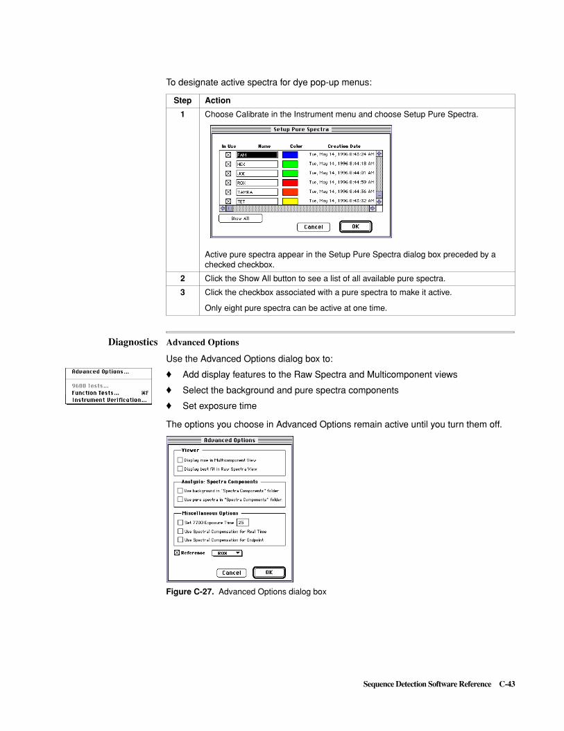
Sequence Detection Software Reference C-43
Diagnostics Advanced Options
Use the Advanced Options dialog box to:
� Add display features to the Raw Spectra and Multicomponent views
� Select the background and pure spectra components
� Set exposure time
The options you choose in Advanced Options remain active until you turn them off.
Figure C-27. Advanced Options dialog box
To designate active spectra for dye pop-up menus:
Step Action
1 Choose Calibrate in the Instrument menu and choose Setup Pure Spectra.
Active pure spectra appear in the Setup Pure Spectra dialog box preceded by a checked checkbox.
2 Click the Show All button to see a list of all available pure spectra.
3 Click the checkbox associated with a pure spectra to make it active.
Only eight pure spectra can be active at one time.

C-44 Sequence Detection Software Reference
The checkbox options available from this dialog box are listed and described in the following table.
Item How to Use/Description
Display mse (MSE) and best fit checkboxes
The MSE (mean squared error) in the Multicomponent view is a factor tied to the multicomponenting algorithm (see page C-54). When the appropriate pure dye spectra and background components are associated with the plate document, the MSE is less than 200 and remains flat as PCR progresses.
The best Fit for the Raw Spectra view is a representation of the appropriate pure spectra components for the selected well. When the appropriate pure dye spectra components are associated with the sample in the well, the Fit closely resembles the Raw Spectra curve.
Use background and pure spectra Components checkboxes (optionally Reanalyze data)
When the Sequence Detection application saves a plate document that contains collected fluorescence data, it also saves the Background and Pure Spectra components used during data analysis. Whenever you re-open that plate and re-analyze the data, the Sequence Detection application automatically re-uses the original, saved Background and Pure Spectra components.
You may recalibrate the Pure Spectra and Background components and then re-analyze data on a saved plate document, using the new components, as described below:
To view MSE and best Fit:
Step Action
1 Choose Diagnostics in the Instrument menu, then choose Advanced Options.
2 In the section titled Viewer, click the appropriate checkboxes to select MSE or Fit.
3 Click OK to close the dialog box. When only one well is selected, the MSE appears in the Multicomponent view and the Fit appears in the Raw Spectra view.
To re-analyze data with new spectra components:
Step Action
1 Open the plate document you wish to re-analyze.
2 Choose Diagnostics in the Instrument menu, then choose Advanced Options.
3 Click the appropriate checkboxes to select the Pure Spectra or Background components currently installed on the computer.
4 Click OK to close the dialog box.
5 Choose Analyze in the Analysis menu to re-analyze the data.
6 To save the re-analyzed data with a new plate document name, choose the Save As command.

Sequence Detection Software Reference C-45
Spectral Compensation. The two remaining options, respectively, enable spectral compensation for Real Time data or for Endpoint data (Plate Read type runs).
Functions Test The Functions Test dialog box, shown in Figure C-28, is one of two SDS Application displays which can be used by customers to verify instrument operation or troubleshoot simple problems.
Figure C-28. Functions Tests Dialog Box
The various functional areas of the dialog box are described in the first table on the next page. The second table provides a procedure for scanning a fluorescent sample.
Set 7700 Exposure Time
By default, the laser beam is directed into each well on the 96-well plate for 25 milliseconds to excite the fluorescent dyes. You may increase this exposure time to increase the ratio of fluorescent signal to noise. The acceptable range of exposure time is 5—255 milliseconds.
The fiber optic cables transport both the laser beam into the wells to excite the dyes and the resulting emission out of the wells toward the CCD camera. When you increase the exposure time, you also increase the amount of time between emission collections. Therefore, when you increase the exposure time, fewer data points are collected in a given extension time. To increase the number of data collected during extension, you must increase the extension time.
IMPORTANT Increasing exposure time above 25 milliseconds may result in a signal that exceeds the measuring capabilities of the optical system.
Use Spectral Compensation for Real Time/Endpoint
The two remaining options, respectively, enable spectral compensation for Real Time data or for Endpoint data (Plate Read type runs).
Item How to Use/Description

C-46 Sequence Detection Software Reference
Description of Dialog Box
This dialog box (opened by choosing the Functions Test command from the Instrument/Diagnostics submenu) enables manual control of the following instrument hardware. The various portions of the dialog box function as described in the table below:
To scan a fluorescent sample, proceed as follows:
Laser Power This portion of the dialog box is used to turn on the instrument laser and set the laser power level.
The laser is turned on by clicking the “Run” radio button and idled by clicking the “Idle” radio button. The laser power output is set by entering a value in the “Measured” field. The current status of the laser is displayed at the bottom of the window area.
Multiplexer This portion of the dialog box is used to move the multiplexer to designated positions or return it to the Home position.
The multiplexer is moved in either of two ways to the desired position. Either enter the value of the desired position in the entry field and then click the “Move To”” radio button or, click the up or down arrow until the desired position is shown in the “Position” indicator. The multiplexer is moved to the “Home” position by clicking the “Home” button.
Shutter This portion of the dialog box is used to open and close the instrument shutter (showing the current condition of the shutter).
CCD Camera This portion of the dialog box is used to change to manual CCD (Charge Coupled Device) polling and initiate polling of the CCD.
Turn to the manual shutter control mode by clicking the “Manual” radio button. Return to the Automatic mode by clicking this radio button. The “Poll CCD” button is used to initiate a CCD Read.
CCD Read area When polling is initiated, the resulting signal is displayed in this area of the window.
Save CCD . . . this portion of the window enables saving of CCD Reads to Disk by clicking the “File” button and selecting the desired file in the dialog box which appears. The “Comment” field enables saving a comment with a read. The “Set Integration Time” button makes this setting for a CCD read.
The Functions Test dialog box can be used to check signal throughput of the system by scanning a fluorescent sample such as a TaqMan PCR tray or a fluorescent test tray.
Step Action
1 Load a fluorescent sample into a plate position.
2 Click the Run button (Laser power), enter 10 mW in the “Measured” entry field and set this value for laser power by clicking the Set button.
3 Open the shutter by clicking the Shutter button.
4 Move the Multiplexer to the position containing the fluorescent sample either by entering a position number and then clicking the “Move To” button or by repeatedly clicking the up or down arrow.
5 Click the Manual radio button and then click Poll CCD to produce a fluorescent signal for the selected sample well.
Note You may store the CCD read in a designated file if you desire.

Sequence Detection Software Reference C-47
The above test can answer the following questions in troubleshooting the instrument:
� Is laser light getting to the sample?
� Do the shutters open?
� Is the Multiplexer stopping at the correct position?
� Is the CCD operating properly?
IMPORTANT Results obtained from this test menu are dependent upon the quality and reproducibility of the fluorescent test tray and sample used during testing.
InstrumentVerification
The dialog box shown in Figure C-29 is opened using the Instrument Verification command. This window initiates testing of the instrument’s electronics, and checks the version of software and firmware being used with the system.
Figure C-29. SDS Instrument Verification Dialog Box.
To confirm a problem with your instrument, report the results shown in this window to your Applied Biosystems Service representative.

C-48 Sequence Detection Software Reference
Analysis Menu
Purpose of Menu Use the commands in the Analysis Menu to display and analyze collected data.
Figure C-30. Analysis Menus for the Two Analytical Plate Types
The Analysis menu provides different choices for the two types of analysis plates.
Note The above Analysis menus are those presented after Analysis. Before Analysis, the only choice besides “Analyze” is “Raw Spectra.”
Display Offers a choice of three data display options:
� Sample Type
� Quantity
� D Rn
Note Quantity and D Rn data options are active only after data has been analyzed).
The display options change the text that appears in the 96 wells in the Analysis view of the plate document and are described in the table below:
continued on next page
Single Reporter Allelic Discrimination
The Allelic Discrimination command is available only after Analysis.
Item Description
Sample Type Displays the sample type assigned on the Setup view.
Quantity After data has been analyzed, choose Quantity to see the calculated starting quantity appear in each well. Quantity is expressed in scientific notation. (See page C-7 for a discussion of scientific notation.)
D Rn (Delta Normalized Reporter)
Choose DRn to see the values for normalized reporter minus baseline appear in each well. Normalized reporter is the reporter signal divided by the passive reference signal. If your experiment uses more than one reporter dye, look at each corresponding dye layer on the plate document.
If you choose None as the Reference dye, the Reporter signal is not normalized. The Y (vertical) axis on the Amplification Plot of Rn or DRn vs. Cycle (see page C-52) displays fluorescence emission values, not normalized signal, when you choose None as the Reference dye.

Sequence Detection Software Reference C-49
Options This command is used to set Analysis Options. The default settings are as follows:
� All data analysis is done using the Post-PCR reading only. Deselect the “Analyze using Post Read Data Only” checkbox to subtract the Pre-PCR reading from the Post-PCR reading.
� The “Show threshold” checkbox applies only to the ABI PRISM 7700 system.
� The “Automatically compute” checkbox applies only to the ABI PRISM 7700 system.
Statistics/AlleleSettings
Both of these Analysis menu (Figure C-30 on page C-48) commands are available for Allelic Discrimination plates. Only the Statistics Settings command is available for a Single Reporter Plate read.
Statistics Settings
This command presents the following dialog box, allowing the confidence level to be set. The value shown is the default.
Figure C-31. Statistics Settings dialog box

C-50 Sequence Detection Software Reference
Allele Settings
This command presents the following dialog box, allowing the allele call designators to be reassigned. The designators shown are the defaults.
Figure C-32. Allele Settings dialog box
AllelicDiscrimination
General
The window brought up by this command is used to view Allelic Discrimination results.
This command presents a detailed look at the experimental results produced by the Allelic Discrimination assay. This viewer is only active for Allelic Discrimination plate types. After analysis, the command brings up a display like that shown below:
Figure C-33. Information displayed in the Allelic Discrimination View
Graphical Views
The main features of the Allelic Discrimination viewer are:
� A graph of the data with three views at the top of the viewer
� A table of results in 11 columns in the middle of the viewer
� A table of Allele calls for each plate position at the bottom of the viewer
Graphical display area
Graphical view selector
Allelic Discrimination data
Allelic Discrimination callsfor all wells
Allele call selector
Graphical tools
(see Legend below)

Sequence Detection Software Reference C-51
The graphics viewer has three controls:
� A graphical view selector to move between the three graphical views
� Buttons to select a graphics selection tool
� An Allele call selector to manually change the calls
Three graphical views are presented to display the results from the middle table. These views and the associated data are:
� Dye components - TET Rn, FAM Rn
� Allele components - T1m, T2m
� Normalized - T1n, T2n
Graphical Tools
The buttons at the top of the viewer allow you to perform a number of operations on the data.
When you click an individual data point(s), or lasso a group of points with a selector button, the corresponding field(s) in the bottom table are highlighted.
The following buttons allow you to move the graph and change the magnification:
The position button allows you to reposition the displayed data while preserving the magnification.
The zoom buttons are used to change the magnification of the entire graph.
There are two ways to zoom. You can choose your desired zoom button and click on the graph at the point to be centered. Or you can click and drag to create a frame for the area to be magnified.
continued on next page
Individual data point selector
Group of data points selector

C-52 Sequence Detection Software Reference
Amplification Plot When the Show Threshold checkbox is enabled in Preferences, the following version of the Amplification plot is presented automatically after Analysis for Single Reporter plates enabling you to set the threshold value for all Reporter layers.
Figure C-34. Amplification Plot Window, Semilog View
Use of the command after analysis displays analyzed data for each selected well in three different formats:
� Threshold cycle (CT) vs. well number
� Rn vs. cycle
� DRn vs. cycle
Note To display the Y-axis of the Amplification Plot graph in the linear mode, as shown in Figure C-35, double-click on the Y-axis and use the dialog box to select the linear mode:
Figure C-35. Linear Mode Graph
To view the Amplification Plot:
Step Action
1 In the Analysis view of the plate document, select one or more wells.
2 Choose View and Amplification Plot in the Analysis menu. Sample data can be presented in any of the forms shown on the next page using the Display pop-up.

Sequence Detection Software Reference C-53
Note Threshold cycle calibration data in two lower figures has been truncated. Each of the lower figures has the same Threshold Cycle Calibration box as the first.
3 Use the Display pop-up on the Amplification Plot window to look at data in each of the three plot formats.
4 Use the Dye pop-up on the Amplification Plot window to look at data associated with different reporter dyes.
To view the Amplification Plot: (continued)
Step Action
Rn vs. Cycle
CT vs. Well Number
Display pop-up
Dye pop-up
DRn vs. Cycle
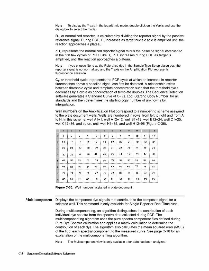
C-54 Sequence Detection Software Reference
Note To display the Y-axis in the logarithmic mode, double-click on the Y-axis and use the dialog box to select the mode.
Rn, or normalized reporter, is calculated by dividing the reporter signal by the passive reference signal. During PCR, Rn increases as target nucleic acid is amplified until the reaction approaches a plateau.
DRn represents the normalized reporter signal minus the baseline signal established in the first few cycles of PCR. Like Rn, DRn increases during PCR as target is amplified, until the reaction approaches a plateau.
Note If you choose None as the Reference dye in the Sample Type Setup dialog box, the reporter signal is not normalized and the Y axis on the Amplification Plot represents fluorescence emission.
CT, or threshold cycle, represents the PCR cycle at which an increase in reporter fluorescence above a baseline signal can first be detected. A relationship exists between threshold cycle and template concentration such that the threshold cycle decreases by 1 cycle as concentration of template doubles. The Sequence Detection software generates a Standard Curve of CT vs. Log [Starting Copy Number] for all standards and then determines the starting copy number of unknowns by interpolation.
Well numbers on the Amplification Plot correspond to a numbering scheme assigned to the plate document wells. Wells are numbered in rows, from left to right and from A to H. In this scheme, well A1=1, well A12=12, well B1=13, well B12=24, well C1=25, well C12=36, and so on, until well H1=85, and well H12=96 (Figure C-36).
Figure C-36. Well numbers assigned in plate document
Multicomponent Displays the component dye signals that contribute to the composite signal for a selected well. This command is only available for Single Reporter Real Time runs.
During multicomponenting, an algorithm distinguishes the contribution of each individual dye spectra from the spectra data collected during PCR. The multicomponenting algorithm uses the pure spectra component files defined during Pure Dye Spectra calibration and applies a matrix calculation to determine the contribution of each dye. The algorithm also calculates the mean squared error (MSE) of the fit of each spectral component to the measured curve. See page C-18 for an explanation of the multicomponenting algorithm.
Note The Multicomponent view is only available after data has been analyzed.

Sequence Detection Software Reference C-55
To open the Multicomponent view of one well:
The Y (vertical) axis of the Multicomponent View is divided into two sections. The top section of the Y axis represents emission intensity; the bottom section represents temperature. The X (horizontal) axis represents data Readings. By default, a data reading is collected approximately once every 7 seconds.
The area labeled “Component Series” displays each component in the Multicomponent View with its associated checkbox and color. If the TaqMan fluorogenic probe in an experiment is labeled with a reporter dye other than FAM, the FAM component still appears in the Multicomponent view. This is due to the presence of FAM in the passive reference.
Raw Spectra Displays reporter fluorescence signal that is not normalized for each cycle of PCR. When you click the best Fit checkbox in the Advanced Options dialog box, the Raw Spectra view also displays a line labelled Fit (page C-44). Fit represents the pure spectra component signal for the selected well and should closely resemble the Raw Spectra curve.
Typically, the fluorescence signals in the first two bins of pure spectra data are too small to be measured and are not included in the Fit calculation. As a result, the Fit line does not start at the Y axis.
Step Action
1 In the Analysis view of the plate document, select a well.
2 Choose View and Multicomponent in the Analysis menu.
To view the Pure Spectra and Fit for any well:
Step Action
1 After data collection is complete, select a well in the Analysis view of the plate document.
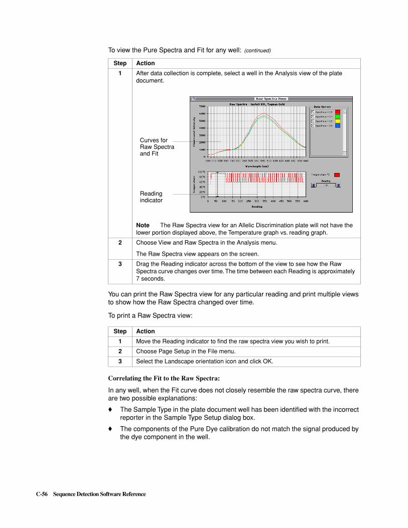
C-56 Sequence Detection Software Reference
You can print the Raw Spectra view for any particular reading and print multiple views to show how the Raw Spectra changed over time.
To print a Raw Spectra view:
Correlating the Fit to the Raw Spectra:
In any well, when the Fit curve does not closely resemble the raw spectra curve, there are two possible explanations:
� The Sample Type in the plate document well has been identified with the incorrect reporter in the Sample Type Setup dialog box.
� The components of the Pure Dye calibration do not match the signal produced by the dye component in the well.
1 After data collection is complete, select a well in the Analysis view of the plate document.
Note The Raw Spectra view for an Allelic Discrimination plate will not have the lower portion displayed above, the Temperature graph vs. reading graph.
2 Choose View and Raw Spectra in the Analysis menu.
The Raw Spectra view appears on the screen.
3 Drag the Reading indicator across the bottom of the view to see how the Raw Spectra curve changes over time. The time between each Reading is approximately 7 seconds.
Step Action
1 Move the Reading indicator to find the raw spectra view you wish to print.
2 Choose Page Setup in the File menu.
3 Select the Landscape orientation icon and click OK.
To view the Pure Spectra and Fit for any well: (continued)
Step Action
Curves for Raw Spectra and Fit
Reading indicator
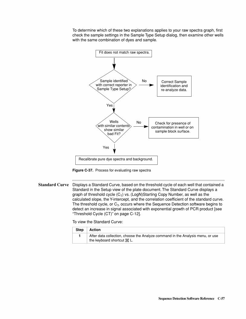
Sequence Detection Software Reference C-57
To determine which of these two explanations applies to your raw spectra graph, first check the sample settings in the Sample Type Setup dialog, then examine other wells with the same combination of dyes and sample.
Figure C-37. Process for evaluating raw spectra
Standard Curve Displays a Standard Curve, based on the threshold cycle of each well that contained a Standard in the Setup view of the plate document. The Standard Curve displays a graph of threshold cycle (CT) vs. (LogN)Starting Copy Number, as well as the calculated slope, the Y-intercept, and the correlation coefficient of the standard curve. The threshold cycle, or CT, occurs where the Sequence Detection software begins to detect an increase in signal associated with exponential growth of PCR product [see “Threshold Cycle (CT)” on page C-12].
Fit does not match raw spectra.
Sample identified with correct reporter in Sample Type Setup?
No
Yes
Correct Sample identification and re-analyze data.
Wells with similar contents
show similar bad Fit?
No
Yes
Recalibrate pure dye spectra and background.
Check for presence of contamination in well or on
sample block surface.
To view the Standard Curve:
Step Action
1 After data collection, choose the Analyze command in the Analysis menu, or use the keyboard shortcut c L.

C-58 Sequence Detection Software Reference
While you cannot select which wells to view, you may change the standard curve by going back to the Setup view of the plate document and removing the Standard sample type from one or more wells and then re-analyzing data.
You may print the Standard Curve when it is in the active window on your screen.
2 Select any one well on the Analysis view of the plate document and choose the Standard Curve command. The Standard Curve appears on the screen).
To re-calculate a Standard Curve:
Step Action
1 In the Analysis view, select all wells that contain the Standard sample type.
2 Choose View and Amplification Plot in the Analysis menu.
3 Review the Rn and CT of each well to determine which wells you want to exclude from the standard curve calculations.
4 Toggle the plate document view to the Setup view.
5 Select the wells you want to exclude from the standard curve calculation.
6 In the Sample Type pop-up menu, choose Not In Use.
7 Return to the Analysis view of the plate document.
8 Choose Analyze in the Analysis menu.
9 Select any one well on the plate document. Choose View and Standard Curve in the Analysis menu.
The re-calculated Standard Curve appears on the monitor screen.
To print the Standard Curve:
Step Action
1 Click the Standard Curve view to make it the active window.
2 Choose Page Setup in the File menu.
3 Select the Landscape orientation icon and click OK.
4 Choose Print in the File menu.
5 Click Print.
To view the Standard Curve: (continued)
Step Action

Sequence Detection Software Reference C-59
Graph Features
General The graphs in the Raw Spectra, Multicomponent and Amplification Plot views share common features that you can use to change the appearance of the data.
Changing SpectraDisplayed
In the Pure Spectra, Raw Spectra view and Amplification Plot, you can view spectra data from multiple wells simultaneously, while the Multicomponent view displays multiple component spectra for one well. You can use the checkboxes associated with each spectrum to remove and then bring back each line. You can also change the colors associated with each spectrum.
Figure C-38. Raw Spectra from Multiple Wells
Checkbox Toggles
Each graph has a list of displayed spectra, each with a checkbox and a colored square.
The checkboxes in these areas act like a toggle switch. When a checkbox is selected, the associated spectrum appears; when a checkbox is blank, the spectrum goes away.
To remove spectra in a graphic display:
� Click the checkbox adjacent to the list entry.
List with checkboxes
View List name List entries
Pure Spectra Sample (Well) Dyes by well number
Raw Spectra Data Series Wells by number
Multicomponent Component Series Component spectra
Amplification Plot Samples Wells by number

C-60 Sequence Detection Software Reference
Colors Assigned to Spectra
The Sequence Detection application automatically assigns colors to spectra when it displays a graph. You can override these color assignments.
To change the color associated with a spectrum:
Changing GraphDisplay Features
On all the graphs, you can change: the scale of the Y and X axes; the border, area, and grid of the graph area; and the graph type.
To change the scale on an axis:
Step Action
1 Double-click the color box associated with a spectrum.
A dialog box displays a color wheel.
2 Choose a new color for the spectrum and click OK.
Step Action
1 Double-click the numbers on the axis.
A box appears around the numbers on the axis as the Format Axis dialog box appears.
2 Enter values in the fields labeled “Maximum value, ” and “Minimum value” to change the scale of the selected axis.
3 Click OK to close the dialog box.
Scale options

Sequence Detection Software Reference C-61
To change the graph area display:
To change the graph type:
Step Action
1 Double-click inside the border of the graph.
The Format Plot Area dialog box appears.
2 Select features in the Border, Area and Grid portions of this dialog box and the click OK to see how the graph display changes.
Step Action
1 Double-click inside the border of the graph to open the Format Plot Area dialog box.
2 Select a Graph Type option and click OK to see how the graph display changes.

C-62 Sequence Detection Software Reference
Windows Menu
General Use these commands to switch between the Setup and Analysis views and open the Experiment Report and the Event Log.
Experiment Report Displays a summary of the contents of the plate document including:
� File Name, User Name, Date of experiment, Sequence Detector model number, Plate Type, PCR sample volume, and Comments
� The method described in the Thermal Cycler Conditions box
� Standard Curve statistics
� Contents of each well, calculated threshold cycle, quantity, and replicate mean and standard deviation
Analysis results are available in the Experiment Report only after data is analyzed. When you open a saved plate document, you must re-analyze the data to see analysis results on the Experiment Report.
Note Raw data is saved when a plate document is closed, but it must be re-analyzed when the plate is re-opened. Analyzed data is not saved when the plate document is closed.
You cannot edit the values displayed in the Experiment Report. You can change the calculated results by first changing the Setup, either the Sample Type assigned to one or more wells or the spectra components used during data analysis, and then re-analyzing the data.
To change the values on an Experiment Report:
Step Action
1 Click the Show Setup button to see the Setup view of the plate document.
2 Select one or more wells in the Setup view.
3 Choose Not In Use in the Sample Type pop-up menu.
The selected wells are no longer associated with a sample type. The data associated with that well in that dye layer will not be included in the data analysis.
4 Click the Show Analysis button to go to the Analysis view.
5 Choose Analyze in the Analysis menu.
The wells selected in step 2 are no longer associated to analyzed data.

Sequence Detection Software Reference C-63
To view an Experiment Report:
� Choose the Experiment Report command in the Windows menu.
Figure C-39. Experimental Report window
Event Log Lists error messages or events that occur during PCR or data analysis.
Figure C-40. Event Log window
To view the Event Log:
� Choose Event Log in the Windows menu.
Whenever certain errors occur during PCR or data analysis, the Event Log automatically opens on the monitor screen. The Event Log displays the time the error occurred and briefly describes the error.
Setup view information
Thermal Cycler Conditions
Standard Curve statistics
Results of data analysis

C-64 Sequence Detection Software Reference
Table C-6 Error Messages Displayed in Event Log
Error Message Significance
Background spectra not found. Multicomponenting does not include background component. Analysis is probably wrong.
No standard curve generated--all standards have the same quantity.
In Setup view, all STND sample types have same or no quantity assigned. Quantity of UNKN sample types cannot be determined.
Standard curve generated, no unknowns to interpolate.
No UNKN sample types on Setup view.
SVDCMP: No convergence in 30 iterations.
Two of pure spectra components have same spectra or one spectra component is zero.
Well nn: Background spectra not found Multicomponenting for one well does not include background component. Analysis is probably wrong.
Well nn: Invalid quantity specified for standard.
One or more of wells with STND sample type has no quantity assigned to it. Those wells excluded from Standard Curve calculation.
Well nn: Invalid threshold cycle for standard.
The calculated CT for a well with STND sample type is either less than 1 or greater than the number of cycle repetitions. That well is excluded from the Standard Curve calculation.
Well nn: Invalid threshold cycle for unknown.
The calculated CT for a well with UNKN sample type is either less than 1 or greater than the number of cycle repetitions. The quantity for the UNKN sample cannot be determined.
Unknowns specified with no standards.
In Setup view, no wells contain STND sample types. Standard Curve cannot be generated and quantity of UNKN sample types cannot be determined.

Theory of Operation D-1
Theory of Operation D
Overview
Introduction This appendix provides an overview of the TaqMan® PCR chemistry design, optimization, and analysis.
In This Appendix This appendix has the following content:
Topic See page
Fluorescence Detection on the ABI PRISM 7700 Instrument D-3
General D-3
Fluorescence Signals Change During PCR D-3
Normalization of Reporter Signal D-3
Initial Template Concentration and Cycle Number D-4
Determination of Initial Concentration of Unknowns D-5
Kinetic Analysis/Quantitative PCR D-6
Fluorescence vs. Amplified Product D-6
TaqMan Probe Design and Function D-7
General D-7
Probe Design D-7
TaqMan Probe Behavior During PCR D-7
Factors That Influence Performance D-9
General D-9
Quenching D-9
Probe and Primer Hybridization Efficiency D-10
Efficiency of Cleavage D-10
Designing Probes D-11
Probe Length D-11
Reaction Conditions D-11
Use of Estimated Melting Temperatures D-11
Probes Available from Applied Biosystems D-12
Allelic Discrimination D-13
Cleavage of Multiple Probes D-13
Polymorphic nucleotide D-13
Comparison of Anneal/Extend Temperatures D-13
D

D-2 Theory of Operation
Single Reporter D-13
The Single Reporter Experiment D-13
Single Reporter with Internal Positive Controls D-13
Multicomponenting D-15
Definition D-15
Example D-15
Guidelines to Assay Development on the Sequence Detector D-17
Nine-step Program D-17
Identify Target Sequence D-17
Design Probes and Primers D-17
Order Reagents D-18
Quantitate Probes and Primers D-19
Prepare Master Mix D-19
Run First Test D-20
Optimize Primer Concentrations D-20
Optimize Probe Concentrations D-21
Run Your Custom Assay D-21
References D-22
Topic See page

Theory of Operation D-3
Fluorescence Detection on the ABI PRISM 7700 Instrument
General During PCR, the multiplexer directs an argon ion laser through fiber optic cables that terminate above each position on the 96-well plate. The light passes through the MicroAmp Optical Caps and, for a default time of 25 milliseconds, the laser excites the fluorescent dyes present in each well. The fiber optic cables then collect the fluorescence emission between 500 nm and 660 nm from each of the wells, with a complete collection of data from all wells approximately once every 7 seconds.
A system of lenses, filters, and a dichroic mirror focus the fluorescence emission into a spectrograph. The spectrograph separates the light (based on wavelength) into a predictably spaced pattern across a charge-coupled device (CCD) camera. The Sequence Detection application collects the fluorescent signals from the CCD camera and applies data analysis algorithms.
Figure D-1. Graphic representation of fluorescence detection system
Fluorescence SignalsChange During PCR
Figure D-2 shows how the fluorescence signals of reporter, quencher, and passive reference dyes change during PCR for a system with one fluorogenic probe and one target template.
Figure D-2. Reporter, quencher, and passive reference signal changes during PCR
Normalization ofReporter Signal
While Figure D-2 illustrates absolute change in emission intensity, the Sequence Detection application displays cycle-by-cycle changes in normalized reporter signal for the 7700 instrument. Reporter signal is normalized by dividing by the fluorescence signal of the passive reference.
96-well plateFiber optic cables
Multiplexer
Lens
Dichroic mirror
Laser source
CCD Camera
Lens
Spectrograph
Reporter
Quencher
Passive Reference
Cycle

D-4 Theory of Operation
Initial TemplateConcentration and
Cycle Number
General
At any given cycle within the exponential phase of PCR, the amount of product is proportional to the initial number of template copies. When one template is diluted several times, as with the Beta-actin target in the TaqMan DNA Template Reagent Kit (P/N 401970), the ratio of template concentration to detectable signal is preserved within the exponential and linear phases for all dilutions (Figure D-3). This relationship appears to change as rate of amplification approaches a plateau.
Figure D-3. The effect of initial concentration on Rn vs. cycle number
Threshold Cycle (CT)
On the graph of Rn vs. Cycle Number (Figure D-3), the threshold cycle occurs where the Sequence Detection application begins to detect the increase in signal associated with exponential growth of PCR product.
To determine CT, the Sequence Detection application collects data from the first few PCR cycles and calculates the average Rn and the standard deviation of the Rn of these cycles. In most PCR systems, the first 15 cycles represent the baseline. Next, the algorithm multiplies the standard deviation of the background Rn by a default factor of 10 to define a threshold. Finally, the algorithm searches the data for a point that exceeds the baseline by the value of the threshold. The cycle at which this point occurs is defined as CT.
CT represents a detection threshold for the Sequence Detector. CT is dependent on the starting template copy number, and the efficiency of both the DNA amplification the PCR system and the cleavage of the TaqMan fluorogenic probe. When the starting concentration of a template remains constant as the concentration of other PCR components varies, the most efficient PCR system has the lowest CT.
continued on next page
Cycle Number
Rn
Ct

Theory of Operation D-5
Determination ofInitial
Concentration ofUnknowns
Given a range of five known concentrations of the same template, we can determine the CT of each known. We then plot the CT vs. (LogN) initial concentration (Figure D-4) to produce a standard curve.
Figure D-4. CT vs. (LogN) initial concentration of five knowns
As Figure D-4 demonstrates, given the CT of any unknown, we can interpolate its initial concentration from a standard curve when the initial concentration of the knowns bracket the concentration of the unknown.
continued on next page
(LogN) initial concentration
CT
Unknown
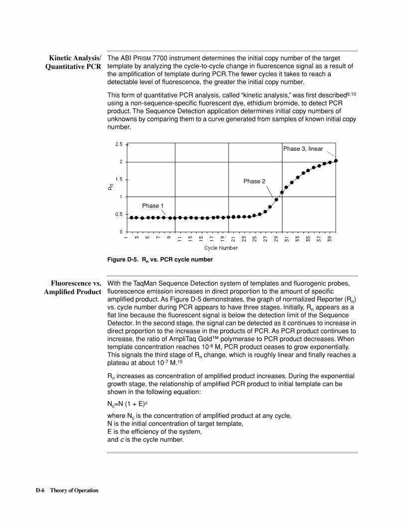
D-6 Theory of Operation
Kinetic Analysis/Quantitative PCR
The ABI PRISM 7700 instrument determines the initial copy number of the target template by analyzing the cycle-to-cycle change in fluorescence signal as a result of the amplification of template during PCR.The fewer cycles it takes to reach a detectable level of fluorescence, the greater the initial copy number.
This form of quantitative PCR analysis, called “kinetic analysis,” was first described9,10 using a non-sequence-specific fluorescent dye, ethidium bromide, to detect PCR product. The Sequence Detection application determines initial copy numbers of unknowns by comparing them to a curve generated from samples of known initial copy number.
Figure D-5. Rn vs. PCR cycle number
Fluorescence vs.Amplified Product
With the TaqMan Sequence Detection system of templates and fluorogenic probes, fluorescence emission increases in direct proportion to the amount of specific amplified product. As Figure D-5 demonstrates, the graph of normalized Reporter (Rn) vs. cycle number during PCR appears to have three stages. Initially, Rn appears as a flat line because the fluorescent signal is below the detection limit of the Sequence Detector. In the second stage, the signal can be detected as it continues to increase in direct proportion to the increase in the products of PCR. As PCR product continues to increase, the ratio of AmpliTaq Gold™ polymerase to PCR product decreases. When template concentration reaches 10-8 M, PCR product ceases to grow exponentially. This signals the third stage of Rn change, which is roughly linear and finally reaches a plateau at about 10-7 M.15
Rn increases as concentration of amplified product increases. During the exponential growth stage, the relationship of amplified PCR product to initial template can be shown in the following equation:
Nc=N (1 + E)c
where Nc is the concentration of amplified product at any cycle,N is the initial concentration of target template,E is the efficiency of the system, and c is the cycle number.
Phase 1
Phase 2
Phase 3, linear

Theory of Operation D-7
TaqMan Probe Design and Function
General The unique design of TaqMan® probes, combined with the 5´ - 3´ nuclease activity of AmpliTaq Gold™ polymerase1, 2, 3,4 (Figure D-6), allows direct detection of PCR product by the release of a fluorescent reporter during the PCR on the ABI PRISM®
7700 Sequence Detector.2,,5,6
Figure D-6. Stepwise representation of Taq DNA
Note The figure represents the fork-like, structure-dependent, 5´ to 3´ polymerization- associated nuclease activity of Taq DNA polymerase during one extension phase of PCR.3
Probe Design The TaqMan probe consists of an oligonucleotide with a 5´-reporter dye and a downstream, 3´-quencher dye. The fluorescent reporter dye, such as FAM (6-carboxy-fluorescein), is covalently linked to the 5´ end of the oligonucleotide. TET (tetrachloro-6-carboxy-fluorescein), JOE (2,7-dimethoxy-4,5-dichloro-6-carboxy- fluorescein), and HEX (hexachloro-6-carboxy-fluorescein) may also be used as reporter dyes. Each of the reporters is quenched by TAMRA (6-carboxy-tetramethyl- rhodamine), typically located at the 3´ end.
TaqMan ProbeBehavior During
PCR
When the probe is intact, the proximity of the reporter dye to the quencher dye results in suppression of the reporter fluorescence, primarily by Förster-type energy transfer 7,8. During PCR, forward and reverse primers hybridize to a specific sequence of the target DNA. The TaqMan probe hybridizes to a target sequence within the PCR product. The AmpliTaq Gold enzyme cleaves the TaqMan probe with its 5´–3´

D-8 Theory of Operation
nuclease activity. The reporter dye and quencher dye are separated upon cleavage, resulting in increased fluorescence of the reporter (Figure D-6 on page D-7). The 3´ end of the TaqMan probe is blocked to prevent extension of the probe during PCR.
This process occurs in every cycle and does not interfere with the exponential accumulation of product. The separation of the reporter dyes from the quencher dye results in increase in fluorescence for the reporter. The increase in fluorescence is measured, and is a direct consequence of target amplification during PCR.
Both primer and probe must hybridize to the target for amplification and cleavage to occur. The fluorescence signal is generated only if the target sequence for the probe is amplified during PCR. Because of these requirements, non-specific amplification is not detected. For information on release of a fluorescent reporter during the PCR, refer to Lee et al., 1993, and Livak et al., 1995.

Theory of Operation D-9
Factors That Influence Performance
General Three main factors determine the performance of a doubly labeled fluorescent probe in this 5' nuclease assay: quenching of intact probe; hybridization efficiency; and efficiency of cleavage by AmpliTaq Gold polymerase. For other factors which influence performance, see “Guidelines to Assay Development on the Sequence Detector” on page D-17.
Quenching Dye Placement
Fluorescence quenching depends on the spatial proximity of the reporter and quencher dyes. In fact, Förster-type energy transfer efficiency varies with the inverse sixth power of the distance between fluorophores. It was originally thought that the quencher dye must be close to the 5´ end in order to achieve adequate quenching.5 Surprisingly, the quencher dye, TAMRA, can be attached to virtually any nucleotide in a probe and still quench the fluorescence emission of a reporter dye attached to the 5´ end.11 The flexibility of a single-stranded oligonucleotide apparently allows the probe to adopt conformations where the reporter and quencher dyes are close enough to achieve energy transfer.
Avoid G at the 5´-end Position
Factors other than dye placement can effect the degree of quenching in a fluorogenic probe. We have found that a G next to the reporter dye causes some quenching, which persists even after cleavage of the fluorogenic probe. Consequently, it is best to avoid G at the 5´-end position of a fluorogenic probe.
Other Structures to Avoid
Probes with a reporter dye on the 5´ end and TAMRA on the 3´ end exhibit sufficient quenching for the fluorogenic 5´ nuclease assay. With the TAMRA at the 3´ end, quenching appears to be dependent on the flexibility of the single-stranded probe. Any structure that interferes with this flexibility could potentially reduce the degree of quenching observed in the intact probe. Probe structures to be avoided include hairpins, self-complementarity, complementarity to either the reverse or the forward PCR primer, and four or more of a single base in a row, especially Gs.
Effect of Probe Purity
Finally, the purity of the probe can have a marked effect on the observed quenching. Any molecule that has a reporter dye but no quencher dye can be a source of contamination. The presence of unquenched reporter raises the initial intensity of the reporter fluorescence, making it difficult to discern the change in reporter fluorescence that is due to probe cleavage. For this reason, the reporter dye is attached to the 5´ end using a phosphoramidite, so that any failure (incomplete)sequences generated during the oligonucleotide synthesis are not labeled with the reporter dye.
continued on next page

D-10 Theory of Operation
Probe and PrimerHybridization
Efficiency
General
Cleavage of a fluorogenic probe requires hybridization to the target sequence. All general rules for the design of hybridization probes also apply to fluorogenic probes. Such general advice includes: avoid secondary structure in probe or target site; and avoid long runs of a single nucleotide.
Avoid Probe Hybridizing with PCR Primers
In addition, the probe should not hybridize with either PCR primer. Such hybridization lowers the effective concentration of both probe and primer, reducing PCR hybridization efficiency. Probe-primer hybrids can also be a source of ‘primer-dimer’ contamination, formed during the amplification reaction.
Primer and Probe Hybrids
Both the PCR primers and the fluorogenic probe need to hybridize to the template strands during the annealing step of the PCR amplification reaction. Primer-template hybrids are stabilized when the AmpliTaq Gold enzyme extends the primer in the polymerization reaction. The fluorogenic probe is not extended, so its hybridization is not stabilized. Thus, it follows that the probe-template hybrid must be more stable (have higher Tm) than the primer-template hybrids. Also, the Tm of the probe should be higher than the actual annealing temperature used in the 5´ nuclease assay. Please refer to “Guidelines to Assay Development on the Sequence Detector” on page D-17 for further advice on primer/probe selection.
AmpErase UNG
The Tms of all the oligonucleotides need to be greater than 55 °C, due to the presence of AmpErase® UNG (uracil-N-glycosylase). UNG has significant activity below 55 °C, can degrade amplicons and thereby introduce more variability into the 5´ nuclease assay.
Efficiency ofCleavage
Although the effect on quenching may be modest, the placement of the quencher dye can have a major impact on the efficiency of cleavage by the AmpliTaq Gold polymerase. To observe an increase in reporter fluorescence intensity in the fluorogenic 5´ nuclease assay, the probe must be cleaved between the reporter and quencher dyes. When dyes are placed on opposite ends of the probe, any cleavage of the probe is detected. When the quencher dye is placed on an internal nucleotide, only cleavages that occur between the reporter and quencher dyes are detected. Therefore, synthesizing an oligonucleotide with a reporter dye on the 5´ end and TAMRA attached to the 3´ end provides the best chance of having a probe that reliably detects PCR in the fluorogenic 5´ nuclease assay.

Theory of Operation D-11
Designing Probes
Probe Length When the length of the probe increases beyond 30 nucleotides, two problems arise. First, longer probes reduce the yield of the oligonucleotide synthesis. Second, the longer the probe, the greater the chance of forming inter- or intra-molecular structures that create purification problems, impair the hybridization and cleavage of the probe, or interfere with PCR.
Note The primary structural requirement for probes is the Tm. In order to obtain a probe with a Tm of 68-70 °C, use Primer Express software.
Probes can be designed to correspond to either strand of the PCR amplicon. When complementary probes have been tested in the 5´ nuclease assay, we have observed that one probe usually gives appreciably better performance (higher DRn values) than its complement. The critical difference appears to be the C-to-G ratio in the composition of the probe.
Although the percentage G+C content of complementary sequences is identical, in general one strand will have more Cs and the opposite strand will have more Gs. We have found that those probe sequences with the greater number of Cs usually perform better in the 5´ nuclease assay.
Reaction Conditions The fact that a fluorogenic probe is not stabilized by being extended during PCR has consequences for the extension step used in amplification. As previously discussed, successful 5´ nuclease assay results require the following four events:
� primers hybridize and are extended
� probe hybridizes
� probe is cleaved, which increases fluorescence signal, and
� primer extension is completed
Since a fluorogenic probe must be hybridized for cleavage to occur, extension must be carried out at a temperature that ensures probe binding.
Note See “Guidelines to Assay Development on the Sequence Detector” on page D-17 for specific reaction conditions.
A two-temperature PCR protocol using a combined annealing/extension temperature below the Tm of the probe should increase the hybridization and cleavage efficiency of the fluorogenic probes. We have found that on the ABI PRISM 7700 Sequence Detection System, a combined anneal-extension step of 1 minute at 55 °C or higher has been sufficient for amplicons under 1 Kb.
Higher concentrations of MgCl2 (3.5–9 mM) stabilize probe binding and thus promote the use of higher temperatures during the combined anneal/extension step. Higher temperatures are desirable so that the extension rate of the AmpliTaq Gold enzyme is as high as possible.
Use of EstimatedMelting
Temperatures
The only way to know the Tm of an oligonucleotide for sure is to measure it experimentally. To design a probe, though, estimated Tms must be used. Although it is not completely accurate, the nearest neighbor method13 is the best algorithm generally available for estimating Tms of oligonucleotides.

D-12 Theory of Operation
In designing a probe for a PCR system that is already optimized, the estimated Tm of the probe should be at least 5 °C above the annealing temperature. For cases where probe and primers are being designed at the same time, we suggest that the estimated Tm of the probe be at least 5 °C higher than the matched Tms of the PCR primers.
Note Primer Express™ software is recommended for choosing TaqMan primers and probes with accurate Tm prediction. A single user copy of the software is available under P/N 402809.
Probes Availablefrom Applied
Biosystems
The three types of TaqMan fluorogenic probes listed in Table D-1 are available from Applied Biosystems. Custom probes ordered by the three Part Numbers are identical except for quantity and are HPLC-purified to minimize the amount of unquenched reporter present and give very reproducible results.
* Part numbers listed are for US only. Contact your Regional Sales Office for local Part numbers and prices (see “To Contact Technical Support by Telephone or Fax” on page 1-4 for a list of telephone and Fax numbers).
Table D-1 TaqMan Probes
Part No. * TaqMan Probes
450025 TaqMan Probe. HPLC purified. 5,000-6,000 pmol.5´ Fluorescent label: HEX, 6-FAM or TET. 3´-label: TAMRA. Labels + HPLC Purification (~ 500 reactions)
450024 TaqMan Probe. HPLC purified. 15,000-25,000 pmol.5´ Fluorescent label: HEX, 6-FAM or TET. 3´-label: TAMRA. Labels + HPLC Purification (~ 2,500 reactions)
450003 TaqMan Probe. HPLC purified. 50,000-100,000 pmol.5´ Fluorescent label: HEX, 6-FAM or TET. 3´-label: TAMRA. Labels + HPLC Purification (~ 10,000 reactions)

Theory of Operation D-13
Allelic Discrimination
Cleavage of MultipleProbes
By using different reporter dyes, cleavage of multiple probes can be detected in a single PCR. One application of this multi-probe capability is to use allele-specific probes to distinguish genetic polymorphisms.5,14 Probes that differ by as little as a single nucleotide will exhibit allele-specific cleavage. This is true even for probes with a reporter on the 5' end and TAMRA on the 3´ end.14
Polymorphicnucleotide
In designing allele-specific probes, the polymorphic nucleotide should be positioned approximately in the center of the probe because a mismatch in this position is usually the most disruptive to probe-template hybrid stability. If the polymorphism changes the G+C content (for example, a C-to-T change), the probe should be lengthened one or two nucleotides in order to compensate for Tm differences. The other elements of fluorogenic probe design still apply.
Comparison ofAnneal/ExtendTemperatures
In using the 5´ nuclease assay to distinguish alleles, it is usually necessary to compare different anneal/extend temperatures. Lower temperatures produce higher DRn values, but there may be little discrimination between alleles. Increasing the anneal/extend temperature improves the allele-specific response of the probes, but decreases overall signal. At higher temperatures, some of the signal loss can be regained by increasing the concentration of the PCR primers.
The optimum anneal/extend temperature is empirically determined to achieve the best compromise between allele discrimination and signal level.
Single Reporter
The Single ReporterExperiment
A Single Reporter experiment is designed to report the presence or absence of a specific nucleic acid sequence in a test sample. This assay only requires one TaqMan probe for detection.
Single Reporter withInternal Positive
Controls
Purpose of Internal Positive Controls
By using probes labeled with different reporters, a positive control for the PCR chemistry can be included in any amplification reaction. This Internal Positive Control (IPC) ensures that a failed PCR is not mistaken for a negative test result.
Considerations in Using an IPC
The IPC consists of a PCR template (DNA or RNA) that is spiked into the amplification reaction at known concentration. Also included in the reaction are primers and probe for detecting amplification of the IPC. The IPC probe is labeled with a different reporter than the probe used for detection of target amplification. Generally, the target probe is labeled with FAM and the IPC probe is labeled with TET or JOE.
Interpretation of Results
A positive result with the target probe indicates the target is present in the sample and there is no need to refer to the IPC amplification. On the other hand, a negative result
D-14 Theory of Operation
with the target probe could mean that the sample contains no target or that, for some reason, PCR failed in that well. Referring to the results with the IPC probe can distinguish between these two possibilities. A positive signal with the IPC probe shows that PCR amplification can occur in that well and, thus, the lack of target signal means the sample is a true negative. If amplification of the IPC is not detected, then PCR was inhibited in that tube and it is not possible to determine whether target is present in the sample or not.
Amount of IPC
The amount of IPC spiked into a reaction depends upon the detection limit desired for the target. The goal is that amplification of the IPC should not interfere with amplification of the target. For example, if a test were designed to detect 100 or more copies of target, then the copy number of IPC would generally be set at 100 or less. In this way, amplification of the IPC will not consume enough reagents to prevent detection of target amplification. Also, the IPC reaction can be optimized to determine the minimum concentrations of primers required for robust amplification.
Using the minimum concentrations reduces the likelihood of interference with the target amplification. Reconstruction experiments should be performed to validate that inclusion of the IPC does not affect target detection.
Note If attempting single copy target detection, the level of IPC would not be set at one copy per reaction because of the consequences of Poisson statistics. In attempting to pipet 1-copy aliquots, sampling probability indicates that some samples will have more than one copy and some fraction will actually have no copies. Thus, the minimum level of IPC should be about 10 copies per reaction in order to ensure that all reactions have enough copies for robust detection. Depending on the relative efficiencies of target and IPC amplification, the inclusion of 10 IPC copies may preclude single copy detection of the target.

Theory of Operation D-15
Multicomponenting
Definition Multicomponenting is the term used for distinguishing the contribution each individual dye and background component makes to the fluorescent spectra detected by the ABI PRISM 7700 Sequence Detector.
Example Figure D-7 shows one composite spectrum that represents a fluorescent reading of one well that contains a passive reference dye and a fluorogenic probe, labeled with FAM and TAMRA. This figure shows how the overlapping component dye spectra contribute to the composite spectrum. The multicomponenting algorithm on the Sequence Detection application applies matrix calculations to determine the contributions of each component dye spectra.16
Figure D-7. Composite spectrum and three component spectra
First, during the background and pure dye spectra calibrations, each component is measured across the entire range of measurable fluorescence, from 500–660 nm. As part of the calibration process, a representative signal for each component is generated and stored on the computer by the application. During each subsequent multicomponenting calculation, the application refers back to these stored representative signals and applies an algorithm to solve for a, b, c, and d in the following equation:
where a, b, c, and d represent each component’s contribution.
The algorithm solves for a, b, c, and d to find the smallest value for mean squared error (MSE). This example calculation assumes that pure dye components exist for
Wavelength
Composite spectrum
FAM TAM
ROX
Measured spectrum a FAM( ) b TAMRA( ) c ROX( ) d Background( ) Error+ + + +=

D-16 Theory of Operation
three dyes and for the instrument background. Figure D-8 shows a typical display of the contribution of each component spectra for one well.
Figure D-8. The Sequence Detection Application’s Multicomponent View
The MSE display is an optional feature. If you want the MSE to appear in the Multicomponent view, see “Advanced Options” on page C-43.
Theory of Operation D-17
Guidelines to Assay Development on the Sequence Detector
Nine-step Program The following steps are recommended for the development of custom 5´ nuclease assays.
� Identify the target sequence.
� Design the TaqMan probes.
� Design the forward and reverse Primers.
� Order reagents.
� Quantitate the concentrations of the probes and primers.
� Prepare the Master Mix.
� Run a first iteration of the test.
� Optimize the primer concentrations.
� Optimize the probe concentrations.
Identify TargetSequence
� A target is a nucleotide sequence, two primers, and a probe.
� For allelic discrimination, each allele associated with a target will have a probe labeled with its own fluorescent reporter dye.
� The shortest amplicons work the best. Consistent results are obtained for amplicon ranges from 50–200 bp.
Design Probes andPrimers
Design Probes
Use the following guidelines:
� Keep the G-C content in the range of 30–80%.
� Avoid runs of an identical nucleotide. This is especially true for guanine, where runs of four or more Gs should be avoided.
� No G on 5´ end.
� Using Primer Express™ software, Tm should be 10 °C greater than primers.
� Select the strand that gives the probe with more Cs than Gs.
� Position the polymorphism site approximately in the center.
� Adjust probe length so that both probes have the same Tm.
Design Primers
Use the following guidelines:
� Keep the G-C content in the range 30–80%.
� Avoid runs of an identical nucleotide. This is especially true for guanine, where runs of four or more Gs should be avoided.
� Using Primer Express™ software, Tm should be 58–60 °C.
� The five nucleotides at the 3´ end should have no more than two G and/or C bases.
� Place the forward and reverse primers as close as possible to the probe without overlapping the probe.
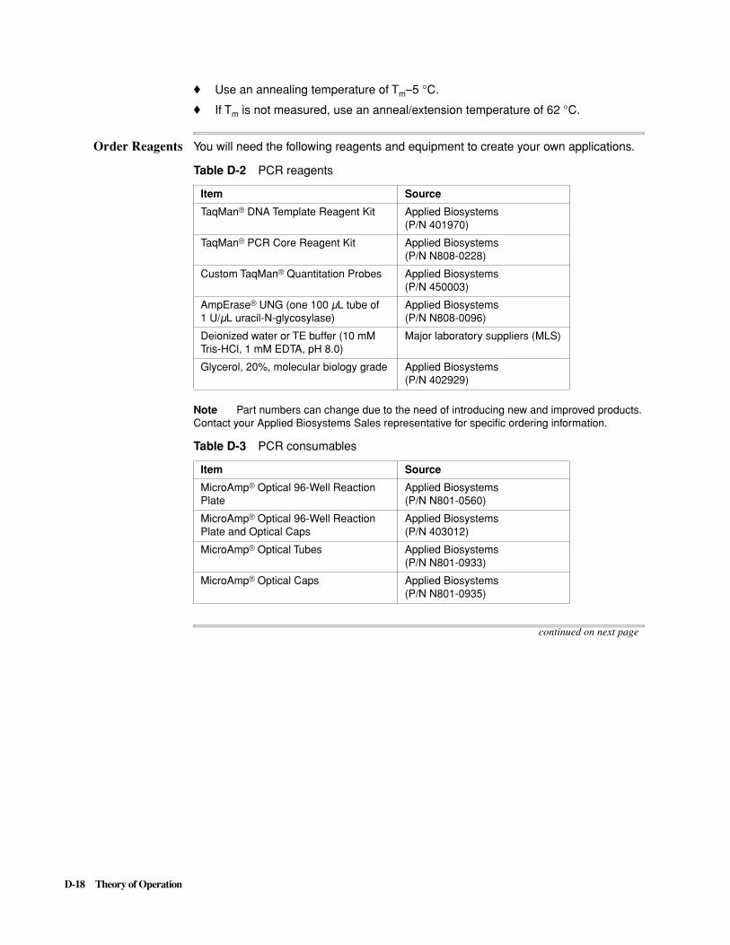
D-18 Theory of Operation
� Use an annealing temperature of Tm–5 °C.
� If Tm is not measured, use an anneal/extension temperature of 62 °C.
Order Reagents You will need the following reagents and equipment to create your own applications.
Note Part numbers can change due to the need of introducing new and improved products. Contact your Applied Biosystems Sales representative for specific ordering information.
continued on next page
Table D-2 PCR reagents
Item Source
TaqMan® DNA Template Reagent Kit Applied Biosystems (P/N 401970)
TaqMan® PCR Core Reagent Kit Applied Biosystems (P/N N808-0228)
Custom TaqMan® Quantitation Probes Applied Biosystems (P/N 450003)
AmpErase® UNG (one 100 µL tube of 1 U/µL uracil-N-glycosylase)
Applied Biosystems (P/N N808-0096)
Deionized water or TE buffer (10 mM Tris-HCl, 1 mM EDTA, pH 8.0)
Major laboratory suppliers (MLS)
Glycerol, 20%, molecular biology grade Applied Biosystems (P/N 402929)
Table D-3 PCR consumables
Item Source
MicroAmp® Optical 96-Well Reaction Plate
Applied Biosystems (P/N N801-0560)
MicroAmp® Optical 96-Well Reaction Plate and Optical Caps
Applied Biosystems (P/N 403012)
MicroAmp® Optical Tubes Applied Biosystems (P/N N801-0933)
MicroAmp® Optical Caps Applied Biosystems (P/N N801-0935)

Theory of Operation D-19
Quantitate Probesand Primers
Use a spectrophotometric method to determine the concentrations of the probes and primers received:
� Measure the absorbance at 260 nm of a 1:100 dilution of each oligonucleotide in TE buffer.
� Calculate the oligonucleotide concentration in µM using the method shown in Table D-4.
Prepare Master Mix Use 20% glycerol and the reagents in the TaqMan PCR Core Reagent Kit ((P/N N808-0228) to prepare a TaqMan Master Mix. Remove aliquots of the Master Mix and store them at 2–6 °C. Due to pipetting carry-over, 115 reactions will provide sufficient reagent for 96 wells.
Note More information on preparing and using a Master Mix are provided in Appendix A, “Guidelines to Master Mix Preparation.”
Table D-4 Example of Extinction coefficient calculation for a FAM-labeled probe
ChromophoreExtinction Coefficient Number
Extinction Coefficient Contribution
A 15,200 1 15,200
C 7,050 6 42,300
G 12,010 5 60,050
T 8,400 6 50,400
FAM 20,958 1 20,958
TAMRA 31,980 1 31,980
TET 16,255 0 –
Total – – 220,888
Absorbance (260 nm) = sum of extinction coefficient contributions ¥ cuvette pathlength ¥ concentration/100
0.13 = 220,888 M-1cm-1 ¥ 0.3 cm ¥ C/100
C = 196 µM
Table D-5 Master Mix formulation for 115 Reactions
ReagentVolume (µL) for 115 wells of 50 µL each
Final Concentration in each 50 µL reaction
20% Glycerol 1150 8%
10X TaqMan Buffer A 288 1X
25 mM MgCl2 575 5 mM
dATP 58 200 µM
dCTP 58 200 µM
dGTP 58 200 µM
dUTP 58 400 µM
AmpliTaq Gold™ DNA Polymerase (5 U/µL)
29 0.05 U/µL
AmpErase® UNG (1 U/µL) 29 0.01 U/µL
Total 2303 –
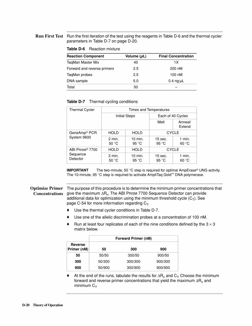
D-20 Theory of Operation
Run First Test Run the first iteration of the test using the reagents in Table D-6 and the thermal cycler parameters in Table D-7 on page D-20.
IMPORTANT The two-minute, 50 °C step is required for optimal AmpErase® UNG activity. The 10-minute, 95 °C step is required to activate AmpliTaq Gold™ DNA polymerase.
Optimize PrimerConcentrations
The purpose of this procedure is to determine the minimum primer concentrations that give the maximum DRn. The ABI PRISM 7700 Sequence Detector can provide additional data for optimization using the minimum threshold cycle (CT). See page C-54 for more information regarding CT.
� Use the thermal cycler conditions in Table D-7.
� Use one of the allelic discrimination probes at a concentration of 100 nM.
� Run at least four replicates of each of the nine conditions defined by the 3 ¥ 3 matrix below.
� At the end of the runs, tabulate the results for DRn and CT. Choose the minimum forward and reverse primer concentrations that yield the maximum DRn and minimum CT.
Table D-6 Reaction mixture
Reaction Component Volume (µL) Final Concentration
TaqMan Master Mix 40 1X
Forward and reverse primers 2.5 200 nM
TaqMan probes 2.5 100 nM
DNA sample 5.0 0.4 ng/µL
Total 50 –
Table D-7 Thermal cycling conditions
Thermal Cycler Times and Temperatures
Initial Steps Each of 40 Cycles
Melt Anneal/Extend
GeneAmp® PCR System 9600
HOLD HOLD CYCLE
2 min.50 °C
10 min.95 °C
15 sec.95 °C
1 min.60 °C
ABI PRISM® 7700 Sequence Detector
HOLD HOLD CYCLE
2 min.50 °C
10 min.95 °C
15 sec.95 °C
1 min.60 °C
Forward Primer (nM)
Reverse Primer (nM) 50 300 900
50 50/50 300/50 900/50
300 50/300 300/300 900/300
900 50/900 300/900 900/900

Theory of Operation D-21
Optimize ProbeConcentrations
The purpose of this procedure is to determine the minimum probe concentrations that give the maximum DRn and minimum CT for each probe target.
� Use the thermal cycler conditions in Table D-7 on page D-20 and the forward and reverse primer concentrations determined above.
� Run at least four replicates of each of the nine conditions defined by the 3 ¥ 3 matrix below.
� Tabulate the results for DRn and CT. Choose the minimum probe concentrations that yield the maximum DRn and minimum CT.
Note Probe optimization is specific for Allelic Discrimination assays.
Run Your CustomAssay
Run your experiment.
Probe 1 (nM)
Probe 2 (nM) 100 200 300
100 100/100 200/100 300/100
200 100/200 200/200 300/200
300 100/300 200/300 300/300

5-22
References
The references listed below are those cited by superscript numbers in the text.
5
References
1 Lawyer, F.C., Stoffel, S., Saiki R.K., Myambo, K.B., Drummond R., and Gelfand, D.H., 1989. Isolation, characterization, and expression in Escherichia coli of the DNA polymerase gene from the extreme thermophile, Thermus aquaticus. J. Biol. Chem. 264: 6427-6437.
2 Holland, P.M., Abramson, R.D., Watson, R. and Gelfand, D.H. 1991. Detection of specific polymerase chain reaction product by utilizing the 5’ to 3’ exonuclease activity of Thermus aquaticus DNA polymerase. Proc. Natl. Acad. Sci., USA 88: 7276-7280.
3 Lyamichev, V., Brow, M.A.D., Dahlberg, J.E. 1993. Structure-specific endonucleolytic cleavage of nucleic acids by eubacterial DNA polymerases. Science 260: 778-783.
4 Perkin-Elmer, 1996. AmpliTaq Gold™ Product Insert, Rev. 3.
5 Lee, L.G., Connell, C.R., and Bloch, W. 1993. Allelic discrimination by nick-translation PCR with fluorogenic probes. Nucl. Acids Res. 21: 3761-3766.
6 Gelfand, D.H., Holland, P.M., Saiki, R.K. and Watson, R.M., U.S. Patent 5 210 015, 1993; Chem Abstr. 1992.
7 Förster, V. Th., 1948, Zwischenmolekulare Energie-wanderung und Fluoreszenz. Annals of Physics (Leipzig) 2: 55-75.
8 Lakowicz, Joseph R. 1983. Chapter 10. Energy Transfer. In: Principles of Fluorescent Spectroscopy, Plenum Press, N.Y. pp, 303-339.
9 Higuchi, R., Dollinger, G., Walsh, P.S., and Griffith, R. 1992. Simultaneous amplification and detection of specific DNA sequences. BioTechnology 10:413-417.
10 Higuchi, R., Fockler, C., Dollinger, G. and Watson, R. 1993. Kinetic PCR analysis: Real-time monitoring of DNA amplification reactions. BioTechnology 11:1026-1030.
11 Livak, K., Flood, S., Marmaro, J., Giusti, W., and Deetz, K. Oligonucleotides with fluorescent dyes at opposite ends provide a quenched probe system useful for detecting PCR product and nucleic acid hybridization. PCR Methods and Applications 4: 357-362.
12 Rychlik, W., Spencer, W.J., and Rhoads, R.E. 1990. Optimization of the annealing temperature for DNA amplification in vitro. Nucl. Acids. Res. 18:6409-6412.
13 Livak, K.J., Marmaro, J., and Todd, J.A. 1995. Towards fully automated genome-wide polymorphism screening. Nature Genetics 9:341-342.
14 Bloch, W. 1991. A biochemical perspective of the polymerase chain reaction. Biochemistry 30:2735–2747.
15 Martens, H. and Naes, T., 1989. In: Multivariate Calibration, John Wiley & Sons, Chichester.

E-1 Limited Warranty Statement
Limited Warranty Statement E
Applied Biosystems (“ABD”) warrants to the customer that, for a period ending on the earlier of one year from the completion of installation or fifteen (15) month(s) from the date of shipment to the customer (the “Warranty Period”), the ABI PRISM® 7700 Sequence Detector purchased by the customer (the “Instrument”) will be free from defects in material and workmanship, and will perform in accordance with the installation specifications set forth in the system specification sheet which accompanies the Instrument or which is otherwise available from an ABD sales representative (the “Specifications”).
During the Warranty Period, if the Instrument's hardware becomes damaged or contaminated or it the Instrument otherwise fails to meet the Specifications, ABD will repair or replace the Instrument so that it meets the Specifications, at ABD's expense. However, if the thermal cycle module becomes damaged or contaminated, or if the chemical performance of the Instrument otherwise deteriorates, due to solvents and/or reagents other than those supplied or expressly recommended by ABD, ABD will return the Instrument to Specification at the customer's request and at the customer's expense. After this service is performed, warranty coverage of the Instrument will be restored thereafter for the remainder of the original Warranty Period.
This Warranty does not extend to any Instrument or part which has been (a) the subject of an accident, misuse, or neglect, (b) modified or repaired by a party other than ABD, or (c) used in a manner not in accordance with the instructions contained in the Instrument User's Manual. This Warranty does not cover the customer-installable accessories or customer-installable consumable parts for the Instrument that are listed in the Instrument User's Manual. Those items are covered by their own warranties.
ABD's obligation under this Warranty is limited to repairs or replacements that ABD deems necessary to correct those failures of the Instrument to meet the Specifications of which ABD is notified prior to expiration of the Warranty Period. All repairs and replacements under this Warranty will be performed by ABD on site at the Customer's location at ABD's expense.
No agent, employee, or representative of ABD has any authority to bind ABD to any affirmation, representation, or warranty concerning the Instrument that is not contained in ABD's printed product literature or this Warranty Statement. Any such affirmation, representation or warranty made by any agent, employee, or representative of ABD will not be binding on ABD.
ABD shall not be liable for any incidental, special, or consequential loss, damage or expense directly or indirectly arising from the purchase or use of the Instrument. ABD makes no warranty whatsoever with regard to products or parts furnished by third parties.
E

E-2 Limited Warranty Statement
This Warranty is limited to the original location of installation and is not transferable. Attempts to move or reinstall the Instrument may result in the loss of warranty coverage.
THIS WARRANTY IS THE SOLE AND EXCLUSIVE WARRANTY AS TO THE INSTRUMENT AND IS IN LIEU OF ANY OTHER EXPRESS OR IMPLIED WARRANTIES, INCLUDING, WITHOUT LIMITATION, ANY IMPLIED WARRANTY OF MERCHANT-ABILITY OR FITNESS FOR A PARTICULAR PURPOSE AND IS IN LIEU OF ANY OTHER OBLIGATION ON THE PART OF ABD.

Index-1
Index
SymbolsDRn
and data analysis 2-4and G+C content of probe D-11display C-48
•see forever hold C-26
Numerics5' nuclease assay
allelic discrimination D-13requirements D-11
7700 Sequence Detectorsample volume 3-20
96-well sample map 3-24
AA1 position
on heating block 3-29ABI PRISM 7200
importing a setup file C-21aborting
a run C-40data handling C-11
in status display C-12Acronym
Sample Type Setup C-34acronym name, changing C-34active pure spectra C-43
designating C-42adding
Data Collection icon 3-21, C-32Step, Cycle or Hold C-26
Allelic Discriminationand multiple probes D-13command, using to view
results C-50–C-51plate type C-16
Allelic Discrimination plate typesample types required C-37viewing results C-50–C-51
Amplification Plot C-52–C-54Analysis menu C-48
Allelic Discrimination command C-50–C-51
Options command C-49Analysis Options dialog box, using to
set analysis options C-49Analysis view C-10–C-13
comments C-7assigning samples to wells 3-3
Auto Incrementindicator C-30temperature 3-20, C-30time 3-20, C-30
autodecrement C-31automatic connection to
instrument 3-6, C-23
Bbackground 6-9background component C-41
advanced options C-44calibrating 3-7extract C-40in saved plate document C-17viewing C-41
Background plate type C-16best fit
in Raw Spectra view C-56viewing C-44
bin, spectral C-18Blackboard 6-9Border
on graph area C-61
Ccalculated data values, for all
wells 5-5Calibrate command C-40–C-43calibration
background component C-40spectra component C-41
CCD camera 3-26function D-3
cell culturesDNA purification B-1
channel C-18charge-coupled device, see CCDcheckbox
as toggle C-59connect to instrument 3-6Running C-23
Clear commanddeleting Steps C-28
click 5-6Clipped
exporting data C-18Collecting data C-31color
in graphs C-60sample type C-34
color, setting for sample type C-34column of wells
selecting 3-15, C-9Comm light 3-31comments
on Analysis view 3-22, C-7on Experiment Report 3-22, C-7on Setup view 3-4saving on Plate Document 3-22
componentbackground C-41, C-44pure dye C-40, C-44
Component Seriesin Multicomponent view C-55
confidence level 5-3connecting to instrument 3-6, C-23Cov. Temp. C-12cover
closing heating block 3-30opening heating block 3-32sample 3-30
creatingbackground component C-41pure spectra component C-41
CT 2-4, 2-6Cut command C-22Cycle
adding C-26counting repetitions C-13default configuration C-27definition C-25deleting C-27placement of new C-27
cycle repetitions C-13
Ddata
in saved plate document C-17Table of locations 5-4, 5-8
data analysisand extension time C-28and Run Types 2-4in Plate Read Only 2-6in Real Time run 2-6
data bin C-18data collection
and exposure time C-45and Run Type 2-4and size of files C-32eliminating C-32in Thermal Cycler
Conditions 3-19

Index-2
instrument connection C-23setting in Preferences C-23
Data Collection iconadding 3-21, C-32removing 3-21, C-32
data exportingall wells C-19selected wells C-19
decrement indicator C-30default
PCR volume C-23Step, Cycle and Hold
configurations C-27unit of measure C-23
deletingsample type in well C-62Step, Cycle, or Hold C-27
Display command C-48Sample Type C-49
displayingBackground component C-41Experiment Report 5-5heating block cover
temperature 3-5mean squared error C-44
DNA purification procedure B-1DNA purity B-12Dual Reporter
plate type C-16dye layer
definition 2-7pop-up menu 2-7, C-42viewing samples 3-16
Dye Layer pop-up menudisplaying active dyes C-34
dye pop-up C-42dye spectra
in pop-up menu C-42dyes
for Sample Types 3-3
EEdit menu C-22 editing
a method C-26 data C-62Experiment Report C-62Pure Spectra C-41Sample List
on Sample TypePalette C-33
Editing Sample Attributes command C-35
end-point analysis 2-4entry fields
Setup view C-6Event Log C-63Experiment Report C-62
and analyzed data C-62Mean C-6
Name C-23printing 5-6Replicate values C-6Std. Dev. C-6
Experiment Report, No Amp call 5-9Export command C-18exporting
All Wells C-19Selected Wells C-19
extension timerecommended C-28
extractingBackground Component C-40Background Spectra 3-8Spectra Component 3-11, C-41
FFAM D-7File menu C-16–C-21
Import command C-21Firmware 6-6Fit, best
correlation to Raw Spectra C-56floating window C-33fluorescence
detection system D-3Fluorescence Tests 6-8fluorogenic probe
design D-7 forever hold 3-32, C-26
displaying time C-12
GG+C content
of fluorogenic probes D-11GenePure Basebinder
DNA purification B-2graph
features C-59–C-61graphical tools, using on Allelic
Discrimination results C-51Grid
on graph area C-61guide, on-line 2-8guidelines
Master Mix preparation A-1–A-4PCR optimization D-17 TaqMan probe design D-7
Hheating block
closing cover 3-30cover temperature 3-5
helpon-line guide 2-8
HEX D-7Hold
adding C-26default configuration C-27
definition C-25deleting C-27forever 3-32, C-12placement of new C-27
Holdingin status display C-12
hot starts, manual 3-32hybridization
of probe and primers D-10
IIdle
in status display C-12Importing a setup file C-20importing a setup file C-21Increment indicator C-31increment indicator C-30Insert bar
determining placement C-26editing a method C-26
insertingAuto Increment C-30Auto increment C-30Step, Cycle or Hold C-26
Instrumentin Preferences C-22
Instrument menu C-40–C-43interrupting a run C-40IPC Dye Layer 5-7IPC Dye Layer, results 5-9IPC Layer setup, typical 5-7IPC+ and IPC- 5-7IPCs, how to add 5-7
JJOE D-7
Kkeyboard shortcuts C-14
LLandscape printing C-22LED display
Comm 3-31
Mmanual hot starts 3-32map of samples 3-24Master Mix
definition A-1preparation guidelines A-1–A-4
MeanExperiment Report C-6
melting temperatureof fluorogenic probe, see also
Tm D-10use of estimated D-11
method

Index-3
defining 3-19–3-21, C-24editing 3-20–3-21, C-26
MgCl2 concentration D-11MicroAmp Optical Caps and
Tubes 3-26MicroAmp® Optical Caps
preparing sample wells (illustration) 3-25
modifyinggraph axis C-60ramp time C-29spectra in graphs C-59time or temperature C-28
MSE, viewing C-44Multicomponent 6-10
axes defined C-54exporting C-18opening view C-55
multicomponentbackground C-41editing pure spectra C-42
multiple contiguous wellsselecting 3-15, C-9
multiple discontinuous wellsselecting 3-15, C-9
NName
user C-23New Plate command 3-13, C-16
See also Plate TypeNormal File format C-17
saving a setup 3-23normalized reporter 2-6, D-3
see also Rnnucleic acid
default quantity C-23number C-13
Stage C-13
OOff-line
in status display C-12on-line help 2-8Open Plate command C-17operating Sequence Detector C-40
power switch 3-5Optical Caps and Tubes 3-26
illustration 3-25preparing sample wells 3-25
Options command, using to set Analysis options C-49
PPage Setup command 3-24, C-22PCR
optimization guidelines D-17 volume, default C-23
PCR threshold, criteria 5-2
performance specificationssample volume 3-20, C-23
plate documentfeatures C-3–C-13size of saved file C-32transferring setup to new
plate C-20Plate Read Only
analysis features 2-6data analysis 2-4data collection 2-4Run Type C-16
Plate TypeAllelic Discrimination 2-4, C-16Background C-16Dual Reporter C-16in Preferences C-22new C-16Pure Spectra C-16selecting 3-3, 3-13Single Reporter 2-4, C-16
Plate TypesTable of features 2-4
Plus/Minus Scoring 5-1, 5-2power switch 3-5Preferences C-22
data collection C-23default unit of measure C-23establishing connection C-23Instrument types C-22Plate Type 3-13, C-22quantity units 3-17Run Type C-23Running checkbox 3-6User Name C-23
primer hybridization D-10printing
Experiment Report 5-6options C-22Raw Spectra over time C-56sample map 3-24Standard Curve C-58
probe, fluorogenichybridization D-10purity and quenching D-9recommended length D-11structures to avoid D-9Tm D-10
probe-primer hybrids D-10Pure Spectra
Editor C-41exporting C-18plate type C-16
pure spectraactive C-42components 3-10, C-40, C-44discarding C-41in saved plate document C-17viewing raw spectra 3-10
Pure Spectra plate type
sample types required C-37samples types required C-37
Qquantity
default unit C-23entering knowns 3-18scientific notation C-6units 3-17
Quantity display C-48Quantity field C-6Quencher dye D-7
placement D-10proximity to Reporter D-9setting in Setup View C-35
quick review of setup 3-1
Rradiolabeled samples 3-29RAM 6-6ramp
definition C-25ramp time
definition 3-20, C-29maximum C-29minimum C-29modifying 3-20, C-29
Rampingin status display C-12
Raw Spectra 2-6viewing Fit C-55viewing pure dyes 3-10
raw spectraviewing Fit C-50
Readingin Raw Spectra view C-56
Real Timeanalysis features 2-6data analysis 2-4data collection 2-4Run Type C-16
rebuilding the Macintosh desktop 6-2Reference dye C-35remaining
in status display C-12removing
Data Collection icon 3-21, C-32spectra in graphs C-59Step, Cycle, or Hold C-27
repetitionand data collection C-32counting cycles C-13
Replicate field C-6DRn
display C-48Reporter dye D-7
in Amplification Plot C-53in Sample Type Palette 3-14in Sample Type Setup C-34
Index-4
Reporter dye layer 2-7reporter dye, how to change C-35reviewing data 5-6Rn 2-6
and data analysis 2-4display C-48
row of wellsselecting 3-15, C-9
runstarting C-40stopping C-40
Run command C-40Run Type
in Preferences C-23Plate Read Only 2-4, 2-6Plate Read only C-16Real Time 2-4, 2-6, C-16selecting 3-3
Running preferences C-23
SSampl. Temp. C-12Sample (Well) 3-12sample attributes 3-17
Sample Type Setup C-34sample block C-11
temperature range C-30Sample List
deleting information C-38editing C-35 Sample Type Setup C-33
Sample NameSetup view C-6
sample namechanging C-34
Sample Setup Type dialog boxadding sample list
information C-38removing sample list
information C-38sample tray
assembly 3-25position on heating block 3-29
sample tray, assembly illustration 3-25
sample tubes 3-26Sample Type
assign to wells 3-3designating dyes 3-3displaying on Analysis view C-49
Sample Type Palette 3-3modifying Sample List 3-14,
C-33Sample List C-33source of entries 3-14
Sample Type pop-upassigning samples to wells 3-14modifying Sample List 3-14source of entries 3-14
Sample Type Setup C-33
Acronym C-34and dye layers 2-7changing color C-34modifying Sample Type
Palette 3-14Reporter dye C-34Sample List C-33
Sample Type Setup dialog boxmaster list of sample types C-36
sample typesdisplaying master list of all
samples C-36sample volume
and performance specifications 3-20
designating default 3-20sample wells
Optical Caps and Tubes 3-25, 3-26
Optical Tubes 3-26samples
assigning to wells 3-3editing the attributes C-35radiolabeled 3-29
Save As command C-17Save command 3-23, C-17saving
as Stationery C-17in normal file format C-17
saving a setup 3-23scale
modifying graph axis C-60scientific notation C-6select
dyes for Sample Types 3-3selecting
connection to instrument 3-6Plate Type 3-3Run Type 3-3
selecting wellsan entire row or column 3-15,
C-9multiple contiguous 3-15, C-9multiple discontinuous 3-15, C-9
Sequence Detectorconnecting C-23starting run C-40status C-12stopping a run C-40
Setupdefault unit of measure C-23
setup file, importing C-21Setup menu C-24–C-39
adding sample list information C-38
displaying master list of sample types C-36
editing sample attributes C-35removing sample list
information C-38
Setup Pure Spectra C-42, C-43Setup view C-6–C-9
comments 3-4, 3-22, C-7features C-3–C-9method 3-3, C-24Replicate field C-6saving 3-23saving as stationery 3-23Thermal Cycler Conditions 3-3
shortcuts, keyboard C-14Show
Analysis view C-7Data Collection C-24Setup view C-7Time and Temperature C-24
Single Reporter plate type C-16sample types required C-37with IPC, sample types
required C-37software bugs, known 6-6software questions 2-8spectra component C-40, C-41
extract C-41spectra, pure
active C-42spectral bin C-18spectrograph
function D-3Stage
definition C-25illustration C-25status field C-12
Standardentering quantity 3-18, C-6
Standard Curve 2-6exporting C-18number of knowns 3-16printing C-58
startingSequence Detector C-40
Stationery File formatfeatures C-17saving a setup 3-23
status display C-12Stage status C-12thermal cycler status C-12
Std. Dev.Experiment Report C-6
Stepadding C-26default configuration C-27definition C-25deleting C-27in status display C-13modifying temperature and
time C-28placement of new C-27
stopping a run C-40data handling C-11
Success

Index-5
in status display C-11, C-12System requirements 6-6
TTable
data locations 5-4, 5-8default configurations C-27keyboard shortcuts C-14placement of Steps, Cycles, and
Holds C-27Plate Type features 2-4
TAMRA D-7TaqMan Allelic® Discrimination
Demonstration Kit 4-11TaqMan fluorogenic probe
design D-7 temperature
changing C-28decrement 3-20increment 3-20increment or decrement C-31melting, of probe D-10modifying a method C-28plateau C-25range of sample block C-28rate of change 3-20sample, during PCR C-12starting a run C-11thermal cycler cover C-12
Temperature Verification 6-6test tray 6-8TET D-7Thermal Cycler 6-6, 6-10thermal cycler
method 3-19, 3-20, 3-21status C-12, C-13
Thermal Cycler Conditions 3-19–3-21, C-24–C-32
defining a method 3-3Show Data Collection C-24Show Time and
Temperature C-24viewing 3-19
threshold cycle 2-4, 2-6, C-57on Standard Curve C-57See also CT
timechanging C-28decrement 3-20, C-31increment 3-20, C-31modifying a method C-28ramp C-25recommended extension C-28status of PCR C-12, C-13
tissue homogenatesDNA purification B-1
Tmof fluorogenic probe D-10, D-11use of estimated D-11
togglingplate document views C-7spectra displays C-59
toolbox, using on Allelic Discrimination results C-51
Troubleshooting 6-1turning on instrument 3-5
UUndo command C-22unit of measure, default C-23user attention words 1-2User Name
Experiment Report C-23Preferences C-23
VView Background Component C-41Virtual Memory 6-6Voltage and Frequency
Configuration 6-6volume
default C-23designating default sample 3-20
WWaiting
in status display C-11, C-12wavelength
measured range C-18well features
contents C-23quantity 3-18
wellsassigning samples 3-3
whole bloodDNA purification B-1
windowAmplification Plot C-52–C-54Analysis view C-10–C-13Event Log C-63Experiment Report C-62Multicomponent C-55Raw Spectra C-55Setup view C-3–C-9
words in wellquantity 3-18


Headquarters850 Lincoln Centre DriveFoster City, CA 94404 USAPhone: +1 650.638.5800Toll Free: +1 800.345.5224Fax: +1 650.638.5884
Worldwide Sales OfficesApplied Biosystems vast distribution and service network, composed of highly trained support and applications personnel, reaches into 150 countries on six continents. For international office locations, please call our local office or refer to our web site at www.appliedbiosystems.com.
www.appliedbiosystems.com
Applera Corporation is committed to providing the world’s leading technology and information for life scientists. Applera Corporation consists of the Applied Biosystems and Celera Genomics businesses.
Printed in the USA, 01/2001Part Number 904989B
an Applera business