Sentiment analysis: A combined · PDF fileSentimentAnalysis:ACombinedApproach Rudy Prabowo1,...

Sentiment Analysis: A Combined Approach

Rudy Prabowo1, Mike Thelwall

School of Computing and Information TechnologyUniversity of Wolverhampton

Wulfruna StreetWV1 1SB Wolverhampton, UK

Email:[email protected], [email protected]

Abstract

Sentiment analysis is an important current research area. This paper combines rule-based classification,supervised learning andmachine learning into a new combinedmethod. Thismethod is tested onmoviereviews, product reviews and MySpace comments. The results show that a hybrid classification canimprove the classification effectiveness in terms of micro- and macro-averaged F1. F1 is a measure thattakes both the precision and recall of a classifier’s effectiveness into account. In addition, we propose asemi-automatic, complementary approach in which each classifier can contribute to other classifiers toachieve a good level of effectiveness.

Key words: sentiment analysis, unsupervised learning, machine learning, hybrid classification

1 Introduction

The sentiment foundwithin comments, feedback or critiques provide useful indicators formanydifferentpurposes. These sentiments can be categorised either into two categories: positive and negative; or intoan n-point scale, e.g., very good, good, satisfactory, bad, very bad. In this respect, a sentiment analysistask can be interpreted as a classification task where each category represents a sentiment. Sentimentanalysis provides companies with ameans to estimate the extent of product acceptance and to determinestrategies to improve product quality. It also facilitates policy makers or politicians to analyse publicsentiments with respect to policies, public services or political issues.

This paper presents the empirical results of a comparative study that evaluates the effectiveness ofdifferent classifiers, and shows that the use of multiple classifiers in a hybrid manner can improve theeffectiveness of sentiment analysis. The procedure is that if one classifier fails to classify a document,the classifier will pass the document onto the next classifier, until the document is classified or no otherclassifier exists. Section 2 reviews a number of automatic classification techniques used in conjunctionwith machine learning. Section 3 lists existing work in the area of sentiment analysis. Section 4 explainsthe different approaches used in our comparative study. Section 5 describes the experimental methodused to carry out the comparative study, and reports the results. Section 6 presents the conclusions.

2 Automatic Document Classification

In the context of automatic document classification, a set of classes, C, is required. Each class representseither a subject or a discipline.

C = {c1, c2, c3, ..., cn}

1 Current address:College of Applied Sciences, Ibri, P.O. Box 14, P.C. 516, Sultanate of Oman.

1

where n is the number of classes in C. In addition, D is defined as a set of documents in a collection.

D = {d1, d2, d3, ..., dm}

where m is the number of documents in the collection. Automatic classification is defined as a processin which a classifier program determines to which class a document belongs. The main objective of aclassification is to assign an appropriate class to a document with respect to a class set. The results area set of pairs, such that each pair contains a document, di , and a class, c j, where {di, c j} ∈ D × C. di, c jmeans that di ∈ D is assigned with (or is classified into) c j ∈ C (Sebastiani 2002).

In a machine learning based classification, two sets of documents are required: a training and atest set. A training set (Tr) is used by an automatic classifier to learn the differentiating characteristicsof documents, and a test set (Te) is used to validate the performance of the automatic classifier. Themachine learning based classification approach focuses on optimising either a set of parameter valueswith respect to a set of (binary or weighted) features or a set of induced rules with respect to a set ofattribute-value pairs. For example, a Support Vector Machines based approach focuses on finding ahyperplane that separates positive from negative sample sets by learning and optimising the weightsof features as explained in Section 4.2. In contrast, ID3 (Quinlan 1986) and RIPPER (Cohen 1995) focuson reducing an initial large set of rules to improve the efficiency of a rule-based classifier by sacrificinga degree of effectiveness if necessary. Sebastiani (2002) states that machine learning based classificationis practical since automatic classifiers can achieve a level of accuracy comparable to that achieved byhuman experts. On the other hand, there are some drawbacks. The approach requires a large amountof time to assign significant features and a class to each document in the training set, and to train theautomatic classifier such that a set of parameter values are optimised, or a set of induced rules arecorrectly constructed. In the case where the number of rules required is large, the process of acquiringand defining rules can be laborious and unreliable (Dubitzky 1997). It is especially significant if wehave to deal with a huge collection of web documents, and have to collect appropriate documents fora training set. There is also no guarantee that a high level of accuracy obtained in one test set can alsobe obtained in another test set. In this context, we empirically examine the benefits and drawbacks ofmachine learning based classification approaches (Section 5).

3 Existing Work in Sentiment Analysis

Whilst most researchers focus on assigning sentiments to documents, others focus onmore specific tasks:finding the sentiments of words (Hatzivassiloglou & McKeown 1997), subjective expressions (Wilsonet al. 2005; Kim&Hovy 2004), subjective sentences (Pang&Lee 2004) and topics (Yi et al. 2003; Nasukawa& Yi 2003; Hiroshi et al. 2004). These tasks analyse sentiment at a fine-grained level and can be used toimprove the effectiveness of a sentiment classification, as shown in Pang&Lee (2004). Insteadof carryingout a sentiment classification or an opinion extraction, Choi et al. (2005) focus on extracting the sourcesof opinions, e.g., the persons or organizations who play a crucial role in influencing other individuals’opinions. Various data sources have been used, ranging from product reviews, customer feedback,the Document Understanding Conference (DUC) corpus, the Multi-Perspective Question Answering(MPQA) corpus and the Wall Street Journal (WSJ) corpus.

To automate sentiment analysis, different approaches have been applied to predict the sentiments ofwords, expressions or documents. These are Natural Language Processing (NLP) and pattern-based (Yiet al. 2003; Nasukawa & Yi 2003; Hiroshi et al. 2004; Konig & Brill 2006), machine learning algorithms,such as Naive Bayes (NB), Maximum Entropy (ME), Support Vector Machine (SVM) (Joachims 1998),and unsupervised learning (Turney 2002).

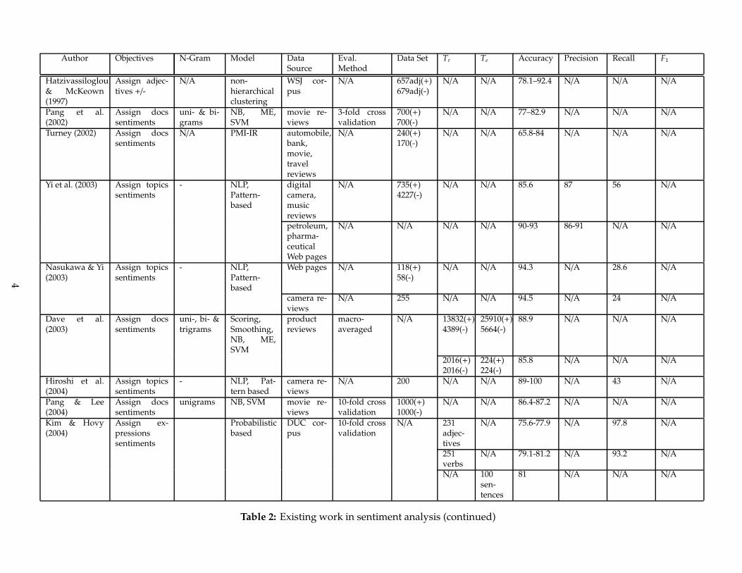
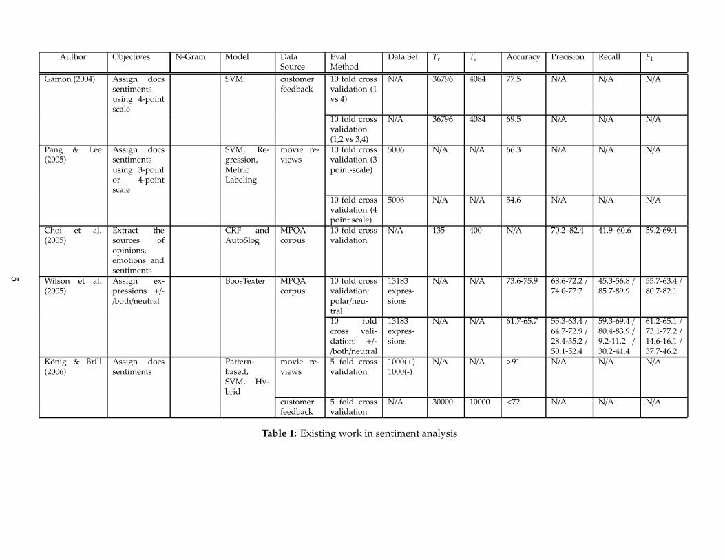
Table 2 lists some existing work in this area, and shows different types of objectives along with theassociatedmodels used and the experimental results produced. In an ideal scenario, all the experimentalresults are measured based on the micro-averaged and macro-averaged precision, recall, and F1 asexplained below.

2

Machine says yes Machine says no

human says yes tp fn

human says no fp tn

Table 1: A confusion table

Precision(P) =tp

tp+ f p ; Recall(R) =tp

tp+ f n ; Accuracy(A) =tp+tn

tp+tn+ f p+ f n ; F1 =2·P·RP+R

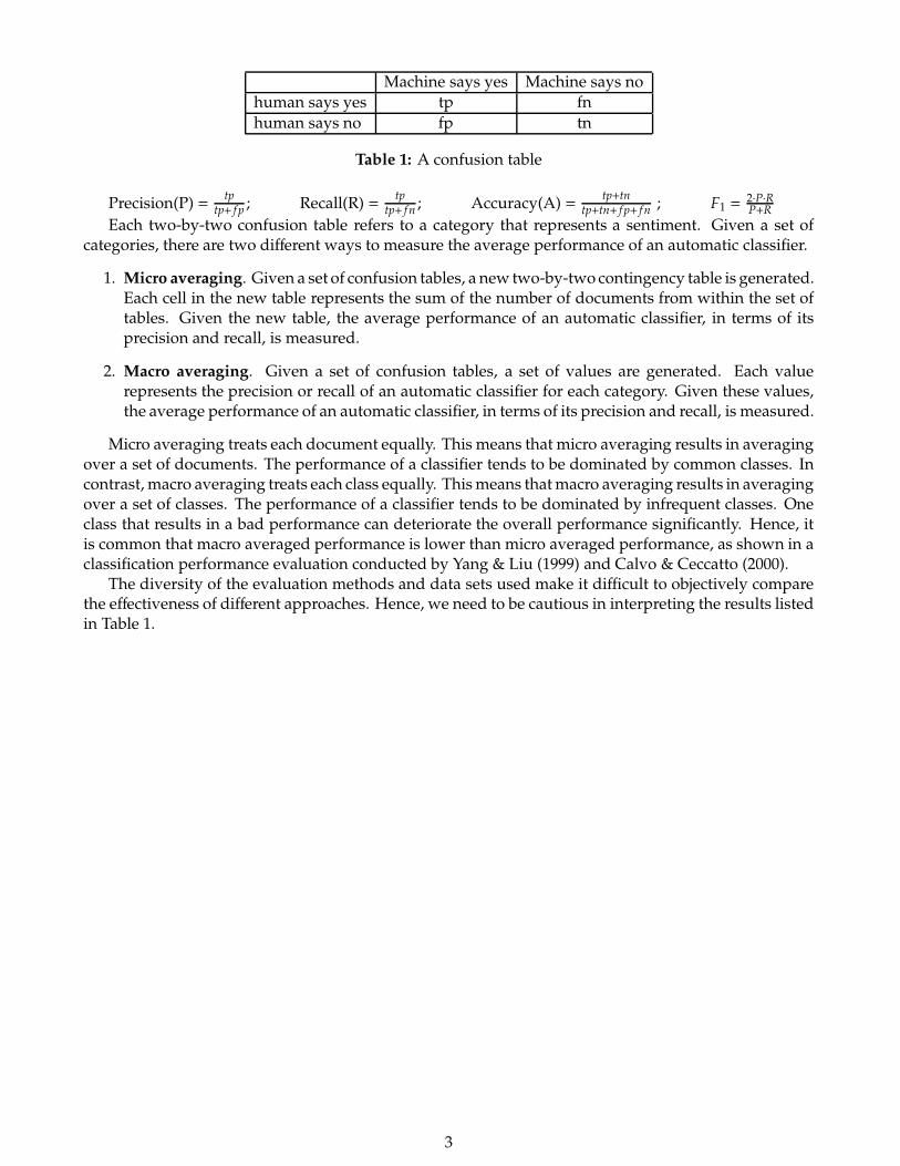
Each two-by-two confusion table refers to a category that represents a sentiment. Given a set ofcategories, there are two different ways to measure the average performance of an automatic classifier.

1. Micro averaging. Given a set of confusion tables, a new two-by-two contingency table is generated.Each cell in the new table represents the sum of the number of documents from within the set oftables. Given the new table, the average performance of an automatic classifier, in terms of itsprecision and recall, is measured.

2. Macro averaging. Given a set of confusion tables, a set of values are generated. Each valuerepresents the precision or recall of an automatic classifier for each category. Given these values,the average performance of an automatic classifier, in terms of its precision and recall, is measured.

Micro averaging treats each document equally. This means that micro averaging results in averagingover a set of documents. The performance of a classifier tends to be dominated by common classes. Incontrast, macro averaging treats each class equally. Thismeans thatmacro averaging results in averagingover a set of classes. The performance of a classifier tends to be dominated by infrequent classes. Oneclass that results in a bad performance can deteriorate the overall performance significantly. Hence, itis common that macro averaged performance is lower than micro averaged performance, as shown in aclassification performance evaluation conducted by Yang & Liu (1999) and Calvo & Ceccatto (2000).

The diversity of the evaluation methods and data sets used make it difficult to objectively comparethe effectiveness of different approaches. Hence, we need to be cautious in interpreting the results listedin Table 1.

3

Author Objectives N-Gram Model DataSource

Eval.Method

Data Set Tr Te Accuracy Precision Recall F1

Hatzivassiloglou& McKeown(1997)

Assign adjec-tives +/-

N/A non-hierarchicalclustering

WSJ cor-pus

N/A 657adj(+)679adj(-)

N/A N/A 78.1–92.4 N/A N/A N/A

Pang et al.(2002)

Assign docssentiments

uni- & bi-grams

NB, ME,SVM

movie re-views

3-fold crossvalidation

700(+)700(-)

N/A N/A 77–82.9 N/A N/A N/A

Turney (2002) Assign docssentiments

N/A PMI-IR automobile,bank,movie,travelreviews

N/A 240(+)170(-)

N/A N/A 65.8-84 N/A N/A N/A

Yi et al. (2003) Assign topicssentiments

- NLP,Pattern-based

digitalcamera,musicreviews

N/A 735(+)4227(-)

N/A N/A 85.6 87 56 N/A

petroleum,pharma-ceuticalWeb pages

N/A N/A N/A N/A 90-93 86-91 N/A N/A

Nasukawa & Yi(2003)

Assign topicssentiments

- NLP,Pattern-based

Web pages N/A 118(+)58(-)

N/A N/A 94.3 N/A 28.6 N/A

camera re-views

N/A 255 N/A N/A 94.5 N/A 24 N/A

Dave et al.(2003)


uni-, bi- &trigrams

Scoring,Smoothing,NB, ME,SVM

productreviews

macro-averaged

N/A 13832(+)4389(-)

25910(+)5664(-)

88.9 N/A N/A N/A

2016(+)2016(-)

224(+)224(-)

85.8 N/A N/A N/A

Hiroshi et al.(2004)

Assign topicssentiments

- NLP, Pat-tern based

camera re-views

N/A 200 N/A N/A 89-100 N/A 43 N/A

Pang & Lee(2004)


unigrams NB, SVM movie re-views


1000(+)1000(-)

N/A N/A 86.4-87.2 N/A N/A N/A

Kim & Hovy(2004)

Assign ex-pressionssentiments

Probabilisticbased

DUC cor-pus


N/A 231adjec-tives

N/A 75.6-77.9 N/A 97.8 N/A

251verbs

N/A 79.1-81.2 N/A 93.2 N/A

N/A 100sen-tences

81 N/A N/A N/A

Table 2: Existing work in sentiment analysis (continued)

4

Author Objectives N-Gram Model DataSource

Eval.Method

Data Set Tr Te Accuracy Precision Recall F1

Gamon (2004) Assign docssentimentsusing 4-pointscale

SVM customerfeedback

10 fold crossvalidation (1vs 4)

N/A 36796 4084 77.5 N/A N/A N/A

10 fold crossvalidation(1,2 vs 3,4)

N/A 36796 4084 69.5 N/A N/A N/A

Pang & Lee(2005)

Assign docssentimentsusing 3-pointor 4-pointscale

SVM, Re-gression,MetricLabeling

movie re-views

10 fold crossvalidation (3point-scale)

5006 N/A N/A 66.3 N/A N/A N/A

10 fold crossvalidation (4point scale)

5006 N/A N/A 54.6 N/A N/A N/A

Choi et al.(2005)

Extract thesources ofopinions,emotions andsentiments

CRF andAutoSlog

MPQAcorpus

10 fold crossvalidation

N/A 135 400 N/A 70.2–82.4 41.9–60.6 59.2-69.4

Wilson et al.(2005)

Assign ex-pressions +/-/both/neutral

BoosTexter MPQAcorpus

10 fold crossvalidation:polar/neu-tral

13183expres-sions

N/A N/A 73.6-75.9 68.6-72.2 /74.0-77.7

45.3-56.8 /85.7-89.9

55.7-63.4 /80.7-82.1

10 foldcross vali-dation: +/-/both/neutral

13183expres-sions

N/A N/A 61.7-65.7 55.3-63.4 /64.7-72.9 /28.4-35.2 /50.1-52.4

59.3-69.4 /80.4-83.9 /9.2-11.2 /30.2-41.4

61.2-65.1 /73.1-77.2 /14.6-16.1 /37.7-46.2

Konig & Brill(2006)


Pattern-based,SVM, Hy-brid

movie re-views


1000(+)1000(-)

N/A N/A >91 N/A N/A N/A

customerfeedback


N/A 30000 10000 <72 N/A N/A N/A

Table 1: Existing work in sentiment analysis

5

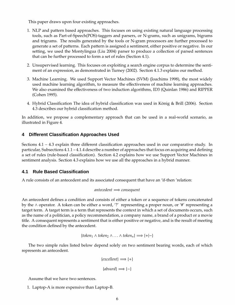
This paper draws upon four existing approaches.

1. NLP and pattern based approaches. This focuses on using existing natural language processingtools, such as Part-of-Speech(POS)-taggers and parsers, or N-grams, such as unigrams, bigramsand trigrams. The results generated by the tools or N-gram processors are further processed togenerate a set of patterns. Each pattern is assigned a sentiment, either positive or negative. In oursetting, we used the Montylingua (Liu 2004) parser to produce a collection of parsed sentencesthat can be further processed to form a set of rules (Section 4.1).

2. Unsupervised learning. This focuses on exploiting a search engine corpus to determine the senti-ment of an expression, as demonstrated in Turney (2002). Section 4.1.3 explains our method.

3. Machine Learning. We used Support Vector Machines (SVM) (Joachims 1998), the most widelyused machine learning algorithm, to measure the effectiveness of machine learning approaches.We also examined the effectiveness of two induction algorithms, ID3 (Quinlan 1986) and RIPPER(Cohen 1995).

4. Hybrid Classification The idea of hybrid classification was used in Konig & Brill (2006). Section4.3 describes our hybrid classification method.

In addition, we propose a complementary approach that can be used in a real-world scenario, asillustrated in Figure 4.

4 Different Classification Approaches Used

Sections 4.1 – 4.3 explain three different classification approaches used in our comparative study. Inparticular, Subsections 4.1.1 – 4.1.4 describe a number of approaches that focus on acquiring and defininga set of rules (rule-based classification). Section 4.2 explains how we use Support Vector Machines insentiment analysis. Section 4.3 explains how we use all the approaches in a hybrid manner.

4.1 Rule Based Classification

A rule consists of an antecedent and its associated consequent that have an ‘if-then ’relation:

antecedent =⇒ consequent

An antecedent defines a condition and consists of either a token or a sequence of tokens concatenatedby the ∧ operator. A token can be either a word, ‘?’ representing a proper noun, or ‘#’ representing atarget term. A target term is a term that represents the context in which a set of documents occurs, suchas the name of a politician, a policy recommendation, a company name, a brand of a product or a movietitle. A consequent represents a sentiment that is either positive or negative, and is the result of meetingthe condition defined by the antecedent.

{token1 ∧ token2 ∧ . . . ∧ tokenn} =⇒ {+|−}

The two simple rules listed below depend solely on two sentiment bearing words, each of whichrepresents an antecedent.

{excellent} =⇒ {+}

{absurd} =⇒ {−}

Assume that we have two sentences.

1. Laptop-A is more expensive than Laptop-B.

6

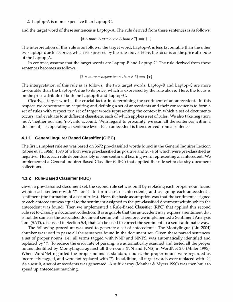
2. Laptop-A is more expensive than Laptop-C.

and the target word of these sentences is Laptop-A. The rule derived from these sentences is as follows:

{# ∧more ∧ expensive ∧ than∧?} =⇒ {−}

The interpretation of this rule is as follows: the target word, Laptop-A is less favourable than the othertwo laptops due to its price, which is expressed by the rule above. Here, the focus is on the price attributeof the Laptop-A.

In contrast, assume that the target words are Laptop-B and Laptop-C. The rule derived from thesesentences becomes as follows:

{? ∧more ∧ expensive ∧ than ∧ #} =⇒ {+}

The interpretation of this rule is as follows: the two target words, Laptop-B and Laptop-C are morefavourable than the Laptop-A due to its price, which is expressed by the rule above. Here, the focus ison the price attribute of both the Laptop-B and Laptop-C.

Clearly, a target word is the crucial factor in determining the sentiment of an antecedent. In thisrespect, we concentrate on acquiring and defining a set of antecedents and their consequents to form aset of rules with respect to a set of target words representing the context in which a set of documentsoccurs, and evaluate four different classifiers, each of which applies a set of rules. We also take negation,‘not’, ‘neither nor’and ‘no’, into account. With regard to proximity, we scan all the sentences within adocument, i.e., operating at sentence level. Each antecedent is then derived from a sentence.

4.1.1 General Inquirer Based Classifier (GIBC)

The first, simplest rule set was based on 3672 pre-classified words found in the General Inquirer Lexicon(Stone et al. 1966), 1598 of which were pre-classified as positive and 2074 of which were pre-classified asnegative. Here, each rule depends solely on one sentiment bearing word representing an antecedent. Weimplemented a General Inquirer Based Classifier (GIBC) that applied the rule set to classify documentcollections.

4.1.2 Rule-Based Classifier (RBC)

Given a pre-classified document set, the second rule set was built by replacing each proper noun foundwithin each sentence with ‘?’ or ‘#’ to form a set of antecedents, and assigning each antecedent asentiment (the formation of a set of rules). Here, the basic assumption was that the sentiment assignedto each antecedent was equal to the sentiment assigned to the pre-classified document within which theantecedent was found. Then we implemented a Rule-Based Classifier (RBC) that applied this secondrule set to classify a document collection. It is arguable that the antecedent may express a sentiment thatis not the same as the associated document sentiment. Therefore, we implemented a Sentiment AnalysisTool (SAT), discussed in Section 5.4, that can be used to correct the sentiment in a semi-automatic way.

The following procedure was used to generate a set of antecedents. The Montylingua (Liu 2004)chunker was used to parse all the sentences found in the document set. Given these parsed sentences,a set of proper nouns, i.e., all terms tagged with NNP and NNPS, was automatically identified andreplaced by ‘?’. To reduce the error rate of parsing, we automatically scanned and tested all the propernouns identified by Montylingua against all the nouns (NN and NNS) in WordNet 2.0 (Miller 1995).When WordNet regarded the proper nouns as standard nouns, the proper nouns were regarded asincorrectly tagged, and were not replaced with ‘?’. In addition, all target words were replaced with ‘#’.As a result, a set of antecedents was generated. A suffix array (Manber & Myers 1990) was then built tospeed up antecedent matching.

7

4.1.3 Statistics Based Classifier (SBC)

The Statistics BasedClassifier (SBC) used a rule set built using the following assumption. Bad expressionsco-occur more frequently with the word ‘poor’, and good expressions with the word ‘excellent’(Turney2002). We calculated the closeness between an antecedent representing an expression and a set ofsentiment bearing words. The following procedure was used to statistically determine the consequentof an antecedent.

1. Select 120 positive words, such as amazing, awesome, beautiful, and 120 negative words, such asabsurd, angry, anguish, from the General Inquirer Lexicon.

2. Compose 240 search engine queries per antecedent; each query combines an antecedent and asentiment bearing word.

3. Collect the hit counts of all queries by using the Google and Yahoo search engines. Two searchengines were used to determine whether the hit counts were influenced by the coverage andaccuracy level of a single search engine. For each query, we expected the search engines to returnthe hit count of a number of Web pages that contains both the antecedent and a sentiment bearingword. In this regard, the proximity of the antecedent and word is at the page level. A better levelof precision may be obtained if the proximity checking can be carried out at the sentence level.This would lead to an ethical issue, however, because we have to download each page from thesearch engines and store it locally for further analysis.

4. Collect the hit counts of each sentiment-bearing word and each antecedent.

5. Use 4 closeness measures to measure the closeness between each antecedent and 120 positivewords (S+) and between each antecedent and 120 negative words (S−) based on all the hit countscollected.

S+ =

120∑

i=1

Closeness(antecedent,word+i ) (1)

S− =

120∑

i=1

Closeness(antecedent,word−i ) (2)

If the antecedent co-occurs more frequently with the 120 positive words (S+ > S−), then this wouldmean that the antecedent has a positive consequent. If it is vice versa (S+ < S−), then the antecedenthas a negative consequent. Otherwise (S+ == S−), the antecedent has a neutral consequent. Thecloseness measures used are described below.

Document Frequency (DF). This counts the number of Web pages containing a pair of an an-tecedent and a sentiment bearing word, i.e., the hit count returned by a search engine. The largera DF value, the greater the association strength between antecedent and word. The use of DF in thecontext of automatic classification can be found in Yang & Pedersen (1997) and Yang (1999).

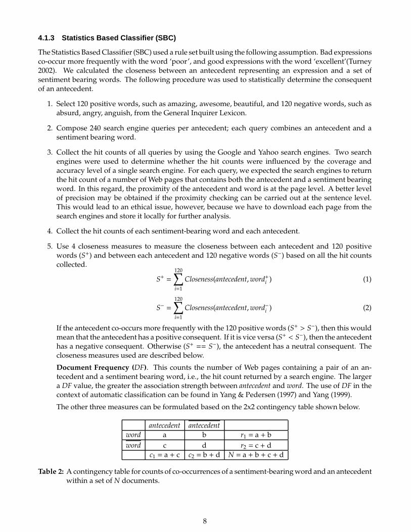
The other three measures can be formulated based on the 2x2 contingency table shown below.

antecedent antecedent

word a b r1 = a + b

word c d r2 = c + d

c1 = a + c c2 = b + d N = a + b + c + d

Table 2: Acontingency table for counts of co-occurrences of a sentiment-bearingword and an antecedentwithin a set of N documents.

8

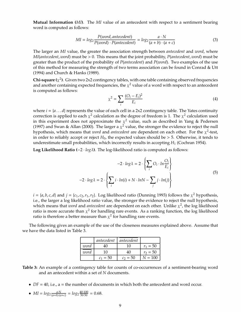
Mutual Information (MI). The MI value of an antecedent with respect to a sentiment bearingword is computed as follows:

MI = log2P(word, antecedent)

P(word) · P(antecedent)= log2

a ·N

(a + b) · (a + c)(3)

The larger an MI value, the greater the association strength between antecedent and word, whereMI(antecedent,word) must be > 0. This means that the joint probability, P(antecedent,word) must begreater than the product of the probability of P(antecedent) and P(word). Two examples of the useof this method for measuring the strength of two terms association can be found in Conrad & Utt(1994) and Church & Hanks (1989).

Chi-square (χ2). Given two 2x2 contingency tables, with one table containing observed frequenciesand another containing expected frequencies, the χ2 value of a word with respect to an antecedentis computed as follows:

χ2 =∑

i

(Oi − Ei)2

Ei(4)

where i = {a . . . d} represents the value of each cell in a 2x2 contingency table. The Yates continuitycorrection is applied to each χ2 calculation as the degree of freedom is 1. The χ2 calculation usedin this experiment does not approximate the χ2 value, such as described in Yang & Pedersen(1997) and Swan & Allan (2000). The larger a χ2 value, the stronger the evidence to reject the nullhypothesis, which means that word and antecedent are dependent on each other. For the χ2-test,in order to reliably accept or reject H0, the expected values should be > 5. Otherwise, it tends tounderestimate small probabilities, which incorrectly results in accepting H1 (Cochran 1954).

Log Likelihood Ratio (−2 · logλ). The log-likelihood ratio is computed as follows:

−2 · logλ = 2 ·

∑

i

Oi · lnOi

Ei

−2 · logλ = 2 ·

∑

i

i · ln(i) +N · lnN −∑

j

j · ln( j)

(5)

i = {a, b, c, d} and j = {c1, c2, r1, r2}. Log likelihood ratio (Dunning 1993) follows the χ2 hypothesis,i.e., the larger a log likelihood ratio value, the stronger the evidence to reject the null hypothesis,which means that word and antecedent are dependent on each other. Unlike χ2, the log likelihoodratio is more accurate than χ2 for handling rare events. As a ranking function, the log likelihoodratio is therefore a better measure than χ2 for handling rare events.

The following gives an example of the use of the closeness measures explained above. Assume thatwe have the data listed in Table 3.


word 40 10 r1 = 50

word 10 40 r2 = 50

c1 = 50 c2 = 50 N = 100

Table 3: An example of a contingency table for counts of co-occurrences of a sentiment-bearing wordand an antecedent within a set of N documents.

• DF = 40, i.e., a = the number of documents in which both the antecedent and word occur.

• MI = log2a·N

(a+b)·(a+c) = log240·10050·50 = 0.68.

9

• Prior to calculating the χ2, the expected frequencies, E are calculated.


word 25 25

word 25 25

Table 4: The expected frequencies, E.

χ2 =∑

i(Oi−Ei)

2

Ei= 36.

• Log likelihood ratio = 2 ·{

∑

i i · ln(i) +N · lnN −∑

j j · ln( j)}

= 38.55.

Both χ2 and log likelihood ratio strongly indicate that there is a sufficient evidence to reject H0. Thismeans that there is a degree of dependence between the antecedent and word.

4.1.4 Induction Rule Based Classifier (IRBC)

Given the two rule sets generatedby the Rule BasedClassifier (RBC) and Statistics BasedClassifier (SBC),we applied two existing induction algorithms, ID3 (Quinlan 1986) and RIPPER (Cohen 1995) providedby Weka (Witten & Frank 2005), to generate two induced rule sets, and built a classifier that could usethe two induced rule sets to classify a document collection.

These two induced rule sets canhint about howwell an induction algorithmworks onanuncontrolledantecedent set, in the sense that the antecedent tokens representing attributes are not predefined, butsimply derived from a pre-classified document set. The expected result of using an induction algorithmwas to have both an efficient rule set and better effectiveness in terms of both precision and recall.

4.2 Support Vector Machines

We used Support Vector Machine (SVMlight) V6.01 (Joachims 1998). As explained in Dumais & Chen(2000) and Pang et al. (2002) given a category set, C = {+1,−1} and two pre-classified training sets, i.e.,a positive sample set, T+r =

∑ni=1(di,+1) and a negative sample set, T−r =

∑ni=1(di,−1), the SVM finds a

hyperplane that separates the two sets with maximum margin (or the largest possible distance fromboth sets), as illustrated in Figure 1. At pre-processing step, each training sample is converted into a realvector, xi that consists of a set of significant features representing the associated document, di. Hence,Tr+ =

∑ni=1(xi,+1) for the positive sample set and Tr− =

∑ni=1(xi,−1) for the negative sample set.

10

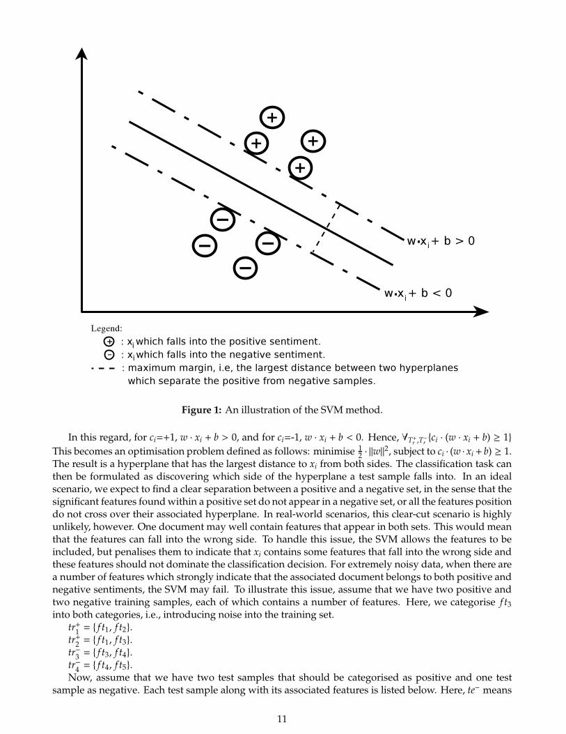
Figure 1: An illustration of the SVMmethod.

In this regard, for ci=+1, w · xi + b > 0, and for ci=-1, w · xi + b < 0. Hence, ∀T+r ,T−r {ci · (w · xi + b) ≥ 1}

This becomes an optimisation problem defined as follows: minimise 12 · ||w||

2, subject to ci · (w · xi + b) ≥ 1.The result is a hyperplane that has the largest distance to xi from both sides. The classification task canthen be formulated as discovering which side of the hyperplane a test sample falls into. In an idealscenario, we expect to find a clear separation between a positive and a negative set, in the sense that thesignificant features foundwithin a positive set do not appear in a negative set, or all the features positiondo not cross over their associated hyperplane. In real-world scenarios, this clear-cut scenario is highlyunlikely, however. One document may well contain features that appear in both sets. This would meanthat the features can fall into the wrong side. To handle this issue, the SVM allows the features to beincluded, but penalises them to indicate that xi contains some features that fall into the wrong side andthese features should not dominate the classification decision. For extremely noisy data, when there area number of features which strongly indicate that the associated document belongs to both positive andnegative sentiments, the SVM may fail. To illustrate this issue, assume that we have two positive andtwo negative training samples, each of which contains a number of features. Here, we categorise f t3into both categories, i.e., introducing noise into the training set.

tr+1= { f t1, f t2}.

tr+2= { f t1, f t3}.

tr−3= { f t3, f t4}.

tr−4= { f t4, f t5}.

Now, assume that we have two test samples that should be categorised as positive and one testsample as negative. Each test sample along with its associated features is listed below. Here, te− means

11

that the test sample should be categorised as negative, and te+ indicates positive.te+1= { f t1, f t2, f t4}. The sample contains two features that refer to positive sentiment, and only one

feature for negative sentiment (relatively noisy data).te+2= { f t1, f t2, f t4, f t5}. The sample contains features that refer to both positive andnegative sentiment

(a very noisy data).te−3= { f t3}. The sample only contains one feature that can refer to either positive or negative sentiment

(sparse and noisy data).The classification results are as follows: for te+

1, the SVM can correctly determine the side of the

hyperplane the test sample falls into, although it contains f t4. For the te+2and te−

3, the SVM fails to

correctly classify the samples due to a high level of ambiguity and sparseness in the test samples.In our setting, given a pre-classified document set, we automatically converted all the characters into

lower cases, and carried out tokenisation. Given all the tokens found, a set of significant features wasselected by using a feature selection method, i.e., document frequency as used by Pang et al. (2002), sothat we can compare our results with some existing results. As observed by Dumais & Chen (2000) andPang et al. (2002), to improve the performance of the SVM, the frequencies of all the features within eachdocument should be treated as binary and then normalised (document-length normalisation).

4.3 Hybrid Classification

Hybrid classification means applying classifiers in sequence. A set of possible hybrid classificationconfigurations is listed below.

1. RBC→ GIBC

2. RBC→ SBC

3. RBC→ SVM

4. RBC→ GIBC→ SVM

5. RBC→ SBC→ GIBC

6. RBC→ SBC→ SVM

7. RBC −→ SBC→ GIBC→ SVM

8. RBCinduced → SBC→ GIBC→ SVM

9. RBC→ SBCinduced → GIBC→ SVM

10. RBCinduced → SBCinduced → GIBC→ SVM

The rule set used by the RBCwas directly derived from a pre-classified document set, and had a highlevel of precision when it was applied to a test set. Hence, it was placed first. The antecedent set used bythe SBC was also directly derived from a pre-classified document set. Hence, the antecedent set had ahigh level of expressiveness, and was much better than the antecedent set used by the GIBC, which wasquite sparse. These are the reasons for the 2nd configuration. The SVM classifier was placed last becauseall the documents classified by the SVM were classified into either positive or negative. Hence, it didnot give another classifier the chance to carry out a classification once applied. The 7th configuration isthe longest sequence and applies all the existing classifiers. Based on the 7th configuration, the 8th − 10th

configurations were defined with respect to the two induced rule sets, discussed in Subsection 4.1.4, toevaluate the effectiveness of each induction algorithm used with respect to each induced rule set.

5 Experiment

This section describes the experiment and lists the experimental results.

12

5.1 Data

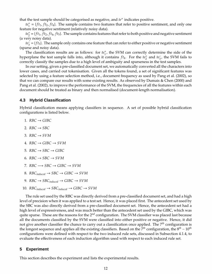
To evaluate the effectiveness of all the approaches used, we collected three sets of samples listed below.

Population Samples # of Features # of RBC Rules # of SBC Rules

1. Movie Reviews S1: 1000(+) & 1000(–) 44140 37356 35462

2. Movie Reviews S2: 100(+) & 100(–) 14627 3522 2033

3. Product Reviews S3: 180(+) & 180(–) 2628 969 439

4. MySpace Comments S4: 110(+) & 110(–) 1112 384 373

Table 5: The data sets

The second column refers to the number of pre-classified samples: 50% of which were classified intopositive and 50% as negative. The third column refers to the number of features extracted from thesample set (Section 4.2). The fourth column refers to the number of rules used by the RBC classifier(Section 4.1.2). This rule set was derived from a training set. The fifth column refers to the number ofrules used by the SBC classifier (Section 4.1.3). This rule set was derived from a test set that could not beclassified by the RBC.

The first data set was downloaded from Pang (2007). The second data set was a small version of thefirst data set, i.e., the first 200 samples extracted from the first data set. This small data set was requiredto test the effectiveness of the SBC and the induction algorithms (Section 4.1.4), which could not handlea large data set. The third data set was proprietary data provided by Market-Sentinel (2007). This is aclean data set that was pre-classified by experts. The fourth data set was also proprietary, provided byThelwall (2008), extracted from MySpace (2007), and preclassified by three assessors with kappa(κ) =100%, i.e. the three assessors completely agreed with each other. Whilst the movie review data containsa lot of sentences per document, the product reviews and MySpace comments are quite sparse.

5.2 Experimental Procedure

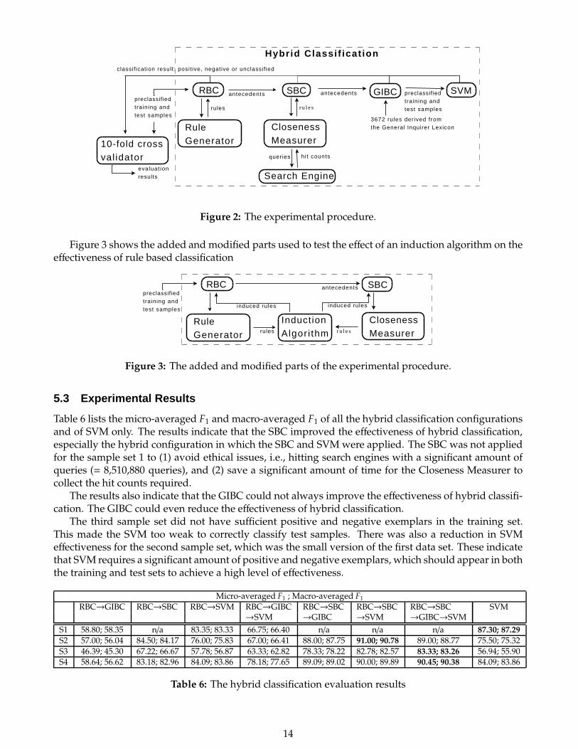
Figure 2 illustrates the experimental procedure. For each sample set, we carried out 10-fold crossvalidation. For each fold, the associated samples were divided into a training and a test set. For eachtest sample, we carried out a hybrid classification, i.e., if one classifier fails to classify a document,the classifier passes the document onto the next classifier, until the document is classified or no otherclassifier exists. Given a training set, the RBC used a Rule Generator to generate a set of rules and a setof antecedents to represent the test sample and used the rule set derived from the training set to classifythe test sample. If the test sample was unclassified, the RBC passed the associated antecedents ontothe SBC, which used the Closeness Measurer to determine the consequents of the antecedents. Prior toapplying a closeness measure for each antecedent, the Closeness Measurer submitted a set of queriesand collected the associated hit counts. If the SBC could not classify the test sample, the SBC passed theassociated antecedents onto the GIBC, which used the 3672 simple rules to determine the consequents ofthe antecedents. The SVMwas given a training set to classify the test sample if the three classifiers failedto classify it. The classification result was sent to and stored by the 10-fold cross validator to produce anevaluation result in terms of micro-averaged F1 and macro-averaged F1.

13

Hybr id Classi f icat ion

10-fold cross val idator

SBC GIBC

evaluat ionresults

preclassifiedtraining and test samples

RBC

Rule Generator

Closeness Measurer

Search Engine

rules

antecedents

r u l e s

queries hit counts

antecedents

3672 rules derived fromthe General Inquirer Lexicon

SVMpreclassifiedtraining and test samples

classif ication result: posit ive, negative or unclassif ied

Figure 2: The experimental procedure.

Figure 3 shows the added and modified parts used to test the effect of an induction algorithm on theeffectiveness of rule based classification

SBC preclassifiedtraining and test samples

RBC

rules

antecedents

r u l e s

Closeness Measurer

Rule Generator

Induction Algor i thm

induced rules induced rules

Figure 3: The added and modified parts of the experimental procedure.

5.3 Experimental Results

Table 6 lists the micro-averaged F1 and macro-averaged F1 of all the hybrid classification configurationsand of SVM only. The results indicate that the SBC improved the effectiveness of hybrid classification,especially the hybrid configuration in which the SBC and SVMwere applied. The SBC was not appliedfor the sample set 1 to (1) avoid ethical issues, i.e., hitting search engines with a significant amount ofqueries (= 8,510,880 queries), and (2) save a significant amount of time for the Closeness Measurer tocollect the hit counts required.

The results also indicate that the GIBC could not always improve the effectiveness of hybrid classifi-cation. The GIBC could even reduce the effectiveness of hybrid classification.

The third sample set did not have sufficient positive and negative exemplars in the training set.This made the SVM too weak to correctly classify test samples. There was also a reduction in SVMeffectiveness for the second sample set, which was the small version of the first data set. These indicatethat SVM requires a significant amount of positive and negative exemplars, which should appear in boththe training and test sets to achieve a high level of effectiveness.

Micro-averaged F1 ; Macro-averaged F1

RBC→GIBC RBC→SBC RBC→SVM RBC→GIBC RBC→SBC RBC→SBC RBC→SBC SVM→SVM →GIBC →SVM →GIBC→SVM

S1 58.80; 58.35 n/a 83.35; 83.33 66.75; 66.40 n/a n/a n/a 87.30; 87.29

S2 57.00; 56.04 84.50; 84.17 76.00; 75.83 67.00; 66.41 88.00; 87.75 91.00; 90.78 89.00; 88.77 75.50; 75.32

S3 46.39; 45.30 67.22; 66.67 57.78; 56.87 63.33; 62.82 78.33; 78.22 82.78; 82.57 83.33; 83.26 56.94; 55.90S4 58.64; 56.62 83.18; 82.96 84.09; 83.86 78.18; 77.65 89.09; 89.02 90.00; 89.89 90.45; 90.38 84.09; 83.86

Table 6: The hybrid classification evaluation results

14

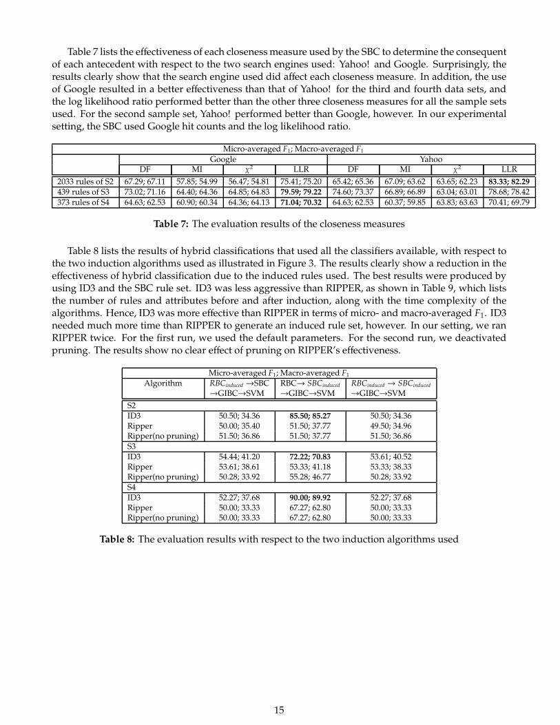
Table 7 lists the effectiveness of each closenessmeasure used by the SBC to determine the consequentof each antecedent with respect to the two search engines used: Yahoo! and Google. Surprisingly, theresults clearly show that the search engine used did affect each closeness measure. In addition, the useof Google resulted in a better effectiveness than that of Yahoo! for the third and fourth data sets, andthe log likelihood ratio performed better than the other three closeness measures for all the sample setsused. For the second sample set, Yahoo! performed better than Google, however. In our experimentalsetting, the SBC used Google hit counts and the log likelihood ratio.

Micro-averaged F1; Macro-averaged F1

Google YahooDF MI χ

2 LLR DF MI χ2 LLR

2033 rules of S2 67.29; 67.11 57.85; 54.99 56.47; 54.81 75.41; 75.20 65.42; 65.36 67.09; 63.62 63.65; 62.23 83.33; 82.29

439 rules of S3 73.02; 71.16 64.40; 64.36 64.85; 64.83 79.59; 79.22 74.60; 73.37 66.89; 66.89 63.04; 63.01 78.68; 78.42

373 rules of S4 64.63; 62.53 60.90; 60.34 64.36; 64.13 71.04; 70.32 64.63; 62.53 60.37; 59.85 63.83; 63.63 70.41; 69.79

Table 7: The evaluation results of the closeness measures

Table 8 lists the results of hybrid classifications that used all the classifiers available, with respect tothe two induction algorithms used as illustrated in Figure 3. The results clearly show a reduction in theeffectiveness of hybrid classification due to the induced rules used. The best results were produced byusing ID3 and the SBC rule set. ID3 was less aggressive than RIPPER, as shown in Table 9, which liststhe number of rules and attributes before and after induction, along with the time complexity of thealgorithms. Hence, ID3 was more effective than RIPPER in terms of micro- and macro-averaged F1. ID3needed much more time than RIPPER to generate an induced rule set, however. In our setting, we ranRIPPER twice. For the first run, we used the default parameters. For the second run, we deactivatedpruning. The results show no clear effect of pruning on RIPPER’s effectiveness.

Micro-averaged F1; Macro-averaged F1

Algorithm RBCinduced →SBC RBC→ SBCinduced RBCinduced → SBCinduced

→GIBC→SVM →GIBC→SVM →GIBC→SVM

S2ID3 50.50; 34.36 85.50; 85.27 50.50; 34.36Ripper 50.00; 35.40 51.50; 37.77 49.50; 34.96Ripper(no pruning) 51.50; 36.86 51.50; 37.77 51.50; 36.86



Table 8: The evaluation results with respect to the two induction algorithms used

15

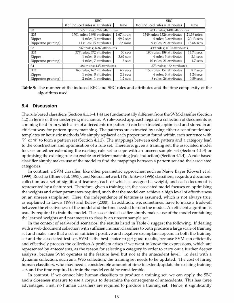
RBC SBC

# of induced rules & attributes time # of induced rules & attributes time

S2 3522 rules; 6799 attributes 2033 rules; 4404 attributes

ID3 1701 rules; 1698 attributes 1.67 hours 1349 rules; 1326 attributes 21.16 minsRipper 4 rules; 3 attributes 99.9 secs 4 rules; 3 attributes 20.13 secsRipper(no pruning) 11 rules; 15 attributes 1.32 mins 9 rules; 21 attributes 18.66 secs


ID3 377 rules; 372 attributes 30 secs 190 rules; 189 attributes 14.74 secsRipper 1 rules; 0 attributes 3.62 secs 4 rules; 3 attributes 2.1 secsRipper(no pruning) 4 rules; 7 attributes 3 secs 10 rules; 21 attributes 1.7 secs


ID3 163 rules; 162 attributes 6.9 secs 153 rules; 152 attributes 8.2 secsRipper 1 rules; 0 attributes 2.3 secs 4 rules; 3 attributes 1.24 secsRipper(no pruning) 2 rules; 1 attributes 1.2 secs 8 rules; 26 attributes 0.89 secs

Table 9: The number of the induced RBC and SBC rules and attributes and the time complexity of thealgorithms used

5.4 Discussion

The rule based classifiers (Section 4.1.1–4.1.4) are fundamentally different from the SVMclassifier (Section4.2) in terms of their underlyingmechanics. A rule-based approach regards a collection of documents asa mining field from which a set of antecedents (or patterns) can be extracted, optimised and stored in anefficient way for pattern-query matching. The patterns are extracted by using either a set of predefinedtemplates or heuristic methods.We simply replaced each proper noun found within each sentence with‘?’ or ‘#’ to form a pattern set (Section 4.1.2). The mappings between each pattern and a category leadto the construction and optimisation of a rule set. Therefore, given a training set, the associated modelfocuses on either extending the existing rule set to cope with an unseen sample set (Section 4.1.3) oroptimising the existing rules to enable an efficientmatching (rule induction) (Section 4.1.4). A rule-basedclassifier simply makes use of the model to find the mappings between a pattern set and the associatedcategories.

In contrast, a SVM classifier, like other parametric approaches, such as Naive Bayes (Govert et al.1999), Rocchio (Ittner et al. 1995), and Neural network (Yin & Savio 1996) classifiers, regards a documentcollection as a set of significant features, each of which is assigned a weight, and each document isrepresented by a feature set. Therefore, given a training set, the associated model focuses on optimisingthe weights and other parameters required, such that the model can achieve a high level of effectivenesson an unseen sample set. Here, the independence of features is assumed, which is not always true,as explained in Lewis (1998) and Belew (2000). In addition, we, sometimes, have to make a trade-offbetween the effectiveness of the model and the time needed to train the model. An efficient algorithm isusually required to train the model. The associated classifier simply makes use of the model containingthe learned weights and parameters to classify an unseen sample set.

In the context of real-world scenarios, the results listed in Table 6 suggest the following. If dealingwith aweb document collectionwith sufficient human classifiers to both produce a large scale of trainingset and make sure that a set of sufficient positive and negative exemplars appears in both the trainingset and the associated test set, SVM is the best choice to get good results, because SVM can efficientlyand effectively process the collection.A problem arises if we want to know the expressions, which arerepresented by antecedents, as the reason for selecting a category in order to carry out a further deeperanalysis, because SVM operates at the feature level but not at the antecedent level. To deal with adynamic collection, such as a Web collection, the training set needs to be updated. The cost of hiringhuman classifiers, who may need a considerable amount of time to extend/update the existing trainingset, and the time required to train the model could be considerable.

In contrast, if we cannot hire human classifiers to produce a training set, we can apply the SBCand a closeness measure to use a corpus to determine the consequents of antecedents. This has threeadvantages. First, no human classifiers are required to produce a training set. Hence, it significantly

16

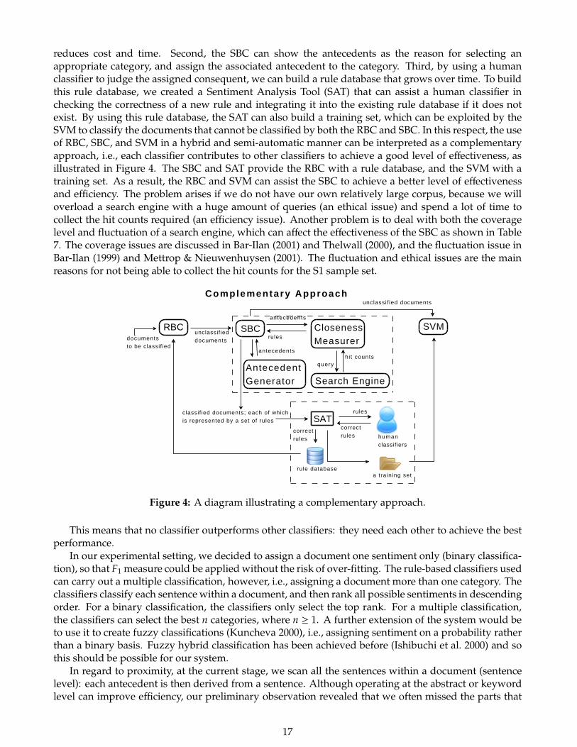
reduces cost and time. Second, the SBC can show the antecedents as the reason for selecting anappropriate category, and assign the associated antecedent to the category. Third, by using a humanclassifier to judge the assigned consequent, we can build a rule database that grows over time. To buildthis rule database, we created a Sentiment Analysis Tool (SAT) that can assist a human classifier inchecking the correctness of a new rule and integrating it into the existing rule database if it does notexist. By using this rule database, the SAT can also build a training set, which can be exploited by theSVM to classify the documents that cannot be classified by both the RBC and SBC. In this respect, the useof RBC, SBC, and SVM in a hybrid and semi-automatic manner can be interpreted as a complementaryapproach, i.e., each classifier contributes to other classifiers to achieve a good level of effectiveness, asillustrated in Figure 4. The SBC and SAT provide the RBC with a rule database, and the SVM with atraining set. As a result, the RBC and SVM can assist the SBC to achieve a better level of effectivenessand efficiency. The problem arises if we do not have our own relatively large corpus, because we willoverload a search engine with a huge amount of queries (an ethical issue) and spend a lot of time tocollect the hit counts required (an efficiency issue). Another problem is to deal with both the coveragelevel and fluctuation of a search engine, which can affect the effectiveness of the SBC as shown in Table7. The coverage issues are discussed in Bar-Ilan (2001) and Thelwall (2000), and the fluctuation issue inBar-Ilan (1999) and Mettrop & Nieuwenhuysen (2001). The fluctuation and ethical issues are the mainreasons for not being able to collect the hit counts for the S1 sample set.

Complementa ry Approach

SBC

Antecedent Generator

antecedents

ClosenessMeasurer

Search Engine

hit countsquery

antecedents

rules

classif ied documents; each of which is represented by a set of rules

rules

correctrules

rule database

documents to be classified

RBC SVMunclassified documents

human classifiers

SAT

a training set

unclassif ied documents

correctrules

Figure 4: A diagram illustrating a complementary approach.

This means that no classifier outperforms other classifiers: they need each other to achieve the bestperformance.

In our experimental setting, we decided to assign a document one sentiment only (binary classifica-tion), so that F1 measure could be applied without the risk of over-fitting. The rule-based classifiers usedcan carry out a multiple classification, however, i.e., assigning a document more than one category. Theclassifiers classify each sentencewithin a document, and then rank all possible sentiments in descendingorder. For a binary classification, the classifiers only select the top rank. For a multiple classification,the classifiers can select the best n categories, where n ≥ 1. A further extension of the system would beto use it to create fuzzy classifications (Kuncheva 2000), i.e., assigning sentiment on a probability ratherthan a binary basis. Fuzzy hybrid classification has been achieved before (Ishibuchi et al. 2000) and sothis should be possible for our system.

In regard to proximity, at the current stage, we scan all the sentences within a document (sentencelevel): each antecedent is then derived from a sentence. Although operating at the abstract or keywordlevel can improve efficiency, our preliminary observation revealed that we often missed the parts that

17

could lead us to a correct category. Another possibility thatwewould like to examine in the near future isto crystallise the process of sentiment categorization by analysing each paragraph/section, or by havinga modular domain ontology, which can allow a classifier to group relevant information together prior toassigning an appropriate sentiment. This will require a robust segmentation techniques and a conceptextraction algorithm that can make use of a set of domain ontologies.

In regard to the sample sets used, as explained in Section 5.1, two types of sample set were used:one that is a collection of long documents, and another of much shorter documents. The hybridclassification performed best for S2–S4. In our setting, we selected corpuses that may well containsentiment expressions or sentiment-bearing words because our aim is to evaluate different classificationapproaches used for sentiment analysis. Despite this limitation, we would argue that the combinationof rule-based classifiers and a SVM classifier in a hybrid manner is likely to also perform best for othertypes of samples because the defining factor is not the sentiment expressions or words, but a set of well-defined patterns and features that can lead to the construction of an optimal and efficient classificationmodel.

The use of the RIPPER algorithm resulted in a significant decrease in terms of micro- and macro-averaged F1 as shown in Table 8 due to its high level of aggression as shown in Table 9. In contrast, theuse of the ID3 algorithm decreased the effectiveness of the hybrid classification significantly less thanRIPPER, i.e., between 0.45 and 11.11 in terms of micro-averaged F1 and between 0.46 and 12.43 in termsof macro-averaged F1. The proportion of the ID3 reduction in terms of the number of reduced rules wasbetween 33.64% and 58.98%. Although this significant reduction only resulted in a slight decrease ineffectiveness, the induction algorithm generated a set of induced antecedents that are too sparse for adeeper analysis. In a real-world scenario, it is desirable to have two rule sets, one is the original set, andanother one is the induced rule set.

6 Conclusions

The use of multiple classifiers in a hybrid manner can result in a better effectiveness in terms of micro-and macro-averaged F1 than any individual classifier. By using a Sentiment Analysis Tool (SAT), wecan apply a semi-automatic, complementary approach, i.e., each classifier contributes to other classifiersto achieve a good level of effectiveness. Moreover, a high level of reduction in terms of the number ofinduced rules can result in a low level of effectiveness in terms of micro- and macro-averaged F1. Theinduction algorithm can generate a set of induced antecedents that are too sparse for a deeper analysis.Therefore, in a real-world scenario, it is desirable to have two rule sets, one is the original set, andanother one is the induced rule set.

Acknowledgements. Thework was supported by a European Union grant for activity code NEST-2003-Path-1 and the Future & Emerging Technologies scheme. It is part of the CREEN (Critical Events inEvolving Networks, contract 012684) and CyberEmotions projects. Wewould like to thankMark Rogersof Market Sentinel for help with providing classified data.

References

Bar-Ilan, J. (1999). Search engine results over time: A case study on search engine stability. Cybermetrics,2/3(1).

Bar-Ilan, J. (2001). Data collection methods on the Web for informetric purposes: A review and analysis.Scientometrics, 50(1), 7–32.

Belew, R. K. (2000). Finding out about - a cognitive perspective on search engine technology and the WWW.Cambridge University Press, 1st edition.

18

Calvo, R. A. & Ceccatto, H. A. (2000). Intelligent document classification. Intelligent Data Analysis, 4(5),411–420.

Choi, Y., Cardie, C., Riloff, E., & Patwardhan, S. (2005). Identifying sources of opinions with conditionalrandom fields and extraction patterns. In Proceeding of the conference on empirical methods in naturallanguage processing (EMNLP 2005), October 6–8, 2005 (pp. 355–362). Vancouver, B.C., Canada.

Church, K. W. & Hanks, P. (1989). Word association norms, mutual information and lexicography. InProceedings of the 27th annual meeting of the Association for Computational Linguistics (ACL), June 26–29, 1989(pp. 76–83). Vancouver, B.C.

Cochran, W. G. (1954). Some methods for strengthening the common χ2 tests. Biometrics, 10, 417–451.

Cohen, W. W. (1995). Fast effective rule induction. In A. Prieditis & S. Russell (Eds.), Proceedings of the12th international conference on machine learning (ICML 1995), July 9–12, 1995 (pp. 115–123). Tahoe City,California, USA.

Conrad, J. G. & Utt, M. H. (1994). A sytem for discovering relationships by feature extraction from TextDatabases. In W. B. Croft & C. J. van Rijsbergen (Eds.), Proceedings of the 17th annual international ACMSIGIR conference on research and development in information retrieval, July 3–6, 1994 (pp. 260–270). Dublin,Ireland.

Dave, K., Lawrence, S., & Pennock, D. M. (2003). Mining the peanut gallery: opinion extraction andsemantic classification of product reviews. In Proceedings of the 12th international WWW conference, May20–24, 2003 (pp. 519–528). Budapest, Hungary.

Dubitzky, W. (1997). Knowledge integration in case-based reasoning: a concept-centred approach. PhD thesis,University of Ulster.

Dumais, S.&Chen,H. (2000). Hierarchical classificationofWebcontent. InE.Yannakoudakis,N. J. Belkin,M.-K. Leong, & P. Ingwersen (Eds.), Proceedings of the 23rd annual international ACM SIGIR conference onresearch and development in information retrieval, July 24–28, 2000 (pp. 256–263). Athens, Greece.

Dunning, T. E. (1993). Accurate methods for the statistics of surprise and coincidence. ComputationalLinguistics, 19(1), 61–74.

Gamon, M. (2004). Sentiment classification on customer feedback data: noisy data, large feature vectors,and the role of linguistic analysis. In Proceedings of the 20th international conference on computationallinguistics (COLING 2004), August 23 – 27, 2004 (pp. 841–847). Geneva, Switzerland.

Govert, N., Lalmas, M., & Fuhr, N. (1999). A probabilistic description-oriented approach for categorisingWebdocuments. In S.Gauch& I.-Y. Soong (Eds.),Proceedings of the 8th international conference on informationand knowledge management (CIKM 1999), November, 1999 (pp. 474–482). Kansas City, USA.

Hatzivassiloglou, V. & McKeown, K. R. (1997). Predicting the semantic orientation of adjectives. InProceedings of the 8th conference on european chapter of the association for computational linguistics (pp. 174–181). Madrid, Spain.

Hiroshi, K., Tetsuya, N., & Hideo, W. (2004). Deeper sentiment analysis using machine translationtechnology. In Proceedings of the 20th international conference on computational linguistics (COLING 2004),August 23 – 27, 2004 (pp. 494–500). Geneva, Switzerland.

Ishibuchi, H., Nakashima, T., &Kuroda, T. (2000). A hybrid fuzzy gbml algorithm for designing compactfuzzy rule-based classification systems. The 9th IEEE International Conference on Fuzzy Systems, 2(706–711).

Ittner, D. J., Lewis, D. D., & Ahn, D. D. (1995). Text categorization of low quality images. In Proceedingsof the 4th annual symposium on document analysis and information retrieval (SDAIR 1995), April, 1995 (pp.301–315). Las Vegas, USA.

19

Joachims, T. (1998). Making large-scale SVM learning practical. In B. Scholkopf, C. J. C. Burges, & A. J.Smola (Eds.), Advances in kernel methods: support vector learning. The MIT Press.

Kim, S.-M.&Hovy, E. (2004). Determining the sentiment of opinions. InProceedings of the 20th internationalconference on computational linguistics (COLING 2004), August 23 – 27, 2004 (pp. 1367–1373). Geneva,Switzerland.

Konig, A. C. & Brill, E. (2006). Reducing the human overhead in text categorization. In Proceedings of the12th ACM SIGKDD conference on knowledge discovery and data mining, August 20–23, 2006 (pp. 598–603).Philadelphia, Pennsylvania,USA.

Kuncheva, L. I. (2000). Fuzzy Classifier Design. springer, 1st edition.

Lewis, D. D. (1998). Naive Bayes at forty: the independence assumption in information retrieval. InC. Nedellec & C. Rouveirol (Eds.), Proceedings of the 10th European conference on machine learning (ECML1998), April 21–24, 1998 (pp. 4–15). Chemnitz, Germany.

Liu, H. (2004). MontyLingua: An end-to-end natural language processor with common sense. Availableat < http : //web.media.mit.edu/ hugo/montylingua > (accessed 1 February 2005).

Manber, U. & Myers, G. (1990). Suffix arrays: a new method for on-line string searches. In Proceedingsof the first annual ACM SIAM symposium on discrete algorithms (SODA 1990), January 22–24, 1990. SanFrancisco, California.

Market-Sentinel (2007). Market Sentinel. <www.marketsentinel.com> (accessed 4 October 2007).

Mettrop,W.&Nieuwenhuysen,P. (2001). Internet search engines: Fluctuations indocument accessibility.Journal of Documentation, 57(5), 623–651.

Miller, G. A. (1995). WordNet: a lexical database for english. Communications of the ACM, 38(11), 39–41.

MySpace (2007). MySpace. <www.myspace.com> (accessed April 2007).

Nasukawa, T. & Yi, J. (2003). Sentiment analysis: capturing favorability using natural language process-ing. In Proceedings of the 2nd international conference on Knowledge capture, October 23–25, 2003. (pp. 70–77).Florida, USA.

Pang, B. (2007). Polarity data set v2.0. October 1997, <http://www.cs.cornell.edu/people/pabo/movie-review-data/> (accessed 4 August 2007).

Pang, B. & Lee, L. (2004). A sentimental education: sentiment analysis using subjectivity summarizationbased on minimum cuts. In Proceedings of the 42nd annual meeting of the Association for ComputationalLinguistics (ACL), July 21–26 , 2004 (pp. 271–278). Barcelona, Spain.

Pang, B. & Lee, L. (2005). Seeing stars: exploiting class relationships for sentiment categorization withrespect to rating scales. In Proceedings of the 43rd annual meeting of the Association for ComputationalLinguistics (ACL), June 25–30 , 2005 (pp. 115–124). University of Michigan, USA.

Pang, B., Lee, L., & Vaithyanathan, S. (2002). Thumbs up ? sentiment classification using machinelearning techniques. In Proceeding of the conference on empirical methods in natural language processing(EMNLP 2002), July 6–7, 2002 (pp. 79–86). Philadelphia, PA, USA.

Quinlan, J. R. (1986). Induction of decision trees. Machine Learning, 1, 81–106.

Sebastiani, F. (2002). Machine learning in automated text categorization. ACMComputing Surveys, 34(1),1–47.

20

Stone, P. J., Dunphy, D. C., Smith, M. S., & Ogilvie, D. M. (1966). The general inquirer: a computer approachto content analysis. The MIT Press.

Swan, R. & Allan, J. (2000). Automatic generation of overview timelines. In E. Yannakoudakis, N. J.Belkin, M.-K. Leong, & P. Ingwersen (Eds.), Proceedings of the 23rd annual international ACM SIGIRconference on research and development in information retrieval, July 24–28, 2000 (pp. 49–56). Athens, Greece.

Thelwall, M. (2000). Web impact factors and search engine coverage. Journal of Documentation, 56(2),185–189.

Thelwall, M. (2008). Fk yea I swear: Cursing and gender in a corpus of MySpace pages. Corpora, 3(1),83–107.

Turney, P. D. (2002). Thumbs up or thumbs down? semantic orientation applied to unsupervisedclassification of reviews. In Proceedings of the 40th annual meeting of the Association for ComputationalLinguistics (ACL), July 6–12 , 2002 (pp. 417–424). Philadelphia, PA, USA.

Wilson, T., Wiebe, J., & Hoffmann, P. (2005). Recognizing contextual polarity in phrase-level sentimentanalysis. In Proceeding of the conference on empirical methods in natural language processing (EMNLP 2005),October 6–8, 2005 (pp. 347–354). Vancouver, B.C., Canada.

Witten, I. H. & Frank, E. (2005). Data mining: practical machine learning tools and techniques. MorganKaufmann, San Francisco, 2nd edition.

Yang, Y. (1999). An evaluation of statistical approaches to text categorization. Information Retrieval,1(1–2), 69–90.

Yang, Y. & Liu, X. (1999). A re-examination of text categorization methods. In M. A. Hearst, F. Gey, & R.Tong (Eds.), Proceedings of the 22nd annual international ACM SIGIR conference on research and developmentin information retrieval, August 15–19, 1999 (pp. 42–49). Berkeley, USA.

Yang, Y. & Pedersen, J. O. (1997). A comparative study on feature selection in text categorization. InProceedings of the 14th international conference onmachine learning (ICML1997), July 8–12, 1997 (pp. 412–420).Nashville, Tennessee.

Yi, J., Nasukawa, T., Niblack, W., & Bunescu, R. (2003). Sentiment analyzer: extracting sentiments abouta given topic using natural language processing techniques. In Proceedings of the 3rd IEEE internationalconference on data mining (ICDM 2003), November 19–22, 2003 (pp. 427–434). Florida, USA.

Yin, L. L. & Savio, D. (1996). Learned text categorization by backpropagation neural network. Master’sthesis, Hong Kong University of Science and Technology.

21

Sentiment analysis: A combined · PDF fileSentimentAnalysis:ACombinedApproach Rudy Prabowo1,...

Documents

Transcript of Sentiment analysis: A combined · PDF fileSentimentAnalysis:ACombinedApproach Rudy Prabowo1,...