Sensitivity Analysis of the Extended AASHO Rigid Pavement Design Equation · ·...
59
Transcript of Sensitivity Analysis of the Extended AASHO Rigid Pavement Design Equation · ·...
SENSITIVITY ANALYSIS OF THE EXTENDED AASHO
RIGID PAVEMENT DESIGN EQUATION
by
Harvey J. Treybig Associate Design Engineer
Special Study 13.1
Research Section-Highway Design Division
TEXAS HIGHWAY DEPARTMENT
August 1969

ACKNOWLEDGEMENT
The idea for the research presented in this report came
about during the development of the rigid pavement design portion
of the Highway' Design Division Operations and Procedures Manual.
Suggestions offered by Mr. James L. Brown, Sr. Design Engineer at
the outset of this research are gratefully acknowledged.
This research was not entirely &"Upported by The Texas
Highway' Department. This report has been used by' the author as a
thesis for a masters degree; thus, it has required many hours
outside normal work time. The advice and counsel given by Dr. W. R.
Hudson and Dr. B. F. McCullough are gratefully acknowledged.
iii

Chapter
I.
II.
III.
IV.
TABLE OF CONTENTS
INTRODUCTION •
Objective.
Scope. • • •
THE PROBLEM AND APPROACH •
Selection of Model •
Approach •
FORMULATION OF DESIGN VARIABLE VARIATIONS ••
Development of Standard Deviations •
Concrete Properties
Slab Thickness •••••
Modulus of Subgrade Reaction. • •
Slab Continuity • • • •
Performance Variables
Discussion of Variables. • • . . . . Variations for Sensitivity Study.
RESULTS. • • • • • • •
Analysis •
Flexural Strength
Thickness •••
Slab Continuity.
Terminal Serviceability Index ••
Initial Serviceability Index ••
Modulus of Subgrade Reaction.
Modulus of Elasticity.. • • • •
iv
Page
1
2
2
3
3
4
11
11
11
12
12
13
13
14
15
19
19
25
25
25
25
29
29
29

Chapter
v. Discussion of Results .•••.
CONCLTJSIONS AND RECOMMENDATIONS ••.
Conclusions • •
Recommendations
APPENDICES
Appendix 1. Data for Deve1coment of Standard Deviations • •
Appendix 2. Development of a New Continuity Coefficient for Continu~us1y
Page
34
38
38
39
40
Reinforced Concrete Pavement 45
Appendix 3.
References • • •
Computer Program Listing •
• • • • • • • • • II! • • • @
48
51
v

Table
1
2
3
4
5
6
LIST OF TABLES
Variables and Levels for the Experiment.
Standard Deviations for Variables. • • • •
Deviation Levels of Independent Variables.
Percent Change in Total Traffic. • • • • •
Analysis of Variance for Expected Pavement Life. •
Order of Importance of Variables with Respect to Change in Expected Pavement Life ••••••••
Page
5
16
18
21
23
24
vi

LIST OF FIGURES
Figure No.
1 Factorial for Analysis of Change in Pavement Life ••
2 Graphical ExPlanation of Change in Expected Pavement
3
4
5
6
7
8
9
Life . . . . . . . . . .
Predicted Pavement Life in 18 Kip Equivalencies. • •
Effect of Flexural Strength Variations on Predicted Lire . . . . . . . . . . . . . CI • • • • • • 00 •
Effect of Thickness Variations on Predicted Life
Effect of Slab Continuity' Variations on Predicted Life . . .. . . . . . . . . . . . . . . . . . . . . .
Effect of Terminal Serviceability Index Variations on Predicted Life. • • • • • • • • • • • • • • • • •
Effect of Initial Serviceability Index Variations on Predicted Life. • • • .'. • • • • • • • • • • • •
Effect of Modulus of Subgrade Reaction Variations on Predicted Life. • • • • • • • • • • • • • • • • •
10 Effect of Modulus of Elasticity Variations on Pre-dicted Life. • • • • • • • • • • • • • • •
vii
Page
7
9
20
26
27
28
30
31
32
33

CHAPTER I
INTRODUCTION
The systems approach to pavement design has, since 1965, received
the attention of many researchers and design engineers. The use of
systems engineering has not developed any startling new inputs for the
solution of pavement design problem~ but rather organizes the various
aspects of the total problem into a manageable form. The systems concept
emphasizes those factors and ideas which are common to the successful
operation of relatively'independentparts of the whole pavement problem.
The output response of the pavement system (Ref. 1) is the
serviceability or performance that the pavement experiences. This
serviceability performance concept was first developed by' Carey' and Irick
(Ref. 2) at the AASHO Road Test. The AASHO Interim Guide for the Design
of Rigid Pavement Structures (Ref. 3) was the first design method which
incorporated the performance criteria.
The pavement design variables are of a stochastic nature.
Variations occur in the parameters which must be recognized by designers.
The effects of these stochastic variations are not alway's known. The
design variables usually considered in rigid pavement design are flexural
strength, modu:us of' elasticity, thickness, type of rigid pavement,
environmental conditions, expected traffic, monulus of subgrade reaction,
Poissons ratio, and subbase. All of these variables affect the problem
seriously.
1

Objecti ve
The objectives of this research are 1) to determine the
importance of rigid pavement design variables, 2) interactions among
the variables, and 3) to evaluate the effects of stochastic variations
for each variable using an extension of the AASHO Interim Guide (Ref 4).
Scope
The rigid pavement design variables considered are the modulus
of elasticity, flexural strength, slab thickness, slab continuity,
modulus of subgrade reaction, initial serviceability index and terminal
serviceability index. Each variable was evaluated for two levels
except the modulus of subgrade reaction at three levels and the initial
and terminal serviceability' indexes at one level each.
2

CHAPTER II
THE PROBLEM AND APPROACH
The evaluation of rigid pavement design variables requires
the use of some type of mathematical model relating the variables.
If a systems approach such as that of Hudson, et. al. (Ref 1) is to
ultimately be applicable to the model, then a system output response
~mch as performance must be included as a variable in the model.
Selection of Model
Pavement performance criteria was developed and used at the
AASHO Road Test, hence any design models developed using these per-
formance data could have been used in this study. Two mathematical
models for the rigid pavement design variables including the per-
J'ormance variable were considered. The first model is that from the
AASHO Interim Guide for the Design of Rigid Pavement Structures
(Ref 3). Realizing the shortcomings of the Interim Guide (Ref 3),
Hudson and McCullough (Ref 4) extended the Interim Guide (Ref 3) to
include modulus of elasticity, modulus of subgrade reaction, and a
term for pavement continuity to include continuously reinforced
concrete pavement.
Hudson and McCullough's extension of the Interim Guide was
selected for use in the study described here, because it was the best
available mathematical model based on performance which contained the
desired design variables. The model is as follows:
Log 2:W = - 9.483 - 3.837 log [_J~~ (1 _ 2.61a ~l G -----(1) Sx 02 Zl/403/4 )J + i3
:i.W = number of accumulated equivalent 18 kip single axle loads
3

J a coefficient dependent upon load transfer characteristics or slab continuity
Sx = modulus of rupture of concrete at 28 days (psi)
D = nominal thickness of concrete pavement (inches)
Z = E/k
E = modulus of elasticity for concrete (psi)
k = modulus of subgrade reaction (psi/inch)
a '" radius of equivalent loaded area = 7.15
G = log ~po - Pt J 'Po - 1.5
for Road _Test
Po = serviceability' index immediately' after construction
{3
Approach
terminal serviceability
= 1 + 1.624 x 10⁷
CD + 1) 8.46
index assumed as failure
A sensitivity analy'sis is a procedure to de'termine the change in
a dependen~ variable due to a unit change in an independent variable. A
sensitivity analysis can be used to evaluate a whole system of variables
and interactions between the variables that compose the system. The
rigid pavement design variables were evaluated in this research by means
of a sensitivity analysis which determined the change in pavement life
due to changes in the variables. However, the unit of study' for each
variable was chosen to represent statistical variations which have been
4
observed in actual engineering practice. The analysis involved the levels
of the variables shown in Table 1.
In a previous sensitivity study by' Buick, (Ref 5) the theoreti-
cal importance of design variables was evaluated by the use of an in-
stantaneous rate of change which was quantified by' first order partial
derivatives. Buick also evaluated the practical importance with a
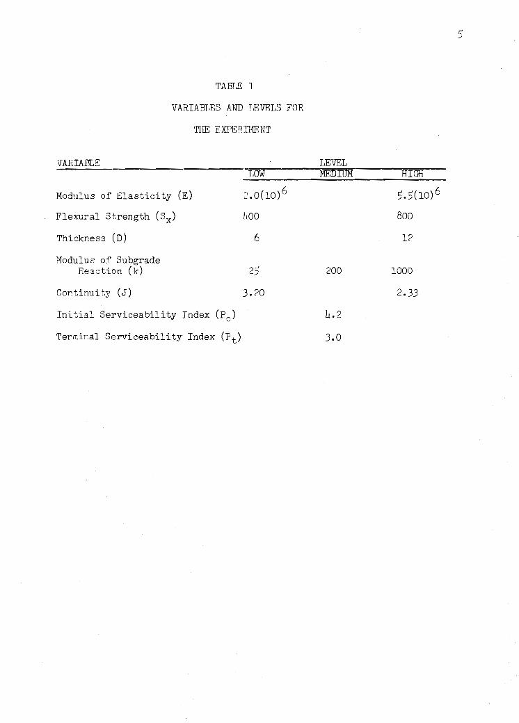
TABLE]
VARIABLES AND LEVELS FOR
THE EXPERTI1ENT
VARIABLE
Modulus of Elasticity (E)
Flexural Strength (Sx)
Thickness (D)
Modulus of Subgrade Reaction (k)
Continuity (J)
Initial Serviceability Index (po)
Terminal Serviceability Index (p t )
LOW
1,00
6
25
3.20
LEVEL MEDDJM HIGH
12
200 1000
2.33
4.2
3.0

tudy of U'e param8ter variations tolerated by r;elected thic'rre;~3 shange
constraints and a least squares fi'ting of appropriate equation3 to
parameter-thickness data.
In another sensitivity analysis McCullough, Van Til, Val.lerga,
and Hi ~kcl (Pef 6) formulated the ;1eressary partial derivatives but
used nlllrrnrj ca.l techniques to evaluate the lIerror!! in total traffic in
terms of percent change in each variable. McCullough, et. al. evaluat
ed only the AASHO Interim Guide (Ref J) while Buick evaluated the
AASHO Interim Guide Design Method, Corps of Engineers Rigid Pav€ment
Design Mettod for Streets and Roads, and the Portland Cement Associa
tion Design Method for Rigid Paveme'lts.
For this research a full factorial of the variables listed in
Table 1 was evaluated. In each factorial cell, each variable was
evaluated for the effect of its perturbations around the mean. In
order to compare meaningful variations of a variable, the standard
deviation was chosen rather than the standard unit change in the
variable.
Every material property, modulus of elasticity, flexural
strengtL, et.c., has a statistical distribution with a mean and
a variat.ion or a dispersion about tnis mean. Therefore, standard
deviadons have been developed for all the design variables to
characterize their variation. The development of these standard
deviation::; 1S covered in Chapter III.
6
The changes in expected pavement life have been computed for
variations in each variable in each block of the factorial (Figure 1).
Each block of the factorial involves a fixed level of the seven variables.

7
~ ~ 0+ ;;., .
./0 & q, :t-Q C<,> ~ 0 0 0
C 0Q'. . <S><s> Q. O¢' A,.. 400 2)0
C..(' 0<, "'0y>
¢<'>x" .,f>;' 6 6 ~p; c$l~ 12 12
25 1 13 25 37 ~ ,.-... 200 2 14 26 38 0 r-l '-" (\J 1000 3 15 27 39
0 C\J .
25 4 16 28 40 (Y\
@ -200 5 17 29 41
I~ 1000 6 18 30 42
25 7 19 31 43 fo I 44 ",-... 200 8 20 32 0 r-l '-" C\J 1000 9 2l 33 45
(Y\ (Y\ .
-0 25 10 22 34 46 C\J ,.... 0 r-l 200 11 23 35 47 .... ~
1.f\ . 1.1\ 1000 12 24 36 43
FACTORIAL FOR ANALYSIS OF CHANGE
IN PAVEr1ENT LIFE
Figure 1
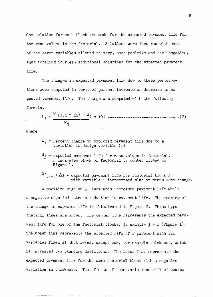
One solution for each block was [,l.'lde for the expected pavemer,t life for
the mean values in the factorial. Solutions were then run with each
of the seven variables allowed t" vary, once positive and ::'01:-; negative,
thus to-l:,aling fourteen additionc.l solutions for the expected pavement
life.
The changes in expected pavement life due to these perturba-
tions were computed in terms of percent increase or decrease in ex-
pected pavement life. The change was computed with the fallowing
formula.
Where
Li W (j,i ~ ~)~j x 100 --------------------------------(2) Wj
= Percent change in expected pavement life due to a variation in design variable (i)
w .. = J expected pavement life for mean values in factorial.
j indicates block of factorial by' number listed in Figure 1.
W(j,i ~~) = expected pavement life for factorial blor.k j
8
with variable 1 incremented plus or minus some change.
A positive sign on Li indicates increased pavement life while
a negative sign indicates a reduction in pavement life. The meaning of
the change in expected life is illustrated in Figure 2. Three hypo-
thetical lines are shown. The center line represents the expected pave-
ment life for one of the factorial blocks, j, example j = 1 (Figure 1).
The upper line represents the expected life of a pavement with all
variables fixed at that level, except one, for example thickness, which
is increased two standard deviations. The lower line represents the
expected pavement life for the same factorial block with a negative
variation in thickness. The effects of some variations will of course

(j) ~
Wj ·ri H
~
s:: (j)
E (j) :> eel
0...
'0 (j) +' U (l,) 0.. ><
f:i1
Positive change W(j, i +/:::.) j '" 1 i = thickness
t::. '" 0.33 in / /
--__ -_____________ -___ 1 _____ -/
/ /
/ / / /
/ .,// / /'/
/ .,/ / /'
/ // i'/
Time
/ /
t
GRAPHICAJ~ EXPLANATIO[~ OF G:r!ANGE IN
EXPECTED PAVEMENT LIFE
Figure 2
W for j = 1 All mean values
Negative change W(j, i -l!..) j = 1 i ::::: thickness
D,. = 0.33 in

be reversed, that is an increase in the variable gives a decreased
life.
10

CHAPTER III
FORMULATION OF DESIGN VARIABLE VARIATIONS
Highway contractors in general do not use statistical quality
control in construction. Thus there is little exact data on expected
variations in the design variables. The two largest sources of data
for the development of the standard deviations are the permanent
construction files of the Texas Highway' Department and the reports
on the AASHO Road Test. The author's experience also aided iIi the
development of some of the standard deviations. A search of the
literature yielded little more than what was available through the
above mentioned sources.
Development of Standard Deviations
Using available data together with some assumptions, standard
deviations were developed for each level of each variable selected
for this investigation (Table 1).
Concrete Properties. Two properties of concrete are of inter-
est in this study: 1) the modulus of elasticity (E) and 2) the
flexural strength (Sx)' The two levels of modulus of elasticity were
2.0 x 10⁶ psi and 5.5 x 10⁶psi • Test data for modulus of elasticity'
were obtained from Shafer of the Texas Highway Department (Ref 7) and
from ,Johnson!s work (Ref 8) at the Iowa Engineering Experiment Sta-
tion. Analysis of these data yielded standard deviations of 0.2 x
106 psi and 0.6 x 10⁶ psi respectively, for the low and high levels
of modulus of elasticity (Appendix 1).
Two levels of flexural strength are involved, 400 psi and
800 psi. Data related to variation of flexural strength were
11

obtained from several sources. The Texas Highway Department maintains
permanent files of flexural strength on all concrete paving projects.
From these records (Ref 9) much data was used. Hudson has extended
some of the AASHO Road Test Work (Ref 10) wherein flexural strength
data were also available. Schleider reviewed large amounts of flex
ural strength data from the Texas Highway Departments construction
files (Ref 11). Data for the high level, 800 psi came from all three
sources and the average standard deviation was 60 psi. The data for
the low level of flexural strength came only from Schleider (Ref 11).
The standard deviation for the low level was 45 psi.
Slab Thickness (D). Slab thickness was involved at two levels,
6 inches and 12 inches. Sample data were obtained for several other
thicknesses from the Texas Highway Department (Ref 9), but were not
available for these thicknesses. From. these data (See Appendix 1),
the average coefficient of variation was obtained. The coefficient of
variation was assumed to be constant. The standard deviations for
the two thicknesses in this experiment were computed using the obtained
coefficient of variation. They are 0.165 inch and 0.330 inch for the
six and twelve inch slab thicknesses, respectively.
Modulus of Subgrade Reaction (k). Although k-values are used in
design, records show little evidence that agencies designing and build
ing pavements actively measure modulus of subgrade reactions by use of
plate load tests (Ref 6). However, data were available from the AASHO
Road Test (Ref 10). These data were for k-values averaging about 100
pci. The standard deviation for this data was 16 pci. In this in
vestigation,k-values of 25, 200, and 1000 were used. Thus, the
12

assumption was again made that the coefficient of variation would be
a constant over a range of values of the parameter. The three
necessary standard deviations were computed using the coefficient of
variation, 15 percent, (See Appendix 1) from the AASHO data. The
standard deviations calculated for the three levels were 4, 30, and
150 pci, respectively (Appendix 1).
Slab Continuity (J). The slab continuity term was used by
Hudson and McCullough to characterize the particular type of.rigid
pavement being considered. Hudson and McCullough found J = 2.20 for
continuously' reinforced concrete pavement. This value was based on
Texas Highway Department design procedures and pavement performance.
Since that time McCullough and Treybig (Ref 12) have conducted
extensive studies on deflection of jointed and continuously reinforced
concrete pavement. This research has yielded a new J-value for
continuous pavement, J = 2.33 (Appendix 2). Since this term is not
a measureable material property but a pavement characteristic, its
dispersion could not be determined in the normal way. Based on
variability of deflection measurements and experience, standard dev
iations were estimated as 0.19 for continuous pavement and 0.13 for
jointed pavement.
Performance Variables (po' Pt ). In this design method,
performance is a function of the serviceability indexes. The initial
serviceability index at time of construction has never been evaluated
for rigid pavements other than those at the AASHO Road Test. Scrivner
(Ref 13) indicated that the average initial serviceability index on
flexible pavement in Texas is 4.2. Having no better estimate for
13

Texas, this same value was assumed fer rigid pavement for this fltudy.
Performance studies by Treybig (Ref 14) indicate that the initial
serviceability index of in-service pavements is well below the 4.5
measured at the AASHO Road Test (Ref 15). Based on a knowledge of
construction variability and numerous observations of pavements under
construction together with comments by Hudson and McCullough (Ref 16),
the standard deviation of the initial serviceability index was
estimated to be 0.5.
For the standard deviation of the terminal serviceability
index, actual measurements of serviceability index were used. Measure
ments at the AASHO Road Test (Ref 15) as well as performance st~dies
in Texas indicate a standard deviation of 0.3.
Discussion of Variables
The standard deviations developed for each of the design
variables cannot all be used with the same confidence. Those that are
true standard deviation developed from real data are thought to be
good estimates of variation in service. These include the modulus of
elasticity, flexural strength, and the terminal serviceability index.
For both the modulus of subgrade reaction and thickness the
assumption was made that the coefficient of variation for each of the
two respective variables would be constant for all levels ~f the
variables in the ranges under study. Since the thickness data th'l.t
were used (Ref 9) gave reasonable standard deviations and also a rea
ably constant coefficient of variation over the range, the standard
deviations for the thicknesses in this experiment are believed to he
reasonable. The coefficient of variation on the k-value resulted
14

from data recorded at the AASHO Road Test (Ref 10) which was conduct
ed under somewhat more careful control than might be expected in
the field. Furthermore, there is little data to substantiate the
assumption of constant coefficient of variation, although wide var
iations would not be expected. The values used herein should be
verified in future studies.
The standard deviations of the remaining two variables are
associated with a somewhat lower level of confidence. The standard
deviations for both the initial serviceability index and the J
value are estimated and not computed from numerical data.
Variations for Sensitivity Study
Each of the design variables has some distribution. For
the analysis of changes in expected pavement life the total variation
for each variable was either one or two standard deviations. Table
2 indicates the levels of each variable as well as the respective
standard deviations.
The variation in modulus of elasticity was selected as plus
or minus one standard deviation.
The variation selected for thickness, flexural strength, and
modulus of subgrade reaction was plus or minus two standard deViations,
since 95 percent of the total variation (assuming a normal distri
bution for each variable) would be included within the bounds.
The level of variation for slab continuity was selected as
plus or minus one standard deviation since the variation was esti
mated rather than based on real data.
15

TABLE 2
STANDARD DEVIATIONS FOR VARIABLES
VARIABLE
Modulus of Elasticity (E)
Flexural Strength (Sx)
Thickness (D)
Modulus of Subgrade Reaction (k)
Continuity (J)
Initial Serviceability Index (po)
Terminal Serviceability Index (P t )
LEVEL
2.0(10)6
5'.5'(10)6
400 800
6 12
25' 200
1000
3.20 2.33
4.2
3.0
16
STANDARD DEVIATION
0.2(10)6
0.6(10)6
45' 60
0.165' 0.330
4 30
15'0
0.13 0.19
0.5'
0.3

The serviceability parameters were both varied plus and minus
one standard deviation. The initial serviceability index has an
17
upper limit of 5.0; thus, with a mean of 4.2 and two standard deviations,
unreasonable answers would result. For the terminal serviceability
index, plus and minus one standard deviation was also selected.
The deviation levels of all variables are listed in Table 3.

18
TABLE 3
DEVIATION LEVELS OF INDEPENDENT VARIABLES
Variable Level Deviation Level
Modulus of Elasticity (E) 2(10)6 1.8(10)~ 2.2(10)
5.5(10)6 4.9(10)~ 6.1(10)
Flexural Strength (Sx) 400 305 495
800 680 920
Thickness (D) 6 5.67 6.33
12 11.34 12.66
Modulus of Subgrade Reaction (k) 25 17 33
200 140 260
1000 700 1300
Continuity (J) 3.20 3.07 3.22
2.33 2.14 2.52
Initial Serviceability Index (po) 4.2 3.7 4.7
Terminal Serviceability Index (Pt ) 3.0 2.7 3.3

CHAPTER TV
RESULTS
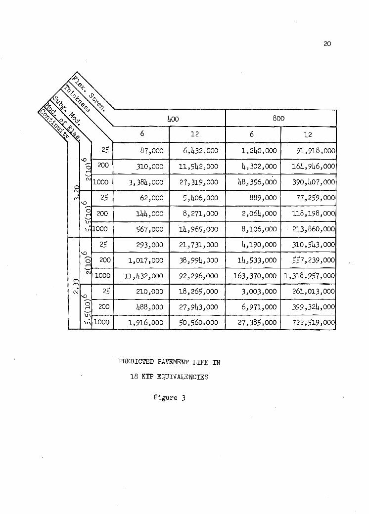
The total expected pavement life as predicted by' equation
(1) has been determined for the factorial. Figure 3 shows the
predicted pavement life for each case in total 18 kip single axle
applications. The effects of positive and negative variations in
each of the variables in each factorial block have been evaluated
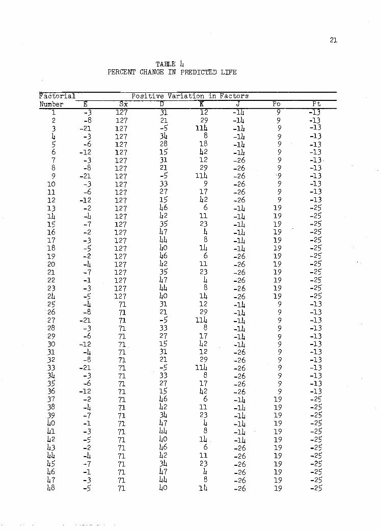
in terms of percent change in life. Table 4 contains the percent
change in life for variations in each variable in each respective
factorial block.
Analysis
An analysis of variance was made on the mean values of the
expected pavement life shown in Figure 3. The analysis of variance
considered only' five of the seven factors since the initial and
terminal serviceability' indexes were studied only at one level.
Those factors and interactions found to be significant at
selected alpha levels are shown in Table 5. All other possible in
teractions were found insignificant.
A graphic presentation was chosen to relate the effects of
variations in each variable to pavement life. Pavement life change
is characterized by the percent change in the summation of traffic
loads for the performance period. The performance period is the time
required for the pavement serviceability index to decrease from 4.2
to 3.0. Table 6 contains the factors analyzed in their order of
importance with respect to change in life due to factor variations.
19
~ ~ \S)+ ~.(. .
U¢ 0+.., ~t ... ~ \s)<s> \S).,
V. ~Q'" <s>. 0.,. '* ~. ° 0cy
~¢ ~. ~.(.
t. . 25
...0
C 200 :: N 1000
~ (V' 25
\.()
-q 200
I ~ \.. ,;, 1000
25 \.()
0 200 .-l
OJ 1000 rt; rt; .
25 N \.() .--.. 0 200 .-l '-' l.r\ .
1000 'If\
400
6 12
87,000 6,432,000
310,000 11,542,000
3,384,000 27,319,000
62,000 5,406,000
144,000 8,271,000
567,000 14,965,000
293,000 21,731,000
1,017,000 38,994,000
11,432,000 92,296,000
210,000 18,265,000
488,000 27,943,000
1,916,000 50,560.000
PREDICTED PAVEMENT LIFE IN
18 KIP EQUIVALENCIES
Figure 3
20
800
6 12
1,240,000 91,918,000
4,302,000 164,946,000 .
48,356,000 390,407,000
889,000 77 ,259,000
2,064,000 118,198,000
8,106,000 213,860,000
4,190,000 310,543,000
14,533,000 557,239,000
.163,370,000 1,318,957,000
3,003,000 261,013,000
6,971,000 399,324,000
27,385,000 722,519,000
21
TABLE 4 PERCENT CHANGE IN PREDICTED LIFE
Factorial Positive Variation in Factors Number E Sx D I{ J Po Pt
1 -3 127 31 12 -14 9 -13 2 -8 127 21 29 -14 9 -13 3 -21 127 -5 114 -14 9 -13 4 -3 127 34 8 -14 9 -13 5 -6 127 28 18 -14 9 -13 6 -12 127 15 42 -14 9 -13 7 -3 127 31 12 -26 9 -13 8 -8 127 21 29 -26 9 -13 9 -21 127 -5 114 -26 -9 -13
10 -3 127 33 9 -26 9 -13 11 -6 127 27 17 -26 9 -13 12 -12 127 15 42 -26 9 -13 13 -2 127 46 6 -14 19 -25 14 -4 127 42 11 -14 19 -25 15 -7 127 35 23 -14 19 -25 16 -2 127 47 4 -14 19 -25 17 -3 127 44 8 -14 19 -25 18 -5 127 40 14 -14 19 -25 19 -2 127 46 6 -26 19 -25 20 -4 127 42 11 -26 19 -25 21 -7 127 35 23 -26 19 -25 22 -1 127 47 4 --26 19 -25 23 -3 127 44 8 -26 19 -25 24 -5 127 40 14 -26 19 -25 25 -4 71 31 12 -14 9 -13 26 -8 71 21 29 -14 9 -13 27 -21 71 -5 114 -14 9 -13 28 -3 71 33 8 -14 9 -13 29 -6 71 27 17 -14 9 -13 30 -12 71 15 42 -14 9 -13 31 -4 71 31 12 -26 9 -13 32 -8 71 21 29 -26 9 -13 33 -21 71 -5 114 -26 9 -13 34 -3 71 33 8 -26 9 -13 35 -6 71 27 17 -26 9 -13 36 -12 71 15 42 -26 9 -13 37 -2 71 46 6 -14 19 -25 38 -4 71 42 11 -14 19 -25 39 -7 71 34 23 -14 19 -25 40 -1 71 47 4 -14 19 -25 41 -3 71 44 8 -14 19 -25 42 -5 71 40 14 -14 19 -25 43 -2 71 46 6 -26 19 -25 44 -4 71 42 11 -26 19 -25 45 -7 71 34 23 -26 19 -25 46 -1 71 47 4 -26 19 -25 47 -3 71 44 8 -26 19 -25 48 -5 71 40 14 -26 19 -25

22
TABLE 4 Cont.
Factorial Negative Variation in Factors Number E Sx D K J Po Pt
1 5 -65 -25 -14 17 -14 11 2 10 -65 -18 -26 17 -14 11 3 33 -65 +12 -54 17 -14 11 4 3 -65 -26 -10 17 -14 11 5 8 -65 -22 -17 17 -14 11 6 16 -65 -12 -33 17 -14 11 7 4 -65 -25 -13 39 -14 11 8 10 -65 -18 -26 39 -14 11 9 33 -65 +12 -54 39 -14 11
10 3 -65 -26 .. 54 39 -14 . 11 11 7 -65 -22 -18 39 -14 11 12 16 -65 -12 -33 39 -14 11 13 2 -65 -33' -7 17 -28 25 14 5 -65 -30 -12 17 -28 25 15 8 -65 -26 -21 17 -28 25 16 2 -65 -33 -5 17 -28 25 17 3 -65 -32 -9 17 -28 25 18 6 -65 -29 -15 39 -28 25 19 2 -65 -33 -7 39 -28 25 20 4 -65 -30 -12 39 -28 25 21 8 -65 -26 -21 39 -28 25 22 2 -65 -33 -5 39 -28 25 23 3 -65 -32 -9 39 -28 25 24 6 -65 -29 -15 39 -28 25
. 25 4 -46 -25 -13 17 -14 11 26 10 -46 -18 -26 17 -14 11 27 33 -46 +12 -54 17 -14 11 28 3 -46 -26 -10 17 -14 11 29 7 -46 -22 -18 17 -14 11 30 16 -46 -12 -33 17 -14 11 31 4 -46 -25 -13 39 -14 11 32 10 -46 -18 -26 39 -14 11 33 33 -46 +12 -54 39 -14 11 34 3 -46 -26 -10 39 -14 11 35 7 -46 -22 -18 39 -14 11 36 16 -46 -13 -33 39 -14 11 37 2 -46 -33 -7 17 -28 25 38 4 -46 -30 -12 17 -28 25 39 8 -46 -26 -21 17 -28 25 40 2 -46 -33 -5 17 -28 25 41 3 -46 -32 -9 17 -28 25 42 6 -46 -29 -15 39 -28 25 43 2 -46 -33 -7 39 -28 25 44 4 -46 -30 -12 39 -28 25 45 8 -46 -26 -21 39 -28 25 46 2 -46 -33 -5 39 -28 25 47 3 -46 -32 -9 39 -28 25 48 6 -46 -29 -15 39 -28 25

TABLE 5
ANALYSIS OF VARIANCE FOR EXPECTED PAVEMENT LIFE
Combination Degrees of of Factors Freedom
5 1 4 1
4x5 1 1 1
1x5 1 1x4 1
1x4x5 1 3 2
3x4 2 3x5 2
3x4x5 2 2 1
1x3 2 1x3x4 2
2x5 1 2x3 2
1x3x5 2 2x3x4 2
Legend of Factors
1 - Continuity 2 - Modulus of Elasticity 3 - Modulus of Subgrade Reaction 4 - Flexural Strength 5 - Thickness
Mean F Squares Value -
44,961,433 161.1 43,452,302 155.7 33,969,002 121. 7 16,971,287 60.8 13,267,448 47.5 12,822,076 45.9 10,023,472 35.9
8,946,193 32.0 6,758,959 24.2 5,269,082 18.9 3,980,810 14.3 3,605,810 12.9 2,639,904 9.5 1,994,450 7.2 1,740,530 6.2 1,601,046 5.7 1,554,808 5.6 1,209;627 4.3
23
Significance Level, ~
1 1 1 1 1 1 1 1 1 1 1 1 1 5 5 5 5 5

TABLE 6
ORDER OF IMPORTANCE OF VARIABLES WITH RESPECT
TO CHANGE IN EXPECTED PAVEMENT LIFE
FLEXURAL STRENGTH
THICKNESS
CONTINUITY
TERMINAL SERVICEABILITY INDEX
INITIAL SERVICEABILITY INDEX
MODULUS OF SUBGRADE REACTION
MODULUS OF ELASTICITY
24

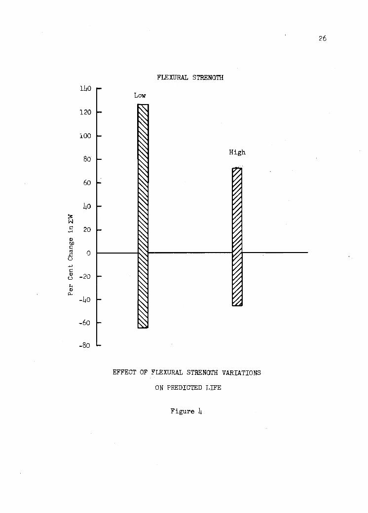
Flexural Strength. The change in predicted accumulated traffic
or pavemdnt life is more severe for the lower level of strength or
lightweight concrete (Figure 4). The change in life due to variation
in flexural strength is independent of the concrete modulus of
elasticity, thickness, modulus of subgrade reaction and slab continuity.
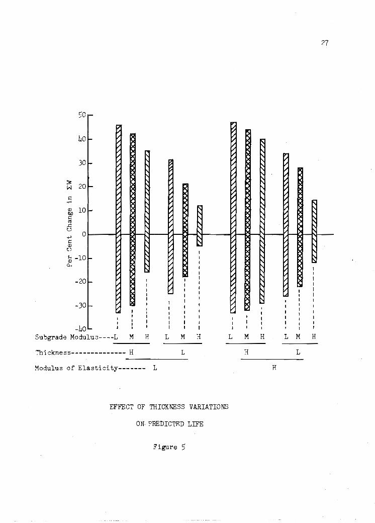
Thickness. The changes in pavement life due to variations
in thickness are shown in Figure 5. The positive variations in thick
ness resulted in longer life while thinning the slab shortened the
predicted life. The change in life which results from thickness varia
tions is independent of the continuity and nexural strength but de
pendent on the concrete modulus of elasticity, modulus of subgrade
reaction and thickness. The changes in life due to positive variations
in thickness are greater per standard deviation than that due to
negative changes (Figure 5).
Slab Continuity_ Variations in slab continuity show that the
change in expected pavement life is greater for continuously reinforced
concrete pavement than for jointed concrete. The change in expected
pavement life due to variations in continuity of the slab is indepen
dent of all factors that were evaluated at more than one level. In
actual highway engineering practice this independence may be con
jectured, but for the mathematical model used herein the indepen-
dence does exist. Figure 6 shows the effects of variations in
continuity' on the change in expected pavement life for both jointed
and continuously reinforced concrete pavement.
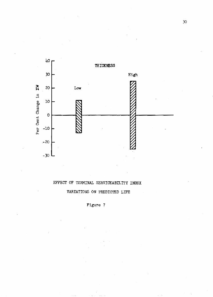
Terminal Servi~eability Index. One level of terminal service
ability index, 3.0, was evaluated. The change in' expected pavement
life is dependent only on the level of thickness and is more severe at
25
140
120
100
80
60
40 ::: w c 20 .,-l
(1) bD C ctI 0 ..c
0
+> s:: (1) -20 0
~ (1)
p...
-40
-60
-80
FLEXURAL STRENGTH
Low
High
EFFECT OF FLEXURAL STRENGTH VARIATIONS
ON PREDICTED LIFE
Figure 4
26
27
50 ..-
40
30
~ 20 V.J
c .~
Q) 10 bD C n:l
..c::: (.)
.;..:> 0 c Q)
(;.)
@ -10 Cl..
-20
-30
-40
Ii ~ L-' ~ I- 1/ V ~ ~ 1/ 1/ ~ ~ ~ II
f-. 1/ ~ ~ I' II ~
[..i
iI ~ II ~ ~ ~ ~ ~ ~ ~
i- ~ II II 1\ ~ ~ ~
I' V 1/ 1\ 1/
~ 1/ II 1\ 1/ 1/
~ ~ ~ II i- II II 1/
1/ 1/ II 1\ 1/ 1/ 1/ t-. II 1/ 1/ V " II ~ V II " ~ I' 1/ t-
Il ~ ~ ~ 1/
" II II
~ II ... II ~ II ~
~ ~ I v- II " l- V I ~ 1\ II ~ ~ " ~ I I' II
~ ~ ~ t ~ ~ I>C
I I
~ 1/ ~ I
II I ~ t I 1..-,
i- I/ I I I II V ~ I
~ V I
~ I I I
I it I
I I ~ L.i I I V I I
~ ~ I I I I
fo- 1/ I I I ~ I II I I V , I I
I • I I 1.01 • I I .... I I I
I I I I I I ,
I I I I I I I
I I I I I I I I I I I I
'- I I I I I I I I I , I
Su'bgrade Modulus----L M E L M H L M H L M H
Thickness-------------- H L H L
Modulus of Elasticity------- L H
EFI''ECT OF THICKNESS VARIATIONS
ON, PREDICTED LIFE
Figure ;)

c ",..,
3)
20
10
Contin1.lou-31y Reinforced
Jointed
O~------~ ~------------------~ A---------------+J C Cll u -10 ~ Cll
p..,
-20
-30
EFFECT OF SLAB CONTINUITY VARIATIONS
ON PREDICTED LIFE
Figure 6

the higher level of thiokness as related in Figure 7.
Initial Servioeabi1itz Index. All work in this experiment
was for one level of the initial serviceability index, 4.2. It was
found that change in expected pavement life due to variations in the
initial serviceability index depends only on the level of thickness.
The change in expected life is independent of all other factors in
the inference as shown in Figure 8 where the change in life for var
iations in the initial serviceability index is greater for the high
level of thickness.
Modulus of SubgradeReaction. The changes in pavement life
due to variations in k-va1ue are dependent on the level of the
variable, modulus of elasticity and thickness as shown in Figure 9.
It is independent of the level of flexural strength or the slab
continuity. For the two lower levels of the subgrade modulus, the
positive and negative changes in expected life are approximately
equal, while for the high level of the subgrade modulus they are not.
The changes in expected pavement life due to variations in the modulus
of subgrade reaction are much higher for the lower level of thickness
than for the higher level of thickness.
Modulus of Elasticity. The change in expected pavement life
is positive for a decrease and negative for an increase in the modulus
of elasticity (Figure 10). The magnitude of change in life is depen
dent on the level of the concrete modulus, the pavement thickness,
and the modulus of subgrade reaction, but is independent of flexural
strength and slab continuity.
29
30
40 THICKNESS
.30 High
~ 20 Low
s:: • .-1
(\) 10 bD s:: ttl ..c u 0 ~ s:: (\) u ~ -10 (\)
p..
-20
-.30
EFFECT OF TERMINAL SERVICEABILITY INDEX
VARIATIONS ON PREDICTED LIFE
Figure 7

31
30 'mICKNESS
~ High
H 20 c Low .....
J 10
+> O~------~~~----------------~~r-------------ijj t)
~ -10 CL..
-20
-30
EFFECT OF INITIAL SERVICEABTI.ITY INDEX
VARIATIONS ON PREDICTED LIFE
Figure 8

32
50
40
114 r-
-~ '\ r-
'" ~ ~ " 30
20 :.;: H
10 ;:::
.,-l
(]) tlO 0 ;::: til .l:! (.)
+' -10 ;::: (])
(.)
~ (]) -20 p..
-30
-40
-50
-60
~ ~ ~
~ " " ~ ~ ~
~ ~ 1\ ~ r-~ r--..
~ ~ ~ ~ V t'- ~ ~ ~ ~ ~ ~ t'-II t'- ~ !i1 ~ V
:\ V
" ~ ~ ~ 1\
" 17 1\ '" / " ~ / t\_
~ ~ "- ~ ,I
~ 1\ >< ~ \
~ t'-
~ .. " \ ;..-~
1\ ~ \
~ \ 1\ II ~ I l- I " II I ~ ~ I :::!I 1\ ~ ~ I I I I · 1\ I [\ I
~ ~ I I :'\ I , 1\ • ~ I I • I
" I I r-. I l"- I • I , I I I ~ I I' l- I b. l"- I I I I
I ~ • I , :'\ I I
i' I I I I [\ I • • I I I I I I ,
I I I II i' I I I I' I I I I I • " I
I I
" I I , I
P- I I I
I I I I I
~ I I I
" I , I I I I I
" I I I I I I I I I I . I • I I I I
" I I I • I I I I
" I I \ I I · , I , I I , I I
, \ I ~ • I • I " I J I I · I I I I ." I I I • I I I I I · , I I I
" I I , I · I · I I I I
" I I I i I I I I I I I I I 1\ I I
, I I I I I I I I I I 1\ I I I I I l- I I I I I I • I I I ... I I I • • I I I I I I I I I , I I I t!:I I I · I ,
I I I I I I
I I I I I · I I I I I . I I , · I I • I I , I ... , , I I I I I I I , I I
Subgrade Modulus--L M H L M L M H L M H
Thickness---- ... ------- H L H L
Modulus of Elasticity------ L H
EFFECT OF MODULUS OF SUBGRADE REACTION
VARIATIONS ON PREDICTED LIFE
Figure 9

15
~ H
s:: -.--I
Q) b.O s:: ~ ..c: 0
(.)
+' r.:: Q)
(.)
~ Q) p..
-15
-20
-25 Subgrade Modulus---- L
I
M
Thickness--------------- H
H
Modulus of Elastici ty---------- L
I
L M H L
L
EFFECT OF MODULUS OF ELASTICITY
VARIATIONS ON PREDICTED LIFE
Figure 10
, M H
H
H
I
L
, I .
M H
L
33

Discussion of Results
Examination of the data in Figure 3 indicates that the design
equation CEq. 1) predicts extremely high estimates of the total
pavement life or accumulated traffic when combinations of variables
occur at the high level. These results alone are not meaningful. The
percent change in pavement life due to variations in the factors
over this entire range is useful in evaluating the importance of
factors. The use of a digital computer made it a relatively simple
matter to evaluate the full factorial experiment.
The analysis of variance for these data has indicated eight
two-factor interactions and five three-factor interactions to be
significant. Thus variations in expected pavement life other than that
due to ~he main factors was not random, but was due to a relationship
between the factors. The analy-sis of variance thus indicates for the
extended AASHO design equation for rigid pavement ~hat the design
variables are truly significant as well as the combinations or inter
actions cited in Table 5. The analysis of variance yielded essentially
the same ordering on the design variables as did the analysis of changes
in expected pavement life for factor variations.
According to AASHO Road Test results (Ref 15), the average
absolute residual for the total expected traffic is about ten per
cent; thus, computed changes in the expected pavement life or total
traffic of ten percent or less have little or no meaning.
As expected and as indicated by this study the two most
significant factors in the extended AASHO rigid pavement design equation
(Table 5 and Figure 4 and 5) are the flexural strength and the pave-
34

ment thickness. The analysis of variance for the mean values of
expected pavement life also showed the thickness and flexural strength
to be very important (Table '). These two are closely followed by
the slab continuity term. Buick, in his "Analysis and Synthesis of
Highway Pavement Design" (Ref ,) found that for the AASHO rigid pave
ment design method, the flexural strength was one of the two most
important parameters. McCullough, et. ale (Ref 6) also found the
effects of flexural strength highly significant. Thus it appears
logical that variations in the flexural strength shJuld also be
highly significant in the extension of the AASRO rigid pavement
design method. Under actual construction conditions the flexural
strength of the concrete has a high probability of variation (Ref 6).
The magnitude of change in expected pavement life is not equal for
equal magnitude positive and negative variations in the flexural
strength (Figure 4).
The expected change in pavement service life due to over
estimated or deficiences in thickness was over 20 percent in most
cases (Figure '). The study by McCullough, (Ref 6) also indicates
the thickness to be a very significant factor. The chance for
variation in thickness is always present during construction where
a section might be built thicker or thinner than the desired plan
dimensions. The magnitude of change in expected pavement is
not equal for equal magnitude positive and negative variations in
thickness.
The slab continuity factor in this design equation does no
thing more than designate the type of rigid pavement. In actual
3,

construction the continuity of continuously reinforced pavement would
certainly depend on the percent longitudinal steel, concrete strength
and probably several other parameters. The continuity of a jointed
pavement would certainly depend on joint spacings and mechanical
load transfer supplied. Thus the continuity or load transfer term
might be somewhat misleading. The variations in the load transfer
term show what might be expected in practice due to construction
variations as well as variation in material properties.
36
Variations in the serviceability' factors showed significant
changes in the traffic service life. They were not as great as the
flexural strength or the thickness, but greater than 10 percent, the
average absolute residual on total traffic (Ref 15) required for signifi
cance. This design method indicates the change in life due to
variations in the serviceability parameters to be dependent on thick
ness. Buick, (Ref 5) in his evaluation of relative practical
importance which parallels this experiment, found the serViceability
parameters to be less important than flexural strength which agrees
with the findings herein.
The numerical evaluation of changes in expected pavement
life in terms of percent change in total traffic shows that of the
variables in the design equation, variations in the modulus of
elasti:::ity of the concrete have the least effect on the pavement
service life within reasonable variations. Except for the high levels
of modulus of subgrade reaction on the low level of thickness, all
changes in expected life (Figure 10), positive or negative, are less
than ten percent. This confirms McCullough!s'finding (Ref 6). Another factor whose variations showed insignificant effects
was the modulus of subgrade reaction. For the factorial of this
experiment only' the variations at the high level of the subgrade
modulus created significant changes (10%) in the expected traffic
service life. This corroborates the McCullough work.
37

Conclusions
CHAPTER. Tl
CONCLUSIONS AND RECOMMENDATIONS
This investigation was conducted to determine the sensitivity
of pavement life as predicted by practical variations in the design
variables. The conclusions are limited to the range of variables
studied in this experiment and are of course only as good as the
model being investigated. These findings however can provide reason
able information for use in design in selecting those variables which
require the most intensive study effort, those which promise to yield the
best improvements. This study illustrates a method which can be used
to set priorities to upgrade any' design model.
Based on the premise that the more important factors produce
a greater change in the expected pavement life, the following con
clusions are warranted.
1. The flexural strength and thickness are the most important
factors whose negative variations may critically shorten
pavement life.
2. The continuity factor was found to be the third most
important factor.
3. The terminal and initial serviceability indexes were
found to be important factors whose variations produce
significant changes in the expected pavement life.
4. The modulus of sub grade reaction and the modulus of
elasticity are the least important design factors "Those
variations do not significantly affect the expected pave-
38
..

ment life.
5. Significant interactions between the design factor8 do
occur indicating that the variations in the pavement life
are not completely defined by the design variables alone.
Furthermore this study shows those variables where tighter quality
control restrictions are needed in order to improve life estimates.
Recommendations
Based on this investigation, it is recommended that:
1. Practicing highway' engineers recognize that variations in
the pavement variables are real and have a significant
effect on pavement life and that better quality control
of concrete flexural strength and thickness be incorporated
to improve pavement performance.
2. Roughness specifications of new pavements should be updated
to obtain smoother pavement and higher initial service
ability' indices.
3. In future model development attention should be given to
these variables in the priority listing presented.
39
APPENDIX 1
DATA FOR DEVELOPMENT
OF STANDARD DEVIATIONS
40

FLEXURAL STRENGTH
High Level
Standard Deviations
From Texa s Highway 60 Dept. (Ref. 9) 46
70 Hudson (Ref. 10) 45
From Schleider (Ref. 11) 82 56
Average Standard Deviation = 60 psi.
Low Level
Standard Deviations
From Schleider (Ref. 11) 67 20
Average Standard Deviation = 45 psi.

MODULUS OF ELASTICITY
Shafer*(Ref. 7)
2.11 x 10⁶
2.31 x 10⁶
1.96 x 10⁶
1.88 x 10⁶
2.33 x 10⁶
2.43 x 10⁶
2.26 x 10⁶
Mean = 2.183 x 10⁶ psi
Low Level
Johnson (Ref. 8)
2.62 x 10⁶
2.65 x 10⁶
6 2.99 x 10
2.90 x 10⁶
3.12 x 10⁶
Mean = 2.856 x 10⁶psi
42
Standard Deviation e 0.194 x 10⁶psi Standard Deviation = 0.217 x 10⁶ psi
Average Standard Deviation for low level = 0.2 x 10⁶ psi
High Level
Shafer-!} (Ref. 7)
4.19 x 10⁶
5.81 x 10⁶
5.21 x 10⁶
5.84 x 10⁶
5.68 x 10⁶
5.99 x 10⁶
, Mean = 5.453 x 10⁶ psi Standarj Deviation = 0.633 x 10⁶ psi
Standard Deviation selected for high level = 0.6 x 10⁶ psi
~} Average of three values

THICKNESS
From Texas Highway Department (Ref. 9)
Thickness Standard Deviation (in)
8 - CRCP 0.229
8 - CRCP 0.227
8 - CRCP 0.2.36
8 - JCP 0.21,
9 - JCP 0 • .3.36
10 - JCP 0.298
Mean coeffi~ient of variation = 2.7,
Assume coefricient of variation constant
for all thicknesse~ thus the standard
deviations ror the low and high levels are:
D = 6 in
D "" 12 in tr = 0.330
Coefficient of Variation
2.7
2.7
2.8
2.6
.3"
2.9
4.3
/'

MOOULUS OF SUBGRADE REACTION
From !ASHO Road Test (Ref. 10)
OU ter Wheel Pa th Inner Wheel Pa th
94
107
85
124
113
78
107
105
122
Mean· 104
Standard Deviation = 16.8
Coefficient of Variation = 16.1%
101
103
85
117
135
97
123
113
Mean =: 109
Standard Deviation = 15.9
Coefficient of Variation • 14.6%
Average coefficient of variation = 15%
Assume coefficient of variation constant
for all valUes of modulus of subgrade reaction.
Thus for this experiment the standard deviations
for each level of k-va1ue are:
level k-va1ue Standard Deviation -low 25 4
medium 200 30
high 1000 150
44

APPENDIX 2
DEVELOPMENT OF A NEW CONTINUITY
COEFFICIENT FOR CONTINUOUSLY REINFORCED
CONCRETE PAVEMENT
45

DEVELOPMENT OF A NEW CONTINUITY COEFFICIENT FOR
CONTINUOUSLY REINFORCED CONCRETE PAVEMENT
The IIJII term which is a coefficient dependent on load transfer
characteristics or slab continuty came about in Hudson and McCullough's
extension of the AASHO Rigid Guide. It was part of Spang1ers stress
equation which was used to modify the original AASHO equation (Ref. 17).
The value of J for jointed pavement was 3.2. For continuously rein-
forced concrete pavemen~Hudson and McCullough made J = 2.2 based on
comparisons of previous design procedures and performance studies.
In 1968 McCullough and Treybig completed a comprehensive rigid
pavement denection study (Ref. 12) which included both continuously
reinforced and jointed concrete pavements. This research provided data
for revision of the value of J for continuously' reinforced pavement.
The new value of J is based on the relative differences in deflections
of eight inch pavements.
For continuously reinforced concrete pavements,the difference
in edge deflection was noted for measurements made at and midway
between shrinkage cracks. The same type data were developed for joint-
ed pavements with edge deflections measured at joints and midway
between. The percent difference in each of the two respective measure-
ments was used in a ratio to compute J for continuous pavement as
Where:
J = J. A c J -B
J c = Slab continuity coefficient for continuously reinforced pavement.
46

J j = Slab continuity' coefficient for jointed pavement = 3.2.
A = Percent difference in deflection for continuously reinforced pavement.
B = Percent difference in deflection for jointed pavement.
J c = 3.20 x 12.87 17.66
47

APPENDIX 3
COMPUTER PROGRAM LISTING
48

('
l.
C L
L. C L i,.
C C C C
c
DIMt.NSIUN 5It>MAL(400). 15X(40UI. 0(400), MF(4001. Ic,lm(t.f):)I. IPUI-.uOI. Ti-'(400). TU,+OOI. SIGLIJ(4001. CHE.CK(400I, SICI<{4(JOI
£vU
SIGMAL S I ,-,L t; Ml; ISX K::'Ut3 {)
1 L PT P'l
!\iN 0
::; Cilt1fJUHlJ VALUl LJrU.Lw.,ULAHI) Ti{AFfiC ::: LU;'; Of- SIGMAL ::: MLJUJLUS!It I:.LASlIC!lY ut- (!JNCRI:Tf ::: Flfx[JHAL STKENGTt1t1ZH l)A'I. THIKO Pf)('H ,.. MUIHJlUS llF SuH(.PAOE REACTluN = SLAB THICKNESS ::: LUAu Ti<.Af'~SFI:::R
= T[KMINAL SI:::KVICt:A3ILIT'I INDeX ::: INITIAL SFRVICEABILITY INUEX
I ::: NN + 1
LOAOI~(;I
IOu RtAD 10()' ISXI I I. FUR 1'1 /11 ( I -3. t- 4 • 'I •
DIll .Mell). KSUBII I. POI II, TPIII. TLI II 17. 14. F1.2. F3.2. F3.2 I
Il-llSXllJ.FY.O I NN ;:;; NN + 1 ~LJ TO 200
n 1 p~ I N 1 III 111 F!lRr"lAT I 1H11
j..lRINT 103 103 FORM~TI oX, 'SX
1 lOG L
GO TJ 211
E K J PT l I 1/ I
P',
C COMPUTE SIGlG AND SIGMAL c
C C C
C C. C
Jf) 310 I = 1. NN
CHECK FOR lUG Of- N~GATIVE NUMBER
{~OU
l 2
(HECi\{11 = ((TUII I(ISXIII '" 0([1 ** 2 II * 11- ((2.004* 7.151 I((MI::III I KSUBIIII **0 • .?'5 * D I I I ** 0.7') I II I
If- (CHECKII'.lT.O.O I GlJ TO 213 410 ~>lCj(,(11 :::{(PO!II - TP(III I (POIII - 1.5 II
IF( SICK(II.LT.O.O I GU TO 214 SIGLG!l) = - 9.4d.:3 - 13.831* ALLlGIO((TlII) 1(15)«([1 * JIll ** 2
1 II * 11 - (12.604 * 7.15) I((ME(11 I KSUB{III **0.25 £ * DIll ** 0.7:;1111) + (ALUGIO«PO!1I - TP(I)) I IDL,(
3 11 - 1.5 I II I (1 + 11.624 * 10**7 I (IDII) + II ** 4 8.461 II
S l G i'1 ALI I ) = 1 U * * S I G L G ( I I
PR I ~ T 0 A T A SET
212 DKINT 104'[SX(1), UIII.MF::II), KSUB(II. H{II, TPIlI, POIlI,

50 1 S I ("L G' I ), 5 I GM Al ( I I
104 FuRMAT( 5X, D, 4X, F-).2, 4X, 11, 3X,14, 4X, F4.2, 4X, f4.2, 4X, 1F4.2, 4X, FI:!.6, 4x,F-12.01 )
("U TO 310 21.i PRINT 105,(5XII), UIl),i"1Etl). K:lU1HII, TUft, TP(I), POt!),
lCHECK ( I ) lu5 FORMATII15X.13. 4X, F5.2. 4X, 11, 3X,(4, 4X, F4.l, 4X, F4.2, 4X.
IF4.2,4X. 'CtH:CKI II = • FIO.I> In GO TU 410
214 PRINr 106.ISX(I., O([),ME(l), KSUBll), TLCI), TPII), PUll), ISICKII)
106 FUKMAT(115X.13, 4X, F5.2. 4X. 17, ~X,14, 4X, F4.2, 4X, F4.2. 4X, If4.2, 4X, ·SICK(I. = 'F10.1> III
310 CONTINUE: END

REFERENCES
1. Hudson, W. R., F. N. Finn, B. F. McCullough, K. Nair, and B. A.
Vallerga, "Systems Approach to Pavement Design, II Final Report
NCHRP Project 1-]0, Materials, Research & Development, Inc.,
March 1968.
2. Carey, W. N., Jr. and P. E. Irick, "The Pavement - Serviceability
Performance Concept," Highway Research Board Bulletin 250, Wash
ington D.C., National Acedemy' of Sciences, 1960.
3. "AASHO Interim Guide for the Design of Rigid Pavement Structures,"
AASHO Committee on Design, April 1962.
4. Hudson, W. R. and B. F. McCullough, "An Extension of Rigid Pave
ment Design Methods,!! Highway Research Record Number 60, NAS - NRC,
Washington, D.C., 1964.
5. Buick, Thomas R., !!Analysis and Synthesis of H'ighTN'ay Pavement
Design," Joint Highway Research Project, Purdue University,
Lafayette, Indiana, July 1968.
6. McCullough, B. F., C. J. Van Til, B. A. Vallerga, and R. G. Hicks,
"Evaluation of AASHO Interim Guides for Design of Pavement Structures,"
Final Report NCHRP Project 1-11, Materials, Research & Development,
Inc., December 1968.
7. Shafer, R. W., Office memorandum on the determination of Young's
modulus of elasticity for portland cement concrete, November 14,
1958.
8. Johnson, James W., "Relationship Between Strength and Modulus of
Elasticity of Concrete in Tension and Compression,!! Bulletin 90,
Engineering Experiment Station, Ames, Iowa, May 9, 1928.
51
9. Concrete Pavement Files, Construction Division, Texas Highway
Department.
10. Hudson, W. R. "Comparison of Concrete Pavement Load-Stresses at
AASHO Road Test with Previous Work, II Highway Research Record
No. 42,NAS-NRC, Washington, D.C., 1963.
11. Schleider, Robert H., "A Study of Concrete Pavement Beam Strengths, 11
Texas Highway' Department, November 1959.
12. McCullough, B. F. and Harvey J. Treybig, "A Statewide Deflection
Study of Continuously Reinforced Concrete Pavement in Texas,1f
Highway Research Record Number 239, NAS - NRC, Washington, D.C.
1968.
13. Scrivner, F. H., W. M. Moore, W. F. McFarland, and G. R. Carey
"A Systems Approach to the Flexible Pavement !lesign Problem, If
Research Report 32-11, Texas Transportation Institute, Texas
A & M University, October 1968.
14. Treybig, Harvey J., "Performance of Continuously Reinforced Concrete
Pavement in Texas,11 Research Report 46-8F, Texas Highway Depart
ment, July' 1969.
15. The AASHO Road Test Report 5, Pavenlent Research, Special Report
61E, Highway' Research Board, 1962.
16. Hudson, W. R. and B. F. McCullough, Personal Communication, The
UniverSity of Texas at Austin, April 1969.
17. Spangler, M. G. "Stresses in the Corner Region of Concrete Pave
ments,11 Iowa Engineering Experiment Station Bulletin 157, 1942.