SENSITIVITY ANALYSIS IN HANDLING DISCRETE DATA MISSING … · 1.1 Conventional Methods in Missing...
99
Virginia Commonwealth University VCU Scholars Compass eses and Dissertations Graduate School 2016 SENSITIVITY ANALYSIS IN HANDLING DISCRETE DATA MISSING AT NDOM IN HIERCHICAL LINEAR MODELS VIA MULTIVARIATE NORMALITY Xiyu Zheng [email protected] Follow this and additional works at: hp://scholarscompass.vcu.edu/etd Part of the Social Statistics Commons © e Author is esis is brought to you for free and open access by the Graduate School at VCU Scholars Compass. It has been accepted for inclusion in eses and Dissertations by an authorized administrator of VCU Scholars Compass. For more information, please contact [email protected]. Downloaded from hp://scholarscompass.vcu.edu/etd/4403
Transcript of SENSITIVITY ANALYSIS IN HANDLING DISCRETE DATA MISSING … · 1.1 Conventional Methods in Missing...

Virginia Commonwealth UniversityVCU Scholars Compass
Theses and Dissertations Graduate School
2016
SENSITIVITY ANALYSIS IN HANDLINGDISCRETE DATA MISSING AT RANDOM INHIERARCHICAL LINEAR MODELS VIAMULTIVARIATE NORMALITYXiyu [email protected]
Follow this and additional works at: http://scholarscompass.vcu.edu/etd
Part of the Social Statistics Commons
© The Author
This Thesis is brought to you for free and open access by the Graduate School at VCU Scholars Compass. It has been accepted for inclusion in Thesesand Dissertations by an authorized administrator of VCU Scholars Compass. For more information, please contact [email protected].
Downloaded fromhttp://scholarscompass.vcu.edu/etd/4403
THESIS: SENSITIVITY ANALYSIS IN HANDLING DISCRETE DATA
MISSING AT RANDOM IN HIERARCHICAL LINEAR MODELS VIA
MULTIVARIATE NORMALITY
Xiyu(Sherry) Zheng
Virginia Commonwealth University
Department of Biostatistics
This thesis is submitted for the degree of Master of Science
Committee Members:
Yongyun Shin, Ph.D. (Advisor)
Le Kang, Ph.D.
Juan Lu, MPH, Ph.D.
July 2016

i
Acknowledgement
I would like to gratefully acknowledge various people who have accompanied me through this journey as I
have worked on this thesis. I would first like to express my sincere gratitude to my thesis advisor Dr. Yongyun
Shin in the Department of Biostatistics at Virginia Commonwealth University for providing me a precious
opportunity to work on such an adventurous and interesting project with him. The door to Dr. Yongyun Shin’s
office was always open whenever I ran into any kind of questions about my research or writing. His patient
guidance and valuable supervision taught me the spirit of being a researcher and this is definitely a lifelong
rewarding lesson. I am so pleased and honored to have Dr. Yongyun Shin as my thesis advisor.
I would like to thank my committee members, Dr. Le Kang and Dr. Juan Lu, who have provided me with
unlimited support and continuous encouragement as well as invaluable comments and suggestions regarding
the thesis through the process of researching and writing this thesis. I also want to thank Dr. Resa Jones who
had expressed her kindness in offering to provide data for my research work and lifted up my spirit in carrying
out this research.
I would also like to acknowledge Dr. Roy Sabo, Director of Graduate Program, Dr. Russel Boyle and Dr. Donna
McClish, Directors of Admission Committee, who patiently provided me valuable advice and administrative
support.
Last but always first, I must express my significant gratitude to my parents for providing me with this excellent
opportunity to study in United States. They inspired me with this quote from the philosopher Confucius: “Our
greatest glory is not in never falling, but in rising every time we fall.” This accomplishment would not have been
possible without them.

ii
Table OF Contents PAGE
List of Tables ........................................................................................ …………………. iii
List of Figures .................................................................................................................. v
Acronyms ....................................................................................................................... vii
Abstract ......................................................................................................................... viii
Sections
Section 1 – Introduction .........................................................................................1
1.1 Conventional Methods in Missing Data Analysis
1.2 Assumptions of Missing Data Mechanisms
Section 2 – Method for Analysis of Data MAR .................................................. 1-2
2.1 Efficient Handling of Missing Data (The MAR Method)
2.2 Significance
2.3 Innovation
Section 3 – Sensitivity Analysis of the MAR Method ......................................... 2-8
3.1 First Experiment: Missing Pattern Depends on Y
3.1.1 X, W Model with X, W Missing (81 Cases)
3.2 Second Experiment: Missing Pattern Depends on Z
3.2.1 X Model with X and Y Missing (27 Cases)
3.2.2 W Model with W and Y Missing (27 Cases)
3.2.3 X, W, Z Model with X, W, and Y Missing (32 Cases)
3.3 Data Analysis
Section 4 – Simulation Results ........................................................................ 8-39
4.1 First Simulation Study: Missing Pattern Depends on Y
4.2 Second Simulation Study: Missing Pattern Depends on Z
4.3 Conclusion and Recommendations
4.4 Synthesizing the Results
4.5 Limitations and Future Work
Section 5 – Data Application on National Growth and Health Study (NGHS)
...................................................................................................................... 39-42
References ............................................................................................................... 65-66
Appendices
Appendix A – Data Simulation in SAS ........................................................... 67-75
A.1 First Simulation Study Data Simulation
A.2 Second Simulation Study Data Simulation
Appendix B– HLM Batch Code in R ...................................................... …….76-89
B.1 First Simulation Study HLM Batch Code
B.2 Second Simulation Study HLM Batch Code

iii
List OF Tables
TABLE PAGE
First Simulation Study Results
1. Comparison of Bias ................................................................. ………………......43
2. Comparison of RMSE .......................................................................................... 46
Second Simulation Study Results
X Model Results
3. Comparison of Bias ............................................................................................. 49
4. Comparison of RMSE .......................................................................................... 50
5. Comparison of Standard Error ............................................................................ 51
6. Comparison of Coverage Probability ................................................................... 52
W Model Results
7. Comparison of Bias ............................................................................................. 53
7A. (Sub portion of Table 7) Bias of 00 , the intercept, fixed effect of level-2
binary covariate, 01 , and level-2 random effect …………………………………24
8. Comparison of RMSE .......................................................................................... 54
8A. (Sub portion of Table 8) RMSE of 00 , the intercept, fixed effect of level-2
binary covariate, 01 , and level-2 random effect …………………………………25
9. Comparison of Standard Error ............................................................................ 55
10. Comparison of Coverage Probability ................................................................... 56
X and W Model Results
11. Comparison of Bias ............................................................................................. 57
11A. (Sub portion of Table 11) Bias of 00 , the intercept, fixed effect of level-2
binary covariate, 01 , and level-2 random effect …………………………………33
12. Comparison of RMSE………...………………………………………………………..59
12A. (Sub portion of Table 11) RMSE of 00 , the intercept, fixed effect of level-2
binary covariate, 01 , and level-2 random effect ………………………………...34
13. Comparison of Standard Error……………………………………. ………………….61
14. Comparison of Coverage Probability…………………………………………………63

iv
Data Application (National Growth and Health Study)
15. Descriptive statistics of NGHS……………………………………………………….40
16. Estimated missing pattern model of level-1 binary covariate X (TV Watching
per Week) …………………………………………………………………………….41
17. Missing pattern model of Level-2 binary covariate W (Household Income) …...41
18. Comparison of CC and MAR analysis for desired HLM2…………………………42

v
List OF Figures Figure PAGE
First Simulation Study Results
1. Bias of 00 ,
10 , 2 , and 01 ……………………………………………………………………9
2. RMSE of 00 ,
10 , 2 , and 01 …………………………………………………………………10
3. Standard error of 00 ,
10 , 2 , and 01 ………………………………………………………..11
4. Coverage probability of 00 ,
10 , 2 , and 01 ………………………………………………...12
5. Bias and RMSE of 01 ………………………………………………………………………….13
6. Standard error and coverage probability of 01 ……………………………………………...14
7. Bias and RMSE of ……………………………………………………………………………15
8. Standard error and coverage probability of ………………………………………………..16
9. Bias of 2 ………………………………………………………………………………………….17
Second Simulation Study Results
X Model
10. Bias of 00 , 10 , 20 , and 2 ………………………………………………………………...19
11. RMSE of 00 ,
10 , 20 , and 2 ………………………………………………………………20
12. Standard error of 00 , 10 , 20 , and 2 ……………………………………………………..21
13. Coverage probability of 00 , 10 , 20 , and 2 ………………………………………………22
W Model
14. Bias and RMSE of 02 and 2 …………………………………………………………………..23
15. Bias and RMSE of 00 , 01 , and ……………………………………………………………..26
16. Standard error and coverage probability of 00 ,
01 , and …………………………………27
X and W Model
17. Bias of 00 , 10 , 20 , and 2 …………………………………………………………………….29
18. RMSE of 00 , 10 , 20 , and 2 ……………………………………………………………….30
19. Standard error of 00 , 10 , 20 , and 2 ……………………………………………………...31
20. Coverage probability of 00 , 10 , 20 , and 2 ………………………………………………32
21. Bias and RMSE of 00 , 01 , and ………………………………………………………………35

vi
22. Bias and RMSE of 00 ,
01 , and ………………………………………………………………36
23. Bias and RMSE of 00 ,
01 , and ………………………………………………………………37

vii
Acronyms
HLM2- Two-level Hierarchical Linear Model
MAR- Missing at Random
MCAR- Missing Completely at Random
NMAR- Not Missing at Random
HLM7- Software Package HLM7, Scientific Software International
CD- Complete Data
OD- Observed Data
CC- Complete Case
ML- Maximum Likelihood
MI- Multiple Imputation
RMSE- Root Mean Square Error

viii
Abstract
In a two-level hierarchical linear model(HLM2), the outcome as well as covariates may have missing values at
any of the levels. One way to analyze all available data in the model is to estimate a multivariate normal joint
distribution of variables, including the outcome, subject to missingness conditional on covariates completely
observed by maximum likelihood(ML); draw multiple imputation (MI) of missing values given the estimated joint
model; and analyze the hierarchical model given the MI [1,2]. The assumption is data missing at random
(MAR). While this method yields efficient estimation of the hierarchical model, it often estimates the model
given discrete missing data that is handled under multivariate normality. In this thesis, we evaluate how robust
it is to estimate a hierarchical linear model given discrete missing data by the method. We simulate
incompletely observed data from a series of hierarchical linear models given discrete covariates MAR, estimate
the models by the method, and assess the sensitivity of handling discrete missing data under the multivariate
normal joint distribution by computing bias, root mean squared error, standard error, and coverage probability
in the estimated hierarchical linear models via a series of simulation studies. We want to achieve the following
aim: Evaluate the performance of the method handling binary covariates MAR. We let the missing patterns of
level-1 and -2 binary covariates depend on completely observed variables and assess how the method
handles binary missing data given different values of success probabilities and missing rates.
Based on the simulation results, the missing data analysis is robust under certain parameter settings. Efficient
analysis performs very well for estimation of level-1 fixed and random effects across varying success
probabilities and missing rates. MAR estimation of level-2 binary covariate is not well estimated when the
missing rate in level-2 binary covariate is greater than 10%.
The rest of the thesis is organized as follows: Section 1 introduces the background information including
conventional methods for hierarchical missing data analysis, different missing data mechanisms, and the
innovation and significance of this study. Section 2 explains the efficient missing data method. Section 3
represents the sensitivity analysis of the missing data method and explain how we carry out the simulation
study using SAS, software package HLM7, and R. Section 4 illustrates the results and useful
recommendations for researchers who want to use the missing data method for binary covariates MAR in
HLM2. Section 5 presents an illustrative analysis National Growth of Health Study (NGHS) by the missing data
method. The thesis ends with a list of useful references that will guide the future study and simulation codes
we used.

1
Section 1 Introduction 1.1 Conventional Methods in Missing Data Analysis
Multilevel data such as children attending schools, patients treated by doctors, firms within industries, or
longitudinal data with repeated measurement, data can be missing at any of the levels.
There are a number of approaches to data analysis with incomplete data. Missing data method like listwise
deletion drops cases with missing data on any variable of interest causes smaller sample size and larger
standard error. Unconditional mean imputation replaces missing values for a variable with its overall estimated
mean results reduction in variability due to imputation values at mean. Imputation method like regression
based replaces missing values with predicted scores from a regression equation decreases variability because
all predicted values fall directly on the regression line. Under certain restrictive conditions, when the data are
missing at random or missing completely at random, missing data estimation with ML/EM algorithm produces
unbiased estimations of the complete data and better estimation than alternative approaches [3-11]. Before
introducing the missing data method, we first introduce assumptions of missing data mechanism.
1.2 Assumptions of Missing Data Mechanisms
Missing data is a common problem in organizational research due to attrition in a longitudinal study or non-
response to questionnaire items. Little & Rubin (2002) summarizes assumptions about missing data. The
conventional method like listwise deletion or complete-case (CC) analysis excludes cases with missing values
[3,4].CC analysis is unbiased when data are missing completely at random (MCAR), which rarely happens in
reality [12].
We employ a comparatively mild assumption in many applications that data are missing at random (MAR). Let
Y represent the complete data, where obsY denotes the observed data points and
missY denotes the missing data
points. Also let M be matrix containing the indicators of whether each data point is missing or observed, and
let generally represent parameters from the joint distribution function ofY [1,13,14].
The MAR assumption means ( , ) ( , ), , .obs missf M Y f M Y Y
That is missing data patterns are conditionally independent of missing data given observed data. That is, the
association between missing data patterns and complete data is explained by observed data [14]. The MAR
assumption requires that we analyze all observed data for efficiently analysis. Therefore, we refer to the
missing data method we evaluate as the MAR method. On the contrary, the MCAR assumption implies.
( , ) ( ), , , .obs missf M Y f M Y Y
Consequently, analysis that ignores data MCAR will result in unbiased estimation. The third pattern is data not
missing at random (NMAR). ( , ) ( , ), , .miss missf M Y f M Y Y
The NMAR assumption implies that the missing pattern is associated with not only observed but missing data.
Under this assumption, analysis is challenging because in addition to the desired hierarchical model, the model
for missing patterns needs to be estimated as well [15].
Section 2 Method for Analysis of Data MAR 2.1 Efficient Handling of Missing Data (The MAR Method)
In a HLM2 given incomplete data, it is inefficient to estimate the model by CC analysis drops observations with
missing values. Instead, efficient estimation of the model can be achieved via estimation of a joint normal
distribution that analyzes all observed data. The MAR method employs a six-step analysis procedure to (1)
specify a desired hierarchical linear model given incompletely observed covariates; (2) reparametrize as the
joint distribution of variables subject to missingness conditional on all of the covariates that are completely
observed under multivariate normality; (3) efficiently analyze joint model by full ML; (4) generate multiple
imputation of complete data based on the ML estimates of the joint model; (5) analyze the desired hierarchical
model by complete-data (CD) analysis given the multiple imputation; and finally (6) combine the multiple
2
hierarchical model estimates [1,14]. Software package HLM7 automates this procedure. In Section 3, we
conduct a sensitivity analysis for estimation of an HLM2 given missing values of binary covariates. We
compare three analyses by a simulation study: Benchmark analysis analyzing the complete data; the MAR
analysis analyzing all observed data, and the CC analysis that drops observations with missing data. The MAR
analysis performs well if the estimated HLM2 is close to that of the Benchmark analysis, but poorly if the
estimated model is closer to that of the CC analysis.
2.2 Significance
The MAR method handles missing data efficiently via estimation of the joint normal distribution of variables
MAR given known covariates. With binary missing data, robust estimation of the joint distribution of continuous
and discrete variables introduces computational challenge involving numerical integration. Our goal is to
compare the MAR analysis handling binary missing data under the joint normality with the CD and CC
analyses for a wide range of success probabilities and missing rates in a series of simulation studies, and
report the sensitivity of the joint normality assumption in handling binary missing data in terms of bias, root
mean squared error, standard error, and coverage probability of parameter estimators. Robust estimation by
the MAR method will validate the joint normality approach in handling binary missing values. We want to inform
researcher of a range of parameter settings and missing rates under which the MAR method handles discrete
missing data well.
2.3 Innovation
The research is distinct because to our best knowledge, it is the first study in hierarchical linear models that
evaluate the sensitivity of handling discrete missing values by joint normality under a range of missing rates
and success probabilities of binary covariates. We investigate a range of missing rates and success
probabilities to find cases where this method works well. We also want to inform researchers of cases when
the method performs poorly given discrete missing data.
Section 3 Sensitivity Analysis of the MAR Method
First, we introduce HLM2. One individual-level (level-1) predictor ijX and one cluster-level (level-2) predictor
jW are subject to missingness, we use student i attending school j for example.
This model is represented as:
Level-1 model: 0 1ij j j ij ijY X e (3.1)
Level-2 model: 0 00 01 0j j jW u (3.2)
10ij
Both residual and random effect are assumed to be independent and 2(0, )ije N
0 (0, )ju N
By replacing random coefficients 0 j and 1 j in the level-1 model (3.1) with 00 01 0j jW u and 10 on the
right-hand side of level-2 models, respectively, we obtain a random intercept model:
Combined model: 00 01 10 0ij j ij j ijY W X u e (3.3)
With data completely observed, this model may be analyzed by standard multivariate software such as SAS,
HLM7 and MLwiN [16]. With incomplete data, in our case, we have binary covariates ( , )ij jX W subject to
missingness. When jW is missing, CC analysis drops school j and all students attending school j resulting in
smaller sample sizes, over-estimated variance component, and inferences that may be biased. Efficient

3
estimation of the model (Equation 3.3) has to analyze all available data. That is, rather than dropping school j
and all student attending school j, we drop student i in school j only if all three values of (Y , , )ij ij jX W are
missing. Therefore, child i with at least one value observed is considered for analysis.
Efficient estimation of the model (Equation 3.3) using all available can be achieved via estimation of a joint
normal distribution
1 1 1 1 11 12 13 11 12
2 2 2 2 12 22 23 21 22
3 3 3 13 23 33
0
( 0 )
0 0 0 0
ij j ij
ij j ij
j j
Y b
X b N
W b
(3.4)
Where 1 2 3( , , ) are the means of (Y , , )ij ij jX W ,
1 11 12 13
2 12 22 23
3 13 23 33
0
( 0 )
0
j
j
j
b
b N
b
are school-specific
(Y , )ij ijX .
The missing data method for the desired hierarchical model (3.3) via efficient estimation of the joint model (3.4)
produces efficient analysis of the hierarchical model as the conditional distribution of Yij given ijX and jW
[17,18].
The joint model having binary covariates ( , )ij jX W subject to missingness is estimated by full ML method,
missing values are imputed given the estimated joint model m times. Analysis of each of m imputed data sets
according to the desired hierarchical linear model (3.3) produces m sets of estimates and their associated
variances, which is then combined for computation of bias, root mean square error, standard error, and
coverage probability.
3.1 First experiment: Missing Pattern depends on completely observed response variable Y
Design. Each model is composed of 1000 schools (j=1000) and 20 students (i=20) within each school. For
each of 9 hierarchical data simulated according to the HLM, we vary success probability (P=0.1,0.3, 0.5) and
missing rates (m=0.1, 0.3, 0.5) in both X and W to generate and estimate 81 models for CC and MAR analysis
respectively. The estimated models are compared to 9 CD analyses for evaluation. For each of the 81 models,
we simulate data and estimate the model 1000 times to compute bias and root mean square error.
X and W Model (81 Cases)
X W
MISSING RATE 0.1, 0.3, 0.5 0.1, 0.3, 0.5
SUCCESS PROBABILITY 0.1, 0.3, 0.5 0.1, 0.3, 0.5
How we simulate model.
3.1.1 X and W Model
Level-1 model: 0 1ij j j ij ijY X e
Level-2 model: 0 00 01 0j j jW u
1 10j
Both residual and random effect are assumed to be normally distributed with 2(0, )ije N

4
0 (0, )ju N
Combined model: 00 01 10 0ij j ij j ijY W X u e
The simulated fixed effects were 00 01 101, 1, 1 . The two predictors ( ,W )ij jX were generated from a
Bernoulli distribution, success probabilities were indicated by (PX ,PW )ij j , missing value indicators were
(MX ,MW )ij j and missing patterns of X and W depend on completely observed response variable Y.
Missing patterns and data generation:
0X ( ), log log ( ) , (0,0.1)
1 j j
ij
ij ij ij Xij X X X
ij
PXBernoulli PX it PX v v N
PX
0( ), logit( ) , (0,0.5)
ij ij ij j jij X X X X ij X XMX Bernoulli Q Q Y b b N
0( ), log log ( ) , (0,0.1)
1 j j j
j
j j j W W W W
j
PWW Bernoulli PW it PW v v N
PW
0( ), logit( ) , (0,0.5)
j j j j jj W W W W j W WMW Bernoulli Q Q Y b b N , where jY is the sample mean in each
cluster
(0,1)ije N
0 (0,0.1)ju N
We change the values of 0 0 0 0
( , , , )X X W W to modulate success probabilities and missing rates.
3.2 Second experiment: Missing Pattern depends on completely observed continuous covariate Z
Design. In reality, the response variable Y is typically subject to missingness. In this second experiment, we
let the missing pattern of X and W depend on completely observed third covariate Z and allow missingness in
Y, X, and W. We conduct the sensitivity analysis of the missing data method by estimating an HLM given either
X or W first, we name it single X and single W model respectively. Each model is composed of 1000 schools
(J=1000) and 20 students (I=20) within each school. For each of 3 complete data sets simulated according to
the HLM, we vary success probability (P=0.1,0.3, 0.5) and missing rates (m=0.1, 0.3, 0.5) in X, W, and Y to
generate and estimate 27 models for CC and MAR analysis for single X and single W model respectively. The
estimated models are compared to 3 CD analyses for evaluation. In addition to the single X and single W
models, we examine an HLM given both X and W, we name it combined X and W model. Each model is
composed of 1000 schools (J=1000) and 20 students (I=20) within each school. For each of 4 hierarchical data
simulated according to the HLM, we vary success probability (P=0.1, 0.5) and missing rates (m=0.1, 0.3) in X
and W, and missing rate (m=0.2, 0.4) in Y to generate and estimate 32 models for CC and MAR analysis for X
and W combined model. The estimated models are compared to 4 CD analyses for evaluation. For each
model, we repeat simulating and estimate each model 1000 times to compute bias, root mean square error,
standard error, and coverage probability.
Single X Model (27 Cases)
Y X
MISSING RATE 0.1, 0.3, 0.5 0.1, 0.3, 0.5
SUCCESS PROBABILITY 0.1, 0.3, 0.5

5
Single W Model (27 Cases)
Y W
MISSING RATE 0.2, 0.4 0.1, 0.3, 0.5
SUCCESS PROBABILITY 0.1, 0.3, 0.5
X and W Model (32 Cases)
Y X W
MISSING RATE 0.2, 0.4 0.1, 0.3 0.1, 0.3
SUCCESS
PROBABILITY
0.1, 0.5 0.1, 0.5
How we simulate model.
3.2.1 X Model
Level-1 model: 0 1 2 1ij j j ij j ij ijY X Z e
Level-2 model: 0 00 0j ju
1 10
2 20
j
j
Both residual and random effect are assumed to be normally distributed with 2(0, )ije N
0 (0, )ju N
Combined model: 00 10 20 1 0ij ij ij j ijY X Z u e
The simulated fixed effects were 00 10 201, 1, 1 . The predictor ijX was generated from a Bernoulli
distribution, success probability was indicated by ijPX , missing value indicators were (MX ,MY )ij ij , and
missing pattern of W depends on completely observed covariate Z.
Missing patterns and data generation:
1 (0,1)ijZ N
0 1( ), log ( ) , (0,1)ij j jij ij ij X X ij x XMX Bernoulli QX it QX Z b b N
0 2( ), logit( ) , (0,1)ij ij Y j jij
ij Y Y Q Y j Y YMY Bernoulli Q Q Z b b N
0 1X ( ), log log ( ) , (0,1)1 j j
ij
ij ij ij Xij X ij X X
ij
PXBernoulli PX it PX Z v v N
PX
(0,1)ije N
0 (0,1)ju N
We change the values of 0 0 0 0
( , , , )X X Y Y to modulate success probabilities and missing rates.
3.2.2 W Model
Level-1 model: 0ij j ijY e
Level-2 model: 0 00 01 02 2 0j j j jW Z u

6
Both residual and random effect are assumed to be normally distributed with 2(0, )ije N
0 (0, )ju N
Combined model: 00 01 02 2 0ij j j j ijY W Z u e
The simulated fixed effects were 00 01 021, 1, 1 . The predictor jW was generated from a Bernoulli
distribution, success probability was indicated by jPW , missing value indicators were (MW ,MY )j ij , and
missing pattern of W depends on completely observed covariate Z.
Missing patterns and data generation:
2 (0,1)jZ N
0 2( ), log log ( )1 j
j
j j j W W j
j
PWW Bernoulli PW it PW Z
PW
0 2( ), log ( )jj j j W W jMW Bernoulli QW it QW Z
0 2( ), logit( ) , (0,1)ij ij Y j jij
ij Y Y Q Y j Y YMY Bernoulli Q Q Z b b N
(0,1)ije N
0 (0,1)ju N
We change the values of 0 0 0 0
( , , , )W W Y Y to modulate success probabilities and missing rates.
3.2.3 X and W Combined Model
Level-1 model: 0 1 20 1ij j j ij ij ijY X Z e
Level-2 model: 0 00 01 02 2 0j j j jW Z u
1 10
2 20
j
j
Combined model: 00 01 02 2 10 20 1 0ij j j ij ij j ijY W Z X Z u e
Both residual and random effect are assumed to be normally distributed with 2(0, )ije N
0 (0, )ju N
The simulated fixed effects were 00 10 20 01 021, 1, 1, 1, 1 . The two predictors ( , )ij jX W were
generated from a Bernoulli distribution, success probabilities were indicated by (PX ,P )ij jW , missing value
indicators were (MX ,MW ,MY )ij j ij and missing patterns of X and W depend on completely observed covariate
Z.
Missing patterns and data generation:
1 (0,1)ijZ N
2 (0,1)jZ N

7
0 1X ( ), log log ( ) , (0,1)1 j j
ij
ij ij ij Xij X ij X X
ij
PXBernoulli PX it PX Z v v N
PX
0 2 2( ), log log ( ) , (0,1)1 j
j
j j j W W j j
j
PWW Bernoulli PW it PW Z Z N
PW
0 1( ), log ( ) , (0,1)ij j jij ij ij X X ij X XMX Bernoulli QX it QX Z b b N
0 2( ), log ( )jj j j W W jMW Bernoulli QW it QW Z
0 2( ), logit( ) , (0,1)ij ij Y j jij
ij Y Y Q Y j Y YMY Bernoulli Q Q Z b b N
(0,1)ije N
0 (0,1)ju N
We change the values of 0 0 0 0 0 0
( , , , , , )X X W W Y Y to modulate success probabilities and missing rates.
3.3 Data Analysis
SAS version 9.4 was used for data generation, CD and CC analyses, and the compilation of results for CD and
CC analysis. The IML procedure was used for model simulation and the macro procedure was used to
generate 1000 sets of sample data for each model. The HLM2 was fit to data with the MIXED procedure using
the normal-theory full ML estimators.
The software package HLM7 was used for the MAR analysis where level-1 and level-2 SAS input files
containing binary missing data are read into HLM7 [17]. However, HLM7 is not well suited for a simulation
study requiring a large number of replications because it was developed as stand-alone software that is best
suited for a single run [18]. Thus, we use R to automate repeated estimations of 1000 HLMs by HLM7.
Steps of R package to automate simulation study using HLM software.
1. SAS data files containing simulation data will be generated using IML and macro procedure.
2. .mdmt files (mdm template file) were created to convert SAS data files to .mdm files (mdm
data file for HLM).
3. shell() function in R was used to run HLM in batch mode to convert SAS data files to .mdm
files using .mdmt files.
4. .hlm files (input command files) was created to run HLM
5. shell() function in R was used to run HLM in batch mode to estimate parameters using .hlm
files.
6. From HLM7 output files, parameter estimates of interest were extracted using the functions in
R that support regular expression.
Performance measure. Bias, root mean square error (RMSE), standard error, and coverage probability were
used for evaluation of the MAR analysis relative to the CC and CD analyses.
Bias refers to the tendency of a measurement process to over- or underestimate the value of a population
parameter. We consider bias of 5% to 10% of the true parameter to be tolerable [19, 20]. Bias is calculated as
the difference between the mean estimate and simulated true value:
( )nBias E
Where is the parameter of interest, n is the estimate of for the nth simulation, and ( )nE is the mean
of parameter estimates across 1000 replications.
Besides bias, we are also interested in examining RMSE, which is calculated as the square root of squared
difference between estimate and true value.

8
2( ( ) )nRMSE E
It also can be shown that2( )RMSE Bias Variance , thus RMSE takes in account both bias and inefficiency
[19, 21]. A good estimator will have low RMSE, meaning that any given sample estimate is likely to be close to
the population value on average [19].
Standard error measures sampling variability of the estimate. Lower values of the standard error of the mean
indicate more precise estimates of the population mean.
Coverage probability is the probability that confidence interval of each parameter estimate captures the true
parameter value. Higher coverage probability indicates confidence interval of its parameter estimate is more
likely to cover the truth parameter.
Evaluation of the MAR analysis. Table 1 to Table 14 display comparisons of 100, 100Bias RMSE
. 100S E , coverage probability 100 for the CD, MAR and CC estimates. We consider
100, 100,Bias RMSE
. 100S E within 5 to be good performance, within 5-10 to be tolerable performance,
and over 10 to be poor performance. Coverage probability 100 greater or equal to 95% is considered good
performance.
Section 4 Summary of Results 4.1 First experiment
Full Model: 00 01 10 0ij j ij j ijY W X u e
This section explains the performance of MAR analysis with binary missing data in estimating an HLM2 in
terms of bias and RMSE. We first give an overall summary of results based on the three methods. Second, we
access the performance of MAR analysis (Figure 1 and Figure 2) and state cases that researchers should be
careful about using the MAR analysis (Figure 3 and Figure 4). Third, we explain our findings requiring further
investigation (Figure 5). Lastly, we show the range of parameter settings under which the MAR analysis is
appropriate or inappropriate. We provide detailed outputs and codes in the List of Tables and Appendices.
With binary missing covariates, the MAR estimation produces unbiased estimates for both fixed and random
effects when W has 10% missing rate. However, the estimates under the CC method produces biased
estimates. In some cases, the MAR analysis produces smaller RMSE than does the CD analysis. The missing
rate in level-2 covariate W plays an important role in the performance of MAR analysis for estimating 01 and
. Success probability of level-1 covariate X plays an important role in the performance of MAR analysis for 2 . There is no generalized trend to indicate how success probability influences the performance of MAR
analysis.
Good performance of MAR analysis. Figure 1 displays the good performance of MAR method for
estimating 00 , 10 , 2 , and 01 whereas estimators of the CC method are comparatively much biased for
these four parameter estimates. We observe similarly good performance of the MAR analysis for the four
parameter estimates across the success probabilities of 10, 30, and 50% of W and X.

9
Figure 1. 100Bias
in the estimators of
00 , the intercept, level-1 fixed effect 10 , level-1 variance
2 , and
level-2 fixed effect 01 across different success probabilities in W and X. Under the settings, we simulated 1000
data sets according to HLM, estimated each model by the methods, and showed the computed bias in this Figure.
Results show that 100Bias
is large across varying success probabilities when using CC methods; MAR
method performs well because the bias is very close to the 100Bias
using CD method.

10
Figure 2 displays the good performance of MAR method for estimation of 00 ,
10 , 2 , and 01 in terms of
RMSE. We observe that their RMSEs are very close to the CD analysis counterparts whereas those of the CC
methods are much larger. RMSE of 2 is almost identical between the MAR and CD analysis, indicating that
the MAR analysis is almost as good as the CD analysis in terms of RMSE. The good performance of the MAR
analysis is generalizable across the success probabilities of 0.1, 0.3, and 0.5 of W and X.
Figure 2. 100RMSE
in the estimators of 00 , the intercept, level-1 fixed effect 10 , level-1 variance
2 , and
level-2 fixed effect 01 across different success probabilities in W and X. We use the estimated parameters in
Figure 1 to compute 100RMSE
. The 100
RMSE
is similar between CD and MAR analysis while the
100RMSE
of CC analysis is comparatively large.

11
Figure 3 and Figure 4 display the good performance of MAR method for estimation of 00 ,
10 , 2 , and 01 in
terms of standard error and coverage probability. We observe that their standard errors within 5% of true
parameter values. Standard error for 2 is almost identical between the MAR and CD analysis, indicating that
the MAR analysis is almost as good as the CD analysis in terms of standard error. The good performance of
the MAR analysis is generalizable across the success probabilities of 0.1, 0.3, and 0.5 of W and X. MAR
estimation of 00 ,
10 , 2 , and 01 produces very close coverage probability to CD analysis whereas CC
analysis produces comparatively smaller coverage probability.
Figure 3. . 100S E in the estimators of 00 , the intercept, level-1 fixed effect 10 , level-1 variance 2 , and
level-2 fixed effect 01 across different success probabilities in W and X. The . 100S E is within 5% of true
parameter values of MAR analysis.

12
Figure 4. Coverage probability 100 in the estimators of 00 , the intercept, level-1 fixed effect 10 , level-1
variance 2 , and level-2 fixed effect 01 across different success probabilities in W and X. The coverage
probability 100 of MAR analysis is close to that of CD analysis whereas CC analysis produces very low
coverage.
13
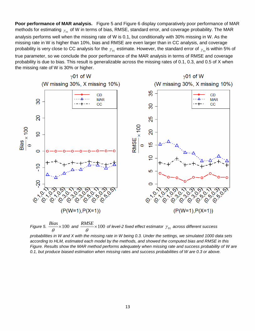
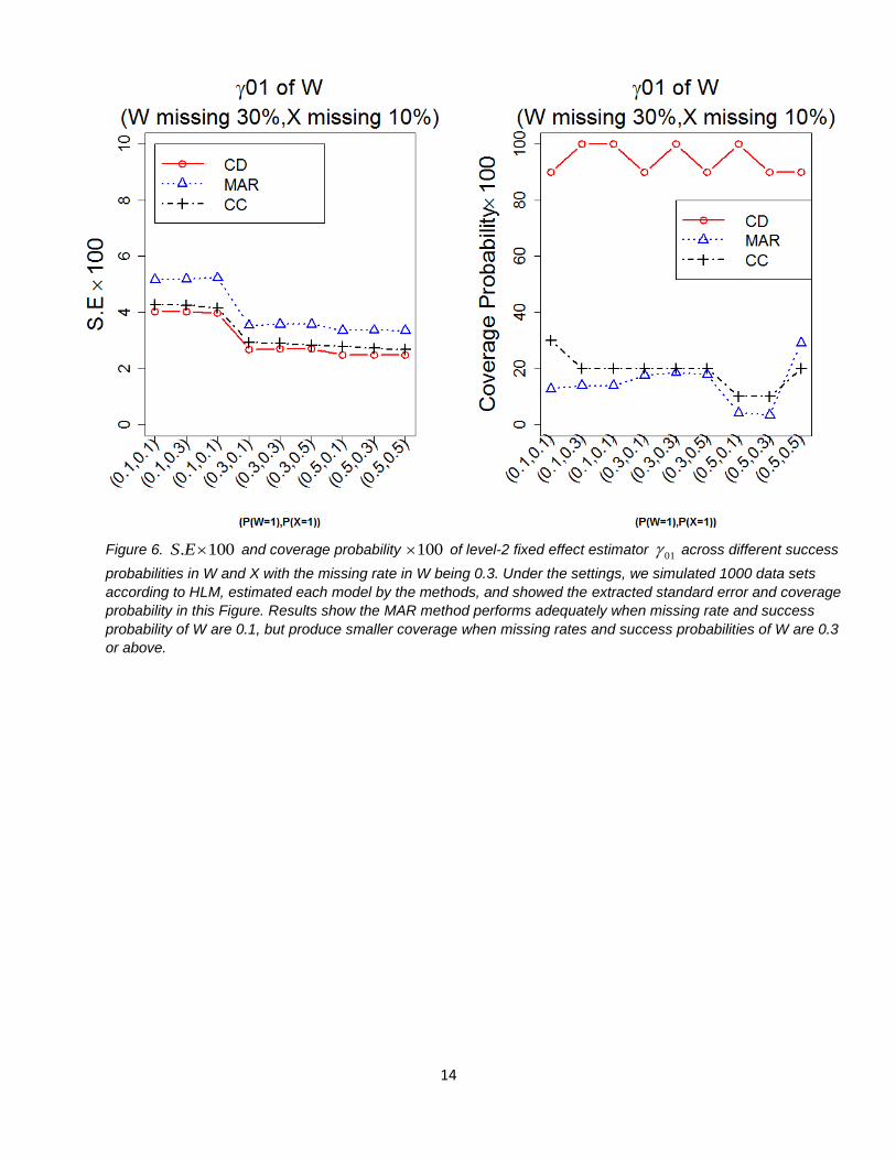
Poor performance of MAR analysis. Figure 5 and Figure 6 display comparatively poor performance of MAR
methods for estimating 01 of W in terms of bias, RMSE, standard error, and coverage probability. The MAR
analysis performs well when the missing rate of W is 0.1, but conditionally with 30% missing in W. As the
missing rate in W is higher than 10%, bias and RMSE are even larger than in CC analysis, and coverage
probability is very close to CC analysis for the 01 estimate. However, the standard error of
01 is within 5% of
true parameter, so we conclude the poor performance of the MAR analysis in terms of RMSE and coverage
probability is due to bias. This result is generalizable across the missing rates of 0.1, 0.3, and 0.5 of X when
the missing rate of W is 30% or higher.
Figure 5. 100Bias
and 100
RMSE
of level-2 fixed effect estimator
01 across different success
probabilities in W and X with the missing rate in W being 0.3. Under the settings, we simulated 1000 data sets
according to HLM, estimated each model by the methods, and showed the computed bias and RMSE in this
Figure. Results show the MAR method performs adequately when missing rate and success probability of W are
0.1, but produce biased estimation when missing rates and success probabilities of W are 0.3 or above.
14
Figure 6. . 100S E and coverage probability 100 of level-2 fixed effect estimator 01 across different success
probabilities in W and X with the missing rate in W being 0.3. Under the settings, we simulated 1000 data sets
according to HLM, estimated each model by the methods, and showed the extracted standard error and coverage
probability in this Figure. Results show the MAR method performs adequately when missing rate and success
probability of W are 0.1, but produce smaller coverage when missing rates and success probabilities of W are 0.3
or above.

15
Figure 7 and Figure 8 display comparatively poor performance of MAR method for estimating in terms of
bias, RMSE, standard error, and coverage probability. For estimating , the MAR analysis only performs well
when the missing rate or success probability of W are 0.1, but performs comparatively poorly for missing rates
and success probabilities of W greater than 0.1. As the missing rate of W increases, bias and RMSE get
comparatively larger, and coverage probability gets even smaller than CC analysis. However, the standard
error of is with 5% of true parameter values. The poor performance of the MAR analysis is generalizable
across the missing rates of 0.1, 0.3, and 0.5 of X.
Figure 7. 100Bias
and 100
RMSE
of level-2 random effect estimator across different success
probabilities in W and X with the missing rate in W being 0.1 or 0.3. Results show the MAR method performs fine
when missing rate and success probability of W are 0.1, but produces biased estimation when missing rates or
success probabilities of W are 0.3 or above.
16
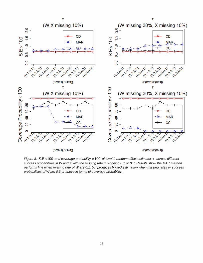
Figure 8. . 100S E and coverage probability 100 of level-2 random effect estimator across different
success probabilities in W and X with the missing rate in W being 0.1 or 0.3. Results show the MAR method
performs fine when missing rate of W are 0.1, but produces biased estimation when missing rates or success
probabilities of W are 0.3 or above in terms of coverage probability.

17
Unexplained performance of MAR analysis for future investigation. Bias of level-1 random effect 2
shows bumps when the success probabilities of W and X are (0.1, 0.5) and (0.3, 0.5). As probability and
missing rate of W increase, the bumps tend to be comparatively higher (Figure 5). Thus, bias gets larger when
the success probability and missing rate of W increase. This phenomenon needs further investigation. We can
vary the missing rate and success probability in a model having X or W only for comparison to determine what
factors contribute to this phenomenon.
Figure 9. 100Bias
of level-1 variance
2 across different success probabilities of W and X with the missing
rate of W being 0.1, 0.3, and 0.5. Results show bias bumps when success probabilities of W and X are (0.1,0.5)
and (0.3,0.5).

18
4.2 Second Experiment.
This section explains the performance of MAR analysis with binary missing data in terms of bias, RMSE,
standard error, and coverage probability. We make the missing pattern depending on completely observed
continuous third covariate Z in single X, single W, and combined X and W models. We first give an overall
summary of results based on the three methods. Second, we illustrate the performance of MAR analysis and
state cases where researchers should be careful about using the MAR analysis and list out the cases when
MAR analysis performs well. We provide detailed outputs and codes in the Appendices. The bias and RMSE of
CC analysis are very close to the CD analysis, the benchmark analysis, when the missing pattern depends on
completely observed covariate Z in the three models. However, CC analysis produces larger standard error
than MAR analysis.
With missing values of binary covariates, the MAR estimation produces unbiased estimators of fixed effects
and variances when W has 10% missing rate. This is consistent with our first experiment when the missing
pattern depends on continuous response variable Y.
19
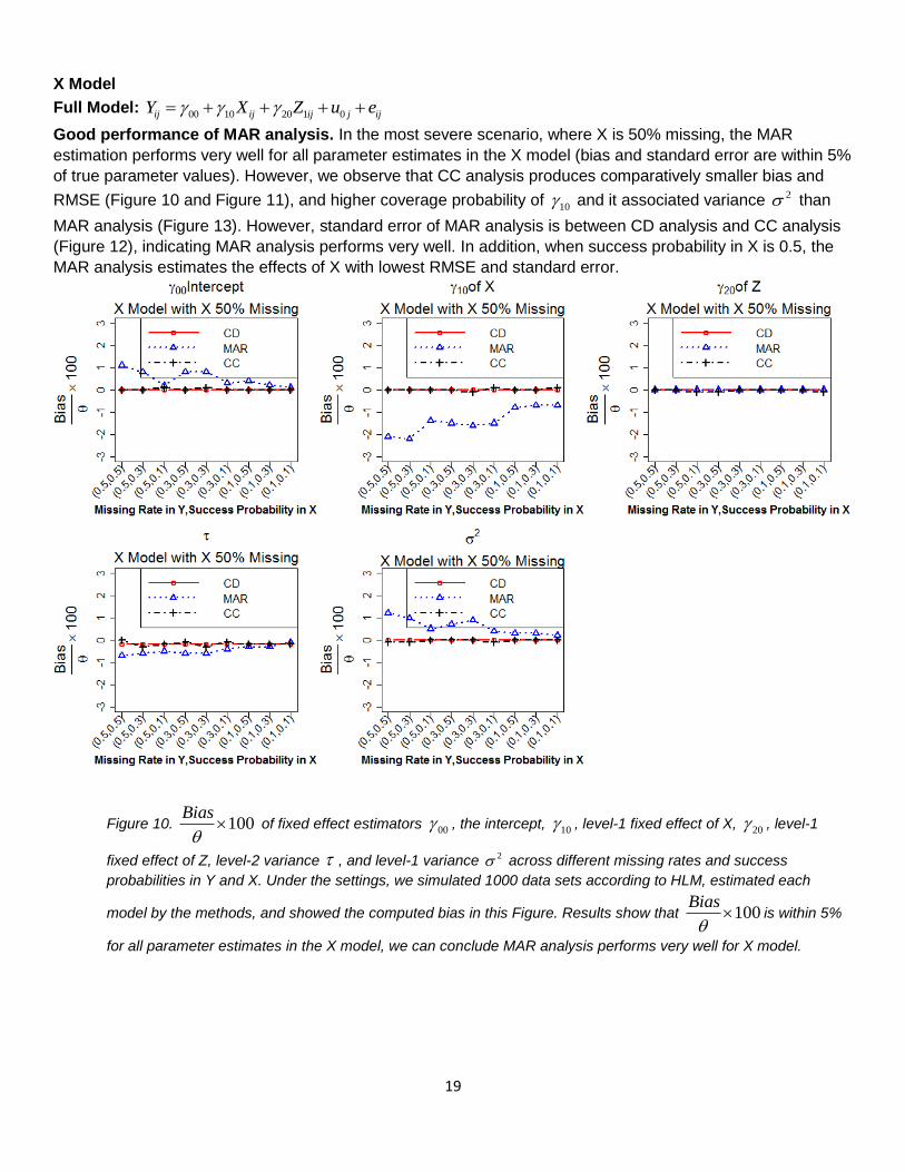
X Model
Full Model: 00 10 20 1 0ij ij ij j ijY X Z u e
Good performance of MAR analysis. In the most severe scenario, where X is 50% missing, the MAR
estimation performs very well for all parameter estimates in the X model (bias and standard error are within 5%
of true parameter values). However, we observe that CC analysis produces comparatively smaller bias and
RMSE (Figure 10 and Figure 11), and higher coverage probability of 10 and it associated variance 2 than
MAR analysis (Figure 13). However, standard error of MAR analysis is between CD analysis and CC analysis
(Figure 12), indicating MAR analysis performs very well. In addition, when success probability in X is 0.5, the
MAR analysis estimates the effects of X with lowest RMSE and standard error.
Figure 10. 100Bias
of fixed effect estimators 00 , the intercept, 10 , level-1 fixed effect of X, 20 , level-1
fixed effect of Z, level-2 variance , and level-1 variance 2 across different missing rates and success
probabilities in Y and X. Under the settings, we simulated 1000 data sets according to HLM, estimated each
model by the methods, and showed the computed bias in this Figure. Results show that 100Bias
is within 5%
for all parameter estimates in the X model, we can conclude MAR analysis performs very well for X model.

20
Figure 11. 100RMSE
of fixed effect estimators 00 , the intercept, 10 , level-1 fixed effect of X, 20 , level-1
fixed effect of Z, level-2 variance , and level-1 variance 2 across different missing rates and success
probabilities in Y and X. We use the estimated parameters in Figure 1 to draw 100RMSE
. Results show that
100RMSE
is within 10% for all parameter estimates in X model, we can conclude MAR analysis performs very
well for X model.
21
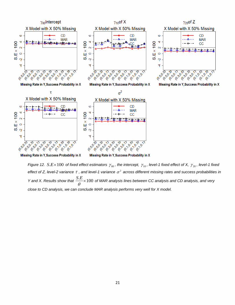
Figure 12. . 100S E of fixed effect estimators 00 , the intercept, 10 , level-1 fixed effect of X, 20 , level-1 fixed
effect of Z, level-2 variance , and level-1 variance 2 across different missing rates and success probabilities in
Y and X. Results show that .
100S E
of MAR analysis lines between CC analysis and CD analysis, and very
close to CD analysis, we can conclude MAR analysis performs very well for X model.

22
Figure 13. Coverage probability 100 of fixed effect estimators 00 , the intercept,
10 , level-1 fixed effect of X,
20 , level-1 fixed effect of Z, level-2 variance , and level-1 variance 2 across different missing rates and
success probabilities in Y and X. Results show that coverage probability of all parameter estimators are very
close to CD analysis except for 10 of X and its associated variance has comparatively smaller coverage
probability.

23
W Model
Full Model: 00 01 02 2 0ij j j j ijY W Z u e
Good performance of MAR analysis. In the most severe scenario, when W is 50% missing, the MAR
estimation performs very well for 02 , fixed effect of level-2 completely observed continuous covariate
2Z and
level-1 variance 2 across different missing rates in Y and success probabilities in W (Bias and RMSE are
within 5% of true parameter value).
Figure 14. 100Bias
and 100
RMSE
of 02 , fixed effect of level-2 completely observed continuous
covariate 2Z and level-1variance 2 across different missing rates in Y and success probabilities in W when W is
50% missing. Under the settings, we simulated 1000 data sets according to HLM, estimated each model by the
methods, and showed the computed bias and RMSE in this Figure. Results show that 100Bias
and
100RMSE
are within 5% of the true parameter values, indicating the MAR analysis performances well for 02
and 2 .

24
Poor performance of MAR analysis. Table 7A and Table 8A, sub portions of Table 7 and Table 8, as well as
Figure 15 represent the poor performance of the MAR method of parameter estimates 00 , the intercept, fixed
effect of level-2 binary covariate, 01 , and level-2 random effect in terms of bias and RMSE. We observed
that 01 , parameter estimate of level-2 covariate W, is highly biased when the missing rate of W is 0.3 and
above regardless of the missing rate of Y. However, the MAR method performs fine when success probability
of W is 0.1 for 01 , the intercept, and level-2 random effect when the missing rate of W is 0.3. Figure 16
represents the performance of MAR analysis in terms of standard error and coverage probability, the coverage
probability shows the same poor performance of the MAR method as bias and RMSE. However, the standard
errors of 00 and are within 10% of true parameter values, thus the poor performance results of RMSE and
coverage probability are due to bias.
Table 7A. 100Bias
of
00 , the intercept, fixed effect of level-2 binary covariate, 01 , and level-2 random effect
across 18 different combinations of missing rates of W and Y, and success probabilities of W
00
01
MW MY PW CD MAR CC CD MAR CC CD MAR CC
0.5 0.5 0.5 -0.1 24.4 -0.2 0.3 -39.8 0.2 -0.3 16.3 -0.2
0.3 -0.1 17.6 -0.3 0.2 -40.2 0.8 -0.3 15.2 -0.4
0.1 -0.1 7.9 -0.2 0.4 -42.6 -0.6 -0.3 8.4 -0.6
0.3 0.5 -0.1 25.2 -0.1 0.3 -41.4 0.3 -0.3 16.8 -0.4
0.3 -0.1 18.2 -0.2 0.2 -42.2 0.4 -0.3 16.0 -0.5
0.1 -0.1 8.0 -0.1 0.4 -44.0 0.1 -0.3 8.7 -0.7
0.1 0.5 -0.1 25.6 -0.4 0.3 -42.4 0.3 -0.3 17.4 -0.3
0.3 -0.1 18.6 0.0 0.2 -43.4 -0.2 -0.3 16.3 -0.2
0.1 -0.1 8.3 0.1 0.4 -46.1 -0.7 -0.3 8.8 -0.5
0.3 0.5 0.5 -0.1 16.5 -0.1 0.3 -25.2 0.0 -0.3 11.5 -0.3
0.3 -0.1 12.3 -0.3 0.2 -25.6 0.4 -0.3 11.3 -0.2
0.1 -0.1 5.9 0.0 0.4 -28.2 -0.4 -0.3 6.4 -0.7
0.3 0.5 -0.1 17.2 -0.2 0.3 -26.7 -0.1 -0.3 12.0 -0.6
0.3 -0.1 12.5 0.1 0.2 -26.5 -0.2 -0.3 11.6 -0.3
0.1 -0.1 5.8 0.0 0.4 -28.8 0.2 -0.3 6.6 -0.3
0.1 0.5 -0.1 17.4 0.1 0.3 -27.2 -0.3 -0.3 12.3 -0.5
0.3 -0.1 12.9 0.0 0.2 -27.8 0.2 -0.3 11.9 -0.3
0.1 -0.1 6.0 -0.1 0.4 -29.9 0.2 -0.3 6.8 -0.3
MW: Missing rate of W
MY: Missing rate of Y
PW: Success probability of W

25
Table 8A. 100RMSE
of
00 , the intercept, fixed effect of level-2 binary covariate, 01 , and level-2 random
effect across 18 different combinations of missing rates of W and Y, and success probabilities of W
00
01
MW MY PW CD MAR CC CD MAR CC CD MAR CC
0.5 0.5 0.5 4.5 25.0 6.2 6.5 40.6 9.3 4.6 17.3 7.2
0.3 3.9 18.3 5.6 6.9 41.1 10.7 4.6 16.3 7.1
0.1 3.5 8.9 5.1 10.0 44.2 16.4 4.6 10.2 7.0
0.3 0.5 4.5 25.7 6.2 6.5 42.1 9.2 4.6 17.8 7.1
0.3 3.9 18.8 5.5 6.9 43.1 10.6 4.6 17.0 6.6
0.1 3.5 8.9 4.7 10.0 45.4 16.1 4.6 10.2 6.9
0.1 0.5 4.5 26.2 6.2 6.5 43.1 9.2 4.6 18.2 6.8
0.3 3.9 19.2 5.4 6.9 44.2 10.5 4.6 17.3 6.8
0.1 3.5 9.1 5.0 10.0 47.3 15.9 4.6 10.3 6.6
0.3 0.5 0.5 4.5 17.3 5.8 6.5 26.5 8.7 4.6 12.9 6.2
0.3 3.9 13.2 5.0 6.9 26.9 9.2 4.6 12.7 6.2
0.1 3.5 7.0 4.3 10.0 30.4 13.8 4.6 8.5 6.2
0.3 0.5 4.5 18.0 5.3 6.5 27.7 8.3 4.6 13.2 5.8
0.3 3.9 13.2 4.9 6.9 27.7 9.2 4.6 12.8 5.9
0.1 3.5 6.9 4.3 10.0 30.7 13.1 4.6 8.4 5.9
0.1 0.5 4.5 18.2 5.3 6.5 28.2 8.1 4.6 13.4 5.7
0.3 3.9 13.7 4.6 6.9 29.0 8.5 4.6 13.0 5.6
0.1 3.5 7.0 4.0 10.0 31.8 12.6 4.6 8.4 5.7
MW: Missing rate of W
MY: Missing rate of Y
PW: Success probability of W
26
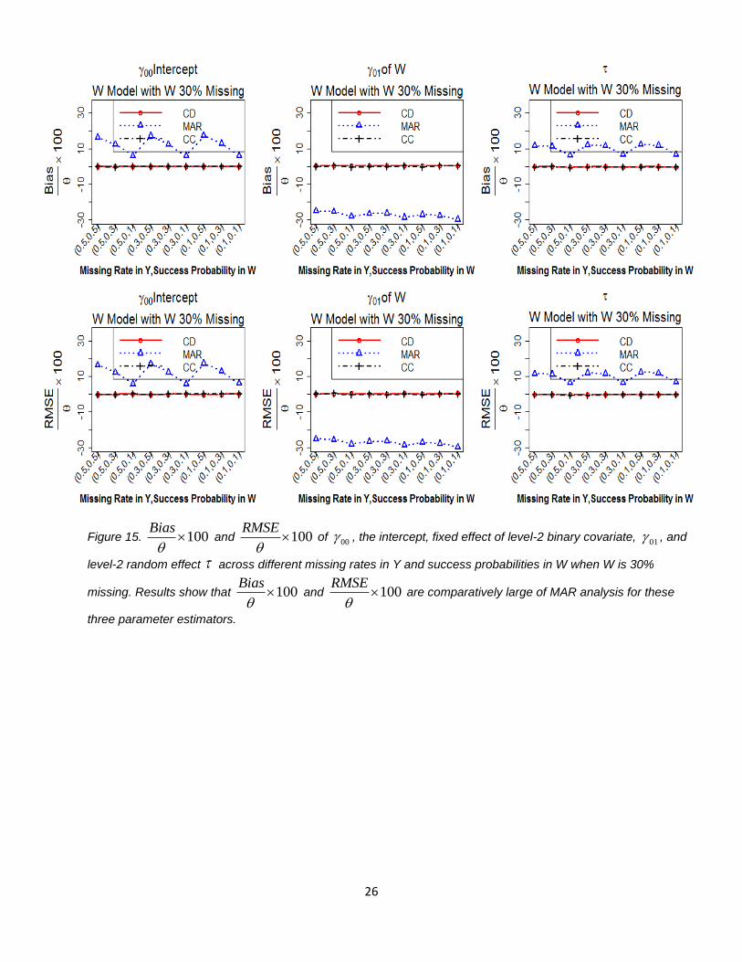
Figure 15. 100Bias
and 100
RMSE
of 00 , the intercept, fixed effect of level-2 binary covariate, 01 , and
level-2 random effect across different missing rates in Y and success probabilities in W when W is 30%
missing. Results show that 100Bias
and 100
RMSE
are comparatively large of MAR analysis for these
three parameter estimators.

27
Figure 16. . 100S E and coverage probability 100 of 00 , the intercept, fixed effect of level-2 binary covariate,
01 , and level-2 random effect across different missing rates in Y and success probabilities in. Results show
that standard error of 00 and is within 10% of true parameter values when W is 50% missing. Standard errors
of 00 and are within 10% of true parameter values.
28
X and W Model
Full Model: 00 01 02 2 10 20 1 0ij j j ij ij j ijY W Z X Z u e
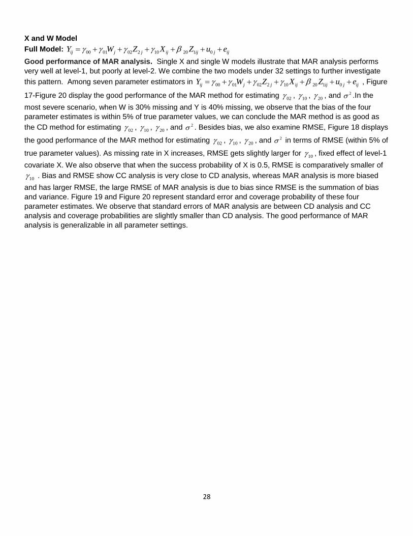
Good performance of MAR analysis. Single X and single W models illustrate that MAR analysis performs
very well at level-1, but poorly at level-2. We combine the two models under 32 settings to further investigate
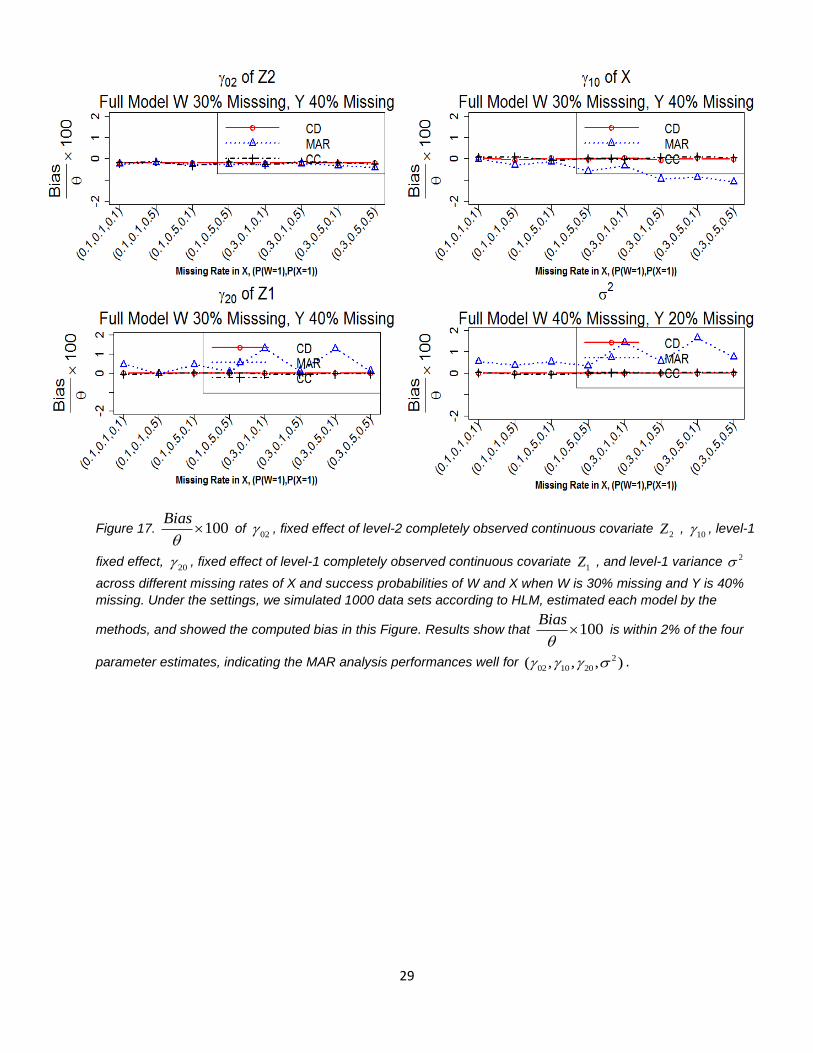
this pattern. Among seven parameter estimators in 00 01 02 2 10 20 1 0ij j j ij ij j ijY W Z X Z u e , Figure
17-Figure 20 display the good performance of the MAR method for estimating 02 ,
10 , 20 , and 2 .In the
most severe scenario, when W is 30% missing and Y is 40% missing, we observe that the bias of the four
parameter estimates is within 5% of true parameter values, we can conclude the MAR method is as good as
the CD method for estimating 02 ,
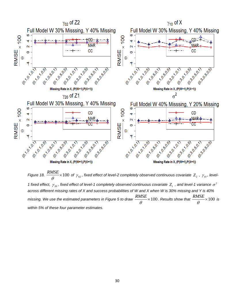
10 , 20 , and 2 . Besides bias, we also examine RMSE, Figure 18 displays
the good performance of the MAR method for estimating 02 ,
10 , 20 , and 2 in terms of RMSE (within 5% of
true parameter values). As missing rate in X increases, RMSE gets slightly larger for 10 , fixed effect of level-1
covariate X. We also observe that when the success probability of X is 0.5, RMSE is comparatively smaller of
10 . Bias and RMSE show CC analysis is very close to CD analysis, whereas MAR analysis is more biased
and has larger RMSE, the large RMSE of MAR analysis is due to bias since RMSE is the summation of bias
and variance. Figure 19 and Figure 20 represent standard error and coverage probability of these four
parameter estimates. We observe that standard errors of MAR analysis are between CD analysis and CC
analysis and coverage probabilities are slightly smaller than CD analysis. The good performance of MAR
analysis is generalizable in all parameter settings.
29
Figure 17. 100Bias
of
02 , fixed effect of level-2 completely observed continuous covariate 2Z ,
10 , level-1
fixed effect, 20 , fixed effect of level-1 completely observed continuous covariate
1Z , and level-1 variance 2
across different missing rates of X and success probabilities of W and X when W is 30% missing and Y is 40%
missing. Under the settings, we simulated 1000 data sets according to HLM, estimated each model by the
methods, and showed the computed bias in this Figure. Results show that 100Bias
is within 2% of the four
parameter estimates, indicating the MAR analysis performances well for 2
02 10 20( , , , ) .
30
Figure 18. 100RMSE
of
02 , fixed effect of level-2 completely observed continuous covariate 2Z ,
10 , level-
1 fixed effect, 20 , fixed effect of level-1 completely observed continuous covariate
1Z , and level-1 variance 2
across different missing rates of X and success probabilities of W and X when W is 30% missing and Y is 40%
missing. We use the estimated parameters in Figure 5 to draw 100RMSE
. Results show that 100
RMSE
is
within 5% of these four parameter estimates.

31
Figure 19. . 100S E of 02 , fixed effect of level-2 completely observed continuous covariate
2Z , 10 , level-1
fixed effect, 20 , fixed effect of level-1 completely observed continuous covariate
1Z , and level-1 variance 2
across different missing rates of X and success probabilities of W and X when W is 30% missing and Y is 40%
missing. Results show that . 100S E is within 5% of these four parameter estimates.

32
Figure 20. Coverage probability 100 of
02 , fixed effect of level-2 completely observed continuous covariate
2Z , 10 , level-1 fixed effect,
20 , fixed effect of level-1 completely observed continuous covariate 1Z , and level-
1 variance 2 across different missing rates of X and success probabilities of W and X when W is 30% missing
and Y is 40% missing. Results show that coverage probabilities of MAR analysis are slightly smaller than CD
analysis.

33
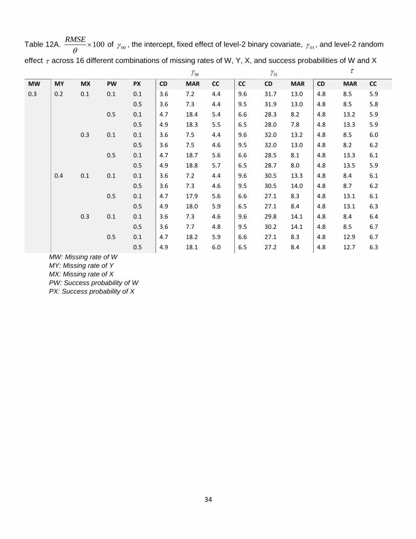
Poor performance of MAR analysis. Table 11A and Table 12A, sub portions of Table 11 and Table 12, as
well as Figure 21 represent the poor performance of the MAR method for parameter estimates 00 , the
intercept, fixed effect of level-2 binary covariate, 01 , and level-2 random effect in terms of bias and RMSE.
We observe that 01 , parameter estimate of level-2 covariate W, is highly biased when missing rate of W is 0.3
and missing rate of Y is 0.2 and above. This is consistent with our previous studies. However, the MAR method
performs fine when success probability of W is 0.1 for intercept 00 and level-2 variance when missing rate
of W is 0.3. When missing rates of Y and X increase, bias and RMSE only increase slightly, indicating
missingness in Y or X does not undermine the performance of the MAR method. This result is consistent with
the result from coverage probability pattern for the combined model (Figure 23). The poor performance of the
MAR analysis is generalizable in all parameter settings in terms of bias, RMSE, and coverage probability.
Figure 22 shows the standard error of 00 ,
01 , and , we observe that in most severe scenario, when W is
30% missing and Y is 40% missing, MAR analysis performs tolerable for parameter estimates 00 , the
intercept and level-2 random effect , and fixed effect of level-2 binary covariate, 01 , when success
probability of W is 0.5. The large RMSE and low coverage probability is due to bias, thus we look at standard
error to obtain more useful information.
Table 11A. 100Bias
of
00 , the intercept, fixed effect of level-2 binary covariate, 01 , and level-2 random
effect across 16 different combinations of missing rates of W, Y, X, and success probabilities of W and X
00 01
MW MY MX PW PX CD MAR CC CD MAR CC CD MAR CC
0.3 0.2 0.1 0.1 0.1 0.0 6.1 0.2 0.2 -29.9 -0.5 -0.4 6.6 -0.5
0.5 0.0 6.2 0.0 0.0 -30.1 0.3 -0.4 6.6 -0.6
0.5 0.1 0.2 17.7 0.0 -0.4 -27.3 0.0 -0.4 12.1 -0.5
0.5 0.0 17.5 0.2 -0.1 -27.0 -0.4 -0.4 12.2 -0.4
0.3 0.1 0.1 0.0 6.5 0.0 0.2 -30.0 0.5 -0.4 6.6 -0.7
0.5 0.0 6.4 0.1 0.0 -30.1 0.0 -0.4 6.4 -0.6
0.5 0.1 0.2 18.0 0.0 -0.4 -27.5 0.1 -0.4 12.1 -0.3
0.5 0.0 17.9 0.0 -0.1 -27.5 0.0 -0.4 12.0 -0.7
0.4 0.1 0.1 0.1 0.0 6.0 0.1 0.2 -28.3 -0.6 -0.4 6.4 -1.0
0.5 0.0 6.0 0.0 0.0 -28.5 -0.5 -0.4 6.7 -0.7
0.5 0.1 0.2 17.1 0.2 -0.4 -26.0 -0.4 -0.4 11.8 -0.5
0.5 0.0 17.1 0.0 -0.1 -26.0 0.1 -0.4 11.8 -0.7
0.3 0.1 0.1 0.0 6.2 0.0 0.2 -27.7 -0.4 -0.4 6.4 -0.6
0.5 0.0 6.3 -0.2 0.0 -28.1 0.4 -0.4 6.3 -0.8
0.5 0.1 0.2 17.4 -0.2 -0.4 -26.0 0.1 -0.4 11.6 -0.6
0.5 0.0 17.4 0.2 -0.1 -26.2 -0.2 -0.4 11.5 -0.6
MW: Missing rate of W
MY: Missing rate of Y
MX: Missing rate of X
PW: Success probability of W
PX: Success probability of X
34
Table 12A. 100RMSE
of
00 , the intercept, fixed effect of level-2 binary covariate, 01 , and level-2 random
effect across 16 different combinations of missing rates of W, Y, X, and success probabilities of W and X
00
01
MW MY MX PW PX CD MAR CC CC CD MAR CD MAR CC
0.3 0.2 0.1 0.1 0.1 3.6 7.2 4.4 9.6 31.7 13.0 4.8 8.5 5.9
0.5 3.6 7.3 4.4 9.5 31.9 13.0 4.8 8.5 5.8
0.5 0.1 4.7 18.4 5.4 6.6 28.3 8.2 4.8 13.2 5.9
0.5 4.9 18.3 5.5 6.5 28.0 7.8 4.8 13.3 5.9
0.3 0.1 0.1 3.6 7.5 4.4 9.6 32.0 13.2 4.8 8.5 6.0
0.5 3.6 7.5 4.6 9.5 32.0 13.0 4.8 8.2 6.2
0.5 0.1 4.7 18.7 5.6 6.6 28.5 8.1 4.8 13.3 6.1
0.5 4.9 18.8 5.7 6.5 28.7 8.0 4.8 13.5 5.9
0.4 0.1 0.1 0.1 3.6 7.2 4.4 9.6 30.5 13.3 4.8 8.4 6.1
0.5 3.6 7.3 4.6 9.5 30.5 14.0 4.8 8.7 6.2
0.5 0.1 4.7 17.9 5.6 6.6 27.1 8.3 4.8 13.1 6.1
0.5 4.9 18.0 5.9 6.5 27.1 8.4 4.8 13.1 6.3
0.3 0.1 0.1 3.6 7.3 4.6 9.6 29.8 14.1 4.8 8.4 6.4
0.5 3.6 7.7 4.8 9.5 30.2 14.1 4.8 8.5 6.7
0.5 0.1 4.7 18.2 5.9 6.6 27.1 8.3 4.8 12.9 6.7
0.5 4.9 18.1 6.0 6.5 27.2 8.4 4.8 12.7 6.3
MW: Missing rate of W
MY: Missing rate of Y
MX: Missing rate of X
PW: Success probability of W
PX: Success probability of X
35
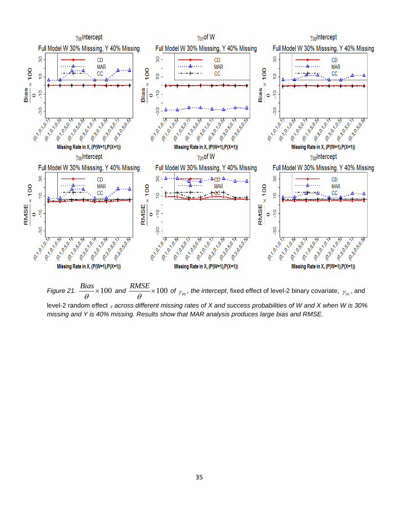
Figure 21. 100Bias
and 100
RMSE
of
00 , the intercept, fixed effect of level-2 binary covariate, 01 , and
level-2 random effect across different missing rates of X and success probabilities of W and X when W is 30%
missing and Y is 40% missing. Results show that MAR analysis produces large bias and RMSE.
36
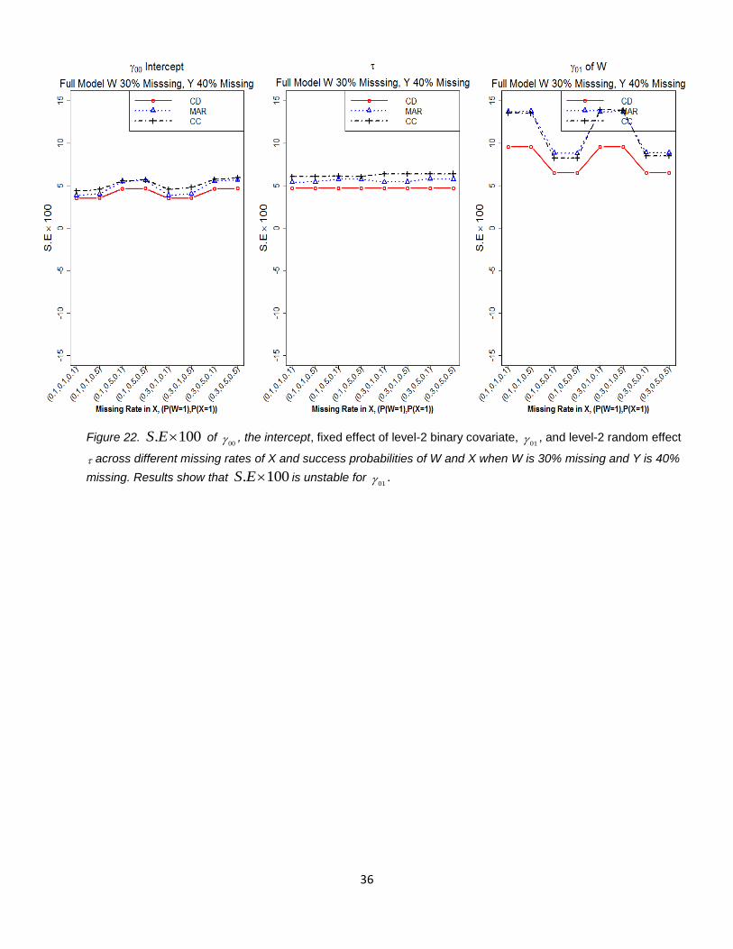
Figure 22. . 100S E of 00 , the intercept, fixed effect of level-2 binary covariate,
01 , and level-2 random effect
across different missing rates of X and success probabilities of W and X when W is 30% missing and Y is 40%
missing. Results show that . 100S E is unstable for 01 .
37
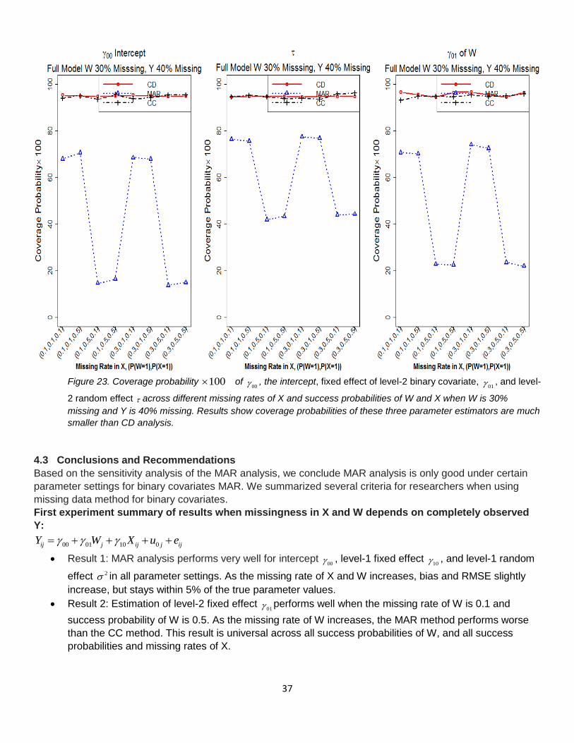
Figure 23. Coverage probability 100 of
00 , the intercept, fixed effect of level-2 binary covariate, 01 , and level-
2 random effect across different missing rates of X and success probabilities of W and X when W is 30%
missing and Y is 40% missing. Results show coverage probabilities of these three parameter estimators are much
smaller than CD analysis.
4.3 Conclusions and Recommendations
Based on the sensitivity analysis of the MAR analysis, we conclude MAR analysis is only good under certain
parameter settings for binary covariates MAR. We summarized several criteria for researchers when using
missing data method for binary covariates.
First experiment summary of results when missingness in X and W depends on completely observed
Y:
00 01 10 0ij j ij j ijY W X u e
Result 1: MAR analysis performs very well for intercept 00 , level-1 fixed effect
10 , and level-1 random
effect 2 in all parameter settings. As the missing rate of X and W increases, bias and RMSE slightly
increase, but stays within 5% of the true parameter values.
Result 2: Estimation of level-2 fixed effect 01 performs well when the missing rate of W is 0.1 and
success probability of W is 0.5. As the missing rate of W increases, the MAR method performs worse
than the CC method. This result is universal across all success probabilities of W, and all success
probabilities and missing rates of X.

38
Result 3: The MAR estimation of level-2 variance is good only when the missing rate and success
probability of W are 0.1, regardless of the success probabilities and missing rates of X. As the missing
rate of W increases, the MAR method performs worse than the CC method.
Second experiment summary of results when missingness in X or W or Y depends on Z:
Result 1: MAR analysis performs very well for all parameter estimates. Estimation of level-1 fixed effect
10 is very good when the success probability of X is 0.5 for the X model.
Result 2: MAR performs very well for 02 , fixed effect of level-2 completely observed continuous
covariate 2Z and level-1variance 2 across different missing rates of Y and W, and success
probabilities of W for the W model. Estimation of intercept 00 and level-2 variance is good only when
the missing rate and success probability of W are 0.1. Estimation of level-2 fixed effect 01 performs well
when the missing rate of W is 0.1 and success probability of W is 0.5.
Result 3: Results from the full model are consistent with the results from single X and single W model.
MAR analysis performs very well for fixed effect 10 of level-1 binary covariate, fixed
20 of level-1
continuous covariate, level-1 random effect 2 , fixed effect 02 of level-2 binary covariate across
different missing rates of Y and W, and success probabilities of W and X for the combined X and W
model. Estimations of intercept 00 and level-2 variance are good only when the missing rate and
success probability of W are 0.1. Estimation of level-2 fixed effect 01 performs well when the missing
rate of W is 0.1 and success probability of W is 0.5.
Based on the results, we summarized cases when MAR analysis performs fine
W Y X
MISSING RATE 0.1 0.2, 0.4 0.1, 0.3
SUCCESS PROBABILITY
0.5 0.5
Multilevel data can be missing at different levels. The usual solution to handle data missing in multilevel model
is to remove any incomplete records, which is wasteful and could bias the estimates of interest. The efficient
MAR analysis rexpresses the desired model as a joint distribution of variables that are subject to missingness
conditional on all of the covariates that are completely observed, and estimate the joint model by full ML;
generate multiple imputation given the ML estimates of the joint distribution; analyze the desired hierarchical
model by complete data analysis given the multiple imputation; and then combine the multiple hierarchical
model estimates [10]. However, with discrete covariates, the missing data analysis is robust under certain
parameter settings. Efficient analysis performs very well for estimation of02 ,
10 ,20 , and 2 across varying
success probabilities of W and X and missing rates of Y, W, and X. Researchers should be careful when using
the MAR method for estimating 00 ,
01 , and because the estimation is good only when missing rate of W is
0.1.
4.4 Synthesizing the Results
When missing patterns depend on completely observed response variable Y, we obtain large bias and RMSE
for CC analysis because Y contains random effects and 2 ; however, CC analysis is very close to CD
analysis when missing pattern depends on covariate Z in the model. This is could due to we simulate Z
independently that MAR assumption might be violated, thus we look at standard error and coverage probability
of each parameter estimator, results show standard error for CC analysis is larger than MAR analysis,

39
indicating CC analysis is never a reasonable method. Based on the two experiments, we can conclude the
MAR method is not well suitable for level 2 binary covariate. More studies could be done to investigate this
phenomenon.
4.5 Limitations and Future Work
The first experiment simulates missingness in X and W depending on the completely observed response
variable Y. However, response variable Y is typically subject to missingness in reality. In order to generalize
the results, we make the missing pattern depend on covariate Z that are completely observed under the MAR
assumption in the second experiment. In the future, we can further investigate Z model by excluding Z in the
model. From our first experiment, the MAR estimation of 2 is not stable, in particular, when success
probabilities in W and X are (0.1, 0.5) and (0.3, 0.5), and this pattern needs further investigation. We
investigate this pattern by an extended simulation study of an HLM given either X or W only in our second
experiment. Cross-comparing the results will tell us at least partly why the poor estimation of the variance
occurs. However, since our missing pattern setting is different, the second experiment does not explain this
pattern. We can extend our first experiment given X or W only with same missing pattern setting. In addition to
the binary covariates in HLM2, we will expand our sensitivity analysis to ordinal and nominal covariates MAR.
Section 5 Data application We use National Growth and Health Study (NGHS) data for missing data analysis. The National Heart, Lung,
and Blood Institute initiated NGHS to investigate racial differences in dietary, physical activity, family, and
psychosocial factors associated with the development of obesity from pre-adolescence through maturation of
African-American and white girls. It collected data on development of obesity and factors associated with the
development from 1,213 African-American and 1,166 white girls. The study followed the subjects from 1987-
1988 when they were 9 to 10 years old until 1996-1997 when they were 18 to 19 years old [21].
The subjects were assessed on development of obesity and related factors annually.
The goal of this study is to identify the risk factors for obesity. This study is a longitudinal where level-1
variables are time-varying while level-2 variables are individual-level or base-line characteristics, and missing
data are present at both levels under the assumption of data missing at random.
Based on Table 15, possible biomarkers for obesity are maximum below-waist circumference (MAXBLOAV), sum of skinfolds at triceps, subscapular, and suprailiac sites (SUMSKIN), and body mass index (BMI). Sum of skinfolds measurement is a commonly used method to determine body fat percentage by skinfold thickness. Obesity is defined (SUMSKIN> 150+mm) for a normal female. Possible level-1 covariates are TV watching in hours per week; continuous with mean of 31 hours, maturation stage; the emergence of individual and behavioral characteristics through growth processes over time; ordinal coded into 4 classes. Possible level-2 covariates are Mother’s BMI; the ratio of body weight in kilograms and height in meters squared, is widely used
to define obesity (BMI 30), race (white/black), smoke; whether parent is a current smoker, and relation of mother/female guardian(natural/adopted). To make variable setting close to good cases of MAR analysis, we choose SUMSKIN as an outcome variable to identify risk factors of child obesity, categorize TV watching (hours/week) at level-1 into binary with success probability 0.5 (1 if TV watching hours/week>31, 0 otherwise), categorize Household Income (Income) at level-2 into binary with success probability 0.5 (1 if income 0-40K, 0 otherwise).

40
Variable selection for analysis W Y X
Income SUMSKIN TV
MISSING RATE 5.5 3.8 23.2
SUCCESS PROBABILITY
0.5 0.5
Table 15. Descriptive statistics of NHGS
VARIABLE LABEL MEAN STD
DEV
N
MISS
MISS
%
LEVEL 1 MAXBLOAV Max below waist circumference
(cm)
93.9 12.9 2811 13.5
SUMSKIN Sum of skinfolds (mm) 45.1 24.9 785 3.8
BMI Body Mass Index (Kg/m2) 22.4 5.8 309 1.5
TV 1 if TV watching hours/week>31, 0
otherwise
0.5 0.5 4841 23.2
MATSTAGE Maturation stage (4 classes) 3.1 1.0 1066 5.1
AGE Age at Time of Exam 14.4 3.0 0 0.0
LEVEL 2 M_BMI Mother BMI (Kg/m2) 27.7 6.9 6320 30.3
TRICAV Mother Average Triceps Skinfold 23.6 9.7 6178 29.6
Income 1 if household income 0-40K, 0
otherwise 0.6 0.5 1157 5.5
CATEDUC Max parental education (grouped) 2.1 0.8 15 0.1
RACE Race (White/Black) 1.5 0.5 0 0.0
SMOKE5 smoke >5 past year 2.0 0.1 9894 47.4
SMOKE Current smoker 2.0 0.2 12219 58.5
MSAMHOUS Father living in same house 1.0 0.1 15631 74.8
FSAMHOUS Mother living in same house 1.0 0.0 5828 27.9
FRELAT Relation of mother/female guardian 1.1 0.4 293 1.4
Based on our simulation study, the missing patterns of level-1 and level-2 binary covariates depend on third
covariate Z in the model, thus in the examining NHGS data, we first need to determine what Z variables are in
the model that predict missing patterns of level-1 and level-2 binary covariates TV and Income.
Missing pattern model of level-1 binary covariate X (TV Watching per Week)
0 1 11 2 12 1
0 1 2 3 4
log (P(Mx 1) ...ij p p xj
j j ij ij xj
it Z Z Z u
MotherBMI Race Age MATSTAGE u
Mxij : Missing pattern of X (1 missing; 0 not missing)
41
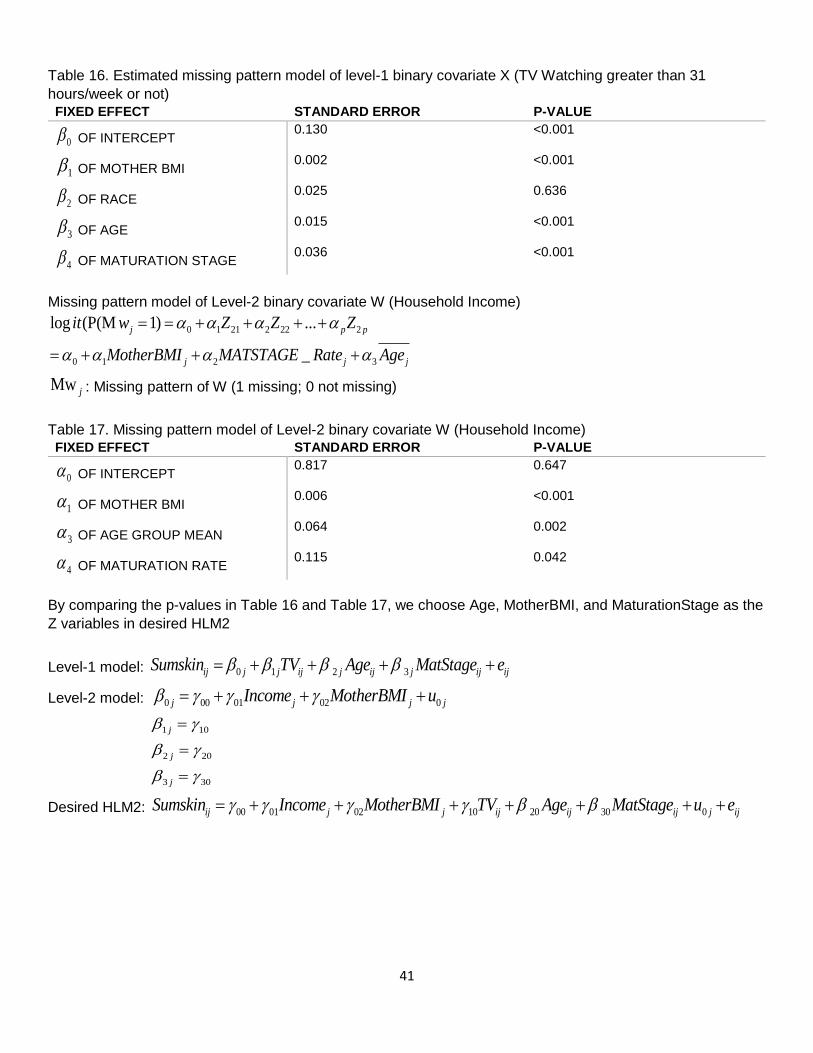
Table 16. Estimated missing pattern model of level-1 binary covariate X (TV Watching greater than 31
hours/week or not) FIXED EFFECT STANDARD ERROR P-VALUE
0 OF INTERCEPT 0.130 <0.001
1 OF MOTHER BMI 0.002 <0.001
2 OF RACE 0.025 0.636
3 OF AGE 0.015 <0.001
4 OF MATURATION STAGE 0.036 <0.001
Missing pattern model of Level-2 binary covariate W (Household Income)
0 1 21 2 22 2
0 1 2 3
log (P(M 1) ...
_
j p p
j j j
it w Z Z Z
MotherBMI MATSTAGE Rate Age
Mw j : Missing pattern of W (1 missing; 0 not missing)
Table 17. Missing pattern model of Level-2 binary covariate W (Household Income)
FIXED EFFECT STANDARD ERROR P-VALUE
0 OF INTERCEPT 0.817 0.647
1 OF MOTHER BMI 0.006 <0.001
3 OF AGE GROUP MEAN 0.064 0.002
4 OF MATURATION RATE 0.115 0.042
By comparing the p-values in Table 16 and Table 17, we choose Age, MotherBMI, and MaturationStage as the
Z variables in desired HLM2
Level-1 model: 0 1 2 3ij j j ij j ij j ij ijSumskin TV Age MatStage e
Level-2 model: 0 00 01 02 0j j j jIncome MotherBMI u
1 10
2 20
3 30
j
j
j
Desired HLM2: 00 01 02 10 20 30 0ij j j ij ij ij j ijSumskin Income MotherBMI TV Age MatStage u e
42
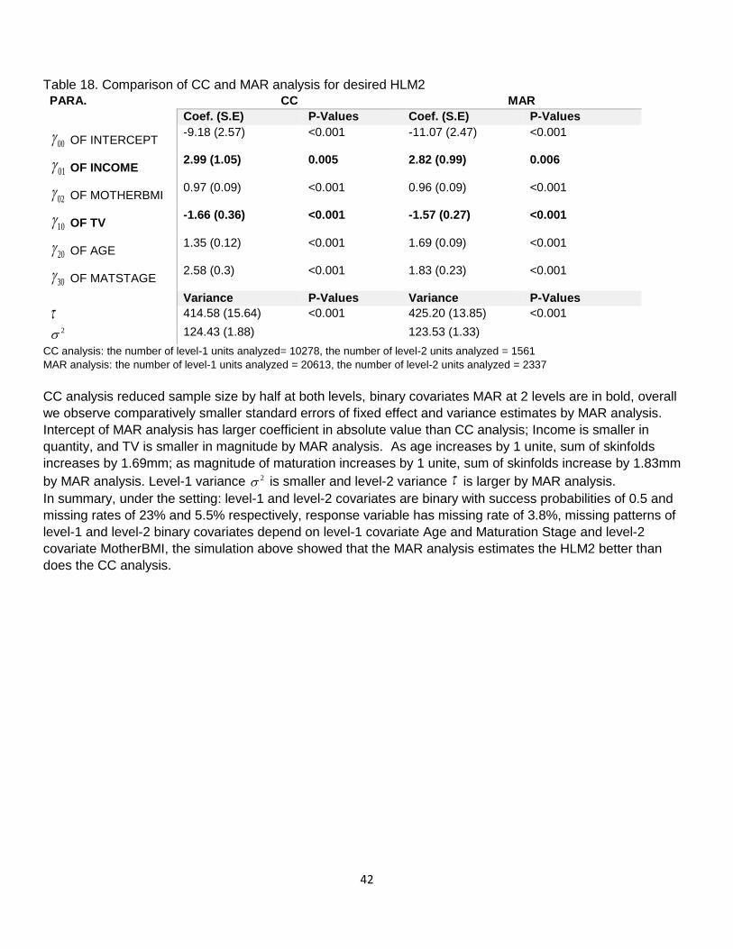
Table 18. Comparison of CC and MAR analysis for desired HLM2
PARA. CC MAR
Coef. (S.E) P-Values Coef. (S.E) P-Values
00 OF INTERCEPT -9.18 (2.57) <0.001 -11.07 (2.47) <0.001
01 OF INCOME 2.99 (1.05) 0.005 2.82 (0.99) 0.006
02 OF MOTHERBMI 0.97 (0.09) <0.001 0.96 (0.09) <0.001
10 OF TV -1.66 (0.36) <0.001 -1.57 (0.27) <0.001
20 OF AGE 1.35 (0.12) <0.001 1.69 (0.09) <0.001
30 OF MATSTAGE 2.58 (0.3) <0.001 1.83 (0.23) <0.001
Variance P-Values Variance P-Values
414.58 (15.64) <0.001 425.20 (13.85) <0.001
2 124.43 (1.88) 123.53 (1.33)
CC analysis: the number of level-1 units analyzed= 10278, the number of level-2 units analyzed = 1561
MAR analysis: the number of level-1 units analyzed = 20613, the number of level-2 units analyzed = 2337
CC analysis reduced sample size by half at both levels, binary covariates MAR at 2 levels are in bold, overall
we observe comparatively smaller standard errors of fixed effect and variance estimates by MAR analysis.
Intercept of MAR analysis has larger coefficient in absolute value than CC analysis; Income is smaller in
quantity, and TV is smaller in magnitude by MAR analysis. As age increases by 1 unite, sum of skinfolds
increases by 1.69mm; as magnitude of maturation increases by 1 unite, sum of skinfolds increase by 1.83mm
by MAR analysis. Level-1 variance 2 is smaller and level-2 variance is larger by MAR analysis.
In summary, under the setting: level-1 and level-2 covariates are binary with success probabilities of 0.5 and
missing rates of 23% and 5.5% respectively, response variable has missing rate of 3.8%, missing patterns of
level-1 and level-2 binary covariates depend on level-1 covariate Age and Maturation Stage and level-2
covariate MotherBMI, the simulation above showed that the MAR analysis estimates the HLM2 better than
does the CC analysis.

43
List of Tables Table 1 Comparison of 100
Bias
of fixed and random estimators among complete-data (CD), the MAR (MAR), and complete-case (CC) analysis
00 01 10
2
MW MX PW PX CD MAR CC CD MAR CC CD MAR CC CD MAR CC CD MAR CC
0.1 0.1 0.1 0.1 -.02 0.5 15.3 0 -4.8 -6.3 -.35 -0.6 -6.8 -.06 3.8 -12.2 .01 -0.1 -6.5
0.3 -.03 0.2 15.0 0 -4.3 -6.7 -.01 -0.5 -6.7 -.03 6.6 -6.0 0 0.1 -6.1
0.5 -.04 0.1 15.7 0 -5.2 -4.7 .11 -0.1 -8.1 -.03 5.8 -8.0 0 1.2 -6.1
0.3 0.1 -.03 0.2 15.7 0 -3.5 -8.1 -.03 -0.2 -6.7 -.03 9.3 -7.0 .01 -0.1 -5.6
0.3 -.03 0.9 15.2 -.04 -5.5 -7.5 .03 -0.6 -5.6 -.03 11.7 -7.0 0 0.2 -5.5
0.5 -.01 0.4 14.5 -.02 -3.7 -6.6 -.05 0.8 -5.2 -.03 12.9 -7.0 0 3.2 -5.3
0.5 0.1 -.04 0.4 14.4 .11 -3.1 -5.6 0 -0.2 -5.8 -.03 11.3 -7.0 0 -0.1 -5.0
0.3 -.01 -0.5 14.2 .12 -2.5 -6.2 .07 0.5 -5.2 -.03 14.4 -5.0 .01 0.1 -4.9
0.5 -.09 0.5 14.9 .17 -3.0 -7.0 -.04 -0.3 -5.5 -.03 11.1 -7.0 0 -0.1 -4.7
0.3 0.1 0.1 0.1 -.02 0.3 17.1 0 -14.4 -7.1 -.35 0.4 -6.7 -.06 15.0 -13.3 .01 0.0 -6.3
0.3 -.03 0.8 17.6 0 -16.2 -6.2 -.01 0.1 -6.7 -.03 14.7 -11.0 0 0.0 -6.3
0.5 -.04 0.3 17.6 0 -13.6 -8.4 .11 0.0 -7.2 -.03 14.3 -9.0 0 4.7 -5.6
0.3 0.1 -.03 0.7 17.0 0 -11.5 -7.0 -.03 0.2 -6.4 -.03 26.0 -8.0 .01 0.0 -5.7
0.3 -.03 1.3 17.4 -.04 -11.3 -7.5 .03 -0.5 -6.1 -.03 26.4 -8.0 0 0.1 -5.7
0.5 -.01 1.1 16.5 -.02 -8.6 -6.4 -.05 -0.3 -5.5 -.03 30.4 -8.0 0 8.3 -5.5
0.5 0.1 -.04 1.6 16.7 .11 -8.6 -7.1 0 -0.2 -5.6 -.03 28.5 -7.0 0 -0.1 -5.0
0.3 -.01 2.3 16.9 .12 -10.5 -8.3 .07 -0.2 -5.1 -.03 32.4 -8.0 .01 0.2 -5.0
0.5 -.09 1.5 16.6 .17 -8.4 -6.9 -.04 -0.2 -5.4 -.03 28.3 -6.0 0 -0.1 -4.5
0.5 0.1 0.1 0.1 -.02 2.0 19.1 0 -28.1 -7.5 -.35 -0.2 -6.7 -.06 21.2 -14.0 .01 0.1 -6.3
0.3 -.03 2.1 18.3 0 -27.4 -4.9 -.01 -0.4 -5.8 -.03 22.1 -9.0 0 0.1 -6.3
0.5 -.04 1.8 19.1 0 -26.4 -6.1 .11 -0.6 -6.7 -.03 21.1 -14.0 0 6.7 -5.6
0.3 0.1 -.03 2.5 19.2 0 -17.7 -8.2 -.03 -0.3 -5.5 -.03 37.1 -10.0 .01 -0.1 -5.6
0.3 -.03 1.9 19.0 -.04 -17.2 -8.4 .03 0.4 -5.9 -.03 40.0 -11.0 0 0.1 -5.2
0.5 -.01 4.6 19.0 -.02 -15.8 -7.2 -.05 0.0 -5.6 -.03 45.5 -7.0 0 11.8 -5.1
0.5 0.1 -.04 4.0 18.7 .11 -15.0 -8.5 0 -0.5 -5.8 -.03 43.8 -10.0 0 0.0 -4.4
0.3 -.01 5.3 19.2 .12 -17.7 -9.2 .07 -0.3 -5.3 -.03 47.3 -9.0 .01 0.1 -5.1
0.5 -.09 3.7 18.8 .17 -14.8 -8.4 -.04 -0.2 -5.2 -.03 43.7 -9.0 0 0.0 -4.6

44
00 01 10 2
MW MX PW PX CD MAR CC CD MAR CC CD MAR CC CD MAR CC CD MAR CC
0.1 0.3 0.1 0.1 -.02 0.5 30.9 0 -5.6 -11.0 -.35 -0.6 -11.7 -.06 4.6 -16.8 .01 -0.1 -11.3
0.3 -.03 0.3 30.6 0 -6.2 -8.5 -.01 -0.5 -11.6 -.03 7.3 -13.0 0 0.1 -10.9
0.5 -.04 -0.2 30.7 0 -4.9 -11.0 .11 -0.2 -11.2 -.03 6.4 -11.0 0 1.5 -11.1
0.3 0.1 -.03 0.4 31.1 0 -4.2 -12.3 -.03 -0.4 -12.0 -.03 11.0 -12.0 .01 0.1 -10.2
0.3 -.03 0.0 31.2 -.04 -2.9 -12.8 .03 -0.8 -11.0 -.03 11.4 -13.0 0 0.2 -10.2
0.5 -.01 0.4 30.2 -.02 -3.5 -11.2 -.05 0.2 -10.6 -.03 13.2 -13.0 0 3.5 -10.3
0.5 0.1 -.04 -0.1 29.8 .11 -2.3 -11.1 0 -0.3 -9.4 -.03 13.7 -10.0 0 0.1 -9.5
0.3 -.01 1.7 30.1 .12 -4.9 -11.6 .07 -1.1 -9.7 -.03 12.7 -11.0 .01 0.1 -9.4
0.5 -.09 0.5 29.6 .17 -2.9 -10.4 -.04 -0.5 -9.8 -.03 11.3 -13.0 0 0.1 -9.1
0.3 0.3 0.1 0.1 -.02 1.1 32.6 0 -16.0 -11.8 -.35 -0.6 -11.7 -.06 12.3 -17.9 .01 -0.1 -11.1
0.3 -.03 1.2 33.0 0 -16.9 -12.7 -.01 -1.3 -11.8 -.03 16.0 -14.0 0 0.1 -10.5
0.5 -.04 0.8 33.2 0 -17.3 -12.3 .11 -0.4 -11.5 -.03 14.8 -14.0 0 3.9 -11.1
0.3 0.1 -.03 1.1 32.4 0 -9.6 -13.0 -.03 -1.4 -10.2 -.03 25.6 -13.0 .01 0.2 -10.1
0.3 -.03 0.8 32.7 -.04 -11.0 -12.6 .03 0.5 -11.6 -.03 27.5 -11.0 0 0.0 -9.9
0.5 -.01 1.8 32.5 -.02 -8.5 -11.9 -.05 -0.7 -10.9 -.03 31.4 -13.0 0 8.1 -10.0
0.5 0.1 -.04 1.7 33.1 .11 -9.3 -13.3 0 0.3 -10.5 -.03 30.4 -13.0 0 0.1 -9.7
0.3 -.01 1.9 31.4 .12 -8.8 -11.3 .07 -1.0 -9.1 -.03 31.1 -14.0 .01 0.1 -9.5
0.5 -.09 1.6 32.4 .17 -8.6 -12.9 -.04 -0.4 -9.5 -.03 28.7 -13.0 0 0.1 -9.2
0.5 0.3 0.1 0.1 -.02 2.0 34.4 0 -27.1 -12.1 -.35 -0.6 -11.7 -.06 19.3 -18.4 .01 -0.1 -11.0
0.3 -.03 1.5 35.0 0 -26.2 -13.1 -.01 0.0 -11.4 -.03 20.4 -13.0 0 0.2 -10.8
0.5 -.04 2.1 33.9 0 -28.1 -8.7 .11 -0.7 -11.8 -.03 21.2 -17.0 0 6.1 -11.0
0.3 0.1 -.03 3.3 34.8 0 -18.3 -11.1 -.03 -1.3 -11.4 -.03 38.5 -12.0 .01 0.2 -10.4
0.3 -.03 3.9 32.4 -.04 -19.6 -9.9 .03 -1.1 -10.0 -.03 39.0 -14.0 0 0.1 -9.8
0.5 -.01 4.0 33.9 -.02 -15.8 -11.8 -.05 0.0 -11.5 -.03 46.8 -15.0 0 12.3 -9.6
0.5 0.1 -.04 4.4 34.4 .11 -16.6 -14.3 0 1.2 -8.7 -.03 44.5 -13.0 0 0.0 -9.3
0.3 -.01 4.4 33.3 .12 -15.8 -11.8 .07 -0.9 -9.3 -.03 46.6 -11.0 .01 0.2 -9.1
0.5 -.09 3.8 33.5 .17 -14.9 -12.6 -.04 -0.4 -9.1 -.03 44.0 -15.0 0 0.0 -9.1

45
00 01 10 2
MW MX PW PX CD MAR CC CD MAR CC CD MAR CC CD MAR CC CD MAR CC
0.1 0.5 0.1 0.1 -.02 0.4 43.9 0 -5.6 -13.8 -.35 -0.3 -14.6 -.06 4.5 -18.1 .01 -0.1 -14.0
0.3 -.03 0.5 44.4 0 -6.3 -14.9 -.01 -0.7 -15.1 -.03 6.0 -15.0 0 0.1 -14.2
0.5 -.04 0.4 43.1 0 -5.5 -13.0 .11 -0.7 -13.7 -.03 7.8 -13.0 0 1.4 -13.5
0.3 0.1 -.03 0.8 43.9 0 -4.5 -14.0 -.03 -1.0 -13.9 -.03 11.6 -15.0 .01 0.3 -13.2
0.3 -.03 -0.6 43.3 -.04 -2.3 -13.5 .03 0.2 -13.9 -.03 11.2 -15.0 0 0.0 -13.1
0.5 -.01 0.8 44.1 -.02 -3.7 -14.5 -.05 -1.0 -14.1 -.03 12.9 -17.0 0 3.8 -12.9
0.5 0.1 -.04 0.5 43.6 .11 -2.9 -15.0 0 -0.5 -12.9 -.03 11.2 -14.0 0 0.0 -12.4
0.3 -.01 0.3 43.1 .12 -2.5 -14.1 .07 -0.9 -12.6 -.03 13.0 -13.0 .01 0.2 -12.8
0.5 -.09 0.5 43.4 .17 -2.9 -14.0 -.04 -0.6 -13.9 -.03 11.1 -13.0 0 0.0 -12.1
0.3 0.5 0.1 0.1 -.02 1.0 46.3 0 -16.1 -14.5 -.35 -0.6 -14.8 -.06 12.3 -19.0 .01 0.0 -13.1
0.3 -.03 0.6 45.8 0 -14.0 -16.8 -.01 -0.9 -14.0 -.03 15.0 -18.0 0 0.2 -13.6
0.5 -.04 0.5 45.2 0 -14.7 -16.2 .11 0.0 -13.7 -.03 13.5 -17.0 0 3.9 -13.4
0.3 0.1 -.03 1.9 44.8 0 -11.5 -13.8 -.03 -1.2 -13.5 -.03 25.7 -17.0 .01 0.1 -12.7
0.3 -.03 0.6 46.1 -.04 -9.9 -14.3 .03 -0.3 -14.5 -.03 27.9 -18.0 0 0.0 -13.0
0.5 -.01 1.3 46.7 -.02 -8.3 -16.4 -.05 -0.6 -14.6 -.03 32.3 -16.0 0 8.2 -12.9
0.5 0.1 -.04 1.6 45.2 .11 -8.3 -14.1 0 -0.7 -13.7 -.03 28.6 -16.0 0 0.0 -12.4
0.3 -.01 2.5 45.7 .12 -9.6 -16.1 .07 -1.3 -12.6 -.03 30.9 -12.0 .01 0.2 -12.3
0.5 -.09 1.8 45.1 .17 -8.6 -14.3 -.04 -0.6 -13.8 -.03 28.7 -16.0 0 0.0 -12.1
0.5 0.5 0.1 0.1 -.02 2.0 47.4 0 -27.1 -16.1 -.35 -0.6 -14.2 -.06 19.6 -20.0 .01 0.0 -13.4
0.3 -.03 1.1 47.9 0 -27.1 -14.9 -.01 0.3 -14.9 -.03 21.1 -21.0 0 0.0 -13.5
0.5 -.04 0.8 48.0 0 -8.3 -16.2 .11 -1.3 -14.6 -.03 6.7 -19.0 0 6.2 -13.1
0.3 0.1 -.03 3.1 46.4 0 -19.1 -14.4 -.03 0.9 -13.7 -.03 39.0 -13.0 .01 0.0 -12.6
0.3 -.03 3.6 45.9 -.04 -19.9 -15.4 .03 -0.4 -12.1 -.03 40.0 -16.0 0 0.1 -12.8
0.5 -.01 3.9 45.7 -.02 -15.1 -14.3 -.05 -0.5 -12.6 -.03 43.9 -12.0 0 12.4 -12.8
0.5 0.1 -.04 4.0 47.4 .11 -15.0 -17.2 0 -0.7 -12.9 -.03 43.7 -15.0 0 0.0 -11.9
0.3 -.01 4.3 46.1 .12 -16.6 -14.0 .07 0.0 -13.6 -.03 45.7 -19.0 .01 0.0 -12.1
0.5 -.09 4.0 46.3 .17 -15.0 -15.0 -.04 -0.5 -12.5 -.03 43.9 -15.0 0 0.0 -12.2
MX: Missing rate of X
MW: Missing rate of W
PX: Success probability of X
Pw: Success probability of W
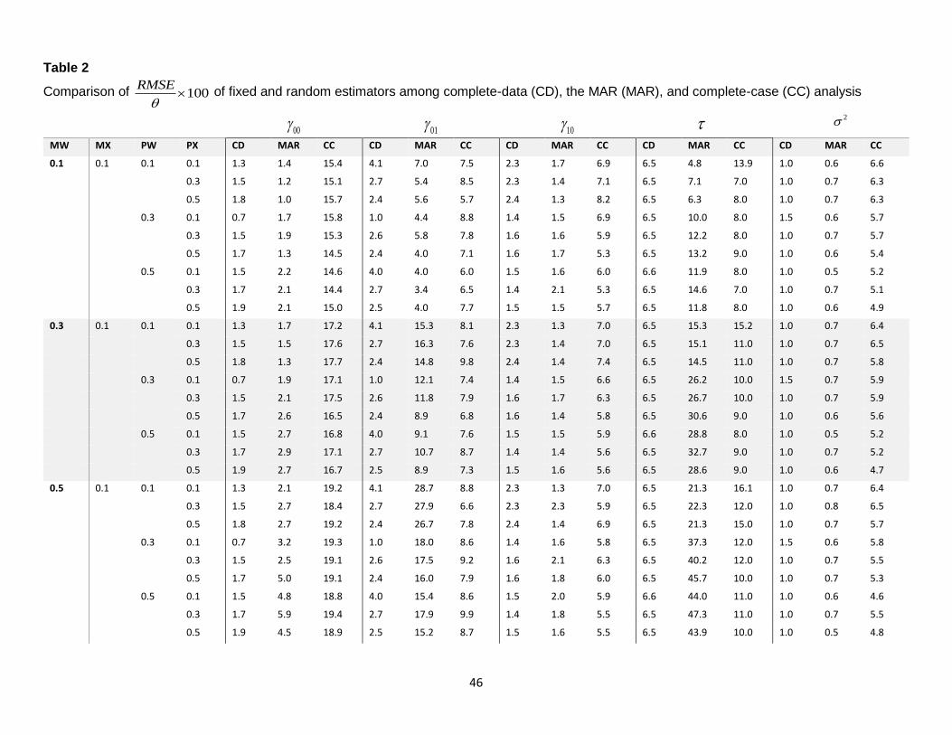
46
Table 2
Comparison of 100RMSE
of fixed and random estimators among complete-data (CD), the MAR (MAR), and complete-case (CC) analysis
00 01 10
2
MW MX PW PX CD MAR CC CD MAR CC CD MAR CC CD MAR CC CD MAR CC
0.1 0.1 0.1 0.1 1.3 1.4 15.4 4.1 7.0 7.5 2.3 1.7 6.9 6.5 4.8 13.9 1.0 0.6 6.6
0.3 1.5 1.2 15.1 2.7 5.4 8.5 2.3 1.4 7.1 6.5 7.1 7.0 1.0 0.7 6.3
0.5 1.8 1.0 15.7 2.4 5.6 5.7 2.4 1.3 8.2 6.5 6.3 8.0 1.0 0.7 6.3
0.3 0.1 0.7 1.7 15.8 1.0 4.4 8.8 1.4 1.5 6.9 6.5 10.0 8.0 1.5 0.6 5.7
0.3 1.5 1.9 15.3 2.6 5.8 7.8 1.6 1.6 5.9 6.5 12.2 8.0 1.0 0.7 5.7
0.5 1.7 1.3 14.5 2.4 4.0 7.1 1.6 1.7 5.3 6.5 13.2 9.0 1.0 0.6 5.4
0.5 0.1 1.5 2.2 14.6 4.0 4.0 6.0 1.5 1.6 6.0 6.6 11.9 8.0 1.0 0.5 5.2
0.3 1.7 2.1 14.4 2.7 3.4 6.5 1.4 2.1 5.3 6.5 14.6 7.0 1.0 0.7 5.1
0.5 1.9 2.1 15.0 2.5 4.0 7.7 1.5 1.5 5.7 6.5 11.8 8.0 1.0 0.6 4.9
0.3 0.1 0.1 0.1 1.3 1.7 17.2 4.1 15.3 8.1 2.3 1.3 7.0 6.5 15.3 15.2 1.0 0.7 6.4
0.3 1.5 1.5 17.6 2.7 16.3 7.6 2.3 1.4 7.0 6.5 15.1 11.0 1.0 0.7 6.5
0.5 1.8 1.3 17.7 2.4 14.8 9.8 2.4 1.4 7.4 6.5 14.5 11.0 1.0 0.7 5.8
0.3 0.1 0.7 1.9 17.1 1.0 12.1 7.4 1.4 1.5 6.6 6.5 26.2 10.0 1.5 0.7 5.9
0.3 1.5 2.1 17.5 2.6 11.8 7.9 1.6 1.7 6.3 6.5 26.7 10.0 1.0 0.7 5.9
0.5 1.7 2.6 16.5 2.4 8.9 6.8 1.6 1.4 5.8 6.5 30.6 9.0 1.0 0.6 5.6
0.5 0.1 1.5 2.7 16.8 4.0 9.1 7.6 1.5 1.5 5.9 6.6 28.8 8.0 1.0 0.5 5.2
0.3 1.7 2.9 17.1 2.7 10.7 8.7 1.4 1.4 5.6 6.5 32.7 9.0 1.0 0.7 5.2
0.5 1.9 2.7 16.7 2.5 8.9 7.3 1.5 1.6 5.6 6.5 28.6 9.0 1.0 0.6 4.7
0.5 0.1 0.1 0.1 1.3 2.1 19.2 4.1 28.7 8.8 2.3 1.3 7.0 6.5 21.3 16.1 1.0 0.7 6.4
0.3 1.5 2.7 18.4 2.7 27.9 6.6 2.3 2.3 5.9 6.5 22.3 12.0 1.0 0.8 6.5
0.5 1.8 2.7 19.2 2.4 26.7 7.8 2.4 1.4 6.9 6.5 21.3 15.0 1.0 0.7 5.7
0.3 0.1 0.7 3.2 19.3 1.0 18.0 8.6 1.4 1.6 5.8 6.5 37.3 12.0 1.5 0.6 5.8
0.3 1.5 2.5 19.1 2.6 17.5 9.2 1.6 2.1 6.3 6.5 40.2 12.0 1.0 0.7 5.5
0.5 1.7 5.0 19.1 2.4 16.0 7.9 1.6 1.8 6.0 6.5 45.7 10.0 1.0 0.7 5.3
0.5 0.1 1.5 4.8 18.8 4.0 15.4 8.6 1.5 2.0 5.9 6.6 44.0 11.0 1.0 0.6 4.6
0.3 1.7 5.9 19.4 2.7 17.9 9.9 1.4 1.8 5.5 6.5 47.3 11.0 1.0 0.7 5.5
0.5 1.9 4.5 18.9 2.5 15.2 8.7 1.5 1.6 5.5 6.5 43.9 10.0 1.0 0.5 4.8

47
00 01 10
2
MW MX PW PX CD MAR CC CD MAR CC CD MAR CC CD MAR CC CD MAR CC
0.1 0.3 0.1 0.1 1.3 1.7 30.9 4.1 7.0 11.7 2.3 1.9 11.9 6.5 5.9 18.2 1.0 0.6 11.3
0.3 1.5 1.8 30.6 2.7 7.4 9.1 2.3 2.0 11.7 6.5 7.8 13.0 1.0 0.9 11.0
0.5 1.8 1.4 30.8 2.4 7.1 11.5 2.4 1.5 11.3 6.5 6.6 12.0 1.0 0.8 11.2
0.3 0.1 0.7 1.6 31.2 1.0 5.1 12.8 1.4 2.4 12.4 6.5 11.2 14.0 1.5 0.8 10.3
0.3 1.5 1.6 31.3 2.6 3.4 13.2 1.6 1.7 11.2 6.5 11.7 13.0 1.0 1.0 10.3
0.5 1.7 1.9 30.2 2.4 4.1 11.4 1.6 1.7 10.7 6.5 13.4 15.0 1.0 0.8 10.4
0.5 0.1 1.5 2.2 29.8 4.0 3.3 11.3 1.5 1.2 9.7 6.6 14.0 10.0 1.0 0.6 9.6
0.3 1.7 3.1 30.1 2.7 5.7 11.8 1.4 2.0 9.7 6.5 13.0 12.0 1.0 0.7 9.5
0.5 1.9 2.2 29.7 2.5 3.9 10.7 1.5 1.8 10.0 6.5 12.0 14.0 1.0 0.6 9.2
0.3 0.3 0.1 0.1 1.3 1.9 32.7 4.1 16.6 12.5 2.3 1.9 11.9 6.5 12.8 19.3 1.0 0.6 11.2
0.3 1.5 1.9 33.0 2.7 17.2 13.3 2.3 1.8 12.0 6.5 16.2 15.0 1.0 0.6 10.6
0.5 1.8 1.5 33.2 2.4 17.8 12.6 2.4 2.6 11.6 6.5 14.8 15.0 1.0 0.7 11.2
0.3 0.1 0.7 1.6 32.5 1.0 10.0 13.5 1.4 1.8 10.4 6.5 25.8 14.0 1.5 0.8 10.3
0.3 1.5 1.7 32.8 2.6 11.2 12.7 1.6 1.6 11.7 6.5 27.8 12.0 1.0 0.8 10.0
0.5 1.7 2.5 32.5 2.4 8.9 12.0 1.6 2.6 11.0 6.5 31.6 14.0 1.0 0.8 10.2
0.5 0.1 1.5 2.6 33.2 4.0 9.6 13.7 1.5 1.8 10.6 6.6 30.6 15.0 1.0 0.8 9.8
0.3 1.7 3.5 31.4 2.7 9.5 11.5 1.4 2.2 9.2 6.5 31.2 14.0 1.0 0.8 9.7
0.5 1.9 2.8 32.5 2.5 9.1 13.4 1.5 1.8 9.7 6.5 29.0 14.0 1.0 0.6 9.3
0.5 0.3 0.1 0.1 1.3 2.6 34.5 4.1 27.6 13.0 2.3 1.9 11.9 6.5 19.7 20.2 1.0 0.6 11.1
0.3 1.5 2.1 35.0 2.7 26.3 14.2 2.3 1.2 11.5 6.5 20.7 15.0 1.0 1.0 10.9
0.5 1.8 2.4 34.0 2.4 28.8 9.7 2.4 2.5 12.0 6.5 21.4 17.0 1.0 0.7 11.1
0.3 0.1 0.7 3.6 34.9 1.0 18.7 11.4 1.4 2.2 11.5 6.5 38.8 13.0 1.5 0.8 10.5
0.3 1.5 4.6 32.5 2.6 20.0 10.2 1.6 2.1 10.2 6.5 39.2 16.0 1.0 0.9 9.9
0.5 1.7 4.5 33.9 2.4 16.0 12.3 1.6 1.0 11.6 6.5 47.1 16.0 1.0 0.8 9.7
0.5 0.1 1.5 5.0 34.5 4.0 16.9 14.6 1.5 2.3 9.0 6.6 44.5 14.0 1.0 0.8 9.4
0.3 1.7 4.6 33.3 2.7 15.9 12.1 1.4 1.9 9.4 6.5 46.7 14.0 1.0 0.9 9.2
0.5 1.9 4.6 33.6 2.5 15.3 12.8 1.5 1.8 9.3 6.5 44.2 16.0 1.0 0.6 9.3
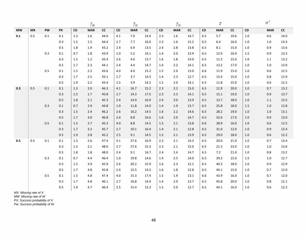
48
00 01 10
2
MW MX PW PX CD MAR CC CD MAR CC CD MAR CC CD MAR CC CD MAR CC
0.1 0.5 0.1 0.1 1.3 1.6 44.0 4.1 7.0 14.4 2.3 1.6 14.7 6.5 5.7 19.6 1.0 0.6 14.0
0.3 1.5 1.5 44.4 2.7 7.7 16.0 2.3 1.6 15.2 6.5 6.4 16.0 1.0 1.0 14.3
0.5 1.8 1.9 43.2 2.4 6.9 13.5 2.4 2.8 13.8 6.5 8.1 15.0 1.0 0.9 13.6
0.3 0.1 0.7 1.8 43.9 1.0 5.2 14.1 1.4 2.0 13.9 6.5 12.0 16.0 1.5 0.9 13.3
0.3 1.5 1.2 43.4 2.6 4.0 13.7 1.6 1.8 14.0 6.5 11.5 15.0 1.0 1.1 13.2
0.5 1.7 2.3 44.1 2.4 4.4 14.7 1.6 2.2 14.1 6.5 13.2 17.0 1.0 1.0 13.0
0.5 0.1 1.5 2.2 43.6 4.0 4.0 15.2 1.5 2.0 13.0 6.6 11.9 15.0 1.0 0.6 12.5
0.3 1.7 2.5 43.1 2.7 3.7 14.3 1.4 2.3 12.7 6.5 13.4 15.0 1.0 0.8 12.9
0.5 1.9 2.2 43.4 2.5 3.9 14.2 1.5 2.0 14.1 6.5 11.8 15.0 1.0 0.6 12.2
0.3 0.5 0.1 0.1 1.3 2.0 46.3 4.1 16.7 15.2 2.3 2.2 15.0 6.5 12.9 20.0 1.0 0.7 13.2
0.3 1.5 1.7 45.8 2.7 14.3 17.5 2.3 2.3 14.1 6.5 15.1 19.0 1.0 0.9 13.7
0.5 1.8 2.1 45.3 2.4 14.9 16.9 2.4 3.0 13.9 6.5 13.7 18.0 1.0 1.1 13.5
0.3 0.1 0.7 2.9 44.8 1.0 11.8 14.0 1.4 1.9 13.7 6.5 25.8 18.0 1.5 1.0 12.8
0.3 1.5 2.4 46.2 2.6 10.2 14.5 1.6 2.2 14.6 6.5 28.2 19.0 1.0 1.0 13.1
0.5 1.7 3.0 46.8 2.4 8.8 16.6 1.6 2.0 14.7 6.5 32.6 17.0 1.0 0.9 13.0
0.5 0.1 1.5 2.7 45.3 4.0 8.8 14.5 1.5 2.1 13.8 6.6 28.9 16.0 1.0 0.6 12.5
0.3 1.7 3.2 45.7 2.7 10.1 16.4 1.4 2.1 12.8 6.5 31.0 12.0 1.0 0.9 12.4
0.5 1.9 2.8 45.2 2.5 9.1 14.5 1.5 2.1 13.9 6.5 29.0 18.0 1.0 0.6 12.2
0.5 0.5 0.1 0.1 1.3 2.6 47.4 4.1 27.6 16.9 2.3 2.1 14.3 6.5 20.0 21.0 1.0 0.7 13.4
0.3 1.5 2.1 48.0 2.7 27.6 15.3 2.3 2.1 15.0 6.5 21.3 23.0 1.0 1.0 13.6
0.5 1.8 1.8 48.0 2.4 9.1 16.7 2.4 2.4 14.7 6.5 7.2 21.0 1.0 0.8 13.2
0.3 0.1 0.7 4.4 46.4 1.0 19.8 14.6 1.4 2.5 14.0 6.5 39.2 15.0 1.5 1.0 12.7
0.3 1.5 3.9 45.9 2.6 20.2 15.9 1.6 2.3 12.1 6.5 40.2 18.0 1.0 0.9 12.9
0.5 1.7 4.8 45.8 2.4 15.5 14.5 1.6 1.8 12.8 6.5 44.1 15.0 1.0 0.7 12.9
0.5 0.1 1.5 4.8 47.4 4.0 15.3 17.4 1.5 1.9 13.1 6.6 43.9 16.0 1.0 0.7 12.0
0.3 1.7 4.8 46.1 2.7 16.8 14.4 1.4 2.0 13.7 6.5 45.8 20.0 1.0 0.8 12.1
0.5 1.9 4.7 46.4 2.5 15.4 15.3 1.5 2.0 12.7 6.5 44.1 16.0 1.0 0.6 12.2
MX: Missing rate of X
MW: Missing rate of W
PX: Success probability of X
Pw: Success probability of W
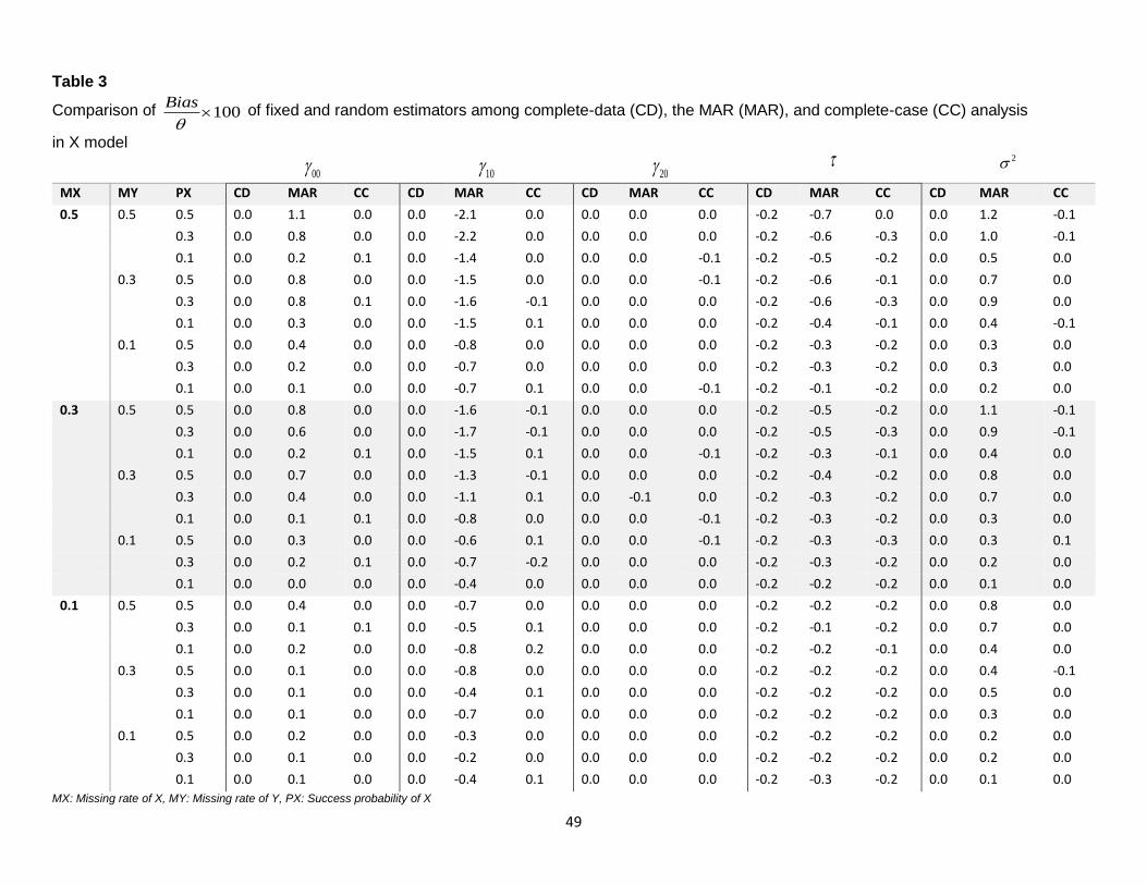
49
Table 3
Comparison of 100Bias
of fixed and random estimators among complete-data (CD), the MAR (MAR), and complete-case (CC) analysis
in X model
00 10 20 2
MX MY PX CD MAR CC CD MAR CC CD MAR CC CD MAR CC CD MAR CC
0.5 0.5 0.5 0.0 1.1 0.0 0.0 -2.1 0.0 0.0 0.0 0.0 -0.2 -0.7 0.0 0.0 1.2 -0.1
0.3 0.0 0.8 0.0 0.0 -2.2 0.0 0.0 0.0 0.0 -0.2 -0.6 -0.3 0.0 1.0 -0.1
0.1 0.0 0.2 0.1 0.0 -1.4 0.0 0.0 0.0 -0.1 -0.2 -0.5 -0.2 0.0 0.5 0.0
0.3 0.5 0.0 0.8 0.0 0.0 -1.5 0.0 0.0 0.0 -0.1 -0.2 -0.6 -0.1 0.0 0.7 0.0
0.3 0.0 0.8 0.1 0.0 -1.6 -0.1 0.0 0.0 0.0 -0.2 -0.6 -0.3 0.0 0.9 0.0
0.1 0.0 0.3 0.0 0.0 -1.5 0.1 0.0 0.0 0.0 -0.2 -0.4 -0.1 0.0 0.4 -0.1
0.1 0.5 0.0 0.4 0.0 0.0 -0.8 0.0 0.0 0.0 0.0 -0.2 -0.3 -0.2 0.0 0.3 0.0
0.3 0.0 0.2 0.0 0.0 -0.7 0.0 0.0 0.0 0.0 -0.2 -0.3 -0.2 0.0 0.3 0.0
0.1 0.0 0.1 0.0 0.0 -0.7 0.1 0.0 0.0 -0.1 -0.2 -0.1 -0.2 0.0 0.2 0.0
0.3 0.5 0.5 0.0 0.8 0.0 0.0 -1.6 -0.1 0.0 0.0 0.0 -0.2 -0.5 -0.2 0.0 1.1 -0.1
0.3 0.0 0.6 0.0 0.0 -1.7 -0.1 0.0 0.0 0.0 -0.2 -0.5 -0.3 0.0 0.9 -0.1
0.1 0.0 0.2 0.1 0.0 -1.5 0.1 0.0 0.0 -0.1 -0.2 -0.3 -0.1 0.0 0.4 0.0
0.3 0.5 0.0 0.7 0.0 0.0 -1.3 -0.1 0.0 0.0 0.0 -0.2 -0.4 -0.2 0.0 0.8 0.0
0.3 0.0 0.4 0.0 0.0 -1.1 0.1 0.0 -0.1 0.0 -0.2 -0.3 -0.2 0.0 0.7 0.0
0.1 0.0 0.1 0.1 0.0 -0.8 0.0 0.0 0.0 -0.1 -0.2 -0.3 -0.2 0.0 0.3 0.0
0.1 0.5 0.0 0.3 0.0 0.0 -0.6 0.1 0.0 0.0 -0.1 -0.2 -0.3 -0.3 0.0 0.3 0.1
0.3 0.0 0.2 0.1 0.0 -0.7 -0.2 0.0 0.0 0.0 -0.2 -0.3 -0.2 0.0 0.2 0.0
0.1 0.0 0.0 0.0 0.0 -0.4 0.0 0.0 0.0 0.0 -0.2 -0.2 -0.2 0.0 0.1 0.0
0.1 0.5 0.5 0.0 0.4 0.0 0.0 -0.7 0.0 0.0 0.0 0.0 -0.2 -0.2 -0.2 0.0 0.8 0.0
0.3 0.0 0.1 0.1 0.0 -0.5 0.1 0.0 0.0 0.0 -0.2 -0.1 -0.2 0.0 0.7 0.0
0.1 0.0 0.2 0.0 0.0 -0.8 0.2 0.0 0.0 0.0 -0.2 -0.2 -0.1 0.0 0.4 0.0
0.3 0.5 0.0 0.1 0.0 0.0 -0.8 0.0 0.0 0.0 0.0 -0.2 -0.2 -0.2 0.0 0.4 -0.1
0.3 0.0 0.1 0.0 0.0 -0.4 0.1 0.0 0.0 0.0 -0.2 -0.2 -0.2 0.0 0.5 0.0
0.1 0.0 0.1 0.0 0.0 -0.7 0.0 0.0 0.0 0.0 -0.2 -0.2 -0.2 0.0 0.3 0.0
0.1 0.5 0.0 0.2 0.0 0.0 -0.3 0.0 0.0 0.0 0.0 -0.2 -0.2 -0.2 0.0 0.2 0.0
0.3 0.0 0.1 0.0 0.0 -0.2 0.0 0.0 0.0 0.0 -0.2 -0.2 -0.2 0.0 0.2 0.0
0.1 0.0 0.1 0.0 0.0 -0.4 0.1 0.0 0.0 0.0 -0.2 -0.3 -0.2 0.0 0.1 0.0
MX: Missing rate of X, MY: Missing rate of Y, PX: Success probability of X

50
Table 4
Comparison of 100RMSE
of fixed and random estimators among complete-data (CD), the MAR (MAR), and complete-case (CC) analysis
in X model
00 10 20 2
MX MY PX CD MAR CC CD MAR CC CD MAR CC CD MAR CC CD MAR CC
0.5 0.5 0.5 3.3 4.2 4.1 1.7 4.6 3.6 0.8 1.3 1.8 4.7 5.3 5.9 1.0 2.4 2.2
0.3 3.4 3.9 4.0 1.7 4.9 3.6 0.8 1.3 1.8 4.7 5.3 5.9 1.0 2.5 2.2
0.1 3.3 3.5 3.9 2.1 6.2 4.5 0.8 1.2 1.7 4.8 5.4 5.8 1.0 2.2 2.2
0.3 0.5 3.3 3.9 3.9 1.7 3.6 3.1 0.8 1.1 1.6 4.7 5.2 5.4 1.0 1.9 1.8
0.3 3.4 3.9 3.7 1.7 3.6 3.0 0.8 1.1 1.5 4.7 5.2 5.4 1.0 2.1 1.8
0.1 3.3 3.4 3.7 2.1 5.1 3.9 0.8 1.1 1.6 4.8 5.0 5.5 1.0 1.7 1.9
0.1 0.5 3.3 3.5 3.7 1.7 2.8 2.6 0.8 0.9 1.3 4.7 4.8 5.1 1.0 1.4 1.6
0.3 3.4 3.5 3.6 1.7 3.0 2.7 0.8 0.9 1.3 4.7 4.9 5.1 1.0 1.5 1.6
0.1 3.3 3.4 3.6 2.1 4.1 3.3 0.8 0.8 1.3 4.8 4.7 5.2 1.0 1.3 1.6
0.3 0.5 0.5 3.3 4.2 4.0 1.7 4.0 3.2 0.8 1.2 1.5 4.7 5.4 5.7 1.0 2.4 1.9
0.3 3.4 3.6 3.8 1.7 4.3 3.2 0.8 1.2 1.5 4.7 5.4 5.6 1.0 2.2 1.9
0.1 3.3 3.6 3.7 2.1 5.4 4.1 0.8 1.2 1.5 4.8 5.3 5.6 1.0 2.1 1.8
0.3 0.5 3.3 3.7 3.7 1.7 3.1 2.6 0.8 1.0 1.3 4.7 5.1 5.2 1.0 1.8 1.6
0.3 3.4 3.6 3.6 1.7 3.2 2.7 0.8 1.1 1.3 4.7 5.0 5.3 1.0 1.8 1.6
0.1 3.3 3.4 3.6 2.1 4.3 3.4 0.8 1.1 1.3 4.8 5.0 5.3 1.0 1.6 1.6
0.1 0.5 3.3 3.4 3.5 1.7 2.3 2.2 0.8 0.9 1.1 4.7 4.8 5.1 1.0 1.3 1.4
0.3 3.4 3.4 3.5 1.7 2.5 2.3 0.8 0.9 1.1 4.7 4.8 5.0 1.0 1.3 1.4
0.1 3.3 3.3 3.4 2.1 3.4 3.0 0.8 0.8 1.1 4.8 4.8 5.0 1.0 1.2 1.4
0.1 0.5 0.5 3.3 3.8 3.6 1.7 3.2 2.7 0.8 1.2 1.2 4.7 5.2 5.3 1.0 2.1 1.5
0.3 3.4 3.6 3.7 1.7 3.2 2.5 0.8 1.2 1.2 4.7 5.3 5.4 1.0 2.1 1.5
0.1 3.3 3.6 3.6 2.1 4.6 3.4 0.8 1.2 1.2 4.8 5.2 5.3 1.0 1.9 1.5
0.3 0.5 3.3 3.6 3.5 1.7 4.6 2.2 0.8 1.2 1.0 4.7 5.1 5.0 1.0 1.9 1.3
0.3 3.4 3.4 3.5 1.7 2.5 2.3 0.8 1.0 1.1 4.7 5.0 5.0 1.0 1.6 1.4
0.1 3.3 3.4 3.4 2.1 3.7 3.0 0.8 1.0 1.1 4.8 4.9 5.1 1.0 1.5 1.3
0.1 0.5 3.3 3.4 3.4 1.7 1.9 1.9 0.8 0.8 0.9 4.7 4.8 4.9 1.0 1.2 1.2
0.3 3.4 3.4 3.4 1.7 2.0 2.0 0.8 0.8 0.9 4.7 4.8 4.9 1.0 1.2 1.2
0.1 3.3 3.1 3.3 2.1 2.6 2.5 0.8 0.8 0.9 4.8 4.7 4.9 1.0 1.1 1.1 MX: Missing rate of X, MY: Missing rate of Y, PX: Success probability of X

51
Table 5
Comparison of . 100S E of fixed and random estimators among complete-data (CD), the MAR (MAR), and complete-case (CC) analysis
in X model
00 10 20 2
MX MY PX CD MAR CC CD MAR CC CD MAR CC CD MAR CC CD MAR CC
0.5 0.5 0.5 3.3 3.8 4.2 1.7 3.0 3.5 0.8 1.3 1.8 4.7 5.2 5.9 1.0 1.8 2.2
0.3 3.3 3.6 4.0 1.7 3.1 3.6 0.8 1.2 1.8 4.7 5.1 5.9 1.0 1.7 2.2
0.1 3.3 3.5 3.9 2.2 4.2 4.5 0.8 1.2 1.7 4.7 5.1 5.9 1.0 1.6 2.2
0.3 0.5 3.3 3.6 3.9 1.7 2.6 3.0 0.8 1.1 1.5 4.7 4.9 5.5 1.0 1.5 1.9
0.3 3.3 3.6 3.8 1.7 2.6 3.1 0.8 1.1 1.5 4.7 4.9 5.5 1.0 1.5 1.9
0.1 3.3 3.4 3.7 2.2 3.8 3.9 0.8 1.0 1.5 4.7 4.9 5.5 1.0 1.4 1.9
0.1 0.5 3.3 3.5 3.7 1.7 2.3 2.6 0.8 0.9 1.3 4.7 4.8 5.1 1.0 1.3 1.6
0.3 3.3 3.4 3.6 1.7 2.4 2.7 0.8 0.9 1.3 4.7 4.8 5.1 1.0 1.3 1.6
0.1 3.3 3.3 3.5 2.2 3.3 3.3 0.8 0.8 1.3 4.7 4.8 5.1 1.0 1.2 1.6
0.3 0.5 0.5 3.3 3.7 3.9 1.7 2.7 3.0 0.8 1.2 1.5 4.7 5.1 5.5 1.0 1.6 1.9
0.3 3.3 3.6 3.8 1.7 2.8 3.1 0.8 1.2 1.5 4.7 5.1 5.5 1.0 1.6 1.9
0.1 3.3 3.5 3.7 2.2 3.9 3.9 0.8 1.2 1.5 4.7 5.1 5.5 1.0 1.6 1.9
0.3 0.5 3.3 3.5 3.7 1.7 2.3 2.6 0.8 1.0 1.3 4.7 4.9 5.2 1.0 1.4 1.6
0.3 3.3 3.4 3.6 1.7 2.5 2.7 0.8 1.0 1.3 4.7 4.9 5.2 1.0 1.4 1.6
0.1 3.3 3.4 3.5 2.2 3.4 3.4 0.8 1.0 1.3 4.7 4.9 5.2 1.0 1.4 1.6
0.1 0.5 3.3 3.4 3.5 1.7 2.0 2.2 0.8 0.9 1.1 4.7 4.7 4.9 1.0 1.2 1.4
0.3 3.3 3.3 3.4 1.7 2.1 2.3 0.8 0.9 1.1 4.7 4.7 4.9 1.0 1.2 1.4
0.1 3.3 3.3 3.4 2.2 2.9 2.9 0.8 0.8 1.1 4.7 4.7 4.9 1.0 1.2 1.4
0.1 0.5 0.5 3.3 3.6 3.7 1.7 2.4 2.6 0.8 1.2 1.2 4.7 5.1 5.2 1.0 1.5 1.6
0.3 3.3 3.5 3.6 1.7 2.6 2.7 0.8 1.2 1.2 4.7 5.1 5.2 1.0 1.6 1.6
0.1 3.3 2.9 3.5 2.2 2.9 3.3 0.8 1.0 1.2 4.7 4.4 5.2 1.0 1.4 1.6
0.3 0.5 3.3 3.5 3.5 1.7 2.1 2.2 0.8 1.0 1.1 4.7 4.9 5.0 1.0 1.3 1.4
0.3 3.3 3.4 3.4 1.7 2.2 2.3 0.8 1.0 1.1 4.7 4.9 5.0 1.0 1.3 1.4
0.1 3.3 3.3 3.4 2.2 3.0 2.9 0.8 1.0 1.0 4.7 4.9 5.0 1.0 1.3 1.4
0.1 0.5 3.3 3.4 3.4 1.7 1.8 1.9 0.8 0.8 0.9 4.7 4.7 4.8 1.0 1.1 1.2
0.3 3.3 3.3 3.3 1.7 1.9 2.0 0.8 0.8 0.9 4.7 4.7 4.8 1.0 1.1 1.2
0.1 3.3 3.3 3.3 2.2 2.5 2.4 0.8 0.8 0.9 4.7 4.7 4.8 1.0 1.1 1.2
MX: Missing rate of X, MY: Missing rate of Y, PX: Success probability of X

52
Table 6
Comparison of coverage probability 100 of fixed and random estimators among complete-data (CD), the MAR (MAR), and complete-case (CC)
analysis in X model
00 10 20 2
MX MY PX CD MAR CC CD MAR CC CD MAR CC CD MAR CC CD MAR CC
0.5 0.5 0.5 94.6 93.5 95.7 94.8 80.0 95.5 94.3 93.1 94.4 94.7 93.8 94.6 94.1 81.9 95.2
0.3 95.0 93.6 94.7 95.5 79.6 94.3 94.4 91.9 94.9 94.8 93.8 94.8 94.0 79.6 94.7
0.1 95.0 96.2 95.0 95.7 83.6 94.1 94.3 92.9 95.6 94.8 93.5 95.3 94.0 84.2 94.6
0.3 0.5 94.6 94.3 94.8 94.8 83.9 94.6 94.3 92.1 93.8 94.7 93.8 95.4 94.1 86.3 95.9
0.3 95.0 94.9 95.5 95.5 83.5 95.1 94.4 92.1 95.5 94.8 93.6 94.8 94.0 83.5 95.5
0.1 95.0 95.5 95.0 95.7 85.6 95.5 94.3 92.9 96.6 94.8 94.2 94.1 94.0 89.8 95.0
0.1 0.5 94.6 95.5 95.1 94.8 89.5 95.6 94.3 92.9 95.8 94.7 95.1 95.6 94.1 90.9 95.3
0.3 95.0 96.2 94.5 95.5 86.9 95.3 94.4 93.6 93.8 94.8 94.4 94.6 94.0 90.6 95.0
0.1 95.0 95.8 95.4 95.7 88.7 94.6 94.3 94.0 94.7 94.8 95.4 95.2 94.0 91.7 95.5
0.3 0.5 0.5 94.6 93.2 95.0 94.8 81.1 94.1 94.3 92.3 96.0 94.7 93.3 95.3 94.1 81.1 94.0
0.3 95.0 94.9 95.2 95.5 79.8 93.2 94.4 93.7 93.9 94.8 93.3 95.1 94.0 82.8 95.7
0.1 95.0 95.8 94.7 95.7 85.0 94.9 94.3 93.0 94.4 94.8 93.8 95.9 94.0 84.9 95.1
0.3 0.5 94.6 95.3 95.1 94.8 85.3 93.1 94.3 94.4 96.1 94.7 94.5 94.1 94.1 86.0 95.0
0.3 95.0 95.3 95.1 95.5 86.3 95.9 94.4 93.6 94.8 94.8 94.8 94.9 94.0 86.8 94.8
0.1 95.0 95.9 94.9 95.7 88.6 95.0 94.3 93.7 95.8 94.8 94.9 95.5 94.0 90.6 95.7
0.1 0.5 94.6 96.1 94.6 94.8 92.3 96.3 94.3 94.5 95.2 94.7 94.4 95.0 94.1 92.6 95.6
0.3 95.0 95.9 94.5 95.5 92.3 94.9 94.4 94.4 94.5 94.8 94.2 94.6 94.0 92.2 95.0
0.1 95.0 95.2 94.7 95.7 90.8 95.5 94.3 95.2 95.7 94.8 94.9 94.8 94.0 92.8 95.0
0.1 0.5 0.5 94.6 94.7 94.5 94.8 87.1 94.4 94.3 93.1 95.6 94.7 94.8 95.7 94.1 84.1 95.5
0.3 95.0 94.8 95.1 95.5 88.0 95.4 94.4 93.8 95.4 94.8 93.9 95.7 94.0 85.7 95.3
0.1 95.0 95.2 95.7 95.7 85.4 94.9 94.3 93.0 93.7 94.8 96.6 95.3 94.0 87.6 94.2
0.3 0.5 94.6 95.9 94.6 94.8 90.1 94.2 94.3 94.4 94.4 94.7 94.5 95.2 94.1 88.8 95.4
0.3 95.0 95.2 94.6 95.5 91.9 94.8 94.4 93.6 93.6 94.8 94.7 95.5 94.0 89.4 95.0
0.1 95.0 96.3 95.4 95.7 90.4 96.7 94.3 94.1 94.4 94.8 95.4 94.8 94.0 89.3 95.1
0.1 0.5 94.6 95.4 95.4 94.8 94.3 95.7 94.3 95.0 94.5 94.7 94.8 95.1 94.1 93.8 94.7
0.3 95.0 95.7 93.9 95.5 93.4 95.4 94.4 94.7 94.8 94.8 94.6 94.8 94.0 93.7 95.6
0.1 95.0 95.6 94.8 95.7 94.8 94.9 94.3 93.8 95.5 94.8 94.9 95.5 94.0 94.1 94.6
MX: Missing rate of X, MY: Missing rate of Y, PX: Success probability of X

53
Table 7
Comparison of 100Bias
of fixed and random estimators among complete-data (CD), the MAR (MAR), and complete-case (CC) analysis
in W model
00 01 02 2
MW MY PW CD MAR CC CD MAR CC CD MAR CC CD MAR CC CD MAR CC
0.5 0.5 0.5 -0.1 24.4 -0.2 0.3 -39.8 0.2 0.0 -0.1 -0.2 -0.3 16.3 -0.2 0.0 0.2 0.0
0.3 -0.1 17.6 -0.3 0.2 -40.2 0.8 0.0 0.0 -0.1 -0.3 15.2 -0.4 0.0 0.1 0.0
0.1 -0.1 7.9 -0.2 0.4 -42.6 -0.6 0.0 0.0 0.0 -0.3 8.4 -0.6 0.0 0.1 0.0
0.3 0.5 -0.1 25.2 -0.1 0.3 -41.4 0.3 0.0 0.0 0.0 -0.3 16.8 -0.4 0.0 0.0 0.0
0.3 -0.1 18.2 -0.2 0.2 -42.2 0.4 0.0 0.0 -0.1 -0.3 16.0 -0.5 0.0 0.0 0.1
0.1 -0.1 8.0 -0.1 0.4 -44.0 0.1 0.0 -0.1 -0.2 -0.3 8.7 -0.7 0.0 0.0 0.0
0.1 0.5 -0.1 25.6 -0.4 0.3 -42.4 0.3 0.0 0.0 -0.2 -0.3 17.4 -0.3 0.0 0.0 0.0
0.3 -0.1 18.6 0.0 0.2 -43.4 -0.2 0.0 0.0 0.0 -0.3 16.3 -0.2 0.0 0.0 0.0
0.1 -0.1 8.3 0.1 0.4 -46.1 -0.7 0.0 0.0 0.2 -0.3 8.8 -0.5 0.0 0.0 0.1
0.3 0.5 0.5 -0.1 16.5 -0.1 0.3 -25.2 0.0 0.0 -0.1 0.0 -0.3 11.5 -0.3 0.0 0.0 0.0
0.3 -0.1 12.3 -0.3 0.2 -25.6 0.4 0.0 -0.1 0.0 -0.3 11.3 -0.2 0.0 0.0 0.0
0.1 -0.1 5.9 0.0 0.4 -28.2 -0.4 0.0 0.0 -0.1 -0.3 6.4 -0.7 0.0 0.0 0.0
0.3 0.5 -0.1 17.2 -0.2 0.3 -26.7 -0.1 0.0 0.0 -0.1 -0.3 12.0 -0.6 0.0 0.0 0.0
0.3 -0.1 12.5 0.1 0.2 -26.5 -0.2 0.0 -0.1 -0.1 -0.3 11.6 -0.3 0.0 0.1 0.1
0.1 -0.1 5.8 0.0 0.4 -28.8 0.2 0.0 -0.1 0.0 -0.3 6.6 -0.3 0.0 0.1 0.0
0.1 0.5 -0.1 17.4 0.1 0.3 -27.2 -0.3 0.0 0.0 0.0 -0.3 12.3 -0.5 0.0 0.0 0.0
0.3 -0.1 12.9 0.0 0.2 -27.8 0.2 0.0 -0.1 0.0 -0.3 11.9 -0.3 0.0 0.0 0.0
0.1 -0.1 6.0 -0.1 0.4 -29.9 0.2 0.0 -0.1 0.0 -0.3 6.8 -0.3 0.0 0.0 0.0
0.1 0.5 0.5 -0.1 5.5 -0.1 0.3 -7.6 0.2 0.0 -0.1 0.0 -0.3 3.9 -0.3 0.0 0.1 0.0
0.3 -0.1 4.3 -0.1 0.2 -7.8 0.3 0.0 0.0 0.0 -0.3 4.0 -0.2 0.0 0.1 0.0
0.1 -0.1 2.1 0.0 0.4 -8.7 0.0 0.0 -0.1 -0.1 -0.3 2.5 -0.3 0.0 0.0 0.0
0.3 0.5 -0.1 5.9 -0.1 0.3 -8.5 0.0 0.0 0.0 0.0 -0.3 3.9 -0.2 0.0 0.1 0.0
0.3 -0.1 4.5 0.1 0.2 -8.5 -0.2 0.0 0.0 0.0 -0.3 4.2 -0.3 0.0 0.0 0.0
0.1 -0.1 2.3 -0.1 0.4 -9.4 0.2 0.0 0.0 0.0 -0.3 2.4 -0.3 0.0 0.0 0.0
0.1 0.5 -0.1 6.0 0.1 0.3 -8.6 -0.2 0.0 0.0 -0.1 -0.3 4.2 -0.3 0.0 0.0 0.0
0.3 -0.1 4.4 -0.1 0.2 -8.3 0.1 0.0 -0.1 0.0 -0.3 4.3 -0.2 0.0 0.0 0.0
0.1 -0.1 6.1 -0.1 0.4 -8.7 0.0 0.0 0.0 -0.1 -0.3 4.2 -0.3 0.0 0.0 0.0
MW: Missing rate of W, PW: Success probability of W, MY: Missing rate of Y
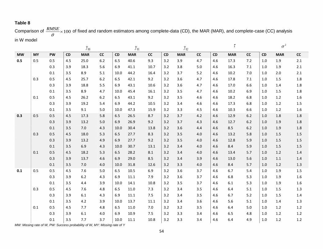
54
Table 8
Comparison of 100RMSE
of fixed and random estimators among complete-data (CD), the MAR (MAR), and complete-case (CC) analysis
in W model
00 01 02 2
MW MY PW CD MAR CC CD MAR CC CD MAR CC CD MAR CC CD MAR CC
0.5 0.5 0.5 4.5 25.0 6.2 6.5 40.6 9.3 3.2 3.9 4.7 4.6 17.3 7.2 1.0 1.9 2.1
0.3 3.9 18.3 5.6 6.9 41.1 10.7 3.2 3.8 5.0 4.6 16.3 7.1 1.0 1.9 2.1
0.1 3.5 8.9 5.1 10.0 44.2 16.4 3.2 3.7 5.2 4.6 10.2 7.0 1.0 2.0 2.1
0.3 0.5 4.5 25.7 6.2 6.5 42.1 9.2 3.2 3.6 4.7 4.6 17.8 7.1 1.0 1.5 1.8
0.3 3.9 18.8 5.5 6.9 43.1 10.6 3.2 3.6 4.7 4.6 17.0 6.6 1.0 1.4 1.8
0.1 3.5 8.9 4.7 10.0 45.4 16.1 3.2 3.5 4.7 4.6 10.2 6.9 1.0 1.5 1.8
0.1 0.5 4.5 26.2 6.2 6.5 43.1 9.2 3.2 3.5 4.6 4.6 18.2 6.8 1.0 1.2 1.6
0.3 3.9 19.2 5.4 6.9 44.2 10.5 3.2 3.4 4.6 4.6 17.3 6.8 1.0 1.2 1.5
0.1 3.5 9.1 5.0 10.0 47.3 15.9 3.2 3.3 4.5 4.6 10.3 6.6 1.0 1.2 1.6
0.3 0.5 0.5 4.5 17.3 5.8 6.5 26.5 8.7 3.2 3.7 4.2 4.6 12.9 6.2 1.0 1.8 1.8
0.3 3.9 13.2 5.0 6.9 26.9 9.2 3.2 3.7 4.3 4.6 12.7 6.2 1.0 1.9 1.8
0.1 3.5 7.0 4.3 10.0 30.4 13.8 3.2 3.6 4.4 4.6 8.5 6.2 1.0 1.9 1.8
0.3 0.5 4.5 18.0 5.3 6.5 27.7 8.3 3.2 3.5 4.0 4.6 13.2 5.8 1.0 1.5 1.5
0.3 3.9 13.2 4.9 6.9 27.7 9.2 3.2 3.5 4.0 4.6 12.8 5.9 1.0 1.5 1.5
0.1 3.5 6.9 4.3 10.0 30.7 13.1 3.2 3.4 4.0 4.6 8.4 5.9 1.0 1.5 1.5
0.1 0.5 4.5 18.2 5.3 6.5 28.2 8.1 3.2 3.4 4.0 4.6 13.4 5.7 1.0 1.2 1.4
0.3 3.9 13.7 4.6 6.9 29.0 8.5 3.2 3.4 3.9 4.6 13.0 5.6 1.0 1.1 1.4
0.1 3.5 7.0 4.0 10.0 31.8 12.6 3.2 3.3 4.0 4.6 8.4 5.7 1.0 1.2 1.3
0.1 0.5 0.5 4.5 7.6 5.0 6.5 10.5 6.9 3.2 3.6 3.7 4.6 6.7 5.4 1.0 1.9 1.5
0.3 3.9 6.2 4.3 6.9 11.1 7.9 3.2 3.6 3.7 4.6 6.8 5.3 1.0 1.9 1.6
0.1 3.5 4.4 3.9 10.0 14.1 10.8 3.2 3.5 3.7 4.6 6.1 5.3 1.0 1.9 1.6
0.3 0.5 4.5 7.6 4.8 6.5 11.0 7.3 3.2 3.4 3.5 4.6 6.4 5.1 1.0 1.5 1.3
0.3 3.9 6.1 4.3 6.9 11.1 7.5 3.2 3.4 3.5 4.6 6.7 5.2 1.0 1.5 1.4
0.1 3.5 4.2 3.9 10.0 13.7 11.1 3.2 3.4 3.6 4.6 5.6 5.1 1.0 1.4 1.3
0.1 0.5 4.5 7.7 4.8 6.5 11.0 7.0 3.2 3.2 3.5 4.6 6.4 5.0 1.0 1.2 1.2
0.3 3.9 6.1 4.0 6.9 10.9 7.5 3.2 3.3 3.4 4.6 6.5 4.8 1.0 1.2 1.2
0.1 3.5 7.7 3.7 10.0 11.1 10.8 3.2 3.3 3.4 4.6 6.4 4.9 1.0 1.2 1.2
MW: Missing rate of W, PW: Success probability of W, MY: Missing rate of Y

55
Table 9
Comparison of . 100S E of fixed and random estimators among complete-data (CD), the MAR (MAR), and complete-case (CC) analysis
in W model
00 01 02
2
MW MY PW CD MAR CC CD MAR CC CD MAR CC CD MAR CC CD MAR CC
0.5 0.5 0.5 4.6 1.3 6.3 6.5 2.2 9.7 3.2 0.9 4.9 4.7 1.4 7.1 1.0 0.3 2.1
0.3 4.0 4.8 5.6 6.9 11.0 10.9 3.2 3.8 5.0 4.7 6.0 7.2 1.0 1.5 2.1
0.1 3.5 3.9 5.0 9.6 15.7 16.6 3.2 3.7 5.0 4.7 5.7 7.2 1.0 1.5 2.1
0.3 0.5 4.6 5.6 6.1 6.5 9.7 9.4 3.2 3.7 4.7 4.7 5.9 6.8 1.0 1.3 1.8
0.3 4.0 4.7 5.4 6.9 10.9 10.6 3.2 3.7 4.7 4.7 5.8 6.8 1.0 1.3 1.8
0.1 3.5 3.8 4.9 9.6 15.7 16.1 3.2 3.6 4.7 4.7 5.4 6.8 1.0 1.3 1.8
0.1 0.5 4.6 5.6 6.0 6.5 9.6 9.2 3.2 3.6 4.6 4.7 5.7 6.6 1.0 1.1 1.6
0.3 4.0 3.8 5.3 6.9 15.7 10.4 3.2 3.6 4.6 4.7 5.4 6.6 1.0 1.3 1.6
0.1 3.5 3.8 4.8 9.6 15.7 15.8 3.2 3.6 4.6 4.7 5.4 6.6 1.0 1.3 1.6
0.3 0.5 0.5 4.6 5.5 5.6 6.5 8.9 8.4 3.2 3.8 4.3 4.7 5.9 6.2 1.0 1.5 1.8
0.3 4.0 4.7 4.9 6.9 9.7 9.3 3.2 3.8 4.3 4.7 5.9 6.2 1.0 1.5 1.8
0.1 3.5 3.9 4.4 9.6 14.0 13.7 3.2 3.7 4.3 4.7 5.6 6.2 1.0 1.5 1.8
0.3 0.5 4.6 5.5 5.4 6.5 8.8 8.1 3.2 3.6 4.1 4.7 5.7 5.9 1.0 1.3 1.6
0.3 4.0 4.6 4.8 6.9 9.6 9.0 3.2 3.6 4.1 4.7 5.6 5.9 1.0 1.3 1.6
0.1 3.5 3.8 4.3 9.6 13.7 13.3 3.2 3.5 4.1 4.7 5.3 5.9 1.0 1.3 1.6
0.1 0.5 4.6 5.4 5.3 6.5 8.7 8.0 3.2 3.5 4.0 4.7 5.5 5.8 1.0 1.1 1.4
0.3 4.0 4.5 5.3 6.9 9.5 8.0 3.2 3.5 4.0 4.7 5.5 5.8 1.0 1.1 1.4
0.1 3.5 3.7 4.7 9.6 13.6 8.8 3.2 3.4 4.0 4.7 5.1 5.8 1.0 1.1 1.4
0.1 0.5 0.5 4.6 5.2 5.0 6.5 7.6 7.3 3.2 3.7 3.8 4.7 5.5 5.4 1.0 1.5 1.6
0.3 4.0 4.4 4.4 6.9 8.2 7.8 3.2 3.7 3.8 4.7 5.5 5.4 1.0 1.5 1.6
0.1 3.5 3.8 3.9 9.6 11.5 11.1 3.2 3.6 3.8 4.7 5.4 5.4 1.0 1.5 1.6
0.3 0.5 4.6 5.0 4.9 6.5 7.4 7.0 3.2 3.5 3.6 4.7 5.2 5.2 1.0 1.3 1.4
0.3 4.0 4.3 4.3 6.9 8.0 7.6 3.2 3.5 3.6 4.7 5.2 5.2 1.0 1.3 1.4
0.1 3.5 3.7 3.8 9.6 11.1 10.8 3.2 3.5 3.6 4.7 5.1 5.2 1.0 1.3 1.4
0.1 0.5 4.6 4.9 4.8 6.5 7.3 6.9 3.2 3.4 3.5 4.7 5.1 5.0 1.0 1.1 1.2
0.3 4.0 4.2 4.2 6.9 7.8 7.4 3.2 3.4 3.5 4.7 5.1 5.0 1.0 1.1 1.2
0.1 3.5 4.9 3.7 9.6 7.3 10.6 3.2 3.4 3.5 4.7 5.1 5.0 1.0 1.1 1.2
MW: Missing rate of W, PW: Success probability of W, MY: Missing rate of Y
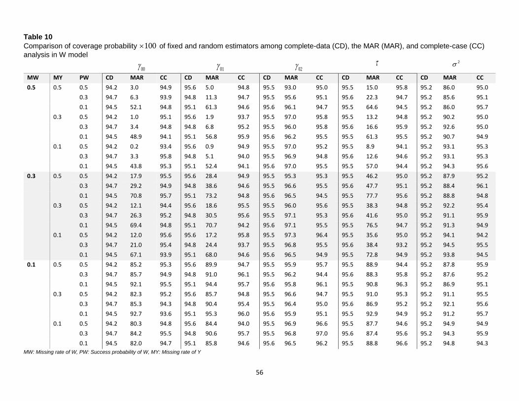
56
Table 10
Comparison of coverage probability 100 of fixed and random estimators among complete-data (CD), the MAR (MAR), and complete-case (CC)
analysis in W model
00 01 02 2
MW MY PW CD MAR CC CD MAR CC CD MAR CC CD MAR CC CD MAR CC
0.5 0.5 0.5 94.2 3.0 94.9 95.6 5.0 94.8 95.5 93.0 95.0 95.5 15.0 95.8 95.2 86.0 95.0
0.3 94.7 6.3 93.9 94.8 11.3 94.7 95.5 95.6 95.1 95.6 22.3 94.7 95.2 85.6 95.1
0.1 94.5 52.1 94.8 95.1 61.3 94.6 95.6 96.1 94.7 95.5 64.6 94.5 95.2 86.0 95.7
0.3 0.5 94.2 1.0 95.1 95.6 1.9 93.7 95.5 97.0 95.8 95.5 13.2 94.8 95.2 90.2 95.0
0.3 94.7 3.4 94.8 94.8 6.8 95.2 95.5 96.0 95.8 95.6 16.6 95.9 95.2 92.6 95.0
0.1 94.5 48.9 94.1 95.1 56.8 95.9 95.6 96.2 95.5 95.5 61.3 95.5 95.2 90.7 94.9
0.1 0.5 94.2 0.2 93.4 95.6 0.9 94.9 95.5 97.0 95.2 95.5 8.9 94.1 95.2 93.1 95.3
0.3 94.7 3.3 95.8 94.8 5.1 94.0 95.5 96.9 94.8 95.6 12.6 94.6 95.2 93.1 95.3
0.1 94.5 43.8 95.3 95.1 52.4 94.1 95.6 97.0 95.5 95.5 57.0 94.4 95.2 94.3 95.6
0.3 0.5 0.5 94.2 17.9 95.5 95.6 28.4 94.9 95.5 95.3 95.3 95.5 46.2 95.0 95.2 87.9 95.2
0.3 94.7 29.2 94.9 94.8 38.6 94.6 95.5 96.6 95.5 95.6 47.7 95.1 95.2 88.4 96.1
0.1 94.5 70.8 95.7 95.1 73.2 94.8 95.6 96.5 94.5 95.5 77.7 95.6 95.2 88.8 94.8
0.3 0.5 94.2 12.1 94.4 95.6 18.6 95.5 95.5 96.0 95.6 95.5 38.3 94.8 95.2 92.2 95.4
0.3 94.7 26.3 95.2 94.8 30.5 95.6 95.5 97.1 95.3 95.6 41.6 95.0 95.2 91.1 95.9
0.1 94.5 69.4 94.8 95.1 70.7 94.2 95.6 97.1 95.5 95.5 76.5 94.7 95.2 91.3 94.9
0.1 0.5 94.2 12.0 95.6 95.6 17.2 95.8 95.5 97.3 96.4 95.5 35.6 95.0 95.2 94.1 94.2
0.3 94.7 21.0 95.4 94.8 24.4 93.7 95.5 96.8 95.5 95.6 38.4 93.2 95.2 94.5 95.5
0.1 94.5 67.1 93.9 95.1 68.0 94.6 95.6 96.5 94.9 95.5 72.8 94.9 95.2 93.8 94.5
0.1 0.5 0.5 94.2 85.2 95.3 95.6 89.9 94.7 95.5 95.9 95.7 95.5 88.9 94.4 95.2 87.8 95.9
0.3 94.7 85.7 94.9 94.8 91.0 96.1 95.5 96.2 94.4 95.6 88.3 95.8 95.2 87.6 95.2
0.1 94.5 92.1 95.5 95.1 94.4 95.7 95.6 95.8 96.1 95.5 90.8 96.3 95.2 86.9 95.1
0.3 0.5 94.2 82.3 95.2 95.6 85.7 94.8 95.5 96.6 94.7 95.5 91.0 95.3 95.2 91.1 95.5
0.3 94.7 85.3 94.3 94.8 90.4 95.4 95.5 96.4 95.0 95.6 86.9 95.2 95.2 92.1 95.6
0.1 94.5 92.7 93.6 95.1 95.3 96.0 95.6 95.9 95.1 95.5 92.9 94.9 95.2 91.2 95.7
0.1 0.5 94.2 80.3 94.8 95.6 84.4 94.0 95.5 96.9 96.6 95.5 87.7 94.6 95.2 94.9 94.9
0.3 94.7 84.2 95.5 94.8 90.6 95.7 95.5 96.8 97.0 95.6 87.4 95.6 95.2 94.3 95.9
0.1 94.5 82.0 94.7 95.1 85.8 94.6 95.6 96.5 96.2 95.5 88.8 96.6 95.2 94.8 94.3
MW: Missing rate of W, PW: Success probability of W, MY: Missing rate of Y

57
Table 11
Comparison of 100Bias
of fixed and random estimators among complete-data (CD), the MAR (MAR), and complete-case (CC) analysis in
X and W model
00
01
02
10
20 2
MW MY MX PW PX CD MAR CC CD MAR CC CD MAR CC CD MAR CC CD MAR CC CD MAR CC CD MAR CC
0.1 0.2 0.1 0.1 0.1 0.0 2.5 0.0 0.2 -9.4 -0.4 -0.2 -0.2 -0.2 0.1 0.0 -0.1 0.0 0.4 0.0 -0.4 2.5 -0.5 0.0 0.4 0.0
0.5 0.0 2.5 0.1 0.0 -9.9 -0.6 -0.2 -0.2 -0.2 -0.1 -0.3 0.0 0.0 0.0 0.0 -0.4 2.5 -0.4 0.0 0.1 0.0
0.5 0.1 0.2 6.1 0.2 -0.4 -8.4 -0.4 -0.2 -0.2 -0.2 0.0 0.0 -0.1 0.0 0.4 0.0 -0.4 4.1 -0.5 0.0 0.5 0.0
0.5 0.0 6.0 0.4 -0.1 -8.4 -0.6 -0.2 -0.2 -0.2 0.0 0.0 -0.1 0.0 0.4 0.0 -0.4 4.1 -0.4 0.0 0.5 0.0
0.3 0.1 0.1 0.0 2.8 0.0 0.2 -9.8 0.0 -0.2 -0.1 -0.2 0.1 0.1 0.0 0.0 1.2 -0.1 -0.4 2.4 -0.5 0.0 1.4 -0.1
0.5 0.0 2.7 0.1 0.0 -9.4 -0.1 -0.2 -0.2 -0.1 -0.1 -0.8 -0.2 0.0 0.0 0.0 -0.4 2.3 -0.4 0.0 0.2 0.0
0.5 0.1 0.2 6.5 0.0 -0.4 -8.7 -0.1 -0.2 -0.2 -0.3 0.0 0.3 -0.1 0.0 1.2 0.0 -0.4 3.9 -0.3 0.0 1.4 0.0
0.5 0.0 6.6 0.3 -0.1 -8.7 -0.6 -0.2 -0.2 -0.2 0.0 -0.8 0.1 0.0 0.1 0.0 -0.4 4.9 -0.5 0.0 1.6 0.0
0.4 0.1 0.1 0.1 0.0 2.4 0.0 0.2 -8.9 0.0 -0.2 -0.2 -0.2 0.1 0.2 -0.1 0.0 0.5 0.0 -0.4 2.4 -0.5 0.0 0.6 0.0
0.5 0.0 2.3 0.0 0.0 -8.6 -0.5 -0.2 -0.2 -0.2 -0.1 -0.2 0.1 0.0 0.0 0.0 -0.4 2.5 -0.4 0.0 0.3 0.0
0.5 0.1 0.2 6.2 0.0 -0.4 -8.7 -0.2 -0.2 -0.2 -0.2 0.0 -0.2 0.2 0.0 0.4 0.0 -0.4 4.0 -0.6 0.0 0.5 0.0
0.5 0.0 6.2 0.1 -0.1 -8.4 -0.1 -0.2 -0.2 -0.2 0.0 -0.6 -0.1 0.0 0.0 0.0 -0.4 3.9 -0.4 0.0 0.4 0.0
0.3 0.1 0.1 0.0 2.7 0.0 0.2 -9.4 0.6 -0.2 -0.2 -0.2 0.1 -0.2 -0.1 0.0 1.3 0.0 -0.4 2.2 -0.4 0.0 1.5 0.0
0.5 0.0 2.9 0.0 0.0 -8.8 0.0 -0.2 -0.2 -0.2 -0.1 -1.3 -0.1 0.0 0.2 -0.1 -0.4 2.1 -0.4 0.0 0.5 0.0
0.5 0.1 0.2 6.2 0.2 -0.4 -8.0 -0.2 -0.2 -0.3 -0.2 0.0 -0.2 -0.1 0.0 1.3 0.0 -0.4 3.7 -0.4 0.0 1.4 0.0
0.5 0.0 6.4 0.1 -0.1 -8.2 -0.3 -0.2 -0.2 -0.3 0.0 -1.1 -0.1 0.0 0.1 0.0 -0.4 3.5 -0.5 0.0 0.5 0.0
0.3 0.2 0.1 0.1 0.1 0.0 6.1 0.2 0.2 -29.9 -0.5 -0.2 -0.2 -0.2 0.1 0.1 -0.1 0.0 0.4 0.0 -0.4 6.6 -0.5 0.0 0.5 0.0
0.5 0.0 6.2 0.0 0.0 -30.1 0.3 -0.2 -0.2 -0.2 -0.1 -0.3 -0.1 0.0 0.0 0.0 -0.4 6.6 -0.6 0.0 0.1 0.0
0.5 0.1 0.2 17.7 0.0 -0.4 -27.3 0.0 -0.2 -0.2 -0.1 0.0 0.2 0.0 0.0 0.4 0.0 -0.4 12.1 -0.5 0.0 0.4 0.0
0.5 0.0 17.5 0.2 -0.1 -27.0 -0.4 -0.2 -0.2 -0.2 0.0 -0.3 0.0 0.0 0.0 0.0 -0.4 12.2 -0.4 0.0 0.2 0.0
0.3 0.1 0.1 0.0 6.5 0.0 0.2 -30.0 0.5 -0.2 -0.2 -0.1 0.1 0.3 0.1 0.0 1.2 -0.1 -0.4 6.6 -0.7 0.0 1.3 0.0
0.5 0.0 6.4 0.1 0.0 -30.1 0.0 -0.2 -0.2 -0.3 -0.1 -0.7 0.0 0.0 0.1 -0.1 -0.4 6.4 -0.6 0.0 0.3 0.0
0.5 0.1 0.2 18.0 0.0 -0.4 -27.5 0.1 -0.2 -0.2 -0.1 0.0 0.2 0.0 0.0 1.2 0.0 -0.4 12.1 -0.3 0.0 1.3 -0.1
0.5 0.0 17.9 0.0 -0.1 -27.5 0.0 -0.2 -0.4 -0.1 0.0 -1.0 0.0 0.0 0.0 0.0 -0.4 12.0 -0.7 0.0 0.2 -0.1
0.4 0.1 0.1 0.1 0.0 6.0 0.1 0.2 -28.3 -0.6 -0.2 -0.3 -0.2 0.1 0.0 0.1 0.0 0.4 -0.1 -0.4 6.4 -1.0 0.0 0.5 0.0
0.5 0.0 6.0 0.0 0.0 -28.5 -0.5 -0.2 -0.2 -0.1 -0.1 -0.3 0.1 0.0 0.0 0.0 -0.4 6.7 -0.7 0.0 0.4 -0.1
0.5 0.1 0.2 17.1 0.2 -0.4 -26.0 -0.4 -0.2 -0.3 -0.3 0.0 -0.1 -0.1 0.0 0.4 0.0 -0.4 11.8 -0.5 0.0 0.5 -0.1
0.5 0.0 17.1 0.0 -0.1 -26.0 0.1 -0.2 -0.3 -0.2 0.0 -0.6 0.0 0.0 0.1 0.0 -0.4 11.8 -0.7 0.0 0.3 0.0
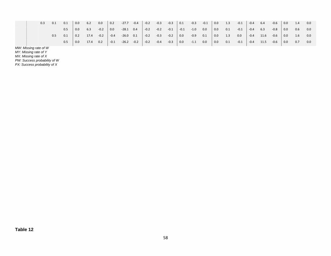
58
0.3 0.1 0.1 0.0 6.2 0.0 0.2 -27.7 -0.4 -0.2 -0.3 -0.3 0.1 -0.3 -0.1 0.0 1.3 -0.1 -0.4 6.4 -0.6 0.0 1.4 0.0
0.5 0.0 6.3 -0.2 0.0 -28.1 0.4 -0.2 -0.2 -0.1 -0.1 -1.0 0.0 0.0 0.1 -0.1 -0.4 6.3 -0.8 0.0 0.6 0.0
0.5 0.1 0.2 17.4 -0.2 -0.4 -26.0 0.1 -0.2 -0.3 -0.2 0.0 -0.9 0.1 0.0 1.3 0.0 -0.4 11.6 -0.6 0.0 1.6 0.0
0.5 0.0 17.4 0.2 -0.1 -26.2 -0.2 -0.2 -0.4 -0.3 0.0 -1.1 0.0 0.0 0.1 -0.1 -0.4 11.5 -0.6 0.0 0.7 0.0
MW: Missing rate of W
MY: Missing rate of Y
MX: Missing rate of X
PW: Success probability of W
PX: Success probability of X
Table 12
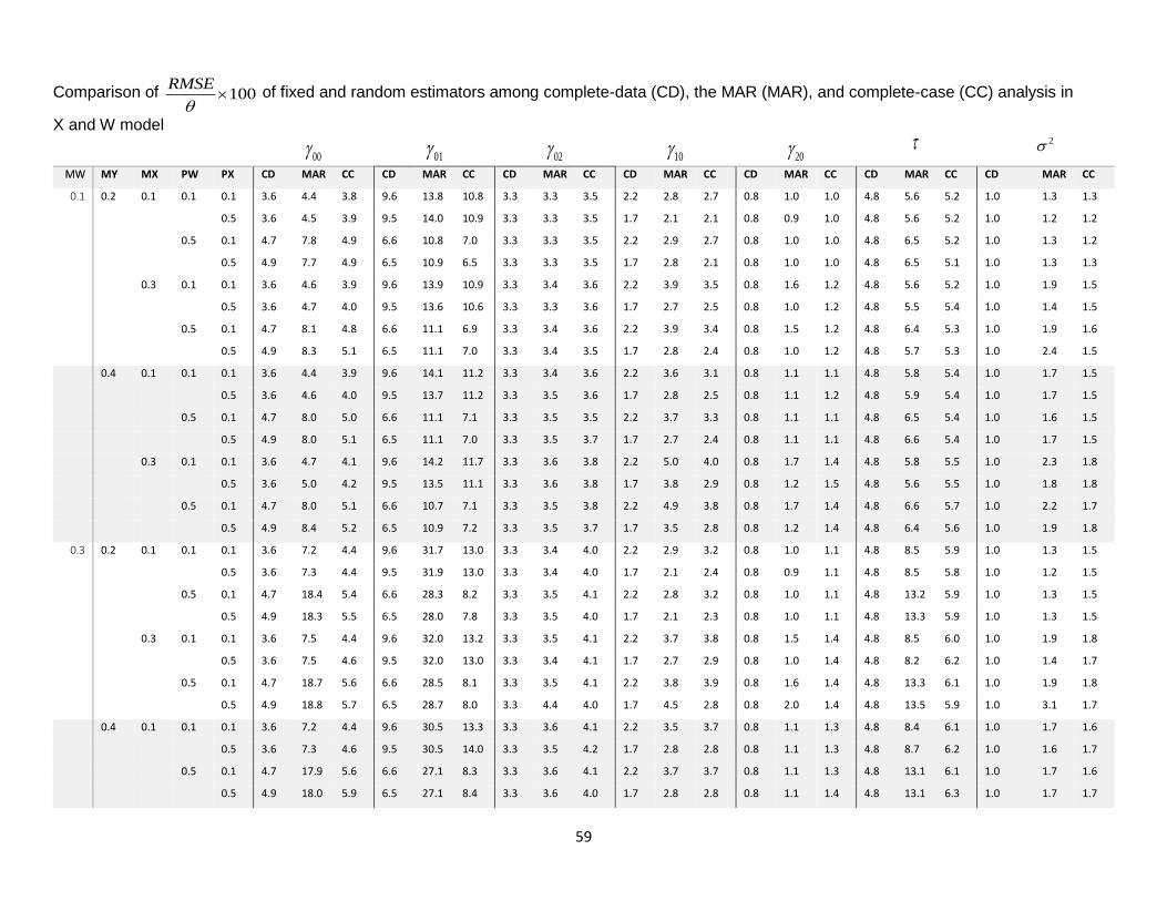
59
Comparison of 100RMSE
of fixed and random estimators among complete-data (CD), the MAR (MAR), and complete-case (CC) analysis in
X and W model
00 01 02 10 20
2
MW MY MX PW PX CD MAR CC CD MAR CC CD MAR CC CD MAR CC CD MAR CC CD MAR CC CD MAR CC
0.1 0.2 0.1 0.1 0.1 3.6 4.4 3.8 9.6 13.8 10.8 3.3 3.3 3.5 2.2 2.8 2.7 0.8 1.0 1.0 4.8 5.6 5.2 1.0 1.3 1.3
0.5 3.6 4.5 3.9 9.5 14.0 10.9 3.3 3.3 3.5 1.7 2.1 2.1 0.8 0.9 1.0 4.8 5.6 5.2 1.0 1.2 1.2
0.5 0.1 4.7 7.8 4.9 6.6 10.8 7.0 3.3 3.3 3.5 2.2 2.9 2.7 0.8 1.0 1.0 4.8 6.5 5.2 1.0 1.3 1.2
0.5 4.9 7.7 4.9 6.5 10.9 6.5 3.3 3.3 3.5 1.7 2.8 2.1 0.8 1.0 1.0 4.8 6.5 5.1 1.0 1.3 1.3
0.3 0.1 0.1 3.6 4.6 3.9 9.6 13.9 10.9 3.3 3.4 3.6 2.2 3.9 3.5 0.8 1.6 1.2 4.8 5.6 5.2 1.0 1.9 1.5
0.5 3.6 4.7 4.0 9.5 13.6 10.6 3.3 3.3 3.6 1.7 2.7 2.5 0.8 1.0 1.2 4.8 5.5 5.4 1.0 1.4 1.5
0.5 0.1 4.7 8.1 4.8 6.6 11.1 6.9 3.3 3.4 3.6 2.2 3.9 3.4 0.8 1.5 1.2 4.8 6.4 5.3 1.0 1.9 1.6
0.5 4.9 8.3 5.1 6.5 11.1 7.0 3.3 3.4 3.5 1.7 2.8 2.4 0.8 1.0 1.2 4.8 5.7 5.3 1.0 2.4 1.5
0.4 0.1 0.1 0.1 3.6 4.4 3.9 9.6 14.1 11.2 3.3 3.4 3.6 2.2 3.6 3.1 0.8 1.1 1.1 4.8 5.8 5.4 1.0 1.7 1.5
0.5 3.6 4.6 4.0 9.5 13.7 11.2 3.3 3.5 3.6 1.7 2.8 2.5 0.8 1.1 1.2 4.8 5.9 5.4 1.0 1.7 1.5
0.5 0.1 4.7 8.0 5.0 6.6 11.1 7.1 3.3 3.5 3.5 2.2 3.7 3.3 0.8 1.1 1.1 4.8 6.5 5.4 1.0 1.6 1.5
0.5 4.9 8.0 5.1 6.5 11.1 7.0 3.3 3.5 3.7 1.7 2.7 2.4 0.8 1.1 1.1 4.8 6.6 5.4 1.0 1.7 1.5
0.3 0.1 0.1 3.6 4.7 4.1 9.6 14.2 11.7 3.3 3.6 3.8 2.2 5.0 4.0 0.8 1.7 1.4 4.8 5.8 5.5 1.0 2.3 1.8
0.5 3.6 5.0 4.2 9.5 13.5 11.1 3.3 3.6 3.8 1.7 3.8 2.9 0.8 1.2 1.5 4.8 5.6 5.5 1.0 1.8 1.8
0.5 0.1 4.7 8.0 5.1 6.6 10.7 7.1 3.3 3.5 3.8 2.2 4.9 3.8 0.8 1.7 1.4 4.8 6.6 5.7 1.0 2.2 1.7
0.5 4.9 8.4 5.2 6.5 10.9 7.2 3.3 3.5 3.7 1.7 3.5 2.8 0.8 1.2 1.4 4.8 6.4 5.6 1.0 1.9 1.8
0.3 0.2 0.1 0.1 0.1 3.6 7.2 4.4 9.6 31.7 13.0 3.3 3.4 4.0 2.2 2.9 3.2 0.8 1.0 1.1 4.8 8.5 5.9 1.0 1.3 1.5
0.5 3.6 7.3 4.4 9.5 31.9 13.0 3.3 3.4 4.0 1.7 2.1 2.4 0.8 0.9 1.1 4.8 8.5 5.8 1.0 1.2 1.5
0.5 0.1 4.7 18.4 5.4 6.6 28.3 8.2 3.3 3.5 4.1 2.2 2.8 3.2 0.8 1.0 1.1 4.8 13.2 5.9 1.0 1.3 1.5
0.5 4.9 18.3 5.5 6.5 28.0 7.8 3.3 3.5 4.0 1.7 2.1 2.3 0.8 1.0 1.1 4.8 13.3 5.9 1.0 1.3 1.5
0.3 0.1 0.1 3.6 7.5 4.4 9.6 32.0 13.2 3.3 3.5 4.1 2.2 3.7 3.8 0.8 1.5 1.4 4.8 8.5 6.0 1.0 1.9 1.8
0.5 3.6 7.5 4.6 9.5 32.0 13.0 3.3 3.4 4.1 1.7 2.7 2.9 0.8 1.0 1.4 4.8 8.2 6.2 1.0 1.4 1.7
0.5 0.1 4.7 18.7 5.6 6.6 28.5 8.1 3.3 3.5 4.1 2.2 3.8 3.9 0.8 1.6 1.4 4.8 13.3 6.1 1.0 1.9 1.8
0.5 4.9 18.8 5.7 6.5 28.7 8.0 3.3 4.4 4.0 1.7 4.5 2.8 0.8 2.0 1.4 4.8 13.5 5.9 1.0 3.1 1.7
0.4 0.1 0.1 0.1 3.6 7.2 4.4 9.6 30.5 13.3 3.3 3.6 4.1 2.2 3.5 3.7 0.8 1.1 1.3 4.8 8.4 6.1 1.0 1.7 1.6
0.5 3.6 7.3 4.6 9.5 30.5 14.0 3.3 3.5 4.2 1.7 2.8 2.8 0.8 1.1 1.3 4.8 8.7 6.2 1.0 1.6 1.7
0.5 0.1 4.7 17.9 5.6 6.6 27.1 8.3 3.3 3.6 4.1 2.2 3.7 3.7 0.8 1.1 1.3 4.8 13.1 6.1 1.0 1.7 1.6
0.5 4.9 18.0 5.9 6.5 27.1 8.4 3.3 3.6 4.0 1.7 2.8 2.8 0.8 1.1 1.4 4.8 13.1 6.3 1.0 1.7 1.7

60
0.3 0.1 0.1 3.6 7.3 4.6 9.6 29.8 14.1 3.3 3.5 4.4 2.2 4.8 4.4 0.8 1.7 1.6 4.8 8.4 6.4 1.0 2.2 2.0
0.5 3.6 7.7 4.8 9.5 30.2 14.1 3.3 3.6 4.5 1.7 3.6 3.3 0.8 1.2 1.6 4.8 8.5 6.7 1.0 2.0 2.0
0.5 0.1 4.7 18.2 5.9 6.6 27.1 8.3 3.3 3.8 4.4 2.2 5.3 4.5 0.8 1.7 1.6 4.8 12.9 6.7 1.0 2.4 2.1
0.5 4.9 18.1 6.0 6.5 27.2 8.4 3.3 3.9 4.4 1.7 3.6 3.2 0.8 1.2 1.7 4.8 12.7 6.3 1.0 1.9 2.0
MW: Missing rate of W
MY: Missing rate of Y
MX: Missing rate of X
PW: Success probability of W
PX: Success probability of X
Table 13

61
Comparison of . 100S E of fixed and random estimators among complete-data (CD), the MAR (MAR), and complete-case (CC) analysis in
X and W model
00
01
02
10
20 2
MW MY MX PW PX CD MAR CC CD MAR CC CD MAR CC CD MAR CC CD MAR CC CD MAR CC CD MAR CC
0.1 0.2 0.1 0.1 0.1 3.5 3.6 3.7 9.6 11.0 10.7 3.2 3.4 3.5 2.2 2.6 2.7 0.8 0.9 1.0 4.7 5.0 5.1 1.0 1.2 1.3
0.5 3.6 3.7 3.8 9.6 11.0 10.7 3.2 3.4 3.5 1.7 2.0 2.1 0.8 0.9 1.0 4.7 5.0 5.1 1.0 1.2 1.3
0.5 0.1 4.6 4.9 4.8 6.5 7.3 6.9 3.2 3.4 3.5 2.2 2.6 2.7 0.8 0.9 1.0 4.7 5.1 5.1 1.0 1.2 1.3
0.5 4.7 4.9 4.9 6.5 7.3 6.9 3.2 3.4 3.5 1.7 2.6 2.1 0.8 0.9 1.0 4.7 5.1 5.1 1.0 1.2 1.3
0.3 0.1 0.1 3.5 3.6 3.8 9.6 11.0 10.9 3.2 3.4 3.6 2.2 3.2 3.4 0.8 0.9 1.2 4.7 5.0 5.2 1.0 1.2 1.5
0.5 3.6 3.8 4.0 9.6 11.0 10.8 3.2 3.4 3.6 1.7 2.3 2.5 0.8 1.0 1.2 4.7 5.0 5.3 1.0 1.3 1.5
0.5 0.1 4.6 5.0 4.9 6.5 7.3 7.1 3.2 3.4 3.6 2.2 3.2 3.4 0.8 0.9 1.2 4.7 5.1 5.2 1.0 1.2 1.5
0.5 4.7 5.1 5.1 6.5 7.3 7.1 3.2 3.4 3.6 1.7 2.3 2.5 0.8 1.0 1.2 4.7 5.1 5.2 1.0 1.3 1.5
0.4 0.1 0.1 0.1 3.5 3.7 5.0 9.6 11.2 7.1 3.2 3.5 3.7 2.2 3.1 3.2 0.8 1.0 1.1 4.7 5.2 5.3 1.0 1.4 1.5
0.5 3.6 3.9 4.0 9.6 11.2 10.9 3.2 3.5 3.7 1.7 2.3 2.4 0.8 1.1 1.2 4.7 5.2 5.3 1.0 1.4 1.5
0.5 0.1 4.6 5.1 5.0 6.5 7.5 7.1 3.2 3.6 3.7 2.2 3.1 3.2 0.8 1.0 1.1 4.7 5.3 5.3 1.0 1.4 1.5
0.5 4.7 5.2 5.1 6.5 7.5 7.1 3.2 3.6 3.7 1.7 2.3 2.4 0.8 1.1 1.2 4.7 5.3 5.3 1.0 1.4 1.5
0.3 0.1 0.1 3.5 3.8 4.0 9.6 11.2 11.2 3.2 3.5 3.8 2.2 3.7 4.0 0.8 1.1 1.4 4.7 5.2 5.6 1.0 1.4 1.8
0.5 3.6 3.9 4.2 9.6 11.2 11.3 3.2 3.5 3.8 1.7 2.7 2.9 0.8 1.1 1.4 4.7 5.2 5.6 1.0 1.5 1.8
0.5 0.1 4.6 5.1 5.3 6.5 7.5 7.3 3.2 3.6 3.8 2.2 3.7 2.9 0.8 1.1 1.4 4.7 5.3 5.6 1.0 1.5 1.8
0.5 4.7 5.2 5.2 6.5 7.5 7.3 3.2 3.6 3.8 1.7 2.6 4.0 0.8 1.1 1.4 4.7 5.3 5.6 1.0 1.5 1.8
0.3 0.2 0.1 0.1 0.1 3.5 3.7 4.2 9.6 13.6 13.2 3.2 3.4 4.0 2.2 2.6 3.1 0.8 0.9 1.1 4.7 5.2 5.8 1.0 1.2 1.5
0.5 3.6 3.8 4.4 9.6 13.6 13.1 3.2 3.4 4.0 1.7 2.0 2.4 0.8 0.9 1.1 4.7 5.2 5.8 1.0 1.2 1.5
0.5 0.1 4.6 5.4 5.4 6.5 8.7 8.0 3.2 3.5 4.0 2.2 2.6 3.1 0.8 0.9 1.1 4.7 5.5 5.8 1.0 1.2 1.5
0.5 4.7 5.5 5.5 6.5 8.7 8.0 3.2 3.5 4.0 1.7 2.0 2.4 0.8 0.9 1.1 4.7 5.5 5.8 1.0 1.2 1.5
0.3 0.1 0.1 3.5 3.7 4.3 9.6 13.5 13.4 3.2 3.4 4.1 2.2 3.2 3.9 0.8 0.9 1.4 4.7 5.2 6.0 1.0 1.2 1.7
0.5 3.6 3.9 4.5 9.6 13.6 13.3 3.2 3.4 4.1 1.7 2.3 2.8 0.8 1.0 1.4 4.7 5.2 6.0 1.0 1.3 1.7
0.5 0.1 4.6 5.4 5.5 6.5 8.7 8.2 3.2 3.6 4.1 2.2 3.2 3.9 0.8 0.9 1.4 4.7 5.6 6.0 1.0 1.2 1.7
0.5 4.7 5.5 5.6 6.5 8.7 8.2 3.2 3.5 4.1 1.7 2.2 2.8 0.8 1.0 1.4 4.7 5.6 6.0 1.0 1.2 1.7
0.4 0.1 0.1 0.1 3.5 3.8 4.4 9.6 13.7 13.5 3.2 3.6 4.2 2.2 3.1 3.7 0.8 1.0 1.3 4.7 5.4 6.1 1.0 1.4 1.7
0.5 3.6 4.0 4.5 9.6 13.8 13.5 3.2 3.6 4.2 1.7 2.4 2.8 0.8 1.1 1.3 4.7 5.4 6.1 1.0 1.4 1.7
0.5 0.1 4.6 5.5 5.5 6.5 8.8 8.2 3.2 3.7 4.2 2.2 3.1 3.7 0.8 1.0 1.3 4.7 5.7 6.1 1.0 1.4 1.7
0.5 4.7 5.6 5.7 6.5 8.8 8.2 3.2 3.7 4.2 1.7 2.3 2.8 0.8 1.1 1.3 4.7 5.7 6.1 1.0 1.4 1.7
0.3 0.1 0.1 3.5 3.9 4.5 9.6 13.7 13.9 3.2 3.6 4.4 2.2 3.7 4.6 0.8 1.1 1.6 4.7 5.4 6.4 1.0 1.5 2.0
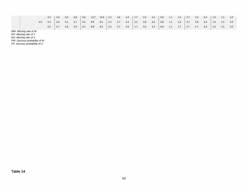
62
0.5 3.6 4.0 4.8 9.6 13.7 13.9 3.2 3.6 4.4 1.7 2.6 3.3 0.8 1.1 1.6 4.7 5.4 6.4 1.0 1.5 2.0
0.5 0.1 4.6 5.5 5.7 6.5 8.9 8.5 3.2 3.7 4.4 2.2 3.8 4.6 0.8 1.1 1.6 4.7 5.8 6.4 1.0 1.5 2.0
0.5 4.7 5.6 5.9 6.5 8.8 8.5 3.2 3.7 4.4 1.7 2.6 3.3 0.8 1.1 1.7 4.7 5.7 6.4 1.0 1.5 2.0
MW: Missing rate of W
MY: Missing rate of Y
MX: Missing rate of X
PW: Success probability of W
PX: Success probability of X
Table 14
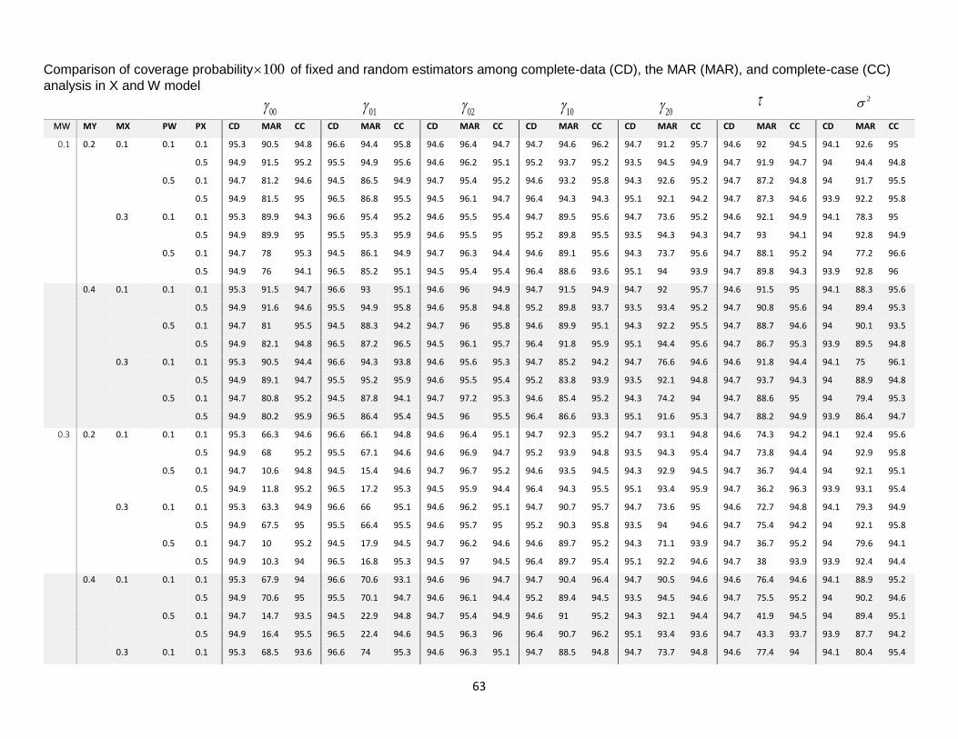
63
Comparison of coverage probability 100 of fixed and random estimators among complete-data (CD), the MAR (MAR), and complete-case (CC)
analysis in X and W model
00
01
02
10
20 2
MW MY MX PW PX CD MAR CC CD MAR CC CD MAR CC CD MAR CC CD MAR CC CD MAR CC CD MAR CC
0.1 0.2 0.1 0.1 0.1 95.3 90.5 94.8 96.6 94.4 95.8 94.6 96.4 94.7 94.7 94.6 96.2 94.7 91.2 95.7 94.6 92 94.5 94.1 92.6 95
0.5 94.9 91.5 95.2 95.5 94.9 95.6 94.6 96.2 95.1 95.2 93.7 95.2 93.5 94.5 94.9 94.7 91.9 94.7 94 94.4 94.8
0.5 0.1 94.7 81.2 94.6 94.5 86.5 94.9 94.7 95.4 95.2 94.6 93.2 95.8 94.3 92.6 95.2 94.7 87.2 94.8 94 91.7 95.5
0.5 94.9 81.5 95 96.5 86.8 95.5 94.5 96.1 94.7 96.4 94.3 94.3 95.1 92.1 94.2 94.7 87.3 94.6 93.9 92.2 95.8
0.3 0.1 0.1 95.3 89.9 94.3 96.6 95.4 95.2 94.6 95.5 95.4 94.7 89.5 95.6 94.7 73.6 95.2 94.6 92.1 94.9 94.1 78.3 95
0.5 94.9 89.9 95 95.5 95.3 95.9 94.6 95.5 95 95.2 89.8 95.5 93.5 94.3 94.3 94.7 93 94.1 94 92.8 94.9
0.5 0.1 94.7 78 95.3 94.5 86.1 94.9 94.7 96.3 94.4 94.6 89.1 95.6 94.3 73.7 95.6 94.7 88.1 95.2 94 77.2 96.6
0.5 94.9 76 94.1 96.5 85.2 95.1 94.5 95.4 95.4 96.4 88.6 93.6 95.1 94 93.9 94.7 89.8 94.3 93.9 92.8 96
0.4 0.1 0.1 0.1 95.3 91.5 94.7 96.6 93 95.1 94.6 96 94.9 94.7 91.5 94.9 94.7 92 95.7 94.6 91.5 95 94.1 88.3 95.6
0.5 94.9 91.6 94.6 95.5 94.9 95.8 94.6 95.8 94.8 95.2 89.8 93.7 93.5 93.4 95.2 94.7 90.8 95.6 94 89.4 95.3
0.5 0.1 94.7 81 95.5 94.5 88.3 94.2 94.7 96 95.8 94.6 89.9 95.1 94.3 92.2 95.5 94.7 88.7 94.6 94 90.1 93.5
0.5 94.9 82.1 94.8 96.5 87.2 96.5 94.5 96.1 95.7 96.4 91.8 95.9 95.1 94.4 95.6 94.7 86.7 95.3 93.9 89.5 94.8
0.3 0.1 0.1 95.3 90.5 94.4 96.6 94.3 93.8 94.6 95.6 95.3 94.7 85.2 94.2 94.7 76.6 94.6 94.6 91.8 94.4 94.1 75 96.1
0.5 94.9 89.1 94.7 95.5 95.2 95.9 94.6 95.5 95.4 95.2 83.8 93.9 93.5 92.1 94.8 94.7 93.7 94.3 94 88.9 94.8
0.5 0.1 94.7 80.8 95.2 94.5 87.8 94.1 94.7 97.2 95.3 94.6 85.4 95.2 94.3 74.2 94 94.7 88.6 95 94 79.4 95.3
0.5 94.9 80.2 95.9 96.5 86.4 95.4 94.5 96 95.5 96.4 86.6 93.3 95.1 91.6 95.3 94.7 88.2 94.9 93.9 86.4 94.7
0.3 0.2 0.1 0.1 0.1 95.3 66.3 94.6 96.6 66.1 94.8 94.6 96.4 95.1 94.7 92.3 95.2 94.7 93.1 94.8 94.6 74.3 94.2 94.1 92.4 95.6
0.5 94.9 68 95.2 95.5 67.1 94.6 94.6 96.9 94.7 95.2 93.9 94.8 93.5 94.3 95.4 94.7 73.8 94.4 94 92.9 95.8
0.5 0.1 94.7 10.6 94.8 94.5 15.4 94.6 94.7 96.7 95.2 94.6 93.5 94.5 94.3 92.9 94.5 94.7 36.7 94.4 94 92.1 95.1
0.5 94.9 11.8 95.2 96.5 17.2 95.3 94.5 95.9 94.4 96.4 94.3 95.5 95.1 93.4 95.9 94.7 36.2 96.3 93.9 93.1 95.4
0.3 0.1 0.1 95.3 63.3 94.9 96.6 66 95.1 94.6 96.2 95.1 94.7 90.7 95.7 94.7 73.6 95 94.6 72.7 94.8 94.1 79.3 94.9
0.5 94.9 67.5 95 95.5 66.4 95.5 94.6 95.7 95 95.2 90.3 95.8 93.5 94 94.6 94.7 75.4 94.2 94 92.1 95.8
0.5 0.1 94.7 10 95.2 94.5 17.9 94.5 94.7 96.2 94.6 94.6 89.7 95.2 94.3 71.1 93.9 94.7 36.7 95.2 94 79.6 94.1
0.5 94.9 10.3 94 96.5 16.8 95.3 94.5 97 94.5 96.4 89.7 95.4 95.1 92.2 94.6 94.7 38 93.9 93.9 92.4 94.4
0.4 0.1 0.1 0.1 95.3 67.9 94 96.6 70.6 93.1 94.6 96 94.7 94.7 90.4 96.4 94.7 90.5 94.6 94.6 76.4 94.6 94.1 88.9 95.2
0.5 94.9 70.6 95 95.5 70.1 94.7 94.6 96.1 94.4 95.2 89.4 94.5 93.5 94.5 94.6 94.7 75.5 95.2 94 90.2 94.6
0.5 0.1 94.7 14.7 93.5 94.5 22.9 94.8 94.7 95.4 94.9 94.6 91 95.2 94.3 92.1 94.4 94.7 41.9 94.5 94 89.4 95.1
0.5 94.9 16.4 95.5 96.5 22.4 94.6 94.5 96.3 96 96.4 90.7 96.2 95.1 93.4 93.6 94.7 43.3 93.7 93.9 87.7 94.2
0.3 0.1 0.1 95.3 68.5 93.6 96.6 74 95.3 94.6 96.3 95.1 94.7 88.5 94.8 94.7 73.7 94.8 94.6 77.4 94 94.1 80.4 95.4
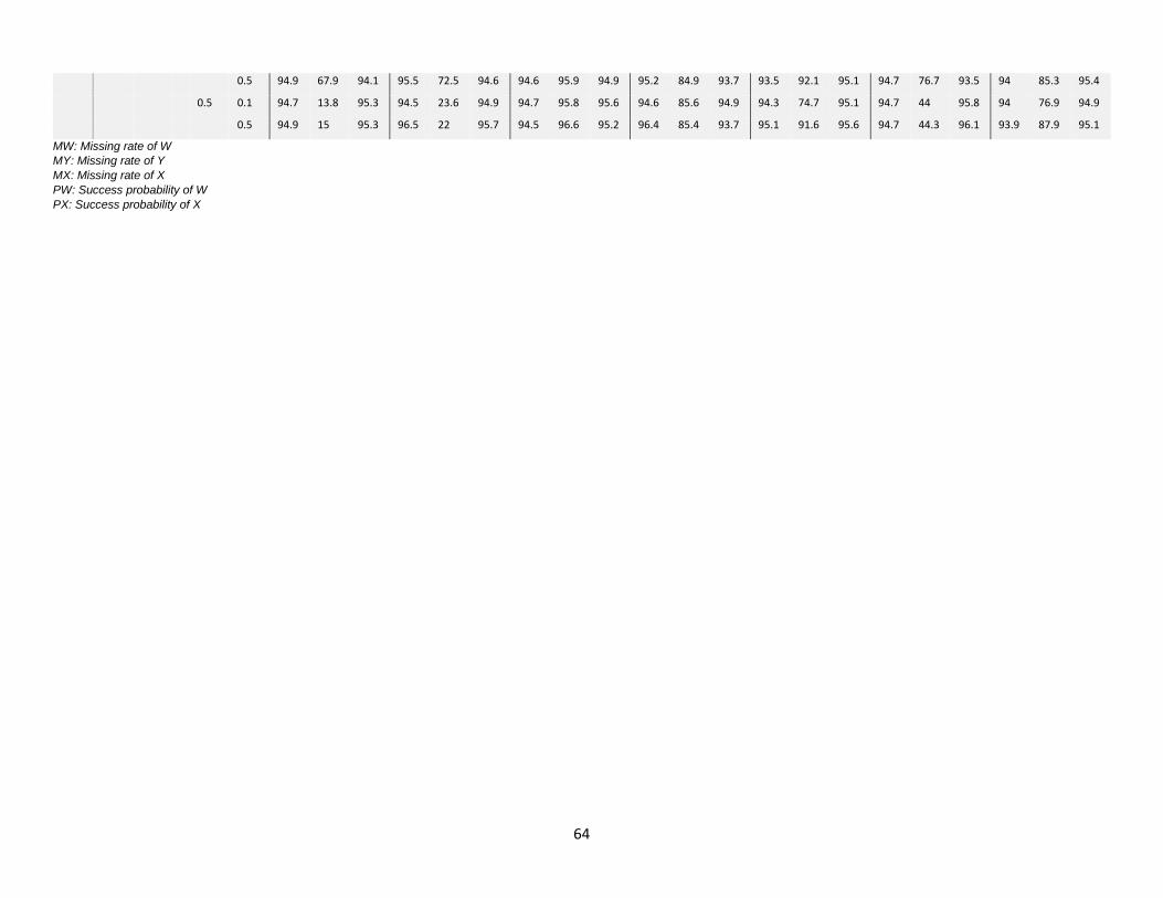
64
0.5 94.9 67.9 94.1 95.5 72.5 94.6 94.6 95.9 94.9 95.2 84.9 93.7 93.5 92.1 95.1 94.7 76.7 93.5 94 85.3 95.4
0.5 0.1 94.7 13.8 95.3 94.5 23.6 94.9 94.7 95.8 95.6 94.6 85.6 94.9 94.3 74.7 95.1 94.7 44 95.8 94 76.9 94.9
0.5 94.9 15 95.3 96.5 22 95.7 94.5 96.6 95.2 96.4 85.4 93.7 95.1 91.6 95.6 94.7 44.3 96.1 93.9 87.9 95.1
MW: Missing rate of W
MY: Missing rate of Y
MX: Missing rate of X
PW: Success probability of W
PX: Success probability of X

65
References [1] Little, R. J. A. & Rubin, D. B. (1987). Statistical analysis with missing data. New York: John Wiley & Sons.
[2] Shin, Y., & Raudenbush, S. W. (2007). Just‐Identified Versus Overidentified Two‐Level Hierarchical Linear
Models with Missing Data. Biometrics, 63(4), 1262-1268.
[3] Mark Fichman, Jonathon N. Cummings (2003). Multiple Imputation for Missing Data: Making the Most of
What you Know. Organizational Research Methods, 6, 3, 282-308.
[4] Allison, P. (2002). Missing data. Thousand Oaks, CA: Sage.
[5] Graham, J. W., Cumsille, P. E., & Elek-Fisk, E. (2003). Methods for handling missing data. In J. A. Schinka
& W. F. Velicer (Eds.). Research Methods in Psychology (pp. 87_114). Volume 2 of Handbook of Psychology
(I. B. Weiner, Editor-in-Chief). New York: John Wiley & Sons.
[6] Schafer, J. L., & Graham, J. W. (2002). Missing data: our view of the state of the art. Psychological
Methods, 7, 147-177.
[7] Rubin, D. B. (1976). Inference and missing data. Biometrika, 63(3), 581-592.
[8] Rubin, D. B. (1987). Multiple imputation for nonresponse in surveys (Vol. 81). John Wiley & Sons, New
York.
[9] Rubin, D. B. (1996). Multiple imputation after 18+ years. Journal of the American statistical
Association, 91(434), 473-489.
[10] Little, R. J., & Rubin, D. B. (2002). Single imputation methods. Statistical Analysis with Missing Data,
Second Edition, 59-74.
[11] Pigott, T. D. (2001). A review of methods for missing data. Educational research and evaluation, 7(4), 353-
383.
[12] Nakai M and Weiming Ke., 2011. Review of Methods for Handling Missing Data in Longitudinal Data
Analysis. Int. Journal of Math. Analysis. Vol. 5, no.1, 1-13.
[13] Little, R. J. A. & Rubin, D. B. (1989). The analysis of social science data with missing values. Sociological
methods and research, 18(2,3), 292-326.
[14] Shin, Y. (2013). Efficient Handling of Predictors and Outcomes Having Missing Values.
[15] Kropko, J., Goodrich, B., Gelman, A., & Hill, J. (2014). Multiple imputation for continuous and categorical
data: Comparing joint multivariate normal and conditional approaches. Political Analysis, mpu007.
[16] Rasbash, J., Steele, F., Browne, W. J., Goldstein, H. (2009). A user's guide to MLwiN Version
2.10. Centre for Multilevel Modelling, University of Bristol, UK.
[17] Raudenbush, S. W. Bryk, A.S., Cheong, Y., Congdon, R.T. and Mathilda du Toit (2011). HLM 7:
Hierarchical linear and nonlinear modeling. Scientific Software International.

66
[18] Lee, S. (2015). Implementing a Simulation Study Using Multiple Software Packages for Structural
Equation Modeling. SAGE Open, 5(3), 2158244015591823.
[19] Bauer, D. J., & Sterba, S. K. (2011). Fitting multilevel models with ordinal outcomes: Performance of
alternative specifications and methods of estimation. Psychological methods, 16(4), 373.
[20] Kaplan, D. (1989). A study of the sampling variability and z values of parameter estimates from
missspecificed structural equation models. Multivariate Behavioral Research, 24, 41-57. Doi:10.
1207/s15327906mbr2401-.
[21] Kendall, M. G., A. Stuart (1969). The Advanced Theory of Statistics. London, England: Griffin.
[22] Morrison JA (1992). Obesity and cardiovascular disease risk factors in black and white girls: the NHLBI
Growth and Health Study. American Journal of Public Health; 82: 1613-1620
[23] Graham, J. W., (2009). Missing data analysis: making it work in the real world. Annual Review of
Psychology, 60, 549-576.
[24] Graham, J. W., Taylor, B. J., Olchowski, A. E., & Cumsille, P. E. (2006). Planned missing data designs in
psychological research. Psychological Methods, 11, 323-343.
[25] Van Buuren, S. (2011). Multiple imputation of multilevel data. Handbook of advanced multilevel analysis,
173-196.
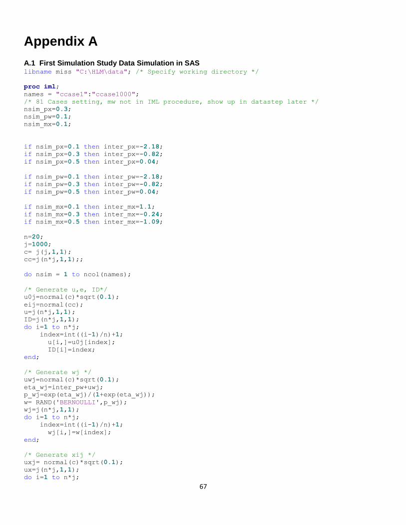
67
Appendix A
A.1 First Simulation Study Data Simulation in SAS libname miss "C:\HLM\data"; /* Specify working directory */
proc iml;
names = "ccase1":"ccase1000";
/* 81 Cases setting, mw not in IML procedure, show up in datastep later */
nsim_px=0.3;
nsim_pw=0.1;
nsim_mx=0.1;
if nsim_px=0.1 then inter_px=-2.18;
if nsim_px=0.3 then inter_px=-0.82;
if nsim_px=0.5 then inter_px=0.04;
if nsim_pw=0.1 then inter_pw=-2.18;
if nsim_pw=0.3 then inter_pw=-0.82;
if nsim_pw=0.5 then inter_pw=0.04;
if nsim_mx=0.1 then inter_mx=1.1;
if nsim_mx=0.3 then inter_mx=-0.24;
if nsim_mx=0.5 then inter_mx=-1.09;
n=20;
j=1000;
c= j(j,1,1);
cc=j(n*j,1,1);;
do nsim = 1 to ncol(names);
/* Generate u,e, ID*/
u0j=normal(c)*sqrt(0.1);
eij=normal(cc);
u=j(n*j,1,1);
ID=j(n*j,1,1);
do i=1 to n*j;
index=int((i-1)/n)+1;
u[i,]=u0j[index];
ID[i]=index;
end;
/* Generate wj */
uwj=normal(c)*sqrt(0.1);
eta_wj=inter_pw+uwj;
p_wj=exp(eta_wj)/(1+exp(eta_wj));
w= RAND('BERNOULLI',p_wj);
wj=j(n*j,1,1);
do i=1 to n*j;
index=int((i-1)/n)+1;
wj[i,]=w[index];
end;
/* Generate xij */
uxj= normal(c)*sqrt(0.1);
ux=j(n*j,1,1);
do i=1 to n*j;
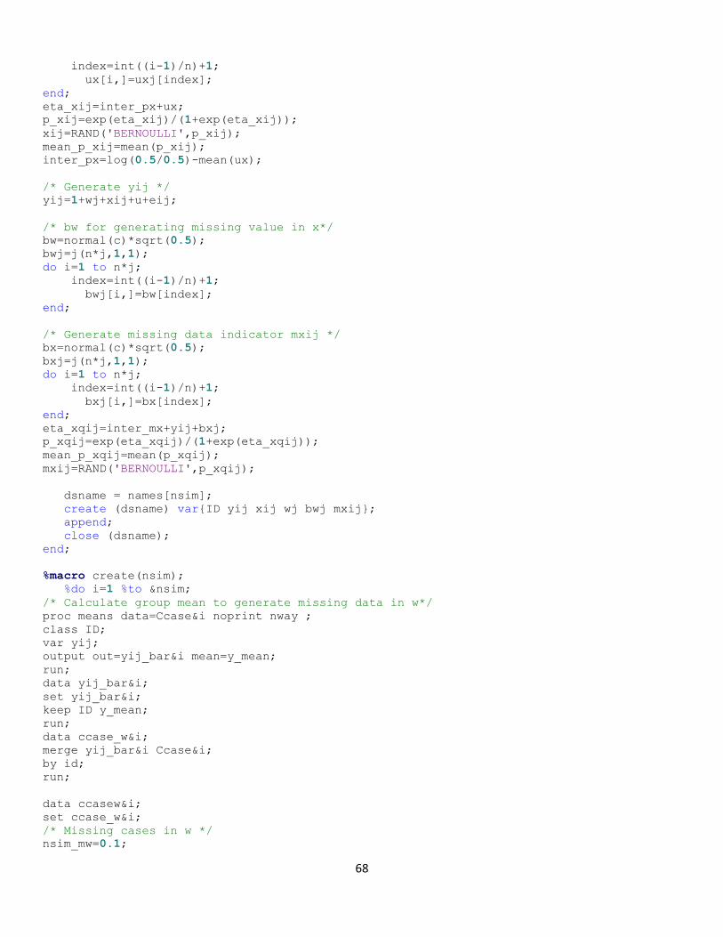
68
index=int((i-1)/n)+1;
ux[i,]=uxj[index];
end;
eta_xij=inter_px+ux;
p_xij=exp(eta_xij)/(1+exp(eta_xij));
xij=RAND('BERNOULLI',p_xij);
mean_p_xij=mean(p_xij);
inter_px=log(0.5/0.5)-mean(ux);
/* Generate yij */
yij=1+wj+xij+u+eij;
/* bw for generating missing value in x*/
bw=normal(c)*sqrt(0.5);
bwj=j(n*j,1,1);
do i=1 to n*j;
index=int((i-1)/n)+1;
bwj[i,]=bw[index];
end;
/* Generate missing data indicator mxij */
bx=normal(c)*sqrt(0.5);
bxj=j(n*j,1,1);
do i=1 to n*j;
index=int((i-1)/n)+1;
bxj[i,]=bx[index];
end;
eta_xqij=inter_mx+yij+bxj;
p_xqij=exp(eta_xqij)/(1+exp(eta_xqij));
mean_p_xqij=mean(p_xqij);
mxij=RAND('BERNOULLI',p_xqij);
dsname = names[nsim];
create (dsname) var{ID yij xij wj bwj mxij};
append;
close (dsname);
end;
%macro create(nsim);
%do i=1 %to ≁
/* Calculate group mean to generate missing data in w*/
proc means data=Ccase&i noprint nway ;
class ID;
var yij;
output out=yij_bar&i mean=y_mean;
run;
data yij_bar&i;
set yij_bar&i;
keep ID y_mean;
run;
data ccase_w&i;
merge yij_bar&i Ccase&i;
by id;
run;
data ccasew&i;
set ccase_w&i;
/* Missing cases in w */
nsim_mw=0.1;

69
if nsim_mw=0.1 then inter_mw=1.1;
if nsim_mw=0.3 then inter_mw=-0.24;
if nsim_mw=0.5 then inter_mw=-1.09;
eta_wqj=inter_mw+y_mean+bwj;
p_wqj=exp(eta_wqj)/(1+exp(eta_wqj));
run;
proc sort data=ccasew&i nodupkey;
by ID;
run;
data ccasew&i;
set ccasew&i;
mwj=RAND('BERNOULLI',p_wqj);
keep ID mwj;
run;
/* Create missing dataset rep1-rep1000*/
data miss.rep&i;
merge ccasew&i ccase_w&i;
by ID;
if mwj=0 then wj=.;
if mxij=0 then xij=.;
drop mwj bwj mxij y_mean;
run;
proc sort data=miss.rep&i;
by id;
run;
%end;
%mend create;
%create(1000)
A.2 Second Simulation Study Data Simulation in SAS
W Model Data Simulation in SAS libname w "C:\HLM\data";
proc iml;
names = "d1":"d1000";
nsim_mw=0.1;
nsim_my=0.1;
nsim_pw=0.5;
if nsim_mw=0.1 then inter_mw=2.5;
if nsim_mw=0.3 then inter_mw=0.9;
if nsim_mw=0.5 then inter_mw=0.07;
if nsim_my=0.1 then inter_my=2.2;
if nsim_my=0.3 then inter_my=0.9;
if nsim_my=0.5 then inter_my=0.02;
if nsim_pw=0.1 then inter_pw=-2.2;
if nsim_pw=0.3 then inter_pw=-0.82;
if nsim_pw=0.5 then inter_pw=0.003;
n=20;
j=1000;
c= j(j,1,1);
cc=j(n*j,1,1);
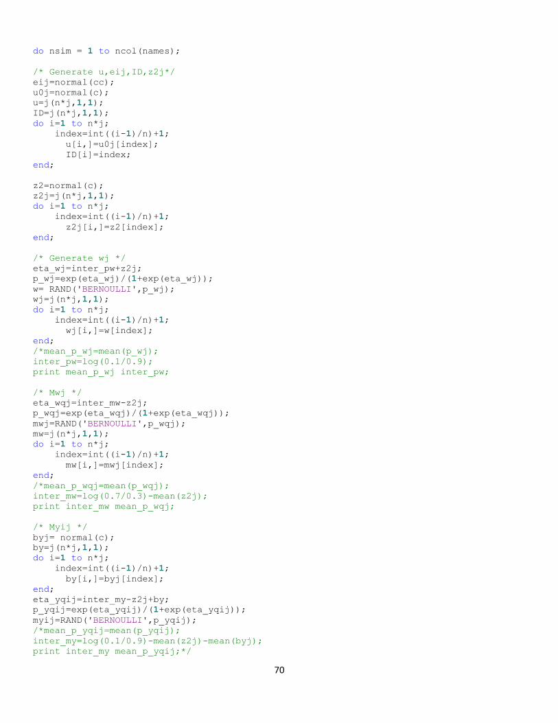
70
do nsim = 1 to ncol(names);
/* Generate u,eij,ID,z2j*/
eij=normal(cc);
u0j=normal(c);
u=j(n*j,1,1);
ID=j(n*j,1,1);
do i=1 to n*j;
index=int((i-1)/n)+1;
u[i,]=u0j[index];
ID[i]=index;
end;
z2=normal(c);
z2j=j(n*j,1,1);
do i=1 to n*j;
index=int((i-1)/n)+1;
z2j[i,]=z2[index];
end;
/* Generate wj */
eta_wj=inter_pw+z2j;
p_wj=exp(eta_wj)/(1+exp(eta_wj));
w= RAND('BERNOULLI',p_wj);
wj=j(n*j,1,1);
do i=1 to n*j;
index=int((i-1)/n)+1;
wj[i,]=w[index];
end;
/*mean_p_wj=mean(p_wj);
inter_pw=log(0.1/0.9);
print mean_p_wj inter_pw;
/* Mwj */
eta_wqj=inter_mw-z2j;
p_wqj=exp(eta_wqj)/(1+exp(eta_wqj));
mwj=RAND('BERNOULLI',p_wqj);
mw=j(n*j,1,1);
do i=1 to n*j;
index=int((i-1)/n)+1;
mw[i,]=mwj[index];
end;
/*mean_p_wqj=mean(p_wqj);
inter_mw=log(0.7/0.3)-mean(z2j);
print inter_mw mean_p_wqj;
/* Myij */
byj= normal(c);
by=j(n*j,1,1);
do i=1 to n*j;
index=int((i-1)/n)+1;
by[i,]=byj[index];
end;
eta_yqij=inter_my-z2j+by;
p_yqij=exp(eta_yqij)/(1+exp(eta_yqij));
myij=RAND('BERNOULLI',p_yqij);
/*mean_p_yqij=mean(p_yqij);
inter_my=log(0.1/0.9)-mean(z2j)-mean(byj);
print inter_my mean_p_yqij;*/
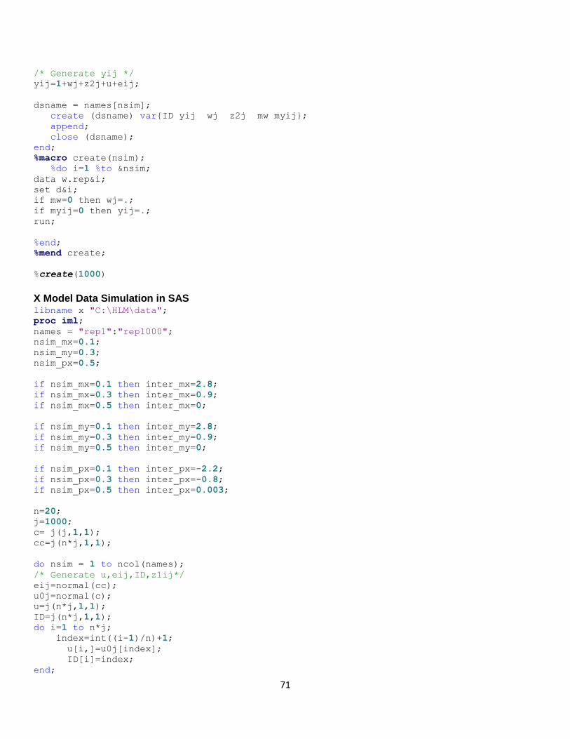
71
/* Generate yij */
yij=1+wj+z2j+u+eij;
dsname = names[nsim];
create (dsname) var{ID yij wj z2j mw myij};
append;
close (dsname);
end;
%macro create(nsim);
%do i=1 %to ≁
data w.rep&i;
set d&i;
if mw=0 then wj=.;
if myij=0 then yij=.;
run;
%end;
%mend create;
%create(1000)
X Model Data Simulation in SAS libname x "C:\HLM\data";
proc iml;
names = "rep1":"rep1000";
nsim_mx=0.1;
nsim_my=0.3;
nsim_px=0.5;
if nsim_mx=0.1 then inter_mx=2.8;
if nsim_mx=0.3 then inter_mx=0.9;
if nsim_mx=0.5 then inter_mx=0;
if nsim_my=0.1 then inter_my=2.8;
if nsim_my=0.3 then inter_my=0.9;
if nsim_my=0.5 then inter_my=0;
if nsim_px=0.1 then inter_px=-2.2;
if nsim_px=0.3 then inter_px=-0.8;
if nsim_px=0.5 then inter_px=0.003;
n=20;
j=1000;
c= j(j,1,1);
cc=j(n*j,1,1);
do nsim = 1 to ncol(names);
/* Generate u,eij,ID,z1ij*/
eij=normal(cc);
u0j=normal(c);
u=j(n*j,1,1);
ID=j(n*j,1,1);
do i=1 to n*j;
index=int((i-1)/n)+1;
u[i,]=u0j[index];
ID[i]=index;
end;

72
z1ij=normal(cc);
z2=normal(c);
z2j=j(n*j,1,1);
do i=1 to n*j;
index=int((i-1)/n)+1;
z2j[i,]=z2[index];
end;
/* Generate xij */
uxj= normal(c);
ux=j(n*j,1,1);
do i=1 to n*j;
index=int((i-1)/n)+1;
ux[i,]=uxj[index];
end;
eta_xij=inter_px+z1ij+ux;
p_xij=exp(eta_xij)/(1+exp(eta_xij));
xij=RAND('BERNOULLI',p_xij);
/*mean_p_xij=mean(p_xij);
inter_px=log(0.1/0.9)-mean(z1ij);
print mean_p_xij inter_px;*/
/* Generate yij */
yij=1+xij+z1ij+u+eij;
/* Mxij */
bxj= normal(c);
bx=j(n*j,1,1);
do i=1 to n*j;
index=int((i-1)/n)+1;
bx[i,]=bxj[index];
end;
eta_xqij=inter_mx-z1ij+bx;
p_xqij=exp(eta_xqij)/(1+exp(eta_xqij));
mxij=RAND('BERNOULLI',p_xqij);
/*mean_p_xqij=mean(p_xqij);
inter_mx=log(0.7/0.3)-mean(z1ij)-mean(bxj);
print inter_mx mean_p_xqij;*/
/* Myij */
byj= normal(c);
by=j(n*j,1,1);
do i=1 to n*j;
index=int((i-1)/n)+1;
by[i,]=byj[index];
end;
eta_yqij=inter_my-z1ij+by;
p_yqij=exp(eta_yqij)/(1+exp(eta_yqij));
myij=RAND('BERNOULLI',p_yqij);
/*mean_p_yqij=mean(p_yqij);
inter_my=log(0.1/0.9)-mean(z2j)-mean(byj);
print inter_my mean_p_yqij;*/
dsname = names[nsim];
create (dsname) var{ID yij xij z1ij z2j mxij myij};
append;
close (dsname);
end;

73
%macro create(nsim);
%do i=1 %to ≁
data x.rep&i;
set rep&i;
if mxij=0 then xij=.;
if myij=0 then yij=.;
run;
%end;
%mend create;
%create(1000)
W and X Model Data Simulation in SAS libname wx "C:\HLM\Data";
proc iml;
names = "rep1":"rep1000";
nsim_mw=0.3;
nsim_my=0.4;
nsim_mx=0.3;
nsim_pw=0.5;
nsim_px=0.5;
if nsim_mw=0.1 then inter_mw=2.5; else inter_mw=0.9;
if nsim_my=0.2 then inter_my=2; else inter_my=0.6;
if nsim_mx=0.1 then inter_mx=3; else inter_mx=0.9;
if nsim_pw=0.1 then inter_pw=-2.2; else inter_pw=0.003;
if nsim_px=0.1 then inter_px=-2.2; else inter_px=0.003;
n=20;
j=1000;
c= j(j,1,1);
cc=j(n*j,1,1);
do nsim = 1 to ncol(names);
/* Generate u,eij,ID,z1ij,z2j*/
eij=normal(cc);
u0j=normal(c);
u=j(n*j,1,1);
ID=j(n*j,1,1);
do i=1 to n*j;
index=int((i-1)/n)+1;
u[i,]=u0j[index];
ID[i]=index;
end;
z1ij=normal(cc);
z2=normal(c);
z2j=j(n*j,1,1);
do i=1 to n*j;
index=int((i-1)/n)+1;
z2j[i,]=z2[index];
end;
/* Generate xij */
uxj= normal(c);
ux=j(n*j,1,1);
do i=1 to n*j;

74
index=int((i-1)/n)+1;
ux[i,]=uxj[index];
end;
eta_xij=inter_px+z1ij+ux;
p_xij=exp(eta_xij)/(1+exp(eta_xij));
xij=RAND('BERNOULLI',p_xij);
/*mean_p_xij=mean(p_xij);
inter_px=log(0.1/0.9)-mean(z1ij);
print mean_p_xij inter_px;*/
/* Generate wj */
eta_wj=inter_pw+z2j;
p_wj=exp(eta_wj)/(1+exp(eta_wj));
w= RAND('BERNOULLI',p_wj);
wj=j(n*j,1,1);
do i=1 to n*j;
index=int((i-1)/n)+1;
wj[i,]=w[index];
end;
/*mean_p_wj=mean(p_wj);
inter_pw=log(0.1/0.9);
print mean_p_wj inter_pw;
/* Mxij */
bx=normal(c);
bxj=j(n*j,1,1);
do i=1 to n*j;
index=int((i-1)/n)+1;
bxj[i,]=bx[index];
end;
eta_xqij=inter_mx-z1ij+bxj;
p_xqij=exp(eta_xqij)/(1+exp(eta_xqij));
mxij=RAND('BERNOULLI',p_xqij);
/*mean_p_xqij=mean(p_xqij);
inter_mx=log(0.7/0.3)-mean(z1ij)-mean(bxj);
print inter_mx mean_p_xqij;
/* Mwj */
eta_wqj=inter_mw-z2j;
p_wqj=exp(eta_wqj)/(1+exp(eta_wqj));
mwj=RAND('BERNOULLI',p_wqj);
mw=j(n*j,1,1);
do i=1 to n*j;
index=int((i-1)/n)+1;
mw[i,]=mwj[index];
end;
/*mean_p_wqj=mean(p_wqj);
inter_mw=log(0.7/0.3)-mean(z2j);
print inter_mw mean_p_wqj;*/
/* Generate yij */
yij=1+wj+z2j+xij+z1ij+u+eij;
/* Myij */
byj= normal(c);
by=j(n*j,1,1);
do i=1 to n*j;
index=int((i-1)/n)+1;
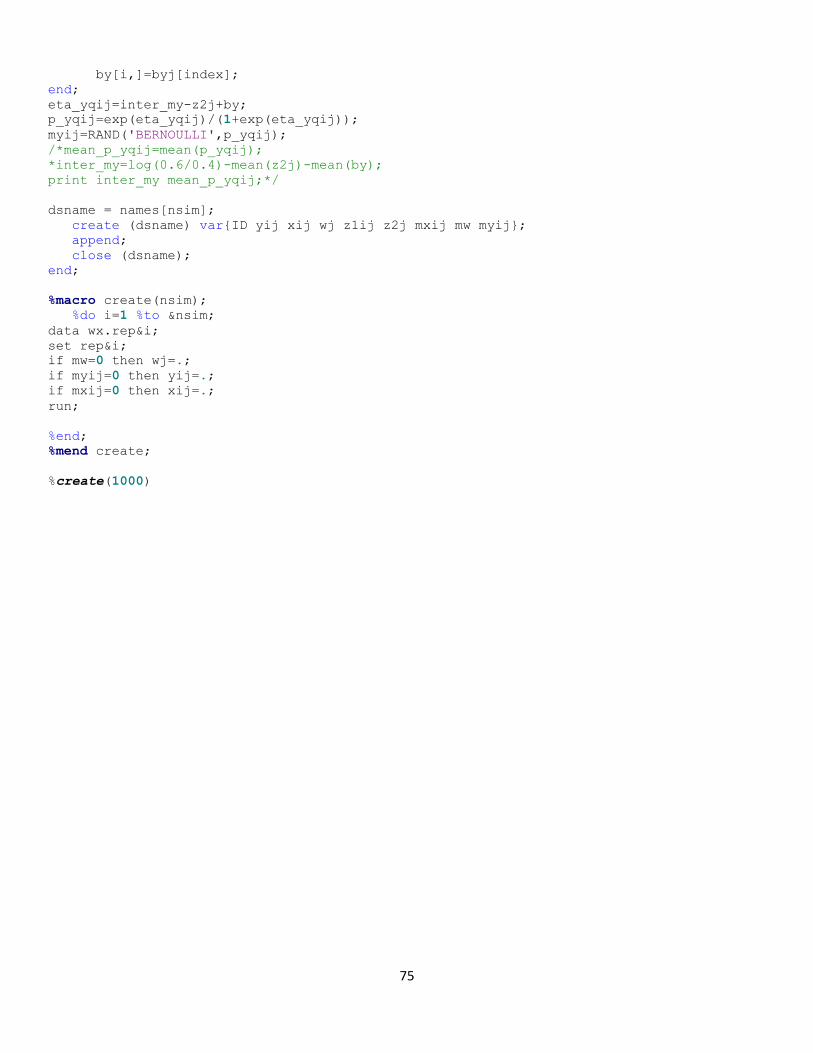
75
by[i,]=byj[index];
end;
eta_yqij=inter_my-z2j+by;
p_yqij=exp(eta_yqij)/(1+exp(eta_yqij));
myij=RAND('BERNOULLI',p_yqij);
/*mean_p_yqij=mean(p_yqij);
*inter_my=log(0.6/0.4)-mean(z2j)-mean(by);
print inter_my mean_p_yqij;*/
dsname = names[nsim];
create (dsname) var{ID yij xij wj z1ij z2j mxij mw myij};
append;
close (dsname);
end;
%macro create(nsim);
%do i=1 %to ≁
data wx.rep&i;
set rep&i;
if mw=0 then wj=.;
if myij=0 then yij=.;
if mxij=0 then xij=.;
run;
%end;
%mend create;
%create(1000)

76
Appendix B
HLM Batch Code in R
The purpose of this code is to show how R package can be used to automate A Monte Carlo simulation using
HLM software.
In this code
.mdmt files (.mdm template file) will be created to convert text files to .mdm files (mdm data file for
HLM).
shell() function in R is used to run HLM in batch mode to convert text files to .mdm files using .mdmt
files.
.hlm files (input command files) will be created to run HLM
shell() function in R is used to run HLM in batch mode to estimate parameters using .hlm files.
From output files, parameter estimates of interest are extracted using the functions in R that support
regular expression.
B. 1 First Simulation Study HLM Batch Code in R
### Specify working director ###
mainfolder<-"C:/HLM
HLM2Path <-"C:/HLM/"
filename<-"Result.csv"
setwd(file.path(mainfolder,"data"))
### Create .mdm file ###
nsim <-1000
for (sim in 1:nsim) {
mdmtFile <- paste("rep",sim,".mdmt",sep="")
write("#HLM2 MDM CREATION TEMPLATE"
,file=file.path(mainfolder,"data",mdmtFile), append=T)
write("mdmtype:0"
,file=file.path(mainfolder,"data",mdmtFile), append=T)
write("rawdattype:other"
,file=file.path(mainfolder,"data",mdmtFile), append=T)
cat("l1fname:C:\\HLM\\data\\rep",sim,".sas7bdat /sas-win\n",sep=""
,file=file.path(mainfolder,"data",mdmtFile), append=T)
cat("l2fname:C:\\HLM\\data\\rep",sim,".sas7bdat /sas-win\n",sep=""
,file=file.path(mainfolder,"data",mdmtFile), append=T)
write("l1missing:y"
,file=file.path(mainfolder,"data",mdmtFile), append=T)
write("timeofdeletion:analysis"
,file=file.path(mainfolder,"data",mdmtFile), append=T)
write(paste("mdmname:","rep",sim,".mdm",sep="")
,file=file.path(mainfolder,"data",mdmtFile), append=T)
write("*begin l1vars"
,file=file.path(mainfolder,"data",mdmtFile), append=T)
write("level2id:ID"
,file=file.path(mainfolder,"data",mdmtFile), append=T)
write("YIJ"
77
,file=file.path(mainfolder,"data",mdmtFile), append=T)
write("XIJ"
,file=file.path(mainfolder,"data",mdmtFile), append=T)
write("*end l1vars"
,file=file.path(mainfolder,"data",mdmtFile), append=T)
write("*begin l2vars"
,file=file.path(mainfolder,"data",mdmtFile), append=T)
write("level2id:ID"
,file=file.path(mainfolder,"data",mdmtFile), append=T)
write("WJ"
,file=file.path(mainfolder,"data",mdmtFile), append=T)
write("*end l2vars"
,file=file.path(mainfolder,"data",mdmtFile), append=T)
}
### Create .hlm input command file ###
nsim <-1000
for (sim in 1:nsim) {
mdmtFile <- paste("rep",sim,".hlm",sep="")
write(paste("#WHLM CMD FILE FOR rep",sim,".mdm",sep="")
,file=file.path(mainfolder,"data",mdmtFile), append=T)
write("nonlin:n"
,file=file.path(mainfolder,"data",mdmtFile), append=T)
write("numit:100"
,file=file.path(mainfolder,"data",mdmtFile), append=T)
write("stopval:0.0000010000"
,file=file.path(mainfolder,"data",mdmtFile), append=T)
write("level1:YIJ=INTRCPT1+XIJ+RANDOM"
,file=file.path(mainfolder,"data",mdmtFile), append=T)
write("level2:INTRCPT1=INTRCPT2+WJ+random/"
,file=file.path(mainfolder,"data",mdmtFile), append=T)
write("level2:XIJ=INTRCPT2/"
,file=file.path(mainfolder,"data",mdmtFile), append=T)
write("fixtau:3"
,file=file.path(mainfolder,"data",mdmtFile), append=T)
write("lev1ols:10"
,file=file.path(mainfolder,"data",mdmtFile), append=T)
write("accel:5"
,file=file.path(mainfolder,"data",mdmtFile), append=T)
write("level1weight:none"
,file=file.path(mainfolder,"data",mdmtFile), append=T)
write("level2weight:none"
,file=file.path(mainfolder,"data",mdmtFile), append=T)
write("varianceknown:none"
,file=file.path(mainfolder,"data",mdmtFile), append=T)
write("level1deletion:none"
,file=file.path(mainfolder,"data",mdmtFile), append=T)
write("hypoth:n"
,file=file.path(mainfolder,"data",mdmtFile), append=T)

78
write("resfil1:n"
,file=file.path(mainfolder,"data",mdmtFile), append=T)
write("resfil2:n"
,file=file.path(mainfolder,"data",mdmtFile), append=T)
write("homvar:n"
,file=file.path(mainfolder,"data",mdmtFile), append=T)
write("constrain:n"
,file=file.path(mainfolder,"data",mdmtFile), append=T)
write("heterol1var:n"
,file=file.path(mainfolder,"data",mdmtFile), append=T)
write("lvr:n"
,file=file.path(mainfolder,"data",mdmtFile), append=T)
write("title:no title"
,file=file.path(mainfolder,"data",mdmtFile), append=T)
write(gsub("/","\\\\",paste("output:",file.path(mainfolder,"data","rep"),sim,".txt",sep=""))
,file=file.path(mainfolder,"data",mdmtFile), append=T)
write("fulloutput:n"
,file=file.path(mainfolder,"data",mdmtFile), append=T)
write("mlf:y"
,file=file.path(mainfolder,"data",mdmtFile), append=T)
write("autoimpute:5"
,file=file.path(mainfolder,"data",mdmtFile), append=T)
write("autoimputeiter:100,y"
,file=file.path(mainfolder,"data",mdmtFile), append=T)
write("autoimputekeep:n,n,n"
,file=file.path(mainfolder,"data",mdmtFile), append=T)
}
### Convert .mdmt file to .mdm template file ###
for (sim in 1:nsim) {
shell(paste(HLM2Path,"hlm2"," -R rep",sim,".mdmt",sep=""))
}
### Run HLM in batch mode ###
for (sim in 1:nsim) {
shell(paste(HLM2Path,"hlm2 ","rep",sim,".mdm ","rep",sim,".hlm",sep=""))
}
### Extract the output and calculate bias and RMSE # outPut1 is a list object in R of which element are the content of each output file (the average file) outPut1 <- lapply(list.files(pattern=".avg"),readLines) # outPut2 contains only portion of output files outPut2 <- lapply(outPut1, function(x) { pointer_loc = grep("with robust standard errors",x); if (length(pointer_loc)>0) return( x[(pointer_loc+6):(pointer_loc+6+14)]) else return(NA) }) # remove unnecessary line 3 from outPut2 outPut3 <- lapply(outPut2, function(x) x[-6])

79
# str_extract_all() will extract only decimal numbers from outPut3 library(stringr) outPut4 <- lapply(outPut3, function(x) str_extract_all(x,"[0-9]+\\.[0-9]+")) # organize outPut4 to be matrix form using do.call() outPut5 <- lapply(outPut4, function(x) do.call("rbind",x)) col1=matrix(0,5,length(outPut5)) for (i in 1:length(outPut5)){ col1[,i]=as.numeric(outPut5[[i]][,1]) } col2=matrix(0,5,length(outPut5)) for (i in 1:length(outPut5)){ col2[,i]=as.numeric(outPut5[[i]][,2]) } col1[which(col1>10)] = NA ### ad-hoc dealing with outlier. col2[which(col2>10)] = NA mean=rowMeans(col1,na.rm=T) mean_random=rowMeans(col2,na.rm=T) bias_b00=mean[1]-1 bias_b01=mean[2]-1 bias_b10=mean[3]-1 bias_u=mean_random[4]-1 bias_r=mean_random[5]-1 rmse_b00=sqrt(mean((col1[1,]-1)**2,na.rm=T)) rmse_b01=sqrt(mean((col1[2,]-1)**2,na.rm=T)) rmse_b10=sqrt(mean((col1[3,]-1)**2,na.rm=T)) rmse_u=sqrt(mean((col2[4,]-1)**2,na.rm=T)) rmse_r=sqrt(mean((col2[5,]-1)**2,na.rm=T)) cbind(bias_b00,bias_b01,bias_b10,bias_u,bias_r,rmse_b00,rmse_b01,rmse_b10,rmse_u,rmse_r)
B.2 Second Simulation Study HLM Batch Code in R
W Model
### Specify working director ###
mainfolder<-"C:/HLM"
HLM2Path <-"C:/HLM/"
setwd(file.path(mainfolder,"data"))
### Create .mdm file ###
nsim <-1000
for (sim in 1:nsim) {
mdmtFile <- paste("rep",sim,".mdmt",sep="")
write("#HLM2 MDM CREATION TEMPLATE"
,file=file.path(mainfolder,"data",mdmtFile), append=T)
write("mdmtype:0"
80
,file=file.path(mainfolder,"data",mdmtFile), append=T)
write("rawdattype:other"
,file=file.path(mainfolder,"data",mdmtFile), append=T)
cat("l1fname:C:\\HLM\\data\\rep",sim,".sas7bdat /sas-win\n",sep="" ##change
,file=file.path(mainfolder,"data",mdmtFile), append=T)
cat("l2fname:C:\\HLM\\data\\rep",sim,".sas7bdat /sas-win\n",sep="" ##change
,file=file.path(mainfolder,"data",mdmtFile), append=T)
write("l1missing:y"
,file=file.path(mainfolder,"data",mdmtFile), append=T)
write("timeofdeletion:analysis"
,file=file.path(mainfolder,"data",mdmtFile), append=T)
write(paste("mdmname:","rep",sim,".mdm",sep="")
,file=file.path(mainfolder,"data",mdmtFile), append=T)
write("*begin l1vars"
,file=file.path(mainfolder,"data",mdmtFile), append=T)
write("level2id:ID"
,file=file.path(mainfolder,"data",mdmtFile), append=T)
write("YIJ"
,file=file.path(mainfolder,"data",mdmtFile), append=T)
write("MYIJ"
,file=file.path(mainfolder,"data",mdmtFile), append=T)
write("*end l1vars"
,file=file.path(mainfolder,"data",mdmtFile), append=T)
write("*begin l2vars"
,file=file.path(mainfolder,"data",mdmtFile), append=T)
write("level2id:ID"
,file=file.path(mainfolder,"data",mdmtFile), append=T)
write("WJ"
,file=file.path(mainfolder,"data",mdmtFile), append=T)
write("Z2J"
,file=file.path(mainfolder,"data",mdmtFile), append=T)
write("*end l2vars"
,file=file.path(mainfolder,"data",mdmtFile), append=T)
}
### Create .hlm input command file ###
for (sim in 1:nsim) {
mdmtFile <- paste("rep",sim,".hlm",sep="")
write(paste("#WHLM CMD FILE FOR rep",sim,".mdm",sep="")
,file=file.path(mainfolder,"data",mdmtFile), append=T)
write("nonlin:n"
,file=file.path(mainfolder,"data",mdmtFile), append=T)
write("numit:100"
,file=file.path(mainfolder,"data",mdmtFile), append=T)
write("stopval:0.0000010000"
,file=file.path(mainfolder,"data",mdmtFile), append=T)
write("level1:YIJ=INTRCPT1+RANDOM"
,file=file.path(mainfolder,"data",mdmtFile), append=T)
write("level2:INTRCPT1=INTRCPT2+WJ+Z2J+random/"

81
,file=file.path(mainfolder,"data",mdmtFile), append=T)
write("fixtau:3"
,file=file.path(mainfolder,"data",mdmtFile), append=T)
write("lev1ols:10"
,file=file.path(mainfolder,"data",mdmtFile), append=T)
write("accel:5"
,file=file.path(mainfolder,"data",mdmtFile), append=T)
write("level1weight:none"
,file=file.path(mainfolder,"data",mdmtFile), append=T)
write("level2weight:none"
,file=file.path(mainfolder,"data",mdmtFile), append=T)
write("varianceknown:none"
,file=file.path(mainfolder,"data",mdmtFile), append=T)
write("level1deletion:none"
,file=file.path(mainfolder,"data",mdmtFile), append=T)
write("hypoth:n"
,file=file.path(mainfolder,"data",mdmtFile), append=T)
write("resfil1:n"
,file=file.path(mainfolder,"data",mdmtFile), append=T)
write("resfil2:n"
,file=file.path(mainfolder,"data",mdmtFile), append=T)
write("homvar:n"
,file=file.path(mainfolder,"data",mdmtFile), append=T)
write("constrain:n"
,file=file.path(mainfolder,"data",mdmtFile), append=T)
write("heterol1var:n"
,file=file.path(mainfolder,"data",mdmtFile), append=T)
write("lvr:n"
,file=file.path(mainfolder,"data",mdmtFile), append=T)
write("title:no title"
,file=file.path(mainfolder,"data",mdmtFile), append=T)
write(gsub("/","\\\\",paste("output:",file.path(mainfolder,"data","rep"),sim,".txt",sep=""))
,file=file.path(mainfolder,"data",mdmtFile), append=T)
write("fulloutput:n"
,file=file.path(mainfolder,"data",mdmtFile), append=T)
write("mlf:y"
,file=file.path(mainfolder,"data",mdmtFile), append=T)
write("autoimpute:5"
,file=file.path(mainfolder,"data",mdmtFile), append=T)
write("autoimputeiter:100,y"
,file=file.path(mainfolder,"data",mdmtFile), append=T)
write("autoimputekeep:n,n,n"
,file=file.path(mainfolder,"data",mdmtFile), append=T)
}
### Convert .mdmt file to .mdm template file ###
for (sim in 1:nsim) {
shell(paste(HLM2Path,"hlm2"," -R rep",sim,".mdmt",sep=""))
}
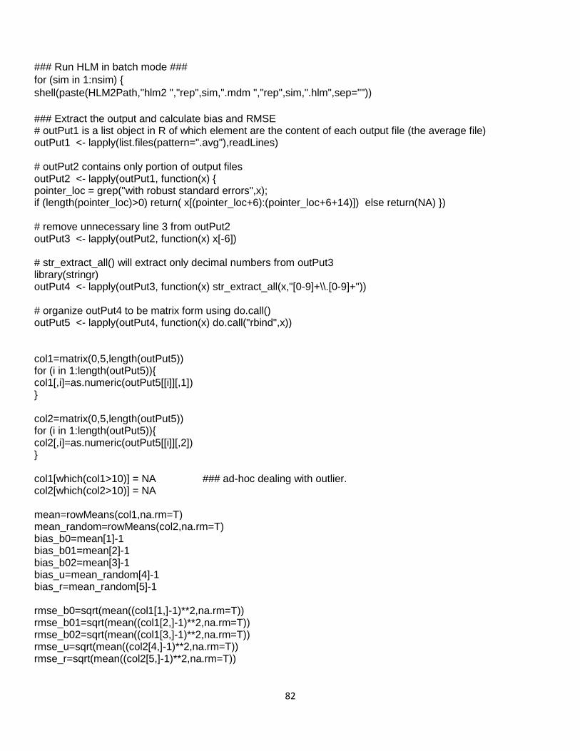
82
### Run HLM in batch mode ###
for (sim in 1:nsim) {
shell(paste(HLM2Path,"hlm2 ","rep",sim,".mdm ","rep",sim,".hlm",sep=""))
### Extract the output and calculate bias and RMSE # outPut1 is a list object in R of which element are the content of each output file (the average file) outPut1 <- lapply(list.files(pattern=".avg"),readLines) # outPut2 contains only portion of output files outPut2 <- lapply(outPut1, function(x) { pointer_loc = grep("with robust standard errors",x); if (length(pointer_loc)>0) return( x[(pointer_loc+6):(pointer_loc+6+14)]) else return(NA) }) # remove unnecessary line 3 from outPut2 outPut3 <- lapply(outPut2, function(x) x[-6]) # str_extract_all() will extract only decimal numbers from outPut3 library(stringr) outPut4 <- lapply(outPut3, function(x) str_extract_all(x,"[0-9]+\\.[0-9]+")) # organize outPut4 to be matrix form using do.call() outPut5 <- lapply(outPut4, function(x) do.call("rbind",x)) col1=matrix(0,5,length(outPut5)) for (i in 1:length(outPut5)){ col1[,i]=as.numeric(outPut5[[i]][,1]) } col2=matrix(0,5,length(outPut5)) for (i in 1:length(outPut5)){ col2[,i]=as.numeric(outPut5[[i]][,2]) } col1[which(col1>10)] = NA ### ad-hoc dealing with outlier. col2[which(col2>10)] = NA mean=rowMeans(col1,na.rm=T) mean_random=rowMeans(col2,na.rm=T) bias_b0=mean[1]-1 bias_b01=mean[2]-1 bias_b02=mean[3]-1 bias_u=mean_random[4]-1 bias_r=mean_random[5]-1 rmse_b0=sqrt(mean((col1[1,]-1)**2,na.rm=T)) rmse_b01=sqrt(mean((col1[2,]-1)**2,na.rm=T)) rmse_b02=sqrt(mean((col1[3,]-1)**2,na.rm=T)) rmse_u=sqrt(mean((col2[4,]-1)**2,na.rm=T)) rmse_r=sqrt(mean((col2[5,]-1)**2,na.rm=T))
83
cbind(bias_b0,bias_b01,bias_b02,bias_u,bias_r,rmse_b0,rmse_b01,rmse_b02,rmse_u,rmse_r) X Model
### Specify working director ###
mainfolder<-"C:/HLM"
HLM2Path <-"C:/HLM/"
setwd(file.path(mainfolder,"data"))
### Create .mdm file ###
nsim <-1000
for (sim in 1:nsim) {
mdmtFile <- paste("rep",sim,".mdmt",sep="")
write("#HLM2 MDM CREATION TEMPLATE"
,file=file.path(mainfolder,"data",mdmtFile), append=T)
write("mdmtype:0"
,file=file.path(mainfolder,"data",mdmtFile), append=T)
write("rawdattype:other"
,file=file.path(mainfolder,"data",mdmtFile), append=T)
cat("l1fname:C:\\HLM\\data\\rep",sim,".sas7bdat /sas-win\n",sep=""
,file=file.path(mainfolder,"data",mdmtFile), append=T)
cat("l2fname:C:\\HLM\\data\\rep",sim,".sas7bdat /sas-win\n",sep=""
,file=file.path(mainfolder,"data",mdmtFile), append=T)
write("l1missing:y"
,file=file.path(mainfolder,"data",mdmtFile), append=T)
write("timeofdeletion:analysis"
,file=file.path(mainfolder,"data",mdmtFile), append=T)
write(paste("mdmname:","rep",sim,".mdm",sep="")
,file=file.path(mainfolder,"data",mdmtFile), append=T)
write("*begin l1vars"
,file=file.path(mainfolder,"data",mdmtFile), append=T)
write("level2id:ID"
,file=file.path(mainfolder,"data",mdmtFile), append=T)
write("YIJ"
,file=file.path(mainfolder,"data",mdmtFile), append=T)
write("XIJ"
,file=file.path(mainfolder,"data",mdmtFile), append=T)
write("Z1IJ"
,file=file.path(mainfolder,"data",mdmtFile), append=T)
write("*end l1vars"
,file=file.path(mainfolder,"data",mdmtFile), append=T)
write("*begin l2vars"
,file=file.path(mainfolder,"data",mdmtFile), append=T)
write("level2id:ID"
,file=file.path(mainfolder,"data",mdmtFile), append=T)
write("Z2J"
,file=file.path(mainfolder,"data",mdmtFile), append=T)
write("*end l2vars"
,file=file.path(mainfolder,"data",mdmtFile), append=T)
}

84
### Create .hlm input command file ###
for (sim in 1:nsim) {
mdmtFile <- paste("rep",sim,".hlm",sep="")
write(paste("#WHLM CMD FILE FOR rep",sim,".mdm",sep="")
,file=file.path(mainfolder,"data",mdmtFile), append=T)
write("nonlin:n"
,file=file.path(mainfolder,"data",mdmtFile), append=T)
write("numit:100"
,file=file.path(mainfolder,"data",mdmtFile), append=T)
write("stopval:0.0000010000"
,file=file.path(mainfolder,"data",mdmtFile), append=T)
write("level1:YIJ=INTRCPT1+XIJ+Z1IJ+RANDOM"
,file=file.path(mainfolder,"data",mdmtFile), append=T)
write("level2:INTRCPT1=INTRCPT2+random/"
,file=file.path(mainfolder,"data",mdmtFile), append=T)
write("level2:XIJ=INTRCPT2/"
,file=file.path(mainfolder,"data",mdmtFile), append=T)
write("level2:Z1IJ=INTRCPT2/"
,file=file.path(mainfolder,"data",mdmtFile), append=T)
write("fixtau:3"
,file=file.path(mainfolder,"data",mdmtFile), append=T)
write("lev1ols:10"
,file=file.path(mainfolder,"data",mdmtFile), append=T)
write("accel:5"
,file=file.path(mainfolder,"data",mdmtFile), append=T)
write("level1weight:none"
,file=file.path(mainfolder,"data",mdmtFile), append=T)
write("level2weight:none"
,file=file.path(mainfolder,"data",mdmtFile), append=T)
write("varianceknown:none"
,file=file.path(mainfolder,"data",mdmtFile), append=T)
write("level1deletion:none"
,file=file.path(mainfolder,"data",mdmtFile), append=T)
write("hypoth:n"
,file=file.path(mainfolder,"data",mdmtFile), append=T)
write("resfil1:n"
,file=file.path(mainfolder,"data",mdmtFile), append=T)
write("resfil2:n"
,file=file.path(mainfolder,"data",mdmtFile), append=T)
write("homvar:n"
,file=file.path(mainfolder,"data",mdmtFile), append=T)
write("constrain:n"
,file=file.path(mainfolder,"data",mdmtFile), append=T)
write("heterol1var:n"
,file=file.path(mainfolder,"data",mdmtFile), append=T)
write("lvr:n"
,file=file.path(mainfolder,"data",mdmtFile), append=T)
write("title:no title"

85
,file=file.path(mainfolder,"data",mdmtFile), append=T)
write(gsub("/","\\\\",paste("output:",file.path(mainfolder,"data","rep"),sim,".txt",sep=""))
,file=file.path(mainfolder,"data",mdmtFile), append=T)
write("fulloutput:n"
,file=file.path(mainfolder,"data",mdmtFile), append=T)
write("mlf:y"
,file=file.path(mainfolder,"data",mdmtFile), append=T)
write("autoimpute:5"
,file=file.path(mainfolder,"data",mdmtFile), append=T)
write("autoimputeiter:100,y"
,file=file.path(mainfolder,"data",mdmtFile), append=T)
write("autoimputekeep:n,n,n"
,file=file.path(mainfolder,"data",mdmtFile), append=T)
}
### Convert .mdmt file to .mdm template file ###
for (sim in 1:nsim) {
shell(paste(HLM2Path,"hlm2"," -R rep",sim,".mdmt",sep=""))
}
### Run HLM in batch mode ###
for (sim in 1:nsim) {
shell(paste(HLM2Path,"hlm2 ","rep",sim,".mdm ","rep",sim,".hlm",sep=""))
}
### Extract the output and calculate bias and RMSE # outPut1 is a list object in R of which element are the content of each output file (the average file) outPut1 <- lapply(list.files(pattern=".avg"),readLines) # outPut2 contains only portion of output files outPut2 <- lapply(outPut1, function(x) { pointer_loc = grep("with robust standard errors",x); if (length(pointer_loc)>0) return( x[(pointer_loc+6):(pointer_loc+6+15)]) else return(NA) }) # remove unnecessary line 3 from outPut2 outPut3 <- lapply(outPut2, function(x) x[-6]) # str_extract_all() will extract only decimal numbers from outPut3 library(stringr) outPut4 <- lapply(outPut3, function(x) str_extract_all(x,"[0-9]+\\.[0-9]+")) # organize outPut4 to be matrix form using do.call() outPut5 <- lapply(outPut4, function(x) do.call("rbind",x)) col1=matrix(0,5,length(outPut5)) for (i in 1:length(outPut5)){ col1[,i]=as.numeric(outPut5[[i]][,1]) } col2=matrix(0,5,length(outPut5)) for (i in 1:length(outPut5)){

86
col2[,i]=as.numeric(outPut5[[i]][,2]) } col1[which(col1>10)] = NA ### ad-hoc dealing with outlier. col2[which(col2>10)] = NA mean=rowMeans(col1,na.rm=T) mean_random=rowMeans(col2,na.rm=T) bias_b00=mean[1]-1 bias_b10=mean[2]-1 bias_b20=mean[3]-1 bias_u=mean_random[4]-1 bias_r=mean_random[5]-1 rmse_b00=sqrt(mean((col1[1,]-1)**2,na.rm=T)) rmse_b01=sqrt(mean((col1[2,]-1)**2,na.rm=T)) rmse_b10=sqrt(mean((col1[3,]-1)**2,na.rm=T)) rmse_u=sqrt(mean((col2[4,]-1)**2,na.rm=T)) rmse_r=sqrt(mean((col2[5,]-1)**2,na.rm=T)) cbind(bias_b00,bias_b10,bias_b20,bias_u,bias_r,rmse_b00,rmse_b01,rmse_b10,rmse_u,rmse_r)
W and X Model
### Specify working director ###
mainfolder<-"C:/HLM/"
HLM2Path <-"C:/HLM/"
setwd(file.path(mainfolder,"data"))
### Create .mdm file ###
nsim <-1000
for (sim in 1:nsim) {
mdmtFile <- paste("rep",sim,".mdmt",sep="")
write("#HLM2 MDM CREATION TEMPLATE"
,file=file.path(mainfolder,"data",mdmtFile), append=T)
write("mdmtype:0"
,file=file.path(mainfolder,"data",mdmtFile), append=T)
write("rawdattype:other"
,file=file.path(mainfolder,"data",mdmtFile), append=T)
cat("l1fname:C:\\HLM\\data\\rep",sim,".sas7bdat /sas-win\n",sep=""
,file=file.path(mainfolder,"data",mdmtFile), append=T)
cat("l2fname:C:\\HLM\\data\\rep",sim,".sas7bdat /sas-win\n",sep=""
,file=file.path(mainfolder,"data",mdmtFile), append=T)
write("l1missing:y"
,file=file.path(mainfolder,"data",mdmtFile), append=T)
write("timeofdeletion:analysis"
,file=file.path(mainfolder,"data",mdmtFile), append=T)
write(paste("mdmname:","rep",sim,".mdm",sep="")
,file=file.path(mainfolder,"data",mdmtFile), append=T)
write("*begin l1vars"
,file=file.path(mainfolder,"data",mdmtFile), append=T)

87
write("level2id:ID"
,file=file.path(mainfolder,"data",mdmtFile), append=T)
write("YIJ"
,file=file.path(mainfolder,"data",mdmtFile), append=T)
write("XIJ"
,file=file.path(mainfolder,"data",mdmtFile), append=T)
write("Z1IJ"
,file=file.path(mainfolder,"data",mdmtFile), append=T)
write("*end l1vars"
,file=file.path(mainfolder,"data",mdmtFile), append=T)
write("*begin l2vars"
,file=file.path(mainfolder,"data",mdmtFile), append=T)
write("level2id:ID"
,file=file.path(mainfolder,"data",mdmtFile), append=T)
write("WJ"
,file=file.path(mainfolder,"data",mdmtFile), append=T)
write("Z2J"
,file=file.path(mainfolder,"data",mdmtFile), append=T)
write("*end l2vars"
,file=file.path(mainfolder,"data",mdmtFile), append=T)
}
### Create .hlm input command file ###
for (sim in 1:nsim) {
mdmtFile <- paste("rep",sim,".hlm",sep="")
write(paste("#WHLM CMD FILE FOR rep",sim,".mdm",sep="")
,file=file.path(mainfolder,"data",mdmtFile), append=T)
write("nonlin:n"
,file=file.path(mainfolder,"data",mdmtFile), append=T)
write("numit:100"
,file=file.path(mainfolder,"data",mdmtFile), append=T)
write("stopval:0.0000010000"
,file=file.path(mainfolder,"data",mdmtFile), append=T)
write("level1:YIJ=INTRCPT1+XIJ+Z1IJ+RANDOM"
,file=file.path(mainfolder,"data",mdmtFile), append=T)
write("level2:INTRCPT1=INTRCPT2+WJ+Z2J+random/"
,file=file.path(mainfolder,"data",mdmtFile), append=T)
write("level2:XIJ=INTRCPT2/"
,file=file.path(mainfolder,"data",mdmtFile), append=T)
write("level2:Z1IJ=INTRCPT2/"
,file=file.path(mainfolder,"data",mdmtFile), append=T)
write("fixtau:3"
,file=file.path(mainfolder,"data",mdmtFile), append=T)
write("lev1ols:10"
,file=file.path(mainfolder,"data",mdmtFile), append=T)
write("accel:5"
,file=file.path(mainfolder,"data",mdmtFile), append=T)
write("level1weight:none"
,file=file.path(mainfolder,"data",mdmtFile), append=T)
88
write("level2weight:none"
,file=file.path(mainfolder,"data",mdmtFile), append=T)
write("varianceknown:none"
,file=file.path(mainfolder,"data",mdmtFile), append=T)
write("level1deletion:none"
,file=file.path(mainfolder,"data",mdmtFile), append=T)
write("hypoth:n"
,file=file.path(mainfolder,"data",mdmtFile), append=T)
write("resfil1:n"
,file=file.path(mainfolder,"data",mdmtFile), append=T)
write("resfil2:n"
,file=file.path(mainfolder,"data",mdmtFile), append=T)
write("homvar:n"
,file=file.path(mainfolder,"data",mdmtFile), append=T)
write("constrain:n"
,file=file.path(mainfolder,"data",mdmtFile), append=T)
write("heterol1var:n"
,file=file.path(mainfolder,"data",mdmtFile), append=T)
write("lvr:n"
,file=file.path(mainfolder,"data",mdmtFile), append=T)
write("title:no title"
,file=file.path(mainfolder,"data",mdmtFile), append=T)
write(gsub("/","\\\\",paste("output:",file.path(mainfolder,"data","rep"),sim,".txt",sep=""))
,file=file.path(mainfolder,"data",mdmtFile), append=T)
write("fulloutput:n"
,file=file.path(mainfolder,"data",mdmtFile), append=T)
write("mlf:y"
,file=file.path(mainfolder,"data",mdmtFile), append=T)
write("autoimpute:5"
,file=file.path(mainfolder,"data",mdmtFile), append=T)
write("autoimputeiter:100,y"
,file=file.path(mainfolder,"data",mdmtFile), append=T)
write("autoimputekeep:n,n,n"
,file=file.path(mainfolder,"data",mdmtFile), append=T)
}
### Convert .mdmt file to .mdm template file ###
for (sim in 1:nsim) {
shell(paste(HLM2Path,"hlm2"," -R rep",sim,".mdmt",sep=""))
}
### Run HLM in batch mode ###
for (sim in 1:nsim) {
shell(paste(HLM2Path,"hlm2 ","rep",sim,".mdm ","rep",sim,".hlm",sep=""))
}
### Extract the output and calculate bias and RMSE # outPut1 is a list object in R of which element are the content of each output file (the average file) outPut1 <- lapply(list.files(pattern=".avg"),readLines)

89
# outPut2 contains only portion of output files outPut2 <- lapply(outPut1, function(x) { pointer_loc = grep("with robust standard errors",x); if (length(pointer_loc)>0) return( x[(pointer_loc+6):(pointer_loc+6+18)]) else return(NA) }) # remove unnecessary line 3 from outPut2 outPut3 <- lapply(outPut2, function(x) x[-6]) # str_extract_all() will extract only decimal numbers from outPut3 library(stringr) outPut4 <- lapply(outPut3, function(x) str_extract_all(x,"[0-9]+\\.[0-9]+")) # organize outPut4 to be matrix form using do.call() outPut5 <- lapply(outPut4, function(x) do.call("rbind",x)) col1=matrix(0,7,length(outPut5)) for (i in 1:length(outPut5)){ col1[,i]=as.numeric(outPut5[[i]][,1]) } col2=matrix(0,7,length(outPut5)) for (i in 1:length(outPut5)){ col2[,i]=as.numeric(outPut5[[i]][,2]) } col1[which(col1>10)] = NA ### ad-hoc dealing with outlier. col2[which(col2>10)] = NA mean=rowMeans(col1,na.rm=T) mean_random=rowMeans(col2,na.rm=T) bias_b0=mean[1]-1 bias_b01=mean[2]-1 bias_b02=mean[3]-1 bias_b10=mean[4]-1 bias_b20=mean[5]-1 bias_u=mean_random[6]-1 bias_r=mean_random[7]-1 rmse_b0=sqrt(mean((col1[1,]-1)**2,na.rm=T)) rmse_b01=sqrt(mean((col1[2,]-1)**2,na.rm=T)) rmse_b02=sqrt(mean((col1[3,]-1)**2,na.rm=T)) rmse_b10=sqrt(mean((col1[4,]-1)**2,na.rm=T)) rmse_b20=sqrt(mean((col1[5,]-1)**2,na.rm=T)) rmse_u=sqrt(mean((col2[6,]-1)**2,na.rm=T)) rmse_r=sqrt(mean((col2[7,]-1)**2,na.rm=T)) cbind(bias_b0,bias_b01,bias_b02,bias_b10,bias_b20,bias_u,bias_r,rmse_b0,rmse_b01,rmse_b02,rmse_b10,rmse_b20,rmse_u,rmse_r)