This article was downloaded by: [Stony Brook University]On: 22 October 2014, At: 04:05Publisher: Taylor & FrancisInforma Ltd Registered in England and Wales Registered Number: 1072954 Registered office: MortimerHouse, 37-41 Mortimer Street, London W1T 3JH, UK

Journal of the American Statistical AssociationPublication details, including instructions for authors and subscription information:http://www.tandfonline.com/loi/uasa20

Sensitivity Analysis for Instrumental VariablesRegression With Overidentifying RestrictionsDylan S Smallaa Dylan S. Small is Assistant Professor, Department of Statistics, The Wharton School ofthe University of Pennsylvania, Philadelphia, PA 19104 . The author is grateful to RobertStine and Tom Ten Have for valuable comments on a draft and to Joshua Angrist, EdGeorge, and Paul Rosenbaum for insightful discussions. He also thanks the associateeditor and three referees for helpful comments.Published online: 01 Jan 2012.

To cite this article: Dylan S Small (2007) Sensitivity Analysis for Instrumental Variables Regression With OveridentifyingRestrictions, Journal of the American Statistical Association, 102:479, 1049-1058, DOI: 10.1198/016214507000000608

To link to this article: http://dx.doi.org/10.1198/016214507000000608

PLEASE SCROLL DOWN FOR ARTICLE

Taylor & Francis makes every effort to ensure the accuracy of all the information (the “Content”) containedin the publications on our platform. However, Taylor & Francis, our agents, and our licensors make norepresentations or warranties whatsoever as to the accuracy, completeness, or suitability for any purpose ofthe Content. Any opinions and views expressed in this publication are the opinions and views of the authors,and are not the views of or endorsed by Taylor & Francis. The accuracy of the Content should not be reliedupon and should be independently verified with primary sources of information. Taylor and Francis shallnot be liable for any losses, actions, claims, proceedings, demands, costs, expenses, damages, and otherliabilities whatsoever or howsoever caused arising directly or indirectly in connection with, in relation to orarising out of the use of the Content.

This article may be used for research, teaching, and private study purposes. Any substantial or systematicreproduction, redistribution, reselling, loan, sub-licensing, systematic supply, or distribution in anyform to anyone is expressly forbidden. Terms & Conditions of access and use can be found at http://www.tandfonline.com/page/terms-and-conditions

Sensitivity Analysis for Instrumental VariablesRegression With Overidentifying Restrictions

Dylan S. SMALL

Instrumental variables regression (IV regression) is a method for making causal inferences about the effect of a treatment based on anobservational study in which there are unmeasured confounding variables. The method requires one or more valid instrumental variables(IVs); a valid IV is a variable that is associated with the treatment, is independent of unmeasured confounding variables, and has no directeffect on the outcome. Often there is uncertainty about the validity of the proposed IVs. When a researcher proposes more than one IV, thevalidity of these IVs can be tested through the “overidentifying restrictions test.” Although the overidentifying restrictions test does providesome information, the test has no power versus certain alternatives and can have low power versus many alternatives due to its omnibusnature. To fully address uncertainty about the validity of the proposed IVs, we argue that a sensitivity analysis is needed. A sensitivityanalysis examines the impact of plausible amounts of invalidity of the proposed IVs on inferences for the parameters of interest. We developa method of sensitivity analysis for IV regression with overidentifying restrictions that makes full use of the information provided by theoveridentifying restrictions test but provides more information than the test by exploring sensitivity to violations of the validity of theproposed IVs in directions for which the test has low power. Our sensitivity analysis uses interpretable parameters that can be discussedwith subject matter experts. We illustrate our method using a study of food demand among rural households in the Philippines.

KEY WORDS: Causal inference; Econometrics; Structural equations models.

1. INTRODUCTION

A fundamental problem in making inferences about thecausal effect of a treatment based on observational data is thepotential presence of unmeasured confounding variables. In-strumental variables regression (IV regression) is a method forovercoming this problem. The method requires a valid instru-mental variable (IV), which is a variable that is associated withthe treatment, is independent of the unmeasured confoundingvariables, and has no direct effect on the outcome. IV regres-sion uses the IV to extract variation in the treatment that is un-related to the unmeasured confounding variables and then usesthis variation to estimate the causal effect of the treatment. Anexample is the study of Card (1995) on the causal effect of edu-cation earnings that uses the distance a person lived when grow-ing up from the nearest 4-year college as an IV.

In many applications of IV regression, researchers are uncer-tain about the validity of the proposed IV. For example, Card(1995) was concerned that families that place a strong empha-sis on education are more likely to choose to live near a col-lege, and that children in these families are more likely to bemotivated to achieve labor market success. Under this scenario,the proposed IV (distance from nearest 4-year college) wouldbe associated with an unmeasured confounding variable (moti-vation), meaning that the proposed IV would be invalid. Thevalidity of a proposed IV cannot be tested consistently (seeSec. 3.1). When critical assumptions for an analysis are par-tially unverifiable, a sensitivity analysis is useful. A sensitivityanalysis examines the impact of plausible (in the view of subjectmatter experts) violations of the assumptions. The value of do-ing a sensitivity analysis to address uncertainty about partiallyunverifiable assumptions has long been recognized in causal in-ference (see Rosenbaum 2002, chap. 4, for a review). Sensi-tivity analyses for IV regression have been considered by Man-ski (1995), Angrist, Imbens, and Rubin (1996), and Rosenbaum(1999).

Dylan S. Small is Assistant Professor, Department of Statistics, The Whar-ton School of the University of Pennsylvania, Philadelphia, PA 19104 (E-mail:dsmall@wharton.upenn.edu). The author is grateful to Robert Stine and TomTen Have for valuable comments on a draft and to Joshua Angrist, Ed George,and Paul Rosenbaum for insightful discussions. He also thanks the associateeditor and three referees for helpful comments.

In this article we develop a method of sensitivity analysisfor IV regression when there is more than one proposed IV, asetting not considered by previous studies of IV regression sen-sitivity analysis. IV regression with more than one proposed IVis called IV regression with overidentifying restrictions, becauseonly one valid IV is needed to identify the causal effect of treat-ment, so more than one IV “overidentifies” the causal effect.IV regression with overidentifying restrictions is often used ineconomics. An example is the work of Kane and Rouse (1993),who studied the causal effect of education on earnings as Card(1995) did, but, in addition to distance from nearest 4-year col-lege, used tuition at state colleges of the state in which a persongrew up as an IV. For IV regression with overidentifying restric-tions, all of the proposed IVs must be valid for the inferences tobe correct. Although this is a more stringent requirement thanone proposed IV being valid, there are two benefits to consid-ering multiple proposed IVs (Davidson and MacKinnon 1993).First, if all of the proposed IVs are valid, then the use of multi-ple IVs can increase efficiency (see Sec. 2). Second, the use ofmultiple proposed IVs enables testing of the joint validity of allof the proposed IVs (to a limited extent) through the overiden-tifying restrictions test (ORT) (see Sec. 3).

For IV regression with overidentifying restrictions, it is com-mon practice to report inferences that assume that all of theproposed IVs are valid along with the p value for the ORT.However, the results of the ORT are hard to interpret, becausethe test may have low power for many alternatives and is noteven consistent for some alternatives. Consequently, a sensitiv-ity analysis remains essential for addressing uncertainty aboutthe validity of the proposed IVs when multiple proposed IVsare considered. We develop in this article a method of sensitiv-ity analysis that uses the information provided by the ORT, butprovides more information than the test by also exploring thesensitivity of inferences to violations of assumptions in direc-tions for which the test has low power.

The article is organized as follows. In Section 2 we describea model for IV regression and inferences for it. In Section 3

© 2007 American Statistical AssociationJournal of the American Statistical Association

September 2007, Vol. 102, No. 479, Theory and MethodsDOI 10.1198/016214507000000608

1049

Dow

nloa

ded

by [

Ston

y B

rook

Uni

vers

ity]

at 0

4:05

22

Oct

ober

201

4

1050 Journal of the American Statistical Association, September 2007

we describe the ORT and its power, and in Section 4 we de-velop our method of sensitivity analysis. In Section 5 we dis-cuss extensions of our method to IV regression with heteroge-neous treatment effects and/or panel data, and in Section 6 weillustrate our sensitivity analysis method using a study of fooddemand. We provide conclusions and discussion in Section 7.

2. INSTRUMENTAL VARIABLESREGRESSION MODEL

In this section we describe an additive, linear, constant-effectcausal model and explain how valid IVs enable identificationof the model. For defining causal effects, we use the potentialoutcomes approach (Neyman 1923; Rubin 1974). Let y denotean outcome and w denote a treatment variable that an inter-vention could in principle alter. For example, in the study ofKane and Rouse (1993) y is earnings, w is amount of educa-tion, and the intervention that could alter w is for an individualto choose to acquire more or less education. Let y

(w∗)i denote

the outcome that would be observed for unit i if unit i’s levelof w was set equal to w∗. We assume that the potential out-comes for unit i depend only on the level of w set for unit i

and not on the levels of w set for other units—this is called thestable unit treatment value assumption by Rubin (1986). Letyobsi := yi and wobs

i := wi denote the observed values of y andw for unit i. Each unit has a vector of potential outcomes, onefor each possible level of w, but we observe only one potentialoutcome, yi = y

(wi)i . An additive, linear constant-effect causal

model for the potential outcomes (as in Holland 1988) is

y(w∗)i = y

(0)i + βw∗. (1)

Our parameter of interest is β = y(w∗+1)i − y

(w∗)i , the causal

effect of increasing w by one unit. One way to estimate β

is ordinary least squares (OLS) regression of yobs on wobs.The OLS coefficient on w, βOLS, has probability limit β +cov(wobs

i , y(0)i )/var(wobs

i ). If wobsi were randomly assigned,

then cov(wobsi , y

(0)i ) would equal 0, and βOLS would be con-

sistent. But in an observational study, often cov(wobsi , y

(0)i ) �= 0

and βOLS is inconsistent. One strategy to address this problemis to attempt to collect data on all confounding variables q andthen regress yobs on wobs and q. If wobs is conditionally inde-pendent of y(0) given q [i.e., the mechanism of assigning treat-ments wobs is ignorable (Rubin 1978)] and the regression func-tion is specified correctly, then this strategy produces a consis-tent estimate of β . However, it often difficult to figure out and/orcollect all confounding variables q.

IV regression is another strategy for estimating β in (1).A vector of valid IVs zi is a vector of variables that satisfiesthe following assumptions (see Angrist et al. 1996; Tan 2006):

(A1) zi is associated with the observed treatment wobsi .

(A2) zi is independent of {y(w∗)i ,w∗ ∈ W} where W is the

set of possible values of w. Note that under model (1),this is equivalent to zi being independent of y

(0)i .

The basic idea of IV regression is to use z to extract variationin wobs that is independent of the confounding variables and touse only this part of the variation in wobs to estimate the causalrelationship between w and y. Assumption (A1) is needed to

be able to use z to extract variation in wobs and (A2) is neededfor the variation in wobs extracted from variation in z to be in-dependent of the confounding variables.

An example of the usefulness of IVs is the encouragementdesign (Holland 1988). An encouragement design is used whenwe want to estimate the causal effect of a treatment w that wecannot control, but we can control (or observe from a naturalexperiment) variable(s) z which, depending on their level, en-courage or do not encourage a unit to have a high level of wobs.If the levels of the encouragement variables z are randomly as-signed (or the mechanism of assigning the encouragement vari-ables is ignorable) and encouragement in and of itself has nodirect effect on the outcome, then z is a vector of valid IVs (Hol-land 1988; Angrist et al. 1996). The model of Kane and Rouse(1993) can be viewed as an encouragement design in which it isassumed that the mechanism of assigning distance from nearest4-year college and tuition at state colleges where a person grewup is ignorable, and that low levels of these variables encouragea person to attend college but have no direct effect on earnings.

For assumption (A2) to be plausible, it is often necessary tocondition on a vector of covariates xi (Tan 2006). For example,Kane and Rouse (1993) conditioned on region, city size, andfamily background, because these variables may be associatedwith both potential earnings outcomes y

(w∗)i and distance from

nearest 4-year college (and/or tuition at state colleges). Condi-tioning on xi also can increase the efficiency of the IV regres-sion estimator. We call the variables in xi the included exoge-nous variables. We consider a linear model for E(y

(0)i |xi , zi ),

y(w∗)i = βw∗ + δT xi + λT zi + ui, E(ui |xi , zi ) = 0. (2)

We assume that (wi,xi , zi , ui) are iid random vectors. Thismodel has been considered by Holland (1988), among others.The model for the observed data is

yi = βwi + δT xi + λT zi + ui, E(ui |xi , zi ) = 0,

(wi,xi , zi , ui), i = 1, . . . ,N, are iid random vectors. (3)

For this model, we say that z is a vector of valid IVs if it satisfiesassumptions (A1′) and (A2′), which are analogous to (A1) and(A2):

(A1′) The partial R2 for z in the population regression ofwobs on x and z is greater than 0.

(A2′) The vector λ in (3) equals 0.

(A1′) says that z is associated with wobs conditional onx. (A2′) says that z is uncorrelated with the composite u ofthe confounding variables besides x. A sufficient condition for(A2′) to hold is that z is uncorrelated with any of the confound-ing variables besides those in x and that z itself has no directeffect on the outcome (Angrist et al. 1996).

We now consider inferences for β under the assumption thatz is a vector of valid IVs. Under regularity conditions, β can beconsistently estimated by the two-stage least squares (TSLS)method (White 1982; Hausman 1983). The TSLS estimatoris based on the fact that if λ = 0 in (3), then E∗(y|x, z) =βE∗(w|x, z) + δT x, where E∗ denotes linear projection. TheTSLS estimator is obtained by regressing w on (x, z) using OLSto obtain E∗(w|x, z), then regressing y on E∗(w|x, z) and x

Dow

nloa

ded

by [

Ston

y B

rook

Uni

vers

ity]

at 0

4:05

22

Oct

ober

201

4

Small: Instrumental Variables Regression With Overidentifying Restrictions 1051

using OLS to estimate β and δ. The asymptotic distribution ofβTSLS is

√N(βTSLS − β)

σ 2u

∑Ni=1(wi − E∗(w|xi ))2

D→ N(0,1), (4)

where wi is the predicted wi from the OLS regression of wobs

on x and z, E∗(w|x) is the estimated linear projection of w

onto x, and σ 2u = (1/N)

∑Ni=1(yi − βTSLSwi − δ

T

TSLSxi )2. An

asymptotically valid confidence interval (CI) can be obtainedby inverting the Wald test based on (4). Note that the validityof these inferences for β does not require that E(y

(0)i |xi , zi ) be

a linear function of (x, z). Let E∗(y(0)i |xi , zi ) = δT xi + λT zi .

In addition, let u′i = y

(0)i − E∗(y(0)

i |xi , zi ) and assume that theu′

i ’s are iid. Then under conditions (A1′) and (A2′), the TSLSestimator is consistent, and the Wald CI is asymptotically valid(Davidson and MacKinnon 1993).

Using additional valid IVs can increase the efficiency of theTSLS estimator. For fixed x1, . . . ,xN , the denominator of theleft side of (4) is proportional to the partial R2 for z from theOLS regression of wobs on x and z. Thus, using additionalvalid IVs that increase this partial R2 increases the efficiencyof βTSLS.

In the rest of this article, we assume that assumption (A1′)holds for the vector of proposed IVs z but consider the im-pact on inferences of (A2′) being violated for z. (A2′) be-ing violated means that λ �= 0, which means that z is asso-ciated with a confounding variable(s) not in x and/or z hasa direct effect on the outcome. If λ �= 0, then (βTSLS, δTSLS)

is not typically a consistent estimator of (β, δ). Let YN =(y1, . . . , yN)T , WN = (w1, . . . ,wN)T , XN = (x1, . . . ,xN)T ,ZN = (z1, . . . , zN)T , and DN = [XN,ZN ]. The asymptotic bias

of βTSLS, δT

TSLS is

limN→∞

{([DN(DTN DN)−1DT

N WN,XN ]T

× [DN(DTN DN)−1DT

NWN,XN ])−1

× [DN(DTN DN)−1DT

NWN,XN ]T ZNλ}. (5)

Before further considering the affect of λ not being equal to 0on inferences, we consider a test of whether λ equals 0.

3. OVERIDENTIFYING RESTRICTIONS TESTAND ITS POWER

An ORT is a test of the assumption that λ = 0 in (3), whichcan be applied when dim(z) > 1. ORTs derives their name fromthe fact that when dim(z) > 1 and λ = 0, the parameter β in(3) is “overidentified,” meaning that any nonempty subset ofthe z variables could be used as the IVs to obtain a consistentestimate of β . If λ = 0, then the different estimators of β thatinvolve using different subsets of z as proposed IVs will all con-verge to the true β . But if λ �= 0, then the different estimatorsmay converge to different limits. An ORT looks at the degreeof agreement between the different estimates of β that involveusing different subsets of z as proposed IVs. There are severalversions of ORTs, but Newey (1985) showed that among ORTsbased on a finite set of moment conditions, all such tests with

maximal degrees of freedom [dim(z) − 1] are asymptoticallyequivalent. We focus on one of these tests with maximal de-grees of freedom, Sargan’s (1958) test, and refer to this as theORT.

The test statistic for Sargan’s ORT is

JN = [(DN)T (YN − WNβTSLS − XN δTSLS)]T [σ 2u (DT

N DN)]−1

× [(DN)T (YN − WNβTSLS − XN δTSLS)]. (6)

Under H0 :λ = 0, the distribution of JN converges toχ2(dim(z) − 1) as N → ∞. A motivation for the test statisticJN is that under H0 :λ = 0, we have 1

NDT

N(YN − WNβTSLS −XN δTSLS)

p→ 0 (because when λ = 0, E[DTN(YN − WNβ −

XNδ)] = 0 and βTSLSp→ β , δTSLS

p→ δ), but for many alterna-tives to H0, 1

NDT

N(YN − WN βTSLS − XN δTSLS) converges inprobability to c �= 0, in which case JN will tend to be higherunder the alternative. In particular, if some but not all of theproposed IVs are valid, then (βTSLS, δTSLS) will typically con-verge in probability to a limit other than (β, δ) [see (5)] and,consequently, 1

NDT

N(YN − WNβTSLS − XN δTSLS) converges inprobability to c �= 0. Although the ORT is consistent (i.e., itspower converges to 1) for many alternatives to λ = 0, such asthose just discussed, the ORT is not consistent for some alter-natives.

3.1 Inconsistency of the Overidentifying Restrictions Test

We consider model (3) plus a regression model for wobs,

yi = βwi + δT xi + λT zi + ui,(7)

wi = υT xi + γ T zi + vi, E((ui, vi)|xi , zi ) = 0,

and also suppose that (ui, vi) are iid bivariate normal. Thisassumption is standard in simultaneous equation system mod-els, of which (7) is a special case (Hausman 1983). For thismodel, the ORT is not consistent for all alternatives (Kadaneand Anderson 1977). We now characterize the alternatives forwhich the ORT is not consistent. Following Rothenberg (1971),we call the parameter vector θ = (β,λ,γ , δ,υ, σ 2

u , σ 2v , σuv) a

structure. The structure θ specifies a distribution for (yi,wi)

conditional on (xi , zi ). Two structures θ1 and θ2 are said to beobservationally equivalent if they specify the same distributionfor (yi,wi) conditional on (xi , zi ). The ORT test statistic JN isa function of the observable data {yi,wi,xi , zi : i = 1, . . . ,N},and thus JN has the same distribution for observationally equiv-alent structures conditional on {xi , zi : i = 1, . . . ,N} (Kadaneand Anderson 1977).

We now characterize the equivalence classes of observation-ally equivalent structures. By substituting the model for w intothe model for y in (7), we obtain the “reduced form,”

yi = βυT xi + δT xi + βγ T zi + λT zi + βvi + ui

≡ ρT xi + κT zi + ei,

wi = υT xi + γ T zi + vi,

where (ei, vi) has a bivariate normal distribution with mean 0.The distribution for (yi,wi)|xi , zi depends only on the reduced-form parameter π = (ρ,κ,υ,γ , σ 2

e , σ 2v , σev). Also, any two

structures that have reduced-form parameters π1 �= π2 have dif-ferent distributions for (yi,wi)|xi , zi . Therefore, two structures

Dow

nloa

ded

by [

Ston

y B

rook

Uni

vers

ity]

at 0

4:05

22

Oct

ober

201

4

1052 Journal of the American Statistical Association, September 2007

are observationally equivalent if and only if they have the samereduced-form parameter π .

The reduced-form parameter π is a function h of the struc-tural parameter θ , π = h(θ) = (βυ + δ, βγ + λ,υ,γ , β2σ 2

v +2βσuv + σ 2

u , σ 2v , βσ 2

v + σuv). For a reduced-form parameterπ∗ = (ρ∗,κ∗,υ∗,γ ∗, (σ ∗

e )2, (σ ∗v )2, σ ∗

ev), the set of structuresthat have reduced-form parameter h(θ) = π∗ is the followingset, parameterized by c:

OE(π∗) = {(β,λ,γ , δ,υ, σ 2

u , σ 2v , σuv) : β = c,

λ = κ∗ − cγ ∗, γ = γ ∗, δ = ρ∗ − cυ∗,

υ = υ∗, σ 2u = (σ ∗

e )2 + c2(σ ∗v )2 − 2cσ ∗

ev,

σ 2v = (σ ∗

v )2, σuv = σ ∗ev − c(σ ∗

v )2, c ∈ R}.

The set of λ’s in OE(π) for the true π is

� = {λ :λ = κ − cγ , c ∈ R}, (8)

which is a line in the parameter space Rdim(z) of λ. Thus we can

identify λ “up to a line.”The line � crosses through 0 if and only if λ = cγ for some

constant c. Combining this fact and (a) the fact that for each λ

on �, OE(π) contains a point with that value of λ and (b) thefact that JN has the same distribution for observationally equiv-alent structures conditional on {(xi , zi ) : i = 1, . . . ,N}, we havethe following result.

Proposition 1. If the structure θ = (β,λ,γ , δ,υ, σ 2u , σ 2

v ,

σuv) has the property that λ = cγ for some constant c �= 0,where γ �= 0, then the ORT is not consistent for the structureθ .

The null hypothesis of the ORT can be viewed as H0: the line� on which λ is identified to lie crosses through 0, rather thanH0: λ = 0. Note that if dim(z) = 1, then all structures satisfythe former null hypothesis, so the ORT has no power.

Because the ORT is not consistent for certain alternatives toλ = 0 and potentially has low power for many alternatives, it isimportant to consider which of the values of λ that the ORT haslow power against are plausible and how much would it alterinferences about β if such plausible values of λ were true.

4. SENSITIVITY ANALYSIS

For IV regression analysis under model (3), the critical as-sumption used to make inferences is that λ = 0. A sensitivityanalysis considers what happens to inferences about β if λ isknown to belong to a sensitivity zone, A, of values that a sub-ject matter expert considers a priori plausible, rather than as-suming that λ = 0. The output of our sensitivity analysis is asensitivity interval (SI), an interval that has a high probabilityof containing β as long as λ ∈ A. A SI is an analog of a CI fora setting in which a parameter of interest is not point identi-fied. If inferences are not significantly altered by assuming thatλ ∈ A rather than λ = 0, then the evidence provided by the IVregression analysis that assumes that λ = 0 is strengthened. Onthe other hand, if inferences are significantly altered by assum-ing that λ ∈ A rather than λ = 0, then the evidence provided bythe IV regression analysis that assumes that λ = 0 is called intoquestion. We allow the sensitivity zone for λ to vary with the

true β (see Sec. 4.2 for reasons for this). We specify the sensi-tivity zone A by A = {A(β0), β0 ∈ R}, where A(β0) is the setof values for λ that the subject matter expert considers wouldbe a priori plausible before looking at the data if the true β wereto equal β0. In Section 4.1 we present a method for construct-ing a SI for β given a sensitivity zone A, and in Section 4.2 weprovide a model for choosing the sensitivity zone A.

4.1 Constructing a Sensitivity Interval

A SI, like a CI, is a region of plausible values for β given ourassumptions and the data. A (1 − α) SI given a sensitivity zoneA is a random interval that will contain the true β with proba-bility at least (1 − α) under the assumption that λ ∈ A(β). Ourapproach to forming a SI is to form a joint confidence region for(β,λ) under the assumption that λ ∈ A(β) and then to projectthis confidence region to form a CI for β . We form a joint(1 − α) confidence region for (β,λ) [under the assumption thatλ ∈ A(β)] by inverting a level α test of H0 : β = β0,λ = λ0 foreach (β0,λ0) such that λ0 ∈ A(β0). To test H0 :β = β0,λ = λ0,we use the fact that when λ = λ0 and the transformed responsevariable yλ0 = y − λT

0 z is used in place of y, z is a vector ofvalid IVs. A consistent estimator of (β, δT )T under the assump-tion λ = λ0 is obtained by applying TSLS estimation with yλ0

as the response,(βTSLS,λ0 , δ

T

TSLS,λ0

)T

= {[DN(DTNDN)−1DT

NWN,XN ]T

× [DN(DTN DN)−1DT

N WN,XN ]}−1

× [DN(DTN DN)−1DT

N WN,XN ]T [YN − ZNλ]. (9)

We can test H0: λ = λ0 using the following analog of (6):

JN(λ0)

= [(DN)T

(YN − ZNλ0 − WNβTSLS,λ0 − XN δTSLS,λ0

)]T

× [σ 2u,λ0

(DTN DN)]−1

× [(DN)T

(YN − ZNλ0

− WNβTSLS,λ0 − XN δTSLS,λ0

)], (10)

where σ 2u,λ0

= 1N

∑Ni=1(yi − λT

0 zi − βTSLS,λ0wi − δT

TSLS,λ0xi )

2.Under H0: λ = λ0, the statistic JN(λ0) converges in distributionto χ2(dim(z) − 1) as N → ∞. We can test H0: β = β0|λ = λ0using the test statistic

W(β0,λ0) = βTSLS,λ0 − β0

σu,λ0

√∑Ni=1(wi − E∗(w|xi ))2

; (11)

under H0: β = β0,λ = λ0, the statistic W(β0,λ0) converges indistribution to N(0,1) as N → ∞. For α1 < α, let T (β0,λ0) =1 if both (a) JN(λ0) ≤ χ2

1−α1(dim(z) − 1) and (b) {W(β0,

λ0)}2 ≤ χ21−(α−α1)

(1) are satisfied, and T (β0,λ0) = 0 other-wise. The test that accepts H0: β = β0,λ = λ0 if and only ifT (β0,λ0) = 1 has asymptotic level α by the foregoing discus-sion and Bonferroni’s inequality. Let C(β,λ) denote the region{(β0,λ0) :T (β0,λ0) = 1 and λ0 ∈ A(β0)}; C(β,λ) is a (1 − α)

confidence region for (β,λ) given that λ ∈ A(β). To place more

Dow

nloa

ded

by [

Ston

y B

rook

Uni

vers

ity]

at 0

4:05

22

Oct

ober

201

4

Small: Instrumental Variables Regression With Overidentifying Restrictions 1053

importance on β in constructing this confidence region, we gen-erally make α1 � α; in the empirical study in Section 6, wechose α1 = .005 for α = .05. Let S∗(A,YN,WN,DN) denotethe projection of C(β,λ) into the β subspace of (β,λ), thatis, S∗(A,YN,WN,DN) = {β : (β,λ) ∈ C(β,λ) for at least oneλ ∈ R

dim(z)}.Proposition 2. S∗(A,YN,WN,DN) is a (1 − α) SI.

Proof. Suppose that the true value of λ belongs to A(β) forthe true value of β . Because C(β,λ) is a (1 − α) confidenceregion for (β,λ) given that λ ∈ A(β), we have P((β,λ) ∈C(β,λ)) ≥ 1 − α and, consequently, P(β ∈ S∗(A,YN,WN,

DN)) ≥ P((β,λ) ∈ C(β,λ)) ≥ 1 − α.

4.2 Model for Choosing the Sensitivity Zone

A crucial part of sensitivity analysis is choosing the sensi-tivity zone. This choice requires subject matter expertise, butmethodology can help by providing an interpretable and man-ageable model for the subject matter expert to consider. Muchof the insight from a sensitivity analysis often can be obtainedfrom a relatively simple parametric model (Imbens 2003).

For our model for sensitivity analysis, we assume that thereexists an unobserved covariate a such that if a − E(a|x) wereadded to the analysis as an included exogenous variable, thenthe IV regression analysis would provide a consistent esti-mate of β . For example, in Card’s study mentioned in Sec-tion 1, a might represent motivation. We assume that the fol-lowing model holds in addition to (3): yi = βwi + f (xi ) +φ(ai − E(a|xi )) + bi , E(bi |xi , zi , ai) = 0, where the func-tion f (xi ) equals δT xi + ∑dim(z)

j=1 λjE(zij |xi ). We assume thatthe E(zij |xi )’s are linear in some basis expansion for x. Thenf (xi ) = ξT g(xi ) for some vector ξ and basis functions g(xi ),and

yi = βwi + ξT g(xi ) + φ(ai − E(ai |xi )) + bi,

E(bi |xi , zi , ai) = 0. (12)

Under model (12), TSLS estimation using g(xi ) and ai −E(ai |xi ) as included exogenous variables and z as the vectorof proposed IVs would provide consistent estimates of β , ξ ,and φ. For the numerical value of the parameter φ to be mean-ingful, the scale of the unobserved covariate a − E(a|x) mustbe restricted. We do this by assuming that var(a −E(a|x)) = 1.Furthermore, we assume that a linear model holds for the rela-tionship between a and (x, z): E(a|x, z) = � T x + ψT z. Undermodels (3) and (12), λ equals φψ because (a) under (3), for all(x, z), we have that E(y −βw|x, z) = δT x +λT z and (b) under(12), for all (x, z), we have that E(y − βw|x, z) = E(ξT g(x) +φ(a − E(a|x)) + b|x, z) = ξT g(x) + φ(ψT z − ψT E(z|x)).

The idea of assuming that there exists an unobserved covari-ate a such that if a were added to the analysis, then the analysiswould provide consistent estimates is in the spirit of much workon sensitivity analysis in causal inference (e.g., Rosenbaum1986; Imbens 2003). Here a could represent a composite ofseveral unobserved covariates rather than a single unobservedcovariate. In particular, suppose that ti1, . . . , tim are unobservedcovariates such that yi = βwi + f (xi ) + φ1(ti1 − E(t1|xi )) +· · · + φm(tim − E(tm|xi )) + bi, E(bi |xi , zi , ti1, . . . , tim) = 0.Then we can set ai = (φ1ti1 + · · · + φmtim)/SD{φ1(t1 −E(t1|x)) + · · · + φm(tm − E(tm|x))}.

We now discuss an approach to specifying a range of plau-sible values for λ = φψ given β = β0 in terms of interpretableparameters. We consider φ and ψ separately. For specifying aplausible range of values for φ, note that for any w∗, we canrewrite (12) as yi − βwi + βw∗ = βw∗ + ξT g(xi ) + φ(ai −E(ai |xi )) + bi , E(bi |xi , zi , ai) = 0. The parameter φ measuresthe strength of the relationship between the unobserved covari-ate a −E(a|x) and the potential outcome y(w∗) = y −β(wobs −w∗). Specifically,

R2unobs

R2obs

= φ2

var(y − β(wobs − w∗))

/ var(ξT g(x))

var(y − β(wobs − w∗))

is the proportion of variation in the potential outcomes y(w∗)

explained by the regression on the unobserved covariate a −E(a|x) relative to the proportion of variation explained bythe regression on the observed covariates x. For a realisticw∗, the proportion R2

unobs/R2obs is an interpretable quantity. If

R2unobs/R

2obs = 0, then the proposed IVs z are valid; if 0 <

R2unobs/R

2obs < 1, then the proposed IVs z are invalid, but the

unobserved covariate a − E(a|x) is a less strong predictor ofthe potential outcomes than the currently included vector of ex-ogenous variables x; and if R2

unobs/R2obs > 1, then the proposed

IVs are invalid, and a − E(a|x) is a stronger predictor of thepotential outcomes than x. A subject matter expert might wantto provide a different range of plausible values for R2

unobs/R2obs

for when φ is positive than for when φ is negative. The relation-ship between R2

unobs/R2obs and φ depends on var(ξT g(x)). For

β = β0, we can consistently estimate ξ by regressing y − β0w

on g(x); denote this estimate by ξβ0. For given values of sign(φ)

and R2unobs/R

2obs, we estimate φ to be

φ = sign(φ)

√

(R2unobs/R

2obs) ˆvar

(ξ

T

β0g(x)

). (13)

Note that our approach of working with R2unobs/R

2obs speci-

fies different ranges of φ for different values of β . We viewR2

unobs/R2obs as a quantity for which experts can think about

plausible values without considering the true value of β . Be-cause the relationship between R2

unobs/R2obs and φ depends on

β , we allow for different ranges of φ for different β’s. Our ap-proach of calibrating the effect of an unobserved covariate bycomparing it with the effect of observed covariates has beenused in sensitivity analysis for ignorable treatment assignmentby Rosenbaum (1986) and Imbens (2003), among others. An-other approach to choosing a range for φ is to directly spec-ify a range φmin ≤ φ ≤ φmax, keeping in mind that φ is thechange in the mean of the potential outcome y(w∗) associatedwith a one standard deviation change in the unobserved covari-ate a − E(a|x).

For specifying a range of plausible values for ψ , we spec-ify plausible values for the magnitude and direction of ψ us-

ing the norm ‖ψ‖ =√

var{ψT (z − E(z|x))}. For the mag-nitude of ψ , note that under our sensitivity analysis model,E({a − E(a|x)}|{z − E(z|x)}) = ψT (z − E(z|x)). Thus, us-ing that var(a − E(a|x)) = 1, we have that ‖ψ‖2 is the R2 forthe regression of a − E(a|x) on z − E(z|x); we denote this

R2 by R2z−E(z|x). Note that λ = φψ =

√R2

unobs/R2obs sign(φ) ×

√var(ξT

β0g(x))

√R2

z−E(x|x)(ψ/‖ψ‖), so that equal values of

Dow

nloa

ded

by [

Ston

y B

rook

Uni

vers

ity]

at 0

4:05

22

Oct

ober

201

4

1054 Journal of the American Statistical Association, September 2007

the product (R2unobs/R

2obs)R

2z−E(z|x) produce equal values of

λ if sign(φ) and ψ/‖ψ‖ are kept fixed. For specifying thedirection of ψ , we transform ψ to ψ∗, where ψ∗ is thevector of coefficients for the regression of a − E(a|x) onthe standardized values of z − E(z|x): ψ∗ = {ψ1SD(z1 −E(z1|x)), . . . ,ψdim(z)SD(zdim(z) − E(zdim(z)|x))}. Then wespecify a range of plausible values for {ψ∗

2 /ψ∗1 , . . . ,ψ∗

dim(z)/

ψ∗1 , sign(ψ∗

1 )}. The sensitivity parameters {ψ∗2 /ψ∗

1 , . . . ,

ψ∗dim(z)/ψ

∗1 , sign(ψ∗

1 )} specify the relative magnitude and signof the coefficients in the regression of a − E(a|x) on the stan-dardized values of z − E(z|x). For example, if ψ∗

2 /ψ∗1 > 0,

then z1 − E(z1|x) and z2 − E(z2|x) are either both posi-tively or both negatively associated with the unobserved co-variate a − E(a|x); if ψ∗

2 /ψ∗1 < 0, then z1 − E(z1|x) and

z2 − E(z2|x) are associated with a − E(a|x) in opposite di-rections. Also, if |ψ∗

2 /ψ∗1 | > 1, then z2 − E(z2|x) has a higher

absolute correlation with the unobserved covariate a − E(a|x)

than z1 − E(z1|x), whereas if |ψ∗2 /ψ∗

1 | < 1, then z1 − E(z1|x)

has the higher absolute correlation. We assume that the range ofplausible {R2

z−E(z|x),ψ∗2 /ψ∗

1 , . . . ,ψ∗dim(z)/ψ

∗1 , sign(ψ∗

1 )} doesnot depend on the true β , because these sensitivity parametersreflect the association between a and z.

For a given set of sensitivity parameters {R2z−E(z|x),ψ

∗2 /ψ∗

1 ,

. . . ,ψ∗dim(z)/ψ

∗1 , sign(ψ∗

1 )}, we estimate the associated sensitiv-ity parameters (ψ1, . . . ,ψdim(z)) by

R2z−E(z|x) = ˆvar

(ψ

T(z − E(z|x))

)

ψ2

ψ1= ψ∗

2 SD{z1 − E(z1|x)}ψ∗

1 SD{z2 − E(z2|x)} ,(14)

. . .

ψdim(z)

ψ1= ψ∗

dim(z)SD{z1 − E(z1|x)}ψ∗

1 SD{zdim(z) − E(zdim(z)|x}) .

The steps of our sensitivity analysis procedure can be summa-rized as follows:

1. We specify the set of values of s = {sign(φ),R2unobs/R

2obs,

R2z−E(z|x)

,ψ∗2 /ψ∗

1 , . . . ,ψ∗dim(z)/ψ

∗1 , sign(ψ∗

1 )} that weconsider plausible.

2. For a given β0, we test H0 :β = β0 as follows:a. For each s that we consider plausible from step 1, we

estimate φ and ψ when β = β0 using (13) and (14).We take A(β0) to be the set of estimates of λ = φψ

corresponding to the set of s that we consider plausi-ble. Note that s, β0, and the population distribution of(yobs,x, z) together determine φ and ψ . Consequently,our A(β0) can be viewed as an estimate of the values ofλ that we would consider a priori plausible if β wereknown to equal β0 and the population distribution of(yobs,x, z) were known but the data were not yet ob-served.

b. We accept H0 :β = β0 if {λ0 :T (β0,λ0) = 1,λ0 ∈A(β0)} is not empty where T (β0,λ0) is the test ofH0 :β = β0,λ = λ0 from Section 4.1.

3. We test H0 :β = β0 for each possible β0 using step 2, andour SI is the set of β0’s that we accept.

We now illustrate how the SI can be computed for two pro-posed IVs. If one considers positive and negative associationsof the unobserved covariate a − E(a|x) with the potential out-comes to be equally plausible, then a reasonable approach tospecifying the sensitivity zone is to treat φ > 0 and φ < 0symmetrically and to treat R2

unobs/R2obs,R

2z−E(z|x)

, and ψ∗2 /ψ∗

1as independent parameters that have intervals of plausible val-ues, that is, the set of plausible values for {sign(φ),R2

unobs/

R2obs, R2

z−E(z|x),ψ∗2 /ψ∗

1 , sign(ψ∗1 )} is {sign(φ) = ±1} ×

{0 ≤ R2unobs/R

2obs ≤ max(R2

unobs/R2obs)} × {0 ≤ R2

z−E(z|x) ≤max(R2

z−E(z|x))} × {d1 ≤ ψ∗2 /ψ∗

1 ≤ d2} × {sign(ψ∗1 ) = ±1}.

The sensitivity zone is characterized by the sensitivity para-meters max(R2

unobs/R2obs), max(R2

z−E(z|x)), d1, and d2. Whend1 = d2, so that the ψ∗

2 /ψ∗1 is specified to be a single point,

then A(β0) is a line segment. We compute the SI by first calcu-lating for a grid of λ whether H0 :λ = λ0 is accepted at level α1based on (10) and the (1 − (α − α1)) CI for β|λ = λ0 based on(11). Then we use this information to find over a grid of β0’sthe β0’s for which there exists a λ0 such that λ0 ∈ A(β0) andH0 :β = β0,λ = λ0 is accepted. These β0’s are in the SI. An Rfunction is available from the author on request.

5. EXTENSIONS TO PANEL DATA ANDHETEROGENEOUS TREATMENT EFFECTS

In model (3), we assume that (wi,xi , zi , ui) are iid randomvectors. In this section we consider the following extension ofmodel (3):

yit = βwit + δT xit + λT zit + uit ,

i = 1, . . . ,N, t = 1, . . . , T ,

[Wi = (wi1, . . . ,wiT )T ,Xi = (xTi1, . . . ,xT

iT ),

Zi = (zTi1, . . . , ziT )T ,Ui = (ui1, . . . , uiT )T , (15)

i = 1, . . . ,N, are independent but not necessarily

iid random matrices] and

E(uit |xit , zit ) = 0.

For model (15), the TSLS estimator of β is consistent, but theasymptotic distribution is not (4) (White 1982).

One motivation for model (15) is when we have panel datawith N units and T time periods and the additive linear constanteffects models continues to hold, that is, y(w∗)

it = βw∗ +δT xit +λT zit + uit . Model (15) allows for ui1, . . . , uiT to be corre-lated. Model (15) also accommodates stratified cross-sectionalor panel survey data and heteroscedasticity.

A second motivation for considering model (15) is to allowfor heterogeneous treatment effects. Suppose that our model forpotential outcomes is

y(w∗)i = βiw

∗ + δT xi + λT zi + ui, E(ui |xi , zi ) = 0. (16)

Unit i’s treatment effect is βi . Let β = E(βi) be the averagetreatment effect over the population. We can express the ob-served data from model (16) as

yi = βwi + δT xi + λT zi + (βi − β)wi + ui,

E(ui |xi , zi ) = 0. (17)

Dow

nloa

ded

by [

Ston

y B

rook

Uni

vers

ity]

at 0

4:05

22

Oct

ober

201

4

Small: Instrumental Variables Regression With Overidentifying Restrictions 1055

If we make the further assumption that

(βi − β) is independent of wi |xi , zi , (18)

then (17) is equivalent to (15) with T = 1. Assumption (18)says that units do not select their treatment levels (wi ) basedon the gains that they would experience from treatment (βi )(Wooldridge 1997). If assumption (18) does not hold, then theTSLS estimator might not converge to β . Angrist and Imbens(1995) have discussed properties of TSLS estimates and theORT when (18) does not hold.

For model (15), valid inferences when λ = λ0 can be ob-tained using the generalized method of moments (GMM) withthe moment conditions E[(xT

it , zTit )

T (yit −λT0 zit −βwit −δT ×

xit )] = 0, t = 1, . . . , T (Hansen 1982; Hall 2005). GMM canbe viewed as a generalization of TSLS (Hall 2005). For form-ing a SI for β under model (15), we use the same procedure asoutlined in Section 4.1, except that we replace the test (10) withthe GMM overidentifying restrictions test of Hansen (1982) anduse the Wald test based on the GMM estimate of β|λ = λ0 inplace of the Wald test (11) based on TSLS. To choose the sen-sitivity zone under model (15), we use the method outlined inSection 4.2.

6. ILLUSTRATIVE EXAMPLE: DEMAND FOR FOOD

As an illustrative example, we consider an IV regressionmodel proposed by Bouis and Haddad (1990) for modelingthe causal effect of income changes on food expenditure in astudy of Philippine farm households. In the study, 406 house-holds, obtained by a stratified random sample, were interviewedat four time points. Here yit is the ith household’s food ex-penditure at time t , wit is the ith household’s log income attime t , and xit consists of mother’s education, father’s educa-tion, mother’s age, father’s age, mother’s nutritional knowledge,price of corn, price of rice, population density of the municipal-ity, number of household members expressed in adult equiv-alents, and dummy variables for the round of the survey. Weconsider model (1) for this data, where we assume that the in-come wit can be altered by a yearly lump sum payment (orcharge) that households expect will continue permanently andthat y

(w∗)it is measured shortly after such an alteration of in-

come. The parameter β represents the causal effect on a house-hold’s short-run food expenditures of a one-unit increase in ahousehold’s log income. Rather than focus directly on β , wefocus on a more interpretable quantity, the income elasticity offood demand at the mean level of food expenditure. This is thepercent change in food expenditure caused by a 1% increasein income for households currently spending at the mean foodexpenditure level, and we denote it by η. The mean food expen-diture of households is 31.14 pesos per capita per week, so thatη = 100β(log 1.01)/31.14 = .032β .

Bouis and Haddad (1990) were concerned that regression ofy on wobs and x would not provide an unbiased estimate ofβ because of unmeasured confounding variables. In particu-lar, because farm households make production and consump-tion decisions simultaneously and there are multiple incompletemarkets in the study area, the households’ production decisions(which affect their log income wobs) are associated with their

preferences (which are reflected in y(w∗)i ) according to micro-

economic theory (Bardhan and Udry 1999, chap. 2). To consis-tently estimate β , Bouis and Haddad proposed two IVs, culti-vated area per capita (z1) and worth of assets (z2). Bouis andHaddad’s reasoning behind proposing these variables as IVs isthat “land availability is assumed to be a constraint in the shortrun, and therefore exogenous to the household decisionmakingprocess.” Following Bouis and Haddad, we assume that model(3) holds. Assumption (A1′) for these proposed IVs appears tohold; the partial R2 for z from the regression of wobs on x andz is .27, and the test of the null hypothesis that the partial R2 is0 has p value < .0001.

Using the proposed IVs z1 and z2, the TSLS estimate of theincome elasticity of food demand η is .70 with a 95% CI (as-suming λ = 0) of (.60, .81). This CI and the SIs in the nextsection were computed using the method outlined in Section5 to account for the stratified random sampling design, the re-peated measurements on households, and the possibility of het-erogeneous treatment effects. One concern about the validity ofthe proposed IVs is that a household’s unmeasured preferencesmight have influenced a household’s past choices on land acqui-sition and asset accumulation, which are reflected in a house-hold’s present cultivated area per capita and worth of assets.The p value for the ORT [Hansen’s (1982) version] is .12, in-dicating that there is no evidence to reject the joint validity ofthe proposed IVs. But, as discussed in Section 3, the ORT isnot consistent for certain alternatives, and a sensitivity analy-sis is useful to clarify the extent to which inferences vary overplausible violations of the validity of the proposed IVs.

6.1 Sensitivity Analysis for the Food Demand Study

For our sensitivity analysis for the food demand study (usingthe model of Sec. 4.2), we consider a negative versus a posi-tive association of the unobserved covariate a − E(a|x) withthe potential outcomes y(w∗) to be equally plausible. Thus wechoose to use the method of specifying the sensitivity zone de-scribed at the end of Section 4.2. We estimate E(z1|x) andE(z2|x) by considering quadratic response surfaces and us-ing the variable selection method of Zheng and Loh (1995)with hn(k) = k logn. Table 1 reports SIs for various sensitiv-ity zones. To give the reader a sense of the economic meaningof the values of η that are in the SIs, the following are esti-mates of the income elasticities of demand for various goodscompiled by Nicholson (1995): medical services, .22; beer, .38;cigarettes, .50; electricity, .61; wine, .97; transatlantic air travel,1.40; and automobiles, 3.00.

When examining Table 1, we first consider ψ∗2 /ψ∗

1 = 1,which corresponds to z1 − E(z1|x) and z2 − E(z2|x) beingequally correlated with the unobserved covariate a − E(a|x).For ψ∗

2 /ψ∗1 = 1 and max(R2

unobs/R2obs) = .1, which means that

the unobserved covariate a − E(a|x) has at most a modest as-sociation with the potential outcome y(w∗) relative to the asso-ciation between x and y(w∗), the SI for maxR2

z−E(z|x) = .5 is

(.52, .92), and the SI for maxR2z−E(z|x) = 1 is (.48, .98). The

former SI is almost twice as wide as the CI that assumes thatλ = 0, and the latter SI is more than twice as wide. For an unob-served covariate a − E(a|x) with a potentially stronger but stillmoderate maximum association with y(w∗) relative to the as-sociation between x and y(w∗) of max(R2

unobs/R2obs) = .25, the

Dow

nloa

ded

by [

Ston

y B

rook

Uni

vers

ity]

at 0

4:05

22

Oct

ober

201

4

1056 Journal of the American Statistical Association, September 2007

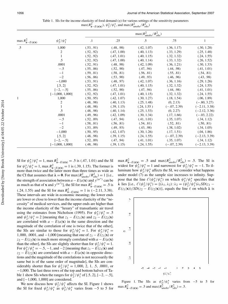
Table 1. SIs for the income elasticity of food demand (η) for various settings of the sensitivity parametersmax(R2

z−E(z|x)), ψ∗

2 /ψ∗1 , and max(R2

unobs/R2obs)

max(R2unobs/R

2obs)

maxR2z−E(z|x)

ψ∗2 /ψ∗

1 .1 .25 .5 .75 1

.5 1,000 (.53, .91) (.48, .98) (.42, 1.07) (.36, 1.17) (.30, 1.28)2 (.52, .92) (.47, 1.00) (.40, 1.13) (.33, 1.29) (.25, 1.48)1 (.52, .92) (.47, 1.01) (.40, 1.15) (.32, 1.32) (.24, 1.55).5 (.52, .92) (.47, 1.00) (.40, 1.14) (.33, 1.32) (.26, 1.52)

.0001 (.52, .91) (.48, .98) (.42, 1.09) (.36, 1.21) (.30, 1.33)−.5 (.55, .86) (.52, .90) (.47, .94) (.44, .98) (.41, 1.01)−1 (.59, .81) (.58, .81) (.56, .81) (.55, .81) (.54, .81)−2 (.56, .86) (.53, .90) (.49, .93) (.46, .96) (.43, .98)

−1,000 (.53, .91) (.48, .97) (.42, 1.07) (.36, 1.16) (.29, 1.26)[.5, 2] (.52, .92) (.47, 1.01) (.40, 1.15) (.32, 1.32) (.24, 1.55)

[−2, −.5] (.55, .86) (.52, .90) (.47, .94) (.44, .98) (.41, 1.01)[−1,000, 1,000] (.52, .92) (.47, 1.01) (.40, 1.15) (.32, 1.32) (.24, 1.55)

1 1,000 (.50, .95) (.42, 1.07) (.30, 1.27) (.18, 1.54) (.06, 1.89)2 (.48, .98) (.40, 1.13) (.25, 1.48) (0, 2.13) (−.80, 3.27)1 (.48, .98) (.39, 1.15) (.24, 1.55 ) (−.07, 2.39) (−2.11, 3.38).5 (.48, .98) (.40, 1.14) (.25, 1.53) (0, 2.27) (−2.12, 3.36)

.0001 (.49, .96) (.42, 1.09) (.30, 1.34) (.17, 1.66) (−.03, 2.22)−.5 (.52, .89) (.47, .94) (.41, 1.01) (.35, 1.07) (.34, 1.12)−1 (.58, .81) (.56, .81) (.54, .81) (.52, .81) (.50, .81)−2 (.53, .89) (.49, .93) (.43, .98) (.38, 1.02) (.34, 1.05)

−1,000 (.50, .95) (.42, 1.07) (.30, 1.26) (.17, 1.51) (.04, 1.86)[.5, 2] (.48, .98) (.39, 1.15) (.24, 1.55) (−.07, 2.39) (−2.13, 3.39)

[−2, −.5] (.52, .89) (.47, .94) (.41, 1.01) (.35, 1.07) (.34, 1.12)[−1,000, 1,000] (.48, .98) (.39, 1.15) (.24, 1.55) (−.07, 2.39) (−2.13, 3.39)

SI for ψ∗2 /ψ∗

1 = 1, maxR2z−E(z|x) = .5 is (.47,1.01) and the SI

for ψ∗2 /ψ∗

1 = 1, maxR2z−E(z|x) = 1 is (.39,1.15). The former is

more than twice and the latter more than three times as wide asthe CI that assumes that λ = 0. For max(R2

unobs/R2obs) = 1 [i.e.,

the strength of association between a−E(a|x) and y(w∗) can beas much as that of x and y(w∗)], the SI for maxR2

z−E(z|x) = .5 is

(.24,1.55) and the SI for maxR2z−E(z|x) = 1 is (−2.11,3.38).

These intervals are wide in economic meaning; the lower endsare lower or close to lower than the income elasticity of the “ne-cessity” of medical services, and the upper ends are higher thanthe income elasticity of the “luxury” of transatlantic air travelusing the estimates from Nicholson (1995). For ψ∗

2 /ψ∗1 = .5

and ψ∗2 /ψ∗

1 = 2 [meaning that z1 − E(z1|x) and z2 − E(z2|x)

are correlated with a − E(a|x) in the same direction and themagnitude of the correlation of one is twice that of the other],the SIs are similar to those for ψ∗

2 /ψ∗1 = 1. For ψ∗

2 /ψ∗1 =

1,000, .0001, and −1,000 [meaning that one of z1 −E(z1|x) orz2 −E(z2|x) is much more strongly correlated with a −E(a|x)

than the other], the SIs are slightly shorter than for ψ∗2 /ψ∗

1 = 1.For ψ∗

2 /ψ∗1 = −.5, −1, and −2 [meaning that z1 −E(z1|x) and

z2 − E(z2|x) are correlated with a − E(a|x) in opposite direc-tions and the magnitude of the correlations is not necessarily thesame but is of the same order of magnitude], the SIs are con-siderably shorter than for ψ∗

2 /ψ∗1 = 1,000, 2, 1, .5, .0001, or

−1,000. The last three rows of the top and bottom halves of Ta-ble 1 show SIs when the ranges for ψ∗

2 /ψ∗1 of [.5,2], [−2,−.5],

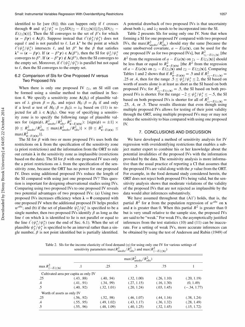
and [−1,000, 1,000] are considered.We now discuss how ψ∗

2 /ψ∗1 affects the SI. Figure 1 shows

the SI for fixed ψ∗2 /ψ∗

1 as ψ∗2 /ψ∗

1 varies from −5 to 5 for

maxR2z−E(z|x) = .5 and max(R2

unobs/R2obs) = .5. The SI is

widest for ψ∗2 /ψ∗

1 = 1 and narrowest for ψ∗2 /ψ∗

1 = −1. To il-luminate how ψ∗

2 /ψ∗1 affects the SI, we consider what happens

under model (7) as the sample size increases to infinity. Sup-pose that the line �′(ψ∗

2 /ψ∗1 ) on which ψ∗

2 /ψ∗1 specifies that

λ lies [i.e., �′(ψ∗2 /ψ∗

1 ) = {(λ1, λ2) :λ2 = (ψ∗2 /ψ∗

1 )λ1SD(z1 −E(z1|x))/SD(z2 − E(z2|x))}, equals the line � on which λ is

Figure 1. The SIs as ψ∗2 /ψ∗

1 varies from −5 to 5 for

maxR2z−E(z|x)

= .5 and max(R2unobs/R

2obs) = .5.

Dow

nloa

ded

by [

Ston

y B

rook

Uni

vers

ity]

at 0

4:05

22

Oct

ober

201

4

Small: Instrumental Variables Regression With Overidentifying Restrictions 1057

identified to lie [see (8)]; this can happen only if � crossesthrough 0 and ψ∗

2 /ψ∗1 = [γ2SD(z2 − E(z2|x))]/[γ1SD(z1 −

E(z1|x))]. Then the SI converges to the set of β’s for which(κ − βγ ) ∈ A(β). Suppose instead that �′(ψ∗

2 /ψ∗1 ) does not

equal � and is not parallel to �. Let λ∗ be the point at which�′(ψ∗

2 /ψ∗1 ) intersects �, and let β∗ be the β that satisfies

λ∗ = (κ − βγ ). If (κ − β∗γ ) ∈ A(β∗), then the SI for ψ∗2 /ψ∗

1converges to β∗. If (κ −β∗γ ) /∈ A(β∗), then the SI converges tothe empty set. Moreover, if �′(ψ∗

2 /ψ∗1 ) is parallel but not equal

to �, then the SI converges to the empty set.

6.2 Comparison of SIs for One Proposed IV versusTwo Proposed IVs

When there is only one proposed IV z1, an SI still canbe formed using a similar method to that outlined in Sec-tion 4. We specify a sensitivity zone A(β0) of plausible val-ues of λ given β = β0, and reject H0 :β = β0 if and onlyif a level α test of H0 :β = β0|λ = λ0 based on (11) is re-jected for all λ ∈ A(β0). One way of specifying a sensitiv-ity zone is to specify the following range of plausible val-ues for (sign(φ),R2

unobs/R2obs,R

2z−E(z|x)): {sign(φ) = ±1} ×

{0 ≤ R2unobs/R

2obs ≤ max(R2

unobs/R2obs)} × {0 ≤ R2

z−E(z|x) ≤max(R2

z−E(z|x))}.The SI for β with two or more proposed IVs uses both the

restrictions on λ from the specification of the sensitivity zone(a priori restrictions) and the information from the ORT to ruleout certain λ in the sensitivity zone as implausible (restrictionsbased on the data). The SI for β with one proposed IV uses onlythe a priori restrictions on λ from the specification of the sen-sitivity zone, because the ORT has no power for one proposedIV. Does using additional proposed IVs reduce the length ofthe SI compared with using just one proposed IV? This ques-tion is important for designing observational studies using IVs.Comparing using two proposed IVs to one proposed IV revealstwo potential advantages of two proposed IVs: (a) Using twoproposed IVs increases efficiency when λ = 0 compared withone proposed IV when the additional proposed IV helps predictwobs; and (b) if the set of plausible ψ∗

2 /ψ∗1 is specified to be a

single number, then two proposed IVs identify β as long as theline � on which λ is identified to lie is not parallel or equal tothe line �

′(ψ∗

1 /ψ∗2 ) (see the end of Sec. 6.1). When the set of

plausible ψ∗2 /ψ∗

1 is specified to be an interval rather than a sin-gle number, β is not point identified but is partially identified.

A potential drawback of two proposed IVs is that uncertaintyabout both λ1 and λ2 needs to be incorporated into the SI.

Table 2 presents SIs for using only one IV. Note that whenforming a SI for one proposed IV compared with two proposedIVs, the max(R2

unobs/R2obs) should stay the same [because the

same unobserved covariate, a − E(a|x), can be used for theone proposed IV as for two proposed IVs], but R2

z1−E(z1|x) [the

R2 from the regression of a − E(a|x) on z1 − E(z1|x)] shouldbe less than or equal to R2

z−E(z|x) [the R2 from the regressionof a − E(a|x) on z1 − E(z1|x) and z2 − E(z2|x)]. ComparingTables 1 and 2 shows that if R2

z−E(z|x)= .5 and if R2

z1−E(z1|x)=

.25 or .4, then for the range .5 ≤ ψ∗2 /ψ∗

1 ≤ 2, the SI based onworth of assets alone is at least as short as the SI based on bothproposed IVs; for R2

z1−E(z1|x)= .5, the SI based on both pro-

posed IVs is shorter. For the range −2 ≤ ψ∗2 /ψ∗

1 ≤ −.5, the SIbased on both proposed IVs is shorter for all of R2

z1−E(z1|x) =.25, .4, or .5. These results illustrate that even though usingmultiple proposed IVs allows for testing of their joint validitythrough the ORT, using multiple proposed IVs may or may notreduce the sensitivity to bias compared with using one proposedIV.

7. CONCLUSIONS AND DISCUSSION

We have developed a method of sensitivity analysis for IVregression with overidentifying restrictions that enables a sub-ject matter expert to combine his or her knowledge about thepotential invalidities of the proposed IVs with the informationprovided by the data. The sensitivity analysis is more informa-tive than the usual practice of reporting a CI that assumes thatthe proposed IVs are valid along with the p value from the ORT.For example, in the food demand study considered herein, theORT does not reject both proposed IVs being valid, but the sen-sitivity analysis shows that moderate violations of the validityof the proposed IVs that are not rejected as implausible by thedata would alter inferences substantively.

We have assumed throughout that (A1′) holds, that is, thepartial R2 for z from the population regression of wobs on xand z is greater than 0. When this partial R2 is greater than 0but is very small relative to the sample size, the proposed IVsare said to be “weak.” For weak IVs, the asymptotically justifiedinferences from the test statistics (10) and (11) can be inaccu-rate. For a setting of weak IVs, more accurate inferences canbe obtained by using the test of Anderson and Rubin (1949) of

Table 2. SIs for the income elasticity of food demand (η) for using only one IV for various settings ofsensitivity parameters max(R2

unobs/R2obs) and max(R2

z−E(z|x))

max(R2unobs/R

2obs)

maxR2z−E(z|x)

.1 .25 .5 .75 1

Cultivated area per capita as only IV.25 (.43, .88) (.40, .94) (.32, 1.00) (.26, 1.10) (.20, 1.19).4 (.41, .91) (.34, .99) (.27, 1.15) (.16, 1.30) (0, 1.49).5 (.40, .92) (.32, 1.01) (.20, 1.24) (.03, 1.45) (−.34, 1.77)

Worth of assets as only IV.25 (.56, .92) (.52, .98) (.46, 1.07) (.44, 1.16) (.38, 1.24).4 (.55, .95) (.49, 1.02) (.43, 1.17) (.36, 1.32) (.28, 1.49).5 (.55, .96) (.48, 1.09) (.40, 1.25) (.32, 1.45) (.15, 1.72)

Dow

nloa

ded

by [

Ston

y B

rook

Uni

vers

ity]

at 0

4:05

22

Oct

ober

201

4

1058 Journal of the American Statistical Association, September 2007

H0 :β = β0,λ = λ0 or other tests described by Stock, Wright,and Yogo (2002). However, for the food demand study, the IVsare not weak so that using inferences based on (10) and (11)is reasonable. Stock et al. considered two IVs to be weak if theF -statistic for testing that the coefficients on z in the populationregression of wobs on x and z are both 0 is <11.59 (see Table 1of Stock et al. 2002); this F statistic for the food demand studyis 306.3, much larger than 11.59.

[Received September 2005. Revised March 2007.]

REFERENCES

Anderson, T. W., and Rubin, H. (1949), “Estimation of the Parameters of Coef-ficients of a Single Equation in a Simultaneous System and Their AsymptoticExpansions,” Econometrica, 41, 683–714.

Angrist, J., and Imbens, G. (1995), “Estimation of Average Causal Effects,”Journal of the American Statistical Association, 90, 431–442.

Angrist, J. D., Imbens, G. W., and Rubin, D. R. (1996), “Identification of CausalEffects Using Instrumental Variables,” Journal of the American StatisticalAssociation, 91, 444–472.

Bardhan, P., and Udry, C. (1999), Development Microeconomics, New York:Oxford University Press.

Bouis, H. E., and Haddad, L. J. (1990), “Effects of Agricultural Commercial-ization on Land Tenure, Household Resource Allocation, and Nutrition in thePhilippines,” Research Report 79, IFPRI, Boulder, CO: Lynne Rienner Pub-lishers.

Card, D. (1995), “Using Geographic Variation in College Proximity to Esti-mate the Return to Schooling,” in Aspects of Labour Market Behaviour, eds.L. Christofides, E. Grant, and R. Swidinsky, Toronto: University of TorontoPress, pp. 201–222.

Davidson, R., and MacKinnon, J. (1993), Estimation and Inference in Econo-metrics, New York: Oxford University Press.

Hall, A. R. (2005), Generalized Method of Moments, New York: Oxford Uni-versity Press.

Hansen, L. P. (1982), “Large-Sample Properties of Generalized Method-of-Moments Estimators,” Econometrica, 50, 1029–1054.

Hausman, J. A. (1983), “Specification and Estimation of Simultaneous Equa-tion Models,” in Handbook of Econometrics, Vol. 1, eds. Z. Griliches andM. D. Intriligator, Amsterdam: North-Holland, pp. 391–448.

Holland, P. W. (1988), “Causal Inference, Path Analysis and Recursive Struc-tural Equation Models,” Sociological Methodology, 18, 449–484.

Imbens, G. W. (2003), “Sensitivity to Exogeneity Assumptions in ProgramEvaluation,” The American Economic Review, 93, 126–132.

Kadane, J. B., and Anderson, T. W. (1977), “A Comment on the Test of Overi-dentifying Restrictions,” Econometrica, 45, 1027–1032.

Kane, T., and Rouse, C. (1993), “Labor Market Returns to Two- and Four-YearColleges: Is a Credit a Credit and Do Degrees Matter?” Working Paper 4268,National Bureau of Economic Research.

Manski, C. (1995), Identification Problems in the Social Sciences, Cambridge,MA: Harvard University Press.

Newey, W.K. (1985), “Generalized Method-of-Moments Specification Test-ing,” Journal of Econometrics, 29, 229–256.

Neyman, J. (1923), “On the Application of Probability Theory to Agricul-tural Experiments,” translated by D. Dabrowska, Statistical Science (1990),5, 463–480.

Nicholson, W. (1995), Microeconomic Theory (6th ed.), New York: Harcourt.Rosenbaum, P. R. (1986), “Dropping out of High School in the United States,”

Journal of Educational and Behavioral Statistics, 11, 207–224.(1999), “Using Combined Quantile Averages in Matched Observa-

tional Studies,” Applied Statistics, 48, 63–78.(2002), Observational Studies (2nd. ed.), New York: Springer-Verlag.

Rothenberg, T. J. (1971), “Identification in Parametric Models,” Econometrica,39, 577–591.

Rubin, D. B. (1974), “Estimating Causal Effects of Treatments in Random-ized and Non-Randomized Studies,” Journal of Educational Psychology, 66,688–701.

(1978), “Bayesian Inference for Causal Effects: The Role of Random-ization,” The Annals of Statistics, 6, 34–58.

(1986), “Statistics and Causal Inference: Comment: Which ifs HaveCausal Answers,” Journal of the American Statistical Association, 81,961–962.

Sargan, J. D. (1958), “The Estimation of Economic Relationships Using Instru-mental Variables,” Econometrica, 26, 393–415.

Stock, J. H., Wright, J. H., and Yogo, M. (2002), “A Survey of Weak Instru-ments and Weak Identification in Generalized Method of Moments,” Journalof Business & Economic Statistics, 20, 518–529.

Tan, Z. (2006), “Regression and Weighting Methods for Causal Inference UsingInstrumental Variables,” Journal of the American Statistical Association, 101,1607–1618.

White, H. (1982), “Instrumental Variables Regression With Independent Ob-servations,” Econometrica, 50, 483–500.

Wooldridge, J. M. (1997), “On Two-Stage Least Squares Estimation of the Av-erage Treatment Effect in a Random Coefficient Model,” Economics Letters,56, 129–133.

Zheng, X., and Loh, W.-Y. (1995), “Consistent Variable Selection in LinearModels,” Journal of the American Statistical Association, 90, 151–156.

Dow

nloa

ded

by [

Ston

y B

rook

Uni

vers

ity]

at 0

4:05

22

Oct

ober

201

4