Sensible heat flux in high winds
23
AMTD 5, 447–469, 2012 Sensible heat flux in high winds S. P. Burns et al. Title Page Abstract Introduction Conclusions References Tables Figures Back Close Full Screen / Esc Printer-friendly Version Interactive Discussion Discussion Paper | Discussion Paper | Discussion Paper | Discussion Paper | Atmos. Meas. Tech. Discuss., 5, 447–469, 2012 www.atmos-meas-tech-discuss.net/5/447/2012/ doi:10.5194/amtd-5-447-2012 © Author(s) 2012. CC Attribution 3.0 License. Atmospheric Measurement Techniques Discussions This discussion paper is/has been under review for the journal Atmospheric Measurement Techniques (AMT). Please refer to the corresponding final paper in AMT if available. Using sonic anemometer temperature to measure sensible heat flux in strong winds S. P. Burns 1,2 , T. W. Horst 1 , P. D. Blanken 2 , and R. K. Monson 3 1 National Center for Atmospheric Research, Boulder, Colorado, USA 2 Department of Geography, University of Colorado, Boulder, USA 3 School of Natural Resources and the Environment, University of Arizona, Tucson, USA Received: 2 December 2011 – Accepted: 3 January 2012 – Published: 12 January 2012 Correspondence to: S. P. Burns ([email protected]) Published by Copernicus Publications on behalf of the European Geosciences Union. 447
Transcript of Sensible heat flux in high winds

AMTD5, 447–469, 2012
Sensible heat flux inhigh winds
S. P. Burns et al.
Title Page
Abstract Introduction
Conclusions References
Tables Figures
J I
J I
Back Close
Full Screen / Esc
Printer-friendly Version
Interactive Discussion
Discussion
Paper
|D
iscussionP
aper|
Discussion
Paper
|D
iscussionP
aper|
Atmos. Meas. Tech. Discuss., 5, 447–469, 2012www.atmos-meas-tech-discuss.net/5/447/2012/doi:10.5194/amtd-5-447-2012© Author(s) 2012. CC Attribution 3.0 License.
AtmosphericMeasurement
TechniquesDiscussions
This discussion paper is/has been under review for the journal Atmospheric MeasurementTechniques (AMT). Please refer to the corresponding final paper in AMT if available.
Using sonic anemometer temperature tomeasure sensible heat flux in strongwindsS. P. Burns1,2, T. W. Horst1, P. D. Blanken2, and R. K. Monson3
1National Center for Atmospheric Research, Boulder, Colorado, USA2Department of Geography, University of Colorado, Boulder, USA3School of Natural Resources and the Environment, University of Arizona, Tucson, USA
Received: 2 December 2011 – Accepted: 3 January 2012 – Published: 12 January 2012
Correspondence to: S. P. Burns ([email protected])
Published by Copernicus Publications on behalf of the European Geosciences Union.
447
AMTD5, 447–469, 2012
Sensible heat flux inhigh winds
S. P. Burns et al.
Title Page
Abstract Introduction
Conclusions References
Tables Figures
J I
J I
Back Close
Full Screen / Esc
Printer-friendly Version
Interactive Discussion
Discussion
Paper
|D
iscussionP
aper|
Discussion
Paper
|D
iscussionP
aper|
Abstract
The sensible heat flux (H) is a significant component of the surface energy balance(SEB). Sonic anemometers simultaneously measure the turbulent fluctuations of ver-tical wind (w ′) and sonic temperature (T ′
s), and are commonly used to measure H .Our study examines 30-min heat fluxes measured with a Campbell Scientific model5
CSAT3 sonic anemometer above a subalpine forest. We compare H calculated with Tsto H calculated with a co-located thermocouple and find that for horizontal wind speed(U) less than 8 m s−1 the agreement is ≈± 30 W m−2. However, for U >≈8 m s−1, theCSAT3 H becomes larger than H calculated with the thermocouple, reaching a max-imum difference of ≈250 W m−2 at U ≈18 m s−1. H calculated with the thermocouple10
results in a SEB that is relatively independent of U at high wind speeds. In contrast,the SEB calculated with H from the CSAT3 varies considerably with U , particularly at
night. Cospectral analysis of w ′T ′s suggest that spurious correlation is a problem dur-
ing high winds which leads to a positive (additive) increase in H calculated with theCSAT3. At night, when H is typically negative, this CSAT3 error results in a measured15
H that falsely approaches zero or even becomes positive. Within a broader context,the usefulness of side-by-side instrument comparisons are discussed.
1 Introduction
Sonic anemometers have been used to measure three-dimensional wind vectors, tem-perature, and surface sensible heat and momentum fluxes since the early 1960s. They20
have played a pivotal role in studying the surface energy balance (SEB), which de-scribes how the radiative energy at the earth’s surface is partitioned between latentheat flux (evaporation and transpiration of water to the atmosphere) and sensible heatflux (heat exchange between the surface elements, ground, and atmosphere) (Stew-art and Thom, 1973; Garratt, 1992; Blanken et al., 1997; Oncley et al., 2007; Foken,25
2008). Despite improvements in instrumentation accuracy, most flux-measuring sites
448
AMTD5, 447–469, 2012
Sensible heat flux inhigh winds
S. P. Burns et al.
Title Page
Abstract Introduction
Conclusions References
Tables Figures
J I
J I
Back Close
Full Screen / Esc
Printer-friendly Version
Interactive Discussion
Discussion
Paper
|D
iscussionP
aper|
Discussion
Paper
|D
iscussionP
aper|
find that the measured sensible and latent heat fluxes only account for ≈80 % of theavailable incoming energy (Wilson et al., 2002; Foken, 2008). The so-called “energybalance closure problem” has recently been reviewed (Foken, 2008; Foken et al., 2011)and the conclusion was reached that the imbalance can be mostly attributed to low-frequency flux contributions from heterogenous landscapes which are not measured5
by eddy-covariance techniques. The energy balance closure typically improves un-der windy/turbulent conditions when the ground and atmosphere are “well-coupled”(Franssen et al., 2010). Spatially homogeneous and moisture-limited environmentssuch as deserts appear to be optimal for successfully closing the energy budget (Tim-ouk et al., 2009; Foken, 2008).10
This paper uses data from the Niwot Ridge Subalpine Forest AmeriFlux site (NWT)to examine the sensible heat flux with strong winds. Turnipseed et al. (2002) studiedthe energy balance at the NWT site and found that during the daytime the sum of theturbulent fluxes accounts for 80–90 % of the radiative energy input into the forest. Atnight, under moderately turbulent conditions, the energy balance closure is comparable15
to the daytime. However, when the nighttime conditions are either calm or extremelyturbulent, the sensible and latent heat fluxes only account for 20-60 % of the net long-wave radiative flux. Turnipseed et al. (2002) discussed several possible reasons forthis nighttime discrepancy (e.g., instrument error, footprint mis-match, horizontal ad-vection), but none of these reasons could adequately explain the fact that the nighttime20
imbalance persisted in the presence of strong winds. They concluded that the sonictemperature did not have sufficient resolution to capture the small temperature fluctua-tions which led to inaccurate sensible heat fluxes.
In early 2008 the sonic anemometers at NWT were re-calibrated (details in Sect. 2.3).After the recalibration, the new sensible heat flux still did not improve the agreement25
between the daytime and nocturnal energy balance in windy conditions, and the imbal-ance was even more dramatic than before the re-calibration. The goals of the currentstudy are to: (1) describe the discrepancy observed in the calculated sensible heat flux,(2) compare the sensible heat flux calculated using sonic temperature to that calculated
449
AMTD5, 447–469, 2012
Sensible heat flux inhigh winds
S. P. Burns et al.
Title Page
Abstract Introduction
Conclusions References
Tables Figures
J I
J I
Back Close
Full Screen / Esc
Printer-friendly Version
Interactive Discussion
Discussion
Paper
|D
iscussionP
aper|
Discussion
Paper
|D
iscussionP
aper|
with a co-located thermocouple, and (3) re-visit the surface energy balance results fromTurnipseed et al. (2002) in light of the results from item (2).
2 Data and methods
2.1 Site description
This study uses data from the Niwot Ridge Subalpine Forest AmeriFlux site (40◦1′58′′ N,5
105◦32′47′′ W, 3050 m elevation, data version 2011.04.20). The site is located be-low Niwot Ridge, Colorado, 8 km east of the Continental Divide. The NWT measure-ments started in November 1998 as described in Monson et al. (2002) and Turnipseedet al. (2002, 2003). The tree density around the NWT Tower is ≈0.4 trees m−2 witha leaf area index (LAI) of 3.8–4.2 m2 m−2 and tree heights of 12–13 m (Turnipseed10
et al., 2002). In winter, NWT is a windy place. Between November–February, the 30-min average 21.5 m wind speed (U) is around 7 m s−1 (standard deviation ≈4.5 m s−1)with a maximum U near 20 m s−1. More information on NWT is available on-line athttp://public.ornl.gov/ameriflux/.
2.2 Sonic anemometer thermometry15
A few of the important relationships related to sonic anemometer thermometry aresummarized here; a more complete description of the technology is readily available(e.g., Kaimal and Businger, 1963; Schotanus et al., 1983; Kaimal and Gaynor, 1991;Loescher et al., 2005, and many others).
A sonic anemometer-thermometer calculates air temperature (T ) by measuring the20
speed of sound (c). The relationship between air temperature, the speed of sound,and specific humidity (q) within the atmosphere is well-known,
T =c2
γd Rd
(1
1 + 0.51q
), (1)
450
AMTD5, 447–469, 2012
Sensible heat flux inhigh winds
S. P. Burns et al.
Title Page
Abstract Introduction
Conclusions References
Tables Figures
J I
J I
Back Close
Full Screen / Esc
Printer-friendly Version
Interactive Discussion
Discussion
Paper
|D
iscussionP
aper|
Discussion
Paper
|D
iscussionP
aper|
where γd =cp/cv =1.4 is the dry air specific heat ratio and Rd is the gas constant for
dry air (287.04 J kg−1 K−1).A sonic anemometer-thermometer sequentially transmits and receives sound pulses
between two transducers separated by a path-length distance (d ). The sonic tempera-ture (Ts) is determined from the measured times to transit d (t1 in one direction and t25
in the opposite direction) and the geometry of the sound rays such that,
Ts ≡ c2
γd Rd=
1γd Rd
[(d2
)2 (1t1
+1t2
)2
+ V 2n
], (2)
where Vn is the wind component perpendicular to d (i.e., cross-wind). Equation (2) isfor dry air.
In a real atmosphere (i.e., one with water vapor), air temperature is calculated from10
Ts as T airs = Ts (1+0.51q)−1. If the measured variables are decomposed into mean and
fluctuating components (e.g., T = T + T ′, etc., see Schotanus et al., 1983), then thesensible heat flux H is calculated with,
H = ρ cp w ′T ′ = ρ cp
[w ′T ′
s − 0.51 T w ′q′ + 2T u
c2u′w ′
], (3)
where ρ is the air density, cp is the specific heat of air at constant pressure, and u and15
w are the horizontal and vertical wind components in streamwise coordinates. The u′w ′
term is the so-called cross-wind correction term and most modern sonic anemometerstake this into account with internal processing software (Loescher et al., 2005; Camp-bell Scientific, 2011).
2.3 Energy balance equation and instrumentation20
The terms in the surface energy balance are,
Ra = Rnet − G − Scanopy − Ssoil = H + LE, (4)451
AMTD5, 447–469, 2012
Sensible heat flux inhigh winds
S. P. Burns et al.
Title Page
Abstract Introduction
Conclusions References
Tables Figures
J I
J I
Back Close
Full Screen / Esc
Printer-friendly Version
Interactive Discussion
Discussion
Paper
|D
iscussionP
aper|
Discussion
Paper
|D
iscussionP
aper|
where Ra is the “available energy”. At NWT, net radiation (Rnet) was measured atz≈25 m above the ground with both a net (Radiation and Energy Balance Systems –REBS, model Q*7.1) and four-component (Kipp and Zonen, model CNR-1) radiometer.The soil heat flux (G) was measured with multiple soil heat flux plates (REBS, ModelHFT-1) at a depth of −10 cm. The two storage terms (Scanopy and Ssoil) account for the5
heat stored between the ground and the flux measurement heights, and are typicallyless than 10 % of Rnet (Oncley et al., 2007). At NWT, Turnipseed et al. (2002) showedthat the storage terms and G were small (less than 8 % of Rnet) and we neglect Scanopyand Ssoil for this study.
Latent heat flux (LE), and H were measured at z≈21.5 m with a Campbell Scientific10
model CSAT3 sonic anemometer (hereafter “CSAT”; Campbell Scientific, 2011) pro-viding the high-frequency vertical wind (w ′) and temperature (T ′
s) fluctuations, whilewater vapor (q′) was measured with a co-located krypton hygrometer (Turnipseedet al., 2002). Winds are rotated from sonic to planar-fit coordinates prior to the fluxcalculations (Wilczak et al., 2001). Ts output by a CSAT is an average from three non-15
orthogonal paths. We use “HCSAT” to designate H calculated with Ts following Eq. (3). Inour discussions, SEB refers to the ratio of the sum of the turbulent fluxes to (Rnet −G),i.e., SEB= (H +LE)/(Rnet −G).
The CSAT can operate with either embedded code version 3 or version 4 (hereafter,ver3 and ver4) and uses advanced digital signal processing to determine the ultrasonic20
times of flight (e.g., t1 and t2 in Eq. 2). Ver4 is designed to produce usable resultswhen the signal is weak such as when liquid water is on the transducers, but degradesthe Ts resolution from 0.002 ◦C in ver3 to 0.03 ◦C in ver4 (see Campbell Scientific, 2011for more details about ver3 versus ver4).
Here, we briefly summarize the sequence of events that led to our study (also see25
Table 1). In 2008 we sent the three University of Colorado (CU) CSATs (all ver3) backto Campbell Scientific, Inc. for re-calibration and one of them (sn 0328) was upgradedto ver4. After deploying the ver4 CU CSAT at 21.5 m, we observed nighttime HCSATvalues that were frequently above zero, indicating heat was being transported from
452
AMTD5, 447–469, 2012
Sensible heat flux inhigh winds
S. P. Burns et al.
Title Page
Abstract Introduction
Conclusions References
Tables Figures
J I
J I
Back Close
Full Screen / Esc
Printer-friendly Version
Interactive Discussion
Discussion
Paper
|D
iscussionP
aper|
Discussion
Paper
|D
iscussionP
aper|
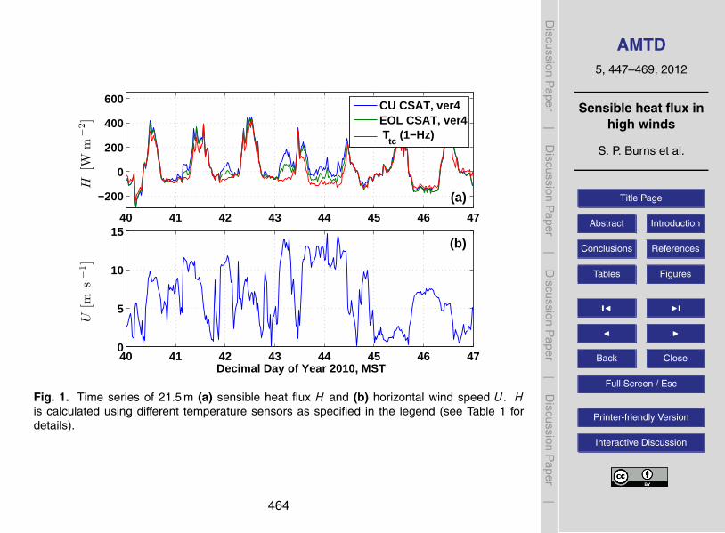
the surface to the atmosphere at night. Though such conditions are possible for shortperiods (e.g., due to warm air advection), we have rarely observed such phenomenain the previous 10 years of measurements. These anomalous HCSAT measurementswere strongly correlated with high winds (Fig. 1).
Because we were curious/suspicious about these above-zero nighttime HCSAT val-5
ues, we deployed a CSAT from the National Center for Atmospheric Research (NCAR)Earth Observing Laboratory (EOL) at the same level as the CU CSAT (ver4). TheEOL CSAT initially used ver3, which we changed to ver4 partway through our study(Table 1). To change from ver3 to ver4, the processing chip in the CSAT electronics en-closure was changed, but the sonic head was not disturbed. Additional air temperature10
information was provided near the 21.5 m level by a 0.254 mm E-type thermocouplethat was located about 1.4 m from the CU CSAT and sampled at 1-Hz. Because wewere concerned about flux loss due to horizontal separation and lack of high-frequencysampling, a second E-type thermocouple was deployed in May 2010 within 5 cm of theCU CSAT transducers and sampled at 10-Hz. The thermocouple temperature fluc-15
tuations (T ′tc) are correlated with w ′ from the CU CSAT to calculate a sensible heat
flux (e.g., HTtc = ρcpw ′T ′tc). The other temperature sensor at the 21.5 m level was a
mechanically-aspirated slow-response temperature-humidity sensor (Vaisala HMP35-D probe) which we use as a “reference” sensor for time-averaged comparisons.
3 Results and discussion20
3.1 Comparison of sensible heat fluxes
If H is calculated using the EOL CSAT, CU CSAT, and Ttc there are large H differencesduring periods of strong winds that are most obvious at night (Fig. 1). In a perfectsonic anemometer the path-length d is constant, however real world changes to dcan occur as the sensor material expands and contracts due to temperature changes25
or wind-induced stresses or vibrations. Lanzinger and Langmack (2005) use a Thies
453

AMTD5, 447–469, 2012
Sensible heat flux inhigh winds
S. P. Burns et al.
Title Page
Abstract Introduction
Conclusions References
Tables Figures
J I
J I
Back Close
Full Screen / Esc
Printer-friendly Version
Interactive Discussion
Discussion
Paper
|D
iscussionP
aper|
Discussion
Paper
|D
iscussionP
aper|
two-dimensional sonic anemometer to show that a 50 K temperature change resultsin a 0.4 mm change in d which produces a 1.2 K error in Ts. We did not observe anytemperature-dependent H differences in our study.
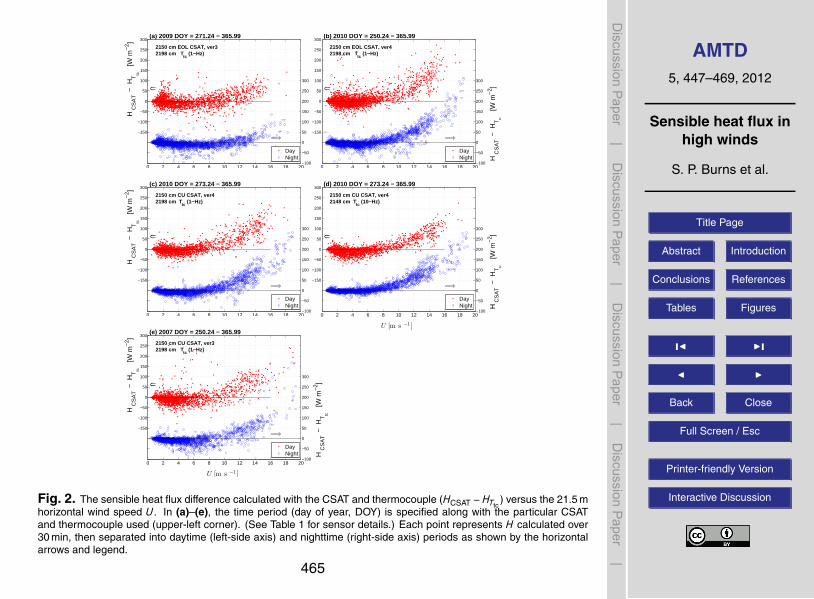
After separating the H data by day and night, there is a consistent trend in theHCSAT −HTtc
difference; for U >≈8 m s−1, HCSAT becomes more positive than HTtcand5
the difference increases as U increases up to a difference of ≈250 W m−2 at U ≈17 m s−1
(Fig. 2). Our original supposition that this was primarily a nighttime problem is incorrectbecause the daytime and nighttime differences are qualitatively similar. We have sepa-rated the panels of Fig. 2 into periods when different configurations of CSATs were onthe tower (Table 1). By comparing Fig. 2a and 2b we find that HCSAT EOL ver3 agreed10
better with HTtcthan HCSAT EOL ver4. Also, HCSAT −HTtc
for EOL CSAT ver3 did nothave as strong a dependence on U as ver4.
One issue of concern with HTtc(1-Hz) is the ≈1.4 m horizontal sensor separation be-
tween the CU CSAT (w ′) and 1-Hz thermocouple (T ′tc) (Horst and Lenschow, 2009). If
one compares HCSAT −HTtcusing Ttc 1-Hz (Fig. 2c) with Ttc 10-Hz (Fig. 2d), the trend15
of increasing H difference with increasing U is apparent for both thermocouples. Thisencourages us that H calculated with Ttc (1-Hz) results in a viable heat flux; further-more, as one would expect, HTtc
(10-Hz) has reduced scatter in HCSAT −HTtc. Though
HTtc(1-Hz) and HTtc
(10-Hz) appear similar, there are some differences between themwhich are discussed below. We should note that it would be useful to confirm that Ttc20
(10-Hz) is adequately capturing the high-frequency (f >≈2 Hz) portion of w ′T ′tc. How-
ever, a visual comparison with previously published w ′T ′ cospectra (e.g., Kaimal andFinnigan, 1994; Blanken et al., 1998; Massman and Clement, 2005) suggest that ourresults are reasonable.
In order to make a connection to the older heat flux data (e.g., data collected between25
1998–2008), we examine CU CSAT ver3 HCSAT −HTtc(1-Hz) from a period prior to the
CSAT recalibration (Fig. 2e). The dependence of HCSAT −HTtcon U is similar to that
observed with the other CSATs. This result is important in our consideration of the
454

AMTD5, 447–469, 2012
Sensible heat flux inhigh winds
S. P. Burns et al.
Title Page
Abstract Introduction
Conclusions References
Tables Figures
J I
J I
Back Close
Full Screen / Esc
Printer-friendly Version
Interactive Discussion
Discussion
Paper
|D
iscussionP
aper|
Discussion
Paper
|D
iscussionP
aper|
energy budget (Sect. 3.2) and to make a link to the results from Turnipseed et al.(2002).
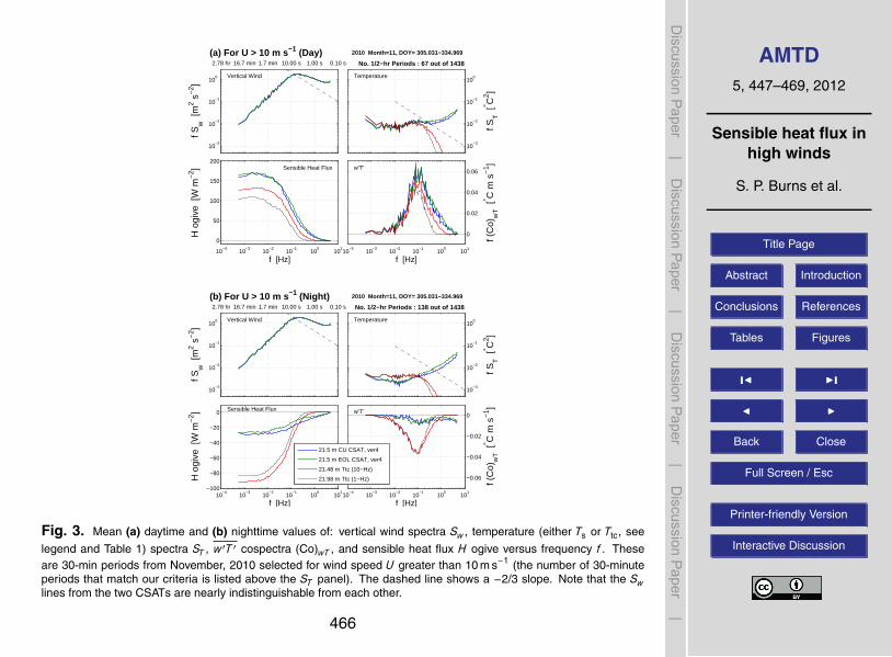
To gain further insight into the HCSAT −HTtcdifferences, we examine the spectra of w ′,
T ′s, and T ′
tc and their associated cospectra and ogives (Friehe et al., 1991) for high-windconditions (Fig. 3). The Sw and ST spectra from the two CSATs are in good agreement,5
but show the effect of high-frequency noise and aliasing. ST from Ttc (10-Hz) is attenu-ated at frequencies above ≈1 Hz because the thermal mass of the thermocouple wirelimits the response time. In high-wind conditions (e.g., when the Sw and ST energy peakis shifted to higher frequencies) we observe that HTtc
(1-Hz) is about 10–20 % smallerthan HTtc
(10-Hz) due to the lower sampling rate as well as the horizontal separation.10
During the day the low-frequency part of ST and (Co)wT for the CSAT and thermocoupleare in fairly good agreement (Fig. 3a). At night, however, ST from Ttc has more energythan Ts, and (Co)wTtc
differs dramatically from the cospectra of the two CSATs. The
H ogive reveals nocturnal HTtc≈−90 W m−2 compared to HCSAT ≈−30 W m−2 (Fig. 3b).
It appears there is spurious correlation in w ′T ′s that enhances (Co)wTs
during the day15
and degrades it at night. As U becomes smaller, the spectra and cospectra come intobetter agreement (Fig. 4).
We considered the possibility of tower/sonic vibration or movement affecting the tran-
sit times (e.g., t1 and t2 in Eq. 2) and causing the w ′T ′s error. However, the main source
of the problem appears to be with T ′s not w ′ because w ′T ′
tc, which uses the same CSAT20
w ′, produces reasonable heat fluxes, e.g., predominantly negative H at night. Also,similar high-frequency noise in CSAT ST (not shown here) have been observed on a30-m tower during high-winds in the CHATS field project (Patton et al., 2011). Thissuggests the problem is not specific to the NWT tower. Furthermore, discussions withCampbell Scientific, Inc. engineers have also led us to believe that sensor movement25
is not the cause of the problem. Without an independent measure of w ′ it is difficult tocheck the vertical wind, but we note that Sw in high winds is flatter than the expected−2/3 slope (Fig. 3a–b). Finally, we also considered the w ′q′ and u′w ′ terms in Eq. (3),
455
AMTD5, 447–469, 2012
Sensible heat flux inhigh winds
S. P. Burns et al.
Title Page
Abstract Introduction
Conclusions References
Tables Figures
J I
J I
Back Close
Full Screen / Esc
Printer-friendly Version
Interactive Discussion
Discussion
Paper
|D
iscussionP
aper|
Discussion
Paper
|D
iscussionP
aper|
but found them too small to explain the discrepancy between HCSAT and HTtc(results
not shown).In order to look further at the possibility of errors in Ts, we compare T air
s and Ttc toan aspirated temperature-humidity sensor (Tasp) as a function of U . At night (Fig. 5aand b), the Ttc − Tasp difference is less than ±0.1 ◦C and independent of U . However,5
during the day (Fig. 5c and d) there is a well-known radiation effect on Ttc that causesit to be larger than Tasp by about 0.6 ◦C at low wind speeds but decreases to 0.2 ◦C for
high winds (e.g., Campbell, 1969; Burns and Sun, 2000). It is also well-known that T airs
can contain a significant bias relative to true T due to uncertainties in the sonic pathlength (Loescher et al., 2005). Therefore, we adjust T air
s with a linear fit to Tasp (the10
coefficients of the fit are listed in Fig. 5).From Fig. 5 it can be seen that, during both day and night and for ver3 and ver4
CSATs, T airs shows a systematic decrease on the order of 0.2 ◦C as U increases from
around 8 to 15 m s−1. This negative T airs error correlated with increasing U explains the
positive HCSAT error in the NWT data. Since w ′ is negatively correlated with u′ in the15
surface layer and the T ′s error is also negatively correlated with u′, the w ′T ′
s error ispositive, as observed.
3.2 Consideration of the surface energy balance
As mentioned in the introduction, Turnipseed et al. (2002) found that the nocturnal SEBclosure during high winds varied between 0.2–0.6. In Fig. 6, the SEB is calculated us-20
ing HCSAT (CU ver3) and HTtc(1-Hz). As one would expect, the SEB with HCSAT (CU
ver3) closely matches the results of Turnipseed et al. (2002). At night (Fig. 6b), theSEB peaks at ≈0.7 for moderate U , and then becomes negative as U increases (or asfriction velocity u∗ increases as shown in Fig. 7 of Turnipseed et al., 2002). Also similarto Turnipseed et al. (2002), we find the nocturnal SEB with Rnet from the Q*7.1 sensor25
is about 15 % closer to closing the SEB than with the CNR-1 sensor. For low winds,drainage flows form at the NWT site (Yi et al., 2005; Burns et al., 2011) and result in
456
AMTD5, 447–469, 2012
Sensible heat flux inhigh winds
S. P. Burns et al.
Title Page
Abstract Introduction
Conclusions References
Tables Figures
J I
J I
Back Close
Full Screen / Esc
Printer-friendly Version
Interactive Discussion
Discussion
Paper
|D
iscussionP
aper|
Discussion
Paper
|D
iscussionP
aper|
near-zero nocturnal SEB values due to decoupling, strong horizontal advection of tem-perature, and practical difficulties with the flux calculation (e.g., Mahrt, 2010). Theselow-wind conditions require knowledge of horizontal advection for a more completeunderstanding (Sun et al., 2007; Yi et al., 2008).
During the day (Fig. 6a), the SEB using HTtcand HCSAT diverge at U ≈6 m s−1. For5
U >13 m s−1, the SEB with HCSAT is close to 1. Knowing about the HCSAT error in highwinds (e.g., as discussed in Sect. 3.1 and shown in Fig. 3a) suggests that the daytimeSEB approaching 1 is an artifact. In contrast, with HTtc
, both the daytime and nighttime
SEB values for U >6 m s−1 are in reasonable agreement at SEB≈0.65–0.75, and thereis almost no dependence of the SEB on U . Unless there is a physical reason for the10
SEB to change with higher wind speeds, using HTtcappears more reasonable than
HCSAT. If true, SEB closure at NWT without considering the storage terms is around70 %. Taking into account the storage terms in Eq. (4) and the slight underestimationof HTtc
(1-Hz) we would expect the SEB closure to improve by about 10–15 %.
To better estimate the magnitude (in W m−2) of the SEB deficit we consider the15
2006–2008 mean nocturnal values of Rnet from the CNR-1 (≈−85 W m−2) and Q*7.1(≈−60 W m−2) sensors. This difference of 25 W m−2 results in a 15 % difference in theSEB (Fig. 6b). These two Rnet sensors are known to be accurate to only 20 W m−2
(Brotzge and Duchon, 2000; Foken, 2008; Michel et al., 2008) and within complex ter-rain radiation measurements are complicated (Oliphant et al., 2003). This suggests20
that a “field-calibration” of the current radiation sensors to a high-accuracy radiometer(e.g., Burns et al., 2003) could improve our understanding of the surface energy budgetat the site, and possibly, help explain the remaining lack of closure. Other factors thatmight cause the lack of closure are discussed elsewhere (e.g., Turnipseed et al., 2002;Foken, 2008; Foken et al., 2011).25
457

AMTD5, 447–469, 2012
Sensible heat flux inhigh winds
S. P. Burns et al.
Title Page
Abstract Introduction
Conclusions References
Tables Figures
J I
J I
Back Close
Full Screen / Esc
Printer-friendly Version
Interactive Discussion
Discussion
Paper
|D
iscussionP
aper|
Discussion
Paper
|D
iscussionP
aper|
4 Conclusions
We compared H calculated using sonic anemometer temperature to H calculated with aco-located thermocouple and found U-dependent H differences on the order of 250 W m−2
at high wind speeds. To better understand these H differences, we considered the sur-face energy budget. Using HTtc
, the daytime and nighttime SEB values for U >6 m s−15
were fairly consistent (between 0.65–0.75). In contrast, using HCSAT the SEB values instrong winds vary from below 0 (at night) to around 1 (during the day). Because thereis no physical explanation for the wide variation in SEB with HCSAT, we conclude that Hcalculated with the thermocouple is more reasonable. From analysis of the spectra andco-spectra of w ′T ′ in high winds, we conclude there is spurious correlation between w ′
10
and T ′s that lead to positive increases in HCSAT. At night H is typically negative, and,
for strong winds, the w ′T ′s correlation error makes the magnitude of nocturnal HCSAT
smaller than it should be. Because Ttc and Ts are both correlated with w ′ from thesame CSAT, we conclude that Ts is the primary source of the error.
We have been in contact with Campbell Scientific, Inc. regarding our observed heat15
flux discrepancies. They subsequently performed their own independent experimentsto confirm the sonic temperature issues we have presented. Their preliminary resultswith a CSAT ver4 indicate that the issue occurs at all wind speeds, but is significantfor U >8 m s−1. Campbell Scientific, Inc. is currently working to better quantify themagnitude of the error and will mitigate it with future hardware and/or software changes.20
Though our study examines one specific model of sonic anemometer, the tests wehave outlined with a thermocouple could (and should) be used with any field-deployedsonic anemometer. Furthermore, in a broader context, our temperature comparisonshows the added value of independent, co-located, in-situ measurements in environ-mental research. Previous comparisons of sonic anemometers by Loescher et al.25
(2005) were very thorough, but performed the comparison up to a wind speed of≈6 m s−1 so any issues at higher wind speeds were undetected. This emphasizesan important advantage of long-term in-situ comparisons – they cover the range of the
458

AMTD5, 447–469, 2012
Sensible heat flux inhigh winds
S. P. Burns et al.
Title Page
Abstract Introduction
Conclusions References
Tables Figures
J I
J I
Back Close
Full Screen / Esc
Printer-friendly Version
Interactive Discussion
Discussion
Paper
|D
iscussionP
aper|
Discussion
Paper
|D
iscussionP
aper|
observation. In short, our study provides a practical example of how valuable in-situcomparisons can be in evaluating sensor performance.
Acknowledgements. We gratefully acknowledge assistance from the scientists and staff atCampbell Scientific, Inc., especially Ed Swiatek and Larry Jacobsen for their support and in-terest. Don Lenschow, Gordon Maclean, and Steve Oncley provided useful discussions. We5
also thank Chris Golubieski for assistance with the EOL CSAT. The NWT tower is supportedby a grant from the National Science Foundation (NSF) Long-Term Research in EnvironmentalBiology (LTREB). The National Center for Atmospheric Research (NCAR) is sponsored by NSF.
References
Blanken, P. D., Black, T. A., Yang, P. C., Neumann, H. H., Nesic, Z., Staebler, R., den Hartog,10
G., Novak, M. D., and Lee, X.: Energy balance and canopy conductance of a boreal aspenforest: Partitioning overstory and understory components, J. Geophys. Res.-Atmos., 102,28915–28927, 1997. 448
Blanken, P. D., Black, T. A., Neumann, H. H., Den Hartog, G., Yang, P. C., Nesic, Z., Staebler,R., Chen, W., and Novak, M. D.: Turbulent flux measurements above and below the overstory15
of a boreal aspen forest, Bound.-Lay. Meteorol., 89, 109–140, 1998. 454Brotzge, J. A. and Duchon, C. E.: A Field Comparison among a Domeless Net Radiometer,
Two Four-Component Net Radiometers, and a Domed Net Radiometer, J. Atmos. Ocean.Tech., 17, 1569–1582, doi:10.1175/1520-0426(2000)017<1569:AFCAAD>2.0.CO;2, 2000.45720
Burns, S. P. and Sun, J.: Thermocouple temperature measurements from the CASES-99 maintower, in: 14th Symposium on Boundary Layer and Turbulence, Amer. Meteor. Soc., Snow-mass, Colorado, 358–361, 2000. 456
Burns, S. P., Sun, J., Delany, A. C., Semmer, S. R., Oncley, S. P., and Horst, T. W.: A fieldintercomparison technique to improve the relative accuracy of longwave radiation measure-25
ments and an evaluation of CASES-99 pyrgeometer data quality, J. Atmos. Ocean. Tech.,20, 348–361, doi:10.1175/1520-0426(2003)020<0348:AFITTI>2.0.CO;2, 2003. 457
459
AMTD5, 447–469, 2012
Sensible heat flux inhigh winds
S. P. Burns et al.
Title Page
Abstract Introduction
Conclusions References
Tables Figures
J I
J I
Back Close
Full Screen / Esc
Printer-friendly Version
Interactive Discussion
Discussion
Paper
|D
iscussionP
aper|
Discussion
Paper
|D
iscussionP
aper|
Burns, S. P., Sun, J., Lenschow, D. H., Oncley, S. P., Stephens, B. B., Chuixiang, Y., Anderson,D. E., Hu, J., and Monson, R. K.: Atmospheric stability effects on wind fields and scalarmixing within and just above a subalpine forest in sloping terrain, Bound.-Lay. Meteorol.,138, 231–262, doi:10.1007/s10546-010-9560-6, 2011. 456
Campbell, G. S.: Measurement of air temperature fluctuations with thermocouples,5
Tech. Rep. ECOM-5273, Atmospheric Sciences Laboratory, White Sands Missile Range,10 pp., 1969. 456
Campbell Scientific: CSAT3 Three Dimensional Sonic Anemometer Manual (Revision 10/11),available at: www.campbellsci.com, last access: 10 January 2012, Campbell Scientific, Inc.,Logan, Utah, 70 pp., 2011. 451, 45210
Foken, T.: The energy balance closure problem: An overview, Ecol. Appl., 18, 1351–1367,2008. 448, 449, 457
Foken, T., Aubinet, M., Finnigan, J. J., Leclerc, M. Y., Mauder, M., and Paw U, K. T.: Resultsof a panel discussion about the energy balance closure correction for trace gases, B. Am.Meteorol. Soc., 92, ES13–ES18, 2011. 449, 45715
Franssen, H. J. H., Stockli, R., Lehner, I., Rotenberg, E., and Seneviratne, S. I.: Energy balanceclosure of eddy-covariance data: A multisite analysis for European FLUXNET stations, Agr.Forest Meteorol., 150, 1553–1567, doi:10.1016/j.agrformet.2010.08.005, 2010. 449
Friehe, C. A., Shaw, W. J., Rogers, D. P., Davidson, K. L., Large, W. G., Stage, S. A., Crescenti,G. H., Khalsa, S. J. S., Greenhut, G. K., and Li, F.: Air-sea fluxes and surface-layer turbulence20
around a sea-surface temperature front, J. Geophys. Res., 96, 8593–8609, 1991. 455Garratt, J. R.: The atmospheric boundary layer, Cambridge University Press, Cambridge,
316 pp., 1992. 448Horst, T. W. and Lenschow, D. H.: Attenuation of Scalar Fluxes Measured with Spatially-
displaced Sensors, Bound.-Lay. Meteorol., 130, 275–300, 2009. 45425
Kaimal, J. C. and Businger, J. A.: A continuous wave sonic anemometer-thermometer, J. Appl.Meteorol., 2, 156–164, 1963. 450
Kaimal, J. C. and Finnigan, J. J.: Atmospheric boundary layer flows: their structure and mea-surement, Oxford University Press, New York, 289 pp., 1994. 454
Kaimal, J. C. and Gaynor, J. E.: Another look at sonic thermometry, Bound.-Lay. Meteorol., 56,30
401–410, 1991. 450
460

AMTD5, 447–469, 2012
Sensible heat flux inhigh winds
S. P. Burns et al.
Title Page
Abstract Introduction
Conclusions References
Tables Figures
J I
J I
Back Close
Full Screen / Esc
Printer-friendly Version
Interactive Discussion
Discussion
Paper
|D
iscussionP
aper|
Discussion
Paper
|D
iscussionP
aper|
Lanzinger, E. and Langmack, H.: Measuring Air Temperature by using an UltrasonicAnemometer, in: Technical Conference on Meteorological and Environmental Instru-ments and Methods of Observation (TECO-2005), WMO Tech. Doc. No. 1265; IOM Re-port No. 82, http://www.wmo.int/pages/prog/www/IMOP/publications/IOM-82-TECO 2005/Programme index.html last access: 10 January 2012, World Meteorological Organization,5
Geneva, Switzerland, p.P3(9), 2005. 453Loescher, H. W., Ocheltree, T., Tanner, B., Swiatek, E., Dano, B., Wong, J., Zimmerman, G.,
Campbell, J., Stock, C., Jacobsen, L., Shiga, Y., Kollas, J., Liburdy, J., and Law, B. E.:Comparison of temperature and wind statistics in contrasting environments among differentsonic anemometer-thermometers, Agr. Forest Meteorol., 133, 119–139, 2005. 450, 451,10
456, 458Mahrt, L.: Computing turbulent fluxes near the surface: needed improvements, Agr. Forest
Meteorol., 150, 501–509, 2010. 457Massman, W. and Clement, R.: Uncertainty in Eddy Covariance Flux Estimates Resulting from
Spectral Attenuation, in: Handbook of Micrometeorology, edited by: Lee, X., Massman, W.,15
and Law, B., vol. 29 of Atmospheric and Oceanographic Sciences Library, Springer, TheNetherlands, 67–99, 2005. 454
Michel, D., Philipona, R., Ruckstuhl, C., Vogt, R., and Vuilleumier, L.: Performance and un-certainty of CNR1 net radiometers during a one-year field comparison, J. Atmos. Ocean.Technol., 25, 442–451, 2008. 45720
Monson, R. K., Turnipseed, A. A., Sparks, J. P., Harley, P. C., Scott-Denton, L. E., Sparks,K., and Huxman, T. E.: Carbon sequestration in a high-elevation, subalpine forest, GlobalChange Biol., 8, 459–478, 2002. 450
Oliphant, A. J., Spronken-Smith, R. A., Sturman, A. P., and Owens, I. F.: Spatial variability ofsurface radiation fluxes in mountainous terrain, J. Appl. Meteorol., 42, 113–128, 2003. 45725
Oncley, S. P., Foken, T., Vogt, R., Kohsiek, W., DeBruin, H. A. R., Bernhofer, C., Christen, A.,van Gorsel, E., Grantz, D., Feigenwinter, C., Lehner, I., Liebethal, C., Liu, H., Mauder, M.,Pitacco, A., Ribeiro, L., and Weidinger, T.: The Energy Balance Experiment EBEX-2000,Part I: Overview and energy balance, Bound.-Lay. Meteorol., 123, 1–28, 2007. 448, 452
Patton, E. G., Horst, T. W., Sullivan, P. P., Lenschow, D. H., Oncley, S. P., Brown, W. O. J.,30
Burns, S. P., Guenther, A. B., Held, A., Karl, T., Mayor, S. D., Rizzo, L. V., Spuler, S. M.,Sun, J., Turnipseed, A. A., Allwine, E. J., Edburg, S. L., Lamb, B. K., Avissar, R., Calhoun,R. J., Kleissl, J., Massman, W. J., Paw, K. T., and Weil, J. C.: The Canopy Horizontal Array
461
AMTD5, 447–469, 2012
Sensible heat flux inhigh winds
S. P. Burns et al.
Title Page
Abstract Introduction
Conclusions References
Tables Figures
J I
J I
Back Close
Full Screen / Esc
Printer-friendly Version
Interactive Discussion
Discussion
Paper
|D
iscussionP
aper|
Discussion
Paper
|D
iscussionP
aper|
Turbulence Study, B. Am. Meteorol. Soc., 92, 593–611, 2011. 455Schotanus, P., Nieuwstadt, F. T. M., and De Bruin, H. A. R.: Temperature-measurement with
a sonic anemometer and its application to heat and moisture fluxes, Bound.-Lay. Meteorol.,26, 81–93, 1983. 450, 451
Stewart, J. B. and Thom, A. S.: Energy budgets in pine forest, Q. J. Roy. Meteorol. Soc., 99,5
154–170, 1973. 448Sun, J., Burns, S. P., Delany, A. C., Oncley, S. P., Turnipseed, A. A., Stephens, B. B., Lenschow,
D. H., LeMone, M. A., Monson, R. K., and Anderson, D. E.: CO2 transport over complexterrain, Agr. Forest Meteorol., 145, 1–21, doi:10.1016/j.agrformet.2007.02.007, 2007. 457
Timouk, F., Kergoat, L., Mougin, E., Lloyd, C. R., Ceschia, E., Cohard, J. M., de Rosnay, P.,10
Hiernaux, P., Demarez, V., and Taylor, C. M.: Response of surface energy balance to waterregime and vegetation development in a Sahelian landscape, J. Hydrol., 375, 178–189, 2009.449
Turnipseed, A. A., Blanken, P. D., Anderson, D. E., and Monson, R. K.: Energy budget above ahigh-elevation subalpine forest in complex topography, Agr. Forest Meteorol., 110, 177–201,15
2002. 449, 450, 452, 455, 456, 457, 469Turnipseed, A. A., Anderson, D. E., Blanken, P. D., Baugh, W. M., and Monson, R. K.: Airflows
and turbulent flux measurements in mountainous terrain. Part 1: canopy and local effects,Agr. Forest Meteorol., 119, 1–21, 2003. 450
Wilczak, J. M., Oncley, S. P., and Stage, S. A.: Sonic anemometer tilt correction algorithms,20
Bound.-Lay. Meteorol, 99, 127–150, 2001. 452Wilson, K., Goldstein, A., Falge, E., Aubinet, M., Baldocchi, D., Berbigier, P., Bernhofer, C.,
Ceulemans, R., Dolman, H., Field, C., Grelle, A., Ibrom, A., Law, B. E., Kowalski, A., Meyers,T., Moncrieff, J., Monson, R., Oechel, W., Tenhunen, J., Valentini, R., and Verma, S.: Energybalance closure at FLUXNET sites, Agr. Forest Meteorol., 113, 223–243, 2002. 44925
Yi, C., Monson, R. K., Zhai, Z. Q., Anderson, D. E., Lamb, B., Allwine, G., Turnipseed,A. A., and Burns, S. P.: Modeling and measuring the nocturnal drainage flow in ahigh-elevation, subalpine forest with complex terrain, J. Geophys. Res., 110, D22303,doi:10.1029/2005JD006282, 2005. 456
Yi, C., Anderson, D. E., Turnipseed, A. A., Burns, S. P., Sparks, J. P., Stannard, D. I., and30
Monson, R. K.: The contribution of advective fluxes to net ecosystem exchange in a high-elevation, subalpine forest, Ecol. Appl., 18, 1379–1390, doi:10.1890/06-0908.1, 2008. 457
462
AMTD5, 447–469, 2012
Sensible heat flux inhigh winds
S. P. Burns et al.
Title Page
Abstract Introduction
Conclusions References
Tables Figures
J I
J I
Back Close
Full Screen / Esc
Printer-friendly Version
Interactive Discussion
Discussion
Paper
|D
iscussionP
aper|
Discussion
Paper
|D
iscussionP
aper|
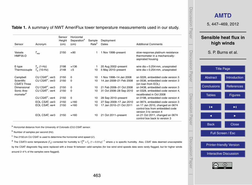
Table 1. A summary of NWT AmeriFlux tower temperature measurements used in our study.
Sensor HorizontalHeight Separationa Sample Deployment
Sensor Acronym (cm) (cm) Rateb Dates Additional Comments
Vaisala Tasp 2150 ≈90 1 1 Nov 1998–present slow-response platinum resistanceHMP35-D thermometer in a mechanically-
aspirated housing
E-type Ttc (1-Hz) 2198 ≈136 1 20 Aug 2002–present wire dia=0.254 mm, unaspiratedThermocouple Ttc (10-Hz) 2148 <5 10 5 May 2010–present wire dia=0.254 mm, unaspirated
Campbell CU CSATc, ver3 2150 0 10 1 Nov 1998–14 Jan 2008 sn 0226, embedded code version 3Scientific CU CSATc, ver3 2150 0 10 14 Jan 2008–21 Feb 2008 sn 0536, embedded code version 3CSAT3 Three (on loan from EOL)Dimensional CU CSATc, ver3 2150 0 10 21 Feb 2008–31 Oct 2008 sn 0438, embedded code version 3Sonic Ane- CU CSATc, ver4 2150 0 10 31 Oct 2008–28 Sep 2010 sn 0328, embedded code version 4,mometerd recalibrated in Oct 2008
CU CSATc, ver4 2150 0 10 28 Sep 2010–present sn 0198, embedded code version 4
EOL CSAT, ver3 2150 ≈160 10 27 Sep 2009–17 Jan 2010 sn 0674, embedded code version 3EOL CSAT, ver4 2150 ≈160 10 17 Jan 2010–21 Oct 2011 on 17 Jan 2010, changed sn 0674
control box from embedded codeversion 3 to version 4
EOL CSAT, ver3 2150 ≈160 10 21 Oct 2011–present on 21 Oct 2011, changed sn 0674control box back to version 3
a Horizontal distance from the University of Colorado (CU) CSAT sensor.
b Number of samples per second (Hz).
c The 2150 cm CU CSAT is used to determine the horizontal wind speed (U).
d The CSAT3 sonic temperature (Ts) corrected for humidity is T airs = Ts (1+0.51q)−1 where q is specific humidity. Also, CSAT data deemed unacceptable
by the CSAT diagnostic flag were replaced with a linear fit between valid samples (for low wind wind speeds data were rarely flagged, but for higher winds
around 2–4 % of the samples were flagged).
463
AMTD5, 447–469, 2012
Sensible heat flux inhigh winds
S. P. Burns et al.
Title Page
Abstract Introduction
Conclusions References
Tables Figures
J I
J I
Back Close
Full Screen / Esc
Printer-friendly Version
Interactive Discussion
Discussion
Paper
|D
iscussionP
aper|
Discussion
Paper
|D
iscussionP
aper|
40 41 42 43 44 45 46 47
−200
0
200
400
600
H
[Wm
−2]
(a)
CU CSAT, ver4EOL CSAT, ver4 T
tc (1−Hz)
40 41 42 43 44 45 46 470
5
10
15
Decimal Day of Year 2010, MST
U[m
s−
1]
(b)
Fig. 1. Time series of 21.5 m (a) sensible heat flux H and (b) horizontal wind speed U . His calculated using different temperature sensors as specified in the legend (see Table 1 fordetails).
464
AMTD5, 447–469, 2012
Sensible heat flux inhigh winds
S. P. Burns et al.
Title Page
Abstract Introduction
Conclusions References
Tables Figures
J I
J I
Back Close
Full Screen / Esc
Printer-friendly Version
Interactive Discussion
Discussion
Paper
|D
iscussionP
aper|
Discussion
Paper
|D
iscussionP
aper|
0 2 4 6 8 10 12 14 16 18 20
−100
−50
0
−150 50
−100 100
−50 150
0 200
50 250
100 300
150
200
250
300
H C
SA
T − H
Ttc
[W
m−
2 ]=⇒
⇐=
2150 cm EOL CSAT, ver32198 cm T
tc (1−Hz)
(a) 2009 DOY = 271.24 − 365.99
DayNight
0 2 4 6 8 10 12 14 16 18 20
−100
−50
0
−150 50
−100 100
−50 150
0 200
50 250
100 300
150
200
250
300
H C
SA
T − H
Ttc
[W
m−
2 ]
=⇒
⇐=
2150 cm EOL CSAT, ver42198 cm T
tc (1−Hz)
(b) 2010 DOY = 250.24 − 365.99
DayNight
0 2 4 6 8 10 12 14 16 18 20−100
−50
0
−150 50
−100 100
−50 150
0 200
50 250
100 300
150
200
250
300
H C
SA
T − H
Ttc
[W
m−
2 ]
=⇒
⇐=
2150 cm CU CSAT, ver42198 cm T
tc (1−Hz)
(c) 2010 DOY = 273.24 − 365.99
DayNight
0 2 4 6 8 10 12 14 16 18 20−100
−50
0
−150 50
−100 100
−50 150
0 200
50 250
100 300
150
200
250
300
H C
SA
T − H
Ttc
[W
m−
2 ]
U [m s −1 ]
=⇒
⇐=
2150 cm CU CSAT, ver42148 cm T
tc (10−Hz)
(d) 2010 DOY = 273.24 − 365.99
DayNight
0 2 4 6 8 10 12 14 16 18 20−100
−50
0
−150 50
−100 100
−50 150
0 200
50 250
100 300
150
200
250
300
H C
SA
T − H
Ttc
[W
m−
2 ]
H C
SA
T − H
Ttc
[W
m−
2 ]
U [m s −1 ]
=⇒
⇐=
2150 cm CU CSAT, ver32198 cm T
tc (1−Hz)
(e) 2007 DOY = 250.24 − 365.99
DayNight
Fig. 2. The sensible heat flux difference calculated with the CSAT and thermocouple (HCSAT −HTtc) versus the 21.5 m
horizontal wind speed U . In (a)–(e), the time period (day of year, DOY) is specified along with the particular CSATand thermocouple used (upper-left corner). (See Table 1 for sensor details.) Each point represents H calculated over30 min, then separated into daytime (left-side axis) and nighttime (right-side axis) periods as shown by the horizontalarrows and legend.
465
AMTD5, 447–469, 2012
Sensible heat flux inhigh winds
S. P. Burns et al.
Title Page
Abstract Introduction
Conclusions References
Tables Figures
J I
J I
Back Close
Full Screen / Esc
Printer-friendly Version
Interactive Discussion
Discussion
Paper
|D
iscussionP
aper|
Discussion
Paper
|D
iscussionP
aper|
10−3
10−2
10−1
100
f Sw [
m2 s
−2 ]
Vertical Wind
(a) For U > 10 m s−1 (Day)2.78 hr 16.7 min 1.7 min 10.00 s 1.00 s 0.10 s
10−3
10−2
10−1
100Temperature
f ST [
° C2 ]
2010 Month=11, DOY= 305.031−334.969
No. 1/2−hr Periods : 67 out of 1438
10−4
10−3
10−2
10−1
100
101
0
0.02
0.04
0.06w’T’
f (C
o)w
T [
° C m
s−
1 ]
f [Hz]10
−410
−310
−210
−110
010
1
0
50
100
150
200Sensible Heat Flux
H o
give
[W
m−
2 ]
f [Hz]
10−3
10−2
10−1
100
f Sw [
m2 s
−2 ]
Vertical Wind
(b) For U > 10 m s−1 (Night)2.78 hr 16.7 min 1.7 min 10.00 s 1.00 s 0.10 s
10−3
10−2
10−1
100Temperature
f ST [
° C2 ]
2010 Month=11, DOY= 305.031−334.969
No. 1/2−hr Periods : 138 out of 1438
10−4
10−3
10−2
10−1
100
101
−0.06
−0.04
−0.02
0w’T’
f (C
o)w
T [
° C m
s−
1 ]
f [Hz]10
−410
−310
−210
−110
010
1−100
−80
−60
−40
−20
0Sensible Heat Flux
H o
give
[W
m−
2 ]
f [Hz]
21.5 m CU CSAT, ver4
21.5 m EOL CSAT, ver4
21.48 m Ttc (10−Hz)
21.98 m Ttc (1−Hz)
Fig. 3. Mean (a) daytime and (b) nighttime values of: vertical wind spectra Sw , temperature (either Ts or Ttc, see
legend and Table 1) spectra ST , w ′T ′ cospectra (Co)wT , and sensible heat flux H ogive versus frequency f . Theseare 30-min periods from November, 2010 selected for wind speed U greater than 10 m s−1 (the number of 30-minuteperiods that match our criteria is listed above the ST panel). The dashed line shows a −2/3 slope. Note that the Swlines from the two CSATs are nearly indistinguishable from each other.
466

AMTD5, 447–469, 2012
Sensible heat flux inhigh winds
S. P. Burns et al.
Title Page
Abstract Introduction
Conclusions References
Tables Figures
J I
J I
Back Close
Full Screen / Esc
Printer-friendly Version
Interactive Discussion
Discussion
Paper
|D
iscussionP
aper|
Discussion
Paper
|D
iscussionP
aper|
10−4
10−3
10−2
10−1
100
101
−0.01
0
0.01
0.02
0.03
0.04w’T’
f (C
o)w
T [
° C m
s−
1 ]
f [Hz]
For 6 m s −1 < U < 10 m s−1 (Day)
10−3
10−2
10−1
Temperature
f ST [
° C2 ]
2010 Month=11, DOY= 305.031−334.969
No. 1/2−hr Periods : 81 out of 1438
f [Hz]
10−4
10−3
10−2
10−1
100
101
−0.04
−0.03
−0.02
−0.01
0
0.01w’T’
f (C
o)w
T [
° C m
s−
1 ]
f [Hz]
For 6 m s −1 < U < 10 m s−1 (Night)
10−3
10−2
10−1
Temperature
f ST [
° C2 ]
2010 Month=11, DOY= 305.031−334.969
No. 1/2−hr Periods : 203 out of 1438
f [Hz]
10−4
10−3
10−2
10−1
100
101
−0.01
0
0.01
0.02
0.03
0.04w’T’
f (C
o)w
T [
° C m
s−
1 ]
f [Hz]
For U < 6 m s−1 (Day)
10−3
10−2
10−1
Temperature
f ST [
° C2 ]
2010 Month=11, DOY= 305.031−334.969
No. 1/2−hr Periods : 336 out of 1438
f [Hz]
10−4
10−3
10−2
10−1
100
101
−0.04
−0.03
−0.02
−0.01
0
0.01w’T’
f (C
o)w
T [
° C m
s−
1 ]
f [Hz]
For U < 6 m s−1 (Night)
10−3
10−2
10−1
Temperature
f ST [
° C2 ]
2010 Month=11, DOY= 305.031−334.969
No. 1/2−hr Periods : 402 out of 1438
f [Hz]
Fig. 4. The (left column) w ′T ′ cospectra (Co)wT and (right column) temperature spectra ST formedium- and low-wind conditions (see Fig. 3 for the legend and further details).
467

AMTD5, 447–469, 2012
Sensible heat flux inhigh winds
S. P. Burns et al.
Title Page
Abstract Introduction
Conclusions References
Tables Figures
J I
J I
Back Close
Full Screen / Esc
Printer-friendly Version
Interactive Discussion
Discussion
Paper
|D
iscussionP
aper|
Discussion
Paper
|D
iscussionP
aper|
0 2 4 6 8 10 12 14 16 18
−0.2
0
0.2
0.4
0.6
0.8 Sensor Gain Offset
CU CSAT 0.990 0.310
T−
Tasp
[◦C
]
(a) 2007, DOY = 1.01 − 365.70, Nighttime Data
T airs
, CU CSAT, ver3
Ttc
(1−Hz)
0 2 4 6 8 10 12 14 16 18
−0.2
0
0.2
0.4
0.6
0.8 Sensor Gain Offset
CU CSAT 1.000 −0.071
EOL CSAT 1.007 −0.194
(b) 2010, DOY = 17.70 − 365.70, Nighttime Data
T airs
, CU CSAT, ver4
T airs
, EOL CSAT, ver4
Ttc
(1−Hz)
0 2 4 6 8 10 12 14 16 18
−0.2
0
0.2
0.4
0.6
0.8 Sensor Gain Offset
CU CSAT 0.990 0.403
T−
Tasp
[◦C
]
U [m s −1 ]
(c) 2007, DOY = 1.39 − 365.64, Daytime Data
T airs
, CU CSAT, ver3
Ttc
(1−Hz)
0 2 4 6 8 10 12 14 16 18
−0.2
0
0.2
0.4
0.6
0.8 Sensor Gain Offset
CU CSAT 1.005 0.149
EOL CSAT 1.011 −0.042
U [m s −1 ]
(d) 2010, DOY = 17.53 − 365.66, Daytime Data
T airs
, CU CSAT, ver4
T airs
, EOL CSAT, ver4
Ttc
(1−Hz)
Fig. 5. The (a, b) nighttime and (c, d) daytime mean temperature difference (T − Tasp) versus21.5 m horizontal wind speed U . Tasp is measured within a mechanically-aspirated housing and
T is from either the humidity-corrected CSATs (T airs ) or a thermocouple (Ttc, 1-Hz) as specified
in the legend (also see Table 1). T airs has been linearly adjusted to Tasp using the gain and offset
shown in the upper left corner of each panel. The time period (day of year, DOY) used for eachpanel is shown.
468

AMTD5, 447–469, 2012
Sensible heat flux inhigh winds
S. P. Burns et al.
Title Page
Abstract Introduction
Conclusions References
Tables Figures
J I
J I
Back Close
Full Screen / Esc
Printer-friendly Version
Interactive Discussion
Discussion
Paper
|D
iscussionP
aper|
Discussion
Paper
|D
iscussionP
aper|
0 2 4 6 8 10 12 14 16−0.2
−0.1
0
0.1
0.2
0.3
0.4
0.5
0.6
0.7
0.8
0.9
1
1.1
(a) Day
(H
+L
E)/R
a
CU CSAT (ver3), CNR−1CU CSAT (ver3), Q*7.1Ttc (1−Hz), CNR−1Ttc (1−Hz), Q*7.1
0 2 4 6 8 10 12 14 16−0.2
−0.1
0
0.1
0.2
0.3
0.4
0.5
0.6
0.7
0.8
0.9
1
1.1
(b) Night
U [m s−1]
(H
+L
E)/R
a
Fig. 6. The surface energy balance [SEB= (H +LE)/Ra] versus horizontal wind speed U fromyears 2006–2008 for (a) daytime and (b) nighttime conditions (Ra =Rnet −G is the availableenergy, see text for details). The sensors used to calculate H (CU CSAT, ver3 or Ttc, 1-Hz) andRnet (Kipp and Zonen, model CNR-1 or REBS, model Q*7.1) are specified in the legend. (Thisfigure is comparable to Fig. 7 in Turnipseed et al., 2002.)
469