Senior Research PREDICTING THE RESULT OF …efriedma/research/boldrin.pdf1.1 Soccer in England ......

Senior Research

PREDICTING THE RESULT OF ENGLISH PREMIER LEAGUE SOCCER GAMES WITH

THE USE OF POISSON MODELS

By

Brianne Boldrin

Primary Advisor: Dr. Rasp

Secondary Advisor: Dr. Friedman

A SENIOR RESEARCH PAPER PRESENTED TO THE DEPARTMENT OF

MATHEMATICS AND COMPUTER SCIENCE OF STETSON UNIVERSITY IN PARTIAL

FULFILLMENT OF THE REQUIREMENTS FOR THE DEGREE OF BACHELOR OF

SCIENCE

STETSON UNIVERSITY

2017

2

ACKNOWLEDGEMENTS

I would like to thank my primary advisor, Dr. Rasp for the support, knowledge and guidance that

he has provided me throughout my research. I would also like to thank my secondary advisor,

Dr. Friedman, for his support and advice on my research efforts.

3

TABLE OF CONTENTS

Acknowledgements .........................................................................................................................2

List of Tables ...................................................................................................................................5

List of Figures ..................................................................................................................................6

Abstract ............................................................................................................................................7

Sections:

1. Literature Review.........................................................................................................................7

1.1 Soccer in England ...................................................................................................................7

1.2 Soccer Statistics ......................................................................................................................8

1.3 Modeling Match Outcomes ....................................................................................................9

1.4 Goal Scoring .........................................................................................................................10

1.4.1 Probability Distribution of Goals Scored ......................................................................10

1.4.2 Poisson Distribution ......................................................................................................11

1.4.3 Distribution Application ................................................................................................13

1.5 Variable Analysis .................................................................................................................16

2. Game Results Model Application ..............................................................................................17

2.1 Data Selection ......................................................................................................................18

2.2 Model Creation and Calculation ..........................................................................................20

2.2.1 Model 1 – Simple Poisson Distribution Model with Independent Teams ...................21

2.2.2 Model 2 – Poisson Distribution Assuming Dependence .............................................24

2.2.3 Model 3 – Multi-Variable Poisson Distribution with Home/ Away Factor .................27

2.3 Model Evaluation with Test Data .........................................................................................30

2.3.1 Code Automation ........................................................................................................30

2.3.2 Expanded Data Analysis .............................................................................................32

2.3.3 Amount of Previous Data .............................................................................................35

3. Betting Model Application ......................................................................................................37

3.1 Betting Odds .........................................................................................................................37

3.1.1 Types of Odds ..............................................................................................................38

3.2 Expected Profit Betting Model………………..……………………………………...........41

3.2.1 Expected Profit ............................................................................................................41

3.2.2 Automated Betting Code ..............................................................................................42

4

3.2.3 Betting Results .......................................................................................................43

3.3 Team Potential Profitability Betting Model …………………………………….…...........47

3.3.1 Selected Bet ................................................................................................................47

3.3.2 Team Potential Profitability Betting Results ................................................................48

4. Results ........................................................................................................................................51

5. Future Research .........................................................................................................................56

5.1 Derived Maximum Likelihood Estimator…………………………………........................56

5.2 Model Enhancements ...........................................................................................................58

References ......................................................................................................................................61

Code Appendix……..……………………………………………………………………………63

5

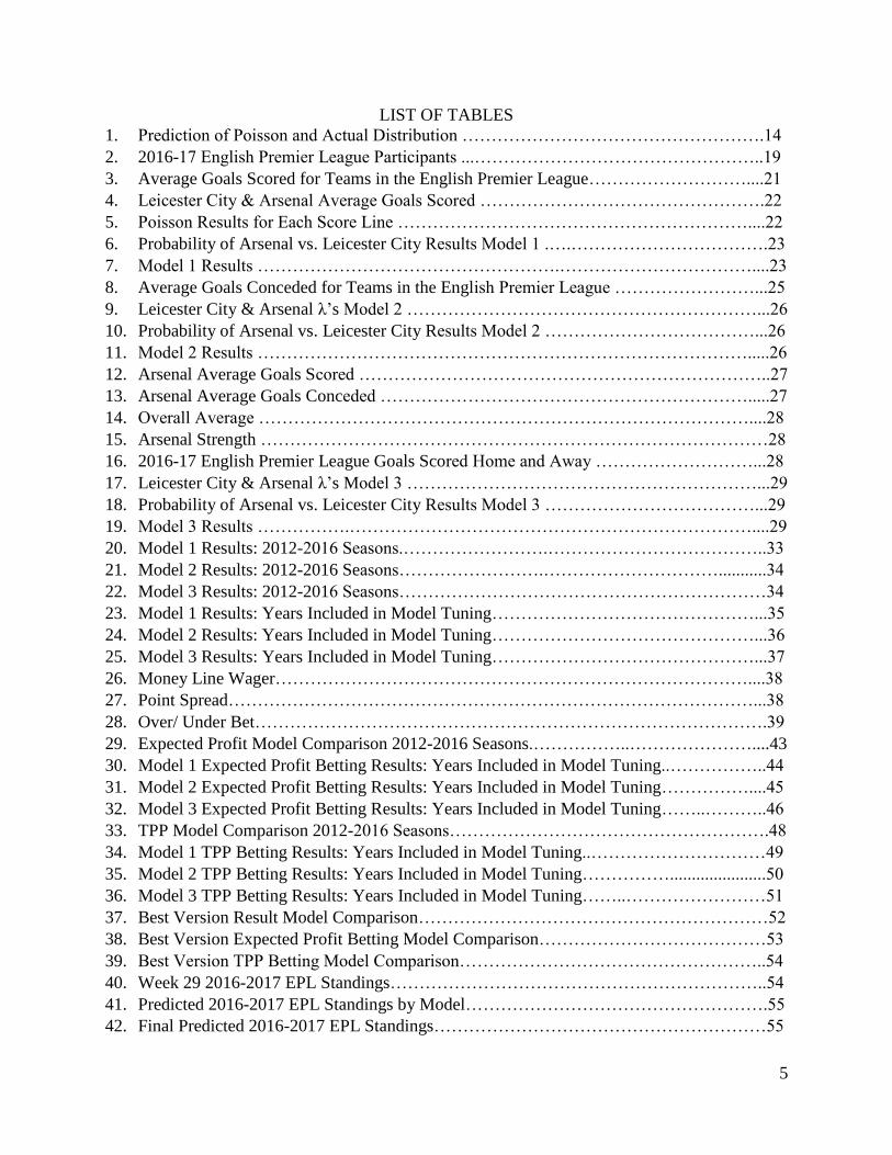
LIST OF TABLES

1. Prediction of Poisson and Actual Distribution …………………………………………….14

2. 2016-17 English Premier League Participants ...…………………………………………..19

3. Average Goals Scored for Teams in the English Premier League………………………....21

4. Leicester City & Arsenal Average Goals Scored ………………………………………….22

5. Poisson Results for Each Score Line ……………………………………………………....22

6. Probability of Arsenal vs. Leicester City Results Model 1 .….…………………………….23

7. Model 1 Results …………………………………………….……………………………....23

8. Average Goals Conceded for Teams in the English Premier League ……………………...25

9. Leicester City & Arsenal λ’s Model 2 ……………………………………………………...26

10. Probability of Arsenal vs. Leicester City Results Model 2 ………………………………...26

11. Model 2 Results ………………………………………………………………………….....26

12. Arsenal Average Goals Scored ……………………………………………………………..27

13. Arsenal Average Goals Conceded ……………………………………………………….....27

14. Overall Average …………………………………………………………………………....28

15. Arsenal Strength ……………………………………………………………………………28

16. 2016-17 English Premier League Goals Scored Home and Away ………………………...28

17. Leicester City & Arsenal λ’s Model 3 ……………………………………………………...29

18. Probability of Arsenal vs. Leicester City Results Model 3 ………………………………...29

19. Model 3 Results …………….……………………………………………………………....29

20. Model 1 Results: 2012-2016 Seasons.…………………….………………………………..33

21. Model 2 Results: 2012-2016 Seasons…………………….…………………………...........34

22. Model 3 Results: 2012-2016 Seasons………………………………………………………34

23. Model 1 Results: Years Included in Model Tuning………………………………………...35



26. Money Line Wager………………………………………………………………………....38

27. Point Spread………………………………………………………………………………...38

28. Over/ Under Bet…………………………………………………………………………….39

29. Expected Profit Model Comparison 2012-2016 Seasons.……………..…………………....43

30. Model 1 Expected Profit Betting Results: Years Included in Model Tuning..……………..44

31. Model 2 Expected Profit Betting Results: Years Included in Model Tuning……………....45

32. Model 3 Expected Profit Betting Results: Years Included in Model Tuning……..………..46

33. TPP Model Comparison 2012-2016 Seasons……………………………………………….48

34. Model 1 TPP Betting Results: Years Included in Model Tuning..…………………………49

35. Model 2 TPP Betting Results: Years Included in Model Tuning……………......................50

36. Model 3 TPP Betting Results: Years Included in Model Tuning……..……………………51

37. Best Version Result Model Comparison……………………………………………………52

38. Best Version Expected Profit Betting Model Comparison…………………………………53

39. Best Version TPP Betting Model Comparison……………………………………………..54

40. Week 29 2016-2017 EPL Standings………………………………………………………..54

41. Predicted 2016-2017 EPL Standings by Model…………………………………………….55

42. Final Predicted 2016-2017 EPL Standings…………………………………………………55

6

LIST OF FIGURES

1. Soccer Home Goals Poisson vs Actual ……....……………………………………………13

2. Soccer Away Goals Poisson vs Actual ……………………………………………………13

3. 2015-2016 EPL Season Home Goals Scored Poisson vs Actual…………………………..14

4. 2015-2016 EPL Season Away Goals Scored Poisson vs Actual…………………………..15

5. Model Construction Steps ………....……………………………………………………...18

6. Approaches and Steps to Model Selection ………………………………………………...20

7

ABSTRACT

Football is one of the most difficult sports to predict but recently there has been rapid

growth in the area of predicting football results through statistical modeling. The most-watched

and most profitable football league in the word is the English Premier League. Broadcast to over

643 million homes and to 4.7 billion people [1], the Premier League is England’s top league with

twenty selective spots. This paper will attempt to develop a model following a Poisson

distribution to predict the results and the best betting selections of the 2016-17 Premier League.

SECTION 1

LITERATURE REVIEW

1.1 Soccer in England

Soccer is the most played sport around the world. According to FIFA’s most recent Big

Count survey, 265 million people actively play soccer around the world [2]. This figure

accounts for about four percent of the world’s population and does not include the number of

people who play recreationally without organized competition. There are an estimated 108

professional soccer leagues located in 71 countries around the world [3]. Some of the best

players in the world come together to compete in England. England has a system of leagues

bound together with promotion and relegation, with one league reigning at the top- the English

Premier League. The English Premier League consists of twenty clubs. At the end of every

season the bottom three teams are relegated to the first division and three teams are promoted

from the first division to the premier league. The seasons last every year from mid-August to

May. Each team plays 38 matches, two matches against each team, one home game and one

away game. The Premiership is typically played on Saturdays and Sundays and occasionally on

weekday evenings.

8

Since the start of the league in 1992, forty-seven clubs have competed in the league, with

only six teams winning the ultimate title [4]. The English Premier League has thrived because of

its tough competition, quality players and fan base. More than half of the players in the league

(359 out of 566) are not English and represent a total of 67 different nations [5]. These

international ties have increased the leagues international popularity and has helped the Premier

League become the most-watched football league in the world.

The English Premier League’s popularity and importance in the betting world makes it

very exciting to predict the results of a given match. In the year 2012, the online sports betting

industry had a projected worth of $13.9 billion dollars with roughly $7 billion wagered on

soccer. In the United Kingdom $266 million was placed on soccer matches offline [3]. Online

soccer betting is the most profitable market segment for gambling companies in the United

Kingdom and still dominates the worldwide sports gambling industry [3]. With an increased

focus on the UK and the English Premier League, papers, reports and analysis can be found on

the modeling techniques developed to predict match outcomes.

1.2 Soccer Statistics

Ten years ago, soccer statistics was a small field. Steve McLaren, former England

national team coach claimed “Statistics mean nothing to me” [3]. However, over the last few

years, this perception has changed dramatically. Manchester City was the first team to begin

using an analytics program to analyze games. Many analysts claim soccer is one of the most

difficult sports to predict and analyze. Snyder claims, “There is so much information available

now that the challenge is deciphering what is relevant. They key thing is: what actually wins

(soccer) matches?” When corners, shots, passes, fouls, cards, tackles and goals are recorded, it’s

difficult to find the factors that matter in each game and determine if these factors remain

9

consistent. Also, the plays and actions in soccer are dependent on a series of events that have

almost infinite possibilities. “While a baseball game might consist of a few hundred discrete

interactions between pitcher and batter and a few dozen defensive plays, even the simplest

reductions of a soccer game may have thousands of events” [3]. This makes soccer a complex

game to analyze. Finally, historically soccer has suffered from a lack of public data. While the

amount of information collected in recent years has increased, this information still does not

equal the amount of information that is available for other sports like baseball and American

football. Typically when you look to find soccer results you can only find the goals scored and

any cards recorded.

As worldwide data collection increases, the amount of information available to users has

also increased. This vast amount of data makes it difficult to determine the signal from the

noise. In many cases, the resulting actions in a match must be separated and the most important

factors or variables identified. In a soccer match, one move can determine the result of the game,

making it very challenging to predict the outcome. While these statistics can help determine the

result, only one result maters in the end- whether the match results in a win, loss or draw.

1.3 Modeling Match Outcomes

Over the years there have been two different methods for modeling the results of soccer

matches. The first, which is used by most mathematicians, models the number of goals scored

and conceded and uses these figures to determine the probability of each result. The second,

used by most econometricians, directly models win-draw-loss results by using discrete choice

regression models like ordered probit or logit [6]. In the first model’s case, the win-draw-loss is

within the goals data set. However, we can conclude that the outcome of the game does not

dictate the number of goals that are scored. Goals based models do have more results then

10

results based models, however this data can create noise that distracts from the end prediction-

the winner [6]. In our analysis we have chosen to focus on a goals based model to predict the

outcome of a match.

1.4 Goal Scoring

The objective of soccer is simple, score more goals then your opponent. Each team has

eleven players, ten on the field and one in goal. These players compete on the “pitch” to win the

match in two forty-five minute periods. After the two periods, the game ends in one of three

results: a win, a loss or a tie. In the English Premier League, a win rewards three points to the

winning team, a loss punishes the losing team with zero points and a tie gives one point for both

teams. At the end of the season, the team with the most points is crowned the champion of the

league and the final rankings of teams determine which teams will be relegated outside of the top

league. This makes the outcome of every game critical, which can be determined from the

number of goals that are scored.

1.4.1 Probability Distribution of Goals Scored

To find the best way to model the score of soccer games, we must first discuss the

probability distribution of goals scored. One way to model this probability is a Poisson

distribution. This approach has been widely accepted as a basic modeling approach to represent

the distribution of goals scored in sports with two competing teams [7]. M.J. Maher was one of

the first to write literature using Poisson distributions to model goal scoring in matches. Maher

used univariate and bivariate Poisson distributions with attacking and defensive scores to predict

the final result of a match [8]. Several studies conducted by Lee, Karlis and Ntzoufras, have

shown that there is a very low correlation between the number of goals scored by two opponents.

In many cases the independent model has been extended to include a type of dependence. This

11

alteration makes sense as in soccer matches, when one team scores more, in some cases, the

other may do the same. The increased speed in game play may lead to more of these

opportunities. Basketball is a common example of this interaction, “the correlations for the

National Basketball Association and Euroleague scores for the 2000-2001 season are .41 and .38

respectively” [7].

We can also conduct an alternative bivariate model if we assume that both outcome

variables follow a bivariate Poisson distribution. This model is sparingly used because of the

amount of computation required to fit the model [7]. The bivariate Poisson distribution has

several features that make it attractive for soccer modeling. The first is the ability to improve the

model fit and the increase in the number of ties. The number of ties can be increased using a

bivariate Poisson specification [7].

1.4.2 Poisson Distribution

Poisson distribution is a discrete probability distribution that is used to model data that is

counted. This distribution relies on the number of times that an event is expected to happen for

independent events. It can be used to model the number of occurrences of an event [9]. If we

know the number of times that the event is expected to occur, then we can count the probability

that the event happens any number of times (such as 0, 1, 2 ... times) [10]. The Poisson density

function is as follows with parameter λ:

𝑓(𝑦 |𝜆 ) =𝑒−𝜆 𝜆𝑦

𝑦! , y = 0, 1, 2,……∞

λ is the number of occurrences and y is the number of successes. The expected value (mean) and

variance can be calculated by:

𝐸[𝑦] = 𝜆

𝑉𝑎𝑟[𝑦] = 𝜆

12

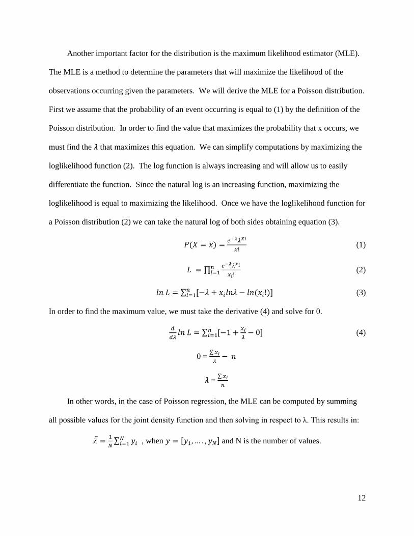
Another important factor for the distribution is the maximum likelihood estimator (MLE).

The MLE is a method to determine the parameters that will maximize the likelihood of the

observations occurring given the parameters. We will derive the MLE for a Poisson distribution.

First we assume that the probability of an event occurring is equal to (1) by the definition of the

Poisson distribution. In order to find the value that maximizes the probability that x occurs, we

must find the 𝜆 that maximizes this equation. We can simplify computations by maximizing the

loglikelihood function (2). The log function is always increasing and will allow us to easily

differentiate the function. Since the natural log is an increasing function, maximizing the

loglikelihood is equal to maximizing the likelihood. Once we have the loglikelihood function for

a Poisson distribution (2) we can take the natural log of both sides obtaining equation (3).

𝑃(𝑋 = 𝑥) =𝑒−𝜆𝜆𝑋𝑖

𝑥! (1)

𝐿 = ∏𝑒−𝜆𝜆𝑥𝑖

𝑥𝑖!

𝑛𝑖=1 (2)

𝑙𝑛 𝐿 = ∑ [−𝜆 + 𝑥𝑖𝑙𝑛𝜆 − 𝑙𝑛(𝑥𝑖!)]𝑛𝑖=1 (3)

In order to find the maximum value, we must take the derivative (4) and solve for 0.

𝑑

𝑑𝜆𝑙𝑛 𝐿 = ∑ [−1 +

𝑥𝑖

𝜆− 0]𝑛

𝑖=1 (4)

0 = ∑ 𝑥𝑖

𝜆− 𝑛

𝜆 = ∑ 𝑥𝑖

𝑛

In other words, in the case of Poisson regression, the MLE can be computed by summing

all possible values for the joint density function and then solving in respect to λ. This results in:

�̅� =1

𝑁∑ 𝑦𝑖

𝑁𝑖=1 , when 𝑦 = [𝑦1, … . , 𝑦𝑁] and N is the number of values.

13

1.4.3 Distribution Application

Before applying the Poisson model to soccer matches, we must confirm that the occurrence

of goals follows a Poisson distribution. The number of goals that a team scores in a match

appears to be approximately distributed. In “Soccer Goal Probabilities Poisson vs Actual

Distribution” data were gathered from five major leagues to equate to a total of 36,996 games

[11]. The results showed that both the home and away team goal distributions are very similar to

the Poisson regression. These two charts show the similarities between the two distributions.

The distribution proves very similar, except for several small discrepancies for the away team.

Figure 1 - Soccer Home Goals Poisson vs Actual [11]

Figure 2 - Soccer Away Goals Poisson vs Actual [11]

14

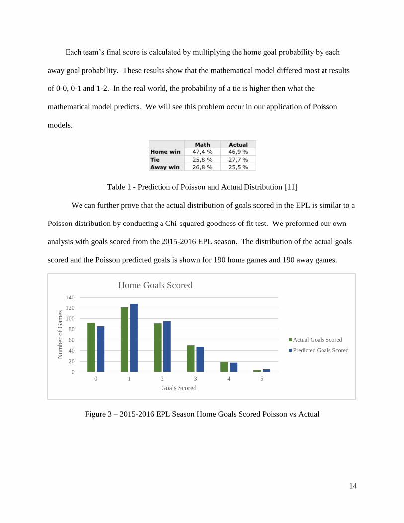
Each team’s final score is calculated by multiplying the home goal probability by each

away goal probability. These results show that the mathematical model differed most at results

of 0-0, 0-1 and 1-2. In the real world, the probability of a tie is higher then what the

mathematical model predicts. We will see this problem occur in our application of Poisson

models.

Table 1 - Prediction of Poisson and Actual Distribution [11]

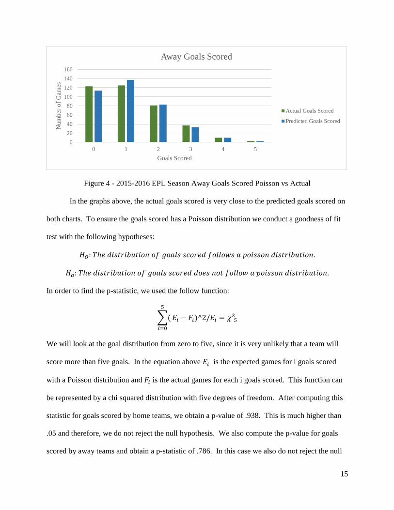
We can further prove that the actual distribution of goals scored in the EPL is similar to a

Poisson distribution by conducting a Chi-squared goodness of fit test. We preformed our own

analysis with goals scored from the 2015-2016 EPL season. The distribution of the actual goals

scored and the Poisson predicted goals is shown for 190 home games and 190 away games.

Figure 3 – 2015-2016 EPL Season Home Goals Scored Poisson vs Actual

0

20

40

60

80

100

120

140

0 1 2 3 4 5

Num

ber

of

Gam

es

Goals Scored

Home Goals Scored

Actual Goals Scored

Predicted Goals Scored

15

Figure 4 - 2015-2016 EPL Season Away Goals Scored Poisson vs Actual

In the graphs above, the actual goals scored is very close to the predicted goals scored on

both charts. To ensure the goals scored has a Poisson distribution we conduct a goodness of fit

test with the following hypotheses:

𝐻𝑂: 𝑇ℎ𝑒 𝑑𝑖𝑠𝑡𝑟𝑖𝑏𝑢𝑡𝑖𝑜𝑛 𝑜𝑓 𝑔𝑜𝑎𝑙𝑠 𝑠𝑐𝑜𝑟𝑒𝑑 𝑓𝑜𝑙𝑙𝑜𝑤𝑠 𝑎 𝑝𝑜𝑖𝑠𝑠𝑜𝑛 𝑑𝑖𝑠𝑡𝑟𝑖𝑏𝑢𝑡𝑖𝑜𝑛.

𝐻𝑎: 𝑇ℎ𝑒 𝑑𝑖𝑠𝑡𝑟𝑖𝑏𝑢𝑡𝑖𝑜𝑛 𝑜𝑓 𝑔𝑜𝑎𝑙𝑠 𝑠𝑐𝑜𝑟𝑒𝑑 𝑑𝑜𝑒𝑠 𝑛𝑜𝑡 𝑓𝑜𝑙𝑙𝑜𝑤 𝑎 𝑝𝑜𝑖𝑠𝑠𝑜𝑛 𝑑𝑖𝑠𝑡𝑟𝑖𝑏𝑢𝑡𝑖𝑜𝑛.

In order to find the p-statistic, we used the follow function:

∑(

5

𝑖=0

𝐸𝑖 − 𝐹𝑖)^2/𝐸𝑖 = 𝜒 52

We will look at the goal distribution from zero to five, since it is very unlikely that a team will

score more than five goals. In the equation above 𝐸𝑖 is the expected games for i goals scored

with a Poisson distribution and 𝐹𝑖 is the actual games for each i goals scored. This function can

be represented by a chi squared distribution with five degrees of freedom. After computing this

statistic for goals scored by home teams, we obtain a p-value of .938. This is much higher than

.05 and therefore, we do not reject the null hypothesis. We also compute the p-value for goals

scored by away teams and obtain a p-statistic of .786. In this case we also do not reject the null

0

20

40

60

80

100

120

140

160

0 1 2 3 4 5

Num

ber

of

Gam

es

Goals Scored

Away Goals Scored

Actual Goals Scored

Predicted Goals Scored

16

hypothesis. We can conclude that home goals scored and away goals scored can be modeled by

a Poisson distribution.

1.5 Variable Analysis

While our model uses the number of goals scored to predict the winner, there are many

factors that help increase the probability that a goal is scored. To score a goal, the player must

shoot the ball. A shot can come from many different situations and passing usually helps to

create opportunities to shoot [12]. Other variables such as crosses, tackles and dribbles can

change the game and create scoring opportunities. Ian McHale and Phil Scarf set out to explain

match outcome by adding additional variables in their paper, “Modelling soccer matches using

bivariate discrete distributions with general dependence structure”. McHale and Scarf do this by

computing the number of shots that each team take takes during a game. In 1997, Pollard and

Reep concluded that a shot on goal is a result of the effectiveness of a team's possession [12].

McHale and Scarf used passes and crosses to model the number of shots, providing insight into a

team’s overall effectiveness while they had possession of the ball.

Further into their analysis, McHale and Scarf looked at the goals, shots, tackles won,

blocks, clearances, crosses, dribbles, passes made, interceptions, fouls, yellow cards and red

cards for the home and away team. Using data from 1048 English Premier League soccer

matches, they found several correlations between shots and goals scored. The most startling

correlation was a negative correlation between home team and away team shots. As the number

of home team shots increased, the number of away team shots decreased while a correlation

between goals scored home and away did not exist [12]. When applying the model parameters to

the model, McHale and Scarf found that several variables were not significant in the data. These

variables included dribbles and yellow and red cards. These values occurred at a slower rate

17

than shots, passes and other variables. While red cards could be a big dictator of a game result,

in many cases a red occurs too late in a game to give the opposing team a one-man advantage for

a significant amount of time. In the end, McHale and Scarf concluded that away team crosses

and passes were more likely to translate to a shot. They also found that fouls called against the

home team had a greater negative impact on the number of home team shots than the same value

for the away team [12].

Statisticians have also considered several other factors to determine their impact on

match outcomes. In 1993, Barnett and Hilditch investigated if artificial fields gave home teams a

greater advantage in the 1980’s and 1990’s [6]. It was also proved that player send offs had a

negative effect on the results of the team with the send-off. Dixon and Robinson investigated the

variations in the rate a home team scores compared to an away team. It was found that these

rates depend on the time that passes in a match and which team is leading the match [13].

Geographical distance to matches was also studied and Clarke and Norman concluded that it was

a significant influencer in match outcomes [14]. The significance could vary based on the

distance and this may be a more critical factor in international soccer matches than soccer

matches within a nation.

SECTION 2

MODEL APPLICATION

There are several steps that we use to construct each model. The first step is to select the

data set to calculate the variables in our model. Next, we select the model that we would like to

use for our prediction. After selecting the model, we must calculate the variables in our model.

Each team will have at least one variable that will be used as input for the model. Finally, we

select the test set of data to evaluate the success of the model. In order to illustrate the steps

18

needed to construct the model, we will predict the results of the first half of the 2016-2017

season using the previous five years of data.

Figure 5- Model Construction Steps

2.1 Data Selection

We have chosen select data from the 2011-2012, 2012-2013, 2013-2014, 2014-2015 and

2015-2016 seasons to tune the models described. Each season’s data consists of 380 games- 38

games for each team, one home and one away for each matchup. Each season’s data has equal

weight in the models. Each season the teams in the English Premier League change, therefore;

out of the current teams in the English Premier League, one team has no past English Premier

League data, three teams have one season of English Premier League data, two teams have two

seasons worth of data, three teams have four seasons worth of data and eleven teams have five

seasons worth of data.

We will begin by looking at the current English Premier League season. There are

several challenges with the 2016-2017 data set. The three team relegation and promotion

structure of the English Premier League prevent the availability of data for teams who are

promoted from the lower levels into the English Premier League. The teams that are promoted

may be in the Premier League for the first time in the last five years or they may have been in the

league in past years. One team in the 2016-2017 Premier League has no previous data from the

English Premier League and five other teams have two or less seasons of data in the English

Premier League. This makes it challenging to calculate statistics for the teams predicted

Data Selection Model Creation CalculationModel

Evaluation with Test Data

19

performance in the league. The only results we can acquire for the teams are numbers from the

lower divisions. These results are against different teams in a league that is less competitive than

the English Premier League. If we were to assign these statistics to the team, we may over-

estimate the team’s strength. We start with the list of 2016-2017 EPL teams shown below.

Team Location

AFC Bournemouth Bournemouth

Arsenal FC London

Burnley FC Burnley

Chelsea FC London

Crystal Palace London

Everton FC Liverpool

Hull City Hull

Leicester City Leicester

Liverpool FC Liverpool

Manchester City Manchester

Manchester United Manchester

Middlesbrough FC Middlesbrough

Southampton FC Southampton

Stoke City Stoke-on-Trent

Sunderland AFC Sunderland

Swansea City Swansea

Tottenham Hotspur London

Watford FC Watford

West Bromwich Albion West Bromwich

West Ham United London

Table 2 - 2016-17 English Premier League Participants

20

We will compensate for the missing data for these teams by using past data from the

teams who were in the league the previous year and were relegated down to the lower division.

We calculate the team statistics for the three teams relegated the previous year. We then assign

the values from the team who was the median statistic (in between the other two teams) to the

team with the missing data.

The relevancy of the data used for model creation is also very important. Many things

about teams can change during a season or in an off-season. Players will leave, players will be

acquired, managers may be fired and hired, and club budgets may rise or fall. These factors can

completely change the success of a team. We want to obtain enough data to improve our model

and the model confidence but we also must insure that the past data is still relevant to the current

model. In this example we will evaluate the models with data from the past five seasons to

ensure we have enough information to represent the teams.

2.2 Model Creation and Calculation

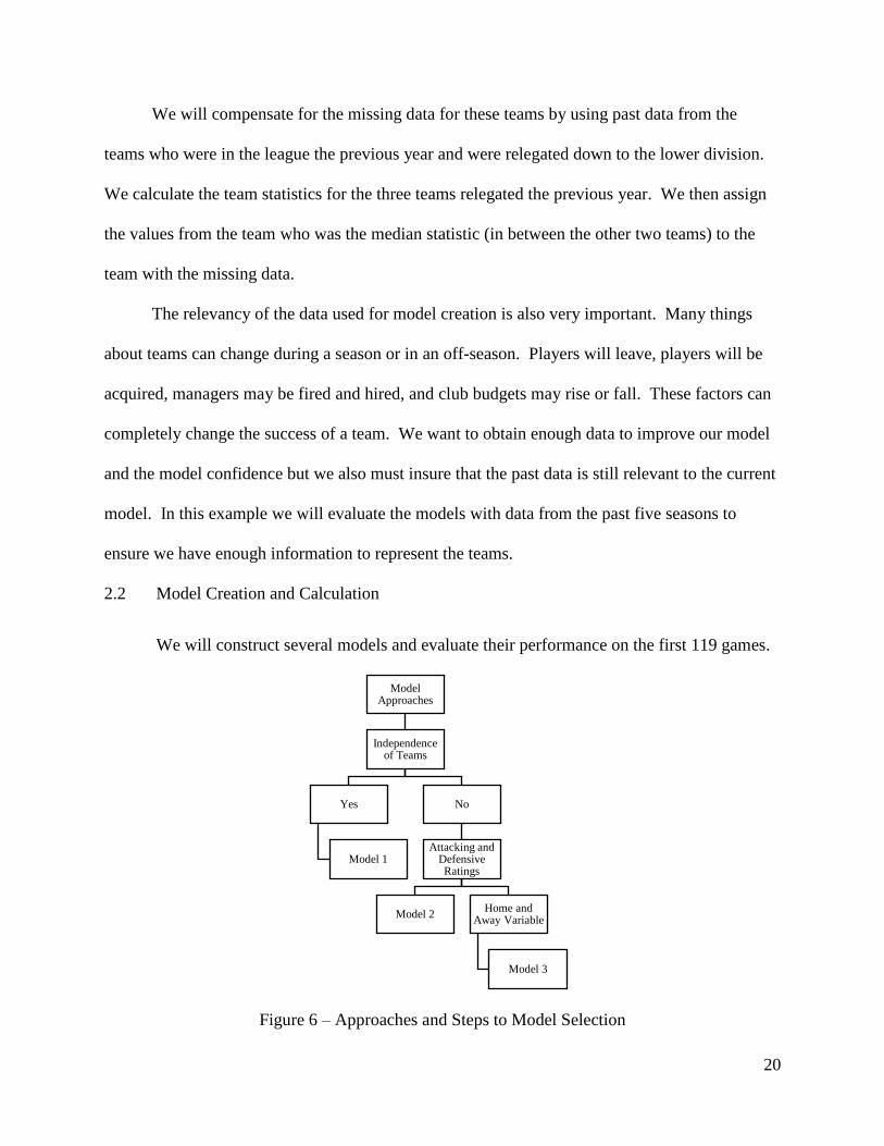
We will construct several models and evaluate their performance on the first 119 games.

Figure 6 – Approaches and Steps to Model Selection

Model Approaches

Independence of Teams

Yes

Model 1

No

Attacking and Defensive Ratings

Model 2Home and

Away Variable

Model 3

21

The models will progress from simplistic to more complex, beginning with a simple model

assuming independence, bivariate and multivariate models and finally a more complex

application. We start with an independent model (Model 1). Next we assume dependence and

add a defensive score (Model 2). Finally we add a final parameter considering if the match was

played at home or away (Model 3).

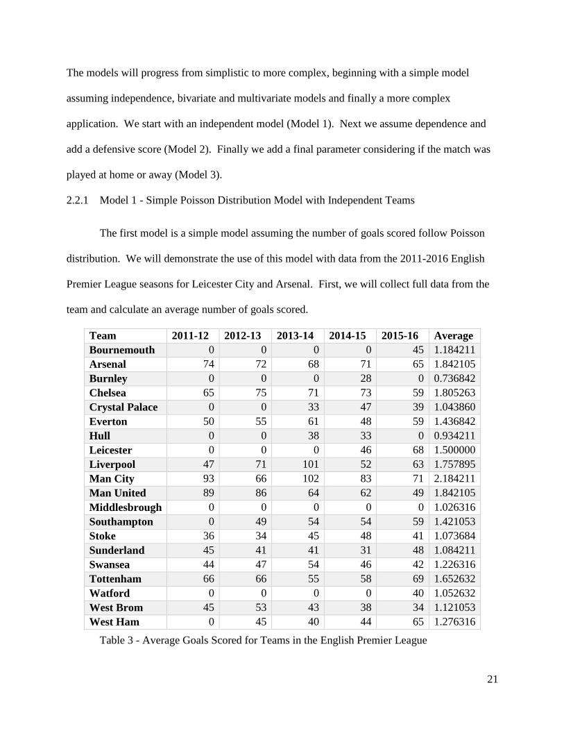
2.2.1 Model 1 - Simple Poisson Distribution Model with Independent Teams

The first model is a simple model assuming the number of goals scored follow Poisson

distribution. We will demonstrate the use of this model with data from the 2011-2016 English

Premier League seasons for Leicester City and Arsenal. First, we will collect full data from the

team and calculate an average number of goals scored.

Team 2011-12 2012-13 2013-14 2014-15 2015-16 Average

Bournemouth 0 0 0 0 45 1.184211

Arsenal 74 72 68 71 65 1.842105

Burnley 0 0 0 28 0 0.736842

Chelsea 65 75 71 73 59 1.805263

Crystal Palace 0 0 33 47 39 1.043860

Everton 50 55 61 48 59 1.436842

Hull 0 0 38 33 0 0.934211

Leicester 0 0 0 46 68 1.500000

Liverpool 47 71 101 52 63 1.757895

Man City 93 66 102 83 71 2.184211

Man United 89 86 64 62 49 1.842105

Middlesbrough 0 0 0 0 0 1.026316

Southampton 0 49 54 54 59 1.421053

Stoke 36 34 45 48 41 1.073684

Sunderland 45 41 41 31 48 1.084211

Swansea 44 47 54 46 42 1.226316

Tottenham 66 66 55 58 69 1.652632

Watford 0 0 0 0 40 1.052632

West Brom 45 53 43 38 34 1.121053

West Ham 0 45 40 44 65 1.276316

Table 3 - Average Goals Scored for Teams in the English Premier League

22

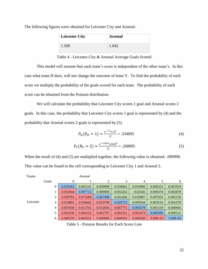
The following figures were obtained for Leicester City and Arsenal:

Leicester City Arsenal

1.500 1.842

Table 4 - Leicester City & Arsenal Average Goals Scored

This model will assume that each team’s score is independent of the other team’s. In this

case what team H does, will not change the outcome of team V. To find the probability of each

score we multiply the probability of the goals scored for each team. The probability of each

score can be obtained from the Poisson distribution.

We will calculate the probability that Leicester City scores 1 goal and Arsenal scores 2

goals. In this case, the probability that Leicester City scores 1 goal is represented by (4) and the

probability that Arsenal scores 2 goals is represented by (5).

𝑃𝐻(𝑅𝐻 = 1) =𝑒−1.51.51

1! = .334695 (4)

𝑃𝑉(𝑅𝑉 = 2) =𝑒−1.8421.8422

2! = .268895 (5)

When the result of (4) and (5) are multiplied together, the following value is obtained- .089998.

This value can be found in the cell corresponding to Leicester City 1 and Arsenal 2.

Teams Arsenal

Goals 0 1 2 3 4 5 6

Leicester

0 0.035362 0.065141 0.059999 0.036841 0.016966 0.006251 0.001919

1 0.053044 0.097712 0.089998 0.055262 0.02545 0.009376 0.002879

2 0.039783 0.073284 0.067498 0.041446 0.019087 0.007032 0.002159

3 0.019891 0.036642 0.033749 0.020723 0.009544 0.003516 0.001079

4 0.007459 0.013741 0.012656 0.007771 0.003579 0.001319 0.000405

5 0.002238 0.004122 0.003797 0.002331 0.001074 0.000396 0.000121

6 0.000559 0.001031 0.000949 0.000583 0.000268 9.89E-05 3.04E-05

Table 5 - Poisson Results for Each Score Line

23

Once the probability of 0, 1, 2, 3, 4, 5 and more goals are obtained for both Arsenal and

Leicester City, we will multiply these probabilities to complete table 5 above. We could carry

these probabilities further out, but the chance of a team scoring more than 8 goals is not likely

and will not produce a significant probability.

Each cell (1-0, 0-1, 0-0) is labeled as a team H win (red), team V win (green) or tie (blue)

and is added to the appropriate match result. The probabilities for an Arsenal win, Leicester City

win and a tie can be summed to obtain the probabilities below:

Arsenal Win 0.455669

Leicester City Win 0.315071

Tie 0.225301

Table 6 - Probability of Arsenal vs. Leicester City Results Model 1

Based on this model, the probability suggests that Arsenal is most likely to win the

match. Earlier this 2016 season, the two teams did face off and the result was a 0-0 tie.

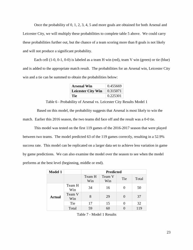
This model was tested on the first 119 games of the 2016-2017 season that were played

between two teams. The model predicted 63 of the 119 games correctly, resulting in a 52.9%

success rate. This model can be replicated on a larger data set to achieve less variation in game

by game predictions. We can also examine the model over the season to see when the model

preforms at the best level (beginning, middle or end).

Model 1 Predicted

Team H

Win

Team V

Win Tie Total

Actual

Team H

Win 34 16 0 50

Team V

Win 8 29 0 37

Tie 17 15 0 32

Total 59 60 0 119

Table 7 - Model 1 Results

24

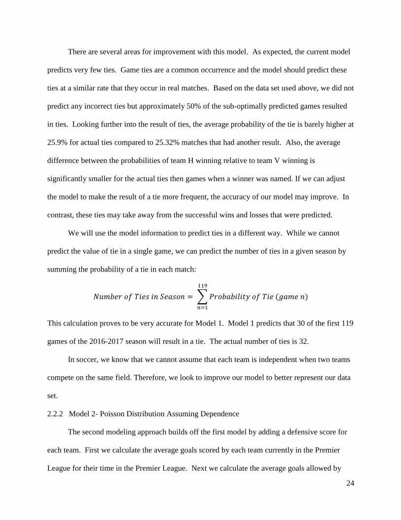
There are several areas for improvement with this model. As expected, the current model

predicts very few ties. Game ties are a common occurrence and the model should predict these

ties at a similar rate that they occur in real matches. Based on the data set used above, we did not

predict any incorrect ties but approximately 50% of the sub-optimally predicted games resulted

in ties. Looking further into the result of ties, the average probability of the tie is barely higher at

25.9% for actual ties compared to 25.32% matches that had another result. Also, the average

difference between the probabilities of team H winning relative to team V winning is

significantly smaller for the actual ties then games when a winner was named. If we can adjust

the model to make the result of a tie more frequent, the accuracy of our model may improve. In

contrast, these ties may take away from the successful wins and losses that were predicted.

We will use the model information to predict ties in a different way. While we cannot

predict the value of tie in a single game, we can predict the number of ties in a given season by

summing the probability of a tie in each match:

𝑁𝑢𝑚𝑏𝑒𝑟 𝑜𝑓 𝑇𝑖𝑒𝑠 𝑖𝑛 𝑆𝑒𝑎𝑠𝑜𝑛 = ∑ 𝑃𝑟𝑜𝑏𝑎𝑏𝑖𝑙𝑖𝑡𝑦 𝑜𝑓 𝑇𝑖𝑒 (𝑔𝑎𝑚𝑒 𝑛)

119

𝑛=1

This calculation proves to be very accurate for Model 1. Model 1 predicts that 30 of the first 119

games of the 2016-2017 season will result in a tie. The actual number of ties is 32.

In soccer, we know that we cannot assume that each team is independent when two teams

compete on the same field. Therefore, we look to improve our model to better represent our data

set.

2.2.2 Model 2- Poisson Distribution Assuming Dependence

The second modeling approach builds off the first model by adding a defensive score for

each team. First we calculate the average goals scored by each team currently in the Premier

League for their time in the Premier League. Next we calculate the average goals allowed by

25

each team in the 2016-2017 English Premier League. The chart for these averages is shown

below. Only one of the teams currently in the Premier League does not have any previous

Premier League data - Middlesborough. For this team we calculate the average number of goals

scored and conceded for the three team’s – Newcastle, Norwich City and Aston Villa - that were

relegated out of the premier league the previous year and assign the median value of the three

relegated teams.

2011-12 2012-13 2013-14 2014-15 2015-16 AVERAGE

Arsenal 49 37 41 36 36 1.047368

Bournemouth 0 0 0 0 67 1.763158

Burnley 0 0 0 53 0 1.394737

Chelsea 46 39 27 32 53 1.036842

Crystal Palace 0 0 48 51 51 1.315789

Everton 40 40 39 50 55 1.178947

Hull 0 0 53 51 0 1.368421

Leicester 0 0 0 55 36 1.197368

Liverpool 40 43 50 48 50 1.215789

Man City 29 34 37 38 41 0.942105

Man United 33 43 43 37 35 1.005263

Middlesbrough 0 0 0 0 0 1.763158

Southampton 0 60 46 33 41 1.184211

Stoke 53 45 52 45 55 1.315789

Sunderland 46 54 60 53 62 1.447368

Swansea 51 51 54 49 52 1.352632

Tottenham 41 46 51 53 35 1.189474

Watford 0 0 0 0 50 1.315789

West Brom 52 57 59 51 48 1.405263

West Ham 0 53 51 47 51 1.328947

Table 8 - Average Goals Conceded for Teams in the English Premier League

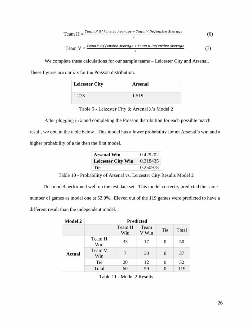
After calculating the offensive and defensive goals allowed for each team, we use a

Poisson distribution to calculate the probability of each result. In this model, our λ for Team H

became the offensive score of Team H plus the defensive score of team V and then divided by

two (6). Our λ for team V became the offensive score of team V plus the defensive score of team

H and then divided by two (7).

26

Team H = 𝑇𝑒𝑎𝑚 𝐻 𝑂𝑓𝑓𝑒𝑛𝑠𝑖𝑣𝑒 𝐴𝑣𝑒𝑟𝑎𝑔𝑒 + 𝑇𝑒𝑎𝑚 𝑉 𝐷𝑒𝑓𝑒𝑛𝑠𝑖𝑣𝑒 𝐴𝑣𝑒𝑟𝑎𝑔𝑒

2 (6)

Team V = 𝑇𝑒𝑎𝑚 𝑉 𝑂𝑓𝑓𝑒𝑛𝑠𝑖𝑣𝑒 𝐴𝑣𝑒𝑟𝑎𝑔𝑒 + 𝑇𝑒𝑎𝑚 𝐻 𝐷𝑒𝑓𝑒𝑛𝑠𝑖𝑣𝑒 𝐴𝑣𝑒𝑟𝑎𝑔𝑒

2 (7)

We complete these calculations for our sample teams – Leicester City and Arsenal.

These figures are our λ’s for the Poisson distribution.


1.273 1.519

Table 9 - Leicester City & Arsenal λ’s Model 2

After plugging in λ and completing the Poisson distribution for each possible match

result, we obtain the table below. This model has a lower probability for an Arsenal’s win and a

higher probability of a tie then the first model.



Tie 0.250978


This model performed well on the test data set. This model correctly predicted the same

number of games as model one at 52.9%. Eleven out of the 119 games were predicted to have a

different result than the independent model.

Model 2 Predicted

Team H

Win

Team

V Win Tie Total

Actual

Team H

Win 33 17 0 50

Team V

Win 7 30 0 37

Tie 20 12 0 32

Total 60 59 0 119


27

This model predicts all the ties incorrectly. Again, this is a major flaw in the model. The

average difference between the probabilities of team H winning relative to team V winning is

smaller for the actual ties then in games when a winner was named. Like model 1, the average

probability that a team ties on true ties is almost equal to the probability of a tie for false ties. If

we sum the tie probabilities for each match in the season, model two predicts 31 ties, preforming

slightly better than model 1.

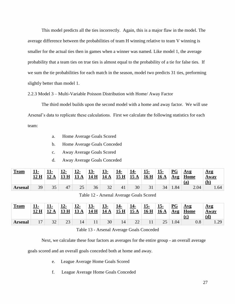
2.2.3 Model 3 – Multi-Variable Poisson Distribution with Home/ Away Factor

The third model builds upon the second model with a home and away factor. We will use

Arsenal’s data to replicate these calculations. First we calculate the following statistics for each

team:

a. Home Average Goals Scored

b. Home Average Goals Conceded

c. Away Average Goals Scored

d. Away Average Goals Conceded

Team 11-

12 H

11-

12 A

12-

13 H

12-

13 A

13-

14 H

13-

14 A

14-

15 H

14-

15 A

15-

16 H

15-

16 A

PG

Avg

Avg

Home

(a)

Avg

Away

(b)

Arsenal 39 35 47 25 36 32 41 30 31 34 1.84 2.04 1.64

Table 12 - Arsenal Average Goals Scored

Team 11-

12 H

11-

12 A

12-

13 H

12-

13 A

13-

14 H

13-

14 A

14-

15 H

14-

15 A

15-

16 H

15-

16 A

PG

Avg

Avg

Home

(c)

Avg

Away

(d)

Arsenal 17 32 23 14 11 30 14 22 11 25 1.04 0.8 1.29

Table 13 - Arsenal Average Goals Conceded

Next, we calculate these four factors as averages for the entire group - an overall average

goals scored and an overall goals conceded both at home and away.

e. League Average Home Goals Scored

f. League Average Home Goals Conceded

28

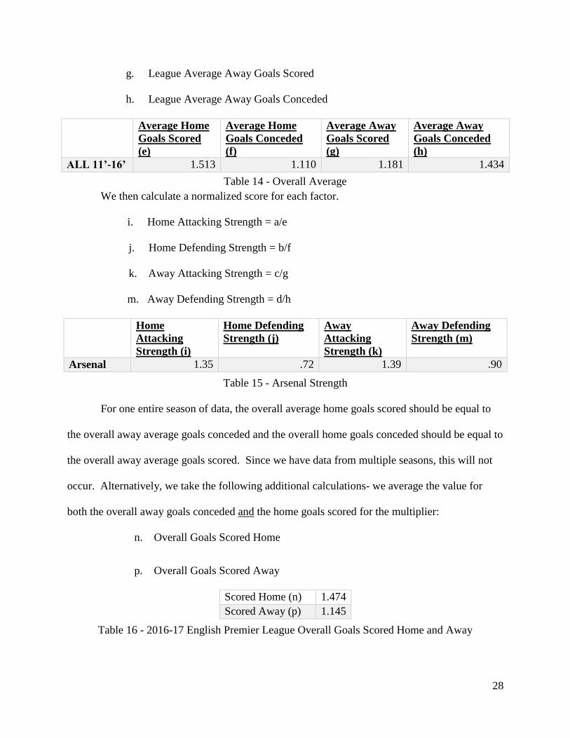
g. League Average Away Goals Scored

h. League Average Away Goals Conceded

Average Home

Goals Scored

(e)

Average Home

Goals Conceded

(f)

Average Away

Goals Scored

(g)

Average Away

Goals Conceded

(h)

ALL 11’-16’ 1.513 1.110 1.181 1.434

Table 14 - Overall Average

We then calculate a normalized score for each factor.

i. Home Attacking Strength = a/e

j. Home Defending Strength = b/f

k. Away Attacking Strength = c/g

m. Away Defending Strength = d/h

Home

Attacking

Strength (i)

Home Defending

Strength (j)

Away

Attacking

Strength (k)

Away Defending

Strength (m)

Arsenal 1.35 .72 1.39 .90

Table 15 - Arsenal Strength

For one entire season of data, the overall average home goals scored should be equal to

the overall away average goals conceded and the overall home goals conceded should be equal to

the overall away average goals scored. Since we have data from multiple seasons, this will not

occur. Alternatively, we take the following additional calculations- we average the value for

both the overall away goals conceded and the home goals scored for the multiplier:

n. Overall Goals Scored Home

p. Overall Goals Scored Away

Scored Home (n) 1.474

Scored Away (p) 1.145

Table 16 - 2016-17 English Premier League Overall Goals Scored Home and Away

29

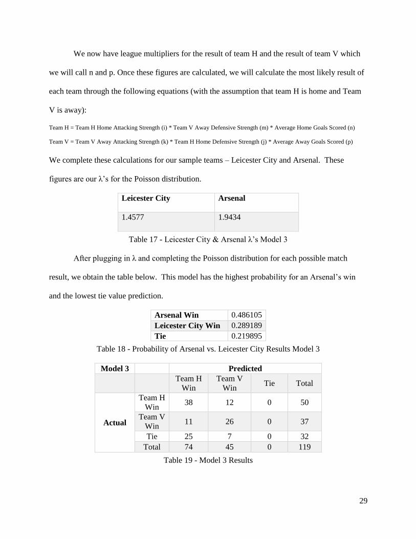
We now have league multipliers for the result of team H and the result of team V which

we will call n and p. Once these figures are calculated, we will calculate the most likely result of

each team through the following equations (with the assumption that team H is home and Team

V is away):

Team H = Team H Home Attacking Strength (i) * Team V Away Defensive Strength (m) * Average Home Goals Scored (n)

Team V = Team V Away Attacking Strength (k) * Team H Home Defensive Strength (j) * Average Away Goals Scored (p)

We complete these calculations for our sample teams – Leicester City and Arsenal. These

figures are our λ’s for the Poisson distribution.


1.4577 1.9434

Table 17 - Leicester City & Arsenal λ’s Model 3

After plugging in λ and completing the Poisson distribution for each possible match

result, we obtain the table below. This model has the highest probability for an Arsenal’s win

and the lowest tie value prediction.



Tie 0.219895


Model 3 Predicted

Team H

Win

Team V

Win Tie Total

Actual

Team H

Win 38 12 0 50

Team V

Win 11 26 0 37

Tie 25 7 0 32

Total 74 45 0 119


30

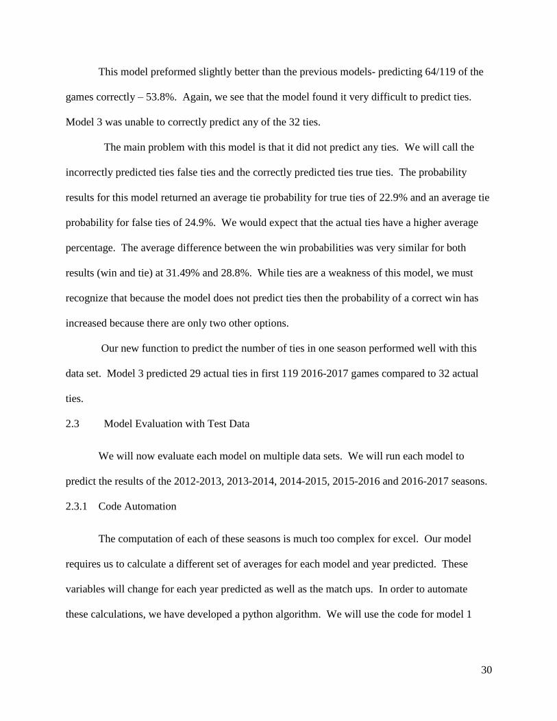
This model preformed slightly better than the previous models- predicting 64/119 of the

games correctly – 53.8%. Again, we see that the model found it very difficult to predict ties.

Model 3 was unable to correctly predict any of the 32 ties.

The main problem with this model is that it did not predict any ties. We will call the

incorrectly predicted ties false ties and the correctly predicted ties true ties. The probability

results for this model returned an average tie probability for true ties of 22.9% and an average tie

probability for false ties of 24.9%. We would expect that the actual ties have a higher average

percentage. The average difference between the win probabilities was very similar for both

results (win and tie) at 31.49% and 28.8%. While ties are a weakness of this model, we must

recognize that because the model does not predict ties then the probability of a correct win has

increased because there are only two other options.

Our new function to predict the number of ties in one season performed well with this

data set. Model 3 predicted 29 actual ties in first 119 2016-2017 games compared to 32 actual

ties.

2.3 Model Evaluation with Test Data

We will now evaluate each model on multiple data sets. We will run each model to

predict the results of the 2012-2013, 2013-2014, 2014-2015, 2015-2016 and 2016-2017 seasons.

2.3.1 Code Automation

The computation of each of these seasons is much too complex for excel. Our model

requires us to calculate a different set of averages for each model and year predicted. These

variables will change for each year predicted as well as the match ups. In order to automate

these calculations, we have developed a python algorithm. We will use the code for model 1

31

with five years of data to predict the 2016-2017 season to demonstrate the structure. Sections of

the full code can be found in the code appendix. The structure of the code is as follows:

1. Import the necessary CSV Files – In order to make our calculations, we must obtain files

that contain data on each seasons match ups, results, betting figures and other variables.

These files were downloaded in a uniform format from Football-Data.co.uk [15]. We

store all past year files in a list [Code 1] and save the current year we are attempting to

predict with only the variables necessary for prediction (match-up, result (if available)

and betting odds). [Code 2] Next we set of number of games variable equal to the number

of games in the prediction file plus one value for iterating through the lists. [Code 3]

2. Set List Values for All Necessary Variables – Now we must create a list for each file we

want to save in our calculations. We save the home team, away team, actual home team

goals scored, actual away team goals scored, match probabilities: home team win, away

team win and tie, actual result of the match, predicted match results and the accuracy of

the prediction. [Code 4]

3. Calculate Average Values for Each Team - We must calculate the average value for each

team in the prediction season. To do this we use a stored list of teams in the league for

the 2016-2017 season [Code 5] and iterate through two loops to sum the number of goals

for each season that the current season teams were in the English Premier League [Code

6]. Since all teams were not in the English Premier League for all five years, we create

another list specifying the number of previous seasons in the past five years that each

team was in the English Premier League. We sum the value of each team’s seasonal data

and divide the total goals by the number of years each team was in the English Premier

League. [Code 7] In our example there is one team missing data. For this team we add a

32

one in our list of past data (to allow the calculation). Once the calculation has occurred,

we replace the list value of the team with the average computed from the middle team

that was relegated the previous year. We save the final average in a new csv file.

4. Write File to Store Information – We create a file to store all game past game information

and our final information. This file includes the home team, away team and the goals

scored for each team. [Code 8]

5. Calculate the Predicted Result of Each Match – Now that we have our average values, we

predict the result of each match by finding the highest probable result. We locate the

home team and away team from the place in our previous file. We calculate this result

and save it to a new list. After this calculation is complete, we move onto the next match.

[Code 9]

6. Determine if Prediction is Correct – Once we have predicted the result of each match, we

determine if the match prediction is correct by checking to see if the place marker list

value is equivalent in predicted result and actual result. [Code 10]

7. Final Results – From these calculations we determine the number of successful

predictions for the season, the number of correct predictions excluding ties and the

expected value of ties [Code 11].

8. Add Results to File – We now write all results to our prior file and save for reference.

2.3.2 Expanded Data Analysis

We will now test our models on the first 283 games of the 2016-2017 English Premier

League Season and the full 380 games of the 2012-2013, 2013-2014, 2014-2015 and 2016-2017

seasons. We compute two averages for each model, an average that includes all full seasons of

data and an average that includes the predictions for the current season that has not yet finished.

33

We will refer to the full seasons of data throughout our analysis since we do not know the full

details of the 2016-2017 season.

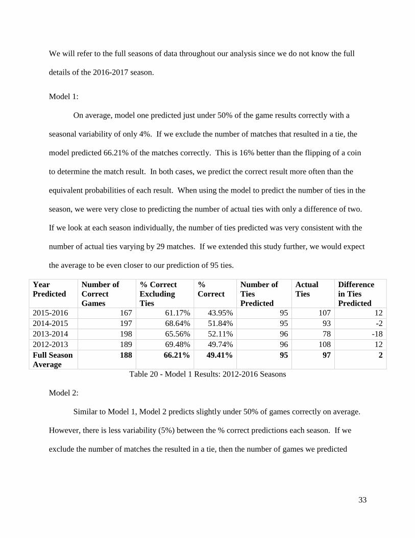
Model 1:

On average, model one predicted just under 50% of the game results correctly with a

seasonal variability of only 4%. If we exclude the number of matches that resulted in a tie, the

model predicted 66.21% of the matches correctly. This is 16% better than the flipping of a coin

to determine the match result. In both cases, we predict the correct result more often than the

equivalent probabilities of each result. When using the model to predict the number of ties in the

season, we were very close to predicting the number of actual ties with only a difference of two.

If we look at each season individually, the number of ties predicted was very consistent with the

number of actual ties varying by 29 matches. If we extended this study further, we would expect

the average to be even closer to our prediction of 95 ties.

Year

Predicted

Number of

Correct

Games

% Correct

Excluding

Ties

%

Correct

Number of

Ties

Predicted

Actual

Ties

Difference

in Ties

Predicted

2015-2016 167 61.17% 43.95% 95 107 12

2014-2015 197 68.64% 51.84% 95 93 -2

2013-2014 198 65.56% 52.11% 96 78 -18

2012-2013 189 69.48% 49.74% 96 108 12

Full Season

Average

188 66.21% 49.41% 95 97 2

Table 20 - Model 1 Results: 2012-2016 Seasons

Model 2:

Similar to Model 1, Model 2 predicts slightly under 50% of games correctly on average.

However, there is less variability (5%) between the % correct predictions each season. If we

exclude the number of matches the resulted in a tie, then the number of games we predicted

34

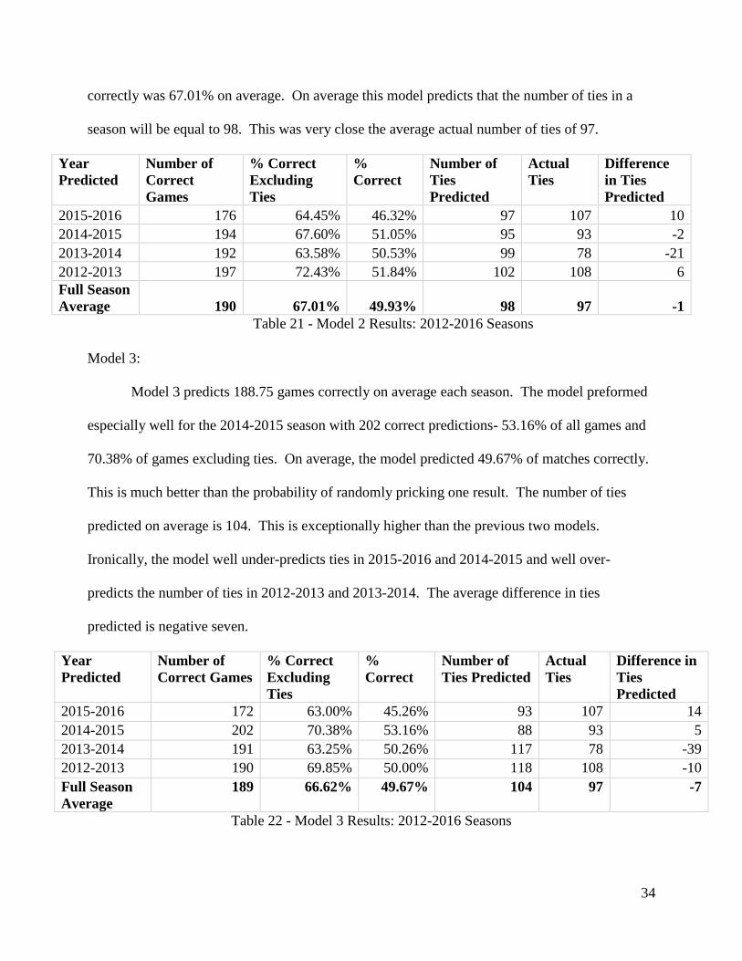
correctly was 67.01% on average. On average this model predicts that the number of ties in a

season will be equal to 98. This was very close the average actual number of ties of 97.

Year

Predicted

Number of

Correct

Games

% Correct

Excluding

Ties

%

Correct

Number of

Ties

Predicted

Actual

Ties

Difference

in Ties

Predicted

2015-2016 176 64.45% 46.32% 97 107 10

2014-2015 194 67.60% 51.05% 95 93 -2

2013-2014 192 63.58% 50.53% 99 78 -21

2012-2013 197 72.43% 51.84% 102 108 6

Full Season

Average 190 67.01% 49.93% 98 97 -1


Model 3:

Model 3 predicts 188.75 games correctly on average each season. The model preformed

especially well for the 2014-2015 season with 202 correct predictions- 53.16% of all games and

70.38% of games excluding ties. On average, the model predicted 49.67% of matches correctly.

This is much better than the probability of randomly pricking one result. The number of ties

predicted on average is 104. This is exceptionally higher than the previous two models.

Ironically, the model well under-predicts ties in 2015-2016 and 2014-2015 and well over-

predicts the number of ties in 2012-2013 and 2013-2014. The average difference in ties

predicted is negative seven.

Year

Predicted

Number of

Correct Games

% Correct

Excluding

Ties

%

Correct

Number of

Ties Predicted

Actual

Ties

Difference in

Ties

Predicted

2015-2016 172 63.00% 45.26% 93 107 14

2014-2015 202 70.38% 53.16% 88 93 5

2013-2014 191 63.25% 50.26% 117 78 -39

2012-2013 190 69.85% 50.00% 118 108 -10

Full Season

Average

189 66.62% 49.67% 104 97 -7


35

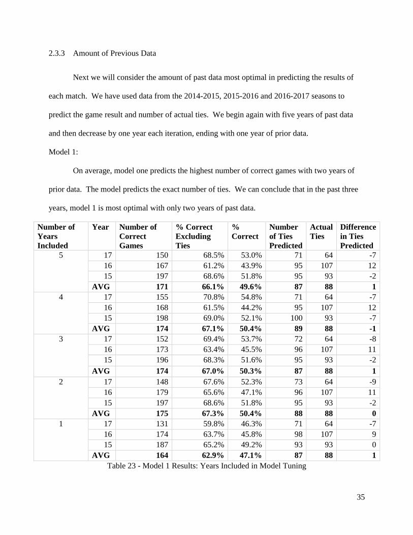
2.3.3 Amount of Previous Data

Next we will consider the amount of past data most optimal in predicting the results of

each match. We have used data from the 2014-2015, 2015-2016 and 2016-2017 seasons to

predict the game result and number of actual ties. We begin again with five years of past data

and then decrease by one year each iteration, ending with one year of prior data.

Model 1:

On average, model one predicts the highest number of correct games with two years of

prior data. The model predicts the exact number of ties. We can conclude that in the past three

years, model 1 is most optimal with only two years of past data.

Number of

Years

Included

Year Number of

Correct

Games

% Correct

Excluding

Ties

%

Correct

Number

of Ties

Predicted

Actual

Ties

Difference

in Ties

Predicted

5 17 150 68.5% 53.0% 71 64 -7

16 167 61.2% 43.9% 95 107 12

15 197 68.6% 51.8% 95 93 -2

AVG 171 66.1% 49.6% 87 88 1

4 17 155 70.8% 54.8% 71 64 -7

16 168 61.5% 44.2% 95 107 12

15 198 69.0% 52.1% 100 93 -7

AVG 174 67.1% 50.4% 89 88 -1

3 17 152 69.4% 53.7% 72 64 -8

16 173 63.4% 45.5% 96 107 11

15 196 68.3% 51.6% 95 93 -2

AVG 174 67.0% 50.3% 87 88 1

2 17 148 67.6% 52.3% 73 64 -9

16 179 65.6% 47.1% 96 107 11

15 197 68.6% 51.8% 95 93 -2

AVG 175 67.3% 50.4% 88 88 0

1 17 131 59.8% 46.3% 71 64 -7

16 174 63.7% 45.8% 98 107 9

15 187 65.2% 49.2% 93 93 0

AVG 164 62.9% 47.1% 87 88 1

Table 23 - Model 1 Results: Years Included in Model Tuning

36

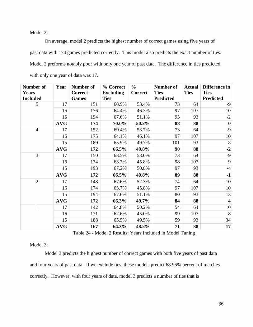
Model 2:

On average, model 2 predicts the highest number of correct games using five years of

past data with 174 games predicted correctly. This model also predicts the exact number of ties.

Model 2 preforms notably poor with only one year of past data. The difference in ties predicted

with only one year of data was 17.

Number of

Years

Included

Year Number of

Correct

Games

% Correct

Excluding

Ties

%

Correct

Number of

Ties

Predicted

Actual

Ties

Difference in

Ties

Predicted

5 17 151 68.9% 53.4% 73 64 -9

16 176 64.4% 46.3% 97 107 10

15 194 67.6% 51.1% 95 93 -2

AVG 174 70.0% 50.2% 88 88 0

4 17 152 69.4% 53.7% 73 64 -9

16 175 64.1% 46.1% 97 107 10

15 189 65.9% 49.7% 101 93 -8

AVG 172 66.5% 49.8% 90 88 -2

3 17 150 68.5% 53.0% 73 64 -9

16 174 63.7% 45.8% 98 107 9

15 193 67.2% 50.8% 97 93 -4

AVG 172 66.5% 49.8% 89 88 -1

2 17 148 67.6% 52.3% 74 64 -10

16 174 63.7% 45.8% 97 107 10

15 194 67.6% 51.1% 80 93 13

AVG 172 66.3% 49.7% 84 88 4

1 17 142 64.8% 50.2% 54 64 10

16 171 62.6% 45.0% 99 107 8

15 188 65.5% 49.5% 59 93 34

AVG 167 64.3% 48.2% 71 88 17


Model 3:

Model 3 predicts the highest number of correct games with both five years of past data

and four years of past data. If we exclude ties, these models predict 68.96% percent of matches

correctly. However, with four years of data, model 3 predicts a number of ties that is

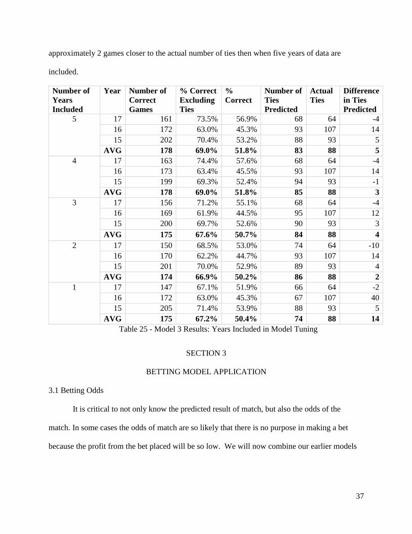
37

approximately 2 games closer to the actual number of ties then when five years of data are

included.

Number of

Years

Included

Year Number of

Correct

Games

% Correct

Excluding

Ties

%

Correct

Number of

Ties

Predicted

Actual

Ties

Difference

in Ties

Predicted

5 17 161 73.5% 56.9% 68 64 -4

16 172 63.0% 45.3% 93 107 14

15 202 70.4% 53.2% 88 93 5

AVG 178 69.0% 51.8% 83 88 5

4 17 163 74.4% 57.6% 68 64 -4

16 173 63.4% 45.5% 93 107 14

15 199 69.3% 52.4% 94 93 -1

AVG 178 69.0% 51.8% 85 88 3

3 17 156 71.2% 55.1% 68 64 -4

16 169 61.9% 44.5% 95 107 12

15 200 69.7% 52.6% 90 93 3

AVG 175 67.6% 50.7% 84 88 4

2 17 150 68.5% 53.0% 74 64 -10

16 170 62.2% 44.7% 93 107 14

15 201 70.0% 52.9% 89 93 4

AVG 174 66.9% 50.2% 86 88 2

1 17 147 67.1% 51.9% 66 64 -2

16 172 63.0% 45.3% 67 107 40

15 205 71.4% 53.9% 88 93 5

AVG 175 67.2% 50.4% 74 88 14


SECTION 3

BETTING MODEL APPLICATION

3.1 Betting Odds

It is critical to not only know the predicted result of match, but also the odds of the

match. In some cases the odds of match are so likely that there is no purpose in making a bet

because the profit from the bet placed will be so low. We will now combine our earlier models

38

with the betting odds for each match to determine if we should place a bet on the match, and if

we were to place a bet on the match, how much we could win.

3.1.1 Types of Odds

In order to apply a profit model to our predictions, we must first understand the betting

odds released by bookies.

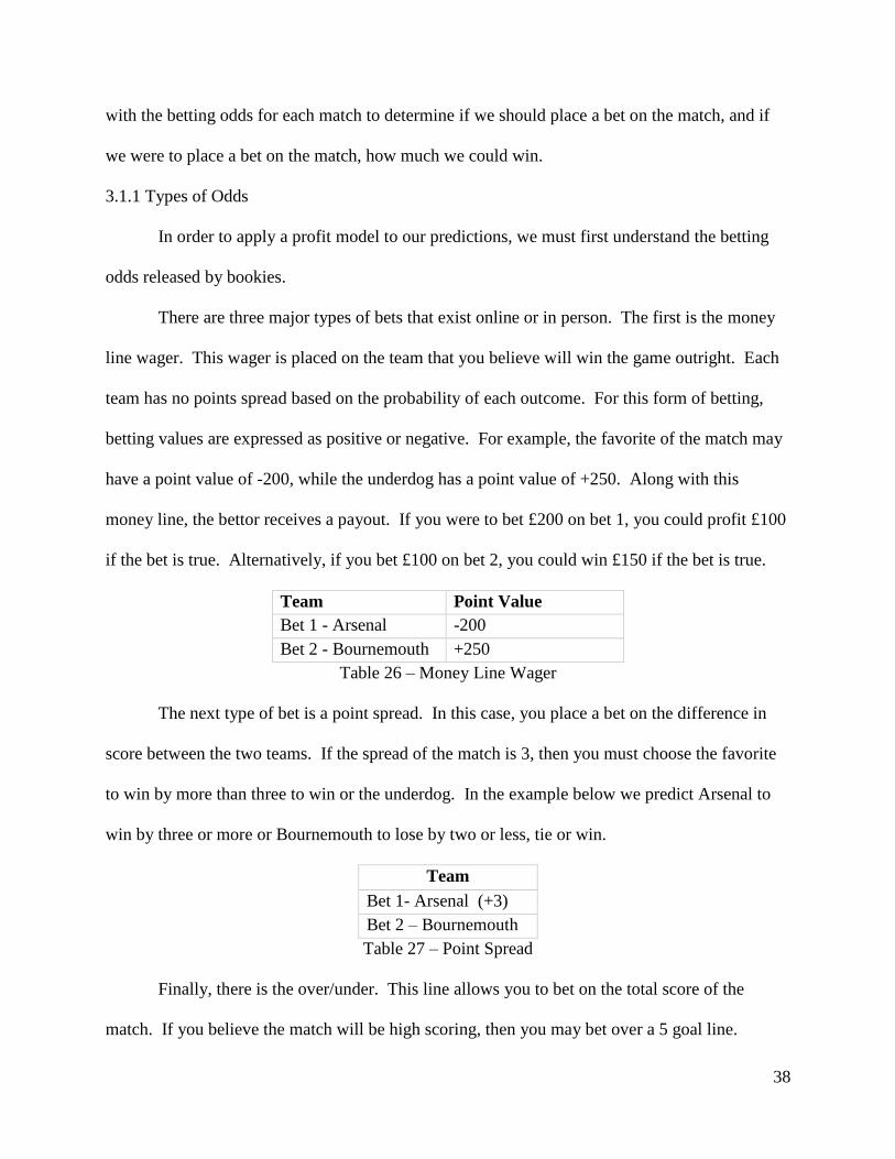
There are three major types of bets that exist online or in person. The first is the money

line wager. This wager is placed on the team that you believe will win the game outright. Each

team has no points spread based on the probability of each outcome. For this form of betting,

betting values are expressed as positive or negative. For example, the favorite of the match may

have a point value of -200, while the underdog has a point value of +250. Along with this

money line, the bettor receives a payout. If you were to bet £200 on bet 1, you could profit £100

if the bet is true. Alternatively, if you bet £100 on bet 2, you could win £150 if the bet is true.

Team Point Value

Bet 1 - Arsenal -200

Bet 2 - Bournemouth +250

Table 26 – Money Line Wager

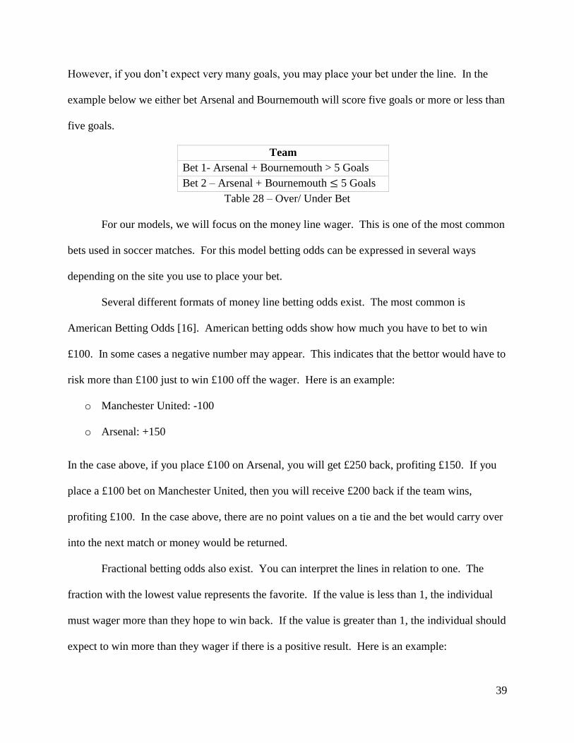
The next type of bet is a point spread. In this case, you place a bet on the difference in

score between the two teams. If the spread of the match is 3, then you must choose the favorite

to win by more than three to win or the underdog. In the example below we predict Arsenal to

win by three or more or Bournemouth to lose by two or less, tie or win.

Team

Bet 1- Arsenal (+3)

Bet 2 – Bournemouth

Table 27 – Point Spread

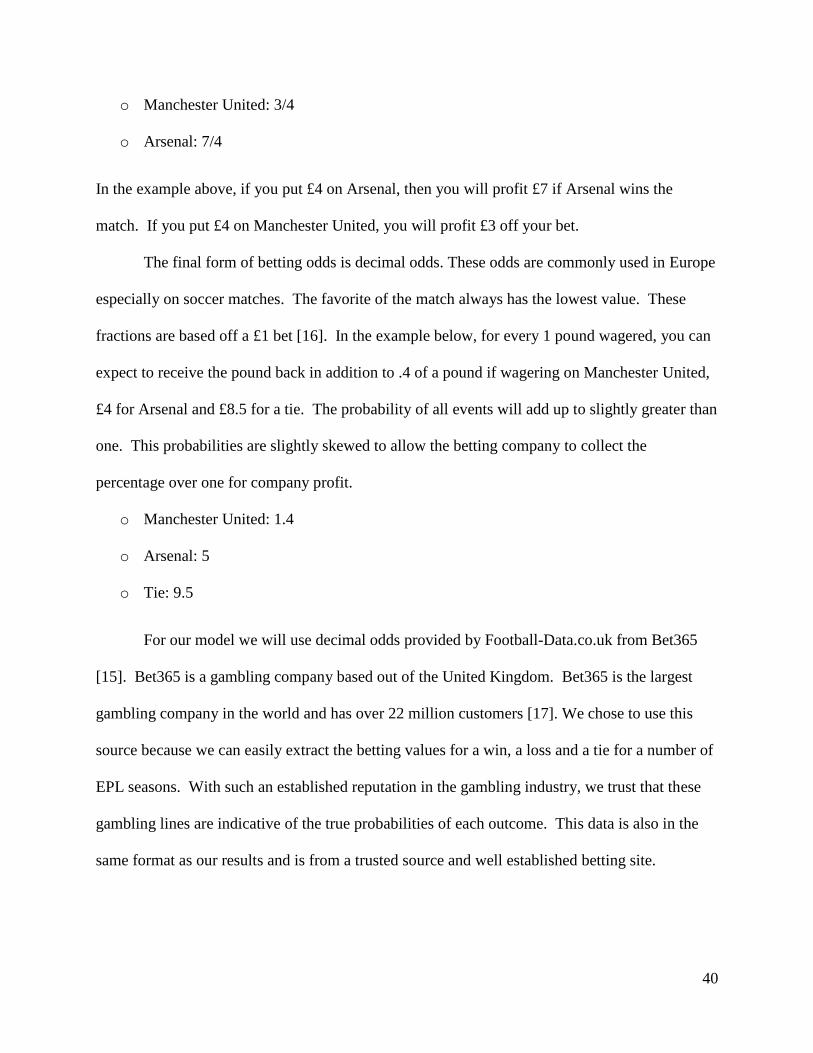
Finally, there is the over/under. This line allows you to bet on the total score of the

match. If you believe the match will be high scoring, then you may bet over a 5 goal line.

39

However, if you don’t expect very many goals, you may place your bet under the line. In the

example below we either bet Arsenal and Bournemouth will score five goals or more or less than

five goals.

Team

Bet 1- Arsenal + Bournemouth > 5 Goals

Bet 2 – Arsenal + Bournemouth ≤ 5 Goals

Table 28 – Over/ Under Bet

For our models, we will focus on the money line wager. This is one of the most common

bets used in soccer matches. For this model betting odds can be expressed in several ways

depending on the site you use to place your bet.

Several different formats of money line betting odds exist. The most common is

American Betting Odds [16]. American betting odds show how much you have to bet to win

£100. In some cases a negative number may appear. This indicates that the bettor would have to

risk more than £100 just to win £100 off the wager. Here is an example:

o Manchester United: -100

o Arsenal: +150

In the case above, if you place £100 on Arsenal, you will get £250 back, profiting £150. If you

place a £100 bet on Manchester United, then you will receive £200 back if the team wins,

profiting £100. In the case above, there are no point values on a tie and the bet would carry over

into the next match or money would be returned.

Fractional betting odds also exist. You can interpret the lines in relation to one. The

fraction with the lowest value represents the favorite. If the value is less than 1, the individual

must wager more than they hope to win back. If the value is greater than 1, the individual should

expect to win more than they wager if there is a positive result. Here is an example:

40

o Manchester United: 3/4

o Arsenal: 7/4

In the example above, if you put £4 on Arsenal, then you will profit £7 if Arsenal wins the

match. If you put £4 on Manchester United, you will profit £3 off your bet.

The final form of betting odds is decimal odds. These odds are commonly used in Europe

especially on soccer matches. The favorite of the match always has the lowest value. These

fractions are based off a £1 bet [16]. In the example below, for every 1 pound wagered, you can

expect to receive the pound back in addition to .4 of a pound if wagering on Manchester United,

£4 for Arsenal and £8.5 for a tie. The probability of all events will add up to slightly greater than

one. This probabilities are slightly skewed to allow the betting company to collect the

percentage over one for company profit.

o Manchester United: 1.4

o Arsenal: 5

o Tie: 9.5

For our model we will use decimal odds provided by Football-Data.co.uk from Bet365

[15]. Bet365 is a gambling company based out of the United Kingdom. Bet365 is the largest

gambling company in the world and has over 22 million customers [17]. We chose to use this

source because we can easily extract the betting values for a win, a loss and a tie for a number of

EPL seasons. With such an established reputation in the gambling industry, we trust that these

gambling lines are indicative of the true probabilities of each outcome. This data is also in the

same format as our results and is from a trusted source and well established betting site.

41

The probability value of each result can be calculated based on the decimal odds placed

on the match. If the decimal odds of a match are: Manchester United – 1.4, Arsenal – 5 and Tie

– 9.5, then we can divide 1 by each value to get the expected probability of each event. This

results in calculations of a 71.4% chance Manchester United will win, a 20% probability Arsenal

will win and 10.5% that the match will result in a tie. These probabilities add up to slightly over

1 at 1.02. This additional two percent goes back to the company that allows users to make the

bet.

3.2 Expected Profit Betting Model

Now that each model gives us the expected probability of each event, we can determine if

we should make a bet based on the probability of each match outcome and the betting odds

provided for each match.

3.2.1 Expected Profit

In order to determine if a bet is worth making, we must determine the expected profit

each bet in a match. The expected profit of a £1 bet for a match x can be calculated for each

prediction:

o Team A Win –

𝐸(𝑥) = (𝐷𝑒𝑐𝑖𝑚𝑎𝑙 𝑂𝑑𝑑𝑠 𝑇𝑒𝑎𝑚 𝐴 − 1) ∗ 𝑃(𝑇𝑒𝑎𝑚 𝐴 𝑊𝑖𝑛) − 1 ∗ 𝑃(𝑇𝑒𝑎𝑚 𝐴 𝐿𝑜𝑠𝑒) − 1 ∗ 𝑃(𝑇𝑖𝑒)

o Team B Win -

𝐸(𝑥) = − 1 ∗ 𝑃(𝑇𝑒𝑎𝑚 𝐴 𝑊𝑖𝑛) + ( 𝐷𝑒𝑐𝑖𝑚𝑎𝑙 𝑂𝑑𝑑𝑠 𝑇𝑒𝑎𝑚 𝐵 − 1) ∗ 𝑃(𝑇𝑒𝑎𝑚 𝐴 𝐿𝑜𝑠𝑒) − 1 ∗ 𝑃(𝑇𝑖𝑒)

o Tie-

𝐸(𝑥) = − 1 ∗ 𝑃(𝑇𝑒𝑎𝑚 𝐴 𝑊𝑖𝑛) − 1 ∗ 𝑃(𝑇𝑒𝑎𝑚 𝐴 𝐿𝑜𝑠𝑒) + (𝐷𝑒𝑐𝑖𝑚𝑎𝑙 𝑂𝑑𝑑𝑠 𝑇𝑖𝑒 − 1) ∗ 𝑃(𝑇𝑖𝑒)

We will extend this equation to the previous example above. If the decimal odds of a match are:

Manchester United – 1.4, Arsenal – 5 and Tie – 9.5 and the probability of Manchester United

winning is .46, the probability of Arsenal winning is .29 and the probability of a tie is .25, then

the appropriate formula for expected profit would be:

42

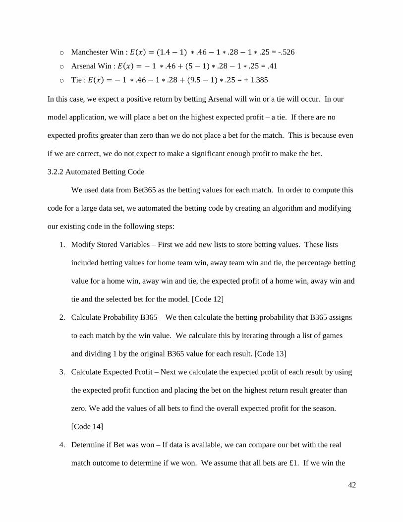
o Manchester Win : 𝐸(𝑥) = (1.4 − 1) ∗ .46 − 1 ∗ .28 − 1 ∗ .25 = -.526

o Arsenal Win : 𝐸(𝑥) = − 1 ∗ .46 + (5 − 1) ∗ .28 − 1 ∗ .25 = .41

o Tie : 𝐸(𝑥) = − 1 ∗ .46 − 1 ∗ .28 + (9.5 − 1) ∗ .25 = + 1.385

In this case, we expect a positive return by betting Arsenal will win or a tie will occur. In our

model application, we will place a bet on the highest expected profit – a tie. If there are no

expected profits greater than zero than we do not place a bet for the match. This is because even

if we are correct, we do not expect to make a significant enough profit to make the bet.

3.2.2 Automated Betting Code

We used data from Bet365 as the betting values for each match. In order to compute this

code for a large data set, we automated the betting code by creating an algorithm and modifying

our existing code in the following steps:

1. Modify Stored Variables – First we add new lists to store betting values. These lists

included betting values for home team win, away team win and tie, the percentage betting

value for a home win, away win and tie, the expected profit of a home win, away win and

tie and the selected bet for the model. [Code 12]

2. Calculate Probability B365 – We then calculate the betting probability that B365 assigns

to each match by the win value. We calculate this by iterating through a list of games

and dividing 1 by the original B365 value for each result. [Code 13]

3. Calculate Expected Profit – Next we calculate the expected profit of each result by using

the expected profit function and placing the bet on the highest return result greater than

zero. We add the values of all bets to find the overall expected profit for the season.

[Code 14]

4. Determine if Bet was won – If data is available, we can compare our bet with the real

match outcome to determine if we won. We assume that all bets are £1. If we win the

43

bet then we add the B365 value assigned to our result and subtract £1 to get the overall

profit. If we lose the bet then we subtract £1 from our overall profit. [code 14]

3.2.3 Betting Results

We used our automated code to calculate the actual value and expected value won for all

three models for the 2012-2013, 2013-2014, 2014-2015 and 2015-2016 seasons and part of the

2016-2017 season. The results are shown below. We chose not to include the 2016-2017 season

in the average because it does not contain a full season.

Model Year Predicted Actual Value Won Expected Value Won

Model

1

2015-2016 £ 21.74 £ 188.10

2014-2015 -£ 25.87 £ 197.68

2013-2014 -£ 22.27 £ 270.21

2012-2013 -£ 58.95 £ 234.70

Full Season Average -£ 21.34 £ 222.67

Model

2

2015-2016 £ 29.60 £ 206.26

2014-2015 -£ 2.87 £ 220.56

2013-2014 -£ 10.52 £ 303.59

2012-2013 -£ 60.02 £ 225.61


Model

3

2015-2016 £ 4.78 £ 94.20

2014-2015 £ 6.71 £ 86.33

2013-2014 -£ 34.85 £ 256.06

2012-2013 -£ 7.76 £ 209.11


Table 29 – Expected Profit Model Comparison 2012-2016 Seasons

All models actually lost money on average. Model 3 lost the least amount of money on

average at -£7.78. However, there was one season where all models were profitable – 2015-

2016. In this season there were a large number of upsets and Leicester City, a team with only

one prior year of EPL experience, won the championship. The actual results are different than

the expected value for each model. Model 2 has both the highest expected value won in a single

year and the highest average expected value won. The expected value won is much higher than

44

the actual value won. In our model we do not place a bet in any case which all expected values

are less than zero. This rarely occurs and we are placing bets in almost every game. In the

future, we can improve our model by setting a higher mark such as .5 or .75 to place our bets or

we can consider a condition where we place multiple bets with a positive expected value.

We also replicated this calculation to determine if the number of years included to

calculate the averages for our model influenced the actual value won and the expected value

won.

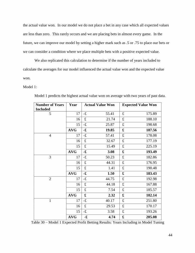
Model 1:

Model 1 predicts the highest actual value won on average with two years of past data.

Number of Years

Included

Year Actual Value Won Expected Value Won

5 17 -£ 55.41 £ 175.89

16 £ 21.74 £ 188.10

15 -£ 25.87 £ 198.68

AVG -£ 19.85 £ 187.56

4 17 -£ 57.41 £ 178.08

16 £ 32.67 £ 177.19

15 £ 15.49 £ 225.19

AVG -£ 3.08 £ 193.49

3 17 -£ 50.23 £ 182.86

16 £ 44.31 £ 176.95

15 £ 1.41 £ 190.48

AVG -£ 1.50 £ 183.43

2 17 -£ 44.75 £ 192.98

16 £ 44.18 £ 167.88

15 £ 7.54 £ 185.57

AVG £ 2.32 £ 182.14

1 17 -£ 40.17 £ 251.80

16 £ 29.53 £ 170.17

15 -£ 3.58 £ 193.26

AVG -£ 4.74 £ 205.08

Table 30 – Model 1 Expected Profit Betting Results: Years Including in Model Tuning

45

The highest actual value won with two years of past data is £2.32 and its corresponding

expected value won is £182.14. However, the highest expected value won occurs with one year

of past data at £205.08. Based on the actual value won, we choose two years of past data to

include as our betting model predictor for model 1.

Model 2:

In model 2, the highest actual value won occurs with five years of data at £2.19. The

year with the highest expected value won is only one year of past data. We conclude that it is

most optimal to use five past years of data in the betting model for model 2.

Number of Years

Included Year Actual Value Won Expected Value Won

5

17 -£ 20.15 £ 81.49

16 £ 29.60 £ 206.26

15 -£ 2.87 £ 220.56

AVG £ 2.19 £ 169.44

4

17 -£ 41.74 £ 219.12

16 £ 28.01 £ 201.39

15 £ 0.25 £ 234.41

AVG -£ 4.49 £ 218.31

3

17 -£ 51.24 £ 221.49

16 £ 28.63 £ 195.88

15 £ 5.86 £ 231.43

AVG -£ 5.58 £ 216.27

2

17 -£ 63.75 £ 228.30

16 £ 29.68 £ 193.92

15 -£ 11.22 £ 238.43

AVG -£ 15.10 £ 220.22

1

17 -£ 32.94 £ 256.07

16 £ 10.73 £ 202.48

15 £ 14.38 £ 245.22

AVG -£ 12.20 £ 234.59

Table 31 – Model 2 Expected Profit Betting Results: Years Included in Model Tuning

46

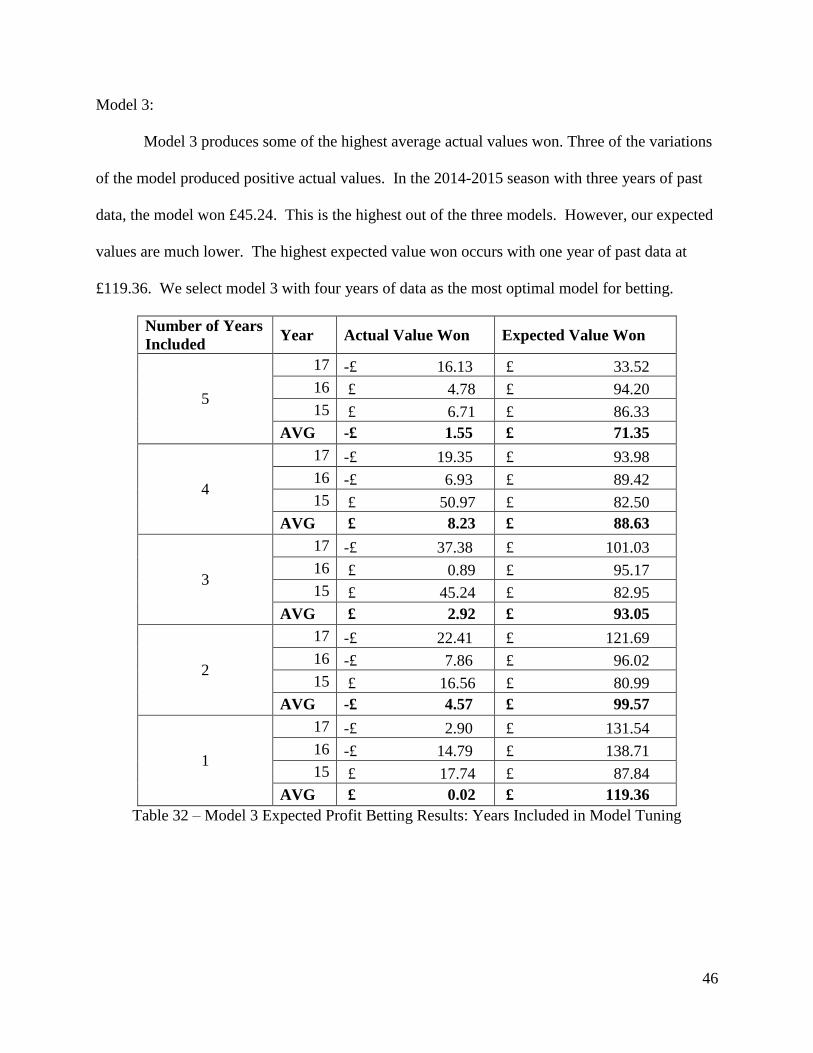
Model 3:

Model 3 produces some of the highest average actual values won. Three of the variations

of the model produced positive actual values. In the 2014-2015 season with three years of past

data, the model won £45.24. This is the highest out of the three models. However, our expected

values are much lower. The highest expected value won occurs with one year of past data at

£119.36. We select model 3 with four years of data as the most optimal model for betting.

Number of Years

Included Year Actual Value Won Expected Value Won

5

17 -£ 16.13 £ 33.52

16 £ 4.78 £ 94.20

15 £ 6.71 £ 86.33

AVG -£ 1.55 £ 71.35

4

17 -£ 19.35 £ 93.98

16 -£ 6.93 £ 89.42

15 £ 50.97 £ 82.50

AVG £ 8.23 £ 88.63

3

17 -£ 37.38 £ 101.03

16 £ 0.89 £ 95.17

15 £ 45.24 £ 82.95

AVG £ 2.92 £ 93.05

2

17 -£ 22.41 £ 121.69

16 -£ 7.86 £ 96.02

15 £ 16.56 £ 80.99

AVG -£ 4.57 £ 99.57

1

17 -£ 2.90 £ 131.54

16 -£ 14.79 £ 138.71

15 £ 17.74 £ 87.84

AVG £ 0.02 £ 119.36

Table 32 – Model 3 Expected Profit Betting Results: Years Included in Model Tuning

47

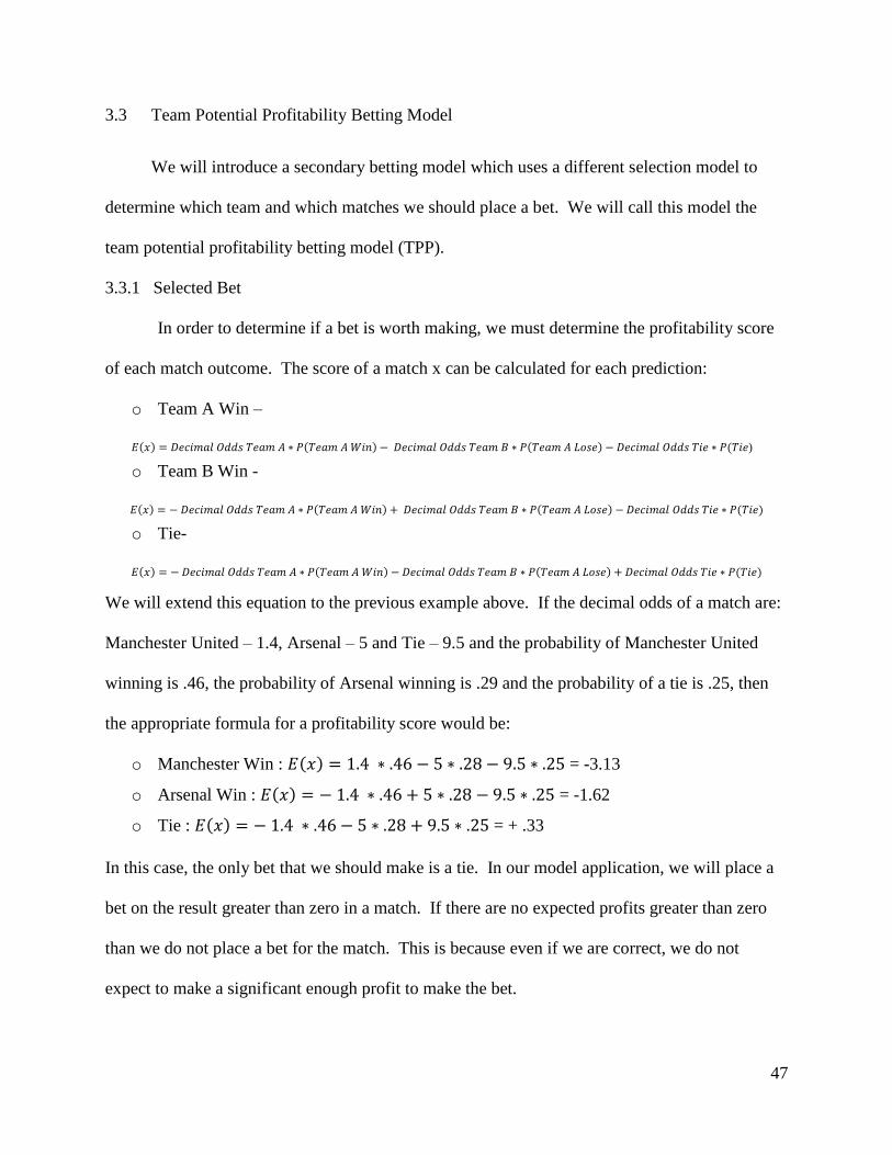
3.3 Team Potential Profitability Betting Model

We will introduce a secondary betting model which uses a different selection model to

determine which team and which matches we should place a bet. We will call this model the

team potential profitability betting model (TPP).

3.3.1 Selected Bet

In order to determine if a bet is worth making, we must determine the profitability score

of each match outcome. The score of a match x can be calculated for each prediction:

o Team A Win –

𝐸(𝑥) = 𝐷𝑒𝑐𝑖𝑚𝑎𝑙 𝑂𝑑𝑑𝑠 𝑇𝑒𝑎𝑚 𝐴 ∗ 𝑃(𝑇𝑒𝑎𝑚 𝐴 𝑊𝑖𝑛) − 𝐷𝑒𝑐𝑖𝑚𝑎𝑙 𝑂𝑑𝑑𝑠 𝑇𝑒𝑎𝑚 𝐵 ∗ 𝑃(𝑇𝑒𝑎𝑚 𝐴 𝐿𝑜𝑠𝑒) − 𝐷𝑒𝑐𝑖𝑚𝑎𝑙 𝑂𝑑𝑑𝑠 𝑇𝑖𝑒 ∗ 𝑃(𝑇𝑖𝑒)

o Team B Win -

𝐸(𝑥) = − 𝐷𝑒𝑐𝑖𝑚𝑎𝑙 𝑂𝑑𝑑𝑠 𝑇𝑒𝑎𝑚 𝐴 ∗ 𝑃(𝑇𝑒𝑎𝑚 𝐴 𝑊𝑖𝑛) + 𝐷𝑒𝑐𝑖𝑚𝑎𝑙 𝑂𝑑𝑑𝑠 𝑇𝑒𝑎𝑚 𝐵 ∗ 𝑃(𝑇𝑒𝑎𝑚 𝐴 𝐿𝑜𝑠𝑒) − 𝐷𝑒𝑐𝑖𝑚𝑎𝑙 𝑂𝑑𝑑𝑠 𝑇𝑖𝑒 ∗ 𝑃(𝑇𝑖𝑒)

o Tie-

𝐸(𝑥) = − 𝐷𝑒𝑐𝑖𝑚𝑎𝑙 𝑂𝑑𝑑𝑠 𝑇𝑒𝑎𝑚 𝐴 ∗ 𝑃(𝑇𝑒𝑎𝑚 𝐴 𝑊𝑖𝑛) − 𝐷𝑒𝑐𝑖𝑚𝑎𝑙 𝑂𝑑𝑑𝑠 𝑇𝑒𝑎𝑚 𝐵 ∗ 𝑃(𝑇𝑒𝑎𝑚 𝐴 𝐿𝑜𝑠𝑒) + 𝐷𝑒𝑐𝑖𝑚𝑎𝑙 𝑂𝑑𝑑𝑠 𝑇𝑖𝑒 ∗ 𝑃(𝑇𝑖𝑒)

We will extend this equation to the previous example above. If the decimal odds of a match are:

Manchester United – 1.4, Arsenal – 5 and Tie – 9.5 and the probability of Manchester United

winning is .46, the probability of Arsenal winning is .29 and the probability of a tie is .25, then

the appropriate formula for a profitability score would be:

o Manchester Win : 𝐸(𝑥) = 1.4 ∗ .46 − 5 ∗ .28 − 9.5 ∗ .25 = -3.13

o Arsenal Win : 𝐸(𝑥) = − 1.4 ∗ .46 + 5 ∗ .28 − 9.5 ∗ .25 = -1.62

o Tie : 𝐸(𝑥) = − 1.4 ∗ .46 − 5 ∗ .28 + 9.5 ∗ .25 = + .33

In this case, the only bet that we should make is a tie. In our model application, we will place a

bet on the result greater than zero in a match. If there are no expected profits greater than zero

than we do not place a bet for the match. This is because even if we are correct, we do not

expect to make a significant enough profit to make the bet.

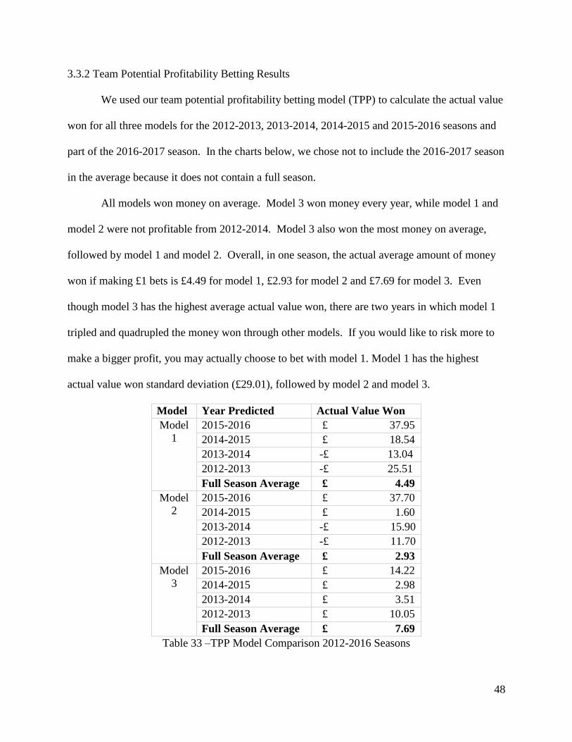
48

3.3.2 Team Potential Profitability Betting Results

We used our team potential profitability betting model (TPP) to calculate the actual value

won for all three models for the 2012-2013, 2013-2014, 2014-2015 and 2015-2016 seasons and

part of the 2016-2017 season. In the charts below, we chose not to include the 2016-2017 season

in the average because it does not contain a full season.

All models won money on average. Model 3 won money every year, while model 1 and

model 2 were not profitable from 2012-2014. Model 3 also won the most money on average,

followed by model 1 and model 2. Overall, in one season, the actual average amount of money

won if making £1 bets is £4.49 for model 1, £2.93 for model 2 and £7.69 for model 3. Even

though model 3 has the highest average actual value won, there are two years in which model 1

tripled and quadrupled the money won through other models. If you would like to risk more to

make a bigger profit, you may actually choose to bet with model 1. Model 1 has the highest

actual value won standard deviation (£29.01), followed by model 2 and model 3.

Model Year Predicted Actual Value Won

Model

1

2015-2016 £ 37.95

2014-2015 £ 18.54

2013-2014 -£ 13.04

2012-2013 -£ 25.51

Full Season Average £ 4.49

Model

2

2015-2016 £ 37.70

2014-2015 £ 1.60

2013-2014 -£ 15.90

2012-2013 -£ 11.70


Model

3

2015-2016 £ 14.22

2014-2015 £ 2.98

2013-2014 £ 3.51

2012-2013 £ 10.05


Table 33 –TPP Model Comparison 2012-2016 Seasons

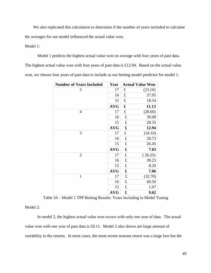
49

We also replicated this calculation to determine if the number of years included to calculate

the averages for our model influenced the actual value won.

Model 1:

Model 1 predicts the highest actual value won on average with four years of past data.

The highest actual value won with four years of past data is £12.94. Based on the actual value

won, we choose four years of past data to include as our betting model predictor for model 1.

Number of Years Included Year Actual Value Won

5 17 £ (23.10)

16 £ 37.95

15 £ 18.54

AVG £ 11.13

4 17 £ (28.60)

16 £ 39.08

15 £ 28.35

AVG £ 12.94

3 17 £ (34.10)

16 £ 28.73

15 £ 26.45

AVG £ 7.03

2 17 £ ( 26.25)

16 £ 39.23

15 £ 8.20

AVG £ 7.06

1 17 £ (32.70)

16 £ 60.50

15 £ 1.07

AVG £ 9.62

Table 34 – Model 1 TPP Betting Results: Years Including in Model Tuning

Model 2:

In model 2, the highest actual value won occurs with only one year of data. The actual

value won with one year of past data is £8.11. Model 2 also shows are large amount of

variability in the returns. In most cases, the most recent seasons return was a large loss but the

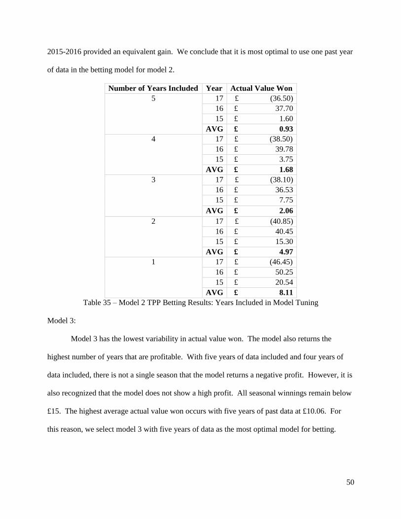
50

2015-2016 provided an equivalent gain. We conclude that it is most optimal to use one past year

of data in the betting model for model 2.


5 17 £ (36.50)

16 £ 37.70

15 £ 1.60

AVG £ 0.93

4 17 £ (38.50)

16 £ 39.78

15 £ 3.75

AVG £ 1.68

3 17 £ (38.10)

16 £ 36.53

15 £ 7.75

AVG £ 2.06

2 17 £ (40.85)

16 £ 40.45

15 £ 15.30

AVG £ 4.97

1 17 £ (46.45)

16 £ 50.25

15 £ 20.54

AVG £ 8.11

Table 35 – Model 2 TPP Betting Results: Years Included in Model Tuning

Model 3:

Model 3 has the lowest variability in actual value won. The model also returns the

highest number of years that are profitable. With five years of data included and four years of

data included, there is not a single season that the model returns a negative profit. However, it is

also recognized that the model does not show a high profit. All seasonal winnings remain below

£15. The highest average actual value won occurs with five years of past data at £10.06. For

this reason, we select model 3 with five years of data as the most optimal model for betting.

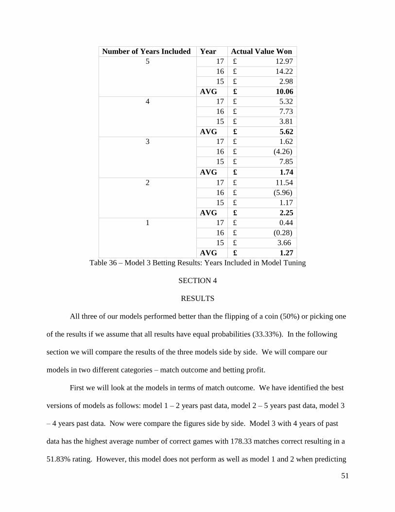
51


5 17 £ 12.97

16 £ 14.22

15 £ 2.98

AVG £ 10.06

4 17 £ 5.32

16 £ 7.73

15 £ 3.81

AVG £ 5.62

3 17 £ 1.62

16 £ (4.26)

15 £ 7.85

AVG £ 1.74

2 17 £ 11.54

16 £ (5.96)

15 £ 1.17

AVG £ 2.25

1 17 £ 0.44

16 £ (0.28)

15 £ 3.66

AVG £ 1.27

Table 36 – Model 3 Betting Results: Years Included in Model Tuning

SECTION 4

RESULTS

All three of our models performed better than the flipping of a coin (50%) or picking one

of the results if we assume that all results have equal probabilities (33.33%). In the following

section we will compare the results of the three models side by side. We will compare our

models in two different categories – match outcome and betting profit.

First we will look at the models in terms of match outcome. We have identified the best

versions of models as follows: model 1 – 2 years past data, model 2 – 5 years past data, model 3

– 4 years past data. Now were compare the figures side by side. Model 3 with 4 years of past

data has the highest average number of correct games with 178.33 matches correct resulting in a

51.83% rating. However, this model does not perform as well as model 1 and 2 when predicting

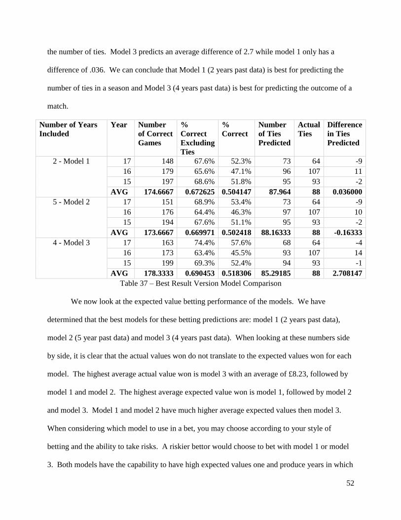
52

the number of ties. Model 3 predicts an average difference of 2.7 while model 1 only has a

difference of .036. We can conclude that Model 1 (2 years past data) is best for predicting the

number of ties in a season and Model 3 (4 years past data) is best for predicting the outcome of a

match.

Number of Years

Included

Year Number

of Correct

Games

%

Correct

Excluding

Ties

%

Correct

Number

of Ties

Predicted

Actual

Ties

Difference

in Ties

Predicted

2 - Model 1 17 148 67.6% 52.3% 73 64 -9

16 179 65.6% 47.1% 96 107 11

15 197 68.6% 51.8% 95 93 -2

AVG 174.6667 0.672625 0.504147 87.964 88 0.036000

5 - Model 2 17 151 68.9% 53.4% 73 64 -9

16 176 64.4% 46.3% 97 107 10

15 194 67.6% 51.1% 95 93 -2

AVG 173.6667 0.669971 0.502418 88.16333 88 -0.16333

4 - Model 3 17 163 74.4% 57.6% 68 64 -4

16 173 63.4% 45.5% 93 107 14

15 199 69.3% 52.4% 94 93 -1

AVG 178.3333 0.690453 0.518306 85.29185 88 2.708147

Table 37 – Best Result Version Model Comparison

We now look at the expected value betting performance of the models. We have

determined that the best models for these betting predictions are: model 1 (2 years past data),

model 2 (5 year past data) and model 3 (4 years past data). When looking at these numbers side

by side, it is clear that the actual values won do not translate to the expected values won for each

model. The highest average actual value won is model 3 with an average of £8.23, followed by

model 1 and model 2. The highest average expected value won is model 1, followed by model 2

and model 3. Model 1 and model 2 have much higher average expected values then model 3.

When considering which model to use in a bet, you may choose according to your style of

betting and the ability to take risks. A riskier bettor would choose to bet with model 1 or model

3. Both models have the capability to have high expected values one and produce years in which

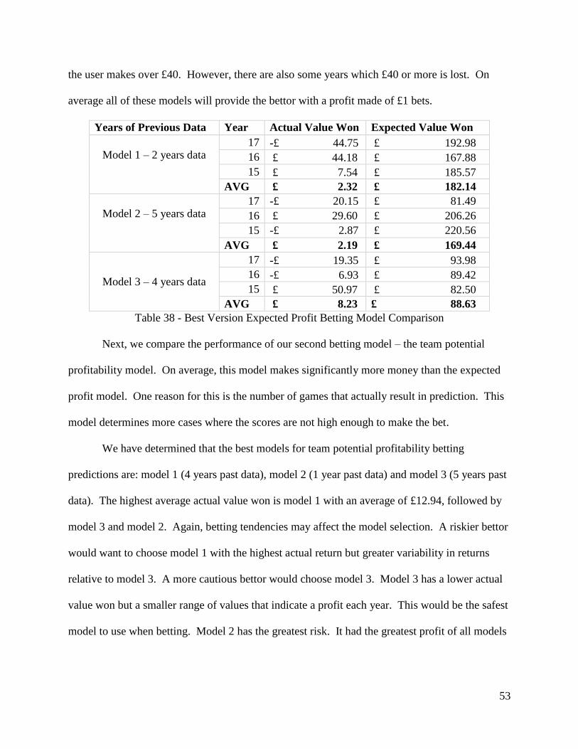
53

the user makes over £40. However, there are also some years which £40 or more is lost. On

average all of these models will provide the bettor with a profit made of £1 bets.

Years of Previous Data Year Actual Value Won Expected Value Won

Model 1 – 2 years data 17 -£ 44.75 £ 192.98

16 £ 44.18 £ 167.88

15 £ 7.54 £ 185.57

AVG £ 2.32 £ 182.14

Model 2 – 5 years data 17 -£ 20.15 £ 81.49

16 £ 29.60 £ 206.26

15 -£ 2.87 £ 220.56

AVG £ 2.19 £ 169.44

Model 3 – 4 years data

17 -£ 19.35 £ 93.98

16 -£ 6.93 £ 89.42

15 £ 50.97 £ 82.50

AVG £ 8.23 £ 88.63

Table 38 - Best Version Expected Profit Betting Model Comparison

Next, we compare the performance of our second betting model – the team potential

profitability model. On average, this model makes significantly more money than the expected

profit model. One reason for this is the number of games that actually result in prediction. This

model determines more cases where the scores are not high enough to make the bet.

We have determined that the best models for team potential profitability betting

predictions are: model 1 (4 years past data), model 2 (1 year past data) and model 3 (5 years past

data). The highest average actual value won is model 1 with an average of £12.94, followed by

model 3 and model 2. Again, betting tendencies may affect the model selection. A riskier bettor

would want to choose model 1 with the highest actual return but greater variability in returns

relative to model 3. A more cautious bettor would choose model 3. Model 3 has a lower actual

value won but a smaller range of values that indicate a profit each year. This would be the safest

model to use when betting. Model 2 has the greatest risk. It had the greatest profit of all models

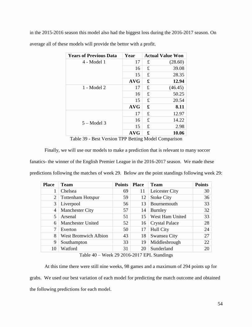
54

in the 2015-2016 season this model also had the biggest loss during the 2016-2017 season. On

average all of these models will provide the bettor with a profit.

Years of Previous Data Year Actual Value Won

4 - Model 1 17 £ (28.60)

16 £ 39.08

15 £ 28.35

AVG £ 12.94

1 - Model 2 17 £ (46.45)

16 £ 50.25

15 £ 20.54

AVG £ 8.11

5 – Model 3

17 £ 12.97

16 £ 14.22

15 £ 2.98

AVG £ 10.06

Table 39 - Best Version TPP Betting Model Comparison

Finally, we will use our models to make a prediction that is relevant to many soccer

fanatics- the winner of the English Premier League in the 2016-2017 season. We made these

predictions following the matches of week 29. Below are the point standings following week 29:

Place Team Points Place Team Points

1 Chelsea 69 11 Leicester City 30

2 Tottenham Hotspur 59 12 Stoke City 36

3 Liverpool 56 13 Bournemouth 33

4 Manchester City 57 14 Burnley 32

5 Arsenal 51 15 West Ham United 33

6 Manchester United 52 16 Crystal Palace 28

7 Everton 50 17 Hull City 24

8 West Bromwich Albion 43 18 Swansea City 27

9 Southampton 33 19 Middlesbrough 22

10 Watford 31 20 Sunderland 20

Table 40 – Week 29 2016-2017 EPL Standings

At this time there were still nine weeks, 98 games and a maximum of 294 points up for

grabs. We used our best variation of each model for predicting the match outcome and obtained

the following predictions for each model.

55

Place Model 1 (4 Years Data) Model 2 (1 Year Data) Model 3 (5 Year Data)

1 Chelsea Tottenham Chelsea

2 Tottenham Chelsea Tottenham

3 Man City Man City Liverpool

4 Liverpool Liverpool Arsenal

5 Arsenal Arsenal Man City

6 Man United Man United Man United

7 Everton Southampton Everton

8 Leicester Leicester Leicester

9 Southampton Everton Southampton

10 West Brom West Ham West Brom

11 West Ham Burnley Watford

12 Bournemouth West Brom Stoke

13 Swansea Watford West Ham

14 Stoke Hull Bournemouth

14 Watford Swansea Swansea

16 Crystal Palace Stoke Hull

17 Burnley Bournemouth Crystal Palace

18 Middlesbrough Middlesbrough Burnley

19 Hull Crystal Palace Middlesbrough

20 Sunderland Sunderland Sunderland

Table 41 – Predicted 2016-2017 EPL Standings by Model

The result predictions differ slightly for each model. Model 2 predicts that Tottenham

will upset Chelsea to take the title.

Previously, we concluded that model 3 with 5 years of past data is best for determining

outcomes in a match. Therefore, we predict that the final league results will be as follows:

Place Team Points Place Team Points

1 Chelsea 99 11 Watford 46

2 Tottenham 89 12 Stoke 45

3 Liverpool 87 13 West Ham 45

4 Arsenal 84 14 Bournemouth 41

5 Man City 82 15 Swansea 40

6 Man United 81 16 Hull 39

7 Everton 60 17 Crystal Palace 37

8 Leicester 57 18 Burnley 35

9 Southampton 55 19 Middlesbrough 29

10 West Brom 47 20 Sunderland 29

Table 42 – Final Predicted 2016-2017 EPL Standings

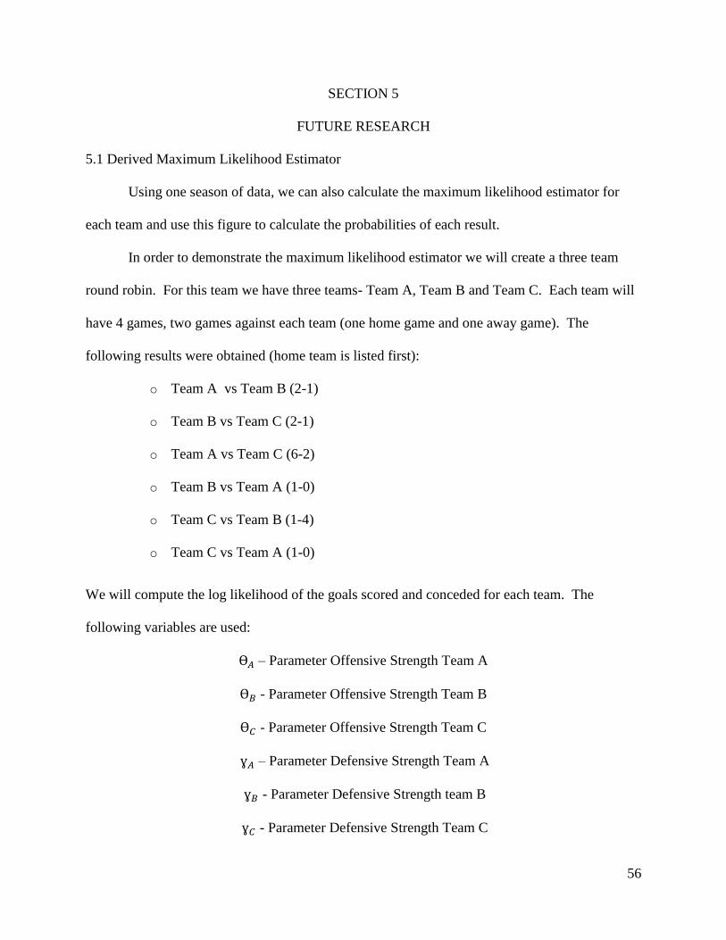
56

SECTION 5

FUTURE RESEARCH

5.1 Derived Maximum Likelihood Estimator

Using one season of data, we can also calculate the maximum likelihood estimator for

each team and use this figure to calculate the probabilities of each result.

In order to demonstrate the maximum likelihood estimator we will create a three team

round robin. For this team we have three teams- Team A, Team B and Team C. Each team will

have 4 games, two games against each team (one home game and one away game). The

following results were obtained (home team is listed first):

o Team A vs Team B (2-1)

o Team B vs Team C (2-1)

o Team A vs Team C (6-2)

o Team B vs Team A (1-0)

o Team C vs Team B (1-4)

o Team C vs Team A (1-0)

We will compute the log likelihood of the goals scored and conceded for each team. The

following variables are used:

ϴ𝐴 – Parameter Offensive Strength Team A

ϴ𝐵 - Parameter Offensive Strength Team B

ϴ𝐶 - Parameter Offensive Strength Team C

ɣ𝐴 – Parameter Defensive Strength Team A

ɣ𝐵 - Parameter Defensive Strength team B

ɣ𝐶 - Parameter Defensive Strength Team C

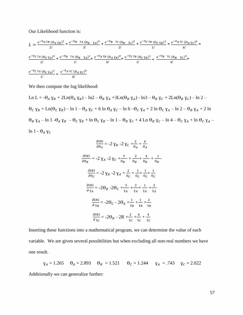
57

Our Likelihood function is:

𝐿 =𝑒−ϴ𝐴 ɣ𝐵 (ϴ𝐴 ɣ𝐵)2

2! *

𝑒−ϴ𝐵 ɣ𝐴 (ϴ𝐵 ɣ𝐴)3

3! *

𝑒−ϴ𝐵 ɣ𝐶 (ϴ𝐵 ɣ𝐶)2

2! *

𝑒−ϴ𝐶 ɣ𝐵 (ϴ𝐶 ɣ𝐵)1

1! *

𝑒−ϴ𝐴 ɣ𝐶 (ϴ𝐴 ɣ𝐶)6

6! *

𝑒−ϴ𝐶 ɣ𝐴 (ϴ𝐶 ɣ𝐴)2

2! *

𝑒−ϴ𝐵 ɣ𝐴 (ϴ𝐵 ɣ𝐴)1

1!*

𝑒−ϴ𝐴 ɣ𝐵 (ϴ𝐴 ɣ𝐵)0

0!*

𝑒−ϴ𝐶 ɣ𝐵 (ϴ𝐶 ɣ𝐵)1

1!∗

𝑒−ϴ𝐵 ɣ𝐶 (ϴ𝐵 ɣ𝐶)4

4!*

𝑒−ϴ𝐶 ɣ𝐴 (ϴ𝐶 ɣ𝐴)1

1!∗

𝑒−ϴ𝐴 ɣ𝐶 (ϴ𝐴 ɣ𝐶)0

0!

We then compute the log likelihood:

Ln L = -ϴ𝐴 ɣ𝐵 + 2Ln(ϴ𝐴 ɣ𝐵) – ln2 – ϴ𝐵 ɣ𝐴 +3Ln(ϴ𝐵 ɣ𝐴) - ln3 – ϴ𝐵 ɣ𝐶 + 2Ln(ϴ𝐵 ɣ𝐶) – ln 2 –

ϴ𝐶 ɣ𝐵 + Ln(ϴ𝐶 ɣ𝐵) – ln 1 – ϴ𝐴 ɣ𝐶 + 6 ln ϴ𝐴 ɣ𝐶 – ln 6 –ϴ𝐶 ɣ𝐴 + 2 ln ϴ𝐶 ɣ𝐴 – ln 2 – ϴ𝐵 ɣ𝐴 + 2 ln

ϴ𝐵 ɣ𝐴 – ln 1 -ϴ𝐴 ɣ𝐵 – ϴ𝐶 ɣ𝐵 + ln ϴ𝐶 ɣ𝐵 – ln 1 – ϴ𝐵 ɣ𝐶 + 4 Ln ϴ𝐵 ɣ𝐶 – ln 4 – ϴ𝐶 ɣ𝐴 + ln ϴ𝐶 ɣ𝐴 –

ln 1 - ϴ𝐴 ɣ𝐶

𝜕𝑙𝑁𝑙

𝜕ϴ𝐴 = -2 ɣ𝐵 -2 ɣ𝐶 +

2

ϴ𝐴 +

6

ϴ𝐴

𝜕𝑙𝑁𝑙

𝜕ϴ𝐵 = -2 ɣ𝐴 -2 ɣ𝐶 +

3

ϴ𝐵 +

2

ϴ𝐵 +

4

ϴ𝐵 +

1

ϴ𝐵

𝜕𝑙𝑁𝑙

𝜕ϴ𝐶 = -2 ɣ𝐵 -2 ɣ𝐴 +

2

ϴ𝐶 +

1

ϴ𝐶+

1

ϴ𝐶+

1

ϴ𝐶

𝜕𝑙𝑁𝑙

𝜕 ɣ𝐴 = -2ϴ𝐵 -2ϴ𝐶 +

3

ɣ𝐴 +

2

ɣ𝐴 +

1

ɣ𝐴 +

2

ɣ𝐴

𝜕𝑙𝑁𝑙

𝜕 ɣ𝐵 = -2ϴ𝐶 - 2ϴ𝐴 +

1

ɣ𝐵 +

1

ɣ𝐵 +

2

ɣ𝐵

𝜕𝑙𝑁𝑙

𝜕 ɣ𝐶 = -2ϴ𝐵 - 2R +

2

ɣ𝐶 +

6

ɣ𝐶 +

4

ɣ𝐶

Inserting these functions into a mathematical program, we can determine the value of each

variable. We are given several possibilities but when excluding all non-real numbers we have

one result.

ɣ𝐴 = 1.265 ϴ𝐴 = 2.893 ϴ𝐵 = 1.521 ϴ𝐶 = 1.244 ɣ𝐴 = .743 ɣ𝐶 = 2.022

Additionally we can generalize further:

58

𝜕𝑙𝑁𝑙

𝜕ϴ𝑖 (Partial Goals Scored) = − ∑ ɣ𝑜𝑝𝑝𝑜𝑠𝑖𝑡𝑖𝑜𝑛 + (𝑡𝑜𝑡𝑎𝑙 𝑔𝑜𝑎𝑙𝑠 𝑠𝑐𝑜𝑟𝑒𝑑)𝑖 *

1

ϴ𝑖

𝜕𝑙𝑁𝑙

𝜕 ɣ𝑖 (Partial Goals Allowed) = − ∑ ϴ𝑜𝑝𝑝𝑜𝑠𝑖𝑡𝑖𝑜𝑛 + (𝑡𝑜𝑡𝑎𝑙 𝑔𝑜𝑎𝑙𝑠 𝑎𝑙𝑙𝑜𝑤𝑒𝑑)𝑖 *

1

ɣ𝑖

We can calculate the maximum likelihood estimator of goals allowed for each team by

subtracting the sum of the attacking variables for each opposing team in each match from

number of goals conceded multiplied by the reciprocal of the defending variable for the desired

team.

We can calculate the maximum likelihood estimator of goals scored for each team by

subtracting the sum of the defensive variables for each opposing team in each match from

number of goals scored multiplied by 1 over the attacking variable for the desired team.

In order to calculate the MLE’s, we entered the generalized form of each equation into

Mathematica. Unfortunately, Mathematica could not calculate the maximum likelihood

estimators identified as individual variables in the set of forty equations. In future research we

hope to identify a better way to find these calculations so these figures can be applied in the

model.

5.2 Model Enhancements

In the future, there are several different topics we can explore to improve our model:

1. Inclusion of new variables - There are many variables that play a role in a soccer

match. In future research we can look further into these variables to determine if they

play a significant role in predicting the number of goals that a team concedes and

scores. These variables may be a valuable addition to the model and may respond

well to weighted averages based on their significance.

2. Seasonal/ Weekly Modifications - The English Premier League lasts from August to

May. In a ten months’ time span, many changes can occur. We can see that our

59

model results in the first half of 2016-2017 were better than the model results from

the first three quarters of the season. This indicates that the model may be better at

predicting earlier in the season. One reason for this could be the time of the results

integrated in the model. As the season progresses, the team dynamics change even

more from the data that we use to calculate the probabilities. In future research, we

can look further into the models performance throughout the season. There may be

some models that perform better at different times in the year. Also, as we move later

in the year, we may want to apply all current team data that we have from past

matches within the season in addition to all previous games. We must be careful not

to do this too soon because games in the current season will have an extremely large

proportional weight if done before a significant amount of the season is complete.

3. Extended Analysis - While we extended our research to include five years of data,

this is only a small percentage of the total seasons for the English Premier League.

We can obtain another twenty years of data to test our models. A bigger data set

would give us more concrete results and confidence in our model selection. This

would also help us see possible patterns of relegation/ promotion teams or teams that

consistently remain in the league.

4. 2016-2017 Season Conclusion - We have also made several predictions for the 2016-

2017 season. In the future we can evaluate these predictions and if they were correct.

We can analyze the final team placement prediction to determine if we were correct.

Based on how close we are to the actual team standings, we may choose to extend

this model to the end of the season placement predictions and bets. We can also look

at the remaining regular season match results to determine if the effectiveness of all

60

models improve as more games are played and we have the same data set size as past

seasons.

5. Further Analysis of Betting Models

a. Expected Value Model – The expected value betting model did not perform as

well as expected. One of the main weaknesses of the model was the amount

of games that the model placed bets on. We can look to improve our model

by determining the best expected profit cut off point. If we increase the

expected profit that we expect from each match we bet on, then we will place

less bets, improving the quality and profitability of our predictions. Along

with this, we can also determine if there are cases in which we should bet on

more than one team in a match.

b. Team Potential Profitability Model - We have identified and described a new

model which we call the team potential profitability betting model. We

stumbled across the creation of this model by chance. This model has

produced successful results but we are unsure of the full mathematical

reasoning that comes behind it. In future research, we hope to expand this

analysis to further identify the success of the model. After identifying this

success, we can potentially improve the model to make it even better.

61

REFERENCES

[1] Ebner, Sarah. "History And Time Are Key To Power Of Football, Says Premier League

Chief | The Times". The Times. N.p., 2016. Web. 14 Nov. 2016.

[2] Kunz, Mattihias. "Big Count". FIFA Magazine. N.p., 2016. Web. 14 Nov. 2016.

[3] Snyder, Jeffery. What Actually Wins Soccer Matches: Prediction Of The 2011-2012 Premier

League For Fun And Profi. 1st ed. 2013. Web. 14 Nov. 2016.

[4] "Premier League Competition Format & History | Premier League". Premierleague.com.

N.p., 2016. Web. 14 Nov. 2016.

[5] Patrick, Seb. "10 Things You Should Know About The English Premier League | BBC

America". BBC America. N.p., 2016. Web. 14 Nov. 2016.

[6] Goddard, John. "Regression Models For Forecasting Goals And Match Results In

Association Football". International Journal of Forecasting 21.2 (2005): 331-340. Web.

[7] Karlis, Dimitris and Ioannis Ntzoufras. "Analysis Of Sports Data By Using Bivariate Poisson

Models". Journal of the Royal Statistical Society: Series D (The Statistician) 52.3 (2003): 381-

393. Web.

[8] Maher, Michael J. "Modelling association football scores." Statistica Neerlandica 36.3

(1982): 109-118.

[9] Yoshimoto, Hisayuki. Maximum Likeihood Estimator. 1st ed. 2008. Web. 14 Nov. 2016.

[10] "Predicting Football Results With Poisson Regression Pt. 1 | Opisthokonta.Net".

Opisthokonta.net. N.p., 2016. Web. 14 Nov. 2016.

62

[11] "Soccer Goal Probabilities: Poisson Vs Actual Distribution - Annabet.Com Blog".

AnnaBet.com Blog. N.p., 2016. Web. 14 Nov. 2016.

[12] McHale, Ian and Phil Scarf. "Cite A Website - Cite This For Me". Salford.ac.uk. N.p., 2016.

Web. 18 Nov. 2016.

[13] Hamilton, Howard. "Goal Scoring Probability Over The Course Of A Football Match |

Soccermetrics Research, LLC". Soccermetrics.net. N.p., 2016. Web. 18 Nov. 2016.

[14] Clarke, Stephen R., and John M. Norman. "Home ground advantage of individual clubs in

English soccer." The Statistician (1995): 509-521.

[15] England Football Results Betting Odds | Premiership Results & Betting Odds. Football-

data.co.uk. 2017. Available at: http://www.football-data.co.uk/englandm.php. Accessed April

11, 2017.

[16] Johnson B. Sports Betting Odds - Explanation of How They Work. Gamblingsitesorg. 2017.

Available at: https://www.gamblingsites.org/sports-betting/beginners-guide/odds/. Accessed

April 11, 2017.

[17] About Us. Helpbet365com. 2017. Available at: https://help.bet365.com/en/about-us.

Accessed April 21, 2017.

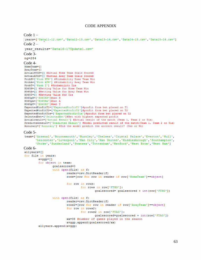
63

CODE APPENDIX

Code 1 –

Code 2 –

Code 3-

Code 4-

Code 5-

Code 6-

64

Code 7-

Code 8-

Code 9-

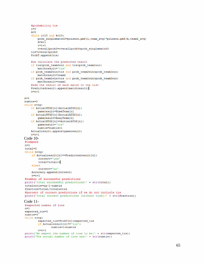
65

Code 10-

Code 11-

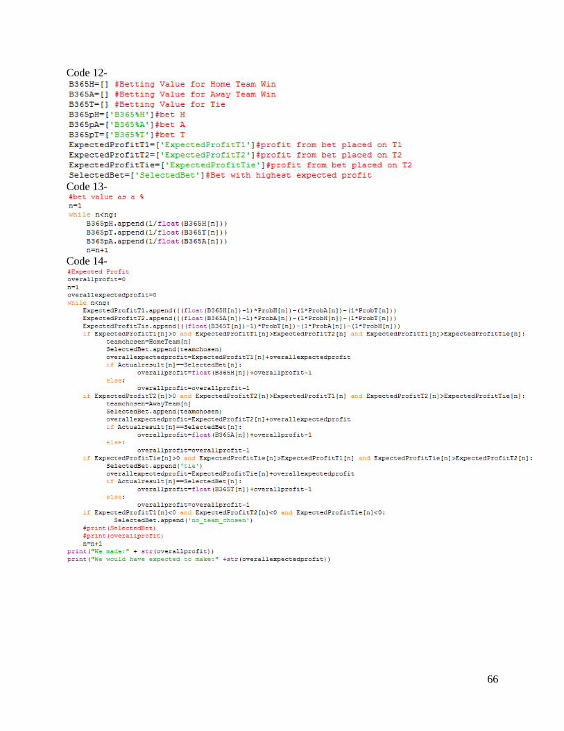
66

Code 12-

Code 13-

Code 14-

Senior Research PREDICTING THE RESULT OF …efriedma/research/boldrin.pdf1.1 Soccer in England ......

Documents

Transcript of Senior Research PREDICTING THE RESULT OF …efriedma/research/boldrin.pdf1.1 Soccer in England ......