Semimartingale approximation of fractional Brownian motion and its applications
11
Computers and Mathematics with Applications 61 (2011) 1844–1854 Contents lists available at ScienceDirect Computers and Mathematics with Applications journal homepage: www.elsevier.com/locate/camwa Semimartingale approximation of fractional Brownian motion and its applications Nguyen Tien Dung Department of Mathematics, Fpt University, No 8 Ton That Thuyet, Cau Giay, Hanoi, Viet Nam article info Article history: Received 24 January 2010 Received in revised form 17 January 2011 Accepted 8 February 2011 Keywords: Fractional Brownian motion Stochastic integrals Semimartingale Black–Scholes model abstract The aim of this paper is to provide a semimartingale approximation of a fractional stochastic integration. This result leads us to approximate the fractional Black–Scholes model by a model driven by semimartingales, and a European option pricing formula is found. © 2011 Elsevier Ltd. All rights reserved. 1. Introduction The fractional Brownian motion (fBm) with Hurst index H ∈ (0, 1) is a centered Gaussian process defined by W H,(1) t = ∫ t 0 K 1 (t , s)dW s , (1.1) where W is a standard Brownian motion and the kernel K 1 (t , s), t ≥ s, is given by K 1 (t , s) = C H [ t H− 1 2 s H− 1 2 (t − s) H− 1 2 − H − 1 2 ∫ t s u H− 3 2 s H− 1 2 (u − s) H− 1 2 du ] , where C H is a coefficient depending only on H. Another form of fractional Brownian motion is Liouville fractional Brownian motion (LfBm) [1,2], where the kernel K 1 (t , s) is replaced by K 2 (t , s) = (t − s) H− 1 2 , that is a stochastic process defined by W H,(2) t := ∫ t 0 (t − s) α dW s , α = H − 1 2 . In [3] Mandelbrot has given a relation between W H,(1) t and W H,(2) t W H,(1) t = 1 Γ (1 + α) U t + W H,(2) t , (1.2) where U t = 0 −∞ (t − s) α − (−s) α dW s is a process of absolutely continuous trajectories. E-mail addresses: [email protected], [email protected]. 0898-1221/$ – see front matter © 2011 Elsevier Ltd. All rights reserved. doi:10.1016/j.camwa.2011.02.013
-
Upload
nguyen-tien-dung -
Category
Documents
-
view
213 -
download
1
Transcript of Semimartingale approximation of fractional Brownian motion and its applications
Computers and Mathematics with Applications 61 (2011) 1844–1854
Contents lists available at ScienceDirect
Computers and Mathematics with Applications
journal homepage: www.elsevier.com/locate/camwa
Semimartingale approximation of fractional Brownian motion and itsapplicationsNguyen Tien DungDepartment of Mathematics, Fpt University, No 8 Ton That Thuyet, Cau Giay, Hanoi, Viet Nam
a r t i c l e i n f o
Article history:Received 24 January 2010Received in revised form 17 January 2011Accepted 8 February 2011
Keywords:Fractional Brownian motionStochastic integralsSemimartingaleBlack–Scholes model
a b s t r a c t
The aim of this paper is to provide a semimartingale approximation of a fractionalstochastic integration. This result leads us to approximate the fractional Black–Scholesmodel by a model driven by semimartingales, and a European option pricing formula isfound.
© 2011 Elsevier Ltd. All rights reserved.
1. Introduction
The fractional Brownian motion (fBm) with Hurst index H ∈ (0, 1) is a centered Gaussian process defined by
WH,(1)t =
∫ t
0K1(t, s)dWs, (1.1)
whereW is a standard Brownian motion and the kernel K1(t, s), t ≥ s, is given by
K1(t, s) = CH
[tH−
12
sH−12(t − s)H−
12 −
H −
12
∫ t
s
uH−32
sH−12
(u − s)H−12 du
],
where CH is a coefficient depending only on H .Another form of fractional Brownian motion is Liouville fractional Brownian motion (LfBm) [1,2], where the kernel
K1(t, s) is replaced by K2(t, s) = (t − s)H−12 , that is a stochastic process defined by
WH,(2)t :=
∫ t
0(t − s)αdWs, α = H −
12.
In [3] Mandelbrot has given a relation betweenWH,(1)t andWH,(2)
t
WH,(1)t =
1Γ (1 + α)
Ut + WH,(2)
t, (1.2)
where Ut = 0−∞
(t − s)α − (−s)α
dWs is a process of absolutely continuous trajectories.
E-mail addresses: [email protected], [email protected].
0898-1221/$ – see front matter© 2011 Elsevier Ltd. All rights reserved.doi:10.1016/j.camwa.2011.02.013
N.T. Dung / Computers and Mathematics with Applications 61 (2011) 1844–1854 1845
It is well known that in the case where the Hurst index H =12 , the process WH (WH
= WH,(1)t or WH,(2)
t ) is a standardBrownian motion and where H =
12 ,W
H is neither a semimartingale nor a Markov process. Hence, the stochastic calculusdevelopedby Itô cannot be applied. In this paperweuse the pathwise stochastic integration,which is introduced by Zähle [4],to consider the following fractional version of the Black–Scholes (FB–S) model:
Bond price:
dBt = rBtdt; B0 = 1 (1.3)
Stock price:
dSt = µStdt + σ StdWHt , (1.4)
where S0 is a positive real number and WHt is either a fBm or a LfBm. The coefficients r, µ, σ are assumed to be constants
symbolizing the riskless interest rate, the drift of the stock and its volatility, respectively.The arbitrage in the (FB–S) model based on pathwise integration was studied by Shiryayev [5] for the case of H > 1
2 .Cheridito [6] proved a surprising result that, for Hurst parameters H ∈
34 , 1
the mixed process MH,ε
t = WH,(1)t + εW 1
t isequivalent to a martingale εW 1
t , as long as the standard Brownian motionW 1t is independent ofWH,(1)
t . He observes that
Cov(MH,εt ,MH,ε
s ) = ε2 min(t, s) + Cov(WH,(1)t ,WH,(1)
s ).
Hence, MH,εt is an a.s. continuous centered Gaussian process that has up to ε2 the same covariance structure as (WH,(1)
t ).Cheridito [6] verbally explains how this fact shows that if the stock price process in (FB–S) model fits empirical data, thenso does
dSt = µStdt + σ StdWH,(1)t + εσ StdW 1
t ; S0 > 0 (1.5)
for ε > 0 small enough.It is obvious that mixed model (1.5) is arbitrage-free and complete. For a fixed value ε, one can price asset with respect
to the unique martingale measure Qε and get at time t = 0
C0(ε) = EQε
S0 exp(µT + σ(WH,(1)
T + εW 1T )) − e−rTK
+= BS(0, S0, σε),
where BS(0, S0, σε) denotes the Black–Scholes price of a call option on a stock with initial price S0 and volatility σε. Asε → 0, the mixed model (1.5) approaches the model (1.4), and the option price tends to
C0 = limε→0
BS(0, S0, σε) = (S0 − e−rTK)+, (1.6)
that is, all randomness is eliminated. Cheridito [6] explains this peculiarity by the possibility that traders can act arbitrarilyfast and hence immediately exploit the predictability of the model (1.5). Thereby, they remove the random character bymeans of a suitable trading strategy.
However, we can see that the mixed model (1.5) contains one random source more than the original model (1.4). Thismeans that the dynamism of (1.5) is different from that of (1.4) even for arbitrarily small ε.
In [7–9], T. H. Thao has proved that a LfBm can be approximated in L2(Ω) by semimartingales. We developed this resultby showing thatWH
t can be approximated in Lp(Ω) by semimartingales
WH,εt =
∫ t
0K(t + ε, s)dWs, ε > 0,
where K(t, s) equals to either K1(t, s) or K2(t, s). This fact leads us to the following approximation model for stock priceprocess
dSεt = µSε
t dt + σ Sεt dW
H,εt ; S0 > 0. (1.7)
This model driven by semimartingales has the same random source as original (FB–S) model. We want also to emphasizethat our approximation results is true for all H > 1
2 .This paper is organized as follows: In Section 2, we state some basic facts about a semimartingale approximation of
fractional processes and the generalized Stieltjes integral. In Section 3, our key result is stated in Theorem 3.1 that thefractional stochastic integral can be approximated by the stochastic integrationwith respect to semimartingales. In Section 4,the absence of arbitrage and semimartingale approximation of the Black–Scholes model are proved, the Black–Scholesequation is found as well.
1846 N.T. Dung / Computers and Mathematics with Applications 61 (2011) 1844–1854
2. Preliminaries
Let us at first define the following stochastic process for every ε > 0
WH,εt =
∫ t
0K(t + ε, s)dWs,
where K(t, s) equals to either K1(t, s) or K2(t, s). We have the following proposition:
Proposition 2.1. I. For every ε > 0,WH,εt is Ft-semimartingale with following decomposition
WH,εt =
∫ t
0K(s + ε, s)dWs +
∫ t
0ϕεs ds, (2.1)
where (Ft , 0 ≤ t ≤ T ) is the natural filtration associated to W.
ϕεs =
∫ s
0∂1K(s + ε, u)dWu,
∂1K(t, s) =∂K(t, s)
∂t.
II. The process WH,εt converges to WH
t in Lp(Ω), p > 0when ε tends to 0. This convergence is uniform with respect to t ∈ [0, T ].
Proof. The proof of part I is as follows: applying stochastic Fubini’s theorem we have∫ t
0ϕεs ds =
∫ t
0
∫ s
0∂1K(s + ε, u)dWuds =
∫ t
0
∫ t
u∂1K(s + ε, u)dsdWu
=
∫ t
0
K(t + ε, u) − K(u + ε, u)
dWu = WH,ε
t −
∫ t
0K(s + ε, s)dWs. (2.2)
Hence, (2.1) follows from (2.2).We are now in a position to prove part II of the proposition. For any p > 0, applying Burkholder–Davis–Gundy inequality
(see, [10]) we get
E|WH,εt − WH
t |p
≤ E∫ t
0
K(t + ε, s) − K(t, s)
dWs
p
≤ cp
∫ t
0
K(t + ε, s) − K(t, s)
2ds p2
, (2.3)
where cp is a finite positive constant and∫ t
0
K(t + ε, s) − K(t, s)
2ds =
∫ t
0K 2(t + ε, s)ds − 2
∫ t
0K(t + ε, s)K(t, s)ds +
∫ t
0K 2(t, s)ds
≤
∫ t+ε
0K 2(t + ε, s)ds − 2
∫ t∧(t+ε)
0K(t + ε, s)K(t, s)ds +
∫ t
0K 2(t, s)ds
= E|WHt+ε − WH
t |2
≤ ε2H . (2.4)
Hence,
E|WH,εt − WH
t |p
≤ cpεpH .
The proof of the proposition is complete.
Corollary 2.1. Let Sεt , St be the solution to Eqs. (1.4), (1.7), respectively. Then Sε
t converges to St in Lp(Ω), p > 0 when ε → 0,provided that H > 1
2 . This convergence is uniform with respect to t ∈ [0, T ].
Proof. Let X1, X2 be two random variables. By Lagrange’s theorem and Hölder’s inequality we have
E|eX1 − eX2 |p ≤ E
(X1 − X2) supmin(X1,X2)≤x≤max(X1,X2)
exp
≤ E|(X1 − X2)e|X1|+|X2||p ≤
E[e2p|X1| + e2p|X2|]E|X1 − X2|
2p 1
2
. (2.5)
N.T. Dung / Computers and Mathematics with Applications 61 (2011) 1844–1854 1847
We recall from [11] that
St = S0eµt+σWHt , Sε
t = S0eµt− 12 σ 2K2(t+ε,t)+σWH,ε
t .
We now apply (2.5) to X1 = −12σ
2K 2(t + ε, t) + σWH,εt , X2 = σWH
t and obtain
E|Sεt − St |p = Sp0e
pµtE|e−12 σ 2K2(t+ε,t)+σWH,ε
t − eσWHt |
p
≤ Sp0epµt
E[e2p|X1| + e2p|X2|]E|X1 − X2|
2p 1
2
. (2.6)
It is obvious that E[e2p|X1| + e2p|X2|] is finite because WH,εt and WH
t are centered Gaussian processes with finite variances in[0, T ]. Moreover, by fundamental inequality (a + b)p ≤ cp(ap + bp), where cp = 1 if 0 < p ≤ 1 and cp = 2p−1 if p > 1
E|X1 − X2|2p
≤ c2p
[E|WH,ε
t − WHt |
2p+
14p
σ 4pK 4p(t + ε, t)]
≤ c2p
ε2pH
+14p
σ 4pε4p
H−
12
. (2.7)
Thus, for 0 < ε < 1, there exists a finite constant C(p, S0, T ) depending only on p, S0 and T such that
E|Sεt − St |p ≤ C(p, S0, T )ε
2pH−
12
. (2.8)
Next, we recall about a generalization of the Stieltjes integral introduced by Zähle [4]. Fix a parameter 0 < λ < 12 , denote
by W 1−λ,∞[0, T ] the space of measurable function g : [0, T ] → R such that
‖g‖1−λ,∞ := sup0≤s<t≤T
|g(t) − g(s)|(t − s)1−λ
+
∫ t
s
|g(y) − g(s)|(y − s)2−λ
dy
< +∞.
Clearly,
C1−λ+ε[0, T ] ⊂ W 1−λ,∞
[0, T ] ⊂ C1−λ[0, T ] ∀ε > 0,
where Cλ[0, T ] denotes the space of Hölder continuous functions of order λ with the norm
‖g‖λ := sup0≤t≤T
|g(t)| + sup0≤s<t≤T
|g(t) − g(s)||t − s|λ
.
We also denote byW λ,1[0, T ] the space of measurable function f : [0, T ] → R such that
‖f ‖λ,1 :=
∫ T
0
|f (s)|sλ
ds +
∫ T
0
∫ t
0
|f (t) − f (s)|(t − s)λ+1
dsdt < ∞.
For the functions f ∈ W λ,1[0, T ], g ∈ W 1−λ,∞
[0, T ], Zähle introduced the generalized Stieltjes integral∫ T
0f (t)dg(t) = (−1)λ
∫ T
0Dλ0+ f (t)D1−λ
T− g(t)dt
defined in terms of the fractional derivative operators
Dλ0+ f (x) =
1Γ (1 − λ)
f (x)xλ
+ λ
∫ x
0
f (x) − f (y)(x − y)λ+1
dy
,
and
D1−λ
T− g(x) =(−1)λ
Γ (1 − λ)
g(x) − g(T )
(T − x)λ+ λ
∫ T
x
g(x) − g(y)(x − y)λ+1
dy
.
Moreover, we have the following estimate for all t ∈ [0, T ]∫ t
0f dg
≤ C(λ)‖f ‖λ,1‖g‖1−λ,∞. (2.9)
If f ∈ Cλ[0, T ] and g ∈ Cµ
[0, T ] with λ + µ > 1, it is proved by Zähle that the integral t0 f dg coincides with the
Riemann–Stieltjes integral.
1848 N.T. Dung / Computers and Mathematics with Applications 61 (2011) 1844–1854
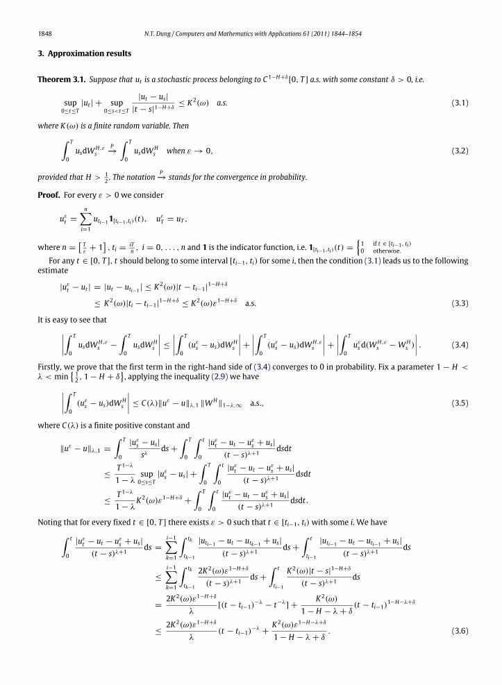
3. Approximation results
Theorem 3.1. Suppose that ut is a stochastic process belonging to C1−H+δ[0, T ] a.s. with some constant δ > 0, i.e.
sup0≤t≤T
|ut | + sup0≤s<t≤T
|ut − us|
|t − s|1−H+δ≤ K 2(ω) a.s. (3.1)
where K(ω) is a finite random variable. Then∫ T
0usdWH,ε
sP−→
∫ T
0usdWH
s when ε → 0, (3.2)
provided that H > 12 . The notation
P−→ stands for the convergence in probability.
Proof. For every ε > 0 we consider
uεt =
n−i=1
uti−11[ti−1,ti)(t), uεT = uT ,
where n = T
ε+ 1
, ti =
iTn , i = 0, . . . , n and 1 is the indicator function, i.e. 1[ti−1,ti)(t) =
1 if t ∈ [ti−1, ti)0 otherwise.
For any t ∈ [0, T ], t should belong to some interval [ti−1, ti) for some i, then the condition (3.1) leads us to the followingestimate
|uεt − ut | = |ut − uti−1 | ≤ K 2(ω)|t − ti−1|
1−H+δ
≤ K 2(ω)|ti − ti−1|1−H+δ
≤ K 2(ω)ε1−H+δ a.s. (3.3)
It is easy to see that∫ T
0usdWH,ε
s −
∫ T
0usdWH
s
≤
∫ T
0(uε
s − us)dWHs
+
∫ T
0(uε
s − us)dWH,εs
+
∫ T
0uεsd(W
H,εs − WH
s )
. (3.4)
Firstly, we prove that the first term in the right-hand side of (3.4) converges to 0 in probability. Fix a parameter 1 − H <λ < min
12 , 1 − H + δ
, applying the inequality (2.9) we have∫ T
0(uε
s − us)dWHs
≤ C(λ)‖uε− u‖λ,1 ‖WH
‖1−λ,∞ a.s., (3.5)
where C(λ) is a finite positive constant and
‖uε− u‖λ,1 =
∫ T
0
|uεs − us|
sλds +
∫ T
0
∫ t
0
|uεt − ut − uε
s + us|
(t − s)λ+1dsdt
≤T 1−λ
1 − λsup
0≤s≤T|uε
s − us| +
∫ T
0
∫ t
0
|uεt − ut − uε
s + us|
(t − s)λ+1dsdt
≤T 1−λ
1 − λK 2(ω)ε1−H+δ
+
∫ T
0
∫ t
0
|uεt − ut − uε
s + us|
(t − s)λ+1dsdt.
Noting that for every fixed t ∈ [0, T ] there exists ε > 0 such that t ∈ [ti−1, ti) with some i. We have∫ t
0
|uεt − ut − uε
s + us|
(t − s)λ+1ds =
i−1−k=1
∫ tk
tk−1
|uti−1 − ut − utk−1 + us|
(t − s)λ+1ds +
∫ t
ti−1
|uti−1 − ut − uti−1 + us|
(t − s)λ+1ds
≤
i−1−k=1
∫ tk
tk−1
2K 2(ω)ε1−H+δ
(t − s)λ+1ds +
∫ t
ti−1
K 2(ω)|t − s|1−H+δ
(t − s)λ+1ds
=2K 2(ω)ε1−H+δ
λ[(t − ti−1)
−λ− t−λ
] +K 2(ω)
1 − H − λ + δ(t − ti−1)
1−H−λ+δ
≤2K 2(ω)ε1−H+δ
λ(t − ti−1)
−λ+
K 2(ω)ε1−H−λ+δ
1 − H − λ + δ. (3.6)

N.T. Dung / Computers and Mathematics with Applications 61 (2011) 1844–1854 1849
Hence,
‖uε− u‖λ,1 ≤
K 2(ω)
1 − H − λ + δ(t − ti−1)
1−H−λ+δ+
2K 2(ω)ε1−H+δ
λ
∫ T
0(t − ti−1)
−λdt +K 2(ω)ε1−H−λ+δ
1 − H − λ + δ→ 0 (3.7)
as ε → 0 because the integral in the right-hand side of (3.7) is finite.It is well known thatWH has (H−η)-Hölder continuous paths for all η ∈ (0,H) (see, [3]), i.e. there exists a finite random
variable Kη(ω) such that
|WHt − WH
s | ≤ Kη(ω)|t − s|H−η∀t, s ∈ [0, T ] a.s.
For 0 < η < λ − (1 − H) we have
‖WH‖1−λ,∞ = sup
0≤s<t≤T
|WH
t − WHs |
(t − s)1−λ+
∫ t
s
|WHy − WH
s |
(y − s)2−λdy
≤ Kη(ω) sup
0≤s<t≤T
(t − s)H+λ−η−1
+
∫ t
s(y − s)H+λ−η−2dy
≤ Kη(ω)TH+λ−η−1
1 +
1H + λ − η − 1
. (3.8)
As a consequence, by combining (3.5), (3.7) and (3.8) the first term in the right-hand side of (3.4) will converge to zeroin probability as ε → 0.
Next, we prove that the second term in the right-hand side of (3.4) converges to zero in L2(Ω) by using the decomposition(2.1).
E∫ T
0(uε
s − us)dWH,εs
2 ≤ E∫ T
0(uε
s − us)K(s + ε, s)dWs
2 + E∫ T
0(uε
s − us)ϕεs ds
2≤
∫ T
0E(uε
s − us)2K 2(s + ε, s)ds + ε2−2H+2δ
∫ T
0E
K 2(ω)ϕεs
2 ds. (3.9)
It is obvious that the first term in the right-hand side of (3.9) converges to zero in L2(Ω) because E(uεs − us)
2≤
E[K 4(ω)]ε2−2H+2δ and K(s + ε, s) → K(s, s) = 0 as ε → 0.Applying the Hölder and the Burkholder–Davis–Gundy inequalities we have
EK 2(ω)ϕε
s
2 ≤E|K(ω)|8
1/2E|
∫ s
0∂1K(s + ε, u)dWu|
41/2
≤ C∫ s
0|∂1K(s + ε, u)|2du,
where C is a finite constant. We recall that
∂1K(t, s) =
CH
tH−12
sH−12(t − s)H−
32 ifWH
t = WH,(1)t ,
H −12
(t − s)H−
32 ifWH
t = WH,(2)t .
There exists C ′ not depending on ε such that
EK 2(ω)ϕε
s
2 ≤ C ′
∫ s
0(s + ε − u)2H−3du =
C ′
2 − 2H[ε2H−2
− (s + ε)2H−2],
and so the second term in the right-hand side of (3.9) converges to zero in L2(Ω).Finally, we prove that the third term in the right-hand side of (3.4) converges to 0.∫ T
0uεsd(W
H,εs − WH
s ) =
n−i=1
uti−1(WH,εti − WH
ti − WH,εti−1
+ WHti−1
) + uT (WH,εT − WH
T )
=
n−i=1
(uti−1 − uti)(WH,εti − WH
ti ) + uT (WH,εT − WH
T ). (3.10)

1850 N.T. Dung / Computers and Mathematics with Applications 61 (2011) 1844–1854
It is obvious that uT (WH,εT − WH
T )L2(Ω)−−−→ 0 becauseWH,ε
TL2(Ω)−−−→ WH
T . Moreover, we have n−i=1
(uti−1 − uti)(WH,εti − WH
ti )
≤ K 2(ω)
n−i=1
|ti−1 − ti|1−H+δ|WH,ε
ti − WHti |, (3.11)
and
En−
i=1
|ti−1 − ti|1−H+δ|WH,ε
ti − WHti | ≤
n−i=1
|ti−1 − ti|1−H+δ
E|WH,ε
ti − WHti |
2 1
2
≤
n−i=1
Tn
1−H+δ
εH
≤
n−i=1
ε1−H+δεH
=
[Tε
+ 1]
ε1+δ→ 0 when ε → 0. (3.12)
Thus, the proof of the theorem is complete.
Remark 3.1. Another approximation approach is given by Androshchuk [12] who proved that for a stochastic processu ∈ C2−2H+δ
[0, T ] ⊂ C1−H+δ[0, T ] a.s. the fractional stochastic integral can be approximated by integrals with respect
to absolutely continuous processes. More applications to finance is introduced by Mishura [13].
4. Applications to fractional Black–Scholes model
Theorem 4.1. Suppose that H ∈ (0, 1). For fixed ε > 0, the approximation models (1.3) and (1.7) has no arbitrage.
Proof. Using (2.1) we can rewrite (1.7) as follows
dSεt = (µ + σϕε
s )Sεt dt + σK(t + ε, t)Sε
t dWt; S0 > 0. (4.1)
From [14, Theorem 12.1.8] we have only to prove that the stochastic process
u(t, ω) :=µ + σϕε
t − rσK(t + ε, t)
satisfies the Novikov’s condition
E[exp
12
∫ T
0u2(t, ω)dt
]< ∞.
The latest inequality holds obviously because ϕεt =
t0 ∂1K(t + ε, u)dWu is a Gaussian process with finite variance.
Thus, the proof of the theorem is complete.
A strategy in this model is a pair of adapted stochastic processes π = (αt , βt), where the processes αt and βt denote thenumber of bonds at time t and number of stock shares held at time t , respectively. Thus, the corresponding wealth processis given by
Vt = αtBt + βtSt ,
where Bt and St are the bond price and stock price at time t , respectively.We make the following assumptions about the strategy π :
(A1) π is a self-financing strategy, i.e.
Vt = V0 +
∫ t
0αsdBs +
∫ t
0βsdSs
where the second integral in the right-hand side is a pathwise integral.(A2) π is a strategy of the following form (Markov-type strategy)
αt = α(t, St), βt = β(t, St).
Next, we will prove that in the class of the Markov-type strategies the wealth process can be considered as a limit ofsemimartingales. Indeed, we have
V εt = α(t, Sε
t )Bt + β(t, Sεt )S
εt

N.T. Dung / Computers and Mathematics with Applications 61 (2011) 1844–1854 1851
or equivalently,
V εt = V0 +
∫ t
0α(s, Sε
s )dBs +
∫ t
0β(s, Sε
s )dSεs
= V0 +
∫ t
0
α(s, Sε
s )rBs + µβ(s, Sεs )S
εs
ds +
∫ t
0σβ(s, Sε
s )Sεs dW
H,εs .
From the semimartingale decomposition (2.1) we obtain
V εt = V0 +
∫ t
0
rα(s, Sε
s )Bs + µβ(s, Sεs )S
εs + σϕε
s β(s, Sεs )S
εs
ds +
∫ t
0σK(s + ε, s)β(s, Sε
s )Sεs dWs (4.2)
which means that V εt is a semimartingale.
Theorem 4.2. Let H > 12 and assume that the self-financing, Markov-type strategy π satisfies the following conditions with
some constants δ1, δ2, δ3 > 0
(C1) |α(t, x) − α(t, y)| ≤ M|x − y|δ1 ∀x, y ∈ R ∀t ∈ [0, T ].(C2) |β(t, x) − β(s, x)| ≤ M|t − s|
12 +δ2 ∀x ∈ R ∀t, s ∈ [0, T ].
(C3) β(t, x) is a differentiable function in x and
|β ′
x(t, x)| ≤ M(1 + |x|δ3) ∀x ∈ R.
Then V εt
P−→ Vt as ε → 0 for any t ∈ [0, T ].
Proof. We have
Vt = V0 +
∫ t
0α(s, Ss)dBs +
∫ t
0β(s, Ss)dSs
= V0 +
∫ t
0
α(s, Ss)rBs + µβ(s, Ss)Ss
ds +
∫ t
0σβ(s, Ss)SsdWH
s ,
V εt = V0 +
∫ t
0α(s, Sε
s )dBs +
∫ t
0β(s, Sε
s )dSεs
= V0 +
∫ t
0
α(s, Sε
s )rBs + µβ(s, Sεs )S
εs
ds +
∫ t
0σβ(s, Sε
s )Sεs dW
H,εs .
Hence,
|V εt − Vt | ≤
∫ t
0
α(s, Sεs ) − α(s, Ss)
r ersds + µ
∫ t
0
β(s, Sεs )S
εs − β(s, Ss)Ss
ds+
∫ t
0σβ(s, Sε
s )Sεs dW
H,εs −
∫ t
0σβ(s, Ss)SsdWH
s
:= I1 + I2 + I3. (4.3)
First, by using Hölder’s inequality and the condition (C1) we get
E[I21 ] ≤
∫ t
0r2 e2rsds
∫ t
0E|α(s, Sε
s ) − α(s, Ss)|2ds
≤rM2(e2rT − 1)
2
∫ t
0E|Sε
s − Ss|2δ1ds. (4.4)
Consequently, Corollary 2.1 implies that I1L2(Ω)−−−→ 0 when ε → 0.
Next, we prove that I2 also converges to 0 in L2(Ω). Indeed, put f (t, x) = β(t, x)x, uεt = f (t, Sε
t ) and ut = f (t, St) then byHölder’s inequality we have
E|uεt − ut |
2≤ E
A(t, x)(Sε
t − St)2
≤E|A(t, x)|4
12E|Sε
t − St |4 12 , (4.5)
where
A(t, x) := supmin(Sε
t ,St )≤x≤max(Sεt ,St )
∂ f (t, x)∂x
.
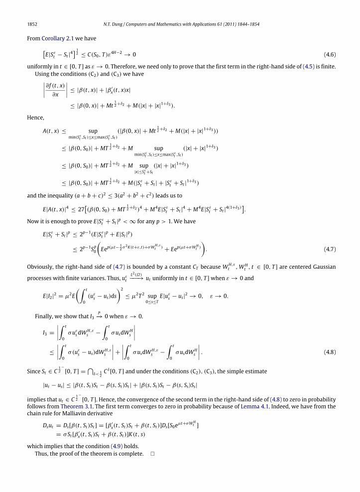
1852 N.T. Dung / Computers and Mathematics with Applications 61 (2011) 1844–1854
From Corollary 2.1 we haveE|Sε
t − St |4 12 ≤ C(S0, T )ε4H−2
→ 0 (4.6)
uniformly in t ∈ [0, T ] as ε → 0. Therefore, we need only to prove that the first term in the right-hand side of (4.5) is finite.Using the conditions (C2) and (C3) we have∂ f (t, x)∂x
≤ |β(t, x)| + |β ′
x(t, x)x|
≤ |β(0, x)| + Mt12 +δ2 + M(|x| + |x|1+δ3).
Hence,
A(t, x) ≤ supmin(Sε
t ,St )≤x≤max(Sεt ,St )
(|β(0, x)| + Mt12 +δ2 + M(|x| + |x|1+δ3))
≤ |β(0, S0)| + MT12 +δ2 + M sup
min(Sεt ,St )≤x≤max(Sε
t ,St )(|x| + |x|1+δ3)
≤ |β(0, S0)| + MT12 +δ2 + M sup
|x|≤Sεt +St
(|x| + |x|1+δ3)
≤ |β(0, S0)| + MT12 +δ2 + M(|Sε
t + St | + |Sεt + St |1+δ3)
and the inequality (a + b + c)2 ≤ 3(a2 + b2 + c2) leads us to
E|A(t, x)|4 ≤ 27(β(0, S0) + MT
12 +δ2)4 + M4E|Sε
t + St |4 + M4E|Sεt + St |4(1+δ3)
.
Now it is enough to prove E|Sεt + St |p < ∞ for any p > 1. We have
E|Sεt + St |p ≤ 2p−1(E|Sε
t |p+ E|St |p)
≤ 2p−1Sp0
Eep(µt− 1
2 σ 2K(t+ε,t)+σWH,εt )
+ Eep(µt+σWHt )
. (4.7)
Obviously, the right-hand side of (4.7) is bounded by a constant CT because WH,εt ,WH
t , t ∈ [0, T ] are centered Gaussian
processes with finite variances. Thus, uεt
L2(Ω)−−−→ ut uniformly in t ∈ [0, T ] when ε → 0 and
E|I2|2 = µ2E∫ t
0(uε
s − us)ds2
≤ µ2T 2 sup0≤s≤T
E|uεs − us|
2→ 0, ε → 0.
Finally, we show that I3P−→ 0 when ε → 0.
I3 =
∫ t
0σuε
sdWH,εs −
∫ t
0σusdWH
s
≤
∫ t
0σ(uε
s − us)dWH,εs
+
∫ t
0σusdWH,ε
s −
∫ t
0σusdWH
s
. (4.8)
Since St ∈ C12
−
[0, T ] =
δ< 12Cδ
[0, T ] and under the conditions (C2), (C3), the simple estimate
|ut − us| ≤ |β(t, St)St − β(s, St)St | + |β(s, St)St − β(s, Ss)Ss|
implies that ut ∈ C12
−
[0, T ]. Hence, the convergence of the second term in the right-hand side of (4.8) to zero in probabilityfollows from Theorem 3.1. The first term converges to zero in probability because of Lemma 4.1. Indeed, we have from thechain rule for Malliavin derivative
Dsut = Ds[β(t, St)St ] = [β ′
x(t, St)St + β(t, St)]Ds[S0eµt+σWHt ]
= σ St [β ′
x(t, St)St + β(t, St)]K(t, s)
which implies that the condition (4.9) holds.Thus, the proof of the theorem is complete.
N.T. Dung / Computers and Mathematics with Applications 61 (2011) 1844–1854 1853
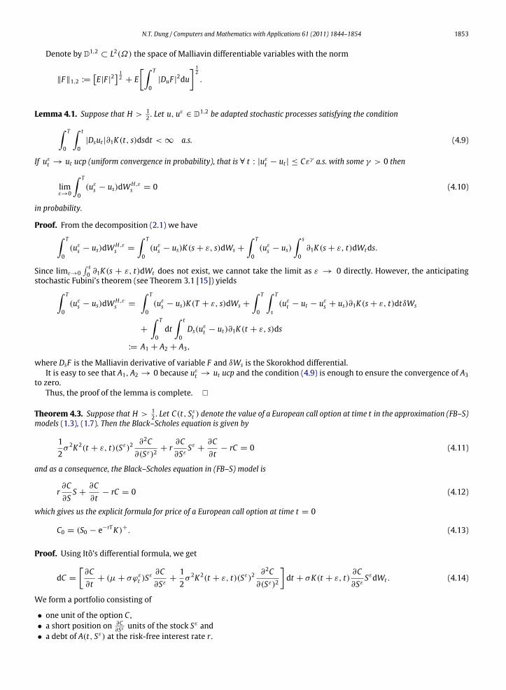
Denote by D1,2⊂ L2(Ω) the space of Malliavin differentiable variables with the norm
‖F‖1,2 :=E|F |
2 12 + E
[∫ T
0|DuF |
2du] 1
2
.
Lemma 4.1. Suppose that H > 12 . Let u, u
ε∈ D1,2 be adapted stochastic processes satisfying the condition∫ T
0
∫ t
0|Dsut |∂1K(t, s)dsdt < ∞ a.s. (4.9)
If uεt → ut ucp (uniform convergence in probability), that is ∀ t : |uε
t − ut | ≤ Cεγ a.s. with some γ > 0 then
limε→0
∫ T
0(uε
s − us)dWH,εs = 0 (4.10)
in probability.
Proof. From the decomposition (2.1) we have∫ T
0(uε
s − us)dWH,εs =
∫ T
0(uε
s − us)K(s + ε, s)dWs +
∫ T
0(uε
s − us)
∫ s
0∂1K(s + ε, t)dWtds.
Since limε→0 s0 ∂1K(s + ε, t)dWt does not exist, we cannot take the limit as ε → 0 directly. However, the anticipating
stochastic Fubini’s theorem (see Theorem 3.1 [15]) yields∫ T
0(uε
s − us)dWH,εs =
∫ T
0(uε
s − us)K(T + ε, s)dWs +
∫ T
0
∫ T
s(uε
t − ut − uεs + us)∂1K(s + ε, t)dtδWs
+
∫ T
0dt
∫ t
0Ds(uε
t − ut)∂1K(t + ε, s)ds
:= A1 + A2 + A3,
where DsF is the Malliavin derivative of variable F and δWs is the Skorokhod differential.It is easy to see that A1, A2 → 0 because uε
t → ut ucp and the condition (4.9) is enough to ensure the convergence of A3to zero.
Thus, the proof of the lemma is complete.
Theorem 4.3. Suppose that H > 12 . Let C(t, Sε
t ) denote the value of a European call option at time t in the approximation (FB–S)models (1.3), (1.7). Then the Black–Scholes equation is given by
12σ 2K 2(t + ε, t)(Sε)2
∂2C∂(Sε)2
+ r∂C∂Sε
Sε+
∂C∂t
− rC = 0 (4.11)
and as a consequence, the Black–Scholes equation in (FB–S) model is
r∂C∂S
S +∂C∂t
− rC = 0 (4.12)
which gives us the explicit formula for price of a European call option at time t = 0
C0 = (S0 − e−rTK)+. (4.13)
Proof. Using Itô’s differential formula, we get
dC =
[∂C∂t
+ (µ + σϕεt )S
ε ∂C∂Sε
+12σ 2K 2(t + ε, t)(Sε)2
∂2C∂(Sε)2
]dt + σK(t + ε, t)
∂C∂Sε
SεdWt . (4.14)
We form a portfolio consisting of
• one unit of the option C ,• a short position on ∂C
∂Sε units of the stock Sε and• a debt of A(t, Sε) at the risk-free interest rate r .
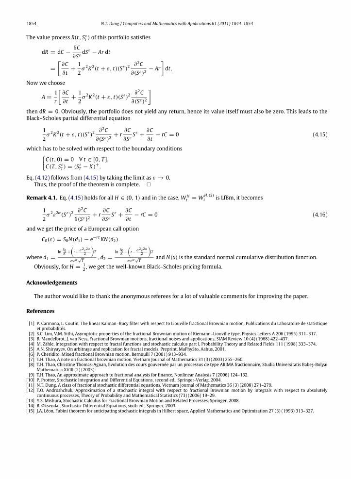
1854 N.T. Dung / Computers and Mathematics with Applications 61 (2011) 1844–1854
The value process R(t, Sεt ) of this portfolio satisfies
dR = dC −∂C∂Sε
dSε− Ar dt
=
[∂C∂t
+12σ 2K 2(t + ε, t)(Sε)2
∂2C∂(Sε)2
− Ar]dt.
Now we choose
A =1r
[∂C∂t
+12σ 2K 2(t + ε, t)(Sε)2
∂2C∂(Sε)2
]then dR = 0. Obviously, the portfolio does not yield any return, hence its value itself must also be zero. This leads to theBlack–Scholes partial differential equation
12σ 2K 2(t + ε, t)(Sε)2
∂2C∂(Sε)2
+ r∂C∂Sε
Sε+
∂C∂t
− rC = 0 (4.15)
which has to be solved with respect to the boundary conditionsC(t, 0) = 0 ∀ t ∈ [0, T ],
C(T , SεT ) = (Sε
T − K)+.
Eq. (4.12) follows from (4.15) by taking the limit as ε → 0.Thus, the proof of the theorem is complete.
Remark 4.1. Eq. (4.15) holds for all H ∈ (0, 1) and in the case,WHt = WH,(2)
t is LfBm, it becomes
12σ 2ε2α(Sε)2
∂2C∂(Sε)2
+ r∂C∂Sε
Sε+
∂C∂t
− rC = 0 (4.16)
and we get the price of a European call option
C0(ε) = S0N(d1) − e−rTKN(d2)
where d1 =
ln S0K +
r+ σ2ε2α
2
T
σεα√T
, d2 =
ln S0K +
r− σ2ε2α
2
T
σεα√T
and N(x) is the standard normal cumulative distribution function.
Obviously, for H =12 , we get the well-known Black–Scholes pricing formula.
Acknowledgements
The author would like to thank the anonymous referees for a lot of valuable comments for improving the paper.
References
[1] P. Carmona, L. Coutin, The linear Kalman–Bucy filter with respect to Liouville fractional Brownian motion, Publications du Laboratoire de statistiqueet probabilités.
[2] S.C. Lim, V.M. Sithi, Asymptotic properties of the fractional Brownian motion of Riemann–Liouville type, Physics Letters A 206 (1995) 311–317.[3] B. Mandelbrot, J. van Ness, Fractional Brownian motions, fractional noises and applications, SIAM Review 10 (4) (1968) 422–437.[4] M. Zähle, Integration with respect to fractal functions and stochastic calculus part I, Probability Theory and Related Fields 111 (1998) 333–374.[5] A.N. Shiryayev, On arbitrage and replication for fractal models, Preprint, MaPhySto, Aahus, 2001.[6] P. Cheridito, Mixed fractional Brownian motion, Bernoulli 7 (2001) 913–934.[7] T.H. Thao, A note on fractional brownian motion, Vietnam Journal of Mathematics 31 (3) (2003) 255–260.[8] T.H. Thao, Christine Thomas-Agnan, Evolution des cours gouvernée par un processus de type ARIMA fractionnaire, Studia Universitatis Babeş-Bolyai
Mathematica XVIII (2) (2003).[9] T.H. Thao, An approximate approach to fractional analysis for finance, Nonlinear Analysis 7 (2006) 124–132.
[10] P. Protter, Stochastic Integration and Differential Equations, second ed., Springer-Verlag, 2004.[11] N.T. Dung, A class of fractional stochastic differential equations, Vietnam Journal of Mathematics 36 (3) (2008) 271–279.[12] T.O. Androshchuk, Approximation of a stochastic integral with respect to fractional Brownian motion by integrals with respect to absolutely
continuous processes, Theory of Probability and Mathematical Statistics (73) (2006) 19–29.[13] Y.S. Mishura, Stochastic Calculus for Fractional Brownian Motion and Related Processes, Springer, 2008.[14] B. Øksendal, Stochastic Differential Equations, sixth ed., Springer, 2003.[15] J.A. Léon, Fubini theorem for anticipating stochastic integrals in Hilbert space, Applied Mathematics and Optimization 27 (3) (1993) 313–327.