Bachelor Thesis

Semi-supervised emotion lexicon expansionwith label propagation and specialized word embeddings

A thesis presented for the degree ofBachelor of Arts in

International Studies in Computational Linguistics

Mario Giulianelli

July 2017

Supervised by Dr Daniel de Kok

Seminar fur SprachwissenschaftUniversitat Tubingen

Germany

arX

iv:1

708.

0391

0v1

[cs

.CL

] 1

3 A

ug 2

017

The main contribution

of this Bachelor thesis

will soon be reported in

a standalone paper.

1 Introduction

As the amount of online data increases, new methods are continuously developed tomake sense of the available information. The Web and social networks have allowed any-one with an Internet connection to contribute to this enormous, freely available database.The data is mostly unorganized and text is probably the most abundant unstructured re-source. On online platforms, users express their opinions and share their experiences,thus they generate a complex network of mutual influence. Reviews of goods and ser-vices, political views and commentaries, as well as recommendations of job applicantsexemplify how Web content can impact the decision-making process of consumers, vot-ers, companies, and other organizations (Pang et al., 2008). Therefore, it is not surprisingthat sentiment analysis and opinion mining are active areas of academic and industrialresearch nowadays.

The term sentiment analysis lacks a unified definition. Generally, it refers to the au-tomatic detection of a user’s evaluative or emotional attitude toward a topic, as it is ex-pressed in a text. More commonly, the meaning of sentiment is restricted to the polarity(or valence) of a text, i.e. whether the text is positive, negative, or neutral (Mohammad,2015).

When a service or a product are the target of customer reviews, blog posts, or tweets,it may be sufficiently informative to determine the valence of the text. However, in manycases, expanding such binary—or ternary—categories to a set of chosen emotions yieldshigher explanatory power. From this claim rises the field of emotion classification, oremotion analysis, or non-binary sentiment analysis.

As in the case of binary sentiment analysis, there exist two main approaches to auto-matically extract affectual orientation: lexicon-based and corpus-based. The lexicon-based approach considers the orientation of single words and phrases in the docu-ment and it requires dictionaries of words labeled with the emotion—or emotions—they evoke. The corpus-based approach can be seen as a supervised classification task.Hence, it requires emotion-annotated corpora. The performance of a statistical emo-tion classifier is typically good in the domain the classifier is trained on, but it canbe mediocre when applied to other domains. Such classifiers lack generalizing powerbecause their only source of information is the corpus they learn from, i.e. they arecontext-dependent. Consequently, the lexicon-based approach is often preferred as itprovides higher context-independence (Taboada et al., 2011). An important limitation tothe lexicon-based method is still the small size of the available lexical resources, whichhas a positive effect on precision at the cost of low recall. We propose a new lexiconexpansion routine that addresses this shortcoming.

In the proposed framework, emotion-specific word embeddings are learned from acorpus of texts labeled with six basic emotions (anger, disgust, fear, joy, sadness, andsurprise). The derived vector space model is used to expand an existing emotion lexiconvia a semi-supervised label propagation algorithm.

This thesis has multiple contributions. It introduces a novel variant of the Label Prop-agation algorithm that is tailored to distributed word representations. It applies batchgradient descent to accelerate the optimization of label propagation and to make theoptimization feasible for large graphs. It proposes a reproducible method for emotionlexicon expansion, which can be leveraged to improve the accuracy of an emotion clas-sifier.

An emotion-labeled corpus and an emotion lexicon are the two necessary resourcesfor our method. As for the former, we use the Hashtag Emotion Corpus (Mohammad andKiritchenko, 2015), a collection of tweets labeled with Ekman’s six basic emotions (Ek-

1

man, 1992). The lexical resource we employ is the NRC Emotion Lexicon (Mohammadand Turney, 2013).

The first step of our approach is to use the corpus as source of supervision for adeep neural network model. In particular, the core architecture is a Long Short TermMemory (LSTM) recurrent network (Hochreiter and Schmidhuber, 1997). The deepmodel learns emotion-specific representations of words via backpropagation, where theemotion-specificity of a word vector refers to the ability to encode affectual orientationand strength in a subset of its dimensions. Next, the specialized embeddings are em-ployed to build a semantic-similarity graph. The emotion lexicon is expanded using ournovel variation of the Label Propagation algorithm (Zhu and Ghahramani, 2002).

The rest of this thesis is structured as follows: we begin with a review of related workin the areas of emotion classification and lexicon expansion, and with a description ofthe statistical approaches that can be used to learn task-specific continuous representa-tions (Section 2). Then, the proposed lexicon expansion method and the optimizationof specialized word embeddings are presented (Section 3). Section 4 presents an anal-ysis of the employed resources. The experiments performed to learn emotion-specificembeddings and to expand the lexicon are reported in Section 5 along with intrinsic andextrinsic evaluation in an emotion classification task (Section 6). Section 7 concludesand proposes new research ideas.

The software related to this paper is open-source and available at https://github.com/Procope/emo2vec.

2 Related work

2.1 Emotion classificationAmong the various areas of opinion mining, sentiment analysis is probably the mostthoroughly explored. While sentiment analysis refers to the automatic detection of auser’s affectual attitude toward a topic, more commonly, the goal of the field is to deter-mine the polarity of phrases, sentences, and documents (polarity or valence annotation).Hence, text can be typically classified as positive, negative, or neutral. It is, however,common to extend the number of valence classes to at least five: this finer-grained anal-ysis additionally includes very positive and very negative in the polarity scale.

While sentiment analysis is an active and useful research area, it can only prove lim-itedly informative as it essentially maps text to a one-dimensional space. Indeed theusual range of valence is [−1, 1]. Another possible goal of sentiment analysis is to stillautomatically detect a user’s affectual orientation, but with the difference that text is as-signed to one or more classes of emotions. By increasing the number of dimensions usedto represent emotional orientation, such opinion mining methods gain in interpretativeand explanatory power. We refer to this extended problem as emotion classification oremotion analysis. There are two possibility for the classification of texts into emotioncategories: multinomial classification, where the classifier outputs a probability distri-bution over all emotions, and multi-label classification, where the classifier returns aprobability for each emotion.

An important milestone for emotion analysis was the SemEval-2007 Affective Texttask. The motivation for the task was that there seems to be a connection between lex-ical semantics and the way we verbally express emotions (Strapparava and Mihalcea,2007). In particular, it was argued that emotional orientation and strength of a textare determined potentially by all words that compose it, though, disputedly, in unevenamount. Therefore, expressions that appear to be neutral can also convey affective mean-ing as they might be semantically related to emotional concepts. Consider the following

2

tweets:

(1) I want cake. I bet we don’t have any.

(2) Saddened by the terrifying events in Virginia.

(1) conveys frustration, which, in terms of basic emotions, could be translated into thelabels anger and / or sadness although its constituents appear to be neutral. Similarly, (2)clearly expresses an affectual orientation but the NRC Emotion Lexicon does not containsadden, saddened nor terrify, terrifying. The claim that all words potentially conveyaffective meaning is inspirational for our work and it provides a rationale for lexiconexpansion (Section 2.4 and 3.2): since possibly all terms in a document contribute to itsaffective content, employing lexica of, at best, 15,000 types is a serious limitation.

The lexicon-based approach relies on labeled dictionaries to calculate the emotionalorientation of a text based on the words and phrases that constitute it (Turney, 2002). Adisadvantage of dictionaries is that they contain direct affective words, i.e. words thatrefer directly to affective states. In contrast, indirect affective words only have a weakconnection to emotional concepts that depends on the context they appear in (Strapparavaet al., 2006). To give an example, an American professional baseball player, who wascriticized for his unsatisfactory performance, publicly stated:

(3) I am going to have a monster year.

The indirect affective word monster is clearly used as a positive modifier, but context isrequired to make such an inference.

Finally, consider the following headline whose emotional orientation is rather positive.

(4) Beating poverty in a small way.

It contains the direct affective words beating and poverty, which are labeled as expres-sions of anger, disgust, fear, and sadness in the NRC Emotion Lexicon (Section 2.2).Sentence (4) is an example of how lexicon-based methods cannot correctly analyze com-positionality (beating poverty). Negations and sarcasm are other such issues, which canonly be solved adding rules, chunking, or parsing.

The use of dictionaries is not the only approach to emotion analysis. As it happens,there is another relevant method to address this task. The automatic extraction of affec-tual orientation can be viewed as a supervised classification problem, which requires anemotion-annotated data set and a statistical learning algorithm. This is often referred toas the corpus-based approach (Pang et al., 2002).

In the area of corpus-based methods, researchers have proposed different systemsthat, having access to contextual information, have the potential to address the issuesof lexicon-based techniques: basic compositionality, negation, and cases of obvious sar-casm.

Two corpus-based systems participated in the SemEval-2007 Affective Text task: UAand SWAT. UA uses Weighted Pointwise Mutual Information (PMI) to compute emotionscores. The distribution of emotions and the distribution of nouns, verbs, adjectives, andadverbs are obtained via statistical analysis of texts crawled from Web search engines.Then, given the set of words Wt in a text t, and an emotion word e, PMI is defined as:

PMI (t, e) =fr (Wt ∩ {e})fr (Wt) fr (e)

Additionally, an associative score between content words and emotions is estimated to

3

weight the PMI score.An even more traditional supervised system is SWAT. Based on a unigram model,

SWAT additionally uses a thesaurus to obtain the synonyms of emotion label words (e.g.the synonym of joy, or surprise). Finally, Strapparava and Mihalcea (2008) proposed aNaıve Bayes classifier trained on mood-annotated blog posts.

While UA and SWAT were the corpus-based systems participating in the SemEval-2007 Affective Text task, UPAR7 is an example of the lexicon-based counterpart.UPAR7 can be described as a linguistic approach. It parses a document and uses the re-sulting dependency graph to reconstruct what is said about the main subject. All words inthe document have emotion scores based on SentiWordNet (Esuli and Sebastiani, 2007)and WordNet Affect (Strapparava et al., 2004), enriched with lexical contrast and accen-tuation. A higher weight is given to the score of the main subject, while the other weightsare computed considering linguistic categories such as negation and modal verbs.

There exist as well combinations of the two main approaches. Strapparava and Mihal-cea (2008) used, on the one hand, lexical resources (WordNet Affect) to annotate synsetsrepresenting emotions and moods. For each emotion, a list of words is generated by thecorresponding synset. On the other hand, the British National Corpus is fed into a vari-ation of Latent Semantic Analysis (LSA) to obtain a vector space model, where words,documents, and synsets are represented as vectors. Documents and synsets are mappedinto the vector space by computing the sum over the normalized LSA vectors of all thewords comprised in them. Once an emotion is represented in the LSA vector space, de-termining affective orientation is essentially a matter of computing a similarity measurebetween an input word, paragraph, or text, and the prototypical emotion vectors. Thiswas the best performing system at SemEval-2007, which suggests that lexical resourcesand corpora are complementary sources of information.

Yang et al. (2015) combined the two main learning methods in a unified co-trainingframework applied to valence annotation, obtaining state-of-the-art results on variousEnglish and Chinese datasets. Indeed, further studies (Kennedy and Inkpen, 2006; An-dreevskaia and Bergler, 2008; Qiu et al., 2009) showed that the performance of lexicon-and corpus-based approaches is complementary in terms of precision and recall. Thelexicon-based method yields higher recall at the cost of low precision, as it is likely totag an instance with label l whenever an emotion word related to l is found—i.e. even ifthe text is neutral or rather evocative of another emotion. In contrast, supervised learn-ing systems tend to perform poorly in terms of recall—since their vocabulary is limitedto the types seen in the training data—but they reach higher precision scores as labelsare assigned in a more fine-grained manner (Yang et al., 2015)—after all, most traininginstances have a considerable neutral content (Section 4).

None of the systems participating to SemEval-2007 reached an accuracy similar tothat of sentiment analysis methods. This is possibly the reason why it is hard to find lit-erature about alternative approaches to those used in the Affective Text task, and why asimilar task was not proposed in successive editions of SemEval. However, the inter-annotator agreement studies conducted by (Strapparava and Mihalcea, 2007) for theSemEval headlines corpus, remind us that there is an upper bound to the accuracy ofemotion classification algorithms, namely human accuracy. Table 1 shows the agree-ment scores in terms of Pearson correlation, as they can be found in the original paper. Iftrained annotators agree with a simple average r of 53.67 (the frequency-based averager is 43), it is plausible that untrained respondents would show an even lower level ofagreement. In Section 6.3 we describe the results of a survey that tests the ability of anaverage untrained person to classify short paragraphs into emotions.

4

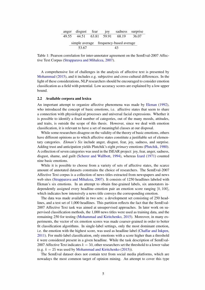
anger disgust fear joy sadness surprise49.55 44.51 63.81 59.91 68.19 36.07

simple average frequency-based average53.67 43

Table 1: Pearson correlation for inter-annotator agreement on the SemEval-2007 Affec-tive Text Corpus (Strapparava and Mihalcea, 2007).

A comprehensive list of challenges in the analysis of affective text is presented byMohammad (2015), and it includes e.g. subjective and cross-cultural differences. In thelight of these considerations, NLP researchers should be encouraged to consider emotionclassification as a field with potential. Low accuracy scores are explained by a low upperbound.

2.2 Available corpora and lexica

An important attempt to organize affective phenomena was made by Ekman (1992),who introduced the concept of basic emotions, i.e. affective states that seem to sharea connection with physiological processes and universal facial expressions. Whether itis possible to identify a fixed number of categories, out of the many moods, attitudes,and traits, is outside the scope of this thesis. However, since we deal with emotionclassification, it is relevant to have a set of meaningful classes at our disposal.

While some researchers disagree on the validity of the theory of basic emotions, othershave different opinions as to which affective states constitute a justifiable set of elemen-tary categories. Ekman’s Six include anger, disgust, fear, joy, sadness, and surprise.Adding trust and anticipation yields Plutchik’s eight primary emotions (Plutchik, 1980).A collection of seven categories was used in the ISEAR project: joy, fear, anger, sadness,disgust, shame, and guilt (Scherer and Wallbott, 1994), whereas Izard (1971) countednine basic emotions.

While it is possible to choose from a variety of sets of affective states, the scarceamount of annotated datasets constrains the choice of researchers. The SemEval-2007Affective Text corpus is a collection of news titles extracted from newspapers and newsweb sites (Strapparava and Mihalcea, 2007). It consists of 1250 headlines labeled withEkman’s six emotions. In an attempt to obtain fine-grained labels, six annotators in-dependently assigned every headline–emotion pair an emotion score ranging [0, 100],which indicates how intensively a news title conveys the corresponding emotion.

The data was made available in two sets: a development set consisting of 250 head-lines, and a test set of 1,000 headlines. This partition reflects the fact that the SemEval-2007 Affective Text task was aimed at unsupervised approaches. In later work on su-pervised classification methods, the 1,000 news titles were used as training data, and theremaining 250 for testing (Mohammad and Kiritchenko, 2015). Moreover, in many ex-periments, the vector of six emotion scores was made coarser-grained in order to betterfit classification algorithms. In single-label settings, only the most dominant emotion,i.e. the emotion with the highest score, was used as headline label (Chaffar and Inkpen,2011). For multi-label classification, only emotions with a score higher than a thresholdk were considered present in a given headline. While the task description of SemEval-2007 Affective Text indicates k = 50, other researchers set the threshold to a lower value(e.g. k = 25 was used by Mohammad and Kiritchenko (2015)).

The SemEval dataset does not contain text from social media platforms, which arenowadays the most common target of opinion mining. An attempt to cover this type

5

of content was made by Mohammad and Kiritchenko (2015), who created a corpus oftweets (Twitter posts) leveraging the use of hashtags (i.e. words immediately precededby a hash symbol which mostly serve to signal the topic of Twitter posts, as well as othersorts of metadata such as the tweeter’s mood). The Hashtag Emotion Corpus consists ofabout 21,000 tweets annotated with one out of the six emotions proposed by Ekman.

Other corpora were compiled with sentence-level annotation. Sentences extractedfrom 22 fairy tales were annotated by Alm et al. (2005) with 5 emotions (joy, fear, sad-ness, surprise, and anger-disgust). Aman and Szpakowicz (2007) annotated about 5,000sentences drawn from blog posts with Ekman’s six emotions and a neutral category.Neviarouskaya et al. (2009) chose the nine emotion categories proposed by Izard (and aneutral one) to label 1,000 sentences extracted from stories on a variety of topics.

Lexical resources are not abundant either. WordNet Affect is a word-emotion asso-ciation lexicon consisting of 1,536 terms (Strapparava et al., 2004). In occasion of theSemEval Affective Text task, a set of 152 words extracted from WordNet Affect wasmade available for optional use. The Hashtag Emotion Lexicon contains 11,418 lem-mas automatically obtained from the Hashtag Emotion Corpus (Mohammad and Kir-itchenko, 2015). Each word-emotion pair comes with a real-valued association score,namely the Strength of Association (SoA) score between a word w and emotion e:SoA(w, e) = PMI(w, e) − PMI(w,¬e). While the three above lexica use Ekman’sSix, the NRC Emotion Lexicon (Mohammad and Turney, 2013) combines the eight pri-mary emotions proposed by Plutchik with the positive and negative polarities, for a totalof ten possible labels. The NRC Emotion Lexicon includes 14,182 English words. It wasmanually created via crowdsourcing and uses binary word-emotion association scores.

2.3 Learning task-specific continuous representations

Supervised methods of statistical learning require input data to be represented by fea-tures. In NLP there are many ways to encode words, sentences, and paragraphs. While itwas common to hand-engineer linguistically motivated features, the field now prefers au-tomatic feature generation as it does not demand domain expertise nor extensive manualwork, and it allows to define language-independent techniques and models.

A simple yet common way to represent words are one-hot vectors, which can, ingeneral, be used to encode categorical features. Each word is represented as a booleanvector whose length is equal to the size of the vocabulary: if a word is at position iin the vocabulary, only the ith dimension of the word vector is set to 1. As a result,words are represented by large, sparse vectors which can be fed into various statisticallearning algorithms, such as linear classifiers. Although the one-hot representation canbe improved by using e.g. counts instead of boolean values, it can encode virtually noinformation about the relation between words and their similarities.

As deep learning started to regain popularity, alternative encodings resurged. Sparsevectors were largely replaced by dense continuous representations, word embeddings,which have proved effective in multiple NLP tasks such as parsing, language modeling,named entity recognition, machine translation, and word sense disambiguation.

Particularly interesting for our research is the field of statistical language modeling,which successfully uses distributed representations of words as a paradigm (Rumelhartet al., 1988). Unlike one-hot vectors, word-embeddings do not represent words in iso-lation. They rather exploit the context of a word to learn its syntactic and semanticproperties.

Mikolov et al. (2013a) proposed two architectures for efficiently estimating vector rep-resentations of words from large corpora: the Continuous Bag-of-Words model (CBOW)

6

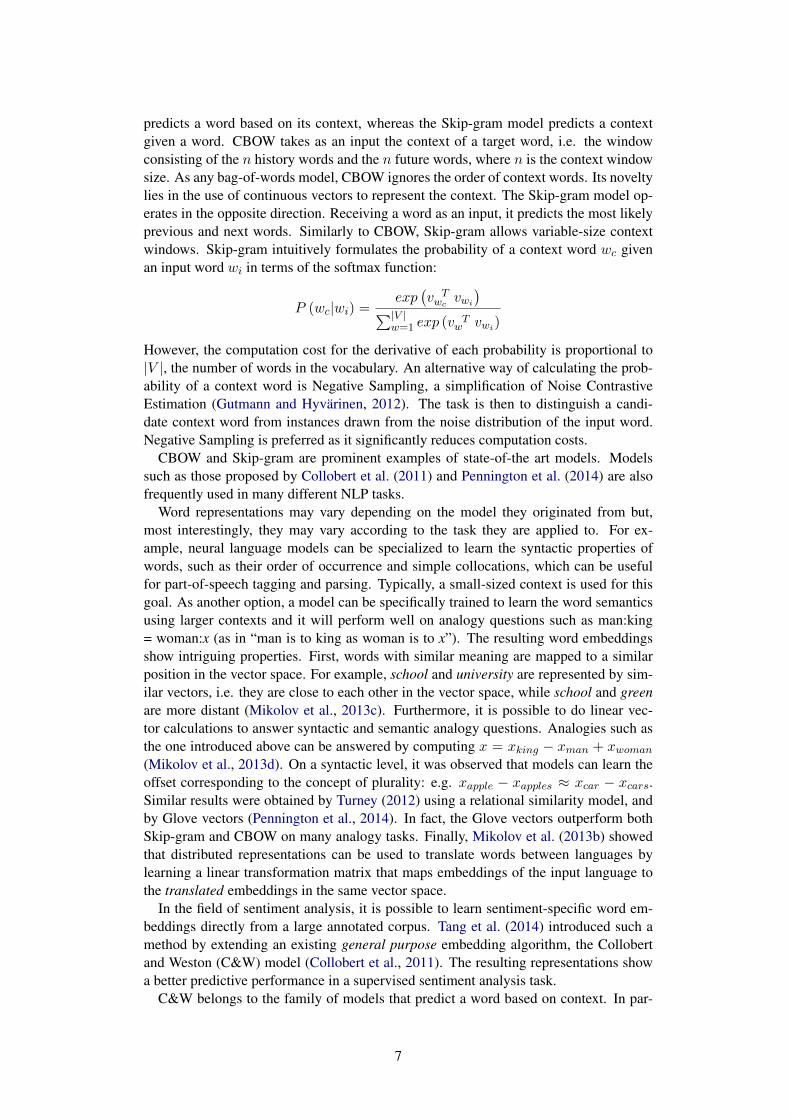
predicts a word based on its context, whereas the Skip-gram model predicts a contextgiven a word. CBOW takes as an input the context of a target word, i.e. the windowconsisting of the n history words and the n future words, where n is the context windowsize. As any bag-of-words model, CBOW ignores the order of context words. Its noveltylies in the use of continuous vectors to represent the context. The Skip-gram model op-erates in the opposite direction. Receiving a word as an input, it predicts the most likelyprevious and next words. Similarly to CBOW, Skip-gram allows variable-size contextwindows. Skip-gram intuitively formulates the probability of a context word wc givenan input word wi in terms of the softmax function:

P (wc|wi) =exp

(v Twc

vwi

)∑|V |w=1 exp (v T

w vwi)

However, the computation cost for the derivative of each probability is proportional to|V |, the number of words in the vocabulary. An alternative way of calculating the prob-ability of a context word is Negative Sampling, a simplification of Noise ContrastiveEstimation (Gutmann and Hyvarinen, 2012). The task is then to distinguish a candi-date context word from instances drawn from the noise distribution of the input word.Negative Sampling is preferred as it significantly reduces computation costs.

CBOW and Skip-gram are prominent examples of state-of-the art models. Modelssuch as those proposed by Collobert et al. (2011) and Pennington et al. (2014) are alsofrequently used in many different NLP tasks.

Word representations may vary depending on the model they originated from but,most interestingly, they may vary according to the task they are applied to. For ex-ample, neural language models can be specialized to learn the syntactic properties ofwords, such as their order of occurrence and simple collocations, which can be usefulfor part-of-speech tagging and parsing. Typically, a small-sized context is used for thisgoal. As another option, a model can be specifically trained to learn the word semanticsusing larger contexts and it will perform well on analogy questions such as man:king= woman:x (as in “man is to king as woman is to x”). The resulting word embeddingsshow intriguing properties. First, words with similar meaning are mapped to a similarposition in the vector space. For example, school and university are represented by sim-ilar vectors, i.e. they are close to each other in the vector space, while school and greenare more distant (Mikolov et al., 2013c). Furthermore, it is possible to do linear vec-tor calculations to answer syntactic and semantic analogy questions. Analogies such asthe one introduced above can be answered by computing x = xking − xman + xwoman

(Mikolov et al., 2013d). On a syntactic level, it was observed that models can learn theoffset corresponding to the concept of plurality: e.g. xapple − xapples ≈ xcar − xcars.Similar results were obtained by Turney (2012) using a relational similarity model, andby Glove vectors (Pennington et al., 2014). In fact, the Glove vectors outperform bothSkip-gram and CBOW on many analogy tasks. Finally, Mikolov et al. (2013b) showedthat distributed representations can be used to translate words between languages bylearning a linear transformation matrix that maps embeddings of the input language tothe translated embeddings in the same vector space.

In the field of sentiment analysis, it is possible to learn sentiment-specific word em-beddings directly from a large annotated corpus. Tang et al. (2014) introduced such amethod by extending an existing general purpose embedding algorithm, the Collobertand Weston (C&W) model (Collobert et al., 2011). The resulting representations showa better predictive performance in a supervised sentiment analysis task.

C&W belongs to the family of models that predict a word based on context. In par-

7

ticular, given an ngram t “the boy with a telescope”, a corrupted ngram tr is derivedby substituting the center word with a random word wr: “the boy wr a telescope”.The training objective is that the original ngram obtains a higher language model scorefcw (t) than its corrupted version by a margin of 1:

losscw (t, tr) = max (0, 1− f cw (t) + fcw (tr)) (1)

The architecture of the C&W neural model consists of a lookup layer with a table L, alinear layer with parameters w1, b1, a non-linear hTanh layer, and a second linear layerwith parameters w2, b2. The language model score for an ngram is then defined as:

fcw (t) = w2(a) + b2

a = hTanh (w1Lt + b1)

hTanh(x) =

−1 if x < −1x if − 1 ≤ x ≤ 11 if x > 1

Tang et al. (2014) integrate the C&W model by learning an additional function s (t)which predicts the sentiment score of ngrams. The sentiment-specific loss is defined as:

losss (t, tr) = max (0, 1− δs (t) s0 (t) + δs (tr) s1 (t)) (2)

where s (t) is the gold sentiment distribution of an ngram, and δs is an indicator function:

δs (t) =

{1 if s (t) = [1, 0]−1 if s (t) = [0, 1]

There are now two concurrent objectives: modeling the syntactic context of words ig-noring sentiment, and learning the polarity of words based on the affective context ratherthan the syntactic one. The two models can be made complementary by computing thelinear combination of the hinge losses in Equations 1 and 2, weighted by a hyperparam-eter α:

losss (t, tr) = α losscw (t, tr) + (1− α) losss (t, tr) (3)

This extension of the C&W model produces embeddings which encode polarity in-formation (Tang et al., 2014). Hence, such representations constitute useful features forpolarity annotation tasks. It must be noted, however, that a very large annotated corpuswas used to train the model. Indeed, it was shown that the quality of the specialized vec-tors is directly proportional to the size of the data set. In a polarity classification task, themodel trained on 1 million tweets yields an F1 score of 0.78, whereas the model trainedon 12 million tweets obtains an F1 score of 0.83.

All the language models described above produce good quality word embeddingswhen they are trained on corpora of very large size, in the 106 − 109 range. The fieldof emotion classification suffers from the lack of very large annotated corpora. To ourknowledge, the largest available data set is the Hashtag Emotion Corpus, which containsabout 21,000 tweets. This size range is likely to be insufficient to learn a language modelfrom scratch, therefore we need a technique that is able to learn task-specific distributedrepresentations even from smaller data sets. Labutov and Lipson (2013) proposed amethod that takes as input pretrained word embeddings and some labeled data, and rear-ranges the embeddings in their original vector space, without directly learning an entire

8

task-specific language model. This alternative approach has multiple advantages: thetask-specialization process of word embeddings is computationally more efficient, thesize of the corpus need not be overly large, pretrained generic word embeddings can beleveraged, and an established model can be used to learn them.

2.4 Lexicon expansion and semi-supervised learning

The task of expanding a lexicon can be solved using a variety of methods. The mostnaıve approach would be to use self-training, i.e. first labeling a portion of the unlabeleddata based on the few labeled instances, and then using the newly labeled data pointsto incrementally classify the whole unlabeled portion of the tokens. However, sincedictionaries are typically not very large, the initial classifier performs poorly as it cannotexploit the great amount of information provided by the relations between unlabeledwords, which constitute the vast majority of the available data. As a consequence, theaccuracy of a self-training classifier decrements at each iteration.

A different method is transductive inference (Vapnik and Vapnik, 1998). In transduc-tive learning, a learner L is given a hypothesis space H = {h | h : X → {−1, 1}}, atraining dataset Dtrain and a test dataset Dtest from the same distribution. The learnerthen tries to find the function hL = L(Dtrain, Dtest) that minimizes the expected num-ber of erroneously classified instances of the test set (Joachims, 1999).

Transductive SVMs (TSVMs) have been successfully used for text classification butthey have a crucial pitfall: the TSVM optimization problem is combinatorial. AlthoughJoachims (1999) proposed an algorithm that finds an approximative solution using localsearch, in order to keep the optimization problem tractable, the size of test sets cannotexceed 10,000–15,000 instances. If this threshold is probably too low compared e.g.to the about 30,000 word types that compose the Hashtag Emotion Corpus, it is surelyintolerable if we use, as a benchmark, the more than 300,000 word types with frequencyfr ≥ 150 of the ENCOW14 corpus (Schafer and Bildhauer, 2012; Schafer and DFG,2015). An additional downside is that the TSVM expects sparse input vectors, hence itdisallows the use of dense word embeddings.

A more linguistically inclined approach is to compute the semantic orientation ofwords based on the PMI between tokens and emotion words—or, on Twitter, emoticons.This method has been used to expand a lexicon for context-dependent polarity annotation(Zhou et al., 2014).

The problem of lexicon expansion can also be conceived as a supervised classificationtask, where the words in the dictionary are used for training. Bravo-Marquez et al. (2016)recently deployed a corpus of ten million tweets (Petrovic et al., 2010) and a multi-label classifier to expand the NRC Emotion Lexicon. The proposed classifiers are ofthree types: Binary Relevance, Classifier Chains, and Bayesian Classifier Chains. Theyall use word-level features, which can be extracted with the Skip-gram model, or theword-centroid model. Although the latter draws information from multiple features—word unigrams, Brown clusters, POS ngrams, and Distant Polarity— word embeddingslearned via the Skip-gram model were shown to significantly outperform word-centroidfeatures at boosting classification performance.

The disproportion between lexicon words and unseen types signals, however, that asemi-supervised learning technique appears to more naturally fit the expansion problem.

From the perspective of a distributional semanticist, words float in a high-dimensionalspace. This configuration is suitable for building a graph, where words are regarded asnodes linked by weighted edges. Representing the semantic space as a graph is particu-larly useful because graphs are very tractable mathematical objects, which come with a

9

large variety of optimized algorithms.Graph-based and semi-supervised, the Label Propagation algorithm seems to repre-

sent a strong alternative to multi-label classification. This is an iterative algorithm thatpropagates labels from labeled to unlabeled data by finding high density areas (Zhu andGhahramani, 2002). All words, labeled and unlabeled, are defined as nodes. The edgebetween two nodes w1, w2 is weighted by a function of the proximity of w1 and w2,i.e. words that are close in the semantic space are linked by strong edges. Moreover, allnodes are assigned a probability distribution over labels. As we iterate, labels propagatethrough the graph and the probability mass is redistributed following a crucial princi-ple: labels propagate faster through strongly weighted edges. Although Label Propaga-tion requires hyperparameter optimization, it can efficiently solve the label propagationproblem without iteration, as it was shown to have a unique solution.

This technique appears to be the most appropriate for lexicon expansion as it leveragesdense word vectors and their semantic similarities. Moreover, since word embeddingscan be learned from corpora, they carry the context-dependent information that a purelylexicon-based classifier typically lacks.

3 Methods

3.1 Emotion-specific embeddingsTask specificityNeural language models such as Skip-gram or CBOW are based on the fundamentalidea that an unsupervised problem can be solved by embedding it in a supervised task.In particular, neural language models predict a word given a context or a context givena word in a supervised manner. Each word is represented as a vector that is free to varyto improve the performance of the supervised task. As a result, word embeddings arespecialized in representing the relation between a word and its habitual context. This re-lation can be considered to stand for the concept itself, thus the obtained representationsare optimal word features in a variety of tasks.

In a similar attempt, we learn task-specific word embeddings via a supervised task.Since we are interested in embeddings that encode affective content, our supervisedproblem is emotion classification. Beforehand, the CBOW model is used to learn generalpurpose word representations from a large unsupervised corpus, ENCOW14. These willserve as an informed initialization for the model weights.

Motivation for recurrent neural networksTraditional neural networks are not able to make full use of sequential information, asthey act under the assumption that all inputs occur independently of each other. In con-trast, (written) natural language is sequential in its nature as paragraphs and sentencesare not successions of words randomly drawn from a vocabulary. The use of a specificword is dependent on the word’s context.

Recurrent Neural Networks (RNNs) address the sequentiality issue as they include anartificial memory that allows them to make decisions based on past time steps. Thus,RNNs have the ability to represent context. In practice, information persists due to thestructure of recurrent networks: they consist of multiple copies of the same networkapplied to different time steps.

Nonetheless, not all types of RNNs are appropriate for the analysis of natural lan-guage. As a case in point, the Simple Recurrent Network (SRN) introduced by Elman(1990) cannot properly handle a typical natural language phenomenon, non-local de-pendencies. A syntactic dependency is considered non-local when it involves sentence

10

constituents that are “out of place”, i.e. their function cannot be simply derived by theirposition in the sentence. For example, consider that (5-a) can be paraphrased as (5-b).

(5) a. John is precisely looking for this book.b. It is precisely this book that John is looking for.

In this case, the phrase this book does no longer follow the verb it is syntactically relatedto.

Linguists have identified many analogous phenomena, such as topicalization and wh-movement. Particularly difficult to handle are unbounded dependencies, where a phrasemoves to an arbitrarily long distance from its usual position. (5-b) can be modified toexemplify a long-distance dependency:

(6) It is precisely this book Matthew said Mark believes Luke knows that John islooking for.

This example is deliberately exaggerated in an attempt to demonstrate the unbounded-ness of some non-local dependencies. Nevertheless, less extreme long-distance depen-dencies are used in many languages and deserve appropriate treatment if we aim e.g. fora good model of English.

It should be noted that SRNs are, in theory, able to exploit distant information. How-ever, they fail due to the properties of gradient-based learning and backpropagation.Neural network weights receive updates proportional to the gradient of the loss func-tion, which are computed via the chain rule in multi-layer architectures. Repeatedlymultiplying gradients has the effect of either increasing or decreasing the error expo-nentially. These behaviors are known respectively as the exploding gradient problem,and the vanishing gradient problem. At first sight, Simple Recurrent Networks do notseem to be affected by exploding or vanishing gradients as they are—at least in theirbasic formulation—one-hidden-layer architectures. A more careful examination revealsthat backpropagation through time (Werbos, 1990) actually unfolds the recurrent net-work into a series of feedforward layers, exposing the remote time steps to explodingand vanishing gradients. As a consequence, SRNs are too sensitive to recent context andindifferent to remote time steps (Hochreiter, 1991; Bengio et al., 1994).

Consider Elman network as an example:

ht = σh (Wh xt + Uh ht−1 + bh)

yt = σy (Wyht + by)

The hidden layer of the current time step t is a weighting of the hidden layer of theprevious time step and the input of the current time step, to which a non-linearity isapplied. In the case of a long-distance dependency, the gradient should backpropagatethrough multiple time steps. However, (i) many non-linearities, such as the logisticfunction and the hyperbolic tangent function, have small gradients in the tails and (ii)these small gradients are multiplied due to the chain rule of differentiation. Hence theresulting product tends to exponentially decrease as a function of the number of previoustime steps. This is the reason why long-distance dependencies between time steps aredifficult to learn.

A solution is fortunately provided by Long Short-Term Memories (LSTMs), a variantof recurrent neural networks that is designed to overcome the exploding and vanishinggradient problem by enforcing constant error flow (Hochreiter and Schmidhuber, 1997).More precisely, LSTMs address the unstable gradient problem by propagating informa-

11

tion between time steps using a vector—the cell state—that is a linear combination ofthe previous cell state and the new candidate hidden state. This allows the gradient toflow through time, making it possible to capture long-distance dependencies.

There remains, nevertheless, one challenge: LSTMs only consider the left contextof an input. Since we deal with natural language, where sentences have a non-linearstructure, access to the right context of a word also provides relevant information. As anexample, consider this tweet from the :

(7) My niece calling to sing Happy Birthday to me #love !!

If one wants the affective orientation of love to percolate to Happy Birthday—or per-haps even to niece—, access to backward-flowing information is necessary. Such a bidi-rectional information flow can be obtained by using two recurrent networks that arepresented each sequence forwards and backwards respectively. Connected to the sameoutput layer, the two networks provide complete sequential information about every timestep (Graves and Schmidhuber, 2005). This property motivates our use of a bidirectionalLSTM.

ModelThe inputs to our emotion classifier are paragraphs. An embedding layer maps words totheir vector representations. The embeddings are fed to a bidirectional LSTM, followedeither by a softmax layer that outputs probability distributions over emotion classes or bya sigmoid layer that produces one probability value for each class. Batch normalizationprecedes both the bidirectional LSTM layer and the output layer.

The forward and backward LSTMs, which receive an input sequence x0, x1, . . . , xnand output a representation sequence h0, h1, . . . , hn, are implemented as follows. Tocompute the new state of a memory cell at time t we need the value for the input gate it,the candidate value Ct for the cell state, and the activation of the forget gate.

it = σ(Wi xt + Ui ht−1 + bi) (4)

Ct = tanh(Wc xt + Uc ht−1 + bc) (5)

ft = σ(Wf xt + Uf ht−1 + bf ) (6)

The new state Ct of the memory cell is then computed as

Ct = it ∗ Ct + ft ∗ Ct−1 (7)

Finally, we compute the activation of a cell’s ouput gate and then the cells’s output:

ot = σ(Wo xt + Uo ht−1 + bo) (8)

ht = ot ∗ tanh(Ct) (9)

In Equations 4-9, Wi,Wf ,Wc,Wo, Ui, Uf , Uc, and Uo are independent weight matrices,while bi, bf , bc, and bo are independent bias vectors.

The use of batch normalization is motivated by its ability to improve training speed byallowing higher learning rates, to reduce the importance of a careful initialization, and topossibly act as a regularizer (Ioffe and Szegedy, 2015). This technique was introduced toreduce covariate shift, a known neural network problem: as the network’s parameters areupdated during training, the distribution of the activation also changes. Since networksconverge faster if their inputs have zero means and unit variances (LeCun et al., 2012),batch normalization attempts to fix the distribution of the inputs to any network layer,producing a significant speedup in training.

12

For a d-dimensional input x =(x1 . . . xd

), each dimension k is normalized as fol-

lows:

xk =xk − E

(xk)√

V ar (xk)

As we use batch-based stochastic gradient descent training, the expectation E(xk)

andthe variance V ar

(xk)

can be estimated for each batch. The output is then scaled andshifted by the learnable parameters γk, βk, which conserve the network’s representationpower (Ioffe and Szegedy, 2015). Finally, the normalized output for batch b is computedas:

yi = γxi − µb√

σ2b

+ β

where µb is the batch mean, and σ2b is the batch variance. Since batch normalization isapplied independently to each activation xk, we omitted k in the last equation.

Batch normalization was shown to act, in some networks, as a regularizer, as well asa method to increase training speed. In our model, we explore two other regularizationtechniques in order to avoid overfitting: `2 regularization and dropout. L2 regularizationconsists of adding a penalty termR (θ) = ||θ||22 to the objective function, where θ are thetrainable model parameters. On the other hand, randomly removing units from a networkduring training is referred to as dropout (Srivastava et al., 2014). In more detail, dropoutconsists of temporarily removing learning units and their connections from the network.Each unit has a probability p of being dropped, which can be set as a hyperparameter.Since p is a fixed, independent probability, each unit needs to learn to work with anyrandomly chosen subset of the network. That is, a learning unit cannot rely on otherunits, as it is not certain that those are present in the thinned network. As a consequence,units are forced to learn only relevant features. This characteristic motivates the useof dropout. We expect dropout to guarantee a better performance as it was specificallydesigned to prevent overfitting in neural networks.

3.2 Lexicon expansion

The lexicon expansion task is defined as follows. We are given a set of emotion classesC, and a set W of word types extracted from a large corpus, which can be partitionedinto L ⊂W , the set of lexicon words, and U ⊂W , the set of unlabeled words. For easeof notation, we refer to the set cardinalities as |C| = m, |L| = l, and |U | = u. Typicallyl� u. We try to find a labeling function that maps each unlabeled word to a probabilitydistribution over m classes:

λ : U → Rm

w 7→ (y1, . . . , ym), s.t.

m∑i=0

yi = 1

We choose the Label Propagation (LP) algorithm (Zhu and Ghahramani, 2002) andpropose a novel variant thereof in order to solve the lexicon expansion problem. LP is agraph-based semi-supervised technique that propagates labels from labeled to unlabelednodes through weighted edges. Conceived as an iterative transductive algorithm, LP wasshown to have a unique solution. It can therefore learn λ directly, without iteration.

13

Problem setupMore formally, let (w1, y1) , . . . , (wl, yl) be the labeled data L, and YL = {y1, . . . , yl}the label distributions thereof. W is defined as a subset of Rd, where d is the number ofdimensions used to encode words as continuous dense vectors. The goal is to estimatethe label distribution of unlabeled data YU from W and YL.

To do so, we build a fully connected graph using labeled and unlabeled words asnodes. Edges between nodes are defined so that the closer two data points xi, xj are ind-dimensional space, the larger the weight wij .

In the original version of Label Propagation, weights are defined in terms of a distancemetric (euclidean distance) and they are controlled by a hyperparameter σ:

wij = exp

(−dist (xi, xj)

2

σ2

)(10)

However, cosine similarity is commonly preferred to euclidean distance as a metric forword embeddings. We therefore define weights as:

wij = σ

(α

(xi · xj

||xi||2 ||xj ||2

)+ b

)(11)

The use of the logistic function and the bias is motivated by the need (i) to adapt theweight computation to the properties of cosine similarity and (ii) to obtain a uniformweight formula regardless of the number of parameters (see Hyperparameters subsec-tion).

Further define a (l + u)× (l + u) probabilistic transition matrix T such that

Tij = P (i→ j) =wij∑l+u

k=1wkj

(12)

and a (l + u)×m label matrix Y , where Yi stores the probability distribution over labelsfor node xi. Notice that T is column-normalized, so that the sum of the probabilities ofmoving to node j from any node i amounts to 1.YL rows are initialized according to the lexicon. If the lexicon only provides one label

per word, then a probability value of 1 will be assigned to the corresponding label. Sincethe NRC Emotion Lexicon maps words to multiple labels, we uniformly distribute theprobability mass among all positive classes. For the initialization of YU , which Zhu andGhahramani (2002) consider not relevant, we assign a constant probability of 1

m to everylabel.

AlgorithmFirst, the transition probability matrix T needs to be row-normalized (Tij =Tij /

∑k Tik), so that the sum of the probabilities of moving from node i to any node j

amounts to 1. Then, T is partitioned into 4 sub-matrices:

T =[Tll ; Tlu ; Tul ; Tuu

](13)

The iterative algorithm essentially consists of the following update:

YU ← TuuYU + TulYL (14)

However, it was shown (Zhu and Ghahramani, 2002) that the original algorithm con-verges to a unique solution:

YU =(I − Tuu

)−1TulYL (15)

14

HyperparametersZhu and Ghahramani (2002) defined edge weights as w = exp

(−dist2/σ2

). On ac-

count of the properties of the exponential function, large sigmas increase edge weights,whereas small sigmas shrink them. In more precise words, when σ → 0, the label of anode is mostly influenced by that of its nearest labeled node; when σ → ∞, the labelprobability distribution of a node reflects class frequency in the data, as it is affected byvirtually all labeled nodes in the graph.

Zhu and Ghahramani (2002) presented two techniques to set the parameter σ. Thesimplest one is to find a minimum spanning tree (MST) over all nodes. Kruskal’s al-gorithm (Kruskal, 1956) can be used to build a tree whose edges have the propertyof connecting separate graph components. The length d0 of the first edge connectingcomponents characterized by different labeled points is used as an approximation of theminimum distance between class regions. Finally, σ = d0/3, so that the edge connectingtwo separate graph regions has a weight approaching 0.

The second approach is to use gradient descent in order to find the parameter σ thatminimizes the entropy H of the predictions.

H = −∑ij

Yij logYij (16)

This technique further allows the extension of one parameter σ to d parameters Σ =σ1, . . . , σd that control edge weights along the d dimensions used to encode each node.In our formulation of label propagation (Equation 11), Σ translates into a vector ~α ∈ Rd:

wij = σ

(~α ·(

xi||xi||2

� xj||xj ||2

)+ b

)(17)

Each weight can be therefore interpreted as a cosine similarity, where every elementwisemultiplication (� is the Hadamard product) is scaled by a dimension-specific α. Thisformulation gives the algorithm the ability of discerning relevant dimensions, and thepower to reduce the weight of irrelevant ones.

Gradient descent is used to find the parameters α (or ~α), and b that minimize H .Finally, the transition probability matrix T is smoothed via interpolation with a uniformmatrix U , such that Uij = 1 / (l + u), and where ε is the interpolation parameter. Thesmoothed transition matrix is defined as follows:

T = εU + (1− ε)T (18)

The benefit of smoothing the transition probability matrix is best explained with an ex-ample. Let α = 100, b = −100: these parameters map every cosine similarity to the neg-ative tail of the logistic function, where values approach 0 at an exponential rate. Furtherconsider a word x1 and its nearest neighbors x2 and x3, such that cosθ(x1, x2) = 0.8and cosθ(x1, x3) = 0.7. Then, w12 = 2.06e−9 and w13 = 9.36e−14. Virtually allprobability mass is on w12 and labels only propagate to x1 from x2. The probabilitymatrix needs to be smoothed to avoid this problem.

Label Propagation in batchesLabel propagation is a computationally efficient algorithm. Since iteration is avoidedby directly computing the unique algebraic solution, the most computational resourcesare employed for the calculation of the probabilistic transition matrix T and for theoptimization of the parameters α (or ~α), b and ε. Moreover, the size of T can represent

15

a memory issue. Consider that the Hashtag Corpus is comprised of V = 32, 930 wordtypes. If we use the basic version of Label Propagation, i.e. that with one weight α ∈ Rshared by all dimensions, we only need to store the cosine similarity between each wordpair so that T ∈ RV×V . In this case, the transition matrix has a size of approximately2GB for half-precision floating point numbers. On the other hand, if we employ thehyperparameters ~α ∈ Rd, d elementwise products must be stored for each word pair asevery product has to be scaled by a dimension-specific α (Equation 17) at each epoch ofthe optimization. The resulting matrix T ∈ RV×V×d requires approximately 600GB ford = 300.

To overcome this memory problem, we introduce Label Propagation in batches. In-stead of keeping the entire T ∈ RV×V×d in memory during optimization, a subset ofthe vocabulary with size W < V is randomly selected and the corresponding subma-trix of ST ∈ RW×W×d is computed. If enough random submatrices are used for opti-mization, the obtained parameters will approximate those resulting from optimizing onT ∈ RV×V×d. Furthermore, the use of random submatrices is motivated by the need ofthe parameters to learn to adapt to any random subset of the vocabulary.

Randomly selecting W word types can produce a skewed distribution of labeled andunlabeled instances: it is possible that a large amount of the word types are labeled, orthat all words are unlabeled. Both these possibilities contradict the assumption of LabelPropagation that U � L. Therefore, we fix the distribution of labeled and unlabeledinstances to be equal to the proportion that they have in the original transition probabilitymatrix.

Label propagation in batches can be used also for the optimization of α, b ∈ R toreduce computation time.

4 Corpus and lexicon analysis

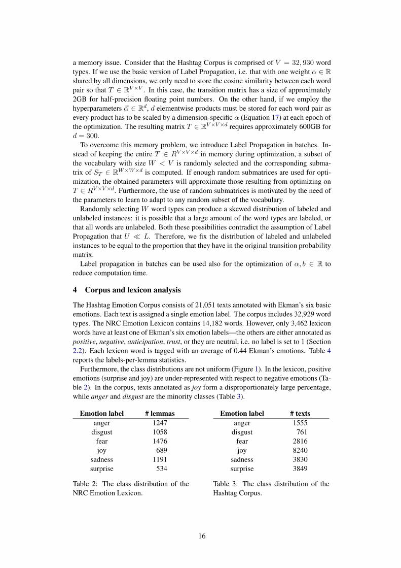
The Hashtag Emotion Corpus consists of 21,051 texts annotated with Ekman’s six basicemotions. Each text is assigned a single emotion label. The corpus includes 32,929 wordtypes. The NRC Emotion Lexicon contains 14,182 words. However, only 3,462 lexiconwords have at least one of Ekman’s six emotion labels—the others are either annotated aspositive, negative, anticipation, trust, or they are neutral, i.e. no label is set to 1 (Section2.2). Each lexicon word is tagged with an average of 0.44 Ekman’s emotions. Table 4reports the labels-per-lemma statistics.

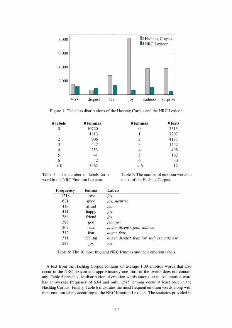
Furthermore, the class distributions are not uniform (Figure 1). In the lexicon, positiveemotions (surprise and joy) are under-represented with respect to negative emotions (Ta-ble 2). In the corpus, texts annotated as joy form a disproportionately large percentage,while anger and disgust are the minority classes (Table 3).

Emotion label # lemmasanger 1247

disgust 1058fear 1476joy 689

sadness 1191surprise 534

Table 2: The class distribution of theNRC Emotion Lexicon.

Emotion label # textsanger 1555

disgust 761fear 2816joy 8240

sadness 3830surprise 3849

Table 3: The class distribution of theHashtag Corpus.

16

anger disgust fear joy sadness surprise

2,000

4,000

6,000

8,000 Hashtag CorpusNRC Lexicon

Figure 1: The class distributions of the Hashtag Corpus and the NRC Lexicon.

# labels # lemmas0 107201 18132 9063 4474 2535 416 2> 0 3462

Table 4: The number of labels for aword in the NRC Emotion Lexicon.

# lemmas # texts0 75131 72072 41873 14424 4985 1626 30> 6 12

Table 5: The number of emotion words ina text of the Hashtag Corpus.

Frequency lemma Labels1218 love joy621 good joy, surprise418 afraid fear411 happy joy389 friend joy388 god fear, joy367 hate anger, disgust, fear, sadness342 fear anger, fear311 feeling anger, disgust, fear, joy, sadness, surprise287 joy joy

Table 6: The 10 most frequent NRC lemmas and their emotion labels.

A text from the Hashtag Corpus contains on average 1.09 emotion words that alsooccur in the NRC lexicon and approximately one third of the tweets does not containany. Table 5 presents the distribution of emotion words among texts. An emotion wordhas an average frequency of 6.64 and only 1,545 lemmas occur at least once in theHashtag Corpus. Finally, Table 6 illustrates the most frequent emotion words along withtheir emotion labels according to the NRC Emotion Lexicon. The statistics provided in

17

this paragraph were obtained by lemmatizing the Hashtag Corpus (the values resultingfrom the non-lemmatized corpus do not significantly vary).

The presented statistics clearly show that the coverage of an unexpanded lexicon is tosmall for emotion classification.

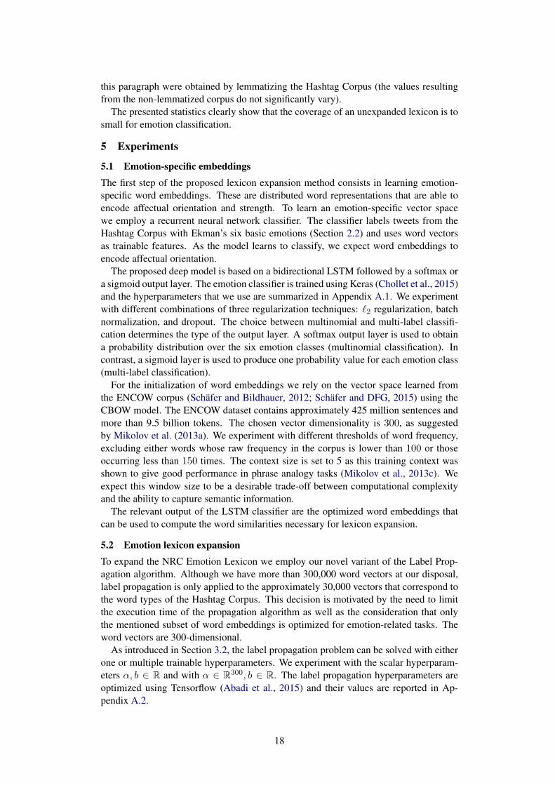
5 Experiments

5.1 Emotion-specific embeddingsThe first step of the proposed lexicon expansion method consists in learning emotion-specific word embeddings. These are distributed word representations that are able toencode affectual orientation and strength. To learn an emotion-specific vector spacewe employ a recurrent neural network classifier. The classifier labels tweets from theHashtag Corpus with Ekman’s six basic emotions (Section 2.2) and uses word vectorsas trainable features. As the model learns to classify, we expect word embeddings toencode affectual orientation.

The proposed deep model is based on a bidirectional LSTM followed by a softmax ora sigmoid output layer. The emotion classifier is trained using Keras (Chollet et al., 2015)and the hyperparameters that we use are summarized in Appendix A.1. We experimentwith different combinations of three regularization techniques: `2 regularization, batchnormalization, and dropout. The choice between multinomial and multi-label classifi-cation determines the type of the output layer. A softmax output layer is used to obtaina probability distribution over the six emotion classes (multinomial classification). Incontrast, a sigmoid layer is used to produce one probability value for each emotion class(multi-label classification).

For the initialization of word embeddings we rely on the vector space learned fromthe ENCOW corpus (Schafer and Bildhauer, 2012; Schafer and DFG, 2015) using theCBOW model. The ENCOW dataset contains approximately 425 million sentences andmore than 9.5 billion tokens. The chosen vector dimensionality is 300, as suggestedby Mikolov et al. (2013a). We experiment with different thresholds of word frequency,excluding either words whose raw frequency in the corpus is lower than 100 or thoseoccurring less than 150 times. The context size is set to 5 as this training context wasshown to give good performance in phrase analogy tasks (Mikolov et al., 2013c). Weexpect this window size to be a desirable trade-off between computational complexityand the ability to capture semantic information.

The relevant output of the LSTM classifier are the optimized word embeddings thatcan be used to compute the word similarities necessary for lexicon expansion.

5.2 Emotion lexicon expansionTo expand the NRC Emotion Lexicon we employ our novel variant of the Label Prop-agation algorithm. Although we have more than 300,000 word vectors at our disposal,label propagation is only applied to the approximately 30,000 vectors that correspond tothe word types of the Hashtag Corpus. This decision is motivated by the need to limitthe execution time of the propagation algorithm as well as the consideration that onlythe mentioned subset of word embeddings is optimized for emotion-related tasks. Theword vectors are 300-dimensional.

As introduced in Section 3.2, the label propagation problem can be solved with eitherone or multiple trainable hyperparameters. We experiment with the scalar hyperparam-eters α, b ∈ R and with α ∈ R300, b ∈ R. The label propagation hyperparameters areoptimized using Tensorflow (Abadi et al., 2015) and their values are reported in Ap-pendix A.2.

18

Furthermore, a batch-based variant of label propagation is introduced to overcomeissues of excessive time and memory needs of hyperparameter optimization. Essentially,we try to approximate the results of standard label propagation optimization—wherethe word similarity graph is comprised of all available word types—with multiple batchoptimizations—where only a subset of the word types is used to construct the similaritygraph. We expect the parameters to learn to robustly adapt to any random subset of thevocabulary and, as a consequence, to discard irrelevant features.

5.3 Emotion classification

To test our hypothesis that a combination of corpus- and lexicon-based approaches im-proves classification, we use the expanded emotion lexicon to inform the classifier andto augment the word embeddings.

Our emotion classifier is the same as the one proposed for learning task-specific wordembeddings. An embedding layer maps words to their vector representations. The em-beddings are fed to a bidirectional LSTM, followed by a softmax or a sigmoid outputlayer, for multinomial and multi-label classification respectively. Again we experimentwith `2 regularization, batch normalization, and dropout. The classifier is trained usingKeras and its hyperparameters are reported in Appendix A.3.

For the initialization of word embeddings we leverage the vector space previouslylearned by our recurrent neural network model (Section 5.1). This 300-dimensionalvector space includes approximately 30,000 word embeddings. This is the corpus-basedportion of the information we provide to the classifier.

To feed the classifier with lexicon-based information, we append the label probabilitydistribution vector of a word occurring in the expanded emotion lexicon to the corre-sponding pretrained word vector. As the lexicon is expanded to all the word types inthe Hashtag Corpus, each embedding receives an emotion-specific initialization. Noticethat the label distributions of the original lexicon words are left unvaried, due to theproperties of Label Propagation.

6 Evaluation and results

6.1 Emotion-specific embeddings

Evaluating the quality of the task-specific embeddings obtained via optimization of ouremotion classifier is not a straightforward task. One could compute sample similaritiesbetween words to see if the embeddings capture our intuition about which words shouldbe close to one another in the specialized vector space. Nevertheless, with the exceptionof very few indisputable cases, it is unfair to expect the embeddings to adhere to ourjudgments on the affective orientation of words if only because such judgments are in-herently subjective. Consider, as an example, that it might feel natural to postulate a lowsimilarity for happy and sad or a high similarity for scared and terrified. By doing so,however, we would implicitly reduce the dimensionality of the affective space to joy /sadness, or fear respectively—in terms of Ekman’s six basic emotions. Further consideran informal expression such as wtf, which repeatedly occurs in the Hashtag Corpus. It isunclear what position it should occupy in a multidimensional affective space.

As we embed the optimization of specialized embeddings in a classification task, wedecide to use the performance of the classifier as an extrinsic evaluation metric. A secondcriterion is the performance of lexicon expansion, that we evaluate using 10-fold cross-validation. The results of these evaluations are presented in the next two subsections.

19

6.2 Emotion lexicon expansionTo perform an intrinsic evaluation of our lexicon expansion method, we choose 10-foldcross-validation. The intersection between the word types of the Hashtag Corpus and theNRC Emotion Lexicon is partitioned into 10 equal sized subsamples. Cross-validationis repeated 10 times and each of the subsamples is used once as validation data.

The quality of the expanded lexicon is assessed by computing the average Kullback-Leibler divergence between the emotion label probability distributions obtained normal-izing the NRC Emotion Lexicon and the the distributions resulting from label propaga-tion.

Three baseline lexicon expansion methods are introduced: (i) assigning a uniformclass distribution to all words, (ii) assigning to all words a distribution where all theprobability mass is given to the majority class based on the Hashtag Corpus, (iii) assign-ing to all words the prior class distribution of the Hashtag Corpus.

Table 7 shows the average Kullback–Leibler divergence for 10-fold cross-validationof the described lexicon expansion techniques.

Lexicon expansion KL divergenceUniform distribution 1.34Majority class (Hashtag Corpus) 21.32Prior class distribution (Hashtag Corpus) 1.53Label propagation (α ∈ R) 1.31Batch label propagation (α ∈ R) 1.31

Table 7: Average Kullback–Leibler divergence for 10-fold cross-validation on the NRCEmotion Lexicon. The lowest divergence is obtained using label propagation.

Interestingly, the uniform class distribution yields an even lower divergence than theprior class distribution of the Hashtag Corpus. Although its low divergence, the uniformdistribution clearly cannot be used in practice as it is, by definition, uninformative.

Label propagation with a scalar parameter α is the method that best minimizes theaverage Kullback–Leibler divergence, indicating that the quality of the expanded lexi-con is satisfactory. Remarkably, batch label propagation performs similarly to standardpropagation although it uses batches of size 5,000 (compared to a total of more than30,000 word types). This result shows that batch approximation can work for graphpropagation, at least when the number of trainable parameters is limited.

In contrast, using batch approximation to optimize the parameter vector ~α appears torequire either a large batch size, or a large number of training batches, both of whichdemand a long runtime. Optimization performed with 500 batches of size 3,000 (eachbatch is trained on for 5 epochs) yields an average Kullback–Leibler divergence of 14.37.Increasing the batch size to 4,000 and the number of batches to 1,500 (each batch istrained on for 3 epochs), the average Kullback–Leibler divergence drops to 13.23. Wecan therefore conclude that a parameter vector ~α is ineffective if is optimized using batchgradient descent. It remains unclear if ~α is generally inadequate for this task or if itsoptimization requires the entire dataset. Therefore, we will only report the classificationresults based on label propagation with a scalar parameter α.

6.3 Emotion classificationTo evaluate the proposed emotion classifier, we introduce multiple baselines. The lowerbound is represented by a random classifier. Then we implemented a trivial count-basedclassifier that assigns emotion labels based on the NRC Emotion Lexicon. In particular,

20

this trivial classifier counts the lexicon words occurring in a paragraph for each emotionclass—fr (ek)—, and produces a label probability distribution over m classes:

P (ei) =fr (ei)∑m

k=1 fr (ek)

A more competitive baseline is represented by a version of the LSTM classifier in-troduced at the beginning of this section that only exploits our emotion-specific wordembeddings. As a final alternative, the pretrained emotion-specific embeddings are con-catenated with the probability distributions indicated by the unexpanded NRC EmotionLexicon. Words that do not occur in the lexicon have their vectors concatenated with avector of probabilities randomly sampled from a uniform distribution. Uniform initial-ization outperforms the overall probability distribution of emotions in the lexicon.

The precision, accuracy, and F1 score of all the presented classifiers are reported inTables 8 and 9. All metrics are computed using micro-averaging to allow a comparisonwith previous work and to reduce the effect of label imbalance. Using macro-averagingwould assign more weight to the majority classes, for which classifiers tend to performbetter due to the larger amount of training instances.

Classifier P R F1Random 16.9 16.9 16.9Count-based (NRC Emotion Lexicon) 15.7 15.7 15.7One-vs-all SVM (Mohammad and Kiritchenko, 2015) 55.1 45.6 49.9Multinomial LSTM 55.0 55.0 55.0Multinomial LSTM + NRC Emotion Lexicon 55.2 55.2 55.2Multinomial LSTM + expanded lexicon (α ∈ R) 56.2 56.2 56.2Students 40.9 40.4 40.6

Table 8: Results of classification on the Hashtag Emotion Corpus. Although the bidirec-tional LSTM classifier represents a strong baseline, using the expanded lexicon boostsclassification accuracy.

For the Hashtag Emotion Corpus, the bidirectional LSTM classifier introduced asa baseline outperforms one-vs-all SVM with binary features, setting a relatively highlower bound to our task. Including the label distributions of the NRC Emotion Lexiconas features slightly increases the classifier accuracy, already indicating that corpus-basedand lexicon-based information is complementary. The limited increment in accuracy canbe explained by the fact that a text from the Hashtag Corpus includes on average 1.09NRC emotion words and that approximately one third of the tweets does not containany NRC lemmas. The LSTM classifier shows a remarkable increase in accuracy whenthe expanded lexicon is provided. Although we can assume that quality of the expandedlexicon is lower than the quality of the hand-annotated NRC Emotion Lexicon, the widercoverage of the former seems to successfully help the classifier.

Regardless of whether the LSTM classifier uses no lexicon, the NRC lexicon, or theexpanded one, the multinomial variant consistently obtains a higher accuracy. The clas-sification report of our best classifier is presented in Table 11.

The fact that label propagation is performed on ENCOW embeddings with backprop-agation from the supervised learning task possibly suggests that the expanded lexiconis tailored to the training dataset (Hashtag Corpus). However, the performance of theLSTM classifier is boosted by the expanded lexicon even on a dataset from a differentdomain (SemEval headlines). This result seems to imply that the Hashtag Corpus is a

21

Classifier P R F1One-vs-all SVM (Mohammad and Kiritchenko, 2015)

1. ngrams in headlines dataset and Hashtag Corpus + domain adaptation 46.0 35.5 40.12. ngrams in headlines dataset + NRC Emotion Lexicon 46.7 38.6 42.2

Multi-label LSTM 38.8 50.3 43.8Multi-label LSTM + NRC Emotion Lexicon 39.2 50.9 44.3Multi-label LSTM + expanded lexicon 43.1 48.9 45.9

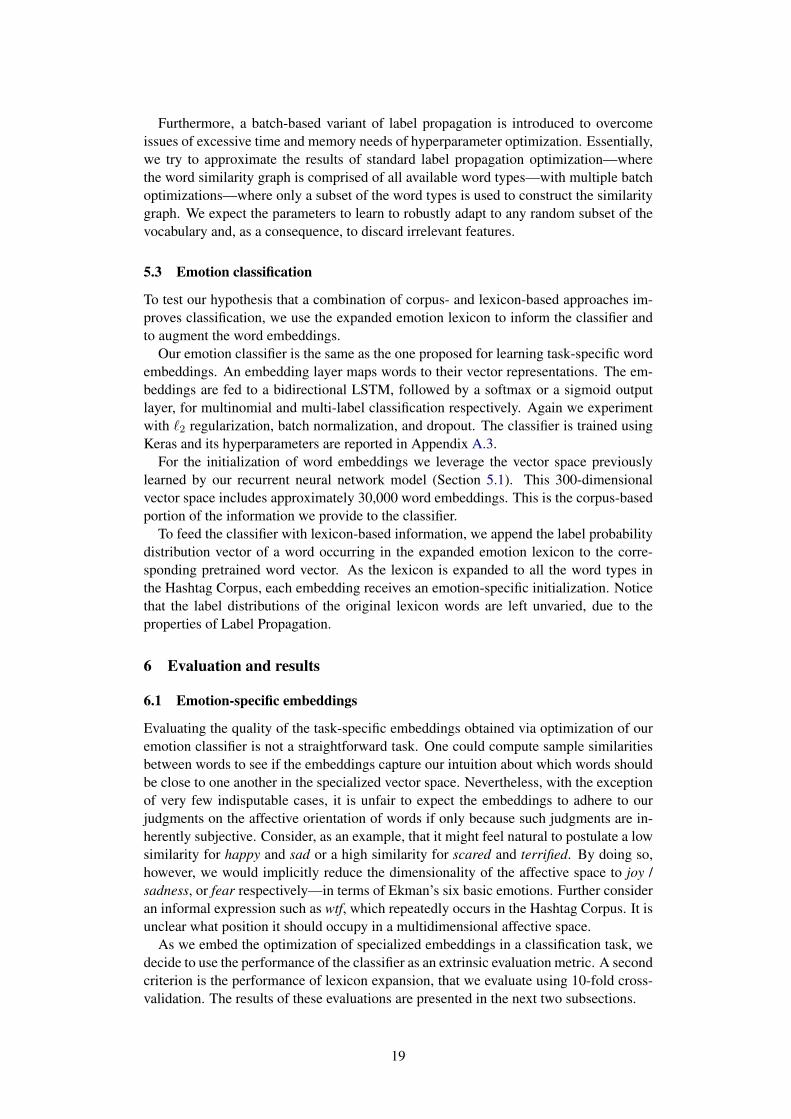
Table 9: Results of classification on the SemEval headlines dataset. The most accurateclassifier is the bidirectional LSTM informed with the expanded lexicon.

sufficiently large resource, which grants coverage over a wide variety of word types andencodes context-independent information.

Humans as classifiersIn Section 2.1, we have reported the inter-annotator agreement studies conducted byStrapparava and Mihalcea (2007) for the SemEval headlines corpus. These have shownthat trained annotators agree with a Pearson correlation of 53.67 using the simple averageover classes, and r = 43 using the frequency-based average.

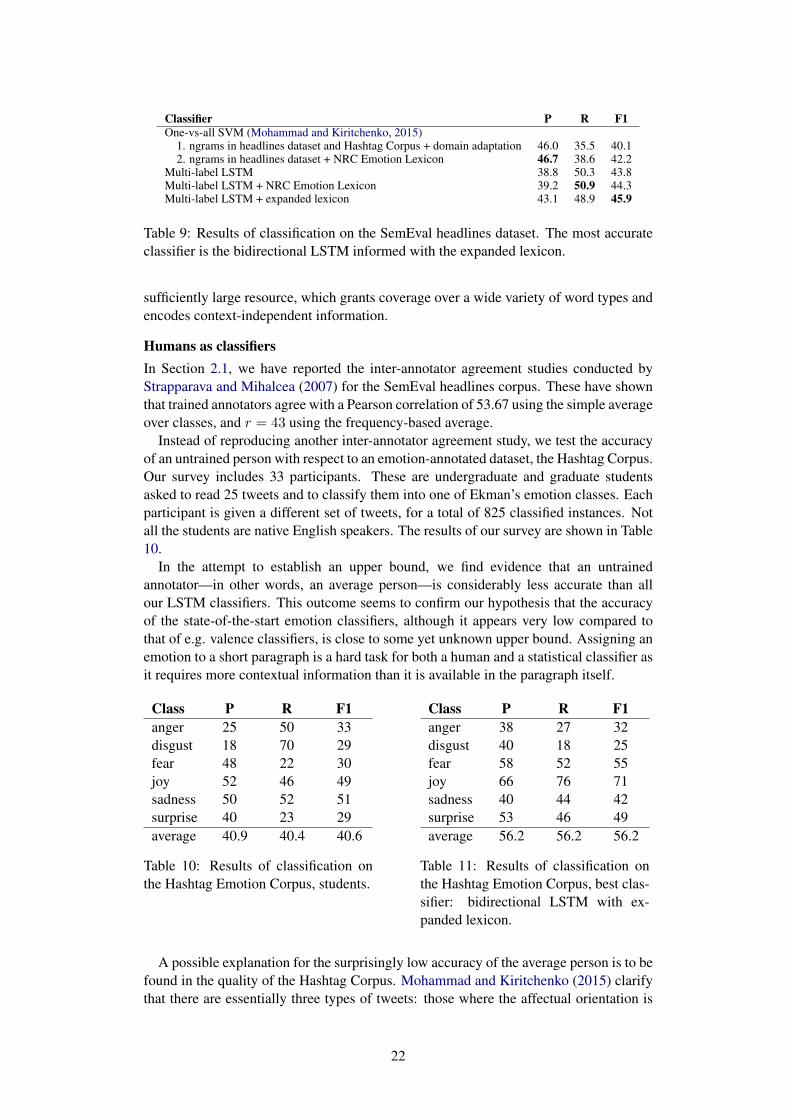
Instead of reproducing another inter-annotator agreement study, we test the accuracyof an untrained person with respect to an emotion-annotated dataset, the Hashtag Corpus.Our survey includes 33 participants. These are undergraduate and graduate studentsasked to read 25 tweets and to classify them into one of Ekman’s emotion classes. Eachparticipant is given a different set of tweets, for a total of 825 classified instances. Notall the students are native English speakers. The results of our survey are shown in Table10.

In the attempt to establish an upper bound, we find evidence that an untrainedannotator—in other words, an average person—is considerably less accurate than allour LSTM classifiers. This outcome seems to confirm our hypothesis that the accuracyof the state-of-the-start emotion classifiers, although it appears very low compared tothat of e.g. valence classifiers, is close to some yet unknown upper bound. Assigning anemotion to a short paragraph is a hard task for both a human and a statistical classifier asit requires more contextual information than it is available in the paragraph itself.

Class P R F1anger 25 50 33disgust 18 70 29fear 48 22 30joy 52 46 49sadness 50 52 51surprise 40 23 29average 40.9 40.4 40.6

Table 10: Results of classification onthe Hashtag Emotion Corpus, students.

Class P R F1anger 38 27 32disgust 40 18 25fear 58 52 55joy 66 76 71sadness 40 44 42surprise 53 46 49average 56.2 56.2 56.2

Table 11: Results of classification onthe Hashtag Emotion Corpus, best clas-sifier: bidirectional LSTM with ex-panded lexicon.

A possible explanation for the surprisingly low accuracy of the average person is to befound in the quality of the Hashtag Corpus. Mohammad and Kiritchenko (2015) clarifythat there are essentially three types of tweets: those where the affectual orientation is

22

anger disgust fear joy sadness surprise

10

20

30

40 Hashtag CorpusSurvey

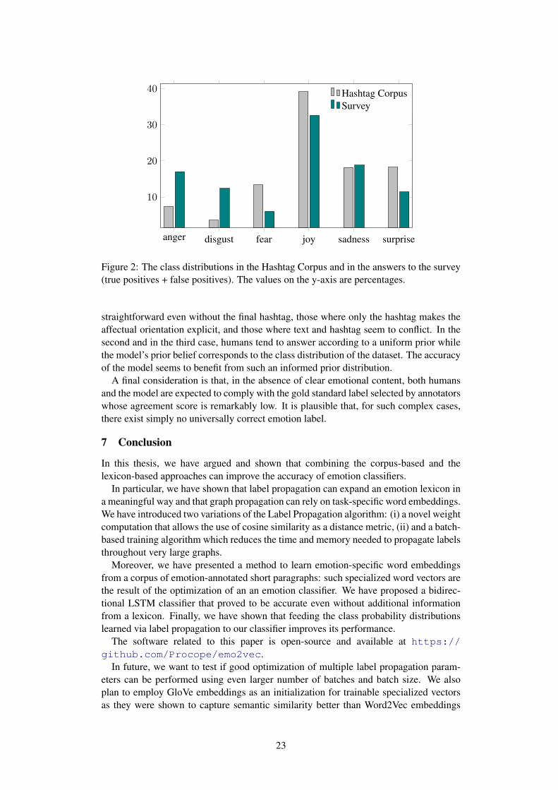
Figure 2: The class distributions in the Hashtag Corpus and in the answers to the survey(true positives + false positives). The values on the y-axis are percentages.

straightforward even without the final hashtag, those where only the hashtag makes theaffectual orientation explicit, and those where text and hashtag seem to conflict. In thesecond and in the third case, humans tend to answer according to a uniform prior whilethe model’s prior belief corresponds to the class distribution of the dataset. The accuracyof the model seems to benefit from such an informed prior distribution.

A final consideration is that, in the absence of clear emotional content, both humansand the model are expected to comply with the gold standard label selected by annotatorswhose agreement score is remarkably low. It is plausible that, for such complex cases,there exist simply no universally correct emotion label.

7 Conclusion

In this thesis, we have argued and shown that combining the corpus-based and thelexicon-based approaches can improve the accuracy of emotion classifiers.

In particular, we have shown that label propagation can expand an emotion lexicon ina meaningful way and that graph propagation can rely on task-specific word embeddings.We have introduced two variations of the Label Propagation algorithm: (i) a novel weightcomputation that allows the use of cosine similarity as a distance metric, (ii) and a batch-based training algorithm which reduces the time and memory needed to propagate labelsthroughout very large graphs.

Moreover, we have presented a method to learn emotion-specific word embeddingsfrom a corpus of emotion-annotated short paragraphs: such specialized word vectors arethe result of the optimization of an an emotion classifier. We have proposed a bidirec-tional LSTM classifier that proved to be accurate even without additional informationfrom a lexicon. Finally, we have shown that feeding the class probability distributionslearned via label propagation to our classifier improves its performance.

The software related to this paper is open-source and available at https://github.com/Procope/emo2vec.

In future, we want to test if good optimization of multiple label propagation param-eters can be performed using even larger number of batches and batch size. We alsoplan to employ GloVe embeddings as an initialization for trainable specialized vectorsas they were shown to capture semantic similarity better than Word2Vec embeddings

23

(Pennington et al., 2014). Furthermore, we want to introduce lexical-contrast informa-tion into our task-specialization routine using wordnets, and to—instead of optimizingword embeddings singularly—learn a rotation that can transform the entire vector spaceinto a task-specific one.

Emotion-specific embeddings have proven to be a reliable source for the constructionof similarity graphs but there may be other interesting options: we will experiment withco-occurrence counts and with wordnets in order to discover alternative meaningful wordrepresentations.

24

ReferencesMartın Abadi, Ashish Agarwal, Paul Barham, Eugene Brevdo, Zhifeng Chen, Craig Citro,

Greg S. Corrado, Andy Davis, Jeffrey Dean, Matthieu Devin, Sanjay Ghemawat, Ian Goodfel-low, Andrew Harp, Geoffrey Irving, Michael Isard, Yangqing Jia, Rafal Jozefowicz, LukaszKaiser, Manjunath Kudlur, Josh Levenberg, Dan Mane, Rajat Monga, Sherry Moore, DerekMurray, Chris Olah, Mike Schuster, Jonathon Shlens, Benoit Steiner, Ilya Sutskever, KunalTalwar, Paul Tucker, Vincent Vanhoucke, Vijay Vasudevan, Fernanda Viegas, Oriol Vinyals,Pete Warden, Martin Wattenberg, Martin Wicke, Yuan Yu, and Xiaoqiang Zheng. 2015. Ten-sorFlow: Large-scale machine learning on heterogeneous systems. Software available fromtensorflow.org. http://tensorflow.org/.

Cecilia Ovesdotter Alm, Dan Roth, and Richard Sproat. 2005. Emotions from text: machinelearning for text-based emotion prediction. In Proceedings of the conference on human lan-guage technology and empirical methods in natural language processing. Association forComputational Linguistics, pages 579–586.

Saima Aman and Stan Szpakowicz. 2007. Identifying expressions of emotion in text. In Inter-national Conference on Text, Speech and Dialogue. Springer, pages 196–205.

Alina Andreevskaia and Sabine Bergler. 2008. When specialists and generalists work together:Overcoming domain dependence in sentiment tagging. In ACL. pages 290–298.

Yoshua Bengio, Patrice Simard, and Paolo Frasconi. 1994. Learning long-term dependencieswith gradient descent is difficult. IEEE transactions on neural networks 5(2):157–166.

Felipe Bravo-Marquez, Eibe Frank, Saif M Mohammad, and Bernhard Pfahringer. 2016. Deter-mining word–emotion associations from tweets by multi-label classification. In WI’16. IEEEComputer Society, pages 536–539.

Soumaya Chaffar and Diana Inkpen. 2011. Using a heterogeneous dataset for emotion analysisin text. In Canadian Conference on Artificial Intelligence. Springer, pages 62–67.

Francois Chollet et al. 2015. Keras. https://github.com/fchollet/keras.

Ronan Collobert, Jason Weston, Leon Bottou, Michael Karlen, Koray Kavukcuoglu, and PavelKuksa. 2011. Natural language processing (almost) from scratch. Journal of Machine Learn-ing Research 12(Aug):2493–2537.

Paul Ekman. 1992. An argument for basic emotions. Cognition & emotion 6(3-4):169–200.

Jeffrey L Elman. 1990. Finding structure in time. Cognitive science 14(2):179–211.

Andrea Esuli and Fabrizio Sebastiani. 2007. Sentiwordnet: A high-coverage lexical resource foropinion mining. Evaluation pages 1–26.

Alex Graves and Jurgen Schmidhuber. 2005. Framewise phoneme classification with bidirec-tional lstm and other neural network architectures. Neural Networks 18(5):602–610.

Michael U Gutmann and Aapo Hyvarinen. 2012. Noise-contrastive estimation of unnormalizedstatistical models, with applications to natural image statistics. Journal of Machine LearningResearch 13(Feb):307–361.

Sepp Hochreiter. 1991. Untersuchungen zu dynamischen neuronalen Netzen. Ph.D. thesis,diploma thesis, institut fur informatik, lehrstuhl prof. brauer, technische universitat munchen.

Sepp Hochreiter and Jurgen Schmidhuber. 1997. Long short-term memory. Neural computation9(8):1735–1780.

Sergey Ioffe and Christian Szegedy. 2015. Batch normalization: Accelerating deep networktraining by reducing internal covariate shift. arXiv preprint arXiv:1502.03167 .

Carroll E Izard. 1971. The face of emotion. .

25

Thorsten Joachims. 1999. Transductive inference for text classification using support vectormachines. In ICML. volume 99, pages 200–209.

Alistair Kennedy and Diana Inkpen. 2006. Sentiment classification of movie reviews using con-textual valence shifters. Computational intelligence 22(2):110–125.

Joseph B Kruskal. 1956. On the shortest spanning subtree of a graph and the traveling salesmanproblem. Proceedings of the American Mathematical society 7(1):48–50.

Igor Labutov and Hod Lipson. 2013. Re-embedding words. In ACL (2). pages 489–493.

Yann A LeCun, Leon Bottou, Genevieve B Orr, and Klaus-Robert Muller. 2012. Efficient back-prop. In Neural networks: Tricks of the trade, Springer, pages 9–48.

Tomas Mikolov, Kai Chen, Greg Corrado, and Jeffrey Dean. 2013a. Efficient estimation of wordrepresentations in vector space. arXiv preprint arXiv:1301.3781 .

Tomas Mikolov, V Le Quoc, and Ilya Sutskever. 2013b. Exploiting similarities among languagesfor machine translation. arxiv.

Tomas Mikolov, Ilya Sutskever, Kai Chen, Greg S Corrado, and Jeff Dean. 2013c. Distributedrepresentations of words and phrases and their compositionality. In Advances in neural infor-mation processing systems. pages 3111–3119.

Tomas Mikolov, Wen-tau Yih, and Geoffrey Zweig. 2013d. Linguistic regularities in continuousspace word representations. In Hlt-naacl. volume 13, pages 746–751.

Saif M Mohammad. 2015. Sentiment analysis: Detecting valence, emotions, and other affectualstates from text. Emotion Measurement pages 201–238.

Saif M Mohammad and Svetlana Kiritchenko. 2015. Using hashtags to capture fine emotioncategories from tweets. Computational Intelligence 31(2):301–326.

Saif M Mohammad and Peter D Turney. 2013. Crowdsourcing a word–emotion associationlexicon. Computational Intelligence 29(3):436–465.

Alena Neviarouskaya, Helmut Prendinger, and Mitsuru Ishizuka. 2009. Compositionality prin-ciple in recognition of fine-grained emotions from text. In ICWSM.

Bo Pang, Lillian Lee, and Shivakumar Vaithyanathan. 2002. Thumbs up?: sentiment classifi-cation using machine learning techniques. In Proceedings of the ACL-02 conference on Em-pirical methods in natural language processing-Volume 10. Association for ComputationalLinguistics, pages 79–86.

Bo Pang, Lillian Lee, et al. 2008. Opinion mining and sentiment analysis. Foundations andTrends R© in Information Retrieval 2(1–2):1–135.

Jeffrey Pennington, Richard Socher, and Christopher D Manning. 2014. Glove: Global vectorsfor word representation. In EMNLP. volume 14, pages 1532–1543.

Sasa Petrovic, Miles Osborne, and Victor Lavrenko. 2010. The edinburgh twitter corpus. InProceedings of the NAACL HLT 2010 Workshop on Computational Linguistics in a World ofSocial Media. pages 25–26.

Robert Plutchik. 1980. A general psychoevolutionary theory of emotion. Theories of emotion1(3-31):4.

Guang Qiu, Bing Liu, Jiajun Bu, and Chun Chen. 2009. Expanding domain sentiment lexiconthrough double propagation. In IJCAI. volume 9, pages 1199–1204.

David E Rumelhart, Geoffrey E Hinton, and Ronald J Williams. 1988. Learning representationsby back-propagating errors. Cognitive modeling 5(3):1.

Roland Schafer and Felix Bildhauer. 2012. Building large corpora from the web using a newefficient tool chain. In LREC. pages 486–493.

26

Roland Schafer and Linguistic Web Characterization DFG. 2015. Processing and querying largeweb corpora with the cow14 architecture. In Proceedings of the 3rd Workshop on Challengesin the Management of Large Corpora. pages 28–34.

Klaus R Scherer and Harald G Wallbott. 1994. Evidence for universality and cultural variationof differential emotion response patterning. Journal of personality and social psychology66(2):310.

Nitish Srivastava, Geoffrey E Hinton, Alex Krizhevsky, Ilya Sutskever, and Ruslan Salakhutdi-nov. 2014. Dropout: a simple way to prevent neural networks from overfitting. Journal ofMachine Learning Research 15(1):1929–1958.

Carlo Strapparava and Rada Mihalcea. 2007. Semeval-2007 task 14: Affective text. In Proceed-ings of the 4th International Workshop on Semantic Evaluations. Association for Computa-tional Linguistics, pages 70–74.

Carlo Strapparava and Rada Mihalcea. 2008. Learning to identify emotions in text. In Proceed-ings of the 2008 ACM symposium on Applied computing. ACM, pages 1556–1560.

Carlo Strapparava, Alessandro Valitutti, and Oliviero Stock. 2006. The affective weight of lex-icon. In Proceedings of the fifth international conference on language resources and evalua-tion. pages 423–426.

Carlo Strapparava, Alessandro Valitutti, et al. 2004. Wordnet affect: an affective extension ofwordnet. In LREC. Citeseer, volume 4, pages 1083–1086.

Maite Taboada, Julian Brooke, Milan Tofiloski, Kimberly Voll, and Manfred Stede. 2011.Lexicon-based methods for sentiment analysis. Computational linguistics 37(2):267–307.

Duyu Tang, Furu Wei, Nan Yang, Ming Zhou, Ting Liu, and Bing Qin. 2014. Learningsentiment-specific word embedding for twitter sentiment classification. In ACL (1). pages1555–1565.

Peter D Turney. 2002. Thumbs up or thumbs down?: semantic orientation applied to unsuper-vised classification of reviews. In Proceedings of the 40th annual meeting on association forcomputational linguistics. Association for Computational Linguistics, pages 417–424.

Peter D Turney. 2012. Domain and function: A dual-space model of semantic relations andcompositions. Journal of Artificial Intelligence Research 44:533–585.

Vladimir Naumovich Vapnik and Vlamimir Vapnik. 1998. Statistical learning theory, volume 1.Wiley New York.

Paul J Werbos. 1990. Backpropagation through time: what it does and how to do it. Proceedingsof the IEEE 78(10):1550–1560.

Min Yang, Wenting Tu, Ziyu Lu, Wenpeng Yin, and Kam-Pui Chow. 2015. Lcct: a semisuper-vised model for sentiment classification. In Human Language Technologies: The 2015 AnnualConference of the North American Chapter of the ACL. Association for Computational Lin-guistics (ACL).

Zhixin Zhou, Xiuzhen Zhang, and Mark Sanderson. 2014. Sentiment analysis on twitter throughtopic-based lexicon expansion. In Australasian Database Conference. Springer, pages 98–109.

Xiaojin Zhu and Zoubin Ghahramani. 2002. Learning from labeled and unlabeled data with labelpropagation .

27

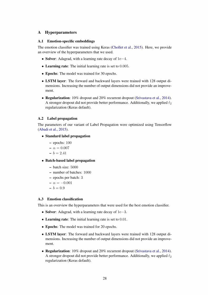
A Hyperparameters

A.1 Emotion-specific embeddingsThe emotion classifier was trained using Keras (Chollet et al., 2015). Here, we providean overview of the hyperparameters that we used.

• Solver: Adagrad, with a learning rate decay of 1e−4.

• Learning rate: The initial learning rate is set to 0.005.

• Epochs: The model was trained for 30 epochs.

• LSTM layer: The forward and backward layers were trained with 128 output di-mensions. Increasing the number of output dimensions did not provide an improve-ment.

• Regularization: 10% dropout and 20% recurrent dropout (Srivastava et al., 2014).A stronger dropout did not provide better performance. Additionally, we applied `2regularization (Keras default).

A.2 Label propagationThe parameters of our variant of Label Propagation were optimized using Tensorflow(Abadi et al., 2015).

• Standard label propagation

– epochs: 100

– α = 0.007

– b = 2.41

• Batch-based label propagation

– batch size: 5000

– number of batches: 1000

– epochs per batch: 3

– α = −0.001

– b = 0.9

A.3 Emotion classificationThis is an overview the hyperparameters that were used for the best emotion classifier.

• Solver: Adagrad, with a learning rate decay of 1e−3.

• Learning rate: The initial learning rate is set to 0.01.

• Epochs: The model was trained for 20 epochs.

• LSTM layer: The forward and backward layers were trained with 128 output di-mensions. Increasing the number of output dimensions did not provide an improve-ment.

• Regularization: 10% dropout and 20% recurrent dropout (Srivastava et al., 2014).A stronger dropout did not provide better performance. Additionally, we applied `2regularization (Keras default).

28