Semi-Online Bipartite MatchingRavi KumarGoogle, Mountain View, CA, USAravi.k53@gmail.com

Manish PurohitGoogle, Mountain View, CA, USAmpurohit@google.com

Aaron SchildUniversity of California, Berkeley, CA, USAaschild@berkeley.edu

Zoya SvitkinaGoogle, Mountain View, CA, USAzoya@cs.cornell.edu

Erik VeeGoogle, Mountain View, CA, USAerikvee@google.com

AbstractIn this paper we introduce the semi-online model that generalizes the classical online computa-tional model. The semi-online model postulates that the unknown future has a predictable partand an adversarial part; these parts can be arbitrarily interleaved. An algorithm in this modeloperates as in the standard online model, i.e., makes an irrevocable decision at each step.

We consider bipartite matching in the semi-online model. Our main contributions are com-petitive algorithms for this problem and a near-matching hardness bound. The competitive ratioof the algorithms nicely interpolates between the truly offline setting (i.e., no adversarial part)and the truly online setting (i.e., no predictable part).

2012 ACM Subject Classification Theory of computation → Online algorithms

Keywords and phrases Semi-Online Algorithms, Bipartite Matching

Digital Object Identifier 10.4230/LIPIcs.ITCS.2019.50

Related Version A full version of the paper is available at https://arxiv.org/abs/1812.00134.

Acknowledgements We thank Michael Kapralov for introducing us to the bipartite matchingskeleton decomposition in [7].

1 Introduction

Modeling future uncertainty in data while ensuring that the model remains both realisticand tractable has been a formidable challenge facing the algorithms research community.One of the more popular, and reasonably realistic, such models is the online computationalmodel. In its classical formulation, data arrives one at a time and upon each arrival, thealgorithm has to make an irrevocable decision agnostic of future arrivals. Online algorithmsboast a rich literature and problems such as caching, scheduling and matching, each of which

© Ravi Kumar, Manish Purohit, Aaron Schild, Zoya Svitkina, and Erik Vee;licensed under Creative Commons License CC-BY

10th Innovations in Theoretical Computer Science (ITCS 2019).Editor: Avrim Blum; Article No. 50; pp. 50:1–50:20

Leibniz International Proceedings in InformaticsSchloss Dagstuhl – Leibniz-Zentrum für Informatik, Dagstuhl Publishing, Germany

50:2 Semi-Online Bipartite Matching

abstracts common practical scenarios, have been extensively investigated [4, 20]. Competitiveanalysis, which measures how well an online algorithm performs compared to the best offlinealgorithm that knows the future, has been a linchpin in the study of online algorithms.

While online algorithms capture some aspect of the future uncertainty in the data, thenotion of competitive ratio is inherently worst-case and hence the quantitative guarantees itoffers are often needlessly pessimistic. A natural question that then arises is : how can weavoid modeling the worst-case scenario in online algorithms? Is there a principled way toincorporate some knowledge we have about the future? There have been a few efforts tryingto address this point from different angles. One line of attack has been to consider oracles thatoffer some advice on the future; such oracles, for instance, could be based on machine-learningmethods. This model has been recently used to improve the performance of online algorithmsfor reserve price optimization, caching, ski-rental, and scheduling [19, 16, 14]. Another line ofattack posits a distribution on the data [5, 17, 21] or the arrival model; for instance, randomarrival models have been popular in online bipartite matching and are known to beat theworst-case bounds [10, 18]. A different approach is to assume a distribution on future inputs;the field of stochastic online optimization focuses on this setting [8]. The advice complexitymodel, where the partial information about the future is quantified as advice bits to anonline algorithm, has been studied as well in complexity theory [3].

In this work we take a different route. At a very high level, the idea is to tease the futuredata apart into a predictable subset and the remaining adversarial subset. As the namesconnote, the algorithm can be assumed to know everything about the former but nothingabout the latter. Furthermore, the predictable and adversarial subsets can arrive arbitrarilyinterleaved yet the algorithm still has to operate as in the classical online model, i.e., makeirrevocable decisions upon each arrival. Our model thus offers a natural interpolationbetween the traditional offline and online models; we call ours the semi-online model. Ourgoal is to study algorithms in the semi-online model and to analyze their competitiveratios; unsurprisingly, the bounds depend on the size of the adversarial subset. Ideally, thecompetitive ratio should approach the offline optimum bounds if the adversarial fractionis vanishing and should approach the online optimum bounds if the predictable fraction isvanishing.

Bipartite matching. As a concrete problem in the semi-online setting, we focus on bipartitematching. In the well-known online version of the problem, which is motivated by onlineadvertising, there is a bipartite graph with an offline side that is known in advance andan online side that is revealed one node at a time together with its incident edges. In thesemi-online model, the nodes in the online side are partitioned into a predicted set of sizen − d and an adversarial set of size d. The algorithm knows the incident edges of all thenodes in the former but nothing about the nodes in the latter. We can thus also interpretthe setting as online matching with partial information and predictable uncertainty (pardonthe oxymoron). In online advertising applications, there are many predictably unpredictableevents. For example, during the soccer world cup games, we know the nature of web trafficwill be unpredictable but nothing more, since the actual characteristics will depend on howthe game progresses and which team wins.

We also consider a variant of semi-online matching in which the algorithm does not knowwhich nodes are predictable and which are adversarial. In other words, the algorithm receivesa prediction for all online nodes, but the predictions are correct only for some n− d of them.We call this the agnostic case.

R. Kumar, M. Purohit, A. Schild, Z. Svitkina, and E. Vee 50:3

Main results. In this paper, we assume that the optimum solution on the bipartite graph,formed by the offline nodes on one side and by the predicted and adversarial nodes on theother, is a perfect matching1. We present two algorithms and a hardness result for thesemi-online bipartite matching problem. Let δ = d/n be the fraction of adversarial nodes.The Iterative Sampling algorithm, described in Section 3, obtains a competitive ratio of(1 − δ + δ2

2 (1 − 1/e))2. This algorithm “reserves” a set of offline nodes to be matched tothe adversarial nodes by repeatedly selecting a random offline node that is unnecessary formatching the predictable nodes. It is easy to see that algorithms that deterministicallyreserve a set of offline nodes can easily be thwarted by the adversary.

The second algorithm, described in Section 4, achieves an improved competitive ratioof (1 − δ + δ2(1 − 1/e)). This algorithm samples a maximum matching in the predictedgraph by first finding a matching skeleton [7, 15] and then sampling a matching from eachcomponent in the skeleton using the dependent rounding scheme of [6]. This allows us tosample a set of offline nodes that, in expectation, has a large overlap with the set matchedto adversarial nodes in the optimal solution. Surprisingly, in Section 5, we show that it ispossible to sample from arbitrary set systems so that the same “large overlap” property ismaintained. We prove the existence of such distributions using LP duality and believe thatthis result may be of independent interest.

To complement the algorithms, in Section 6 we obtain a hardness result showing thatthe above competitive ratios are near-optimal. In particular, no randomized algorithm canachieve a competitive ratio better than (1 − δe−δ) ≈ (1 − δ + δ2 − δ3/2 + . . .). Note thatthis expression coincides with the best offline bound (i.e, 1) and the best online bound (i.e.,1 − 1/e) at the extremes of δ = 0 and δ = 1, respectively. We conjecture this to be theoptimal bound for the problem.

Extensions. In Section 7, we explore variants of the semi-online matching model, includingthe agnostic version and fractional matchings, and present upper and lower bounds in thosesettings. To illustrate the generality of our semi-online model, we consider a semi-onlineversion of the classical ski rental problem. In this version, the skier knows whether or notshe’ll ski on certain days while other days are uncertain. Interestingly, there is an algorithmwith a competitive ratio of the same form as our hardness result for matchings, namely1− (1− x)e−(1−x), where (1− x) is a parameter analogous to δ in the matching problem.We wonder if this form plays a role in semi-online algorithms similar to what (1− 1/e) hasin many online algorithms [11].

Other related work. The use of (machine learned) predictions for revenue optimizationproblems was first proposed in [19]. The concepts were formalized further and applied toonline caching in [16] and ski rental and non-clairvoyant scheduling in [14]. Online matchingwith forecasts was first studied in [22]; however, that paper is on forecasting the demandsrather than the structure of the graph as in our case. The problem of online matching whenedges arrive in batches was considered in [15] where a (1/2 + 2−O(s))-competitive ratio isshown, with s the number of stages. However, the batch framework differs from ours in thatin our case, the nodes arrive one at a time and are arbitrarily interleaved.

1 Our techniques extend to the case without a perfect matching; we defer the proof of the general case tothe full version of the paper.

2 Observe that an algorithm that ignores all the adversarial nodes and outputs a maximum matching inthe predicted graph achieves a competitive ratio of only 1 − δ.

ITCS 2019

50:4 Semi-Online Bipartite Matching

There has been a lot of work on online bipartite matching and its variants. The RANKINGalgorithm [13] selects a random permutation of the offline nodes and then matches each onlinenode to its unmatched neighbor that appears earliest in the permutation. It is well-known toobtain a competitive ratio of (1− 1/e), which is best possible. For a history of the problemand significant advances, see the monograph [20]. The ski rental problem has also beenextensively studied; the optimal randomized algorithm has ratio e/(e− 1) [12]. The term“semi-online” has been used in scheduling when an online scheduler knows the sum of thejobs’ processing times (e.g., see [1]) and in online bin-packing when a lookahead of the nextfew elements is available (e.g., see [2]); our use of the term is more quantitative in nature.

2 Model

We now formally define the semi-online bipartite matching problem. We have a bipartitegraph G = (U, V,EG) where U is the set of nodes available offline and nodes in V arrive online.Further, the online set V is partitioned into the predicted nodes VP and the adversarial nodesVA. The predicted graph H = (U, VP , EH) is the subgraph of G induced on the nodes in Uand VP . Initially, an algorithm only knows H and is unaware of edges between U and VA.The algorithm is allowed to preprocess H before any online node actually arrives. In theonline phase, at each step, one node of V is revealed with its incident edges, and has to beeither irrevocably matched to some node in U or abandoned. Nodes of V are revealed in anarbitrary order3 and the process continues until all of V has been revealed.

We note that when a node v ∈ V is revealed, the algorithm can “recognize” it by itsedges, i.e., if there is some node v′ ∈ VP that has the same set of neighbors as v and has notbeen seen before, then v can be assumed to be v′. There could be multiple identical nodes inVP , but it is not important to distinguish between them. If an online node comes that is notin VP , then the algorithm can safely assume that it is from VA. (In Section 7, we consider amodel where the predicted graph can have errors and hence this assumption is invalid.)

We introduce a quantity δ to measure the level of knowledge that the algorithm has aboutthe input graph G. Competitive ratios that we obtain are functions of δ. For any graph I,let ν(I) denote the size of the maximum matching in I. Then we define δ = δ(G) = 1− ν(H)

ν(G) .Intuitively, the closer δ is to 0, the more information the predicted graph H contains andthe closer the instance is to an offline problem. Conversely, δ close to 1 indicates an instanceclose to the pure online setting. Note that the algorithm does not necessarily know δ, butwe use it in the analysis to bound the competitive ratio. For convenience, in this paperwe assume that the input graph G contains a perfect matching. Let n = |U | = |V | be thenumber of nodes on each side and d = |VA| be the number of adversarial online nodes. In thiscase, δ simplifies to be the fraction of online nodes that are adversarial, i.e., δ = |VA|

|V | = dn .

3 Iterative Sampling Algorithm

In this section we give a simple polynomial time algorithm for bipartite matching in thesemi-online model. We describe the algorithm in two phases: a preprocessing phase thatfinds a maximum matching M in the predicted graph H and an online phase that processeseach node upon its arrival to find a matching in G that extends M .

3 The arrival order can be adversarial, including interleaving the nodes in VP and VA.

R. Kumar, M. Purohit, A. Schild, Z. Svitkina, and E. Vee 50:5

Algorithm 1: Iterative Sampling: Preprocessing Phase.Function: Preprocess(H):

Data: Predicted graph HResult: Maximum matching in H, a sequence of nodes from U

Let H0 ← H,U0 ← U ;for i = 1, 2, . . . , d do

Ui ← {u ∈ Ui−1 | ν(Hi−1 \ {u}) = n− d} ; /* Set of nodes whoseremoval does not change the size of the maximum matching. */Let ui be a uniformly random node in Ui;Hi ← Hi−1 \ {ui};

M ← Arbitrary maximum matching in Hd;R← Uniformly random permutation of {u1, . . . , ud};return M, R

Algorithm 2: Online Phase.

M,R← Preprocess(H);for v ∈ V arriving online do

if v ∈ VP then /* predicted node */Match v to M(v);

else /* adversarial node */Match v to the first unmatched neighbor in R, if one exists; /* RANKING */

Preprocessing Phase

The goal of the preprocessing phase is to find a maximum matching in the predicted graphH. However, if we deterministically choose a matching, the adversary can set up theneighborhoods of VA so that all the neighbors of VA are used in the chosen matching, andhence the algorithm is unable to match any node from VA. Algorithm 1 describes ouralgorithm to sample a (non-uniform) random maximum matching from H.

Online Phase

In the online phase nodes from V arrive one at a time and we are required to maintain amatching such that the online nodes are either matched irrevocably or dropped. In thisphase, we match the nodes in VP as per the matching M obtained from the preprocessingphase, i.e., we match v ∈ VP to node M(v) ∈ U where M(v) denotes the node matched to vby matching M . The adversarial nodes in VA are matched to nodes in R that are not usedby M using the RANKING algorithm [13]. Algorithm 2 describes the complete online phaseof our algorithm.

Analysis

For the sake of analysis, we construct a sequence of matchings {M∗i }di=0 as follows. LetM∗0 be an arbitrary perfect matching in G. For i ≥ 1, by definition of Ui, there exists amatching M ′i in Hi of size n− d that does not match node ui. Hence, M ′i ∪M∗i−1 is a unionof disjoint paths and cycles such that ui is an endpoint of a path Pi. Let M∗i = M∗i−1 ⊕ Pi,

ITCS 2019

50:6 Semi-Online Bipartite Matching

i.e. obtain M∗i from M∗i−1 by adding and removing alternate edges from Pi. It’s easy toverify that M∗i is indeed a matching and |M∗i | ≥ |M∗i−1| − 1. Since |M∗0 | = n, this yields|M∗i | ≥ n − i, ∀ 0 ≤ i ≤ d. Further, by construction, M∗i does not match any nodes in{u1, . . . , ui}.

I Lemma 1. For all 0 ≤ i ≤ d, all nodes v ∈ VP are matched by M∗i . Further, |M∗i (VA)| ≥d− i, i.e. at least d− i adversarial nodes are matched by M∗i .

Proof. We prove the claim by induction. Since M∗0 is a perfect matching, the base caseis trivially true. By the induction hypothesis, we assume that M∗i−1 matches all of VP .Recall that M ′i also matches all of VP and M∗i = M∗i−1 ⊕ Pi where Pi is a maximal pathin M ′i ∪ M∗i−1. Since each node v ∈ VP has degree 2 in M ′i ∪ M∗i−1, v cannot be anend point of Pi. Hence, all nodes v ∈ VP remain matched in M∗i . Further, we have|M∗i (VA)| = |M∗i | − |M∗i (VP )| ≥ (n− i)− (n− d) = d− i as desired. J

Equipped with the sequence of matchings M∗i , we are now ready to prove that, inexpectation, a large matching exists between the set R of nodes left unmatched by thepreprocessing phase and the set VA of adversarial nodes.

I Lemma 2. E[ν(G[R∪VA])] ≥ d2/(2n) where G[R∪VA] is the graph induced by the reservedvertices R and the adversarial vertices VA.

Proof. We construct a sequence of sets of edges {Ni}di=0 as follows. Let N0 = ∅. IfM∗i−1(ui) ∈ VA, let ei = {ui,M∗i−1(ui)} be the edge of M∗i−1 incident with ui and letNi = Ni−1 ∪ {ei}. Otherwise, let Ni = Ni−1. In other words, if the node ui chosen duringthe ith step is matched to an adversarial node by the matching M∗i−1, add the matched edgeto set Ni.

We show by induction that Ni is a matching for all i ≥ 0. N0 is clearly a matching.When i > 0, either Ni = Ni−1 (in which case we are done by the inductive hypothesis), orNi = Ni−1 ∪ {ei}. Let ei = (ui, vi) and consider any other edge ej = (uj , vj) ∈ Ni−1. Sinceuj /∈ Hi−1, we have uj 6= ui. By definition, node vi is matched in M∗i−1. By construction,this implies that vi must be matched in all previous matchings in this sequence, in particular,vi must be matched in M∗j (since a node v ∈ VA that is unmatched in M∗k−1 can never bematched by M∗k ). However, since vj = M∗j−1(uj), the matching M∗j = M∗j−1 \{ej} and hencevj is not matched in M∗j . Hence vi 6= vj . Thus we have shown that ei does not share anendpoint with any ej ∈ Ni−1 and hence Ni is a matching.

By linearity of expectation we have the following.

E[|Ni|] = E[|Ni−1|] + Prui

[M∗i−1(ui) ∈ VA]

However, by Lemma 1, since M∗i−1 matches all of VP , we must have M∗i−1(VA) ⊆ Ui. Hence,

E[|Ni|] ≥ E[|Ni−1|] +|M∗i−1(VA)||Ui|

≥ E[|Ni−1|] + d− (i− 1)n

Solving the recurrence with |N0| = 0 gives

E[|Nd|] ≥d∑i=1

i

n≥ d(d+ 1)

2n

The lemma follows since Nd is a matching in G[R ∪ VA]. J

R. Kumar, M. Purohit, A. Schild, Z. Svitkina, and E. Vee 50:7

I Theorem 3. There is a randomized algorithm for the semi-online bipartite matchingproblem with a competitive ratio of at least (1− δ + (δ2/2)(1− 1/e)) in expectation.

Proof. Algorithm 1 guarantees that the matching M found in the preprocessing phasematches all predicted nodes and has size n− d = n(1− δ). Further, in the online phase, weuse the RANKING [13] algorithm on the graph G[R ∪ VA]. Since RANKING is (1− 1/e)-competitive, the expected number of adversarial nodes matched is at least (1− 1/e)ν(G[R ∪VA]). By Lemma 2, this is at least (1− 1/e)( d

2

2n ) = (δ2n/2)(1− 1/e).Therefore, the total matching has expected size n(1− δ+ (δ2/2)(1− 1/e)) as desired. J

Using a more sophisticated analysis, we can show that the iterative sampling algorithmyields a tighter bound of (1− δ + δ2/2− δ3/2). However we omit the proof because the nextsection presents an algorithm with an even better guarantee.

4 Structured Sampling

In this section we give a polynomial time algorithm for the semi-online bipartite matchingthat yields an improved competitive ratio of (1− δ + δ2(1− 1/e)). We first discuss the mainideas in Section 4.1 and then describe the algorithm and its analysis in Section 4.2.

I Theorem 4. There is a randomized algorithm for the semi-online bipartite matchingproblem with a competitive ratio of at least (1− δ + δ2(1− 1/e)) in expectation.

4.1 Main Ideas and IntuitionAs with the iterative sampling algorithm, we randomly choose a matching of size n − d(according to some distribution), and define the reserved set R to be the set of offline nodesthat are not matched. As online nodes arrive, we follow the matching for the predicted nodes;for adversarial nodes, we run the RANKING algorithm on the reserved set R.

Let M∗ be a perfect matching in G. For a set of nodes S, let M∗(S) denote the setof nodes matched to them by M∗. Call a node u ∈ U marked if it is in M∗(VA), i.e., itis matched to an adversarial node by the optimal solution. We argue that the number ofmarked nodes in the set R chosen by our algorithm is at least d2/n in expectation. SinceRANKING finds a matching of at least a factor (1− 1/e) of optimum in expectation, thismeans that we find a matching of size at least d2/n · (1 − 1/e) on the reserved nodes inexpectation. Combining this with the matching of size n− d on the predicted nodes, thisgives a total of n− d+ d2/n · (1− 1/e) = n(1− δ + δ2(1− 1/e)).

The crux of the proof lies in showing that R contains many marked nodes. Ideally, wewould like to choose a random matching of size n− d in such a way that each node of U hasprobability d/n of being in R. Since there are d marked nodes total, R would contain d2/n

of them in expectation. However, such a distribution over matchings does not always exist.Instead, we use a graph decomposition to guide the sampling process. The marginal

probabilities for nodes of U to be in R may differ, but nevertheless R gets the correct totalnumber of marked nodes in expectation. H is decomposed into bipartite pairs (Si, Ti), with|Si| ≤ |Ti|, so that the sets Si partition VP and the sets Ti partition U . This decompositionallows one to choose a random matching between Si and Ti of size |Si| so that each node in Tiis reserved with the same probability. Letting ni = |Ti| and di = |Ti| − |Si|, this probabilityis precisely di/ni. Finally, we argue that the adversary can do no better than to mark dinodes in Ti, for each i. Hence, the expected number of nodes in R that are marked is at least∑i(d2

i /ni), which we lower bound by d2/n.

ITCS 2019

50:8 Semi-Online Bipartite Matching

4.2 Proof of Theorem 4We decompose the graph H into more structured pieces using a construction from [7] andutilize the key observation that the decomposition implies a fractional matching. Recall thata fractional matching is a function f that assigns a value in [0, 1] to each edge in a graph,with the property that

∑e3v f(e) ≤ 1 for all nodes v. The quantity

∑e3v f(e) is referred to

as the fractional degree of v. We use Γ(S) to denote the set of neighbors of nodes in S.

I Lemma 5 (Restatement of Lemma 2 from [15]). Given a bipartite graph H = (U, VP , EH)with |U | ≥ |VP | and a maximum matching of size |VP |, there exists a partition of VP into setsS0, . . . , Sm and a partition of U into sets T0, . . . , Tm for some m such that the followingholds:

Γ(⋃i<j Si) =

⋃i<j Ti for all j.

For all i < j, |Si||Ti| >|Sj ||Tj | .

There is a fractional matching in H of size |VP |, where for all i, the fractional degreeof each node in Si is 1 and the fractional degree of each node in Ti is |Si|/|Ti|. In thismatching, nodes in Si are only matched with nodes in Ti and vice versa.

Further, the (Si, Ti) pairs can be found in polynomial time.

In [7] and [15], the sets in the decomposition with |Si| < |Ti| are indexed with positiveintegers i > 0, the sets with |S0| = |T0| get an index of 0, and the ones with |Si| > |Ti| getnegative indices i < 0. Under our assumption that H supports a matching that matches allnodes of VP , the decomposition does not contain sets with |Si| > |Ti|, as the first such setwould have |Si| > |Γ(Si)|, violating Hall’s theorem. So we start the indices from 0.

Equipped with this decomposition, we choose a random matching between Si and Tisuch that each node in Ti is reserved4 with the same probability. Since each (Si, Ti) pairhas a fractional matching, the dependent randomized rounding scheme of [6] allows us to doexactly that.

I Lemma 6. Fix an index i and let Si, Ti be defined as in Lemma 5. Then there is adistribution over matchings with size |Si| between Si and Ti such that for all u ∈ Ti, theprobability that the matching contains u is |Si|/|Ti|.

Proof. Given any bipartite graph G′ and a fractional matching over G′, the dependentrounding scheme of Gandhi et. al. [6] yields an integral matching such that the probabilitythat any node v ∈ G′ is matched exactly equals its fractional degree. Since Lemma 5guarantees a fractional matching such that the fractional degree of each node in Si is 1 andthe fractional degree of each node in Ti is |Si|/|Ti|, the lemma follows. J

We are now ready to complete the description of our algorithm. Algorithm 3 is thepreprocessing phase, while the online phase remains the same as earlier (Algorithm 2). Inthe preprocessing phase, we find a decomposition of the predicted graph H, and sample amatching using Lemma 6 for each component in the decomposition. In the online phase, wematch all predicted online nodes using the sampled matching and use RANKING to matchthe adversarial online nodes.

Let ni = |Ti| and di = |Ti| − |Si|, and let Ri = R ∩ Ti be the set of reserved nodes in Ti.Then Lemma 6 says that each node in Ti lands in Ri with probability di/ni (although notindependently). We now argue in Lemmas 7 and 8 that the adversary can do no better thanto choose di marked nodes in each Ti.

4 Recall that we say a node u is reserved by an algorithm if u is not matched in the predicted graph H.

R. Kumar, M. Purohit, A. Schild, Z. Svitkina, and E. Vee 50:9

Algorithm 3: Structured Sampling: Preprocessing Phase.Function: Preprocess(H):

Data: Predicted graph HResult: Maximum matching in H, sequence of nodes from U

Decompose H into {(Si, Ti)}mi=0 pairs using Lemma 5.Mi ← Random matching between Si and Ti using Lemma 6M ←

⋃i

Mi

Let Rset ⊆ U be the set of nodes unmatched by MR← Uniformly random permutation of Rsetreturn M, R

I Lemma 7. Let `i = |M∗(VA) ∩ Ti|. That is, let `i be the number of marked nodes in Ti.Then for all t ≥ 0,∑

i≤t

`i ≤∑i≤t

di

Proof. Fix t ≤ m, and let U ′ = U −⋃i≤t Ti. Since there is a perfect matching in the realized

graph G, Hall’s Theorem guarantees that there must be at least |U ′| − |ΓH(U ′)| markednodes in U ′ where ΓH(U ′) denotes the set of neighbors of U ′ in the predicted graph H. Thatis, ∑

i>t

`i ≥ |U ′| − |ΓH(U ′)|

But Lemma 5 tells us that Γ(⋃i≤t Si) =

⋃i≤t Ti, hence there is no edge between U ′ and⋃

i≤t Si. That is, ΓH(U ′) ⊆ VP −⋃i≤t Si. Hence,

|ΓH(U ′)| ≤ |VP | −∑i≤t

|Si| = n− d−∑i≤t

(ni − di)

Further, |U ′| = |U | − |⋃i≤t Ti| = n−

∑i≤t ni. Putting this together,∑

i>t

`i ≥ |U ′| − |ΓH(U ′)|

≥ n−∑i≤t

ni −(n− d−

∑i≤t

(ni − di))

= d−∑i≤t

di

Recalling that∑i≤m `i = d, we see that

∑i≤t `i = d−

∑i>t `i ≤

∑i≤t di, as desired. J

I Lemma 8. Let 0 < a0 ≤ a1 ≤ . . . ≤ am be a non-decreasing sequence of positive numbers,and `0, . . . , `m and k0, . . . , km be non-negative integers, such that

∑mi=0 `i =

∑mi=0 ki and for

all t ≤ m,∑i≤t `i ≤

∑i≤t ki. Then

m∑i=0

`iai ≥m∑i=0

kiai.

ITCS 2019

50:10 Semi-Online Bipartite Matching

Proof. We claim that for any fixed sequence k0, . . . , km, the minimum of the left-handside (

∑i `iai) is attained when `i = ki for all i. Suppose for contradiction that {`i} is the

lexicographically-largest minimum-attaining assignment that is not equal to {ki} and let jbe the smallest index with `j 6= kj . It must be that `j < kj to satisfy

∑i≤j `i ≤

∑i≤j ki.

Also,∑mi=0 `i =

∑mi=0 ki implies that j < m and that there must be an index j′ > j such

that `j′ > kj′ . Let j′ be the lowest such index.Let `′i = `i for all i /∈ {j, j′}. Set `′j = `j + 1 and `′j′ = `j′ − 1. Notice that we still have∑i≤t `

′i ≤

∑i≤t ki for all t and

∑mi=0 `

′i =

∑mi=0 ki, and {`′i} is lexicographically larger than

{`i}. In addition,∑i

`′iai =∑i

`iai + aj − aj′ ≤∑i

`iai,

which is a contradiction. J

We need one last technical observation before the proof of the main result.

I Lemma 9. Let di, ni be positive numbers with∑i di = d and

∑i ni = n. Then∑

i

d2i

ni≥ d2

n

Proof. We invoke Cauchy-Schwartz, with vectors u and v defined by ui = di√ni

and vi = √ni.Since ||u||2 ≥ |u · v|2/||v||2, the result follows. J

I Theorem 10. Choose reserved set R according to Algorithm 2. Then the expected numberof marked nodes in R is at least δ2n. That is, |R ∩M∗(VA)| ≥ δ2n in expectation.

Proof. As in Lemma 7, let `i = |M∗(VA) ∩ Ti|. Again, we have∑i≤t `i ≤

∑i≤t di for all

t and∑i≤m `i = d =

∑i≤m di. For each i, the node u ∈ Ti is chosen to be in R with

probability di/ni, with the di/ni forming an increasing sequence. So the expected size of|R ∩M∗(VA)| is given by∑

i

dini`i ≥

∑i

dinidi by Lemma 8

≥ d2

nby Lemma 9

Since δ = d/n, the theorem follows. J

Proof of Theorem 4. The size of the matching, restricted to non-adversarial nodes, is∑i(ni − di) = n− d = n− δn. Further, by Theorem 10, we have reserved at least δ2n nodes

that can be matched to the adversarial nodes. RANKING will match at least a (1− 1/e)fraction of these in expectation. So in expectation, the total matching has size at leastn− δn+ δ2n(1− 1/e) = n(1− δ + δ2(1− 1/e)) as desired. J

5 Sampling From Arbitrary Set Systems

In Section 4, we used graph decomposition to sample a matching in the predicted graph suchthat, in expectation, there is a large overlap between the set of reserved (unmatched) nodesand the unknown set of marked nodes chosen by the adversary. In this section we prove theexistence of probability distributions on sets, with this “large overlap” property, in settingsmore general than just bipartite graphs.

R. Kumar, M. Purohit, A. Schild, Z. Svitkina, and E. Vee 50:11

Let U be a universe of n elements and let S denote a family of subsets of U with equalsizes, i.e., |S| = d,∀S ∈ S. Suppose an adversary chooses a set T ∈ S, which is unknown tous. Our goal is to find a probability distribution over S such that the expected intersectionsize of T and a set sampled from this distribution is maximized. We prove in Theorem 11that for any such set system, one can always guarantee that the expected intersection size isat least d2

n .The connection to matchings is as follows. Let U , the set of offline nodes in the matching

problem, also be the universe of elements. S is a collection of all maximal subsets R of Usuch that there is a perfect matching between U \ R and VP . All these subsets have sized = |VA| = δn. Notice that M∗(VA) is one of the sets in S, although of course we don’t knowwhich. What we would like is a distribution such that sampling a set R from it satisfiesE[|R ∩M∗(VA)|] ≥ d2/n = δ2n.

I Theorem 11. For any set system (U,S) with |U | = n and |S| = d for all S ∈ S, there

exists a probability distribution D over S such that ∀T ∈ S, ES∼D[|S ∩ T |] ≥ d2

n.

As an example, consider U = {v, w, x, y, z} and S = {{v, w}, {w, x}, {x, y}, {y, z}}. Heren = 5 and d = 2, so the theorem guarantees a probability distribution on the four setssuch that each of them has an expected intersection size with the selected set of at least45 . We can set Pr[{v, w}] = Pr[{y, z}] = 3

10 and Pr[{w, x}] = Pr[{x, y}] = 15 . Then the

expected intersection size for the set {v, w} is Pr[{v, w}] · 2 + Pr[{w, x}] · 1 = 45 because the

intersection size is 2 if {v, w} is picked and 1 if {w, x} is picked. Similarly, one can verifythat the expected intersection for any set is at least 4

5 . However, in general, it is not trivialto find such a distribution via an explicit construction.

Theorem 11 is a generalization to Theorem 10, and we could have selected a matchingand a reserved set R according to the methods used in its proof. Indeed, this gives the samecompetitive ratio. However, the set system generated by considering all matchings of sizen− d is exponentially large in general. Hence the offline portion of the algorithm would notrun in polynomial time.

5.1 Proof of Theorem 11

Let D be a probability distribution over S with the probability of choosing a set S denoted bypS . Now, for any fixed set T ∈ S, the expected intersection size is given by ES∼D[|S ∩ T |] =∑S∈S pS · |S ∩ T | =

∑u∈T

∑S3u pS . For a given set system (U,S), consider the following

linear program and its dual.The primal constraints exactly capture the requirement that the expected intersection

size is at least d2

n for any choice of T . Thus, to prove the theorem, it suffices to show thatthe optimal primal solution has an objective value of at most 1. We show that any feasiblesolution to the dual linear program must have objective value at most 1 and hence thetheorem follows from strong duality.

I Lemma 12. For any set system (U,S), the optimal solution to Dual-LP has objective valueat most 1.

ITCS 2019

50:12 Semi-Online Bipartite Matching

min∑S∈S

pS

s.t.

∀T ∈ S,∑u∈T

∑S3u

pS ≥d2

n(1)

∀S ∈ S, pS ≥ 0 (2)

Figure 1 Primal-LP.

max∑T∈S

qT

s.t.

∀S ∈ S,∑u∈S

∑T3u

qT ≤d2

n(3)

∀T ∈ S, qT ≥ 0 (4)

Figure 2 Dual-LP.

Proof. Let {qT }T∈S denote an optimal, feasible solution to Dual-LP. For any element u ∈ U ,define w(u) =

∑T3u qT to be the total weight of all the sets that contain u. From the dual

constraints, we have

∀S ∈ S,∑u∈S

w(u) ≤ d2

n

Since each S ∈ S has exactly d elements, we can rewrite the above as

∀S ∈ S,∑u∈S

(w(u)− d

n

)≤ 0

Multiplying each inequality by qS and adding over all S ∈ S yields

∑S∈S

(∑u∈S

(w(u)− d

n

)qS

)≤ 0

∑u∈U

(∑S3u

(w(u)− d

n

)qS

)≤ 0

∑u∈U

w(u)(w(u)− d

n

)≤ 0

Using the fact that y(x − y) ≤ x(x − y) for any two real numbers x and y, we get that∀u ∈ U , dn (w(u)− d

n ) ≤ w(u)(w(u)− dn ). Thus,

∑u∈U

d

n

(w(u)− d

n

)≤ 0∑

u∈Uw(u) ≤ d (5)

On the other hand, we have∑u∈U w(u) =

∑u∈U

∑T3u qT =

∑T∈S

∑u∈T qT =

d∑T∈S qT . Inequality 5 then shows that

∑T∈S qT ≤ 1. J

R. Kumar, M. Purohit, A. Schild, Z. Svitkina, and E. Vee 50:13

v1 v2 v3 v4 v5 v6 v7 v8 v9 v10 v11 v12

u1 u2 u3 u4 u5 u6 u7 u8 u9 u10 u11 u12U :

UA

VA

V :

VP

Figure 3 Hard instance for n = 12, d = 6, and t = 1.

6 Hardness of Semi-Online Bipartite Matching

In this section, we show that no algorithm solving the semi-online bipartite matching problemcan have a competitive ratio better than 1− δe−δ. The construction is similar in spirit tothe original bound for online bipartite matching of [13]. However, rather than using a graphwhose adjacency matrix is upper triangular, the core hardness comes from using a blockupper triangular matrix.

6.1 Graph ConstructionThe constructed instance will have a perfect matching in G. Let d = |VA| = δn be thenumber of adversarial online nodes and set t = d2/3 (it’s only important that t = o(d)).Assume for simplicity that t

δ is an integer. We construct the graph as follows (refer to Figure3 for an illustration).

Let U = {u1, . . . , un} be the n offline nodes, VP = {v1, . . . , vn−d} be the n− d predictedonline nodes and VA = {vn−d+1, . . . vn} be the d adversarial online nodes.Let the predicted graph H be a complete bipartite graph between U and VP .Pick d nodes uniformly at random from U to be neighbors of VA. Without loss ofgenerality, let these nodes be UA = {un−d+1, . . . un}. Partition the d nodes in each ofUA and VA in blocks of t

δ consecutive nodes. Let UkA = {un−d+(k−1) tδ+1, . . . , un−d+(k) tδ }and V kA = {vn−d+(k−1) tδ+1, . . . , vn−d+(k) tδ } denote the kth blocks of offline and onlinenodes respectively. For each j ≤ k, connect all online nodes in V jA to all offline nodes inUkA. Notice that the adjacency matrix on this part of the graph looks like a block uppertriangular matrix.Finally, the online nodes arrive in order, i.e. vi arrives before vj whenever i < j.

6.2 AnalysisAfter the first n− d nodes have arrived, any online algorithm can do no better than guesswhich offline nodes to leave unmatched uniformly at random. Let d̃ ≥ d be the numberof offline nodes left unmatched by the best online algorithm after the arrival of all n − dpredicted nodes. So at this point, we are left with a bipartite graph with d adversarialonline nodes and d̃ offline nodes such that each of the n total offline nodes is available withprobability d̃/n = δ̃.

Consider a block UkA of offline nodes. Since each node is available with probability δ̃, inexpectation t̃ = ( δ̃δ )t nodes from the block remain available. Further, since nodes are chosento remain available using sampling without replacement, we can obtain tight concentration

ITCS 2019

50:14 Semi-Online Bipartite Matching

around t̃. In particular, if tk denotes the number of available nodes remaining in block UkA, byHoeffding bounds we obtain that Pr(|tk− t̃| ≥ t̃2/3) ≤ 2e−δ·t̃1/3 . Hence by a union bound overthe δ2n

t blocks, we have that every block has t̃± t̃2/3 available nodes with high probability(as t → ∞). At this point, it is somewhat clearer why blocks were chosen. Had we usedsingle edges (as in the construction of [13]), many of them would have become unavailable,making the analysis difficult.

Let G′ denote the remaining graph, that is, the graph with d adversarial online nodesand d̃ remaining offline nodes. At this point, we’ll analyze the water-filling algorithm [9] onG′. By [9], this is the best deterministic algorithm for fractional matching in the adversarialsetting. Further, a lower bound on the performance of this algorithm provides a lower boundfor any randomized algorithm for integer matchings.

I Lemma 13. The water-filling algorithm achieves a fractional matching of total weight atmost δn ·

(1− e−δ̃(1+o(1)) + o(1)

)on the graph G′.

Proof. Recall that in the water-filling algorithm, for each arriving online node, we spread itstotal weight of 1 across its incident edges so that the total fractional matching across theadjacent offline nodes is as even as possible. Let B = d

t/δ = δ2nt be the number of blocks.

For simplicity, let’s first assume that each block has exactly t̃ available nodes, rather thant̃ ± o(t̃). By construction, each online node in the first block is connected to Bt̃ availablenodes. Every online node in the second block is connected to (B − 1)t̃ available nodes, andso on, with every online node in the k-th block connected to (B − k + 1)t̃ available nodes.Hence, in the water-filling algorithm, for each of the first t/δ online nodes, we will give1/(Bt̃) weight to every available offline node. Then we will give a weight of 1/(Bt̃− t̃) toevery available offline neighbor for each of the next t/δ online nodes and so on. This processcontinues until the weight we have given to the last available offline node is 1, at which pointwe cannot allocate any more weight.

Consider the weight given to last available offline node. After seeing the first k+ 1 blocks,this is

t

δ

(1t̃B

+ 1t̃(B − 1)

+ . . .+ 1t̃(B − k)

)≥ (1/δ)(t/t̃) ·

∫ B+1

B−k+1

1xdx = (1/δ)(t/t̃) ln

(B + 1

B − k + 1

)

In our case, the number of available offline nodes in each block is between t̃− t̃2/3 andt̃+ t̃2/3, w.h.p. So the amount of weight assigned to the last available node after block k + 1is at least

ln(

B + 1B − k + 1

)(1δ

)(t

t̃+ t̃2/3

)≥ ln

(B + 1

B − k + 1

)(1δ̃

)(1

(1 + t̃−1/3)

)Note that once we have given a total weight of 1 to the last node, the water-filling algorithmwill not be able to distribute any more weight. Hence, the water-filling algorithm stops afterk blocks, with k being at most the smallest integer satisfying

ln(

B + 1B − k + 1

)(1δ̃

)(1

(1 + t̃−1/3)

)≥ 1

In this case,

k = (B + 1)(1− e−δ̃(1+t̃−1/3)) = (B + 1)(1− e−δ̃(1+o(1)))

R. Kumar, M. Purohit, A. Schild, Z. Svitkina, and E. Vee 50:15

Since each block allocates a total weight of tδ , the total weight of the fractional matching

obtained by the water-filling algorithm is at most(t

δ

)(B + 1)

(1− e−δ̃(1+o(1))

)=(t

δ

)(δ2n

t+ 1)(

1− e−δ̃(1+o(1)))

= δn(

1− e−δ̃(1+o(1)))(

1 + t

δ2n

)Since, by construction, we have t = o(d), this is δn

(1− e−δ̃(1+o(1)) + o(1)

)as desired. J

I Theorem 14. No (randomized) algorithm for the semi-online bipartite matching problemcan achieve a competitive ratio better than 1− δe−δ.

Proof. Lemma 13 shows that after matching n− d̃ predicted vertices, the best randomizedalgorithm can match at most δn

(1− e−δ̃(1+o(1)) + o(1)

)of the adversarial vertices. Let M

be the matching found by any randomized algorithm on the graph G. Hence, we have

E[|M |] ≤ n− d̃+ δn(

1− e−δ̃(1+o(1)) + o(1))≤ n− δn+ δn

(1− e−δ(1+o(1)) + o(1)

)= n− δne−δ(1+o(1)) + δno(1)

= n(

1− δe−δ(1+o(1)) + δo(1))

Since G has a perfect matching of size n, the competitive ratio is upper bounded by(1− δe−δ

)as n→∞. J

7 Extensions - Imperfect Predictions and Agnosticism

In this section, we consider a more general model where we allow the predicted graph tohave small random errors. We define the (d, ε) semi-online model as follows - We are given apredicted graph H = (U, V,EH), where |U | = |V | = n. As before, U are the offline nodesand V are the online5 nodes. However, we do not explicitly separate V into predicted andadversarial nodes; all nodes are seen by the offline preprocessing stage, but some subset ofthese nodes will be altered adversarially.

An adversary selects up to d online nodes and may arbitrarily change their neighborhoods.In addition, we allow the realized graph G to introduce small random changes to the remainingpredicted graph after the adversary has made its choices. Specifically, each edge in H notcontrolled by the adversary is removed independently with probability ε. Further, for eachu ∈ U, v ∈ V , we add edge (u, v) (if it does not already exist in the graph) independently withprobability ε|M |/n2, where M is a maximum matching in H. Note that in expectation, wewill add fewer than ε|M | edges; simply adding edges with probability ε (instead of ε|M |/n2)would overwhelm the embedded matching. We call an algorithm agnostic if it does not knowthe d nodes chosen by the adversary during the preprocessing (offline) phase. There are twovariants - either the algorithm knows the value of d or it does not. We show a hardness resultin the former case and consider algorithms in the latter case.

We first consider agnostic algorithms to find integral matchings in this (d, ε) semi-onlinemodel and give a hardness result and a corresponding tight algorithm for the case whenε = 0.

5 The algorithm does not know the arrival order of nodes in V .

ITCS 2019

50:16 Semi-Online Bipartite Matching

v1

v1 v2 v3 v4 v5 v6 v7 v8 v9 v10 v11 v12

u1 u2 u3 u4 u5 u6 u7 u8 u9 u10 u11 u12U :

V :

v2 v3 v4 v5 v6 v7 v8 v9 v10 v11 v12

u1 u2 u3 u4 u5 u6 u7 u8 u9 u10 u11 u12U :

V :

Predicted graph H

Realized graph G

Adversarial nodes Randomly deleted edge

Figure 4 Hard instance for Agnostic algorithms.

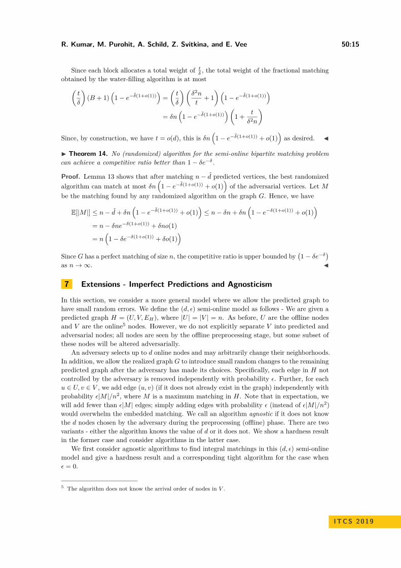
I Theorem 15. In the (d, ε) semi-online model with d < n/4, no (randomized) agnosticalgorithm can find a matching of size more than n− d− ε(n− 3d) +O(ε2n) in expectation,taken over the randomness of the algorithm and the randomness of the realized graph. Thisholds even if d is known in advance by the algorithm.

Proof. Assume n is even. Our hard instance consists of the following predicted graph H:For each integer i ∈ [0, n2 ), add edges (v2i+1, u2i+1), (v2i+1, u2i+2), and (v2i+2, u2i+2). Thiscreates n/2 connected components. See Figure 4 for an illustration.

The adversary chooses d components uniformly at random. Let A = {i1, i2, . . . , id} ⊂[0, n2 ) denote the indices of the d components selected by the adversary. For each index i ∈ A,the adversary then selects v2i+2 and changes its neighborhood so it only connects with u2i+1(instead of u2i+2).

For simplicity, let’s first consider the case when ε = 0. The algorithm can do no better thanpicking some p ∈ [0, 1], and matching v2i+1 to u2i+1 with probability p, and matching v2i+1to u2i+2 otherwise, for all i. The algorithm then matches v2i+2 to its neighbor, if possible.Now, for all i ∈ A (components selected by the adversary), this gets an expected matchingof size p+ 2(1− p) = 2− p. On the other hand, for all i /∈ A, the expected matching is size2p+(1−p) = 1+p. Since there are d components with an adversary and n/2−d componentswithout, this gives a total matching of size (2− p)d+ (1 + p)(n/2− d) = n/2 + d+ p(n2 − 2d).This is maximized when p = 1 (since d < n/4) to yield a matching of size n− d.

When ε > 0, the algorithm still should set p = 1; if the desired edge is removed, then thealgorithm will match with whatever node is available. Components with an adversarial nodegain an edge in the matching when the edge (v2i+1, u2i+1) is removed since the algorithmis forced into the right choice; if both edges (v2i+1, u2i+1) and (v2i+1, u2i+2) are removed,we neither gain nor lose. The expected gain is ε− ε2. Components without an adversarialnode lose an edge in the matching whenever either edge (v2i+1, u2i+1) or edge (v2i+2, u2i+2)is removed, and they lose an additional edge if all three edges of the component are removed.So the expected loss is 2ε− ε2 + ε3 Since there are d components with adversarial nodes andn/2− d without, this is a total of loss of

−d(ε− ε2) + (n/2− d)(2ε− ε2 + ε3) = ε(n− 3d)−O(ε2n)

Hence, the total matching is size n− ε(n− 3d) +O(ε2n), as claimed. J

R. Kumar, M. Purohit, A. Schild, Z. Svitkina, and E. Vee 50:17

I Theorem 16. Given a predicted graph H with a perfect matching, suppose there are dadversarial nodes and ε = 0 as described above in the (d, ε) semi-online model. Then there isan agnostic algorithm that does not know d that finds a matching of expected size n− d.

Proof. Before any online nodes arrive, find a perfect matching M in H. In the online stage,as each node v arrives, we attempt to identify v with an online node in the predicted graphwith the same neighborhood, and match v according to M . If no node in the predicted graphhas neighborhood identical to v, we know that v is adversarial and we can simply leave itunmatched. (Note that adversarial nodes can mimic non-adversarial nodes, but it doesn’tactually hurt us since they are isomorphic.) The predicted matching had size n, and we loseone edge for each adversarial node, so the obtained matching has size n− d. J

7.1 Fractional matchings for predictions with errorsIn this section, we show that we can find an almost optimal fractional matching for the (d, ε)semi-online matching problem.

We use a result from [22], which gives a method of reconstructing a fractional matchingusing only the local structure of the graph and a single stored value for each offline node.They provide the notion of a reconstruction function. Their results extend to a variety oflinear constraints and convex objectives, but here we need only a simple reconstructionfunction. For any positive integer k, define gk : (R+

0 )k → (R+0 )k by

gk(α1, α2, . . . , αk) = (α1 −max(0, z), α2 −max(0, z), . . . , αk −max(0, z))

where z is a solution to∑j min(max(0, αj − z), 1) = 1.

The reconstruction function g is this family of functions. Note that this is well-defined:there is always a solution z between −1 and the largest αj , and the solution is unique unlessz ≤ 0.

The result of [22] assigns a value αu to each u in the set of offline nodes, and reconstructsa matching on the fly as each online node arrives, using only the neighborhood of the onlinenode and the stored α values. Crucially, the reconstruction assigns reasonable values evenwhen the neighborhood is different than predicted. In this way, it is robust to small changesin the graph structure.

I Lemma 17 (Restated from [22]). Let gki be defined as above, and let H = (U, V,EH) bea bipartite graph with a perfect matching of size n = |U | = |V |. Then there exist values αufor each u ∈ U (which can be found in polynomial time) such that the following holds: Forall v ∈ V , define xui,v = gi(αu1 , αu2 , . . . αuk), where u1, u2, . . . , uk is the neighborhood of v.Then x defines a fractional matching on H with weight n.

Interested readers can find the proof in the full version. Given this reconstructiontechnique, we can now describe the algorithm:

In the preprocessing phase, find the αu values for all u ∈ U using Lemma 17.In the online phase, for each online node v, compute x̃ui,v = gi(αu1 , . . . , αuk), whereu1, . . . , uk ∈ ΓG(v), as described above. Assign weight x̃ui,v to the edge from ui to v; ifthat would cause node ui to have more than a total weight 1 assigned to it, just assign asmuch as possible.

Note that we make the online computation based on the neighborhood in G, the realizedgraph, although the αu values were computed based on H, the predicted graph. We havethe following.

ITCS 2019

50:18 Semi-Online Bipartite Matching

I Theorem 18. In the (d, ε) semi-online matching problem in which the predicted graphhas a perfect matching, there is a deterministic agnostic algorithm that gives a fractionalmatching of size n(1− 2ε− δ) in expectation, taken over the randomized realization of thegraph. The algorithm does not know the value of d or the value of ε in advance.

Proof. If the realized graph were exactly as predicted, we would give the fractional assignmentx guaranteed in Lemma 17, which has weight n. However, the fractional matching that isactually realized is somewhat different. For each online node that arrives, we treat it thesame whether it is adversarial or not. But we have a few cases to consider for analysis:

Case 1: The online node v is adversarial. In this case, we forfeit the entire weight of 1 inthe matching. We may assign some fractional matching to incident edges. However, wecount this as ‘excess’ and do not credit it towards our total. In this way, we lose at mostδn total weight.Case 2: The online node v is not adversarial, but it has extra edges added through arandom process. There are at most εn such nodes in expectation. In this case, we treatthem the same as adversarial. We forfeit the entire weight of 1, and ignore the ‘excess’assignment. This loses at most εn total weight in expectation.Case 3: The online node v is as exactly as predicted. In this case, we correctly calculatexuv for each u ∈ Γ(v). Further, we assign xuv to each edge, unless there was already‘excess’ there. Since we never took credit for this excess, we will take xuv credit now. Sowe do not lose anything in this case.Case 4: The online node v is as predicted, except each edge is removed with probabilityε (and no edges are added). In this case, when we solve for z, we find a value thatis bounded above by the true z. The reason is that in the predicted graph, we solved∑u∈Γ(v) min(max(0, αu − z), 1) = 1 for z when computing g. In the realized graph, this

same sum has had some of its summands removed, meaning the solution in z is at mostwhat it was before. So the value of x̃uv that we calculate is at least xuv for all u in therealized neighborhood. We take a credit of xuv for each of these, leaving the rest asexcess. Note that we have assigned 0 to each edge that was in the predicted graph butmissing in the realized graph. Since each edge goes missing with probability ε, this is atotal of at most εn in expectation.

So, the total amount we lose in expectation is 2εn+ δn. Since the matching in the predictedgraph has weight n, the claim follows. J

7.2 Semi-Online Algorithms For Ski RentalIn this section, we consider the semi-online ski rental problem. In the classical ski rentalproblem, a skier needs to ski for an unknown number of days and on each day needs todecide whether to rent skis for the day at a cost of 1 unit, or whether to buy skis for ahigher cost of b units and ski for free thereafter. We consider a model where the skier hasperfect predictions about whether or not she will ski on a given day for a few days in thetime horizon. In addition, she may or may not ski on the other days. For instance, say theskier knows whether or not she’s skiing for all weekends in the season, but is uncertain ofthe other days. The goal is to design an algorithm for buying skis so that the total cost ofskiing is competitive with respect to the optimal solution for adversarial choices for all thedays for which we have no predictions.

Let x denote the number of days that the predictions guarantee the skier would ski.Further, it is more convenient to work with the fractional version of the problem so that itcosts 1 unit to buy skis and renting for z (fractional) days costs z units. In this setting, we

R. Kumar, M. Purohit, A. Schild, Z. Svitkina, and E. Vee 50:19

know in advance that the skier will ski for at least x days. There is a randomized algorithmthat guarantees a competitive ratio of 1/(1 − (1 − x)e−(1−x)). Our analysis is a minorextension of an elegant result of [11].

I Theorem 19. There is a e

e− (1− x)ex competitive randomized algorithm for the semi-online ski-rental problem where x is a lower bound of the number of days the skier will ski.

Proof. Without loss of generality, we can assume that all the days with a prediction occurbefore any of the adversarial days arrive. Otherwise, the algorithm can always pretend as ifthe predictions have already occurred, since only the number of skiing days is important andnot their order. Recall that x denotes the number of days that the predictions guarantee theskier would ski. Let u ≥ x be the actual number of days (chosen by the adversary) that shewill ski. Since buying skis costs 1, the optimal solution has a cost of min(u, 1). Clearly, ifx ≥ 1, we must always buy the skis immediately and hence we assume that 0 ≤ x < 1 in therest of the section. Further, even the optimal deterministic algorithm buys skis once z = 1,so we may assume that u ≤ 1.

Let px(z) denote the probability that we buy the skis on day z, and let q(x) denotethe probability that we buy skis immediately. Recall that px is implicitly a function of theprediction x. Given a fixed number of days to ski u, we can now compute the expected costof the algorithm as

Cost(x, u) = q(x) +∫ u

0(1 + z) · px(z)dz +

∫ 1

u

u · px(z)dz

Our goal is to choose a probability distribution p so as to minimize Cost(x, u)/min(u, 1)while the adversary’s goal is to choose u to maximize the same quantity. We will choose pxand q so that Cost(x, u)/min(u, 1) is constant with respect to u. As we noted, u ≤ 1, somin(u, 1) = u. Setting the Cost(x, u) = c · u for constant c and taking the derivative withrespect to u twice gives us

0 = ∂

∂upx(u)− px(u)

Of course, px must also be a valid probability distribution. Thus, we set px(z) = (1− q(x)) ·ez

e− exfor z ≥ x. For z < x, we set px(z) = 0 since there is no reason to buy skis while

z < x if we did not already buy it immediately.Recalling that we set Cost(x, u) = c ·u, we can substitute px(z) and solve for q(x), finding

q(x) = xex

e− (1− x)ex

Hence, the competitive ratio is thus given by

Cost(x, u)u

= 1u

(q(x) + 1− q(x)

e− ex

∫ u

x

(1 + z)ezdz + 1− q(x)e− ex

∫ 1

u

u · ezdz)

Substitute q(x), and after some manipulation, this becomes

Cost(x, u)u

= e

e− (1− x)ex

Note that when x = 0, this becomes the classic ski rental problem, and the above bound ise/(e− 1), as expected. J

ITCS 2019

50:20 Semi-Online Bipartite Matching

References1 S. Albers and M Hellwig. Semi-online scheduling revisited. Theor. Comput. Sci., 443:1–9,

2012.2 J. Balogh and J Békési. Semi-on-line bin packing: a short overview and a new lower bound.

Cent. Eur. J. Oper. Res., 21(4):685–698, 2013.3 Hans-Joachim Böckenhauer, Dennis Komm, Rastislav Královic, Richard Královic, and To-

bias Mömke. On the Advice Complexity of Online Problems. In ISAAC, pages 331–340,2009.

4 Allan Borodin and Ran El-Yaniv. Online Computation and Competitive Analysis. Cam-bridge University Press, 2005.

5 Sebastien Bubeck and Aleksandrs Slivkins. The best of both worlds: Stochastic and ad-versarial bandits. In COLT, pages 42.1–42.23, 2012.

6 Rajiv Gandhi, Samir Khuller, Srinivasan Parthasarathy, and Aravind Srinivasan. De-pendent rounding and its applications to approximation algorithms. Journal of the ACM(JACM), 53(3):324–360, 2006.

7 Ashish Goel, Michael Kapralov, and Sanjeev Khanna. On the communication and streamingcomplexity of maximum bipartite matching. In SODA, pages 468–485. Society for Industrialand Applied Mathematics, 2012.

8 Pascal Van Hentenryck and Russell Bent. Online stochastic combinatorial optimization.The MIT Press, 2009.

9 Bala Kalyanasundaram and Kirk Pruhs. An optimal deterministic algorithm for onlineb-matching. Theor. Comput. Sci., 233(1-2):319–325, 2000. doi:10.1016/S0304-3975(99)00140-1.

10 Chinmay Karande, Aranyak Mehta, and Pushkar Tripathi. Online bipartite matching withunknown distributions. In STOC, pages 587–596, 2011.

11 Anna R. Karlin, Claire Kenyon, and Dana Randall. Dynamic TCP Acknowledgment andOther Stories about e/(e-1). Algorithmica, 36(3):209–224, 2003.

12 Anna R. Karlin, Mark S. Manasse, Lyle A. McGeoch, and Susan Owicki. Competitiverandomized algorithms for nonuniform problems. Algorithmica, 11(6):542–571, 1994.

13 Richard M Karp, Umesh V Vazirani, and Vijay V Vazirani. An optimal algorithm foron-line bipartite matching. In STOC, pages 352–358, 1990.

14 Ravi Kumar, Manish Purohit, and Zoya Svitkina. Improving Online Algorithms Using MLPredictions. In NIPS, 2018.

15 Euiwoong Lee and Sahil Singla. Maximum Matching in the Online Batch-Arrival Model.In IPCO, pages 355–367, 2017.

16 Thodoris Lykouris and Sergei Vassilvitskii. Competitive caching with machine learnedadvice. In ICML, pages 3302–3311, 2018.

17 Mohammad Mahdian, Hamid Nazerzadeh, and Amin Saberi. Online optimization withuncertain information. ACM Trans. Algorithms, 8(1):2:1–2:29, 2012.

18 Mohammad Mahdian and Qiqi Yan. Online bipartite matching with random arrivals: anapproach based on strongly factor-revealing LPs. In STOC, pages 597–606, 2011.

19 Andres Muñoz Medina and Sergei Vassilvitskii. Revenue Optimization with ApproximateBid Predictions. In NIPS, pages 1856–1864, 2017.

20 Aranyak Mehta. Online Matching and Ad Allocation. Foundations and Trends® in Theor-etical Computer Science, 8(4):265–368, 2013.

21 Vahab S. Mirrokni, Shayan Oveis Gharan, and Morteza Zadimoghaddam. Simultaneousapproximations for adversarial and stochastic online budgeted allocation. In SODA, pages1690–1701, 2012.

22 Erik Vee, Sergei Vassilvitskii, and Jayavel Shanmugasundaram. Optimal online assignmentwith forecasts. In EC, pages 109–118, 2010.