Semi-Matchings for Bipartite Graphs and

Load Balancing

Nicholas J. A. Harvey a Richard E. Ladner b Laszlo Lovasz c

Tami Tamir d

aMIT Computer Science and Artificial Intelligence Laboratory, Cambridge, MA.E-mail: nickh@mit.edu

bDepartment of Computer Science and Engineering, University of Washington,Seattle, WA, USA. E-mail: ladner@cs.washington.edu

cMicrosoft Research, Redmond, WA, USA. E-mail: lovasz@microsoft.comdDepartment of Computer Science and Engineering, University of Washington,

Seattle, WA, USA. E-mail: tami@cs.washington.edu

Abstract

We consider the problem of fairly matching the left-hand vertices of a bipartitegraph to the right-hand vertices. We refer to this problem as the optimal semi-matching problem; it is a relaxation of the known bipartite matching problem. Wepresent a way to evaluate the quality of a given semi-matching and show that,under this measure, an optimal semi-matching balances the load on the right handvertices with respect to any Lp-norm. In particular, when modeling a job assignmentsystem, an optimal semi-matching achieves the minimal makespan and the minimalflow time for the system.

The problem of finding optimal semi-matchings is a special case of certain schedul-ing problems for which known solutions exist. However, these known solutions arebased on general network optimization algorithms, and are not the most efficient wayto solve the optimal semi-matching problem. To compute optimal semi-matchingsefficiently, we present and analyze two new algorithms. The first algorithm gener-alizes the Hungarian method for computing maximum bipartite matchings, whilethe second, more efficient algorithm is based on a new notion of cost-reducing paths.Our experimental results demonstrate that the second algorithm is vastly superiorto using known network optimization algorithms to solve the optimal semi-matchingproblem. Furthermore, this same algorithm can also be used to find maximum bipar-tite matchings and is shown to be roughly as efficient as the best known algorithmsfor this goal.

Key words: bipartite graphs, load-balancing, matching algorithms,optimal algorithms, semi-matching

Preprint submitted to Elsevier Science 21 January 2005

1 Introduction

One of the classical combinatorial optimization problems is finding a maximummatching in a bipartite graph. The bipartite matching problem has numerouspractical applications [1, Section 12.2], and many efficient, polynomial timealgorithms for computing solutions [2] [3] [4]. Formally, a bipartite graph is agraph G = (U ∪V,E) in which E ⊆ U ×V . A matching in G is a set of edges,M ⊆ E, such that each vertex in U ∪ V is an endpoint of at most one edge inM . In other words, each vertex in U is matched with at most one vertex in Vand vice-versa.

In this paper we consider a relaxation of the maximum bipartite matchingproblem. We define a semi-matching to be a set of edges, M ⊆ E, such thateach vertex in U is an endpoint of exactly one edge in M . Clearly a semi-matching does not exist if there are isolated U -vertices, so we require thateach U -vertex in G have degree at least 1. Note that it is trivial to find asemi-matching — simply match each U -vertex with an arbitrary V -neighbor.Semi-matchings were previously considered in [5], with the objective of find-ing semi-matchings of maximum weight. We consider a different optimizationobjective: finding semi-matchings that match U -vertices with V -vertices asfairly as possible, that is, minimizing the variance of the matching edges ateach V -vertex.

Our work is motivated by the following load balancing problem: We are givena set of tasks and a set of machines, each of which can process a subset of thetasks. Each task requires one unit of processing time, and must be assigned tosome machine that can process it. The tasks are to be assigned to machines ina manner that minimizes some optimization objective. One possible objectiveis to minimize the makespan of the schedule, which is the maximal number oftasks assigned to any given machine. Another possible goal is to minimize theaverage completion time, or flow time, of the tasks. A third possible goal isto maximize the fairness of the assignment from the machines’ point of view,i.e., to minimize the variance of the loads on the machines.

These load balancing problems have received intense study in the online set-ting, in which tasks arrive and leave over time [6]. In this paper we considerthe offline setting, in which all tasks are known in advance. Problems fromthe online setting may be solved using an offline algorithm if the algorithm’sruntime is significantly faster than the tasks’ arrival/departure rate, and tasksmay be reassigned from one machine to another without expense. In partic-ular, the second algorithm we present can incrementally update an existingassignment after task arrivals or departures.

One example of an online load balancing problem that can be efficiently solved

2

by an offline solution comes from the Microsoft Active Directory system [7],which is a distributed directory service. Corporate deployments of this systemcommonly connect thousands of servers in geographically distributed branchoffices to servers in a central “hub” data center. Servers in the branch officesmust periodically replicate with the servers in the hub, which means to ex-change modified data between the servers to ensure that all servers have aconsistent copy of the database. However, there are constraints on which hubservers a given branch server may replicate with. The database is commonlypartitioned according to corporate divisions, such as “American Division” and“European Division”. Each branch server must replicate with any hub serverthat also stores the branch server’s database partition. Thus, the assignmentof branch servers to hub servers for the purpose of replication may be viewedas a constrained load balancing problem: the branch servers are the “tasks”,the hub servers are the “machines”, and the database partitions induce theconstraints. Since servers are only rarely added or removed, and servers canbe efficiently reassigned to replicate with another server, this load balancingproblem is solvable by the offline solutions that we present herein.

Load balancing problems of the form described above can be represented asinstances of the semi-matching problem as follows. Each task is represented bya vertex u ∈ U , and each machine is represented by a vertex v ∈ V . There is anedge u, v if task u can be processed by machine v. Any semi-matching in thegraph determines an assignment of the tasks to the machines. Furthermore,we show that a semi-matching that is as fair as possible gives an assignment oftasks to machines that simultaneously minimizes the makespan and the flowtime.

The primary contributions of this paper are: (1) the semi-matching model forsolving load balancing problems of the form described above, (2) two efficientalgorithms for computing optimal semi-matchings, and (3) a new algorithmicapproach for the bipartite matching problem. We also discuss in Section 2 rep-resentations of the semi-matching problem as network optimization problems,based on known solutions to scheduling problems. Section 3 proves several im-portant properties of optimal semi-matchings. One of these properties providesa necessary and sufficient condition for a semi-matching to be optimal. Specifi-cally, we define a cost-reducing path, and show that a semi-matching is optimalif and only if no cost-reducing path exists. Sections 4 and 5 present two algo-rithms for computing optimal semi-matchings; the latter algorithm uses theapproach of identifying and removing cost-reducing paths. Finally, Section 6describes an experimental evaluation of our algorithms against known algo-rithms for computing optimal semi-matchings and maximum bipartite match-ings.

3

2 Preliminaries

2.1 Definitions and Problem Statement

Let G = (U ∪ V,E) be a simple bipartite graph with U the set of left-handvertices, V the set of right-hand vertices, and edge set E ⊆ U ×V . We denoteby n and m the sizes of the left-hand and the right-hand sides of G respectively:i.e., n = |U | and m = |V |. Since our work is motivated by a load balancingproblem, we frequently refer to the U -vertices as “tasks” and to the V -verticesas “machines”.

We define a set M ⊆ E to be a semi-matching if each vertex u ∈ U is incidentwith exactly one edge in M . Note that isolated U -vertices can not be matchedwith any V -vertex, therefore we assume that all of the vertices in U have degreeat least 1. A semi-matching gives an assignment of each task to a machine thatis capable of processing it.

For v ∈ V , let deg(v) denote the degree of vertex v; in load balancing terms,deg(v) is the number of tasks that machine v is capable of executing. LetdegM(v) denote the number of edges in M that are incident with v; in loadbalancing terms, degM(v) is the number of tasks assigned to machine v. Wefrequently refer to degM(v) as the load on vertex v. Note that if several tasksare assigned to a machine then one task completes its execution after one timeunit, the next task after two time units, etc. However, semi-matchings do notspecify the order in which the tasks are to be executed.

We define costM(v) for a vertex v ∈ V to be

degM (v)∑

i=1

i =(degM(v) + 1)degM(v)

2.

This expression gives the total latency experienced by all tasks assigned tomachine v. The total cost of a semi-matching M is defined to be T (M) =∑m

i=1 costM(vi); this expression gives the flow time of the tasks’ schedule [8]. Asemi-matching with minimum total cost is called an optimal semi-matching.We show in Section 3 that an optimal semi-matching is also optimal with re-spect to other optimization objectives, such as maximizing the load balance onthe machines (by minimizing, for any p, the Lp-norm of the load-vector), min-imizing the variance of the machines’ load, and the minimizing the maximalmachine load.

For a given semi-matching M in G, define an alternating path to be a se-quence of edges P = (v1, u1, u1, v2, . . . , uk−1, vk) with vi ∈ V , ui ∈ U ,and vi, ui ∈ M for each i. For convenience, we sometimes treat paths as

4

a sequence of vertices (v1, u1, . . . , uk−1, vk). The notation A ⊕ B denotes thesymmetric difference of sets A and B; that is, A ⊕ B = (A \ B) ∪ (B \ A).Note that if P is an alternating path relative to a semi-matching M thenP ⊕ M is also a semi-matching, derived from M by switching matching andnon-matching edges along P . This switching process decreases the load onv1, increases the load on vk, and does not affect the load on any other vi.If degM(v1) > degM(vk) + 1 then P is called a cost-reducing path relative toM . Cost-reducing paths are so named because switching matching and non-matching edges along P yields a semi-matching P ⊕M whose cost is less thanthe cost of M . Specifically,

T (P ⊕ M) = T (M) − (degM(v1) − degM(vk) − 1).

2.2 Related Work

The maximum bipartite matching problem is known to be solvable in polyno-mial time using a reduction from maximum flow [1] [9] or by the Hungarianmethod [4] [5, Section 5.5]. Push-relabel algorithms are widely considered tobe the fastest algorithms in practice for this problem [2].

The load balancing problems we consider in this paper can be represented asrestricted cases of scheduling on unrelated machines. These scheduling prob-lems specify for each job j and machine i the value pi,j, which is the time ittakes machine i to process job j. When pi,j ∈ 1,∞ ∀i, j, this yields an in-stance of the semi-matching problem, as described in Section 2.3. In standardscheduling notation [10], this problem is known as R | pi,j ∈ 1,∞ | ∑

j Cj.Algorithms are known for minimizing the flow time of jobs on unrelated ma-chines [1, Application 12.9] [11] [8]; these algorithms are based on networkflow formulations.

The online version of this problem, in which the jobs arrive sequentially andmust be assigned upon arrival, has been studied extensively in recent years[12] [13] [14]. A comprehensive survey of the various models, and differentobjective functions is given in [6].

Optimal semi-matchings were concurrently and independently studied by Abra-ham [15, Section 4], under the name “balanced matchings”. His work containsa proof of our Theorem 13 and presents an algorithm for finding optimal semi-matchings. His algorithm differs from our algorithms ASM1 and ASM2, but hastheoretical performance similar to that of ASM1.

5

2.3 Representation as Known Optimization Problems

The optimal semi-matching problem can be represented as special instancesof two well-known optimization problems: weighted assignment and min-costmax-flow. However, Section 6 shows that the performance of the resulting al-gorithms is inferior to the performance of our algorithms presented in sections4 and 5.

Recall that the scheduling problem R | | ∑

j Cj, and in particular the casein which pi,j ∈ 1,∞, can be solved optimally [11] [8]. We now show thatthe optimal semi-matching problem can be reduced to the scheduling problemR | pi,j ∈ 1,∞ | ∑

j Cj. A semi-matching instance can be represented asa scheduling problem instance as follows: Each U -vertex represents a job,and each V -vertex represents a machine. For any job j and machine i, weset pi,j = 1 if the edge uj, vi exists, and otherwise pi,j = ∞. Clearly, anyfinite schedule for the scheduling problem determines a feasible semi-matching.In particular, a schedule that minimizes the flow time determines an optimalsemi-matching. Thus, an algorithms for R || ∑

j Cj can solve the optimal semi-matching problem. We note that current optimal algorithms for R || ∑

j Cj areusing as a subroutine a weighted assignment algorithm for a bipartite graphhaving n + nm vertices [11] [8].

The min-cost max-flow problem is one of the most important combinatorialoptimization problems [1]. Indeed, the weighted assignment problem can bereduced to min-cost max-flow problem. Thus, from the above discussion, itshould be clear that a semi-matching problem instance can be recast as amin-cost max-flow problem. We now describe an alternative, more compact,transformation of the optimal semi-matching problem to a min-cost max-flowproblem.

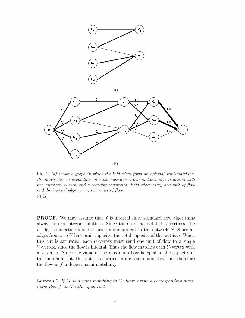
Given G = (U ∪V,E), a bipartite graph giving an instance of a semi-matchingproblem, we show how to construct a network N such that a min-cost max-flowin N determines an optimal semi-matching in G. The network N is constructedfrom G by adding at most |U |+2 vertices and 2|U |+ |E| edges (see Figure 1).The additional vertices are a source s, a sink t, and a set of “cost centers”C = c1, . . . , c∆, where ∆ ≤ |U | is the maximal degree of any V -vertex.Edges with cost 0 and capacity 1 connect s to each of the vertices in U . Theoriginal edges connecting U and V are directed from U to V and are given cost0 and capacity 1. For each v ∈ V , v is connected to cost centers c1, . . . , cdeg(v)

with edges of capacity 1 and costs 1, 2, . . . , deg(v) respectively. Edges withcost 0 and infinite capacity connect each of the cost centers to the sink, t.

We now prove the validity of this reduction.

Lemma 1 If f is a maximum flow in N then f determines a semi-matching

6

(a)

∞

∞

∞

(b)

Fig. 1. (a) shows a graph in which the bold edges form an optimal semi-matching.(b) shows the corresponding min-cost max-flow problem. Each edge is labeled withtwo numbers: a cost, and a capacity constraint. Bold edges carry one unit of flowand doubly-bold edges carry two units of flow.

in G.

PROOF. We may assume that f is integral since standard flow algorithmsalways return integral solutions. Since there are no isolated U -vertices, then edges connecting s and U are a minimum cut in the network N . Since alledges from s to U have unit capacity, the total capacity of this cut is n. Whenthis cut is saturated, each U -vertex must send one unit of flow to a singleV -vertex, since the flow is integral. Thus the flow matches each U -vertex witha V -vertex. Since the value of the maximum flow is equal to the capacity ofthe minimum cut, this cut is saturated in any maximum flow, and thereforethe flow in f induces a semi-matching.

Lemma 2 If M is a semi-matching in G, there exists a corresponding maxi-

mum flow f in N with equal cost.

7

PROOF. The flow f is defined as follows: for each u ∈ U , one flow-unit issent from s to u and then to the V -vertex to which u is matched. For eachv ∈ V , each flow unit arriving at v is sent to the available edge of least costconnecting v with a cost-center, and then to t. By definition of the edges fromV to C, the total cost of the flow on those edges is

∑mi=1

∑degM (vi)j=1 j. Since all

other edges have zero cost, this is also the cost of the whole flow.

In particular, if the optimal semi-matching has cost Copt then the min-costmax-flow in N has cost Copt. We now extend Lemma 1 to show that a min-cost max-flow in N determines a semi-matching with the same cost.

Lemma 3 If fopt is a minimum-cost maximum-flow in N and M is the cor-

responding semi-matching in G, then the cost of fopt equals the total cost of

M .

PROOF. As before, we assume that fopt is integral. In any minimum-costflow, the flow-units leaving each v ∈ V must be sent to the cost-centers usingedges with least cost. That is, if f(vi) is the total amount of flow leaving vi

then the flow is sent to cost-centers c1, . . . , cf(vi). Since all the other edges in

N have cost zero, the total cost of the flow is∑m

i=1

∑f(vi)j=1 j. In the matching

M induced by fopt, each u ∈ U is matched to a vi ∈ V if and only if there isone flow unit on the edge (u, vi). Therefore, f(vi) = degM(vi), and the totalcost of fopt is exactly T (M).

3 Properties of Optimal Semi-Matchings

This section proves various important properties of optimal semi-matchings.Section 3.1 characterizes when a semi-matching is optimal. Section 3.2 gener-alizes the notion of optimality to other cost functions. Section 3.3 proves thatan optimal semi-matching always contains a maximum matching and discussesvarious consequences. Section 3.4 proves that an optimal semi-matching is alsooptimal with respect to any Lp-norm and the L∞-norm.

3.1 Characterization of Optimal Semi-Matchings

An important theorem from network flow theory is that a maximum flow hasminimum cost if and only if no negative-cost cycle exists [1, Theorem 3.8]. Wenow prove an analogous result for semi-matchings. In Section 5 we describethe Algorithm ASM2 which is based on this property.

8

Theorem 4 A semi-matching M is optimal if and only if no cost-reducing

path relative to M exists.

PROOF. Let G be an instance of a semi-matching problem, and let M be asemi-matching in G. Clearly if M is optimal then no cost-reducing path canexist. We show that a cost-reducing path must exist if M is not optimal.

Let O be an optimal semi-matching in G, chosen such that the symmetricdifference O ⊕ M = (O \ M) ∪ (M \ O) is minimized. Assume that M is notoptimal, implying that M has greater total cost than O: i.e., T (O) < T (M).Recall that degO(v) and degM(v) denote the number of U -vertices matchedwith v by O and M respectively. Let Gd be the subgraph of G induced by theedges of O ⊕M . Color with green the edges of O \M and with red the edgesof M \O. Direct the green edges from U to V and the red edges from V to U .

Claim 5 The graph Gd is acyclic, and for every directed path P in Gd from

v1 ∈ V to v2 ∈ V , we have degO(v2) ≤ degO(v1).

PROOF. Let P = (v1, . . . , v2) be a directed path in Gd. By the choice ofdirections for the edges, P must consist of alternating red and green edges. IfdegO(v2) > degO(v1) + 1 then P (in reverse order) is a cost-reducing path forO, in contradiction to the optimality of O. If degO(v2) = degO(v1) + 1, thenby alternating the assignment of the U -vertices along P we get an optimalassignment with smaller symmetric difference from M , again in contradictionto the choice of O. Therefore, we must have that degO(v2) ≤ degO(v1). Asimilar argument shows that Gd is also acyclic.

Both O and M are semi-matchings, implying that∑

v degO(v) =∑

v degM(v) =|U |. Since T (O) < T (M), there must exist v1 ∈ V such that degM(v1) >degO(v1). Starting from v1, we build an alternating red-green path P ′ as fol-lows. (1) From an arbitrary vertex v ∈ V , if degM\O(v) ≥ 1 and degM(v) ≥degM(v1) − 1, we build P ′ by following an arbitrary red edge directed outfrom v. (2) From an arbitrary vertex u ∈ U , we build P ′ by following thesingle green edge directed out from u. Such a green edge must always exist.(3) Otherwise, we stop.

By Claim 5, Gd is acyclic and therefore P ′ is well-defined and finite. Let v2 ∈ Vbe the final vertex on the path. There are two cases.

Case 1: degM(v2) < degM(v1)− 1. Thus P ′ is a cost-reducing path relativeto M .

Case 2: degM\O(v2) = 0. In this case, we know that degM(v2) < degO(v2)since P ′ arrived at v2 via a green edge. By Claim 5, we must also have

9

that degO(v2) ≤ degO(v1). Finally, recall that v1 was chosen such thatdegO(v1) < degM(v1). Combining these three inequities yields: degM(v2) <degO(v2) ≤ degO(v1) < degM(v1). This implies that degM(v2) < degM(v1)−1, and so P ′ is a cost-reducing path relative to M .

Since P ′ is a cost-reducing path relative to M in both cases, the proof iscomplete.

3.2 Optimality with Respect to Other Cost Functions

So far we have considered only the objective of minimizing T (M) =∑m

i=1 costM(vi),

where costM(v) =∑degM (v)

i=1 i = (degM (v)+1)degM (v)2

. Recall that this expressiongives the flow time of the tasks’ schedule. In this section we show that in factour results capture a wider set of objectives, given by different cost functions.We show that an optimal semi-matching is optimal with respect to any of thesecost functions. In other words, an optimal semi-matching minimizes flow timeas well as many other important properties of the system.

Definition 6 A cost function for a matching M is a function costf (M) =∑m

i=1 f(degM(vi)), where f : R+ → R is a strictly convex function. If f is

weakly convex then costf (M) is called a weak cost function.

For example, T (M) is the cost function induced by the function f(x) =∑x

j=1 j = x(x + 1)/2.

Lemma 7 Let P be a cost-reducing path. For any cost function costf , switch-

ing matching and non-matching edges along P yields a semi-matching M ′ =P ⊕M such that costf (M

′) < costf (M). If costf is a weak cost function then

costf (M′) ≤ costf (M).

PROOF. First, we need the following property of convex functions:

Claim 8 If f is strictly convex then x > y implies f(x + 1) − f(x) > f(y +1) − f(y). If f is weakly convex then the inequality holds but is not strict.

PROOF. A property of strictly convex functions is that f(b)−f(a)b−a

< f(c)−f(a)c−a

<f(c)−f(b′)

c−b′if a < b < c and a < b′ < c (see, for example, [16]). Setting a = y,

b = y + 1, b′ = x and c = x + 1 we obtain that f(y + 1)− f(y) < f(x+1)−f(y)x+1−y

<

f(x+1)− f(x). If f is weakly convex then all stated inequalities hold but arenot strict.

10

Next, consider the matching M and the cost-reducing path P = (v1, . . . , vk).Let x = degM(v1) − 1 and y = degM(vk). The change in costf at v1 due toswitching edges along path P is f(x)−f(x+1). Similarly, the change in costf

at vk is f(y + 1) − f(y). Therefore

costf (M′) = costf (M) −

(

f(x + 1) − f(x))

+(

f(y + 1) − f(y))

.

Applying Claim 8 completes the proof.

Using Lemma 7 we can extend Theorem 4 as follows.

Theorem 9 Let M be a semi-matching. If costf is a strict cost function and

if M is optimal with respect to costf then no cost-reducing path relative to Mexists. The converse holds even if costf is a weak cost function: if no cost-

reducing path relative to M exists then M is optimal with respect to costf .

PROOF. Identical to the proof of Theorem 4.

Thus, if M is optimal with respect to a strict cost function then no cost-reducing path relative to M exists. Also, if M has no cost-reducing pathsthen M is optimal with respect to every cost function.

Corollary 10 A semi-matching M that is optimal with respect to any strict

cost function is optimal with respect to every cost function, strict or weak.

3.3 Optimal Semi-Matchings Contain Maximum Matchings

In this section, we prove that every optimal semi-matching must contain amaximum bipartite matching; furthermore, it is a simple process to find thesemaximum matchings. Thus, the problem of finding optimal semi-matchingsindeed generalizes the problem of finding maximum matchings.

Theorem 11 Let M be an optimal semi-matching in G. Then there exists

S ⊆ M such that S is a maximum matching in G.

PROOF. Given a semi-matching M (not necessarily an optimal one), we mayconstruct an ordinary matching (not necessarily a maximum one) by selectingone incident M -edge for each vertex v ∈ V . If there are ` vertices in V withdegM(v) > 0, then the resulting matching is of size `. Conversely, any matchingcan be extended to a semi-matching (not necessarily an optimal one) by adding

11

one arbitrary incident edge for any unmatched u in U . Thus, any matching,and in particular any maximum one, is contained in some semi-matching. Inorder to show that an optimal semi-matching contains a maximum matching,we show that an optimal semi-matching minimizes the number of unmatchedV -vertices (i.e., vertices v ∈ V with degM(v) = 0).

Define f : R+ → R such that f(x) = 0 for x ≤ 1 and f(x) = x − 1 for

x > 1. Note that f is weakly convex so costf is a weak cost function. LetM be an optimal semi-matching (i.e., with respect to T (M)). M is thereforeoptimal with respect to costf by Corollary 10. costf is defined such that ifdegM(v) > 0 then v contributes degM(v) − 1 to the total cost. Summing overall v ∈ V , costf (M) = n − `, where ` is the number of vertices in V with atleast one incident edge in M . Since M minimizes costf , it maximizes `. By ourprevious remarks, M contains a matching of size `, so M contains a maximummatching.

The converse of this theorem is not true. As demonstrated in Appendix C,not every maximum matching can be extended to an optimal semi-matching.

Corollary 12 Let M be an optimal semi-matching in G. Define α(M) to be

the number of right-hand vertices in G that are incident with at least one edge

in M . Then the size of a maximum matching in G is α(M).

In particular, if G has a perfect matching and M is an optimal semi-matchingin G, then M is a perfect matching. Corollary 12 yields a simple algorithm forcomputing a maximum matching from an optimal semi-matching M : for eachv ∈ V , if degM(v) > 1, select one arbitrary edge from M that is incident withv.

3.4 Optimality with Respect to Lp-norm and L∞-norm

Let xi = degM(vi) denote the load on machine i, that is, the number oftasks assigned to machine i. The Lp-norm of the vector X = (x1, . . . , xm) is‖X‖p = (

∑mi=1 xp

i )1/p. In this section we show that an optimal semi-matchingis optimal with respect to the Lp-norm of the vector X for any finite p; inother words, optimal semi-matchings minimize ‖X‖p of the load vector. (Allsemi-matchings have ‖X‖1 = |U |, and hence are optimal with respect to theL1-norm).

Theorem 13 Let 1 < p < ∞. A semi-matching is optimal if and only if it is

optimal with respect to the Lp-norm of its load vector.

12

PROOF. Fix any p > 1 and define fp(x) = xp. Note that fp is strictlyconvex so costfp

is a strict cost function. Let X be the load vector for M .Since ‖X‖p = costfp

(M)1/p, M optimizes ‖X‖p if and only if it optimizescostfp

. By Corollary 10, M is optimal with respect to costfpif and only if M

is an optimal semi-matching.

Another common measure for load balancing is the variance of the loads onthe machines. The following theorem shows that optimal semi-matchings arealso optimal for this objective.

Theorem 14 A semi-matching M is optimal if and only if Varv∈V degM(v)is minimized.

PROOF. Let µ = n/m be the mean of degM(v) where v ∈ V . DefinefVar(x) = (x−µ)2 and note that costfVar

is a strict cost function. By Corollary 10,M is optimal with respect to costfVar

if and only if M is an optimal semi-matching.

Another important optimization objective in practice is minimizing the makespan,which is the maximal load on any machine. This is achieved by minimizing theL∞-norm of the machines’ load vector X. As we show below, optimal semi-matchings do minimize the L∞-norm of X, and thus are an “ultimate” solutionthat simultaneously minimizes both the flow time and the makespan. Recallthat |V | = m and consider the function f∞ defined by f∞(x) = (m+1)x. Notethat costf∞ is a strict cost function.

Claim 15 A semi-matching that minimizes costf∞ minimizes the maximal

load on a single V -vertex.

PROOF. Let M be an assignment that minimizes costf∞ . Assume that Mdoes not minimize the maximal load on a single V -vertex, and that this ob-jective is achieved by a different assignment M ′. Let ∆ and ∆′ be the maxi-mal load on a single V -vertex in M and M ′ respectively. Thus, costf∞(M) ≥(m+1)∆ and costf∞(M ′) ≤ m(m+1)∆′

(at worst, all m of the V -vertices haveload ∆′). However, since ∆′ ≤ ∆−1, it follows that costf∞(M ′) < costf∞(M),which is a contradiction.

Theorem 16 An optimal semi-matching M is also optimal with respect to

the L∞-norm.

13

PROOF. Since costf∞ is a cost function, Corollary 10 implies that M isoptimal with respect to costf∞ . By Claim 15, this implies that M minimizesthe maximal load on a V -vertex. Therefore M is optimal with respect to theL∞-norm.

The converse of Theorem 16 is not valid; that is, minimizing the L∞-normdoes not imply minimization of other cost functions. The converse of Theorem16 fails to hold because the converse of Claim 15 does not hold: minimizingthe makespan does not necessarily minimize costf∞ . A semi-matching thatminimizes only the L∞-norm is given in Appendix C.

4 ASM1: An O(|U ||E|) Algorithm for Optimal Semi-Matchings

In this section we present our first algorithm, ASM1, for finding an optimalsemi-matching. The time complexity of ASM1 is O(|U ||E|), which is identicalto that of the Hungarian algorithm [4] [5, Section 5.5] for finding maximumbipartite matchings. Indeed, ASM1 is merely a simple modification of the Hun-garian algorithm, as we explain below.

The Hungarian algorithm for finding maximum bipartite matchings considerseach left-hand vertex u in turn and builds an alternating search tree, rootedat u, looking for an unmatched right-hand vertex (i.e., a vertex v ∈ V withdegM(v) = 0). If an unmatched right-hand vertex v is found, the matchingand non-matching edges along the u-v path are switched so that u and v areno longer unmatched.

Similarly, ASM1 maintains a partial semi-matching M , starting with the emptyset. In each iteration, it considers a left-hand vertex u and builds an alternatingsearch tree rooted at u, looking for a right-hand vertex v such that degM(v)is as small as possible. To build the tree rooted at u we perform a directedbreadth-first search in G starting from u, where edges in M are directed fromV to U and edges not in M are directed from U to V . We select in this treea path P from u to a least loaded V -vertex reachable from u. We increasethe size of M by forming P ⊕M ; in other words, we add to the matching thefirst edge in this path, and switch the next matching and non-matching edgesalong the remainder of the path. As a result, u is no longer unmatched anddegM(v) increases by 1.

We repeat this procedure of building a tree and extending the matching ac-cordingly for all of the vertices in U . Since each iteration matches a vertex inU with a single vertex in V and does not change degM(u) for any other u ∈ U ,the resulting selection of edges is indeed a semi-matching. The pseudocode of

14

this algorithm is given in Appendix A.

Interestingly, there is another way to characterize ASM1. Section 2.3 showedthat G can be represented as a network N in which a min-cost max-flow corre-sponds to an optimal semi-matching. One way to compute a min-cost max-flowin N is with the successive shortest path algorithm [1, Section 9.7]. RegardingG as a compact representation of N , ASM1 is an efficient implementation ofthe successive shortest path algorithm on G.

Theorem 17 Algorithm ASM1 produces an optimal semi-matching.

PROOF. We show that no cost-reducing path is created during the executionof the algorithm. In particular, no cost-reducing path exists at the end of theexecution; thus, by Theorem 4 the resulting matching is optimal.

Assume the opposite and let P ∗ = (v1, u1, . . . , vk−1, uk−1, vk), be the first cost-reducing path created by this algorithm. Let M1 be the matching after theiteration in which P ∗ is created. Thus, degM1

(v1) > degM1(vk) + 1. Without

loss of generality (by taking a sub-path of P ∗), we can assume that thereexists some x such that degM1

(v1) ≥ x+1, degM1(vi) = x,∀i ∈ 2, . . . , k− 1,

and degM1(vk) ≤ x − 1. Consider the last iteration in which the load on v1 is

increased. Let u′ be the U -vertex added to the assignment at this iteration. Bythe definition of the algorithm, v1 is a least loaded V -vertex reachable fromu′; thus, the search tree built for u′ includes only V -vertices with load at leastx; in particular, vk is not reachable from u′.

Given that the path P ∗ exists, at some iteration occurring after the one inwhich u′ is added, all the edges (ui, vi) of P ∗ are in the matching. Let u∗ bethe U -vertex, added after u′, whose addition to the assignment creates P ∗.We show a contradiction to the way u∗ is assigned. Specifically, we show thatwhen adding u∗, the algorithm increases the load on some vertex with load atleast x, while vk, whose load at that time is at most x − 1, is also reachablefrom u∗.

Claim 18 When u∗ is added, the load on vk is at most x− 1 and vk is in the

tree rooted at u∗.

PROOF. The load on any V -vertex can only increase during the algorithm.Since the load on vk in M1 is x−1, and u∗ is added before P ∗ exists, x−1 is anupper bound on the load on vk at the time u∗ is added. To see that vk is in T ∗,the search tree built during the assignment of u∗, recall the assumption thatthe path P ∗ is created by the assignment of u∗. Let (ui, vi) be the last edge(i.e., farthest from v1) of P ∗ that is added to the matching in this iteration.

15

Thus, vi is reachable from u∗, and since the edge (uj, vj) is already in thematching ∀j, i < j ≤ k, the suffix of P ∗ from vi to vk must also be in T ∗.

Claim 19 When u∗ is added, the load on some vertex with load at least x is

increased.

PROOF. Suppose the opposite. We show that a cost-reducing path existsbefore u∗ is added, contradicting our choice of P ∗ as the first cost-reducingpath created by the algorithm. Once again, we use the fact that P ∗ is createdwhen u∗ is added. Let (ui, vi) be the first edge (i.e., closest to v1) of P ∗ whichis added to the matching at this iteration. Thus, before adding u∗, the vertexvi is reachable from v1. Let P ′ = (u∗, . . . , v∗) be the path from u∗ to the leastloaded vertex in T ∗. Note that vi must appear in path P ′. Thus, the path fromv1 to vi can be extended to reach v∗ using the suffix of P ′ from vi to v∗. Allthe edges of this suffix are available before u∗ is added, since they were allavailable to T ∗. The load on v∗ must be at least x, otherwise the above pathfrom v1 to v∗ is a cost-reducing path which exists before P ∗.

Combining Claims 18 and 19 contradicts the execution of ASM1, and thereforeP ∗ cannot exist.

To bound the running time of ASM1, observe that there are exactly |U | iter-ations. Each iteration requires at most O(|E|) time to build the alternatingsearch tree and at most O(min|U |, |V |) time to switch edges along the al-ternating path. Thus the total time required is at most O(|U ||E|).

This O(|U ||E|) bound is the same upper-bound as for the Hungarian algo-rithm. However, in practice ASM1 is slower than the Hungarian algorithm be-cause it tends to build a very large search tree in each iteration. The followingsection presents another algorithm which is much more efficient in practice.

5 ASM2: An Efficient Practical Algorithm

This section describes ASM2, another algorithm for finding optimal semi-matchings. Our analysis of this algorithm’s runtime gives an upper boundof O(min|U |3/2, |U ||V | · |E|), which is worse than the bound of O(|U ||E|) foralgorithm ASM1. However, our analysis for ASM2 is loose; in practice, ASM2

performs much better than ASM1, as our experiments in Section 6 show.

Theorem 4 proves that a semi-matching is optimal if and only if the graph doesnot contain a cost-reducing path. ASM2 uses that result to find an optimal

16

Find an initial semi-matching, M

While there exists a cost-reducing path, P

Reduce the cost by switching the matching and non-matching

edges along path P

Fig. 2. Overview of ASM2

semi-matching. Figure 2 gives an overview of the ASM2 algorithm. Since eachiteration reduces the total cost by an integral amount, the cost can only bereduced a finite number of times, so this algorithm must terminate. Moreover,if the initial assignment is nearly optimal, the algorithm terminates after fewiterations.

As was the case for ASM1, network flows give an alternative characterizationof algorithm ASM2. As described in Section 2.3, G can be represented as anetwork N . Regarding G as a compact representation of N , ASM2 is an efficientimplementation of the generic cycle canceling algorithm [1, Section 9.6] on G.

Finding an Initial Semi-Matching: The first step of algorithm ASM2 isto determine an initial semi-matching, M . A simple approach would be toarbitrarily assign each left-hand vertex to a right-hand vertex. However, as ageneral rule, finding an initial matching with lower cost tends to reduce thenumber of iterations required to achieve optimal cost. Our experiments haveshown that the following greedy algorithm works well in practice.

First, the U -vertices are sorted by increasing degree. Each U -vertex is thenconsidered in turn and assigned to a V -neighbor with least load. In the caseof a tie, a V -neighbor with least degree is chosen. The purpose of consideringvertices with lower degree earlier is to allow more constrained vertices (i.e.,ones with fewer neighbors) to “choose” their matching vertices first. The samerule of choosing the least loaded V -vertex is also commonly used in the onlinecase [12]. However, in the online case it is not possible to sort the U -verticesor to know the degree of the V -vertices in advance. The pseudocode of thisalgorithm is given in Appendix B.

The total time required to find this initial matching is O(|E|), since everyedge is examined exactly once, and the sorting can be done using bucket sort.Our experiments have shown that sorting U is effective in practice at reducingthe cost of the initial matching, and hence reducing the number of iterationsrequired to achieve optimal cost.

Finding Cost-Reducing Paths: The critical operation of the ASM2 algo-rithm is the method for finding cost-reducing paths. As a simple approach,we can determine if a particular vertex v ∈ V is the initial vertex of a cost-reducing path simply by growing a depth-first search tree of alternating pathsrooted at v. To determine if G has any cost-reducing paths at all, it sufficesto perform m depth-first searches, one from each vertex v ∈ V . This simple

17

algorithm unfortunately performs much redundant work. The following claimleads to an approach for avoiding this redundant work.

Claim 20 Let v, w ∈ V be such that degM(v) ≥ degM(w) and there is an

alternating path from v to w. If there is no cost-reducing path starting from vthen there is no cost-reducing path starting from w.

PROOF. We prove the contrapositive. Since there is an alternating pathfrom v to w, any cost-reducing path starting from w can be extended to acost-reducing path starting from v.

Our algorithm for finding cost-reducing paths works as follows. First we finda vertex v ∈ V such that v has not been visited by any previous depth-firstsearches and degM(v) is maximum over all such vertices. To find a such avertex v quickly, the non-visited V -vertices are maintained sorted by theirload in an array of |U | + 1 buckets. Next we build a depth-first search tree ofalternating paths rooted at v in the usual manner. If this depth-first searchtree does not contain a cost-reducing path then Claim 20 shows that there isno cost-reducing path starting from any of the vertices that were visited. Sincethis algorithm considers each edge in G at most once and there are only |U |+1buckets, it finds a cost-reducing path or lack thereof in O(|U |+ |E|) = O(|E|)time.

After finding a cost-reducing path, we reduce the cost of the matching byswitching matching and non-matching edges along the path. This step clearlytakes O(|E|) time as well. Recall that this switching process only affects theload on the first and last vertices on the path.

Analysis of ASM2: As argued earlier, the initial matching can be found inO(|E|) time. Following this initial step, we iteratively find and remove cost-reducing paths. Identifying a cost-reducing path requires O(|E|) time. If acost-reducing path has been identified, then we switch matching and non-matching edges along that path, requiring O(min|U |, |V |) = O(|E|) time.Thus, the runtime of ASM2 is O(I · |E|), where I is the number of iterationsneeded to achieve optimality.

It remains to determine how many iterations are required. A simple boundof I = O(|U |2) may be obtained by observing that the worst possible initialmatching has total cost at most O(|U |2) and that each iteration reduces thecost by at least 1. We now derive an improved bound.

Theorem 21 ASM2 requires at most O(min|U |3/2, |U ||V |) iterations to achieve

optimality.

18

PROOF. For a given initial semi-matching, M0, assume that the V -verticesare sorted by load in non-increasing order, that is, degM0

(v1) ≥ . . . ≥ degM0(vm).

In each iteration, the algorithm identifies a cost-reducing path P = (va, . . . , vb).By switching matching and non-matching edges along this path we remove oneunit of load from va and add one unit to vb. This load balancing process canbe described as follows: Initially we have n towers of blocks, where the ith

tower consists of degM0(vi) blocks. Reducing the cost using path P amounts

to moving one block from the tower corresponding to va to the tower cor-responding to vb. We bound the number of iterations of ASM2 by boundingthe total number of possible block moves. Our proof is based on the followingproperties:

(1) Since we always move load units to a less loaded vertex, operations may beordered such that the V -vertices remain sorted in non-increasing order oftheir loads throughout the execution of ASM2. In other words, the towersare always sorted from highest to lowest.

(2) By the definition of cost-reducing paths, when moving a load unit fromva to vb, the load on va before the iteration is strictly greater than theload on vb after the iteration.

For any value of m, the total number of moves is at most nm since by theabove properties each block may be moved at most m times. If m >

√n, we

use a different argument. Consider the kth tower, corresponding to vk, wherek is arbitrary. By the first property, the maximum possible load on vk at anytime is n/k. Thus, the height of the kth tower is at most n/k. By the secondproperty, any block that we keep moving from tower k can be moved at mostn/k additional times before it arrives a tower with height 1 (and hence couldnever be moved again).

Thus, for any k, each block may be moved at most k+n/k times in total. Thetightest bound is obtained by choosing k = d√ne: Each block may be moved atmost 2

√n+1 times. Since each move of a block corresponds to one iteration of

ASM2, the number of iterations of ASM2 is O(n3/2). In conclusion, combiningthe nm bound that holds for arbitrary m with the improved bound for m >√

n, we may bound the total number of iterations by O(min|U |3/2, |U ||V |).

Remark: For graphs in which the optimal semi-matching cost is O(|U |), therunning time of ASM2 is O(|U ||E|). This bound holds since Awerbuch et al.[12] show that the cost of the greedy initial assignment is at most 4 ·T (MOPT );thus ASM2 needs at most O(|U |) iterations to achieve optimality.

Practical Considerations: The simplified pseudocode for ASM2 given inAppendix B suggests that each iteration builds a depth-first search forest andfinds a single cost-reducing path. In practice, a single DFS forest often con-

19

tains numerous vertex-disjoint cost-reducing paths. Thus, our implementationrepeatedly performs linear-time scans of the graph, growing the forest and re-moving cost-reducing paths. We repeatedly scan the graph until a scan findsno cost-reducing path, indicating that optimality has been achieved.

Our bound of O(min|U |3/2, |U ||V |) iterations is loose: Experiments showthat significantly fewer iterations are required in practice. We were able tocreate “bad” graphs, in which the number of iterations needed is Ω(|U |3/2);however, most of the cost-reducing paths in these graphs are very short, thuseach iteration takes roughly constant time. While our bound for ASM2 isworse than our bound for ASM1, we believe that the choice of ASM2 as thebest algorithm is justified already by its performance in practice, as describedin the next section.

Variants of ASM2, in which each iteration seeks a cost-reducing path withsome property (such as “maximal difference in load between first and lastvertex”), will also result in an optimal semi-matching. It is unknown whethersuch algorithms yield a better analysis than ASM2, or whether each iterationof such algorithms can be performed quickly in practice.

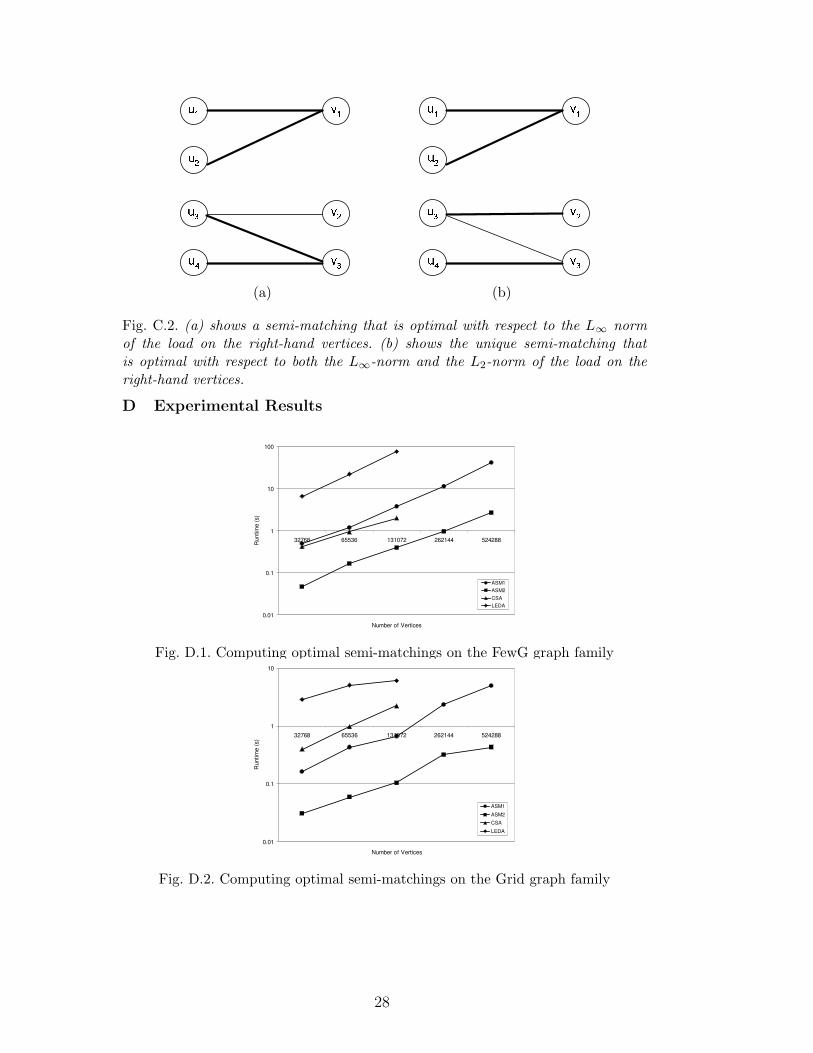
6 Experimental Evaluation

We implemented a program to execute ASM1, ASM2 and various known al-gorithms on a variety of “benchmark” input graphs. Our simulation programwas implemented in C and run on a 2.4GHz Pentium 4 machine with 512MBof RAM. Each input graph is a random graph from a particular family. Thegraph generators for each family, and the following descriptions of them, arefrom [2]. All graphs have |U | = |V |.

FewG and ManyG: The U -vertices and V -vertices are divided into k groupsof equal size. The FewG family has k = 32 and the ManyG family has k = 256.Each vertex in the jth group of U chooses y random neighbors from the (i−1)th

through (i + 1)th group of V , where y is binomially distributed with mean 5.

Grid: The graph is an approximate d-dimensional grid. d is chosen such thatthe average degree is roughly 6.

Hexa: The vertices on each side are partitioned into n/b blocks of size b. Onerandom bipartite hexagon is added between each block i on one side and eachof the blocks i+k on the other side, with |k| ≤ K for some K. The parametersb and K are chosen by the program in such a way that an average degree of6 is achieved (i.e., 3K/b = 6), but few pairs of hexagons have more than onevertex in common.

Hilo: The ith U -vertex is connected to the jth V -vertex, for all positive j with

20

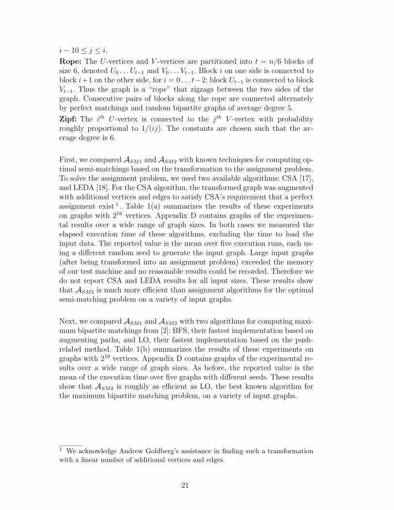
i − 10 ≤ j ≤ i.

Rope: The U -vertices and V -vertices are partitioned into t = n/6 blocks ofsize 6, denoted U0 . . . Ut−1 and V0 . . . Vt−1. Block i on one side is connected toblock i+1 on the other side, for i = 0 . . . t−2; block Ut−1 is connected to blockVt−1. Thus the graph is a “rope” that zigzags between the two sides of thegraph. Consecutive pairs of blocks along the rope are connected alternatelyby perfect matchings and random bipartite graphs of average degree 5.

Zipf: The ith U -vertex is connected to the jth V -vertex with probabilityroughly proportional to 1/(ij). The constants are chosen such that the av-erage degree is 6.

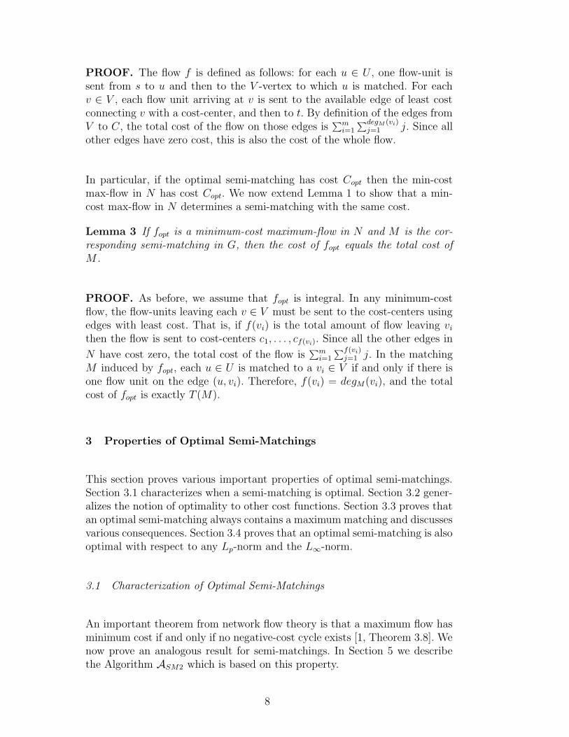
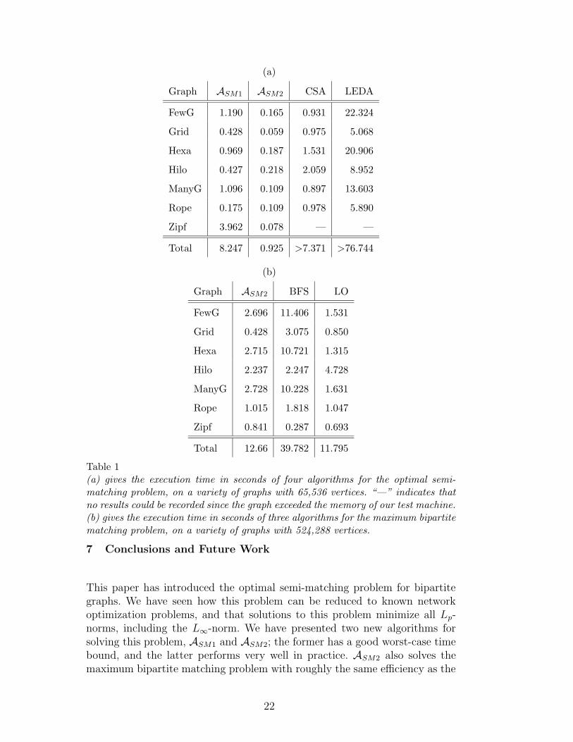
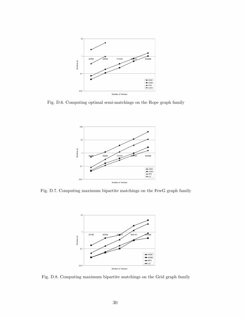
First, we compared ASM1 and ASM2 with known techniques for computing op-timal semi-matchings based on the transformation to the assignment problem.To solve the assignment problem, we used two available algorithms: CSA [17],and LEDA [18]. For the CSA algorithm, the transformed graph was augmentedwith additional vertices and edges to satisfy CSA’s requirement that a perfectassignment exist 1 . Table 1(a) summarizes the results of these experimentson graphs with 216 vertices. Appendix D contains graphs of the experimen-tal results over a wide range of graph sizes. In both cases we measured theelapsed execution time of these algorithms, excluding the time to load theinput data. The reported value is the mean over five execution runs, each us-ing a different random seed to generate the input graph. Large input graphs(after being transformed into an assignment problem) exceeded the memoryof our test machine and no reasonable results could be recorded. Therefore wedo not report CSA and LEDA results for all input sizes. These results showthat ASM2 is much more efficient than assignment algorithms for the optimalsemi-matching problem on a variety of input graphs.

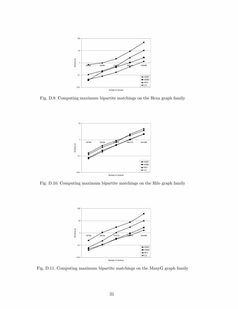
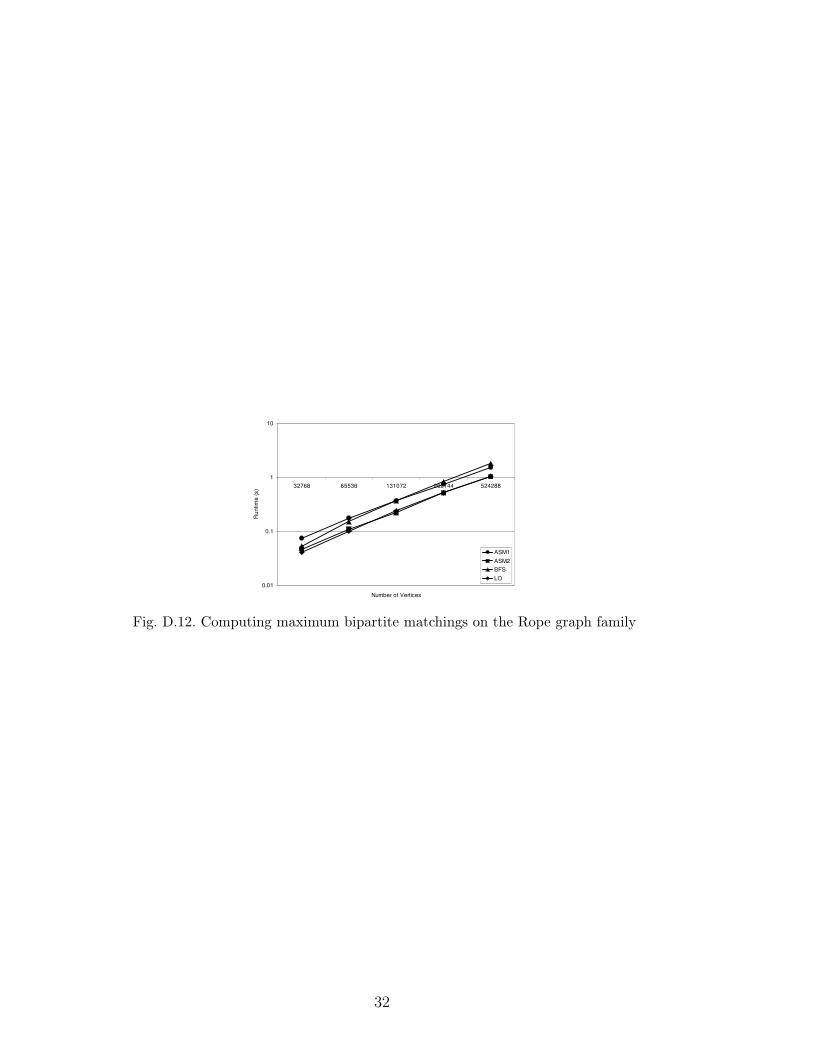
Next, we compared ASM1 and ASM2 with two algorithms for computing maxi-mum bipartite matchings from [2]: BFS, their fastest implementation based onaugmenting paths, and LO, their fastest implementation based on the push-relabel method. Table 1(b) summarizes the results of these experiments ongraphs with 219 vertices. Appendix D contains graphs of the experimental re-sults over a wide range of graph sizes. As before, the reported value is themean of the execution time over five graphs with different seeds. These resultsshow that ASM2 is roughly as efficient as LO, the best known algorithm forthe maximum bipartite matching problem, on a variety of input graphs.

1 We acknowledge Andrew Goldberg’s assistance in finding such a transformationwith a linear number of additional vertices and edges.

21

(a)

Graph ASM1 ASM2 CSA LEDA

FewG 1.190 0.165 0.931 22.324

Grid 0.428 0.059 0.975 5.068

Hexa 0.969 0.187 1.531 20.906

Hilo 0.427 0.218 2.059 8.952

ManyG 1.096 0.109 0.897 13.603

Rope 0.175 0.109 0.978 5.890

Zipf 3.962 0.078 — —

Total 8.247 0.925 >7.371 >76.744

(b)

Graph ASM2 BFS LO

FewG 2.696 11.406 1.531

Grid 0.428 3.075 0.850

Hexa 2.715 10.721 1.315

Hilo 2.237 2.247 4.728

ManyG 2.728 10.228 1.631

Rope 1.015 1.818 1.047

Zipf 0.841 0.287 0.693

Total 12.66 39.782 11.795

Table 1(a) gives the execution time in seconds of four algorithms for the optimal semi-matching problem, on a variety of graphs with 65,536 vertices. “—” indicates thatno results could be recorded since the graph exceeded the memory of our test machine.(b) gives the execution time in seconds of three algorithms for the maximum bipartitematching problem, on a variety of graphs with 524,288 vertices.

7 Conclusions and Future Work

This paper has introduced the optimal semi-matching problem for bipartitegraphs. We have seen how this problem can be reduced to known networkoptimization problems, and that solutions to this problem minimize all Lp-norms, including the L∞-norm. We have presented two new algorithms forsolving this problem, ASM1 and ASM2; the former has a good worst-case timebound, and the latter performs very well in practice. ASM2 also solves themaximum bipartite matching problem with roughly the same efficiency as the

22

best known algorithms.

We feel that our analysis of ASM2 is not the best possible. As future work, weplan to investigate improved bounds for this algorithm. Other future work mayinclude a generalization of the semi-matching problem to allow weighted edgesin the graph. As in the unweighted case, one can adopt network optimizationalgorithms to compute optimal weighted semi-matchings; thus, the challengeis in developing algorithms for the weighted problem with similar efficiency toour current algorithms for the unweighted problem.

References

[1] R. K. Ahuja, T. L. Magnanti, J. B. Orlin, Network Flows: Theory, Algorithms,and Applications, Prentice Hall, 1993.

[2] B. V. Cherkassky, A. V. Goldberg, P. Martin, J. C. Setubal, J. Stolfi, Augmentor push: a computational study of bipartite matching and unit-capacity flowalgorithms, ACM J. Exp. Algorithmics 3 (8),Source code available at http://www.avglab.com/andrew/soft.html.

[3] J. Hopcroft, R. Karp, An n5/2 algorithm for maximum matchings in bipartitegraphs, SIAM J. Computing 2 (1973) 225–231.

[4] H. W. Kuhn, The Hungarian method for the assignment problem, Naval Res.Logist. Quart. 2 (1955) 83–97.

[5] E. Lawler, Combinatorial Optimization: Networks and Matroids, Dover, 2001.

[6] Y. Azar, On-line Load Balancing, in: A. Fiat, G. Woeginger (Eds.), OnlineAlgorithms: The State of the Art (LNCS 1442), Springer-Verlag, 1998, Ch. 8.

[7] Active Directory,http://www.microsoft.com/windowsserver2003/technologies.

[8] W. A. Horn, Minimizing average flow time with parallel machines, OperationsResearch 21 (1973) 846–847.

[9] T. H. Cormen, C. E. Leiserson, R. L. Rivest, C. Stein, Introduction toAlgorithms, 2nd Edition, MIT Press, 2001.

[10] R. L. Graham, E. L. Lawler, J. K. Lenstra, A. H. G. Rinnooy Kan, Optimizationand approximation in deterministic sequencing and scheduling: A survey, Ann.Discrete Math 5 (1979) 287–326.

[11] J. L. Bruno, E. G. Coffman, R. Sethi, Scheduling independent tasks to reducemean finishing time, Communications of the ACM 17 (1974) 382–387.

[12] B. Awerbuch, Y. Azar, E. Grove, M. Y. Kao, P. Krishnan, J. S. Vitter,Load Balancing in the Lp Norm, in: Proceedings of the IEEE Symposium onFoundations of Computer Science, 1995.

23

[13] Y. Azar, A. Z. Broder, A. R. Karlin, On-line load balancing, TheoreticalComputer Science 130 (1) (1994) 73–84.

[14] Y. Azar, J. Naor, R. Rom, The Competitiveness of On-line Assignments, in:Proceedings of the ACM-SIAM Symposium on Discrete Algorithms, 1992.

[15] D. Abraham, Algorithmics of two-sided matching problems, Master’s thesis,Department of Computing Science, University of Glasgow (2003).

[16] W. Rudin, Principles of Mathematical Analysis, 3rd Edition, McGraw-Hill,1976.

[17] A. Goldberg, R. Kennedy, An efficient cost scaling algorithm for the assignmentproblem, Math. Prog. 71 (1995) 153–178,Source code available at http://www.avglab.com/andrew/soft.html.

[18] K. Melhorn, S. Naher, LEDA: A Platform for Combinatorial and GeometricComputing, Cambridge University Press, 1999.

24

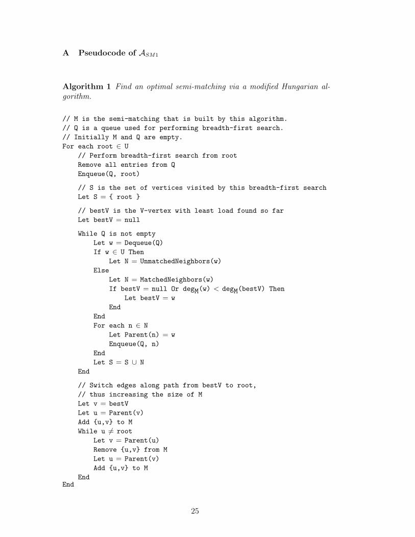
A Pseudocode of ASM1

Algorithm 1 Find an optimal semi-matching via a modified Hungarian al-

gorithm.

// M is the semi-matching that is built by this algorithm.

// Q is a queue used for performing breadth-first search.

// Initially M and Q are empty.

For each root ∈ U

// Perform breadth-first search from root

Remove all entries from Q

Enqueue(Q, root)

// S is the set of vertices visited by this breadth-first search

Let S = root

// bestV is the V-vertex with least load found so far

Let bestV = null

While Q is not empty

Let w = Dequeue(Q)

If w ∈ U Then

Let N = UnmatchedNeighbors(w)

Else

Let N = MatchedNeighbors(w)

If bestV = null Or degM(w) < degM(bestV) Then

Let bestV = w

End

End

For each n ∈ N

Let Parent(n) = w

Enqueue(Q, n)

End

Let S = S ∪ N

End

// Switch edges along path from bestV to root,

// thus increasing the size of M

Let v = bestV

Let u = Parent(v)

Add u,v to M

While u 6= root

Let v = Parent(u)

Remove u,v from M

Let u = Parent(v)

Add u,v to M

EndEnd

25

In this pseudocode, MatchedNeighbors(w) returns a set containing all neigh-bors of vertex w that are matched with vertex w. Similarly, UnmatchedNeighbors(w)returns all neighbors of vertex w that are not matched with vertex w.

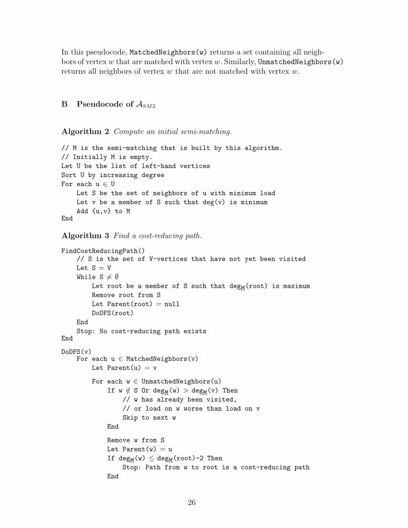
B Pseudocode of ASM2

Algorithm 2 Compute an initial semi-matching.

// M is the semi-matching that is built by this algorithm.

// Initially M is empty.

Let U be the list of left-hand vertices

Sort U by increasing degree

For each u ∈ U

Let S be the set of neighbors of u with minimum load

Let v be a member of S such that deg(v) is minimum

Add u,v to MEnd

Algorithm 3 Find a cost-reducing path.

FindCostReducingPath()// S is the set of V-vertices that have not yet been visited

Let S = V

While S 6= ∅Let root be a member of S such that degM(root) is maximum

Remove root from S

Let Parent(root) = null

DoDFS(root)

End

Stop: No cost-reducing path existsEnd

DoDFS(v)For each u ∈ MatchedNeighbors(v)

Let Parent(u) = v

For each w ∈ UnmatchedNeighbors(u)

If w /∈ S Or degM(w) > degM(v) Then

// w has already been visited,

// or load on w worse than load on v

Skip to next w

End

Remove w from S

Let Parent(w) = u

If degM(w) ≤ degM(root)-2 Then

Stop: Path from w to root is a cost-reducing path

End

26

DoDFS(w)

End

EndEnd

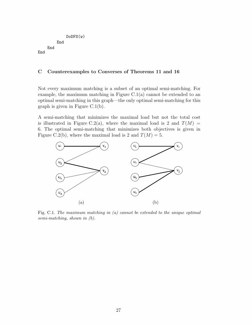
C Counterexamples to Converses of Theorems 11 and 16

Not every maximum matching is a subset of an optimal semi-matching. Forexample, the maximum matching in Figure C.1(a) cannot be extended to anoptimal semi-matching in this graph—the only optimal semi-matching for thisgraph is given in Figure C.1(b).

A semi-matching that minimizes the maximal load but not the total costis illustrated in Figure C.2(a), where the maximal load is 2 and T (M) =6. The optimal semi-matching that minimizes both objectives is given inFigure C.2(b), where the maximal load is 2 and T (M) = 5.

!"

!

!$#

!&%

(a)

')(

'*

+(

+ *

+,

+$-

(b)

Fig. C.1. The maximum matching in (a) cannot be extended to the unique optimalsemi-matching, shown in (b).

27

./0"/

0$1

0$2

0&3

.1

. 2

(a)

456"5

6$7

68

6&9

47

4 8

(b)

Fig. C.2. (a) shows a semi-matching that is optimal with respect to the L∞ normof the load on the right-hand vertices. (b) shows the unique semi-matching thatis optimal with respect to both the L∞-norm and the L2-norm of the load on theright-hand vertices.

D Experimental Results

0.01

0.1

1

10

100

32768 65536 131072 262144 524288

Number of Vertices

Run

time

(s)

ASM1ASM2CSALEDA

Fig. D.1. Computing optimal semi-matchings on the FewG graph family

0.01

0.1

1

10

32768 65536 131072 262144 524288

Number of Vertices

Run

time

(s)

ASM1

ASM2

CSA

LEDA

Fig. D.2. Computing optimal semi-matchings on the Grid graph family

28

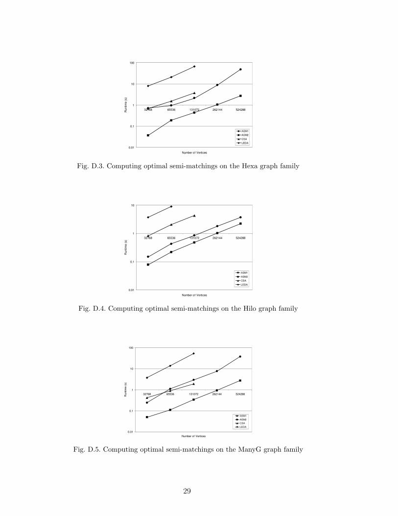
0.01

0.1

1

10

100

32768 65536 131072 262144 524288

Number of Vertices

Run

time

(s)

ASM1ASM2

CSALEDA

Fig. D.3. Computing optimal semi-matchings on the Hexa graph family

0.01

0.1

1

10

32768 65536 131072 262144 524288

Number of Vertices

Run

time

(s)

ASM1

ASM2CSA

LEDA

Fig. D.4. Computing optimal semi-matchings on the Hilo graph family

0.01

0.1

1

10

100

32768 65536 131072 262144 524288

Number of Vertices

Run

time

(s)

ASM1ASM2CSALEDA

Fig. D.5. Computing optimal semi-matchings on the ManyG graph family

29

0.01

0.1

1

10

32768 65536 131072 262144 524288

Number of Vertices

Run

time

(s)

ASM1

ASM2

CSA

LEDA

Fig. D.6. Computing optimal semi-matchings on the Rope graph family

0.01

0.1

1

10

100

32768 65536 131072 262144 524288

Number of Vertices

Run

time

(s)

ASM1

ASM2BFS

LO

Fig. D.7. Computing maximum bipartite matchings on the FewG graph family

0.01

0.1

1

10

32768 65536 131072 262144 524288

Number of Vertices

Run

time

(s)

ASM1

ASM2

BFS

LO

Fig. D.8. Computing maximum bipartite matchings on the Grid graph family

30

0.01

0.1

1

10

100

32768 65536 131072 262144 524288

Number of Vertices

Run

time

(s)

ASM1ASM2

BFSLO

Fig. D.9. Computing maximum bipartite matchings on the Hexa graph family

0.01

0.1

1

10

32768 65536 131072 262144 524288

Number of Vertices

Run

time

(s)

ASM1

ASM2

BFS

LO

Fig. D.10. Computing maximum bipartite matchings on the Hilo graph family

0.01

0.1

1

10

100

32768 65536 131072 262144 524288

Number of Vertices

Run

time

(s)

ASM1

ASM2

BFS

LO

Fig. D.11. Computing maximum bipartite matchings on the ManyG graph family

31

0.01

0.1

1

10

32768 65536 131072 262144 524288

Number of Vertices

Run

time

(s)

ASM1ASM2BFSLO

Fig. D.12. Computing maximum bipartite matchings on the Rope graph family

32