SEMI-MAJOR AXIS KNOWLEDGE AND GPS ORBIT DETERMINATION

J. Russell Carpenter" and Emil R. Schiesser *

In recent years spacecraft designers have increasingly sought to use onboard Global Po-

sitioning System receivers for orbit determination. The superb positioning accuracy of

GPS has tended to focus more attention on the system's capability to determine the

spacecraft's location at a particular epoch than on accurate orbit determination, per se.

The determination of orbit plane orientation and orbit shape to acceptable levels is less

challenging than the determination of orbital period or semi-major axis. It is necessary to

address semi-major axis mission requirements and the GPS receiver capability for orbital

maneuver targeting and other operations that require trajectory prediction. Failure to de-

termine semi-major axis accurately can result in a solution that may not be usable for tar-

geting the execution of orbit adjustment and rendezvous maneuvers. Simple formulas,

charts, and rules of thumb relating position, velocity, and semi-major axis are useful in

design and analysis of GPS receivers for near circular orbit operations, including rendez-

vous and formation flying missions. Space Shuttle flights of a number of different GPS

receivers, including a mix of unfiltered and filtered solution data and Standard and Pre-

cise Positioning Service modes, have been accomplished. These results indicate that

semi-major axis is often not determined very accurately, due to a poor velocity solution

and a lack of proper filtering to provide good radial and speed error correlation.

Aerospace Engineer, Guidance, Navigation, and Control Center, Code 572, NASA Goddard Space Flight Center, Greenbelt, MI_0771.

Specialist Engineering.The Boeing Company Space and Det_nse Systems - Houston Division, Houston, TX 77058

1

https://ntrs.nasa.gov/search.jsp?R=20000084327 2018-09-02T15:32:59+00:00Z

INTRODUCTION

For most people t'amiliar with celestial mechanics, the Keplerian elements are among the most

intuitive of the various sets used to describe orbital motion. However, in the modern era, orbit

determination has mostly been accomplished using Cartesian coordinates. Cartesian parameters

in recent years are also used in Global Positioning System (GPS) orbit determination. GPS re-

ceivers have the ability to determine accurate instantaneous position, and in some cases ade-

quately accurate instantaneous velocity, but the determination of a state vector useful for state

prediction, maneuver planning, etc., is another matter.

Orbital state determination and prediction accuracy depends on, among other factors, the error in

force models used rather than on the size of the forces affecting spacecraft motion. For near-

circular orbits, the error in state prediction is due chiefly to initial orbital period or semi-major

axis error, and imperfect force models used in prediction. The contributions from spacecraft

venting, uncoupled attitude control thrusting, atmospheric drag, and solar radiation pressure

force model errors are dependent on the type of vehicle, orbital characteristics, and the prediction

interval. For some orbital applications in which gravitational field error is of prime interest, it is

necessary to consider the effect of tides.

The accuracy with which orbital period can be determined depends on measurement type and

geometry, and the error associated with force models used in the navigation process. Traditional

satellite orbit determination uses measurements, such as range and Doppler, from ground track-

ing stations or tracking and data relay satellites. It is necessary to use data spread over relatively

long arcs (3/4 to several revolutions) from these sources to accurately determine the orbit since

2

themeasurementsarenotcontinuousandrelateto only a portion of the state at a time. GPS pro-

vides continuous measurements that relate to all components of the state at a time so that, if de-

sired, accurate local instantaneous position and velocity may be determined with a low order

gravitational field model and a filter with a short memory. Such a solution might not provide

accurate orbit state prediction since only a small portion of the orbit is measured. The accuracy

may be improved through the use of a high-order gravitational field for both state determination

and prediction, or as for traditional processes, a low order field but with a much longer filter

memory.

Despite these complications, relatively simple means were developed, at least as far back as the

1960s, for the assessment of state prediction error due to initial state vector error and the effect of

unmodeled forces. The intent of this paper is to expose long-standing back-of-the-envelope

analyses of the orbital period error of an initial state vector, as reflected by semi-major axis error.

The variation (osculation) in semi-major axis due to the non-spherical earth gravitational field is

not relevant to the subject of the paper, assuming that an adequately accurate earth gravitational

field model is used for the chosen navigation process.

Coordination of Position and Velocity

Coordinated position and velocity estimates are required to determine orbit orientation, shape

and period or semi-major axis (SMA). The error in predicted along-track position depends on

the error in orbital period or the error in SMA, as affected by the proper coordination of position

and velocity knowledge. These errors in position and velocity can be considered to be knowl-

edgeerrorsin the current orbit, or maneuver execution errors created in trying to achieve an orbit

change. Kepler discovered that for an ideal orbit, the square of the period is proportional to the

cube of the semi-major axis. Letting Tp denote the period, and a denote the SMA, Kepler's law

may be written I

(1)

where p = GM, the product of the gravitational constant, G, and the planetary mass, M. Eq. (1)

may be used to establish a relationship 2 between a variation in 5a, the nominal SMA, and a

variation in orbital period, 5Tp:

5Tp = 3n f_Sa. (2)

Based on the principle of conservation of energy, the sum of kinetic and potential energy,

-_/(2a), is a constant I in the absence of contact forces, such as drag, vents, or maneuvers. Thus,

SMA knowledge is also an indication of knowledge of the orbit's energy. Letting v denote ve-

locity magnitude and r position magnitude, the energy integral may be written

1 2 v 2- , (3)

a r p

from which the following variational equation is derived:

-_6a =2 6r + 2V Sv.r" ].t

(4)

Eq. (3) is based on the assumption that the earth is spherical and the orbit is a circle or ellipse.

For actual orbits, the ,]2 oblateness term causes variations on the order of a few kilometers

4

throughouta revolutioncomparedto a sphericalEarthorbit. Variation in Earthmassdistribution

beyond the ,/2 Earth flattening results in additional but smaller departures from a conic orbit.

Transt'brrnation from instantaneous "osculating" orbit elements to so-called mean element sets is

often useful. However, this paper is primarily concerned with the analysis of variations in the

osculating semi-major axis, which is derived from the instantaneous position and velocity, and

variational analysis can be performed using Keplerian equations.

Many orbits of practical interest, such as low Earth orbits (LEO) and geosynchronous Earth or-

bits (GEO), are nearly circular. For a circular orbit, a = r, and from Eq. (3) v = (w'r) tr2. With

these assumptions, Eq. (4) simplifies to Eq. (5):

8a = 28r + 2rsv (5)V

It is possible to have an error in radius and an error in speed but no error in SMA. The relation-

ship between the radius and speed error for zero SMA error is shown in Eq. (6), which was ob-

tained by setting 5a to zero in Eq. (5).

,Sr = -rsv. (6)V

For LEO cases, the ratio r/v is on the order of 1000. Thus a one meter per second down-track

velocity perturbation must be balanced by a -1000 meter radial position perturbation if SMA is

to be maintained.

Position and velocity coordination affects flight-path angle in manner similar to that for the

SMA. The flight-path angle, y, is the complement of the angle between the velocity vector, v,

5

and the position vector,r, and canbe visualizedas theanglebetweenthe velocity vector and a

planeperpendicularto theradiusvector:

rvsinT = r.v (7)

The flight path angle is zero for a non-osculating circular orbit, which implies r. v = 0.

It is useful to consider an orthogonal set of perturbations in the radial, along-track, and cross-

track directions, 5rR,Srs,Sr c, and their time derivatives, denoted by 5vR,Svl,Sv c . Figure 1 il-

lustrates the radial, along-track, and cross-track perturbations.

v 1_ v + 5v

]=_×i _.\\ i=r/r

r /(__r ,'Orbital_.-1 Earth " Path

5r = SrRi+ Srli + Srcf_

k=r×v/Jr×vI v=Sv i+Svsi+Svcf,

Fi_ure 1: Radial, alon_-track, and cross-track perturbations.

In terms of the notation used above, 5r R z 5r, and for near-circular orbits, velocity deviation is

nearly all along-track, so that 5vz -_ 5v. In terms of these perturbations, a relationship between

deviations in along-track position, 5rz, and radial rate, 5v R , for zero flight path angle may be

derived:

0=r.v

[Sv ,Sv,,Sv,]+[0,v,0]. ]= rSv R + vSrj

(8)

Eq. (8) reveals that if _, is held to zero to preserve the nominally zero flight-path angle, then a

change in along-track position, 6r_, must be compensated by a change in radial velocity:

V

8s_ = --8_. (9)r

The same rule-of-thumb ratio of approximately 1000 to 1 seen for radial and speed error correla-

tion for zero SMA error shows up again in Eq. (9) for the relationship between along-track posi-

tion and radial rate for zero flight path angle deviation. A one meter per second perturbation to

radial velocity must be balanced by a -1000 meter change in down-track position, if near-zero

flight-path angle is to be maintained.

Effects of Poor Semi-Major Axis Knowledge

Along-track error growth. A semi-major axis error reflects a period error (Eq. (2)) and the satel-

lite will complete more or less than one actual revolution during its nominal period than pre-

dicted. For near-circular orbits, the resulting along-track error is

8r, = -v(t / r. )5"rp, (lo)

where the negative sign convention recognizes that if the actual period is less than nominal, the

satellite ends up farther along in its orbit than nominal, which is taken to be a positive along-

track error. Setting t = Tp in Eq. (10) gives the along-track error per revolution:

5r_ = -v5 Tp, ( 11 )

Substituting Eq. (2) into Eq. (11), and assuming the velocity to be the circular orbit velocity, re-

sults in Eq. (12):

5rz = -3rtSa, (12)

7

which leadsto a commonrule of thumbtbr along-trackerror growth perorbit revolution, i.e. the

alongtrack errorper revolution is equalto minustentimesthesemi-majoraxiserror-'.

Maneuver execution errors. The performance of a proper orbital maneuver is affected by tar-

geting error, which is usually dominated by local SMA error, and imperfect execution of the tar-

geted maneuver. Maneuver execution error may be due to inaccurate measurement of the veloc-

ity change or the duration of the maneuver, depending on execution approach, as well as im-

proper maneuver attitude and an imperfect thrust "tailoff" model. In the case of an instantaneous

or short maneuver, there is no appreciable change to the position error, and any along-track ve-

locity execution error will not be balanced by a corresponding radial position error, and will re-

sult in a semi-major axis error per Eq. (6).

Covariance matrix propagation. A less familiar example occurs in the problem of initializing

the covariance matrix for a sequential orbit determination filter that uses Cartesian coordinates.

Sequential state determination provides a current running estimate, but has the feature that only a

portion of the state is typically observable when using the measurement set available at current

time. The filter retains the history of past measurement processing as an estimate of the uncer-

tainty of the state in the form of a variance/co-variance matrix that must be initialized. The ini-

tial covariance matrix should reflect the uncertainty in the initial state vector. The state and its

uncertainty (in the form of the covariance matrix) have to be propagated for some time before the

first measurement becomes available. As a result, the initial covariance matrix must reflect the

proper uncertainty in SMA and flight path angle. Eqs. (6) and (9) may be used to establish ra-

dial, speed, radial-rate and along-track variances and associated co-variances.

8

Figure2 illustratestheeffectof the initial covariancematrix on propagation. The matrix shown

hasunits ofm and m/sand therowsandcolumnsare rl_,r,,rc,v,_,vl, and v(.. The initial covari-

ance shown on the plot was propagated without process noise, in a circular low Earth orbit

whose period is 5828.5 seconds to produce the figure. The initial value of the SMA uncertainty

(computed using Eq. (16) shown in the next section) is given at the top of each plot. The upper

subplot shows overall error growth when the error in radius matches the error in speed per the

rule of thumb (1000 m radial error per -1 m/s speed error). The lower subplot shows error

x 104 a,,(O) = 873.5304

4Initial Covariance =

' 1000.00

3- 0.o0' 0.00

0.00

in -0.90®2

1

0.00 0.00 0.00 -0.90 0.00 i

3000.00 -0.00 -0.90 0.00 0.00

-0.00 i00.00 0.00 0.00 0.00-0.90 0.00 3.00 0.00 0.00

0.00 0.00 0.00 1.00 0.00

0.00 0.00 0.00 0.00 0.00 1.00

, i--% .................... iO'fl ._

H-.... o,o0 _ _ _ _ _"_ --_ . .-_- ._-_-'- ---:==_-- . ..... .-v--------:r-_-_._............... _. . . , ............. _.....

0 2000 4000 6000 8000 10000 12000

sec

x 104 aa(O) = 1677.5422

4

Initial Covariance =i00. O0 O. O0 O. O0 O. O0 -0.90 0. O0 !

3- 0.00 I00.00 0.00 -0.90 0.00 0.00 .- ---0.00 0.00 i00.00 0.00 0.00 0.00" J

i 0.00 -0.90 0.00 3.00 0.00 0.00

tn I -0.90 0.00 0.00 0.00 1.00 .-_ 0.00

2i[ 0.00 0.00 0.00 0.00 0.00 1.00 A

i l -- " °'rl ! _

i : _'r c i I

O_ _ - .... ..... _._-7:::-_ ...... .-----T-...................... -,--_-,

0 21X)O 4000 6000 8000 10000 12000

sec

Figure 2: Comparison of covariance propagation with matched and unmatched SMA

and flight-path angle relationships

growth for unmatched errors one might expect from some GPS point solutions. The I00 m ra-

dial error (smaller than the 1000 m radial error in the upper matrix) cannot compensate for the

1 m/s speed error and results in along-track error gro_,vxh that is about double that of the matched

case, shown in the upper subplot. Either the 1 m/s error must be reduced to 0.1 m/s or the radial

error must be increased to 1000 m to achieve reduced along-track error growth.

SIMPLE FORMULAS FOR SEMI-MAJOR AXIS UNCERTAINTY

This section illustrates some simple formulas and charts that relate the statistical variance of the

Cartesian states to the semi-major variance. Modification of these formulas for relative naviga-

tion applications is also discussed.

Absolute State Semi-major Axis

For a Cartesian state vector x = [r r, vV], a first order approximation that relates changes in the

state away from a nominal value (denoted by the subscript o) to changes in the SMA is given by

°aI (X-Xo). (13)a -- a o ._ -_ xfxo

For

-:°2FrTYllA(Xo)- --r-- , (14)

where the partial derivative has been evaluated assuming a two-body potential, the error variance

of the SMA in terms of the state error covariance is

10

I:]= -(x,,)= )T

(15)

In deriving Eq. (15), Eqs. (13) and (14) have been used, the symbol "E" denotes the expectation

operator, and Px is the state error covariance matrix. The following simplification of Eq. (15),

valid for near-circular orbits may be found in Reference 2:

+ P 0-2_ =2 er_, +2 p,,.,c, er_, ., . (16)

This equation may also be derived from Eq. (5), using Eqs. 2 and 3.

In Eq. (16), p,,,, denotes the correlation coefficient between radial position error and in-track

velocity error, and g,, and c,, denote the radial position error and in-track velocity error stan-

dard deviations, respectively.

Eq. (16) may be used as a design and analysis aid, especially in graphical form. Also, either

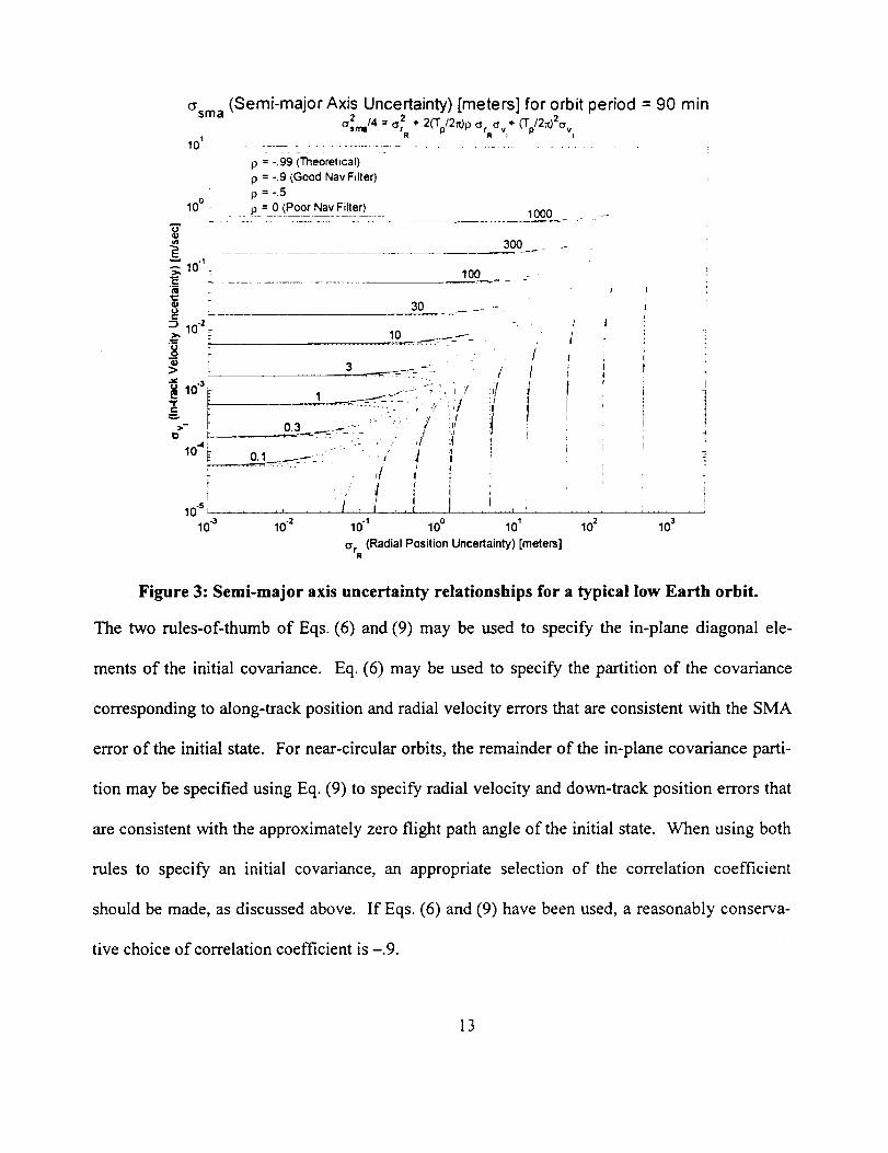
Eq. (15) or Eq. (16) is useful as a "figure of merit" for orbit determination filters. Figure 3

shows one means of graphically representing Eq. (16) for LEO scenarios. Figure 3 depicts sev-

eral families of relationships among the principal contributors to SMA uncertainty for a LEO

mission. Each family of curves illustrates a subset of the range of radial position and along-track

velocity errors that generate the same SMA error, from 0.1 meter to 1000 meters.

Along the main diagonal of the chart, the families split based on the value of the correlation coef-

ficient. The correlation coefficient captures the deterministic relationship implied among the ra-

Il

dial positionanddown-trackvelocity errorsby Eq.(6). To theextent that theseerrorsareprop-

erly coordinated,a given level of knowledgeabouteitheroneimpliessomedegreeof knowledge

about the other. The coefficient is negativebecauseof the negative relationship stated by

Eq.(6). Theregionof theplot in whichthe familiessplit correspondsto a "sweetspot" of proper

coordinationamongpositionandvelocity.

At one extreme, radial position and down-track velocity errors are completely uncorrelated

(p = 0), and the SMA error is bounded below by the lower of its corresponding radial position

and speed errors. For example, no matter how good position knowledge gets, SMA knowledge

will be no better than about 100 meters if speed knowledge cannot be improved beyond about

0.05 meters per second. However, if radial position and speed errors are properly coordinated

(via Eq. (6)), the SMA knowledge can be dramatically improved, because a corresponding in-

crease in the correlation among radial position and down-track velocity errors is possible. For

example, using the "1000 to 1" rule of Eq. (6), a radial position error of 100 meters should corre-

spond to a down-track velocity error of about -. 1 meters per second. As Figure 3 shows, this

combination could correspond to an SMA error of about 100 meters if the correlation coefficient

is -.9, but would only correspond to an SMA error of just under 300 meters if the correlation co-

efficient is near zero. A coefficient near the value one would expect if Eq. (6) were nearly ex-

actly satisfied (- -0.99) would give an SMA error on the order of 30 meters. In the limit, the

coefficient reaches -1, the horizontal and vertical branches on the plot disappear, the random

variables become simple deterministic variables, and the linear relationship of Eq. (6) is depicted

as a straight line from lower left to upper right.

12

t--

t_

_8>

C_sma (Semi-major Axis Uncertainty) [meters] for orbit period = 90 min

2 + 2('Tp/2_p ('T'p/2.-,.)2av,Cr2rm/4 = °rR °'rR°'v=+

101

p = -.99 i_eoretlcal) -

p = -9 (Good Nay Filter)

p=-.5

100 - ____ __= 0_!_Poo_[rNav_Filt_e_r) ..... 1000

10 "1100

300__

30 _._-

102 : 10.... -d:7-"_- -

r"

lo" ,!_..._..._:__--. -:- ,_" Y i'"It" , ': !f.- != E ilt _/:,,- , 0.3 ___ "- _: '_:

u ,-- ..... - _- ii i

Io" o.! :..T:_::_:::-- / i _ 'r/ P _ ;

,{' iI !

lo _' , :1',_ ,' ...... I ........ :,10.3 10.2 10"1 100 101

arrR (Radial Position

:/

Uncertainty) [meters]

J

l

10 2 10 3

Figure 3: Semi-major axis uncertainty relationships for a typical low Earth orbit.

The two rules-of-thumb of Eqs. (6) and (9) may be used to specify the in-plane diagonal ele-

ments of the initial covariance. Eq. (6) may be used to specify the partition of the covariance

corresponding to along-track position and radial velocity errors that are consistent with the SMA

error of the initial state. For near-circular orbits, the remainder of the in-plane covariance patti-

tion may be specified using Eq. (9) to specify radial velocity and down-track position errors that

are consistent with the approximately zero flight path angle of the initial state. When using both

rules to specify an initial covariance, an appropriate selection of the correlation coefficient

should be made, as discussed above. If Eqs. (6) and (9) have been used, a reasonably conserva-

tive choice of correlation coefficient is -.9.

13

RelativeStateSemi-major Axis

RelativeSMA, i.e. thedifferencein SMA betweenpairsof vehicles,is of interestfor rendezvous

and formation flying missions. During rendezvous,a "chaser" will executemaneuversto ap-

proachtargetspacecraft.DenotingthechaserSMA by ac, and the target SMA by at, the relative

SMA is

a_l = a _ -a, . (17)

Since ac is a function of the chaser state xc and at is a function of the target state xt, in deriving

the uncertainty of the relative SMA it is useful to define a state consisting of both the chaser and

target states: x r= [xc "r xtV]. Then, as in Eq. (13), a perturbation in the nominal relative SMA may

be approximated by

Oa,_ (x_xo)"an/-ant" _" OX x_xo

(18)

Using the notation of Eq. (14), the partial derivative is evaluated as follows:

LP J L,, JJl,=,.A(xo)=[A_(xo),-A,(xo)]

(19)

The covariance of the chaser�target state, Ix, may be partitioned into chaser-only and target-only

covariances (Pc and Pt), and their cross-covariance matrices (,oct):

(2O)

Using Eqs. (19) and (20) in Eq. (15) results in the following:

14

{_ &lr ,= [.4.(x ,).- .4,(x ,) _ jL.-l,(x,,),-A,(x,,)]"

=.4_.._,.?-,-._,_A,"- A_p.,A,"-(A.p,_,')T

(21)

FLIGHT PERFORMANCE SURVEY

A number of different GPS receivers have been flown on Space Shuttle Orbiter flights, including

a mix of GPS units, some which filtered measurement data and some which extracted the state

deterministically from the data. Some of the GPS units operated in Standard Positioning Service

and others in Precise Positioning Service modes. Both absolute state and relative state perform-

ance have been evaluated. Particular interest has been given to the semi-major axis performance

of the GPS receivers and any associated filtering algorithms, to determine if the GPS has the po-

tential to replace or augment rendezvous navigation sensors.

Absolute State Flight Performance

Twenty-one sets of absolute-state flight data results are shown in Table 1, and in Figure 4, the

flight data are overlaid on a copy of Figure 3. The data used in constructing these tables was ex-

tracted from Refs. 3-6, and from various internal documents. In some cases, either velocity or

SMA data were not available. In general, the flight data indicate that semi-major axis is oi_en

not determined very accurately, typically due to a poor velocity solution and/or a lack of proper

filtering to provide good radial and speed error correlation. Note that the flight data are all from

LEO missions, and have periods varying by a few minutes from the nominal period of

90 minutes used to construct the figure.

Nearly all the flight data lie above the diagonal region in Figure 4 previously described as the

15

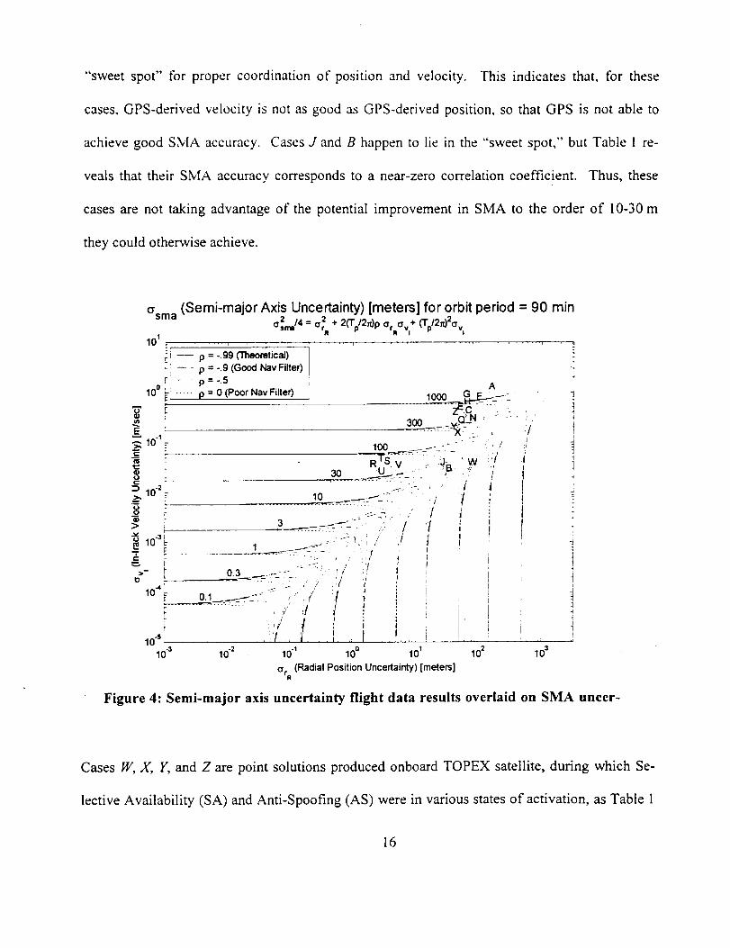
"'sweetspot" tbr proper coordination of position and velocity. This indicates that, for these

cases, GPS-derived velocity is not as good as GPS-derived position, so that GPS is not able to

achieve good SMA accuracy. Cases J and B happen to lie in the "sweet spot," but Table 1 re-

veals that their SMA accuracy corresponds to a near-zero correlation coefficient. Thus, these

cases are not taking advantage of the potential improvement in SMA to the order of 10-30 m

they could otherwise achieve.

Csm a (Semi-major Axis Uncertainty) [meters] for orbit period = 90 mino'2 14 = 2 + (Tp/2_)2O.vlll, mla O'rR 2(Tp/2._p O'rnCtVl ÷

101 :

-- p = -.99 (Theoretical)

-- - p = -.9 (Good Nav Filter)

F - p=-.5

10° _-i ..... P = 0 (Poor Nav Filter)

E

_ 10 "1 =

U

c -2 __ 10

8 ;

> i

c

_,., F I

J l

_ ', ,/_ ,,/ ! l

10"sl ';'[,.......... I10 .3 10 .2 10 "I 10 0

A

100 _ ---" ' / :_

30..... _:-._ - /

_--"--------.- "

'J

;

!

i

L

IIt

i

I,L .... I .... i ,

102 10 s101

ar_ (Radial Position Uncertainty) [meters]

Figure 4: Semi-major axis uncertainty flight data results overlaid on SMA uncer-

Cases W, X, II, and Z are point solutions produced onboard TOPEX satellite, during which Se-

lective Availability (SA) and Anti-Spoofing (AS) were in various states of activation, as Table 1

16

describes.Although TOPEX's 112minuteperiod is approximately25% longer than the nominal

periodusedto produceFigures3 and4, its SMA is only 13% larger,an error which is not sig-

nificant on the logarithmic scale the figures use. With this caveatin mind, it appearsthat the

SA/AS-free case,CaseW, actually has a velocity that is good enough to produce an SMA error

on the order of 30 m. However, its position solutions are not quite accurate enough, nor perhaps

is its correlation of position and velocity, as Table 1 indicates its SMA error due be over 100 m.

To establish performance, flight data were compared to best estimated trajectories (BETs), gen-

erated with various procedures. Most of the BET procedures have been verified to be accurate to

about 30 meters RMS in position and a few hundredths of a meter per second RaMS in velocity 7.

The Post-flight Attitude and Trajectory History (PATH) BET is probably less accurate in posi-

tion, but more accurate in velocity, than the Wide Area Differential GPS (WADGPS) BET. (The

PATH accuracy is specified to be on the order of 200 meters in position and 0.2 m/s in velocity

RaMS in the worst axis, but it is generally believed to be much better.) In some cases, filtered

position data from an independent, PPS-capable GPS receiver was used as the BET. These

BETs are believed to be slightly more accurate in position than the WADGPS BET is, and com-

parable to the PATH BET in velocity. The SLR+DORIS BETs used for the TOPEX data are

accurate to a few cm in position, and a few tenths of a mm/sec in velocity.

17

°

E_

_×>

_ 0__"0__z _ __

_._

_, i__e_ gg4_- __N

O0

_8

_00000

000

000000

0000_

_ _-_.-

:_ _

ffl C_ (0 u'I _ uJ

Relative State Flight Performance

NASA has jointly performed two relative GPS (RGPS) navigation flight experiments with the

European Space Agency (ESA) 3"6. During these experiments, a near-realtime relative GPS Kal-

man filter processed pseudorange data from GPS receivers aboard the Space Shuttle and a free

flying satellite deployed and retrieved by the Shuttle. This filter was designed to estimate com-

mon biases affecting GPS receivers aboard two co-orbiting spacecraft tracking the same GPS

satellites, and was expected to approach pseudorange (not carrier phase) differential type per-

formance when measurements from at least four common satellites were processed. Recently,

both ESA and the National Space Development Agency of Japan have performed further relative

GPS experiments s'9. STS-80 data have also been processed at the University of Colorado at

Boulder (CU) l°. Table 2 summarizes relative state performance from the various RGPS experi-

ments.

The RGPS results may be compared with Table 3, which shows typical performance of the ex-

isting Shuttle rendezvous navigation system. The existing system consists of a rendezvous radar

Table 3

PERFORMANCE OF EXISTING SHUTTLE RENDEZVOUS SYSTEM

Position (m) Velocity (m/s) I SMA (m)

RadialI Io-,rackIx-trackI RSS aadiaJ[In-trackIX-trackI RSSI151 I 3.6 I 17 I 15.6 0.023 I 0.015 [0008 I 0.029 J 49.4

that provides range, range-rate, azimuth and elevation measurements to an extended Kalman fil-

ter that also utilizes acceleration data from an inertial measurement unit. The data were derived

by comparison of the downlinked Shuttle relative navigation data to a laser-based BET produced

after the flight. Although the relative GPS position accuracy shown in Table 2 is somewhat bet-20

ter than the relative position accuracy of the Shuttle's existing system shown in Table 3, the

GPS-based relative SMA is more than twice as inaccurate. The performance difference is pri-

marily due to poorer relative velocity estimates from the RGPS filter, but also due to poorer cor-

relation among position and velocity errors.

Another approach to GPS relative navigation is to directly difference the solutions from two GPS

Table 4

STATE VECTOR DIFFERENCING PERFORMANCE FROM STS-80

I Sol I Measure- [ Position(m) I Velocity (m/s) I SMA (m_lDet/Filt J ment Radial [ In-track I X-track J RSS Radial JIn-trackJX-track J RSS

d,a I C/A,C/AI 13S.0I 51.7 I ST.0 I lS8.1 I 1.6geI 0._9 I 0.SS0I 2.0221170001

receivers, rather than process the measurement data from both receivers in a single Kalman filter

as described above. Such an approach is obviously much simpler, but does not necessarily re-

move the common error sources. As Table 4 shows, the state vector differencing performance

data from STS-80 show significantly worse performance than the filtered results Table 2 pres-

ents.

However, if the receivers can be operated under the Precise Positioning Service (PPS), with dual-

frequency P/Y-code measurements, most errors larger than a few meters are removed. Under

such circumstances, it could be feasible to perform GPS relative navigation using state vector

differencing. Absolute state flight performance was used to predict relative state accuracy for a

variety of GPS receiver combinations with deterministic vs. filtered solutions based on C/A and

P/Y-code measurements (Table 5). The values in Table 5 were obtained by computing the root

sum squares of the overall absolute state performance summarized at the bottom of Table 1, as-

21

Table 5

STATE VECTOR DIFFERENCING PERFORMANCE SURVEY

+o,iM.e++-I Po,,,+oo+)I ve,o+++)I+M ,m,Oet/Fili + ment Radial l In'track I X-track I RSS Radial I In'track I X-track ] RSS ........

d d_........C/A .C/A,-.92.!.., " 6._0=0...._67=0+.... I_.2-.8_7......I:055.......q.7-0_3....._0.__703....._!.45_O0_,_1445:3. _d,f..... CIA, CIA_.....83.7 . 52.2 ....._5.9:1.....I_115.0 0.872 0.582 0.589 1.203 1076.0

....a,.f..........c]__A,_y_.,652+., 42.s, 4L.5+,._9_-.--6-_i-.-_-6_-_8--l-_-8_-_[i-I-0_1_)_-62_1311.. f, f ..... _C/.A,C/A ........ 74_.3....... 43..0..... 49:8 ..... _99:3...... _0.63_9...... 0:4.29 0.___8.... 0..891 47_.5.9_ f,f .......... C!A,Y ..... _57.7 ...... 30=6......... 35.3 ...... 7_0A_ _ _0.453_...... 0..305.. 0.3!7_+ . _0.631.... 340.3

f, f Y, Y 4.6 3.8 3.0 6.7 0.039 0.041 0.024 0.061 71.5

suming that the errors in the two receivers are uncorrelated (i.e. P_t = 0). The results for absolute

states computed deterministically by the receivers, and absolute states resulting from onboard

orbit determination filters are denoted "d" and "f," respectively, in the first column. The as-

sumption of uncorrelated errors is conservative, corresponding to the case in which the receivers

are tracking zero common satellites. However, only the case in which all satellites tracked are

common will reflect substantially better accuracy.

Although filtering the data helps significantly, state vector differencing, even if one of the two

receivers is P/Y-code capable, is not competitive with either the RGPS filtering approach or the

existing Shuttle rendezvous system capabilities (viz. Tables 2 and 3). Relative state accuracy,

obtained by differencing two absolute states from GPS receivers which filter P/Y-code data,

(shown in the last row of Table 5) was more accurate than RGPS filtered C/A code performance

(Table 2), and comparable to existing Shuttle rendezvous performance (Table 3). There are no

known flight results from an RGPS-type filter using P/Y-code measurements.

None of the flight data results presented utilize carrier phase data, which is commonly used in

static surveying applications to achieve centimeter-level relative positioning. Carrier phase

22

measurementsareanalogousto a veryaccuratepseudo-rangemeasurement,if the measurement

is obtainedasan accumulationof phase,or equivalently range,change. Basedon Figure 3, it

would appearthat even if position were known to better than 1centimeter,SMA knowledge

could not be improvedover existing levelsof performanceunlessboth velocity knowledgewere

obtainedto the0.1to 1mm/seclevel,andpropercorrelationbetweenpositionandvelocity errors

wereachieved.

CONCLUSION

Semi-majoraxisaccuracyaffectsorbital targetingandother functionsdependenton statepropa-

gation and prediction. On-orbit GPSabsoluteand relative SMA Shuttle flight performancere-

suitsachievedto date,thoughpromising,haveoften beenlessthandesirableand at worst inade-

quate. The lack of goodsemi-majoraxis knowledgeis primarily dueto a poor velocity solution

anda lack of proper filtering to providegoodradial and speederror correlation. Use of carrier

phasedatadoesnot appearlikely to improve this situation, unlessit is accompaniedby proper

filtering that is tunedto takeadvantageof orbital dynamics. Sucha filter would createtheneces-

sarystatecorrelationsthat accurateSMA knowledgeimplies. Severalsimpleequations,rulesof

thumb, andchartsconcerningthe semi-majoraxis usedfor back-of-theenvelopeorbit determi-

nationanalysishavebeenpresentedto supportfutureorbital navigationperformanceanalysis. It

is hopedthatthis work will stimulateinnovationsthat will leadto betterorbital GPSorbit deter-

minationperformance.

ACKNOWLEDGEMENTS

Cary Semar of The Boeing Company Space and Defense Systems - Houston Division and the

23

staff and support contractorsof the Flight Designand DynamicsDivision of NASA Johnson

SpaceCenterprovidedmuchof thedatafrom Shuttle flights of the HoneywellEGI and SIGI and

the Litton EGI. Lou Zyla of The Boeing Company Space and Defense Systems - Houston Divi-

sion provided the data from the STS-51 Shuttle GPS experiment. George Davis of Orbital Sci-

ences Corporation provided the TOPEX data.

REFERENCES

1. R. Bate, D. Mueiler, and J. White, Fundamentals of Astrodynamics, Dover, New York, 1971.

2. W. Lear, "Orbital Elements Including the J_ Harmonic," Report No. 86-FM-18/JSC-22213, Rev. I, Mission

Planning and Analysis Division, NASA Johnson Space Center, 9/87.

3. Y. Park, et al., "Flight Test Results from Realtime Relative GPS Flight Experiment on STS-69," Space Flight

Mechanics 199L

4. C. Schroeder, B. Schutz, and P.A.M. Abusali, "STS-69 Relative Positioning GPS Experiment," Space Flight

Mechanics 199L

5. G. Moreau and H. Marcille, "FDI Post-Flight Analysis and Evaluation Report," Matra Marconi Space France

Report No. ARPK-RP-SYS-3744-MMT, 11/8/97.

6. E. Schiesser, et al. "Results of STS-80 Relative GPS Navigation Flight Experiment," Space Flight Mechanics

1998.

7. M. Lisano and R. Carpenter, "High-Accuracy Space Shuttle Reference Trajectories for the STS-77 GPS Atti-

tude and Navigation Experiment (GANE)," Space Flight Mechanics 1997.

8. G. Moreau and H. Marcille, "RGPS Post-flight Analysis of ARP-K Flight Demonstrations," Proceedings of the

ION GPS-98, Nashville, TN, September 1998.

9. I. Kawano, et al., "Result and Evaluation of Autonomous Rendezvous Docking Experiment of ETS-VII," Pro-

ceedings of the AIAA GNC Conference, Portland, OR, August, 1999.

10. D. Highsmith and P. Axelrad, "Relative State Estimation Using GPS Flight Data from Co-orbiting Spacecraft,"

Proceedings of the ION GPS-99, Nashville, TN, September 1999.

24