Sem with amos ii
118
By Hui Bian Office For Faculty Excellence Fall 2011 1
-
Upload
jordan-sitorus -
Category
Business
-
view
318 -
download
3
Transcript of Sem with amos ii

By Hui Bian Office For Faculty Excellence
Fall 2011
1
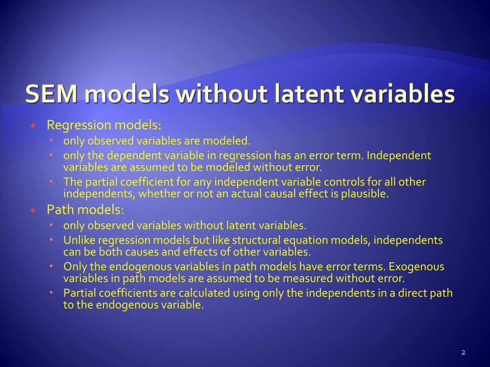
Regression models: only observed variables are modeled. only the dependent variable in regression has an error term. Independent
variables are assumed to be modeled without error. The partial coefficient for any independent variable controls for all other
independents, whether or not an actual causal effect is plausible. Path models:
only observed variables without latent variables. Unlike regression models but like structural equation models, independents
can be both causes and effects of other variables. Only the endogenous variables in path models have error terms. Exogenous
variables in path models are assumed to be measured without error. Partial coefficients are calculated using only the independents in a direct path
to the endogenous variable.
2

AMOS output Standardized regression weights: Structural or path coefficients in SEM. Standardized
estimates are used, for instance, when comparing direct effects on a given endogenous variable in a single-group study.
Indicator variable regression weights. By convention, the indicator variables should have standardized regression weights of .7 or higher on the latent variable they represent.
3

AMOS output: Communalities. The Squared Multiple Correlation is the communality estimate for
an indicator variable. The communality measures the percent of variance in a given indicator variable explained by its latent variable (factor) and may be interpreted as the reliability of the indicator.
If a variable has low theoretic importance and a low communality, it may be targeted for removal in the model-modification.
The communality is equal to the squared standardized regression weight. This is why communalities are sometimes defined as the squared factor loadings, where loadings are defined as the standardized regression weights.
4

AMOS output Unstandardized regression weights: are based on raw
data or covariance matrixes. When comparing across groups (across samples) and
groups have different variances, unstandardized comparisons are preferred.
5

AMOS output The critical ratio and significance of path coefficients.
When the critical ratio (CR) is > 1.96 for a regression weight, that path is significant at the .05 level or better (that is, its estimated path parameter is significant). In the p-value column, three asterisks (***) indicate significance smaller than .001.
The critical ratio and the significance of factor covariances. The significance of estimated covariances among the latent variables are assessed in the same manner: if CR > 1.96, the factor covariance is significant.
6

Purpose of this exercise is to show you how AMOS estimates parameters in multiple regression.
Data used is from Schumacker and Lomax (2004).
We have three predictors and one dependent variable.
7

8
Path diagram
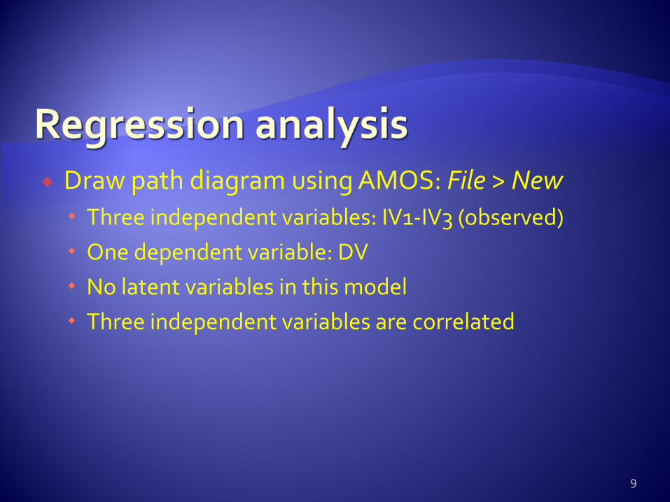
Draw path diagram using AMOS: File > New Three independent variables: IV1-IV3 (observed) One dependent variable: DV No latent variables in this model Three independent variables are correlated
9

The single-headed arrows represent linear dependencies. For example, the arrow leading from IV1 to DV indicates that DV scores depend, in part, on IV1.
The variable error is enclosed in a circle because it is not directly observed. Error represents much more than random fluctuations in DV scores due to measurement error. 10

Model identification The variance of a variable, and any regression
weights associated with it, depends on the units in which the variable is measured.
Error is an unobserved variable, there is no natural way to specify a measurement unit for it. Assigning an arbitrary value to a regression weight associated with error can be thought of as a way of indirectly choosing a unit of measurement for error. 11
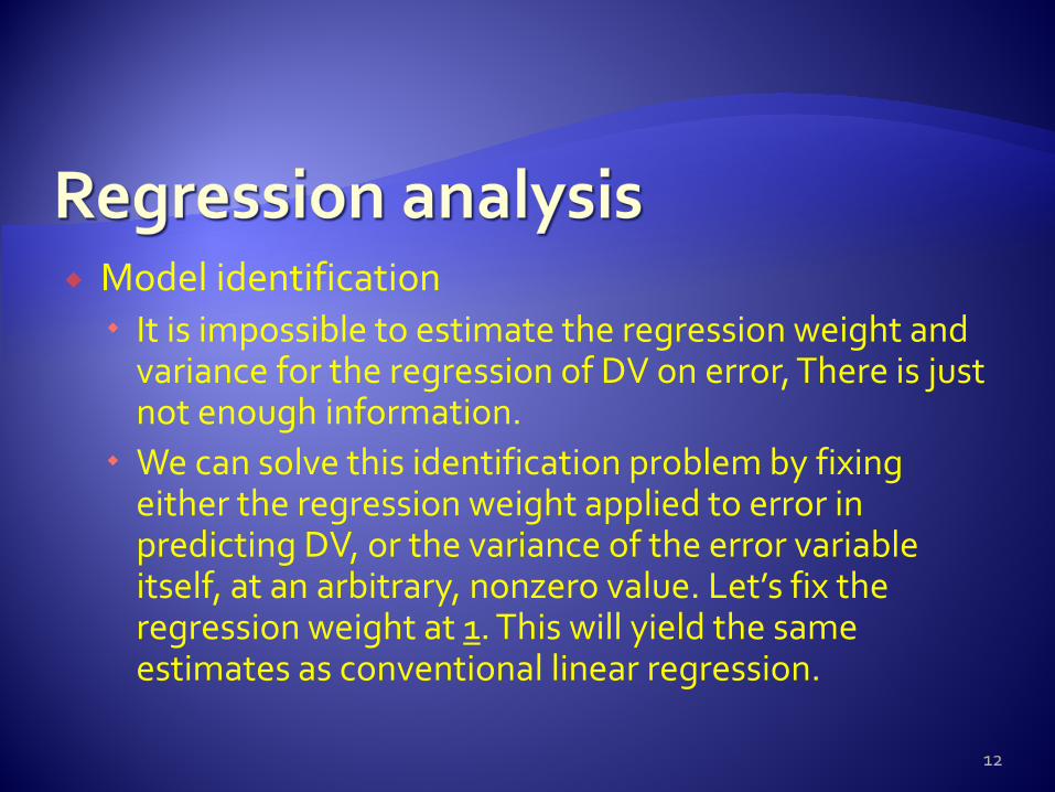
Model identification It is impossible to estimate the regression weight and
variance for the regression of DV on error, There is just not enough information.
We can solve this identification problem by fixing either the regression weight applied to error in predicting DV, or the variance of the error variable itself, at an arbitrary, nonzero value. Let’s fix the regression weight at 1. This will yield the same estimates as conventional linear regression.
12

Model identification Every unobserved variable presents this
identification problem, which must be resolved by imposing some constraint that determines its unit of measurement.
Changing the scale unit of the unobserved error variable does NOT change the overall model fit.
13
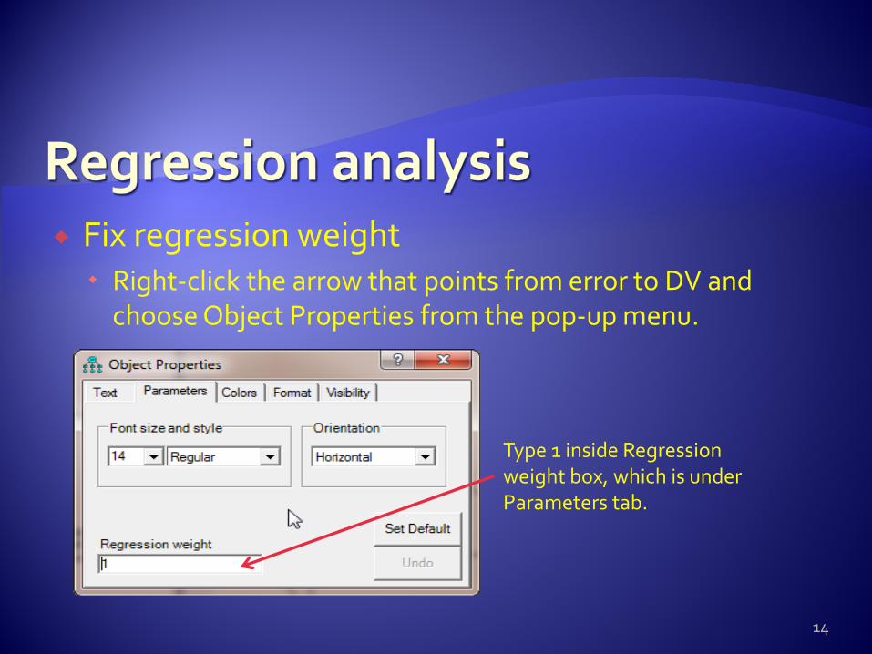
Fix regression weight Right-click the arrow that points from error to DV and
choose Object Properties from the pop-up menu.
14
Type 1 inside Regression weight box, which is under Parameters tab.

Before run data analysis Go to View > Analysis Properties > Click Output tab
15

Text outputs
16

4 sample variances and 6 sample covariances, for a total of 10 sample moments, or use p (p+1)/2, we have 4 observed variables, then the number of sample distinct value is equal to 4(4+1)/2 = 10.
3 regression paths, 4 model variances, and 3 model covariances, for a total of 10 parameters that must be estimated. Hence, the model has zero degrees of freedom.
Such a model is often called saturated or just-identified.
17
Text output
18
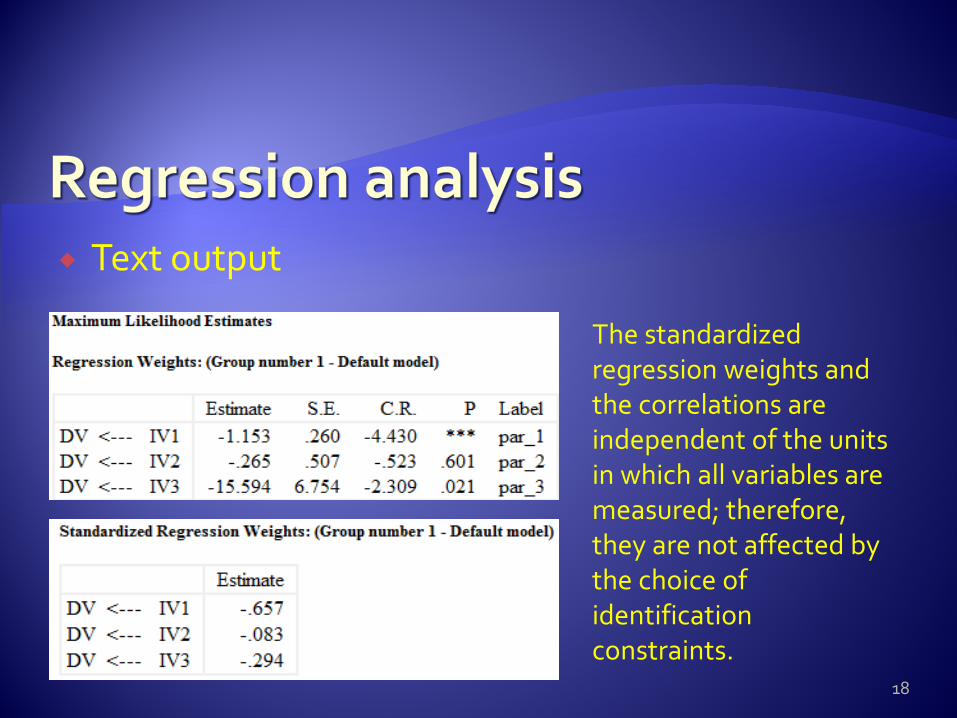
The standardized regression weights and the correlations are independent of the units in which all variables are measured; therefore, they are not affected by the choice of identification constraints.

Text output
19
Squared multiple correlations are independent of units of measurement. Amos displays a squared multiple correlation for each endogenous variable.
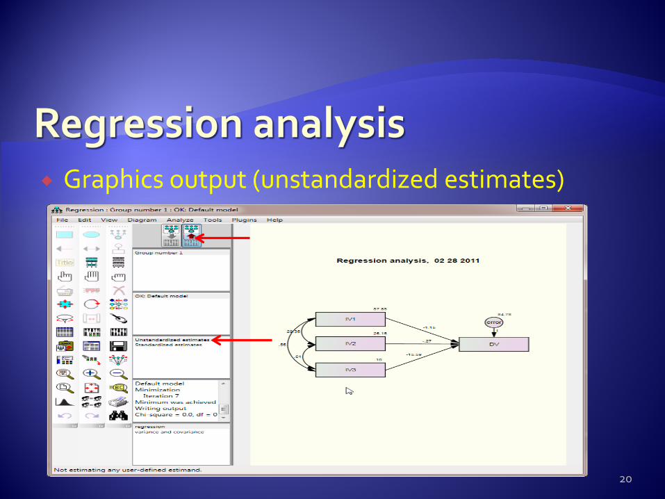
Graphics output (unstandardized estimates)
20

Graphic output (standardized estimates)
21
Correlations

Conclusion In this example, IV1, IV2, and IV3 account for 69% of
the variance of DV. IV1 and IV3 are significant predictors.
22

Path analysis model Only focus on relationships of multiple observed
variables Analysis of several regression equations
simultaneously. Use the same idea of model fitting and testing as any
SEM. Data used is still from Schumacker and Lomax’s book:
A beginner’s guide to structural equation modeling (2004).
23

The research question is whether the specified model is supported by the sample data?
Path diagram (please try to draw and identify this model)
24
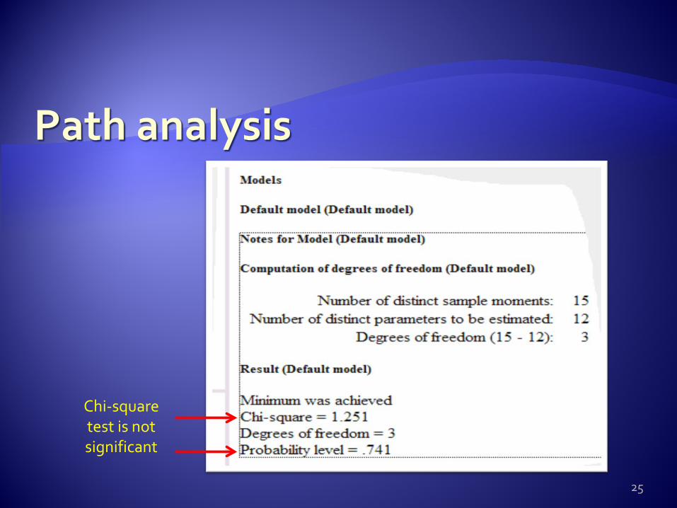
25
Chi-square test is not significant

Unstandardized graphic output
26
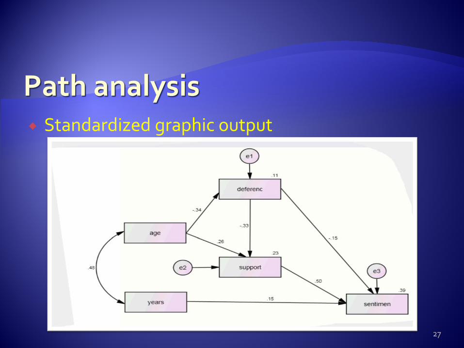
Standardized graphic output
27

Choices of model fit indexes Reporting CMIN, RMSEA, and one of the baseline fit
measures. If there is model comparison, also report one of the
parsimony measures and one the information theory measures.
28

Model fit
29
The closer RMR is to 0, the better the model fit. Rule of thumb: RMR should be < .10, or .08, or .06, or .05 or even .04.

Model fit
30
Rule of thumb: a value of the RMSEA of about 0.05 or less would indicate a close fit of the model in relation to the degrees of freedom.

Model fit
31
NFI values above .95 are good. RFI, IFI, TLI, and CFI values close to 1 indicate a very good fit.

Model fit Chi-square: χ2 = 1.25, df = 3, p = .74 Root-mean-square error of approximation (RMSEA): it
is equal to 0.00 (<.05 is acceptable) Goodness-of-fit index (GFI): .997 (>.95 is acceptable)
32

Model fit
33

Path diagram
34

This example: 4 tests: knowledge, value, satisfaction, and performance. Each test was randomly split into two halves, and each half was scored separately.
Measurement model The portion of the model that specifies how the
observed variables depend on the unobserved, or latent, variables is sometimes called the measurement model.
The current model has four distinct measurement submodels.
35

The scores of the two split-half subtests, 1knowledge and 2knowledge, are hypothesized to depend on the single underlying latent variable, knowledge.
According to the model, scores on the two subtests may still disagree, owing to the influence of measurement errors.
36

Measurement model (e.g.) 1knowledge and 2knowledge are called indicators of the
latent variable knowledge.
37
Measurement model
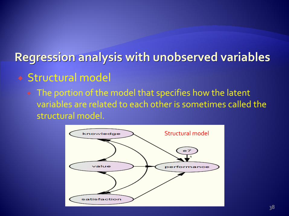
Structural model The portion of the model that specifies how the latent
variables are related to each other is sometimes called the structural model.
38
Structural model

Model identification It is necessary to fix the unit of measurement of each
unobserved variable by suitable constraints on the parameters.
Find a single-headed arrow leading away from each unobserved variable in the path diagram, and fix the corresponding regression weight to an arbitrary value such as 1.
If there is more than one single-headed arrow leading away from an unobserved variable, any one of them will do.
39

Text output
40
The hypothesis that current Model is correct is accepted.

41
Standardized regression weights

Reliability estimates
42
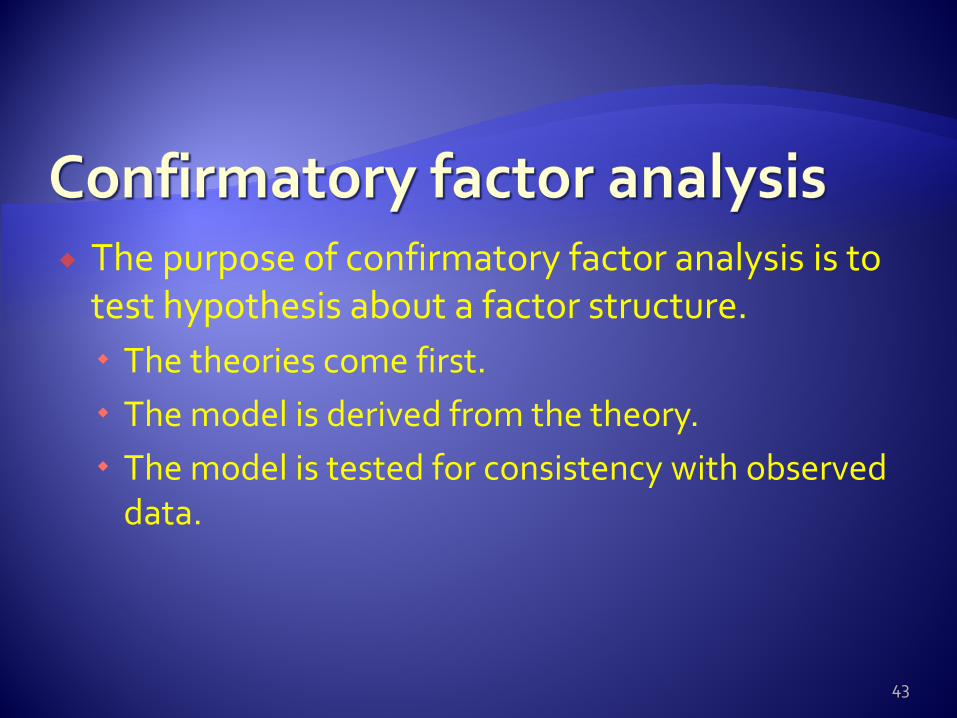
The purpose of confirmatory factor analysis is to test hypothesis about a factor structure. The theories come first. The model is derived from the theory. The model is tested for consistency with observed
data.
43

Diagram of CFA model
44
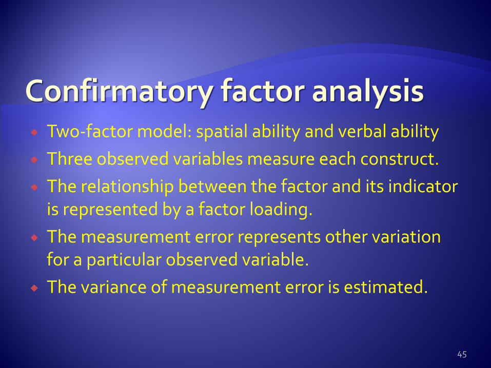
Two-factor model: spatial ability and verbal ability Three observed variables measure each construct. The relationship between the factor and its indicator
is represented by a factor loading. The measurement error represents other variation
for a particular observed variable. The variance of measurement error is estimated.
45

Model summary
46

Regression weights
47

Path diagram with standardized estimates displayed.
48

Squared multiple correlations
49

The squared multiple correlations can be interpreted as follows: To take wordmean as an example: 71% of its variance is accounted for by verbal ability. The remaining 29% of its variance is accounted for by the
unique factor e6. If e6 represented measurement error only, we could say
that the estimated reliability of wordmean is 0.71. 0.71 is an estimate of a lower-bound on the reliability of
wordmean.
50

Model fit Chi-square: χ2 = 7.85, df = 8, p = .45 Root-mean-square error of approximation (RMSEA): it
is equal to 0.00 (<.05 is acceptable) Goodness-of-fit index (GFI): .966 (>.95 is acceptable)
51

AMOS allows us to compare multiple samples across the same measurement instrument or multiple population groups (e.g., males vs. females).
We are going to use the data from IBM SPSS company (the previous data for CFA).
We want to test the equality of the factor loadings for two separate groups of school children, girls and boys.
52

Before testing measurement invariance across groups, we need test individual mode first.
If consistency is found, then we will proceed to do multiple groups testing.
The goal of testing for measurement invariance is to determine if the same SEM model is applicable across groups.
53

The general procedure is to test measurement invariance between the unconstrained model for all groups combined, then for a model with constrained parameters (parameters are constrained to be equal between the groups).
If the chi-square difference statistic is not significant between the original and constrained models, then we conclude that the model has measurement invariance across groups.
54

Which parameters are constrained to be equal? The selection of parameters to constrain depends on our research questions. Invariant factor loadings Invariant structural relations among latent variables
If lack of measurement invariance is found, the meaning of the latent construct is shifting across groups.
55

First draw a diagram for a single group
56
By default, Amos Graphics assumes that both groups have the same path diagram, so the path diagram does not have to be drawn a second time for the second group.

Select Manage Groups from the Analyze menu. Name the first group Girls.
Click on the New button to add a second group to the analysis. Name this group Boys.
Click the New button successively to add additional groups as needed.
57

58
Click
Type Boys

Select data sets: Use of the Grouping Variable and Group Value buttons. Select the Grouping Variable > identify the grouping
variable within a database > Click the Group Value button > select which value of the grouping variable represents the group of interest.
59

File > Data files
60

Open data files
61

We will name the variances, covariances, and regression weights in both the Girls and Boys models.
We will name the parameters in Girls’ model first. Use the Object Properties dialog box. Uncheck the box
for “All groups”, so you can give the variances different names in the two groups.
To name these parameters for the Boys model, highlight “boys” and go through the same procedure as before, use different names for variances, covariance, and factor loadings.
62

There is a good way to name parameters. Go to Plugins > Click Name Parameters.
63
Check Covariances, Regression weights, and Variances

We give parameters different names for Boys group. Here is a example:
64
Make sure All groups is NOT
checked
New name for Boys group

For Girls group
65
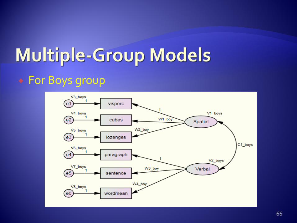
For Boys group
66

Double-click on the Default Model label shown on the left side of the path diagram window.
The Manage Models window is open.
67
You can rename the default model as something meaningful (we name it Original model).
Click New, a new model that imposes a set of equality constraints on the default model such that the unstandardized factor loadings are equal across boys' and girls' groups (we name this model Equal loading model).
Identify the four pairs relevant factor loadings of interest in the girls group and the boys group. By double-clicking on c1 and then double-clicking on c2.
68

69
Manage models
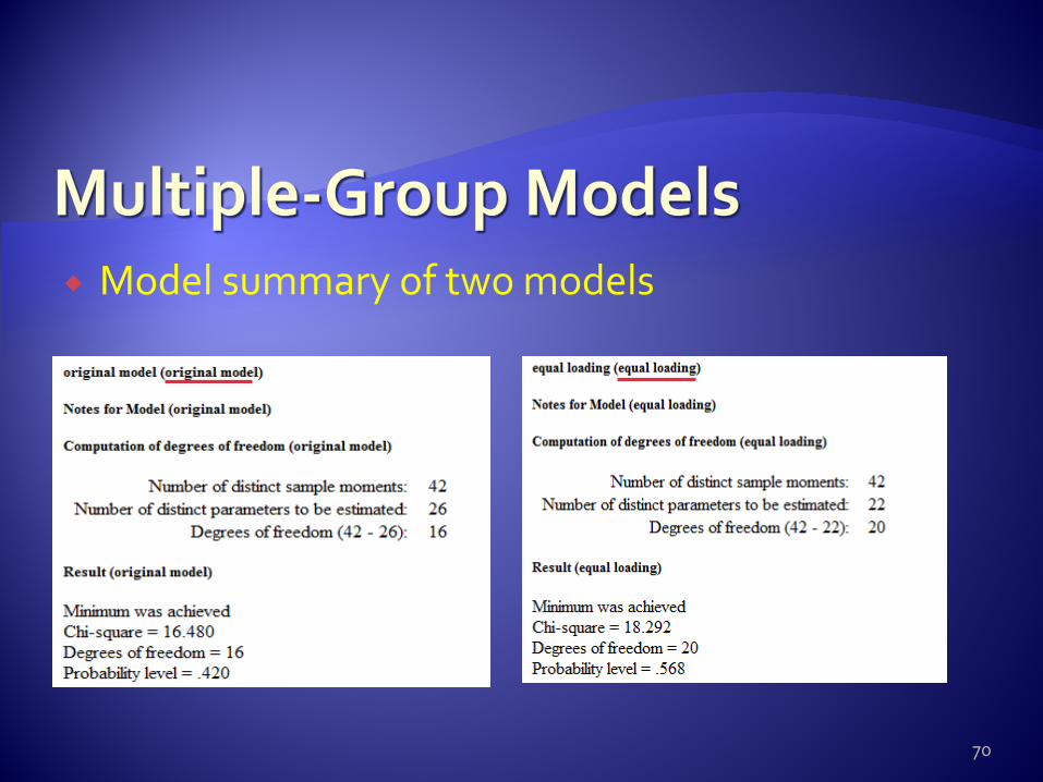
Model summary of two models
70

Model parameters for Girls
71

Model parameters for Boys
72

Model fit: we can use CFI, NCP, and GFI because they are independent of model complexity and sample size.
73

Model comparison
74

The Chi-square difference of two models is 18.292-16.480 = 1.812.
The results from this model comparison (Chi-square = 1.812 with 4 DF, p =.77 ) suggest that imposing the additional restrictions of four equal factor loadings across the gender groups did not result in a statistically significant worsening of overall model fit.
AMOS assumes that the baseline model (our original model) is true. The model (equal loading model) that specifies a group-invariant factor pattern, is supported by the sample data.
75

Another way to do multiple group analysis The first step: set up groups (give names for each
group). Go to analyze > Manage Groups The second step: open data. Go to File > Data Files.
76

Go to Analyze > Multiple-Group Analysis
77

Four different models are obtained.
78
Four models test invariances of measurement weights, structural covariances, and measurement residuals.

Model for Girls (AMOS automatically assigns names for each parameter).
79

Model for Boys
80

Model summary: original model (unconstrained)
81

Model summary: Measurement weights model
82

Model summary: Structural covariances model
83

Model summary: Measurement residuals model
84

Model fit
85
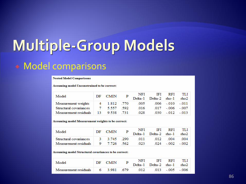
Model comparisons
86
If we find non-invariance across groups, the next step is to know what is causing this within the model. Usually, start with the factor loadings. Then, test structural weights.
87

Nested model comparisons work by imposing a constraint or set of multiple constraints on a starting or less restricted model to obtain a more restricted final model.
Example: we want to compare the equality of factor loadings with a CFA model.
88
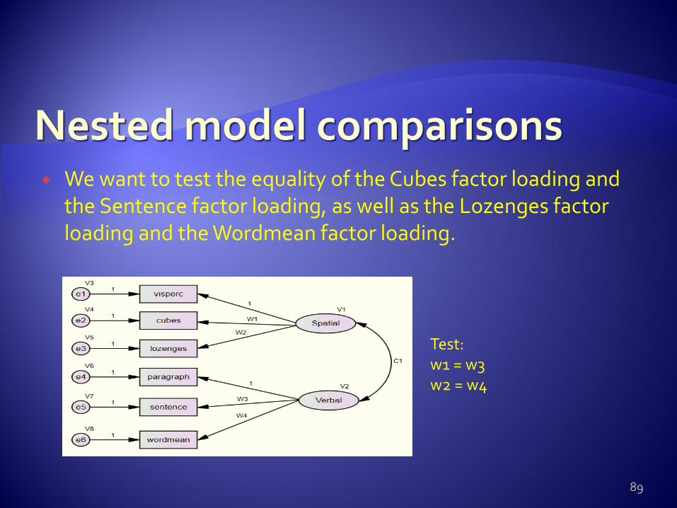
We want to test the equality of the Cubes factor loading and the Sentence factor loading, as well as the Lozenges factor loading and the Wordmean factor loading.
89
Test: w1 = w3 w2 = w4

Next, double-click on the section of the AMOS diagram window labeled Default Model.
Manage Models window is open.
90

Model comparison
91

Conclusion: The nested model comparison that assesses the worsening
of overall fit due to imposing the two restrictions on the original model shows a statistically significant chi-square value of 12.795 with 2 DF, resulting in a probability value of .002.
That the two models differ indicates that constraining the parameters in the default model to obtain the equal loadings model results in a substantial worsening of overall model fit.
Therefore, we reject the equal factor loadings model in favor of the original model.
92

The bootstrap technique It is a resampling procedure Multiple subsamples of the same size as the parent
sample are drawn randomly from the original data. Parameter estimates are computed for each
subsample.
93

When we use bootstrapping Data fail to meet the assumption of multivariate
normality. Presence of excessive kurtosis. Data are from a moderately large sample.
94

Example: path diagram
95

Assess multivariate normality: Go to View > Analysis Properties > Check Test for normality and outliers.
96

Assess multivariate normality
97
The multivariate kurtosis value of 13.167 is Mardia's coefficient. Critical ratio (c.r.)values of 1.96 or less mean there is non-significant kurtosis. Values of 7.979 > 1.96 mean there is significant non-normality.

Assess multivariate normality
98
1.Malanobis d-squared distance for a case, the more it is improbably far from the solution centroid under assumptions of normality. 2.The cases are listed in descending order of d-square. 3.We may consider the cases with the highest d-squared to be outliers and might delete them from the analysis. 4.This should be done with theoretical justification (ex., rationale why the outlier cases need to be explained by a different model). 5.After deletion, it may be the data will be found normal by Mardia's coefficient when model fit is re-run.
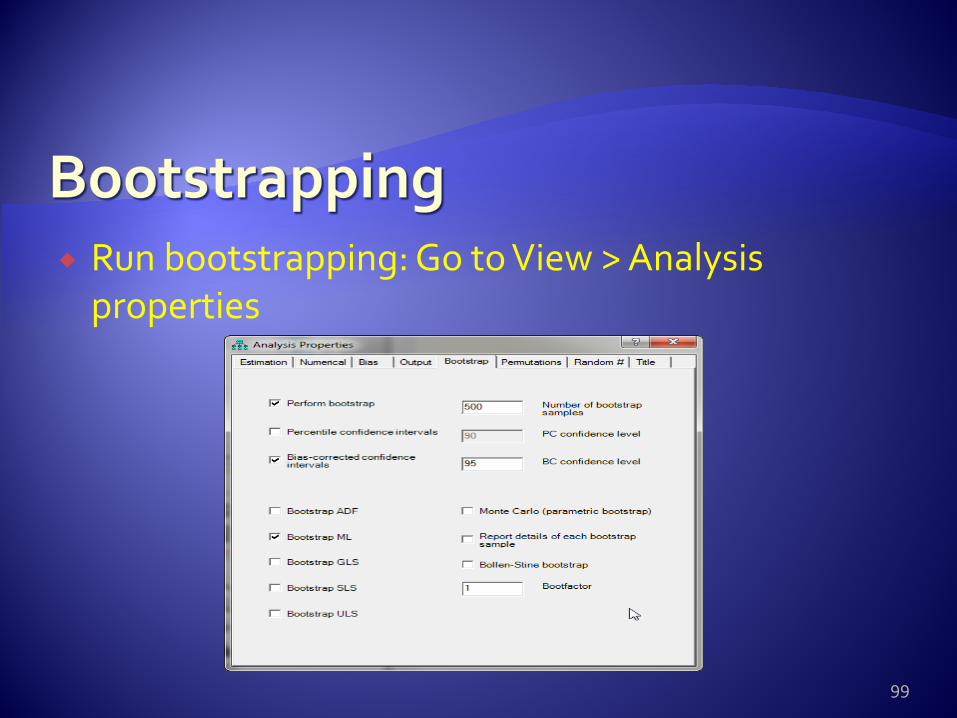
Run bootstrapping: Go to View > Analysis properties
99

100
Bootstrap ML estimates 1. The first column (SE) is Bootstrap
estimate of the standard error fro the parameter.
2. The second column (SE-SE)is standard error of bootstrap standard error itself.
3. The third column (Mean): is the mean parameter estimate computed across 500 subsamples.
4. The fourth column (Bias): represents the difference between the original mean estimate and bootstrap mean estimate.
5. The fifth column (SE-Bias): standard error of the bias estimate.
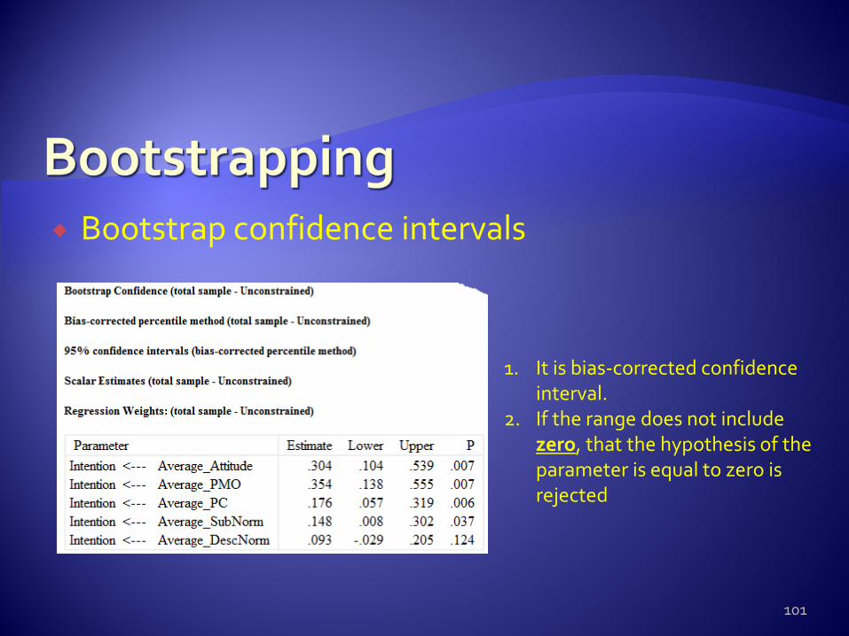
Bootstrap confidence intervals
101
1. It is bias-corrected confidence interval.
2. If the range does not include zero, that the hypothesis of the parameter is equal to zero is rejected

It is used to study change. Latent growth analysis on individual and group
levels. The measurements are taken 3 or more times
(longitudinal data). Intercept The initial value, the average or mean of the outcome we
are interested in. Think about this: for each individual in the study,
everybody has an intercept of a certain value.
102

Slope How much the curve grows over time, an average or
mean rate of growth. Each individual has a slope.
Goal of LGM Understand the average change. Understand individual variation in change.
103

Example: a longitudinal study with 4-time points data set. We want to know the change of alcohol drinking over time. a28, b28, c28, and d28 are variables we measured. The regression weights from intercept to measured
variables are fixed to 1. In this way, we establish the initial level of alcohol drinking.
The path values from slope to measured variables are also fixed at a set of continuous values (time intervals).
104

Diagram
105

Fixing the values from the slope is how we identify model growth.
Parameters Mean and variance of intercept: Mean intercept is the
average start value. The variance of intercept reflects the variation of individual start value.
106

Parameters Mean and variance of slope: Mean slope is the average of
rate of change. The variance of the slope reflects the extent to which individuals have different rates of change.
Covariance: to test whether individuals who start higher (higher intercepts) also change at a faster rate (higher slope).If such a relationship exists, we expect the covariance to be significant.
107

From AMOS, choose Plugins > Growth Curve Model.
Enter the number of measures for the number of time points.
In this example, we would enter 4 for the number of time points .
Choose View > Analysis Properties > Estimation tab. Check the Estimate Means and Intercepts check box.
108

Model identifications Right-click on the latent variable circles (labeled ICEPT
and SLOPE by AMOS) and select Object Properties. Remove the 0 constraints on the means. Fix the
variance to zero for ICEPT and SLOPE. Right-click on each of the 4 error variance circles and
select Object Properties. Fix their mean values to 0 and set their variance values to 1.00.
109

For each of the paths connecting the error circles to the observed variables, replace the original value of 1.00 with the new parameter name.
Add two new error terms to the ICEPT and SLOPE latent variables.
For the newly-created error terms, fix their mean values to 0 and their variance values to 1.00.
Next, replace the 1.00 values for the path arrows connecting errors to ICEPT and Slope. Name the newly freed parameters.
110
Remove the covariance double-headed arrow between ICEPT and SLOPE.
Place the covariance double-headed arrow between two new error terms and give a new name to the covariance.
111

Text output
112

Text output
113
1. The mean intercept value of 1.35 indicates that the average starting amount of alcohol drinking was 1.35 units. 2.The mean slope value was .11. It means the average rate of change is .11 units. 3.The correlation between the intercepts and the slopes was 2.09. 4. The means were statistically significant when tested with the null hypothesis that their true values are zero in the population from which this sample was drawn.
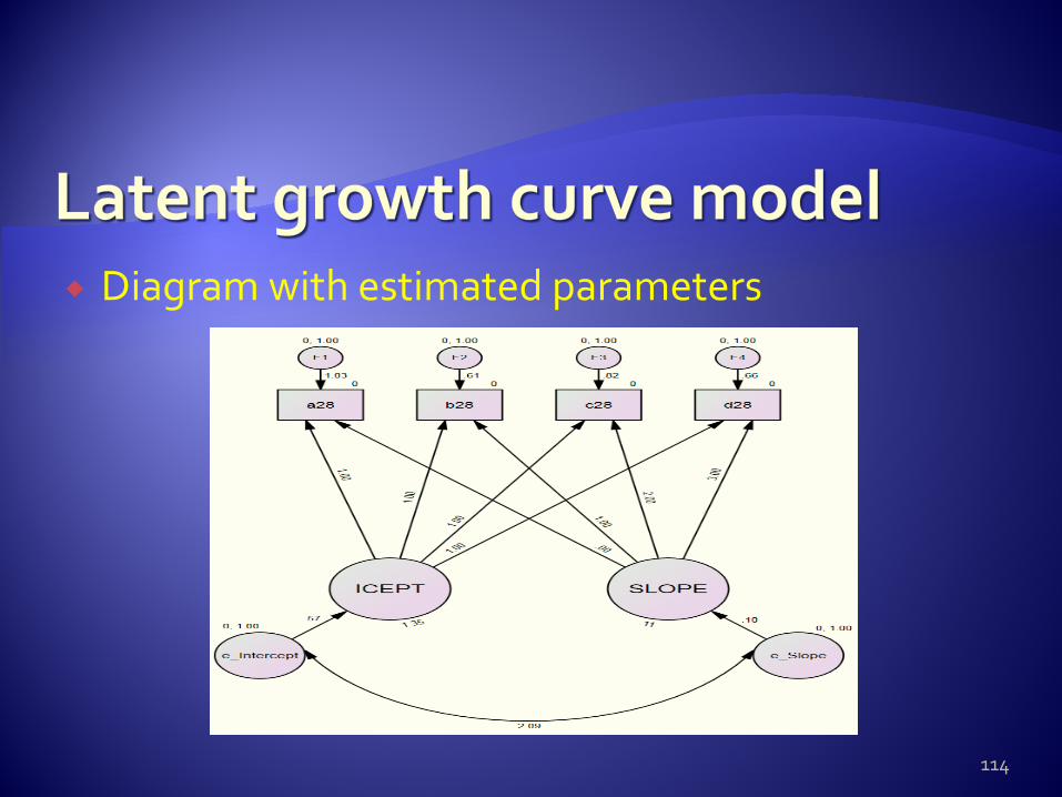
Diagram with estimated parameters
114

The intercept indicates a statistical significant mean alcohol use at the initial level (i.e., at baseline) and the slope mean indicates a significant average increase, via a liner functional form.
This alcohol use in adolescents is expected to increase by .11 each studied time period, beginning with an average score of 1.35.
115

We also want to know the extent to which adolescents in the sample vary around their group average (mean) trajectories in alcohol use.
This can be evaluated by looking at the variances. The corresponding variances ( .57 for intercept and
.30 for slope) are statistically significant, indicating significant individual variability in the initial level and rate of change (growth) in alcohol use across the four waves of measurement.
116

Hoyle, R. H. (1995). Structural equation modeling: Concepts, issues, and applications. Thousand Oaks, CA: Sage Publications, Inc.
Raykov, T. & Marcoulides, G. A. (2000). A first course in structural equation modeling. Mahwah, NJ: Lawrence Erlbaum Associates, Inc.
Schumacker, R. E. & Lomax, R. G. (2004). A beginner’s guide to structural equation modeling. Mahwah, NJ: Lawrence Erlbaum Associates, Inc.
AMOS 19.o user’s guide. IBM SPSS, Chicago.
117

118