
Selling a Cheaper Mousetrap: Wal-Mart’s Effect on Retail · PDF fileSelling a Cheaper...
36
Selling a Cheaper Mousetrap: Wal-Mart’s Effect on Retail Prices Emek Basker * University of Missouri First Draft: December 2003 This Draft: March 2005 Abstract I quantify the price effect of a low-cost entrant on retail prices using a case-study approach. I consider the effect of Wal-Mart entry on average city-level prices of various consumer goods by exploiting variation in the timing of store entry. The analysis combines two unique data sets, one containing opening dates of all US Wal-Mart stores and the other containing average quarterly retail prices of several narrowly-defined commonly-purchased goods over the period 1982-2002. I focus on 10 specific items likely to be sold at Wal-Mart stores and analyze their price dy- namics in 165 US cities before and after Wal-Mart entry. An instrumental-variables specification corrects for measurement error in Wal-Mart entry dates. I find robust price effects for several products, including shampoo, toothpaste, and laundry de- tergent; magnitudes vary by product and specification, but generally range from 1.5-3% in the short run and four times as much in the long-run. JEL Numbers: L130, L810, E310 Keywords: Wal-Mart, Competition, Prices, Market Size * Comments welcome to: [email protected]. A previous version of this paper was presented at Illinois State University, UC-Berkeley, University of Nevada - Las Vegas, Federal Trade Commission, the 2004 Missouri Economic Conference and the 2004 International Industrial Organization Conference (Chicago). I thank Saku Aura, Emin Dinlersoz, Bengte Evenson, Luke Froeb, Eric Gould, Saul Lach, Mark Lewis, Dave Mandy, Mike McCracken, Chuck Moul, Peter Mueser, Mike Noel, David Parsley, Dan Rich, John Stevens, Chad Syverson, Ken Troske, Pham Hoang Van, and seminar participants for helpful conversations and comments. I also thank Sean McNamara and David Parsley for sharing ACCRA data with me, and Aliya Kalimbetova and Loren Risker for research assistance. All remaining errors are my own.
Transcript of Selling a Cheaper Mousetrap: Wal-Mart’s Effect on Retail · PDF fileSelling a Cheaper...

Selling a Cheaper Mousetrap
Wal-Martrsquos Effect on Retail Prices
Emek Baskerlowast
University of Missouri
First Draft December 2003This Draft March 2005
AbstractI quantify the price effect of a low-cost entrant on retail prices using a case-studyapproach I consider the effect of Wal-Mart entry on average city-level prices ofvarious consumer goods by exploiting variation in the timing of store entry Theanalysis combines two unique data sets one containing opening dates of all USWal-Mart stores and the other containing average quarterly retail prices of severalnarrowly-defined commonly-purchased goods over the period 1982-2002 I focus on10 specific items likely to be sold at Wal-Mart stores and analyze their price dy-namics in 165 US cities before and after Wal-Mart entry An instrumental-variablesspecification corrects for measurement error in Wal-Mart entry dates I find robustprice effects for several products including shampoo toothpaste and laundry de-tergent magnitudes vary by product and specification but generally range from15-3 in the short run and four times as much in the long-run
JEL Numbers L130 L810 E310
Keywords Wal-Mart Competition Prices Market Size
lowastComments welcome to emekmissouriedu A previous version of this paper was presented at IllinoisState University UC-Berkeley University of Nevada - Las Vegas Federal Trade Commission the 2004 MissouriEconomic Conference and the 2004 International Industrial Organization Conference (Chicago) I thank SakuAura Emin Dinlersoz Bengte Evenson Luke Froeb Eric Gould Saul Lach Mark Lewis Dave Mandy MikeMcCracken Chuck Moul Peter Mueser Mike Noel David Parsley Dan Rich John Stevens Chad SyversonKen Troske Pham Hoang Van and seminar participants for helpful conversations and comments I also thankSean McNamara and David Parsley for sharing ACCRA data with me and Aliya Kalimbetova and Loren Riskerfor research assistance All remaining errors are my own
ldquoWal-Martrsquos mania for selling goods at rock-bottom prices has trained consumers toexpect deep discounts everywhere they shop forcing competing retailers to followsuit or fall behindrdquondash Washington Post November 6 2003
ldquoEven if you donrsquot shop at Wal-Mart the retail powerhouse increasingly is dic-tating your product choices ndash and what you pay ndash as its relentless price cuttinghelps keep inflation lowrdquondash USA Today January 29 2003
1 Introduction
In most models of imperfect competition entry of a lower-cost competitor reduces output
prices The effect is larger the smaller the initial number of firms and the higher are cross-price
elasticities of demand In this paper I quantify the price effect of a low-cost entrant on retail
markets using a case study of Wal-Mart entry and show that Wal-Martrsquos price impact can be
quite large The analysis combines data on the opening dates of all US Wal-Mart stores with
average city-level retail prices of several narrowly-defined commonly-purchased goods over the
period 1982-2002 I focus on 10 specific items likely to be sold at Wal-Mart stores and analyze
their price dynamics in 165 US cities before and after Wal-Mart entry I find price declines of
15-3 for many products in the short run with the largest price effects occurring for aspirin
laundry detergent toothpaste and shampoo Long-run price declines tend to be much larger
and in some specifications range from 7-13 These effects are driven mostly by relatively small
cities which have high ratios of retail establishments to population
Wal-Martrsquos low labor costs and the retail chainrsquos logistics and distribution innovations make
it the prototypical low-cost entrant Broadly there are two mechanisms by which Wal-Martrsquos
expansion could have affected retail prices and consumer inflation rates an aggregate mecha-
nism and a market-specific mechanism The aggregate mechanism works through Wal-Martrsquos
interactions with both suppliers (manufacturers and importers) and other large retail chains
This mechanism can lower prices in communities not served by Wal-Mart if it leads to lower
costs for other retailers1 The market-specific mechanism works through competition (and
1The argument for this mechanism is as follows By demanding lower prices from suppliers Wal-Mart forcesmanufacturers to cut costs possibly by relocating overseas Competing retail chains (notably Target but alsomany smaller chains) also increase efficiency by emulating Wal-Martrsquos innovations in logistics and distribution(McKinsey Global Institute [22]) The result is lower prices in chain stores across the country some in locationsthat have no Wal-Mart stores
1
possibly learning) at the local level
The focus of this paper is on the second mechanism Wal-Martrsquos entry into a given market
(city or town) can lower prices by increasing the competitive pressure incumbents (and future
entrants) face This is the prediction of most standard imperfect-competition models such as
differentiated-product Bertrand competition and a spatial-competition model and also of many
models with equilibrium price dispersion (such as Reinganum [25])2
Although these theories make consistent predictions about the price impact of entry very
little empirical work has been done to quantify these effects I test these predictions on average
prices of 10 specific goods such as toothpaste Coke and jeans by exploiting exogenous variation
in the timing of store entry in different markets I combine two unique data sources on Wal-
Mart store locations and retail prices in 165 US cities over a 20-year period 1982-2002 The
Wal-Mart data include store locations and opening dates of all US Wal-Mart stores Price data
from the American Chamber of Commerce Research Association (ACCRA) consist of average
retail prices of 10 products across multiple establishments in each city
The methodology follows Basker [3] which examines the employment effects of Wal-Mart
entry with two innovations In Basker [3] I consider the effect of Wal-Mart entry on county-
level employment in the retail and wholesale sectors using 1749 counties (slightly more than
half of all US counties) Because price data are available at the city (or town) level rather than
the county level I disaggregate the Wal-Mart data to the city level for this study In addition
because price data are collected quarterly I perform the analysis using quarterly rather than
annual data
I define the ldquoeffectrdquo of Wal-Mart entry broadly For example if Wal-Mart entry induces the
exit of an incumbent drugstore the long-run price effect I isolate combines the effect of both
the entry and the exit By estimating separate short- and long-run price effects I attempt to
separate these issues If Wal-Mart entry spurs other entries or leads to increased differentiation
among incumbents this too is incorporated in the net effect
I find that the price effect of Wal-Mart entry differs by product and city size For several
products including toothpaste shampoo aspirin and laundry detergent Wal-Mart entry re-
duces average retail prices by an economically large and statistically significant 7-13 in the
long run These results have real implications if the market basket of low-income shoppers
2The products whose prices I consider are homogeneous but the shopping experience including location andservice may be better described as differentiated
2
declined by this full amount the income effects could be very large Results are driven by
Wal-Martrsquos effects in smaller cities with more retail establishments per capita where retail
establishments tend to be smaller and the retail environment is less competitive
The remainder of this paper is organized as follows Section 2 provides background infor-
mation on Wal-Mart Section 3 describes the data The empirical methodology is outlined in
Section 4 and results are presented in Section 5 Section 6 concludes with a discussion of the
magnitude of the price effect and its implications
2 Wal-Mart Background
The first Wal-Mart store opened in Rogers Arkansas in 1962 By the time the company be-
came publicly traded in 1969 it had 18 stores throughout Arkansas Missouri and Oklahoma
Wal-Mart slowly expanded its geographical reach building new stores and accompanying dis-
tribution centers further and further away from its original location and continued at the same
time to build new stores in areas already serviced Figure 1 shows maps of the 48 contiguous
states with locations of Wal-Mart stores over time (in 1982 1993 and 2002) to illustrate this
point In the beginning of the period Wal-Martrsquos sales accounted for approximately 02 of
all US retail sales by the end of it Wal-Mart had approximately 2900 stores in all 50 states
and about 800000 employees in the United States and accounted for approximately 5 of all
US retail sales
Wal-Mart is extremely efficient even compared with other ldquobig-boxrdquo retailers Lehman
Brothers analysts have noted Wal-Martrsquos ldquoleading logistics and information competenciesrdquo
(Feiner [12]) The Financial Times has called Wal-Mart ldquoan operation whose efficiency is
the envy of the worldrsquos storekeepersrdquo (Edgecliffe-Johnson [11]) Wal-Martrsquos competitive edge is
driven by a combination of conventional cost-cutting and sensitivity to demand conditions and
by superior logistics and distribution systems The chainrsquos most-cited advantages over small
retailers are economies of scale and access to capital markets whereas against other large retail
chains the most commonly cited factor is superior logistics distribution and inventory con-
trol3 Employing exclusively non-union workers may be another source of cost-savings relative
to other retailers4
3Details on Wal-Martrsquos operations can be found in Harvard Business Schoolrsquos three case studies about Wal-Mart (Ghemawat [15] Foley and Mahmood [13] and Ghemawat and Friedman [16])
4On the other hand Wal-Mart is said to match the union wage in markets where it competes directly with
3
Figure 1 Locations of Wal-Mart Stores 1982 1993 2002
4
3 Data
To assess Wal-Martrsquos effect on retail prices I combine data on the locations and opening dates
of Wal-Mart stores with retail price data
31 Retail Prices
Retail prices are obtained from the American Chamber of Commerce Research Association I
use quarterly prices of 10 products in 165 cities over 21 years from 1982-2002
The American Chamber of Commerce Research Association (ACCRA) through local Cam-
bers of Commerce surveys 5-10 retail establishments in the first week of each quarter in par-
ticipating cities Participating cities vary from quarter to quarter with some cities moving in
and out of the sample frequently while others are included more regularly 250-300 cities are
surveyed each quarter during the sample period Of these I selected the 165 cities for which
data from at least 50 quarters were available (including both current price and lagged price)
Each quarter between 100-140 cities are in the sample
The prices collected by ACCRA cover approximately 50 goods and services From the list
of items I selected 10 goods that were homogeneous or nearly so and likely to be sold at most
Wal-Mart stores (I exclude groceries and alcoholic beverages because most Wal-Mart stores
over the sample period do not include a grocery section) The selected products are listed in
Table 1 I begin my sample period in 1982 because most of these products were introduced into
the ACCRA price list in that year5
While these data are the best available local price data that span such a long time-series as
well as cross-section of cities covering specific prices they have some drawbacks One problem
is that the individual stores from which prices are collected cannot be identified if they include
Wal-Mart stores we will not be able to distinguish the direct impact of Wal-Mart (eg due to
charging lower prices than other stores) from the indirect impact through competitive pressure
on other stores Somewhat mitigating this concern the ACCRA manual urges its price collectors
nationwide to ldquo[s]elect only grocery stores and apparel stores where professional and managerial
households normally shop Even if discount stores are a majority of your overall market they
unionized retailers (Saporito [26])5For some products there is a change in the brand orand size of the product during the time period but since
quarter dummies will be controlled in the analyses below changes in the price due to such shifts are accountedfor We assume that the price response to Wal-Mart entry is the same across these alternatives
5
shouldnrsquot be in your sample at all unless upper-income professionals and executives really shop
thererdquo (ACCRA [1] p 13) If price surveyors follow this instruction we may estimate a lower
bound of Wal-Martrsquos impact because Wal-Mart and its most direct competitors are unlikely to
be included
Another potential problem is measurement error in prices Measurement error may come
from several sources The most likely are errors made by price surveyors in the tallying of
individual prices (eg copying prices incorrectly from store shelves) the average price reported
by ACCRA will be sensitive to such errors This type of error is likely to be idiosyncratic
uncorrelated over time or across products Differences across cities or surveyors in the types
of establishments surveyed or the size of the geographic area covered may also be treated as
errors these are less innocuous because they are likely to be correlated over time within a city I
discuss this issue and the problems it creates along with possible remedies in the methodology
section
32 Wal-Mart Stores
The Wal-Mart store data are described in detail in Appendix 1 of Basker [3] I briefly review
the data sources
I collected data on the locations and opening dates of 2382 Wal-Mart stores in the United
States from Wal-Mart annual reports Wal-Mart editions of Rand McNally Road Atlases and
annual editions of the Directory of Discount Department Stores6 The available data include
store location (by city) and store number Opening years of individual stores can be inferred
by comparing lists of existing stores from consecutive years7 Table 2 (reproduced from Basker
[3]) summarizes these sources8
From these lists I create the indicator variable WMopenjt which takes on the value of 1
if the directories and store lists suggest that a Wal-Mart store exists in city j in quarter t and
zero otherwise While this assignment is simple in the calendar years preceding or following
the year of entry the exact quarter of entry is not known from these lists so quarterly values
6Requests for store-opening data from Wal-Mart corporation were denied I have also tried to obtain openingdates from local newspapers but only succeeded in a handful of cases
7Vance and Scott [30] list store entries to 1969 the year the company became publicly traded8For the years 1990-1993 in which no satisfactory store list allowing identification of Wal-Mart stores in a city
exists (the Directory of Discount Department Stores was not updated during those years) I assign opening datesto stores according to a probabilistic algorithm that uses information on the number of stores opening in eachstate each year State-level data are obtained from Wal-Mart annual reports [31] This procedure is detailed inBasker [3] Appendix 1
6
of WMopenjt have to be imputed for the year of entry I obtain the empirical distribution
of entry dates over the year from Wal-Martrsquos web site which provides exact opening dates for
all store openings over the three-year period July 2001 - June 2004 (Quarterly probabilities
are approximately 29 26 26 and 19) So for a store that opened in 1986 I assign the
variable WMopen a value of 0 up to and including the first quarter of 1986 (since the first-
quarter observation gives prices in the first week of January) 029 in the second quarter 055
in the third quarter 081 in the fourth quarter and 1 from the first quarter of 1987 onwards9
I also construct a set of identifiers of Wal-Mart planned entry dates using a combination
of company-assigned store numbers (available from the Rand McNally atlases) and the net
change in the number of stores each year (from company annual reports) Wal-Mart assigns
store numbers roughly in sequential order with store 1 opening first followed by store 2
and so on store numbers appear to be assigned early in the store planning process Following
this practice I assign planned entry dates to stores sequentially based on their store numbers
holding fixed (at actual levels) the total number of new stores to open each year For example
since there were 18 stores at the end of 1969 and 20 new stores opened in 1970 I assign 20
stores (numbers 19-38) the planned entry year 1970 This assignment assumes that the number
of planned entries in 1970 was the same as the actual number of entries that year
Within a calendar year I assign the first 29 of stores to the first quarter (so they are
assumed to be open by the second quarter) the next 26 to the second quarter another 26
to the third quarter and the remainder to the fourth quarter (so they are open by the first
quarter of the following year)
This assignment method provides a good approximation to the likely order in which the
stores were planned Aggregating these store-level entry dates to the city-quarter level I con-
struct the indicator variable WMplanjt which equals 1 if city j would have had a Wal-Mart
store in quarter t had the stores opened in the order in which they were planned In the most
specifications below I use only the opening dates (both WMopen and WMplan) for the first
Wal-Mart store to open in each city but I also estimate two models that try to get at the effect
of subsequent Wal-Mart entries10
9The resulting variable WMopenjt is equal to either 0 or 1 in 96 of the observations Most of the ob-servations in which WMopenjt takes on values strictly between 0 and 1 representing the probability that aWal-Mart store exists occur during the years (1990-1993) when store directories were not updated (see footnote8) Replacing this imputation with an indicator variable which equals 1 if the probability of a Wal-Mart storeexceeds 50 and zero otherwise does not meaningfully change any of the results in the paper
10An alternative to imputing quarterly data for Wal-Mart is to aggregate the price data to annual frequency
7
Table 1 ProductsProduct Description Pricelowast
Dru
gsto
reP
rodu
cts
Aspirin 100-tablet bottle Bayer brand (to 19943) $ 49605oz Polysporin ointment (from 19944) $ 456
Cigarettes Carton Winston king-size (85mm) $1969Coke 2-liter Coca Cola excluding deposit $ 156Detergent 49oz TideBoldCheer laundry detergent (to 19913) $ 339
42oz TideBoldCheer laundry detergent (19914-19963) $ 39760oz Cascade dish washing powder (from 19964) $ 302
Kleenex 200-count Kleenex tissues (to 19834) $ 146175-count Kleenex tissues (from 19841) $ 134
Shampoo 11oz bottle Johnsons Baby Shampoo (to 19912) $ 42115oz Alberto VO5 (from 19913) $ 129
Toothpaste 6-7oz Crest or Colgate $ 240
Clo
thin
g
Shirt Mans dress shirt Arrow $3019Pants Levis 501505 jeans rinsedwashedbleached size 28-36 (to 19994) $3328
Mens Dockers ldquono wrinklerdquo khakis size 28-36 (from 20001) $3572Underwear 3 boys cotton briefs Fruit of the Loom (to 19834) $ 729
3 boys cotton briefs size 10-14 cheapest brand (from 19841) $ 536lowast Average price over entire sample period in 2000 dollars
Table 2 Directory Sources for Wal-Mart Opening DatesYears Source1962-1969 Vance and Scott (1994)1970-1978 Wal-Mart Annual Reports1979-1982 Directory of Discount Department Stores1983-1986 Directory of Discount Stores1987-1989 Directory of Discount Department Stores1990-1993 Imputed (see footnote 8)1994-1997 Rand McNally Road Atlas
8
33 Sample Cities
The sample cities determined by price-data availability are shown in Figure 2 and some
summary statistics are shown in Table 3 The average city in the sample had approximately
200000 residents in 2000 (the median city had approximately half as many residents) The
large apparent decrease in the number of establishments between 1987 and 1997 is due to a
change in Census industrial coding from SIC to NAICS (More information about the switch
from SIC to NAICS is available at httpwwwcensusgovepcdwwwnaicshtml11) The
right-skew implied by deviation between median and mean is comparable to the one obtained
from a census of US cities
Of the 165 sample cities 25 had at least one Wal-Mart store at the beginning of the sample
period All but three cities (Denver South Bend and Tacoma) had experienced entry by the
end of the sample period and three cities experienced exit
4 Empirical Methodology
41 Ordinary Least Squares (OLS) Regressions
I estimate the following regression by product
pkjt = αk + βkpkjtminus1 + θkWMopenjt
+sum
j
γkjcityj +sum
t
δktquartert +sum
j
τkjtrendt + εkjt (1)
where pkjt is the natural log of the price of product k in city j in quarter t quartert is a
quarter indicator (where t ranges from 1982q2 to 2002q4 ndash a total of 83 quarter indicators)
cityj is a city indicator trendt is a linear trend (with coefficient τkj which is specific to city
j) and WMopenjt is the Wal-Mart indicator it equals 1 if city j has a Wal-Mart store in
quarter t (From now on I suppress the k subscript it is always implied since the regressions
are estimated one product at a time)
The quarter fixed effects are intended to capture macroeconomics price fluctuations changes
in product definitions or cost of production that are common across all cities City fixed effects
This was done in a previous version of the paper with qualitatively similar results11Wal-Mart entry does not lead to sharp decreases in the number of retail establishments on average at the
county level 5 retail establishments close within 5 years of Wal-Mart entry (Basker [3])
9
Figure 2 Locations of Sample Cities
Table 3 Sample Cities Summary StatisticsPercentiles
Mean 25th 50th 75thPopulation (1980) 164322 40450 71626 172140Population (1990) 179344 44972 84021 187217Population (2000) 199797 52894 91565 217074Retail Establishments SIC (1982)lowast 1780 537 906 1736Retail Establishments SIC (1987)lowastlowast 2132 641 1069 2069Retail Establishments NAICS (1997)dagger 1037 373 515 1106Per-Capita Income (1979)Dagger 16640 15041 16351 17810Per-Capita Income (1989)Dagger 17911 16052 17346 19592Source Authorrsquos calculations from County and City Data Book Various Yearslowast Mean calculated using only 142 of 165 cities percentiles include all citieslowastlowast Mean calculated using only 145 of 165 cities percentiles include all citiesdagger Mean calculated using only 146 of 165 cities percentiles include all citiesDagger Real 2000 dollars
10
capture average (long-run) price differences across cities for example due to differential land
or labor costs City-specific time trends capture changes over time in relative prices for various
exogenous reasons trends in average income income inequality land and labor costs and the
level of competition12 If Wal-Mart entry is correlated with the sign and degree of these trends
ndash for example if Wal-Mart enters cities with declining prices earlier (or later) than cities with
rising prices ndash the estimated coefficient will be biased in regressions that omit this trend (City-
level time trends are jointly extremely statistically significant F statistics are almost always
above 10000) Put together these control variables capture three things average differences
in prices across cities different trends in prices across cities and macroeconomic shocks as well
as changes in product definitions that shift these trends
The coefficient on lagged price β is a relative ldquostickinessrdquo parameter indicating to what
extent relative prices in city j in quarter t ndash adjusting for differences in their long-run trends
ndash are unchanged from one quarter to the next If β = 0 then the price (of shampoo or
cigarettes or laundry detergent) in city j in quarter t is an iid draw with expected value
that depends only on city jrsquos price trend and any aggregate factors captured by the calendar
quarter (and possibly the presence of Wal-Mart) If β gt 0 however deviations of price from
this deterministic path last more than just one quarter so that last periodrsquos price of a product
has predictive power for this periodrsquos price The interpretation of the coefficients on the city
fixed effects and the city-specific trends depends critically on having β lt 1 ie on the price
series being stationary My estimates of β vary by product and specification but mostly lie in
the interval [07 08]13 Thus β captures the fact that price deviations from a cityrsquos ldquotrending
averagerdquo (relative to all other cities in the sample) last more than one period but decay over
time
The coefficient θ captures the instantaneous effect of Wal-Mart entry on prices Assuming
for expositional purposes that θ lt 0 and β lt 1 if prices fall by θ in the quarter of entry
there will be an additional effect of βθ the following quarter as lagged prices are now θ lower
than they were before and an additional β2θ the following quarter The long-run (asymptotic)
effect of Wal-Mart entry on prices is θ1minusβ 14 I estimate both the instantaneous and asymptotic
12The inclusion of both city fixed effects and city-specific trends allows the average price in each city to takea separate (linear) path This is a reduced-form way of controlling for variables that change at low frequencies(like income and population) without including them directly
13Parsley and Wei [23] use ACCRA price data for 48 cities over the period 1975-1994 and find strong evidenceagainst unit roots in prices and in favor of price convergence
14As with the city-level coefficients this expression depends critically on β lt 1 As note above this condition
11
effects and separately test for their significance (I use a Wald test for the non-linear test)
Figure 3 illustrates the interpretation of the coefficients Wal-Mart entry occurs at time
t0 The first panel shows the case with no price trends the second and third panels show that
the interpretation of the coefficients does not change when city-specific linear time trends are
included in the model
Because the short- and long-run effects estimated by these models are mechanically related
(through the coefficient β) I also test to see whether there is an additional long-run effect of
Wal-Mart This could occur for several reasons as some incumbents exit following Wal-Martrsquos
entry the remaining storesrsquo prices may increase over time alternatively they may decrease if
consumers are relatively unresponsive to price differences across locations in the short-run but
become more responsive over time I allow a two-step adjustment process to Wal-Mart entry
an instantaneous effect θ and a second effect φ five years (20 quarters) later15
pjt = α + βpjtminus1 + θWMopenjt + φWMopenjtminus20
+sum
j
γjcityj +sum
t
δtquartert +sum
j
τjtrendtj + εjt (2)
Figure 4 shows this specification graphically with θ and φ ldquoprice shocksrdquo T periods apart
(For simplicity trends are omitted from the figures) The long-run effect is given by θ+φmiddotβT+1
1minusβ
Depending on the relative magnitudes of θ and φ and on the sharpness of ldquodiscountingrdquo implied
by β the long-run effect may be larger or smaller than the short-run effect of Wal-Mart and
may even be of the opposite sign (as in the second panel) This is in contrast with estimates
from Equation (1) in which as long as β lt 1 long-run estimates are always of the same sign
as short-run effects and always larger in absolute terms
42 Measurement Error in Prices
ACCRA price data are subject to measurement error as discussed in Section 31 If price were
only on the left-hand side of the regression measurement error would increase the variance of
the error term without affecting any coefficient estimates But both specifications (1) and (2)
include lagged price on the right-hand side of the regression to account for the fact that prices
holds for all specifications15The choice of a five-year window is arbitrary but Basker [3] shows that within five years the retail sector
has completed its adjustment
12
θ
φ
(Θ+φβT+1) (1-β)
T
t
t0 t1
T
θ
φ
(Θ+φβT+1) (1-β)
t
t0 t1
θ
(Θ+φβT+1) (1-β)φ
T
t
t0 t1
θ θ(1-β)
t0
t
θθ(1-β)
tt0
t
θ(1-β) θ
t0
t
Figure 3 Interpreting Regression Coefficients
13
θ
φ
(Θ+φβT+1) (1-β)
T
t
t0 t1
T
θ
φ
(Θ+φβT+1) (1-β)
t
t0 t1
θ
(Θ+φβT+1) (1-β)φ
T
t
t0 t1
θ θ(1-β)
t0
t
θθ(1-β)
tt0
t
θ(1-β) θ
t0
t
Figure 4 Interpreting Regression Coefficients with Two Wal-Mart Coefficients
14
move slowly and do not return to their expected (trend-adjusted) level for several quarters
following any ldquoshockrdquo
In the presence of measurement error in prices the estimate of β is attenuated (biased
towards zero) and other point estimates including the estimate of θ are also biased If the
measurement error is solely or primarily due to errors in the process of collecting prices ndash eg
writing down a price of 079 when the true price is 097 ndash so that the errors are uncorrelated over
time we can address this problem by using pkjtminus2 the second lag of price to instrument for
pkjtminus1 Unless otherwise noted all the estimates shown below use this IV strategy to eliminate
(or at least reduce) the problem of measurement error
If measurement error is due to other causes ndash such as non-representative selection of retail
establishments in the price survey ndash twice-lagged price may not be a valid instrument For this
reason I experiment with a functional form that omits lagged price16
pjt = α + θWMopenjt +sum
j
γjcityj +sum
t
δtquartert +sum
j
τjtrendt + εjt (3)
Including lagged prices on the right-hand side of the regression is problematic for another
reason lagged price may be endogenous Endogeneity of lagged price could arise because the
error term εjt is not iid ndash for example if it follows an AR or MA process ndash in which case the
error term and lagged price will be correlated Like measurement error endogeneity of lagged
price would also yield biased estimates of Wal-Martrsquos effect in these regressions17
Instrumenting for lagged price with twice-lagged price as described above is a valid cor-
rection for endogeneity under some ndash but not all ndash conditions Specifically if the error term is
MA(1) an IV specification would be valid but if the error term is AR(1) it would not in that
case twice-lagged price (as well as any longer lag) would still be correlated with the error term
The alternative specification with no lagged price may be preferable under these conditions
(A completely exogenous instrument would be the best solution to this problem but none is
available as noted in footnote 16) While neither specification is perfect taken together the
16There is no available alternative instrument for lagged price A valid instrument needs to be correlated withlast quarterrsquos average price of a given good in a city after controlling for all the covariates but be uncorrelatedwith the error in measurement of lagged price
17The same problem would result if there is an omitted determinant of price which is correlated with laggedprice and is not captured by any of the other regressors in the model (A possible example could be entry ofanother large retailer if it depresses prices) Since the regression includes both city and time (quarter) fixedeffects to induce bias this omitted variable must vary across both time and cities and not follow a linear trendat the city level
15
two specifications tell a more complete story than either one tells alone
43 Measurement Error in Wal-Mart Data
I use instrumental-variables estimates to correct for two problems in the Wal-Mart variable
measurement error and endogeneity Inaccuracies in the directories and store lists combined
with the probabilistic method of assigning opening dates across quarters (and across years
over the period 1990-1993) lead to measurement error in the variable WMopenjt causing
attenuation bias in estimates of θ Endogeneity may also a problem even after controlling for
city-level trends if Wal-Mart entry is more likely in times of high (or low) prices relative to
the cityrsquos long-run trend In that case mean reversion alone will cause prices to fall (rise) and
the estimated coefficient θ may be spuriously negative (positive)
Measurement error in the Wal-Mart entry variable WMopenjt takes a particular form
while the entered cities are correctly identified the timing of entry may be incorrectly measured
due to errors in the directories The variable WMplanjt is also measured with error by
construction it represents the number of stores that would be open had stores always opened
in the order in which they were planned with the total number of stores opening each year is
held at its actual level and the distribution of opening dates across quarters assumed constant
ndash at 2001-04 levels ndash over the 20 year period
As long as the measurement errors in the two variables is classical and uncorrelated we can
use WMplanjt to instrument for WMopenjt The second assumption appears to be correct
it would be violated if for example stores in rural areas are completed faster than stores in
urban areas and also appear later in directories but this does not appear to be the case18
But measurement error is not classical the actual number of Wal-Mart stores in city j in
quarter t differs from the measured number by a number whose expected value is correlated
with the measured number (For example when the directories report zero Wal-Marts in town
the expected number of stores is some (small) positive number When the reported number of
Wal-Marts is one the actual number is usually either zero or one so the expected number is
less than one) This induces a slight bias in the instrumental-variables results reported here19
18There is no correlation between observable location characteristics and the time lag between the ldquoplanningdaterdquo and the opening date of a store
19Kane Rouse and Staiger [20] suggest a GMM estimator to address this problem Unfortunately due to thesize of the panel their solution is not computationally feasible in this setting While the bias could be large intheory in the static returns-to-schooling example of Kane Rouse and Staiger the bias is approximately 5 ofthe IV coefficient estimate The sign of this bias is indeterminate
16
The first-stage regression associated with Equation (1) is
WMopenjt = α + βpjtminus1 +sum
t
δtquartert + θWMplanjt +sum
j
τjtrendtj + εjt
Although the first-stage regression has a binary dependent variable I estimate the first-stage
by Ordinary Least Squares rather than a nonlinear model such as probit or logit Angrist and
Kreuger [2] caution against using a nonlinear first-stage model because unless it is exactly
right it will generate inconsistent second-stage coefficients A first-stage OLS specification in
contrast yields consistent second-stage estimates even if it is not exactly correct
This IV strategy can also correct for possible endogeneity of Wal-Martrsquos entry decision
Concerns about endogeneity have two dimensions Wal-Mart may select the cities it enters
non-randomly and it may choose the timing of entry non-randomly
The cross-sectional dimension (choice of cities) is very plausible for example Wal-Mart
may prefer to enter cities with less-competitive retail markets (hence higher pre-entry prices)
or with a larger fraction of search-savvy lower-middle income families (whose presence leads to
lower average retail prices see Frankel and Gould [14]) This concern is greatly mitigated by
the fact that Wal-Mart entry is observed in 162 of the 165 sample cities and the sample cities
are diverse with respect to all standard economic and demographic variables (see Table 3)
The timing dimension is important if Wal-Mart can schedule its entry to coincide with high
retail prices Under reasonable assumptions using WMplanjt to instrument for WMopenjt
can correct not only for measurement error but also for endogeneity in the timing of entry Of
course if there are omitted variables ndash if Wal-Martrsquos entry is correlated with other shocks to the
local retail market such as the entry or exit of other stores ndash in which case OLS estimates may
confound Wal-Martrsquos effect with price changes that happen for other reasons (Any omitted
city-specific variable that is either unchanged over this period or moves linearly will be captured
by the city fixed effects andor the city-specific trends in the model)
The identification strategy assumes that Wal-Mart plans its store entries well in advance
of entry and cannot accurately forecast exact market conditions (prices) at the time for which
entry is planned This assumption seems reasonable it can take a year and often longer to
get a property zoned acquire all the necessary building permits build and open a store for
business While Wal-Mart may want to enter any market at a time when prices are relatively
high ndash when potential profits as well as apparent benefit to consumers are highest ndash it cannot
17
predict the timing of high prices with any accuracy if the delay between planning and entry is
long enough The company may fine-tune opening dates based on current market conditions
but if the planning occurs sufficiently in advance ndash and prices are sufficiently flexible ndash then
planning dates can be treated as exogenous to retail prices at the time of Wal-Mart entry So
while the actual date of entry may be manipulated ndash moved forwards or delayed ndash to correspond
with ldquofavorablerdquo (high) price conditions the planned date of entry will be largely free of those
biases at least once we account for long-run differences in average prices across cities20
5 Results
51 OLS Results
Before proceeding to the IV results I show some results from OLS regressions of Equation (1)
Unless otherwise noted the specifications below use twice-lagged price as an instrument for
lagged price I use the term ldquoOLSrdquo to mean that the Wal-Mart variable WMopenjt is not
instrumented
Table 4 shows results from 10 separate OLS regressions Each row represents a separate
regression and shows the estimated coefficients θ (the instantaneous effect of Wal-Mart entry)
and β (the mean-reversionprice stickiness parameter) as well as the estimated long-run effect
of entry θ1minusβ Significance levels for the latter are given by the p-value from a (two-sided) Wald
test for H0 θ1minusβ = 0 So for example the average price of detergent is estimated to decline by
078 in the quarter following Wal-Mart entry and reach a decline of 386 asymptotically
OLS estimates of the price effect of Wal-Mart are negative for 9 of the 10 products (cigarettes
are the exception) and significant for three products ndash detergent shampoo and toothpaste
(although the latter is significant only at the 10 level) For these three products the estimated
short-run effect has a magnitude of 07-08 and the long-run magnitude of 35-4
The distinction between short- and long-run effects of Wal-Mart depend on the inclusion of
20A possible exception to this argument is if Wal-Martrsquos entry is correlated with the entry (or exit) of otherfirms If both the planning and the implementation of Wal-Mart entry coincides with that of other retailers ndashfor example if entry tends to be associated with the building of new ldquostrip mallsrdquo that bring additional storesndash coefficient estimates of the impact of Wal-Mart incorporate the impact of the ancillary entries By attributingthe joint causal effect to Wal-Mart we are assuming that the ancillary entries would not have occurred withoutWal-Martrsquos If this assumption is invalid ndash that is if other entries occur independently of but concurrently withWal-Martrsquos ndash the IV strategy described here would no longer be valid Anecdotal evidence suggests that otherstores enter (and exit) in response to Wal-Mart so that the instrument is valid Unfortunately data on thetiming of entry of other large retailers are not available so I cannot control directly for these
18
lagged price in the regression and on the validity of the IV correction for measurement error
in lagged price (and possibly for endogeneity as well) If lagged price is omitted from these
regressions the estimated effect of Wal-Mart (not shown) is negative for 8 of the 10 products
and statistically different from zero in four cases The statistically-significant coefficients range
from a 22 estimated decline in the price of shampoo (significant at the 10 confidence level)
to a 36 estimated decline in the price of detergent (significant at the 1 confidence level)
52 IV Results
Table 5 show instrumental variables estimates corresponding to Table 4 As expected where
measurement error is present almost all point estimates of θ are (absolutely) larger than the
OLS estimates Point estimates of Wal-Martrsquos effect show statistically significant short-run
declines of 15-3 in the prices of aspirin detergent Kleenex and toothpaste (with long-run
declines of 8-13) and marginally significant declines with similar magnitudes for shampoo
Only estimates of Wal-Martrsquos impact on the prices of cigarettes and pants are positive and
neither is significantly different from zero
Table 6 shows IV estimates of Equation (3) which omits the lagged price variable Qual-
itatively the results are extremely similar to the results in Table 5 The point estimates of θ
lie between the short- and long-run point estimates from the full model near their midpoint
Since results are qualitatively similar we can infer that uncorrected endogeneity of lagged price
is not seriously biasing the estimates of Wal-Martrsquos impact In these specifications the test
statistic for joint significance of the city-level trends increases by a factor of 10 or more exceed-
ing 500000 for all regressions (and reaching 50000000 for cigarettes) this suggests that there
is a strong relationship between price observations one quarter apart The model with lagged
price captures this relationship explicitly It also allows us to distinguish between the short-
and long-run effects of entry which this restricted model does not
Table 7 shows IV estimates of Equation (2) which allows for different effects of Wal-Mart
on prices in the short- and medium-runs (up to five years after entry) and the long-run The
coefficient φ represents the additional (positive or negative) change in price five years after
Wal-Mart entry Estimates of φ are generally small relative to θ it is positive large (2) and
significant for one product (toothpaste) With this one exception the estimates are broadly
similar to the ones shown in Table 5 in which only a single coefficient was estimated Long-run
effects are negative for all products except underwear
19
Table 4 OLS EstimatesProduct θ β θ
1minusβa
Aspirin -00025 07721 -00111(00041) (00189)
Cigarettes 00015 08350 0009
(00014) (00153) Coke -00035 07981 -00175
(00039) (00416) Detergent -00083 07946 -00406
(00032) (00206) Kleenex -00030 08043 -00152
(00024) (00248) Pants -00038 07556 -00156
(00040) (00238) Shampoo -00090 07932 -00437
(00035) (00232) Shirt -00057 07194 -00203
(00045) (00269) Toothpaste -00067 07899 -00319
(00040) (00225) Underwear 00006 07575 00026
(00057) (00235)Robust standard errors in parentheses (clustered by city)Regressions include city and quarter FE and city-specific price trendsF statistics from joint test for city level trends range form 20000-250000 significant at 10 significant at 5 significant at 1a Significance level from Wald test for H0 θ
1minusβ = 0
20
Table 5 IV EstimatesProduct θ β θ
1minusβa
Aspirin -00244 07685 -01053(00114) (00197)
Cigarettes 00019 08349 00112
(00034) (00153) Coke -00034 07981 -00169
(00092) (00415) Detergent -00193 07904 -00920
(00085) (00211) Kleenex -00156 08015 -00786
(00064) (00247) Pants 00015 07570 00062
(00108) (00232) Shampoo -00163 07920 -00784
(00093) (00233) Shirt -00008 07191 -00028
(00109) (00271) Toothpaste -00286 07846 -01327
(00111) (00228) Underwear -00016 07575 -00065
(00142) (00235)Robust standard errors in parentheses (clustered by city)Regressions include city and quarter FE and city-specific price trendsF statistics from joint test for city level trends range from 25000-450000 significant at 10 significant at 5 significant at 1a Significance level from Wald test for H0 θ
1minusβ = 0
21
This finding effectively rules out many possible scenarios among them the possibility that
while Wal-Martrsquos entry initially lowers prices prices rise again once competitors are driven out
of the market Instead Wal-Mart entry is associated with one relatively large price shock
which reverberates through the auto-regressive component21
53 Differential Impact of First and Later Entries
In the preceding regressions I consider only the effect of the first Wal-Mart store to enter a
city But many cities have more than one Wal-Mart store In 43 of sample cities ndash 70 of
164 ndash two or more store were open by the end of the sample period (Of these 36 cities had
two stores and 14 had three One city ndash Houston ndash had nine stores by the end of the sample
period)
To test whether the second Wal-Mart store has the same effect as the first I estimate
pjt = α + βpjtminus1 + θ1WMopenjt + θ2WMopen2jt
+sum
j
γjcityj +sum
t
δtquartert +sum
j
τjtrendtj + εjt (4)
where WMopenjt is as defined above and WMopen2jt equals 1 if there are at least two stores
in city j in quarter t22 Estimating θ1 and θ2 separately allows us to test directly whether the
second store has the same impact as the first
Estimation results are shown in Table 8 First-store effects are all of the same sign as in the
baseline specification (Table 5 with the statistically-significant effects (for aspirin detergent
Kleenex shampoo and toothpaste) all negative larger in absolute terms than in the baseline
specification The effect of the second store varies by product it is generally of a similar
magnitude but opposite sign to the first storersquos effect In the case of aspirin and toothpaste
it is positive and statistically significant (at 5 and 1 respectively)
Since θ1 estimates a once-and-for-all effect the joint (cumulative) effect of the first and
second stores is a function of both parameters To a first approximation (ignoring the time lag
between the first and second store openings) the joint effect of two stores is the sum of the
two coefficients θ1 and θ2 (The average lag between the first and second store openings in my
21Estimates of this specification without lagged price are qualitatively similar but magnitudes of the long-runeffect specified as θ + φ are slightly smaller in absolute terms
22I also define WMplan2jt which equals 1 if at least two Wal-Mart stores were planned to have opened in
city j by quarter t and use it as an instrument along with WMplanjt
22
sample for cities with more than one store is three years) This sum is generally very small
and tends to be negative but statistically insignificant
In specifications omitting the lagged dependent variable estimates of both θ1 and θ2 are
larger The sum θ1 + θ2 is statistically different from zero for two products ndash detergent and
Kleenex (at 10 and 5 significance respectively) in both cases the sum is negative
I also estimate a model in which the effect of Wal-Mart is linear in the number of stores
pjt = α + βpjtminus1 + θWMsopenjt +sum
j
γjcityj +sum
t
δtquartert +sum
j
τjtrendtj + εjt (5)
where WMsopenjt is the number (0-10) of Wal-Mart stores open in city j in quarter t (and
WMsplanjt the number of Wal-Mart stores planned to have opened in city j by quarter t
serves as the instrument) Across all products estimated θ coefficients (not shown) are small
(below 05 in absolute terms) and statistically indistinguishable from zero seven of the ten
are negative
54 City Size Effect
In this section I test the hypothesis that Wal-Martrsquos effect will be larger in cities with less
competitive retail markets Bresnahan and Reiss [4] and Campbell and Hopenhayn [5] among
others note that most models of imperfect competition predict smaller cities will have less
competitive retail markets but this prediction has been hard to test empirically
There is not a single obvious measure of city size The number of retail establishments in a
city is strongly correlated with population size in my sample the correlation coefficient between
the 1980 city population and the number of retail establishments the city had in 1982 is 098
The number of establishments does not increase one-to-one with population however larger
cities tend to have a larger absolute number of retail establishments but fewer establishments
per capita Small cities have disproportionately many small stores (Campbell and Hopenhayn
[5]) which are likely to be less efficient ndash and more expensive23
In Figure 5 I plot the number of retail establishments in 1982 against the number of re-
tail establishments per capita24 Outlier cities are individually labeled The figure highlights
23Dinlersoz [10] notes another difference between the organization of retail markets in small and large citieslarger cities have relatively fewer chain stores and more stand-alone stores which are likely to behave morecompetitively Counts of chains and stand-alone stores are not available for my sample
24Only the 142 sample cities with 1980 population above 25000 are included in the figure I use the 1980 Census
23
Table 6 IV Estimates without Lagged PriceProduct θ Product θ
Aspirin -00666 Pants 00274(00341) (00318)
Cigarettes 00153 Shampoo -00362
(00119) (00250) Coke 00110 Shirt 00194
(00282) (00291) Detergent -00589 Toothpaste -00863
(00274) (00310) Kleenex -00325 Underwear -00058
(00205) (00404)Robust standard errors in parentheses (clustered by city)Regressions include city and quarter FE and city-specific pricetrends F statistics from joint test for city level trends exceed500000 in all regressions significant at 10 significant at 5 significant at 1
0
0005
001
0015
002
0025
003
0 2000 4000 6000 8000 10000 12000 14000 16000 18000
Number of Retail Establishments 1982
Reta
il Es
tabl
ishm
ents
per C
apita
198
2
HoustonDallas
Philadelphia
Grand Junction CO
Hickory NCMissoula MT
Kingsport TNFlorence SCSarasota FL
San Diego
San Antonio
Phoenix00111
Figure 5 Total Retail Establishments vs Establishments per Capita (1982)
24
Table 7 IV Estimates with Different Short- and Long-Run EffectsProduct θ φ β θ+φmiddotβ21
1minusβa
Aspirin -00235 00011 07685 -01016(00103) (00081) (00198)
Cigarettes -00001 -00030 08359 -00013
(00031) (00029) (00159) Coke -00011 00032 07958 -00051
(00084) (00067) (00419) Detergent -00148 00062 07979 -00728
(00077) (00053) (00213) Kleenex -00129 00040 08001 -00645
(00061) (00033) (00246) Pants -00056 -00109 07503 -00226
(00101) (00070) (00249) Shampoo -00180 -00028 07888 -00854
(00087) (00068) (00233) Shirt -00009 -00002 07191 -00034
(00103) (00078) (00272) Toothpaste -00147 00203 07883 -00689
(00094) (00073) (00229) Underwear 00012 00043 07565 00051
(00125) (00090) (00237)Robust standard errors in parentheses (clustered by city)Regressions include city and quarter FE and city-specific price trendsF statistics from joint test for city level trends range from 25000-120000 significant at 10 significant at 5 significant at 1a Significance level from Wald test for H0 θ+φmiddotβ21
1minusβ = 0
25
Table 8 IV Estimates with Different First- and Second-Store EffectsProduct θ1 θ2 β
Aspirin -00355 00382 07660(00153) (00182) (00202)
Cigarettes 00033 -00050 08336
(00045) (00055) (00159) Coke -00051 00057 07983
(00124) (00167) (00415) Detergent -00249 00199 07899
(00108) (00133) (00213) Kleenex -00204 00171 08032
(00084) (00107) (00246) Pants 00037 -00078 07579
(00137) (00162) (00232) Shampoo -00209 00161 07921
(00121) (00148) (00234) Shirt -00075 00237 07164
(00147) (00203) (00268) Toothpaste -00453 00566 07787
(00166) (00209) (00236) Underwear -00040 00085 07568
(00176) (00226) (00235)Robust standard errors in parentheses (clustered by city)Regressions include city and quarter FE and city-specific price trendsF statistics from joint test for city level trends range from 40000-500000 significant at 10 significant at 5 significant at 1
26
the strong negative relationship between the number of retail establishments and their number
relative to population (the correlation coefficient is -037) Grand Junction Colorado (1980
population 28000) has the highest number of retail establishments per capita while Philadel-
phia (1980 population 17m) has the second-lowest (the lowest is in New Orleans with 1980
population of 560000) The horizontal line at 00111 indicates the median for this sample
While establishment breakdowns are not available at the city level approximately 10 of
retail establishments in the US in 1982 were clothing stores (SIC 5600) and 38 of retail
establishments were ldquodrug stores and proprietary storesrdquo (SIC 5910) (Both fractions declined
over the 1980s and 1990s each by approximately one percentage point) Therefore a city with
987 retail establishments (the median in my sample in 1982) had approximately 37 drugstores
ndash well within the intermediate range (between quintopolies and urban markets) considered by
Bresnahan and Reiss [4]
I estimate
pjt = α + βpjtminus1 + θ1WMopenjt middot lowj + θ2WMopenjt middot highj
+sum
j
γjcityj +sum
t
δtquartert +sum
j
τjtrendtj + εjt (6)
where low and high are indicator variables for cities with number of retail establishments per
capita in 1982 below and above the median (00111) respectively
Table 9 shows estimates of the coefficients of interest θ1 θ2 and β For nine of the ten
products θ2 is estimated to be negative (and statistically different from zero) with Wal-Martrsquos
short-run effects estimated to be between 2-4 θ1 is never statistically different from zero
The difference between these coefficients is statistically significant for shampoo at the 10
significance level for shirt at the 5 significance level and for detergent and Coke at the 1
level Long-run effects are magnified by β and range from 10-20 for small cities (cities with
many retail establishments per capita) long-run effects for large cities (with few establishments
per capita) are never statistically different from zero25
population rather than 1982 population estimates to compute the per-capita number of retail establishments25When lagged price is omitted from the regressions estimates of θ1 are negative for 6 of the 10 products
and estimates of θ2 are negative for 7 of the 10 products In contrast to the main specification however θ2 isstatistically significant in only three cases for detergent the estimated price decline for cities with many retailestablishments per capita is 11 (significant at the 1 level) for toothpaste it is 95 (significant at the 5level) and for shampoo it is 6 (significant at the 10 level) The estimate of θ1 is significant (at the 10 level)in one case for the price of a shirt where it implies a price increase of 6 due to Wal-Mart entry
27
As a robustness check I also estimate a model in which I interact the number of retail
establishments per capita in 1982 (a continuous variable) with the Wal-Mart variable (The
equation also includes a main Wal-Mart effect city fixed effects prevent estimation of a main
1982-establishments-per-capita effect) The interaction term is negative in 9 of 10 regressions
(not shown) again indicating that Wal-Martrsquos negative price effect is larger in cities with many
establishments per capita For three products ndash Coke shampoo and shirt ndash the interaction
term is statistically significant at the 10 level and it is significant at the 5 level for detergent
Interestingly when I separate the cities in the sample into ldquosmallrdquo and ldquolargerdquo using alter-
native criteria ndash such as 1980 city population or 1982 absolute number of retail establishments
ndash the two coefficients (θ1 and θ2) are never statistically different from one another26 This sug-
gests that the number of establishments per capita may be a better measure of competitiveness
than the absolute number of retail establishments in a city However the strong correlation
between population absolute number of retail establishments and number of establishments
per capita prevents us from drawing any definitive conclusions on the main cause of the vari-
ation in Wal-Martrsquos impact when I allow for simultaneous interactions of Wal-Mart entry
with log population and retail establishments per capita none of the interaction coefficients are
statistically different from zero
6 Discussion and Conclusion
This paper tests the hypothesis that Wal-Mart entry leads to lower average retail prices in the
markets it enters Using a unique panel data set that combines average retail prices for 10
specific goods and a complete time-series of Wal-Mart store locations I estimate the effect of
Wal-Mart entry on prices I find that for many items typically sold in drugstores such as aspirin
and shampoo average prices decline following Wal-Mart entry This decline is economically
large ndash 15-3 in the short run and four times as much in the long run ndash and statistically
significant
These findings are in line with other price surveys In April 2002 UBS Warburg collected
prices of 100 grocery and non-grocery items in 4-5 grocery stores in each of four large markets
Sacramento a city with no Wal-Mart presence and Las Vegas Houston and Tampa each of
26In a model with continuous interaction term with log population Wal-Martrsquos effect varies very little withpopulation only in two cases is the coefficient different from zero at the 5 confidence level
28
which had at least one Wal-Mart Supercenter Their study found that Wal-Martrsquos prices were
17-39 lower than competitorsrsquo prices in the three ldquoWal-Mart citiesrdquo and that average prices
at other grocery stores were 13 lower in the Wal-Mart cities than in Sacramento (Currie
and Jain [9]) I repeated Currie and Jainrsquos analysis using a subset of 24 drugstore products
from their data set comparable to the ACCRA products Tylenol Pepto Bismal shampoo
deodorant feminine hygiene items soap toothpaste detergent and Coke For these items
Wal-Martrsquos prices were 23 lower on average than competitorsrsquo prices in the Wal-Mart cities
Competitorsrsquo prices in Wal-Mart cities were lower than Sacramento prices for most but not all
items on average drugstore prices were 15 lower in Wal-Mart cities Of course these numbers
should be interpreted cautiously due to the cross-sectional nature of the data the small number
of cities included and the exclusive reliance of the sample on grocery store prices
Since figures on profit margins for Wal-Mart competitors in the entered markets are not
available I use Census data to assess the economic significance of these estimates The Census
Bureaursquos annual series ldquoCurrent Business Reports Annual Benchmark Report for Retail Trade
and Food Servicesrdquo provides data on average gross margins (roughly the retail price markup
over wholesale price) by retail sub-sector from 1986-2001 (US Census Bureau [28] and [29])
Gross margins do not account for any other costs such as labor rent or capital inputs and
should not be mistaken for profit margins Apparel stores have gross margins above 40
on average meaning that wholesale costs account for under 60 of the retail prices charged
by apparel stores on average Drugstores have margins of 25-30 on average27 Using this
benchmark a decline of 5 in the price of some drugstore items can be interpreted as a decline
of 15-20 in the gross margin of drugstores28
In interpreting the point estimates of Wal-Martrsquos effect several caveats are in order
First the average-price effect masks a large amount of intra-market variation in competitive
response to Wal-Mart entry Because the ACCRA data cannot be disaggregated to the store
27The exact definition of these industries changes halfway through the sample due to the shift from SIC toNAICS For the period 1993-1998 when both SIC and NAICS-based figures are available the implied marginsare very similar
28An alternative more detailed benchmark is provided by the University of Chicago Graduate School ofBusiness study of Dominickrsquos Finer Foods (DFF) in the Chicago metropolitan area Over the period 1989-1994the GSB collected scanner data including gross margins from Dominickrsquos for thousands of individual itemsThese data are available on-line athttpgsbwwwuchicagoedukiltsresearchdbdominicksindexshtml
and are described in detail in Peltzman [24] and Chevalier Kashyap and Rossi [8] Several of the items includedin this analysis are also included in the DFF database The average gross margin on items classified as ldquodrugstoreproductsrdquo in this study is 12
29
level it is impossible to estimate the distribution of responses But theory suggests that stores
selling the closest substitutes to Wal-Mart ndash for example those that are located near Wal-Mart
or that are similar on other dimensions ndash will have the most elastic price responses to Wal-Mart
entry Stores located far from Wal-Mart are likely to have very small price responses because
their clientelesrsquo cross-price elasticity of demand will be low
A related problem is that Wal-Mart stores may be included in ACCRArsquos surveys If Wal-
Martrsquos prices are lower on average than other storesrsquo (Currie and Jain [9] Hausman and
Leibtag [17]) then it is impossible to distinguish in my results between Wal-Martrsquos direct
effect on average prices and the more interesting indirect effect due to competitive pressures
on other stores ACCRArsquos explicit instruction to sample only retailer that cater to the upper
quintile of the income distribution mitigates this concern because it reduces the probability
that Wal-Mart will be sampled It also reduces the probability that many of Wal-Martrsquos direct
competitors ndash other discount retailers ndash will be in the sample The absence of discount stores
and more generally the over-sampling of stores that cater to the upper quintile biases my
estimates against finding any effect of Wal-Mart29
Third ACCRA weights all establishments equally in computing average prices If Wal-
Martrsquos prices are indeed lower than their competitorsrsquo prices and consumers respond to Wal-
Mart entry by shifting demand from incumbent establishments to Wal-Mart the effect on the
unweighted price average estimated here will be lower than the effect on the effective average
price paid by consumers (properly weighted) This issue is important but require additional
data ndash on quantities purchased ndash to resolve 30
Pricing strategies that vary by type of store may bias the result in the opposite direction
Many drug- and grocery stores use so-called ldquoHigh-Lowrdquo pricing so that an item alternates
between a high ldquoregularrdquo and a low ldquosalerdquo price while Wal-Mart uses ldquoevery day low pricingrdquo
which is lower on average than competitorsrsquo prices but is rarely the lowest price in the market
For non-perishable goods such as the ones considered in this paper consumersrsquo ability to buy in
bulk during sales means that the unweighted average price computed by ACCRA under-weights
sale prices If Wal-Martrsquos entry pushes down the ldquohighrdquo (regular) price charged by incumbents
29This effect is probably strongest for clothing where there is a wide variance in store attributes even if theproduct is relatively homogeneous This may explain why my estimates of Wal-Martrsquos effect on clothing pricesare consistently nil
30Hausman and Leibtag [17] raise similar points in their discussion of Wal-Martrsquos effect on aggregate inflationthey use household-level scanner data to estimate these biases in the CPI and find them to be quite large
30
but does not affect either the probability of a sale or the sale price the estimated impact of
Wal-Mart will be much larger than its properly-weighted effect Quantity data are needed in
order to address this issue as well
Finally the products selected by ACCRA are not a random sample For the purpose of
price comparison across cities ACCRA selected well-known national brands for its price survey
these itemsrsquo prices may not be representative of ldquotypicalrdquo drugstore and clothing prices If the
difference between Wal-Martrsquos and other storesrsquo prices is greater for national brands than for
local and ldquostorerdquo brands ndash perhaps because national brands have higher margins ndash the estimated
effect of Wal-Mart will be biased away from zero We do not observe that margins are higher
on national brands in the Dominickrsquos price data if anything the brands considered here have
lower margins than average in their categories (eg margins for Colgate and Crest toothpaste
are lower than the average toothpaste margin)
Despite these caveats the estimated effect of Wal-Mart on the prices of several products
considered here are strong and robust Wal-Martrsquos effect is strongest for products traditionally
sold in drugstores and weakest or absent for cigarettes and Coke (sold in many outlets
including convenience stores) and clothing This result is intuitively appealing since (with the
relatively recent exception of grocery stores) Wal-Mart competes most directly with drugstores
The estimated effects are also strongest for cities with a large number of retail establishments
per capita consistent with the intuition that Wal-Martrsquos entry brings lower prices to consumers
in relatively small cities where establishments tend to be smaller and retail environments less
competitive than in large cities
31
Tab
le9
IVE
stim
ates
byR
etai
lE
stab
lishm
ents
per
Cap
ita
Pro
duct
θ 1θ 2
θ 1=
θ 2a
βθ 1
1minus
βb
θ 21minus
βb
θ 11minus
β=
θ 21minus
βa
Asp
irin
-00
207
-00
234
002
020
7625
-00
873
-00
986
002
04(0
014
1)(0
015
9)(0
887
1)(0
022
5)(0
886
8)
C
igar
ette
s0
0006
-00
010
007
140
8324
000
36-0
005
90
0715
(00
047)
(00
045)
(07
897)
(00
164)
(07
895)
Cok
e0
0174
-00
296
9
5615
080
95
0
0912
-01
553
7
4456
(00
114)
(00
121)
(00
024)
(00
431)
(00
072)
Det
erge
nt-0
000
3-0
045
8
928
840
7814
-00
015
-02
093
10
054
(00
106)
(00
122)
(00
028)
(00
228)
(00
019)
Kle
enex
-00
063
-00
221
2
2595
079
64
-0
031
1-0
108
5
227
55(0
007
3)(0
009
3)(0
135
0)(0
025
4)(0
133
7)
Pan
ts0
0139
-00
042
113
120
7651
005
90-0
017
91
1490
(00
136)
(00
131)
(02
893)
(00
264)
(02
856)
Sham
poo
-00
020
-00
306
3
4004
079
27
-0
009
8-0
147
4
341
06(0
012
5)(0
011
9)(0
067
3)(0
024
1)(0
066
9)
Sh
irt
001
78-0
029
05
7983
070
56
0
0606
-00
986
607
40(0
012
8)(0
016
9)(0
017
3)(0
030
4)(0
014
9)
Too
thpa
ste
-00
177
-00
360
0
9560
078
26
-0
081
6-0
165
4
097
63(0
014
5)(0
014
2)(0
329
9)(0
024
5)(0
324
8)
U
nder
wea
r-0
023
30
0170
256
690
7643
-00
988
007
222
7226
(00
197)
(00
184)
(01
114)
(00
250)
(01
012)
Rob
ust
stan
dard
erro
rsin
pare
nthe
ses
(clu
ster
edby
city
)R
egre
ssio
nsin
clud
eci
tyan
dqu
arte
rFE
and
city
-spe
cific
pric
etr
ends
F
stat
isti
csfr
omjo
int
test
for
city
leve
ltr
ends
rang
efr
om20
000
-200
000
si
gnifi
cant
at10
sign
ifica
ntat
5
si
gnifi
cant
at1
aF
stat
isti
c(p
-val
ue)
from
test
for
H0
θ1
=θ 2
bSi
gnifi
canc
ele
velfr
omW
ald
test
for
H0
θ
1minus
β=
0
32
References
[1] American Chamber of Commerce Research Association ACCRA Cost of Living Index
Manual (2000)
[2] JD Angrist AB Krueger Instrumental Variables and the Search for Identification From
Supply and Demand to Natural Experiments Journal of Economic Perspectives 15 (2001)
69-85
[3] E Basker Job Creation or Destruction Labor-Market Effects of Wal-Mart Expansion
Review of Economics and Statistics 87 (2005 forthcoming)
[4] TF Bresnahan PC Reiss Entry and Competition in Concentrated Markets Journal of
Political Economy 99 (1991) 977-1009
[5] JR Campbell HA Hopenhayn Market Size Matters Federal Reserve Bank of Chicago
Working Paper 2003-12 (2003)
[6] Chain Store Guide Directory of Discount Department Stores Business Guides Inc New
York 1979-1982 1987-1993
[7] Chain Store Guide Directory of Discount Stores Business Guides Inc New York 1983-
1996
[8] JA Chevalier AK Kashyap PE Rossi Why Donrsquot Prices Rise During Periods of Peak
Demand Evidence from Scanner Data American Economic Review 93 (2003) 15-37
[9] N Currie A Jain Supermarket Pricing Survey UBS Warburg Global Equity Research
publication 2002
[10] EM Dinlersoz Firm Organization and the Structure of Retail Markets Journal of Eco-
nomics and Management Strategy 13 (2004) 207-240
[11] A Edgecliffe-Johnson A Friendly Store from Arkansas Financial Times June 19 1999
[12] JM Feiner AH DrsquoAndraia J Black CE Jones RJ Konik Wal-Mart Encyclopedia
X Building a Global Brand Lehman Brothers New York 2001
[13] S Foley T Mahmood WalMart Stores Inc Harvard Business School Case Study 9-794-
024 (1996)
33
[14] DM Frankel ED Gould The Retail Price of Inequality Journal of Urban Economics 49
(2001) 219-239
[15] P Ghemawat Wal-Mart Storesrsquo Discount Operations Harvard Business School Case Study
9-387-018 (1989)
[16] P Ghemawat G Friedman Wal-Mart in 1999 Harvard Business School Case Study N9-
799-118 (1999)
[17] J Hausman E Leibtag CPI Bias from Supercenters Does the BLS Know that Wal-Mart
Exists National Bureau of Economic Research Working Paper 10712 (2004)
[18] J Hopkins Wal-Martrsquos Influence Grows USA Today January 29 2003
[19] H Hotelling Stability in Competition Economic Journal 39 (1929) 41-57
[20] TJ Kane CE Thomas Rouse D Staiger Estimating Returns to Schooling When School-
ing is Misreported Princeton Industrial Relations Section Working Paper 419 (1999)
[21] The Lex Column The Wal-Mart Way Financial Times February 19 2003
[22] McKinsey Global Institute US Productivity Growth 1995-2000 Understanding the Con-
tribution of Information Technology Relative to Other Factors MGI Washington DC
2001
[23] DC Parsley S-J Wei Convergence to the Law of One Price without Trade Barriers or
Currency Fluctuations Quarterly Journal of Economics 111 (1996) 1211-1236
[24] S Peltzman Prices Rise Faster than They Fall Journal of Political Economy 108 (2000)
466-502
[25] JF Reinganum A Simple Model of Equilibrium Price Dispersion Journal of Political
Economy 87 (1979) 851-858
[26] B Saporito Can Wal-Mart Get Any Bigger Time January 13 2003
[27] US Census Bureau County and City Data Book US Government Printing Office Wash-
ington DC various years a
[28] US Census Bureau Current Business Reports Annual Benchmark Report for Retail
Trade Washington DC various years b
34
[29] US Census Bureau Current Business Reports Annual Benchmark Report for Retail
Trade and Food Services Washington DC various years c
[30] SS Vance RV Scott Wal-Mart A History of Sam Waltonrsquos Retail Phenomenon Twayne
Publishers New York 1994
[31] Wal-Mart Stores Inc Annual Report 1971-2001
35
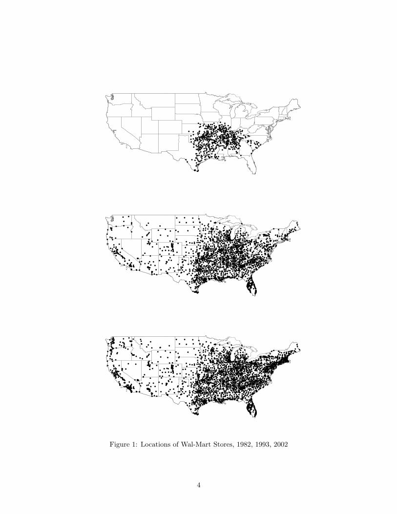

θ
φ
(Θ+φβT+1) (1-β)
T
t
t0 t1
T
θ
φ
(Θ+φβT+1) (1-β)
t
t0 t1
θ
(Θ+φβT+1) (1-β)φ
T
t
t0 t1
θ θ(1-β)
t0
t
θθ(1-β)
tt0
t
θ(1-β) θ
t0
t
Figure 4 Interpreting Regression Coefficients with Two Wal-Mart Coefficients
14
move slowly and do not return to their expected (trend-adjusted) level for several quarters
following any ldquoshockrdquo
In the presence of measurement error in prices the estimate of β is attenuated (biased
towards zero) and other point estimates including the estimate of θ are also biased If the
measurement error is solely or primarily due to errors in the process of collecting prices ndash eg
writing down a price of 079 when the true price is 097 ndash so that the errors are uncorrelated over
time we can address this problem by using pkjtminus2 the second lag of price to instrument for
pkjtminus1 Unless otherwise noted all the estimates shown below use this IV strategy to eliminate
(or at least reduce) the problem of measurement error
If measurement error is due to other causes ndash such as non-representative selection of retail
establishments in the price survey ndash twice-lagged price may not be a valid instrument For this
reason I experiment with a functional form that omits lagged price16
pjt = α + θWMopenjt +sum
j
γjcityj +sum
t
δtquartert +sum
j
τjtrendt + εjt (3)
Including lagged prices on the right-hand side of the regression is problematic for another
reason lagged price may be endogenous Endogeneity of lagged price could arise because the
error term εjt is not iid ndash for example if it follows an AR or MA process ndash in which case the
error term and lagged price will be correlated Like measurement error endogeneity of lagged
price would also yield biased estimates of Wal-Martrsquos effect in these regressions17
Instrumenting for lagged price with twice-lagged price as described above is a valid cor-
rection for endogeneity under some ndash but not all ndash conditions Specifically if the error term is
MA(1) an IV specification would be valid but if the error term is AR(1) it would not in that
case twice-lagged price (as well as any longer lag) would still be correlated with the error term
The alternative specification with no lagged price may be preferable under these conditions
(A completely exogenous instrument would be the best solution to this problem but none is
available as noted in footnote 16) While neither specification is perfect taken together the
16There is no available alternative instrument for lagged price A valid instrument needs to be correlated withlast quarterrsquos average price of a given good in a city after controlling for all the covariates but be uncorrelatedwith the error in measurement of lagged price
17The same problem would result if there is an omitted determinant of price which is correlated with laggedprice and is not captured by any of the other regressors in the model (A possible example could be entry ofanother large retailer if it depresses prices) Since the regression includes both city and time (quarter) fixedeffects to induce bias this omitted variable must vary across both time and cities and not follow a linear trendat the city level
15
two specifications tell a more complete story than either one tells alone
43 Measurement Error in Wal-Mart Data
I use instrumental-variables estimates to correct for two problems in the Wal-Mart variable
measurement error and endogeneity Inaccuracies in the directories and store lists combined
with the probabilistic method of assigning opening dates across quarters (and across years
over the period 1990-1993) lead to measurement error in the variable WMopenjt causing
attenuation bias in estimates of θ Endogeneity may also a problem even after controlling for
city-level trends if Wal-Mart entry is more likely in times of high (or low) prices relative to
the cityrsquos long-run trend In that case mean reversion alone will cause prices to fall (rise) and
the estimated coefficient θ may be spuriously negative (positive)
Measurement error in the Wal-Mart entry variable WMopenjt takes a particular form
while the entered cities are correctly identified the timing of entry may be incorrectly measured
due to errors in the directories The variable WMplanjt is also measured with error by
construction it represents the number of stores that would be open had stores always opened
in the order in which they were planned with the total number of stores opening each year is
held at its actual level and the distribution of opening dates across quarters assumed constant
ndash at 2001-04 levels ndash over the 20 year period
As long as the measurement errors in the two variables is classical and uncorrelated we can
use WMplanjt to instrument for WMopenjt The second assumption appears to be correct
it would be violated if for example stores in rural areas are completed faster than stores in
urban areas and also appear later in directories but this does not appear to be the case18
But measurement error is not classical the actual number of Wal-Mart stores in city j in
quarter t differs from the measured number by a number whose expected value is correlated
with the measured number (For example when the directories report zero Wal-Marts in town
the expected number of stores is some (small) positive number When the reported number of
Wal-Marts is one the actual number is usually either zero or one so the expected number is
less than one) This induces a slight bias in the instrumental-variables results reported here19
18There is no correlation between observable location characteristics and the time lag between the ldquoplanningdaterdquo and the opening date of a store
19Kane Rouse and Staiger [20] suggest a GMM estimator to address this problem Unfortunately due to thesize of the panel their solution is not computationally feasible in this setting While the bias could be large intheory in the static returns-to-schooling example of Kane Rouse and Staiger the bias is approximately 5 ofthe IV coefficient estimate The sign of this bias is indeterminate
16
The first-stage regression associated with Equation (1) is
WMopenjt = α + βpjtminus1 +sum
t
δtquartert + θWMplanjt +sum
j
τjtrendtj + εjt
Although the first-stage regression has a binary dependent variable I estimate the first-stage
by Ordinary Least Squares rather than a nonlinear model such as probit or logit Angrist and
Kreuger [2] caution against using a nonlinear first-stage model because unless it is exactly
right it will generate inconsistent second-stage coefficients A first-stage OLS specification in
contrast yields consistent second-stage estimates even if it is not exactly correct
This IV strategy can also correct for possible endogeneity of Wal-Martrsquos entry decision
Concerns about endogeneity have two dimensions Wal-Mart may select the cities it enters
non-randomly and it may choose the timing of entry non-randomly
The cross-sectional dimension (choice of cities) is very plausible for example Wal-Mart
may prefer to enter cities with less-competitive retail markets (hence higher pre-entry prices)
or with a larger fraction of search-savvy lower-middle income families (whose presence leads to
lower average retail prices see Frankel and Gould [14]) This concern is greatly mitigated by
the fact that Wal-Mart entry is observed in 162 of the 165 sample cities and the sample cities
are diverse with respect to all standard economic and demographic variables (see Table 3)
The timing dimension is important if Wal-Mart can schedule its entry to coincide with high
retail prices Under reasonable assumptions using WMplanjt to instrument for WMopenjt
can correct not only for measurement error but also for endogeneity in the timing of entry Of
course if there are omitted variables ndash if Wal-Martrsquos entry is correlated with other shocks to the
local retail market such as the entry or exit of other stores ndash in which case OLS estimates may
confound Wal-Martrsquos effect with price changes that happen for other reasons (Any omitted
city-specific variable that is either unchanged over this period or moves linearly will be captured
by the city fixed effects andor the city-specific trends in the model)
The identification strategy assumes that Wal-Mart plans its store entries well in advance
of entry and cannot accurately forecast exact market conditions (prices) at the time for which
entry is planned This assumption seems reasonable it can take a year and often longer to
get a property zoned acquire all the necessary building permits build and open a store for
business While Wal-Mart may want to enter any market at a time when prices are relatively
high ndash when potential profits as well as apparent benefit to consumers are highest ndash it cannot
17
predict the timing of high prices with any accuracy if the delay between planning and entry is
long enough The company may fine-tune opening dates based on current market conditions
but if the planning occurs sufficiently in advance ndash and prices are sufficiently flexible ndash then
planning dates can be treated as exogenous to retail prices at the time of Wal-Mart entry So
while the actual date of entry may be manipulated ndash moved forwards or delayed ndash to correspond
with ldquofavorablerdquo (high) price conditions the planned date of entry will be largely free of those
biases at least once we account for long-run differences in average prices across cities20
5 Results
51 OLS Results
Before proceeding to the IV results I show some results from OLS regressions of Equation (1)
Unless otherwise noted the specifications below use twice-lagged price as an instrument for
lagged price I use the term ldquoOLSrdquo to mean that the Wal-Mart variable WMopenjt is not
instrumented
Table 4 shows results from 10 separate OLS regressions Each row represents a separate
regression and shows the estimated coefficients θ (the instantaneous effect of Wal-Mart entry)
and β (the mean-reversionprice stickiness parameter) as well as the estimated long-run effect
of entry θ1minusβ Significance levels for the latter are given by the p-value from a (two-sided) Wald
test for H0 θ1minusβ = 0 So for example the average price of detergent is estimated to decline by
078 in the quarter following Wal-Mart entry and reach a decline of 386 asymptotically
OLS estimates of the price effect of Wal-Mart are negative for 9 of the 10 products (cigarettes
are the exception) and significant for three products ndash detergent shampoo and toothpaste
(although the latter is significant only at the 10 level) For these three products the estimated
short-run effect has a magnitude of 07-08 and the long-run magnitude of 35-4
The distinction between short- and long-run effects of Wal-Mart depend on the inclusion of
20A possible exception to this argument is if Wal-Martrsquos entry is correlated with the entry (or exit) of otherfirms If both the planning and the implementation of Wal-Mart entry coincides with that of other retailers ndashfor example if entry tends to be associated with the building of new ldquostrip mallsrdquo that bring additional storesndash coefficient estimates of the impact of Wal-Mart incorporate the impact of the ancillary entries By attributingthe joint causal effect to Wal-Mart we are assuming that the ancillary entries would not have occurred withoutWal-Martrsquos If this assumption is invalid ndash that is if other entries occur independently of but concurrently withWal-Martrsquos ndash the IV strategy described here would no longer be valid Anecdotal evidence suggests that otherstores enter (and exit) in response to Wal-Mart so that the instrument is valid Unfortunately data on thetiming of entry of other large retailers are not available so I cannot control directly for these
18
lagged price in the regression and on the validity of the IV correction for measurement error
in lagged price (and possibly for endogeneity as well) If lagged price is omitted from these
regressions the estimated effect of Wal-Mart (not shown) is negative for 8 of the 10 products
and statistically different from zero in four cases The statistically-significant coefficients range
from a 22 estimated decline in the price of shampoo (significant at the 10 confidence level)
to a 36 estimated decline in the price of detergent (significant at the 1 confidence level)
52 IV Results
Table 5 show instrumental variables estimates corresponding to Table 4 As expected where
measurement error is present almost all point estimates of θ are (absolutely) larger than the
OLS estimates Point estimates of Wal-Martrsquos effect show statistically significant short-run
declines of 15-3 in the prices of aspirin detergent Kleenex and toothpaste (with long-run
declines of 8-13) and marginally significant declines with similar magnitudes for shampoo
Only estimates of Wal-Martrsquos impact on the prices of cigarettes and pants are positive and
neither is significantly different from zero
Table 6 shows IV estimates of Equation (3) which omits the lagged price variable Qual-
itatively the results are extremely similar to the results in Table 5 The point estimates of θ
lie between the short- and long-run point estimates from the full model near their midpoint
Since results are qualitatively similar we can infer that uncorrected endogeneity of lagged price
is not seriously biasing the estimates of Wal-Martrsquos impact In these specifications the test
statistic for joint significance of the city-level trends increases by a factor of 10 or more exceed-
ing 500000 for all regressions (and reaching 50000000 for cigarettes) this suggests that there
is a strong relationship between price observations one quarter apart The model with lagged
price captures this relationship explicitly It also allows us to distinguish between the short-
and long-run effects of entry which this restricted model does not
Table 7 shows IV estimates of Equation (2) which allows for different effects of Wal-Mart
on prices in the short- and medium-runs (up to five years after entry) and the long-run The
coefficient φ represents the additional (positive or negative) change in price five years after
Wal-Mart entry Estimates of φ are generally small relative to θ it is positive large (2) and
significant for one product (toothpaste) With this one exception the estimates are broadly
similar to the ones shown in Table 5 in which only a single coefficient was estimated Long-run
effects are negative for all products except underwear
19
Table 4 OLS EstimatesProduct θ β θ
1minusβa
Aspirin -00025 07721 -00111(00041) (00189)
Cigarettes 00015 08350 0009
(00014) (00153) Coke -00035 07981 -00175
(00039) (00416) Detergent -00083 07946 -00406
(00032) (00206) Kleenex -00030 08043 -00152
(00024) (00248) Pants -00038 07556 -00156
(00040) (00238) Shampoo -00090 07932 -00437
(00035) (00232) Shirt -00057 07194 -00203
(00045) (00269) Toothpaste -00067 07899 -00319
(00040) (00225) Underwear 00006 07575 00026
(00057) (00235)Robust standard errors in parentheses (clustered by city)Regressions include city and quarter FE and city-specific price trendsF statistics from joint test for city level trends range form 20000-250000 significant at 10 significant at 5 significant at 1a Significance level from Wald test for H0 θ
1minusβ = 0
20
Table 5 IV EstimatesProduct θ β θ
1minusβa
Aspirin -00244 07685 -01053(00114) (00197)
Cigarettes 00019 08349 00112
(00034) (00153) Coke -00034 07981 -00169
(00092) (00415) Detergent -00193 07904 -00920
(00085) (00211) Kleenex -00156 08015 -00786
(00064) (00247) Pants 00015 07570 00062
(00108) (00232) Shampoo -00163 07920 -00784
(00093) (00233) Shirt -00008 07191 -00028
(00109) (00271) Toothpaste -00286 07846 -01327
(00111) (00228) Underwear -00016 07575 -00065
(00142) (00235)Robust standard errors in parentheses (clustered by city)Regressions include city and quarter FE and city-specific price trendsF statistics from joint test for city level trends range from 25000-450000 significant at 10 significant at 5 significant at 1a Significance level from Wald test for H0 θ
1minusβ = 0
21
This finding effectively rules out many possible scenarios among them the possibility that
while Wal-Martrsquos entry initially lowers prices prices rise again once competitors are driven out
of the market Instead Wal-Mart entry is associated with one relatively large price shock
which reverberates through the auto-regressive component21
53 Differential Impact of First and Later Entries
In the preceding regressions I consider only the effect of the first Wal-Mart store to enter a
city But many cities have more than one Wal-Mart store In 43 of sample cities ndash 70 of
164 ndash two or more store were open by the end of the sample period (Of these 36 cities had
two stores and 14 had three One city ndash Houston ndash had nine stores by the end of the sample
period)
To test whether the second Wal-Mart store has the same effect as the first I estimate
pjt = α + βpjtminus1 + θ1WMopenjt + θ2WMopen2jt
+sum
j
γjcityj +sum
t
δtquartert +sum
j
τjtrendtj + εjt (4)
where WMopenjt is as defined above and WMopen2jt equals 1 if there are at least two stores
in city j in quarter t22 Estimating θ1 and θ2 separately allows us to test directly whether the
second store has the same impact as the first
Estimation results are shown in Table 8 First-store effects are all of the same sign as in the
baseline specification (Table 5 with the statistically-significant effects (for aspirin detergent
Kleenex shampoo and toothpaste) all negative larger in absolute terms than in the baseline
specification The effect of the second store varies by product it is generally of a similar
magnitude but opposite sign to the first storersquos effect In the case of aspirin and toothpaste
it is positive and statistically significant (at 5 and 1 respectively)
Since θ1 estimates a once-and-for-all effect the joint (cumulative) effect of the first and
second stores is a function of both parameters To a first approximation (ignoring the time lag
between the first and second store openings) the joint effect of two stores is the sum of the
two coefficients θ1 and θ2 (The average lag between the first and second store openings in my
21Estimates of this specification without lagged price are qualitatively similar but magnitudes of the long-runeffect specified as θ + φ are slightly smaller in absolute terms
22I also define WMplan2jt which equals 1 if at least two Wal-Mart stores were planned to have opened in
city j by quarter t and use it as an instrument along with WMplanjt
22
sample for cities with more than one store is three years) This sum is generally very small
and tends to be negative but statistically insignificant
In specifications omitting the lagged dependent variable estimates of both θ1 and θ2 are
larger The sum θ1 + θ2 is statistically different from zero for two products ndash detergent and
Kleenex (at 10 and 5 significance respectively) in both cases the sum is negative
I also estimate a model in which the effect of Wal-Mart is linear in the number of stores
pjt = α + βpjtminus1 + θWMsopenjt +sum
j
γjcityj +sum
t
δtquartert +sum
j
τjtrendtj + εjt (5)
where WMsopenjt is the number (0-10) of Wal-Mart stores open in city j in quarter t (and
WMsplanjt the number of Wal-Mart stores planned to have opened in city j by quarter t
serves as the instrument) Across all products estimated θ coefficients (not shown) are small
(below 05 in absolute terms) and statistically indistinguishable from zero seven of the ten
are negative
54 City Size Effect
In this section I test the hypothesis that Wal-Martrsquos effect will be larger in cities with less
competitive retail markets Bresnahan and Reiss [4] and Campbell and Hopenhayn [5] among
others note that most models of imperfect competition predict smaller cities will have less
competitive retail markets but this prediction has been hard to test empirically
There is not a single obvious measure of city size The number of retail establishments in a
city is strongly correlated with population size in my sample the correlation coefficient between
the 1980 city population and the number of retail establishments the city had in 1982 is 098
The number of establishments does not increase one-to-one with population however larger
cities tend to have a larger absolute number of retail establishments but fewer establishments
per capita Small cities have disproportionately many small stores (Campbell and Hopenhayn
[5]) which are likely to be less efficient ndash and more expensive23
In Figure 5 I plot the number of retail establishments in 1982 against the number of re-
tail establishments per capita24 Outlier cities are individually labeled The figure highlights
23Dinlersoz [10] notes another difference between the organization of retail markets in small and large citieslarger cities have relatively fewer chain stores and more stand-alone stores which are likely to behave morecompetitively Counts of chains and stand-alone stores are not available for my sample
24Only the 142 sample cities with 1980 population above 25000 are included in the figure I use the 1980 Census
23
Table 6 IV Estimates without Lagged PriceProduct θ Product θ
Aspirin -00666 Pants 00274(00341) (00318)
Cigarettes 00153 Shampoo -00362
(00119) (00250) Coke 00110 Shirt 00194
(00282) (00291) Detergent -00589 Toothpaste -00863
(00274) (00310) Kleenex -00325 Underwear -00058
(00205) (00404)Robust standard errors in parentheses (clustered by city)Regressions include city and quarter FE and city-specific pricetrends F statistics from joint test for city level trends exceed500000 in all regressions significant at 10 significant at 5 significant at 1
0
0005
001
0015
002
0025
003
0 2000 4000 6000 8000 10000 12000 14000 16000 18000
Number of Retail Establishments 1982
Reta
il Es
tabl
ishm
ents
per C
apita
198
2
HoustonDallas
Philadelphia
Grand Junction CO
Hickory NCMissoula MT
Kingsport TNFlorence SCSarasota FL
San Diego
San Antonio
Phoenix00111
Figure 5 Total Retail Establishments vs Establishments per Capita (1982)
24
Table 7 IV Estimates with Different Short- and Long-Run EffectsProduct θ φ β θ+φmiddotβ21
1minusβa
Aspirin -00235 00011 07685 -01016(00103) (00081) (00198)
Cigarettes -00001 -00030 08359 -00013
(00031) (00029) (00159) Coke -00011 00032 07958 -00051
(00084) (00067) (00419) Detergent -00148 00062 07979 -00728
(00077) (00053) (00213) Kleenex -00129 00040 08001 -00645
(00061) (00033) (00246) Pants -00056 -00109 07503 -00226
(00101) (00070) (00249) Shampoo -00180 -00028 07888 -00854
(00087) (00068) (00233) Shirt -00009 -00002 07191 -00034
(00103) (00078) (00272) Toothpaste -00147 00203 07883 -00689
(00094) (00073) (00229) Underwear 00012 00043 07565 00051
(00125) (00090) (00237)Robust standard errors in parentheses (clustered by city)Regressions include city and quarter FE and city-specific price trendsF statistics from joint test for city level trends range from 25000-120000 significant at 10 significant at 5 significant at 1a Significance level from Wald test for H0 θ+φmiddotβ21
1minusβ = 0
25
Table 8 IV Estimates with Different First- and Second-Store EffectsProduct θ1 θ2 β
Aspirin -00355 00382 07660(00153) (00182) (00202)
Cigarettes 00033 -00050 08336
(00045) (00055) (00159) Coke -00051 00057 07983
(00124) (00167) (00415) Detergent -00249 00199 07899
(00108) (00133) (00213) Kleenex -00204 00171 08032
(00084) (00107) (00246) Pants 00037 -00078 07579
(00137) (00162) (00232) Shampoo -00209 00161 07921
(00121) (00148) (00234) Shirt -00075 00237 07164
(00147) (00203) (00268) Toothpaste -00453 00566 07787
(00166) (00209) (00236) Underwear -00040 00085 07568
(00176) (00226) (00235)Robust standard errors in parentheses (clustered by city)Regressions include city and quarter FE and city-specific price trendsF statistics from joint test for city level trends range from 40000-500000 significant at 10 significant at 5 significant at 1
26
the strong negative relationship between the number of retail establishments and their number
relative to population (the correlation coefficient is -037) Grand Junction Colorado (1980
population 28000) has the highest number of retail establishments per capita while Philadel-
phia (1980 population 17m) has the second-lowest (the lowest is in New Orleans with 1980
population of 560000) The horizontal line at 00111 indicates the median for this sample
While establishment breakdowns are not available at the city level approximately 10 of
retail establishments in the US in 1982 were clothing stores (SIC 5600) and 38 of retail
establishments were ldquodrug stores and proprietary storesrdquo (SIC 5910) (Both fractions declined
over the 1980s and 1990s each by approximately one percentage point) Therefore a city with
987 retail establishments (the median in my sample in 1982) had approximately 37 drugstores
ndash well within the intermediate range (between quintopolies and urban markets) considered by
Bresnahan and Reiss [4]
I estimate
pjt = α + βpjtminus1 + θ1WMopenjt middot lowj + θ2WMopenjt middot highj
+sum
j
γjcityj +sum
t
δtquartert +sum
j
τjtrendtj + εjt (6)
where low and high are indicator variables for cities with number of retail establishments per
capita in 1982 below and above the median (00111) respectively
Table 9 shows estimates of the coefficients of interest θ1 θ2 and β For nine of the ten
products θ2 is estimated to be negative (and statistically different from zero) with Wal-Martrsquos
short-run effects estimated to be between 2-4 θ1 is never statistically different from zero
The difference between these coefficients is statistically significant for shampoo at the 10
significance level for shirt at the 5 significance level and for detergent and Coke at the 1
level Long-run effects are magnified by β and range from 10-20 for small cities (cities with
many retail establishments per capita) long-run effects for large cities (with few establishments
per capita) are never statistically different from zero25
population rather than 1982 population estimates to compute the per-capita number of retail establishments25When lagged price is omitted from the regressions estimates of θ1 are negative for 6 of the 10 products
and estimates of θ2 are negative for 7 of the 10 products In contrast to the main specification however θ2 isstatistically significant in only three cases for detergent the estimated price decline for cities with many retailestablishments per capita is 11 (significant at the 1 level) for toothpaste it is 95 (significant at the 5level) and for shampoo it is 6 (significant at the 10 level) The estimate of θ1 is significant (at the 10 level)in one case for the price of a shirt where it implies a price increase of 6 due to Wal-Mart entry
27
As a robustness check I also estimate a model in which I interact the number of retail
establishments per capita in 1982 (a continuous variable) with the Wal-Mart variable (The
equation also includes a main Wal-Mart effect city fixed effects prevent estimation of a main
1982-establishments-per-capita effect) The interaction term is negative in 9 of 10 regressions
(not shown) again indicating that Wal-Martrsquos negative price effect is larger in cities with many
establishments per capita For three products ndash Coke shampoo and shirt ndash the interaction
term is statistically significant at the 10 level and it is significant at the 5 level for detergent
Interestingly when I separate the cities in the sample into ldquosmallrdquo and ldquolargerdquo using alter-
native criteria ndash such as 1980 city population or 1982 absolute number of retail establishments
ndash the two coefficients (θ1 and θ2) are never statistically different from one another26 This sug-
gests that the number of establishments per capita may be a better measure of competitiveness
than the absolute number of retail establishments in a city However the strong correlation
between population absolute number of retail establishments and number of establishments
per capita prevents us from drawing any definitive conclusions on the main cause of the vari-
ation in Wal-Martrsquos impact when I allow for simultaneous interactions of Wal-Mart entry
with log population and retail establishments per capita none of the interaction coefficients are
statistically different from zero
6 Discussion and Conclusion
This paper tests the hypothesis that Wal-Mart entry leads to lower average retail prices in the
markets it enters Using a unique panel data set that combines average retail prices for 10
specific goods and a complete time-series of Wal-Mart store locations I estimate the effect of
Wal-Mart entry on prices I find that for many items typically sold in drugstores such as aspirin
and shampoo average prices decline following Wal-Mart entry This decline is economically
large ndash 15-3 in the short run and four times as much in the long run ndash and statistically
significant
These findings are in line with other price surveys In April 2002 UBS Warburg collected
prices of 100 grocery and non-grocery items in 4-5 grocery stores in each of four large markets
Sacramento a city with no Wal-Mart presence and Las Vegas Houston and Tampa each of
26In a model with continuous interaction term with log population Wal-Martrsquos effect varies very little withpopulation only in two cases is the coefficient different from zero at the 5 confidence level
28
which had at least one Wal-Mart Supercenter Their study found that Wal-Martrsquos prices were
17-39 lower than competitorsrsquo prices in the three ldquoWal-Mart citiesrdquo and that average prices
at other grocery stores were 13 lower in the Wal-Mart cities than in Sacramento (Currie
and Jain [9]) I repeated Currie and Jainrsquos analysis using a subset of 24 drugstore products
from their data set comparable to the ACCRA products Tylenol Pepto Bismal shampoo
deodorant feminine hygiene items soap toothpaste detergent and Coke For these items
Wal-Martrsquos prices were 23 lower on average than competitorsrsquo prices in the Wal-Mart cities
Competitorsrsquo prices in Wal-Mart cities were lower than Sacramento prices for most but not all
items on average drugstore prices were 15 lower in Wal-Mart cities Of course these numbers
should be interpreted cautiously due to the cross-sectional nature of the data the small number
of cities included and the exclusive reliance of the sample on grocery store prices
Since figures on profit margins for Wal-Mart competitors in the entered markets are not
available I use Census data to assess the economic significance of these estimates The Census
Bureaursquos annual series ldquoCurrent Business Reports Annual Benchmark Report for Retail Trade
and Food Servicesrdquo provides data on average gross margins (roughly the retail price markup
over wholesale price) by retail sub-sector from 1986-2001 (US Census Bureau [28] and [29])
Gross margins do not account for any other costs such as labor rent or capital inputs and
should not be mistaken for profit margins Apparel stores have gross margins above 40
on average meaning that wholesale costs account for under 60 of the retail prices charged
by apparel stores on average Drugstores have margins of 25-30 on average27 Using this
benchmark a decline of 5 in the price of some drugstore items can be interpreted as a decline
of 15-20 in the gross margin of drugstores28
In interpreting the point estimates of Wal-Martrsquos effect several caveats are in order
First the average-price effect masks a large amount of intra-market variation in competitive
response to Wal-Mart entry Because the ACCRA data cannot be disaggregated to the store
27The exact definition of these industries changes halfway through the sample due to the shift from SIC toNAICS For the period 1993-1998 when both SIC and NAICS-based figures are available the implied marginsare very similar
28An alternative more detailed benchmark is provided by the University of Chicago Graduate School ofBusiness study of Dominickrsquos Finer Foods (DFF) in the Chicago metropolitan area Over the period 1989-1994the GSB collected scanner data including gross margins from Dominickrsquos for thousands of individual itemsThese data are available on-line athttpgsbwwwuchicagoedukiltsresearchdbdominicksindexshtml
and are described in detail in Peltzman [24] and Chevalier Kashyap and Rossi [8] Several of the items includedin this analysis are also included in the DFF database The average gross margin on items classified as ldquodrugstoreproductsrdquo in this study is 12
29
level it is impossible to estimate the distribution of responses But theory suggests that stores
selling the closest substitutes to Wal-Mart ndash for example those that are located near Wal-Mart
or that are similar on other dimensions ndash will have the most elastic price responses to Wal-Mart
entry Stores located far from Wal-Mart are likely to have very small price responses because
their clientelesrsquo cross-price elasticity of demand will be low
A related problem is that Wal-Mart stores may be included in ACCRArsquos surveys If Wal-
Martrsquos prices are lower on average than other storesrsquo (Currie and Jain [9] Hausman and
Leibtag [17]) then it is impossible to distinguish in my results between Wal-Martrsquos direct
effect on average prices and the more interesting indirect effect due to competitive pressures
on other stores ACCRArsquos explicit instruction to sample only retailer that cater to the upper
quintile of the income distribution mitigates this concern because it reduces the probability
that Wal-Mart will be sampled It also reduces the probability that many of Wal-Martrsquos direct
competitors ndash other discount retailers ndash will be in the sample The absence of discount stores
and more generally the over-sampling of stores that cater to the upper quintile biases my
estimates against finding any effect of Wal-Mart29
Third ACCRA weights all establishments equally in computing average prices If Wal-
Martrsquos prices are indeed lower than their competitorsrsquo prices and consumers respond to Wal-
Mart entry by shifting demand from incumbent establishments to Wal-Mart the effect on the
unweighted price average estimated here will be lower than the effect on the effective average
price paid by consumers (properly weighted) This issue is important but require additional
data ndash on quantities purchased ndash to resolve 30
Pricing strategies that vary by type of store may bias the result in the opposite direction
Many drug- and grocery stores use so-called ldquoHigh-Lowrdquo pricing so that an item alternates
between a high ldquoregularrdquo and a low ldquosalerdquo price while Wal-Mart uses ldquoevery day low pricingrdquo
which is lower on average than competitorsrsquo prices but is rarely the lowest price in the market
For non-perishable goods such as the ones considered in this paper consumersrsquo ability to buy in
bulk during sales means that the unweighted average price computed by ACCRA under-weights
sale prices If Wal-Martrsquos entry pushes down the ldquohighrdquo (regular) price charged by incumbents
29This effect is probably strongest for clothing where there is a wide variance in store attributes even if theproduct is relatively homogeneous This may explain why my estimates of Wal-Martrsquos effect on clothing pricesare consistently nil
30Hausman and Leibtag [17] raise similar points in their discussion of Wal-Martrsquos effect on aggregate inflationthey use household-level scanner data to estimate these biases in the CPI and find them to be quite large
30
but does not affect either the probability of a sale or the sale price the estimated impact of
Wal-Mart will be much larger than its properly-weighted effect Quantity data are needed in
order to address this issue as well
Finally the products selected by ACCRA are not a random sample For the purpose of
price comparison across cities ACCRA selected well-known national brands for its price survey
these itemsrsquo prices may not be representative of ldquotypicalrdquo drugstore and clothing prices If the
difference between Wal-Martrsquos and other storesrsquo prices is greater for national brands than for
local and ldquostorerdquo brands ndash perhaps because national brands have higher margins ndash the estimated
effect of Wal-Mart will be biased away from zero We do not observe that margins are higher
on national brands in the Dominickrsquos price data if anything the brands considered here have
lower margins than average in their categories (eg margins for Colgate and Crest toothpaste
are lower than the average toothpaste margin)
Despite these caveats the estimated effect of Wal-Mart on the prices of several products
considered here are strong and robust Wal-Martrsquos effect is strongest for products traditionally
sold in drugstores and weakest or absent for cigarettes and Coke (sold in many outlets
including convenience stores) and clothing This result is intuitively appealing since (with the
relatively recent exception of grocery stores) Wal-Mart competes most directly with drugstores
The estimated effects are also strongest for cities with a large number of retail establishments
per capita consistent with the intuition that Wal-Martrsquos entry brings lower prices to consumers
in relatively small cities where establishments tend to be smaller and retail environments less
competitive than in large cities
31
Tab
le9
IVE
stim
ates
byR
etai
lE
stab
lishm
ents
per
Cap
ita
Pro
duct
θ 1θ 2
θ 1=
θ 2a
βθ 1
1minus
βb
θ 21minus
βb
θ 11minus
β=
θ 21minus
βa
Asp
irin
-00
207
-00
234
002
020
7625
-00
873
-00
986
002
04(0
014
1)(0
015
9)(0
887
1)(0
022
5)(0
886
8)
C
igar
ette
s0
0006
-00
010
007
140
8324
000
36-0
005
90
0715
(00
047)
(00
045)
(07
897)
(00
164)
(07
895)
Cok
e0
0174
-00
296
9
5615
080
95
0
0912
-01
553
7
4456
(00
114)
(00
121)
(00
024)
(00
431)
(00
072)
Det
erge
nt-0
000
3-0
045
8
928
840
7814
-00
015
-02
093
10
054
(00
106)
(00
122)
(00
028)
(00
228)
(00
019)
Kle
enex
-00
063
-00
221
2
2595
079
64
-0
031
1-0
108
5
227
55(0
007
3)(0
009
3)(0
135
0)(0
025
4)(0
133
7)
Pan
ts0
0139
-00
042
113
120
7651
005
90-0
017
91
1490
(00
136)
(00
131)
(02
893)
(00
264)
(02
856)
Sham
poo
-00
020
-00
306
3
4004
079
27
-0
009
8-0
147
4
341
06(0
012
5)(0
011
9)(0
067
3)(0
024
1)(0
066
9)
Sh
irt
001
78-0
029
05
7983
070
56
0
0606
-00
986
607
40(0
012
8)(0
016
9)(0
017
3)(0
030
4)(0
014
9)
Too
thpa
ste
-00
177
-00
360
0
9560
078
26
-0
081
6-0
165
4
097
63(0
014
5)(0
014
2)(0
329
9)(0
024
5)(0
324
8)
U
nder
wea
r-0
023
30
0170
256
690
7643
-00
988
007
222
7226
(00
197)
(00
184)
(01
114)
(00
250)
(01
012)
Rob
ust
stan
dard
erro
rsin
pare
nthe
ses
(clu
ster
edby
city
)R
egre
ssio
nsin
clud
eci
tyan
dqu
arte
rFE
and
city
-spe
cific
pric
etr
ends
F
stat
isti
csfr
omjo
int
test
for
city
leve
ltr
ends
rang
efr
om20
000
-200
000
si
gnifi
cant
at10
sign
ifica
ntat
5
si
gnifi
cant
at1
aF
stat
isti
c(p
-val
ue)
from
test
for
H0
θ1
=θ 2
bSi
gnifi
canc
ele
velfr
omW
ald
test
for
H0
θ
1minus
β=
0
32
References
[1] American Chamber of Commerce Research Association ACCRA Cost of Living Index
Manual (2000)
[2] JD Angrist AB Krueger Instrumental Variables and the Search for Identification From
Supply and Demand to Natural Experiments Journal of Economic Perspectives 15 (2001)
69-85
[3] E Basker Job Creation or Destruction Labor-Market Effects of Wal-Mart Expansion
Review of Economics and Statistics 87 (2005 forthcoming)
[4] TF Bresnahan PC Reiss Entry and Competition in Concentrated Markets Journal of
Political Economy 99 (1991) 977-1009
[5] JR Campbell HA Hopenhayn Market Size Matters Federal Reserve Bank of Chicago
Working Paper 2003-12 (2003)
[6] Chain Store Guide Directory of Discount Department Stores Business Guides Inc New
York 1979-1982 1987-1993
[7] Chain Store Guide Directory of Discount Stores Business Guides Inc New York 1983-
1996
[8] JA Chevalier AK Kashyap PE Rossi Why Donrsquot Prices Rise During Periods of Peak
Demand Evidence from Scanner Data American Economic Review 93 (2003) 15-37
[9] N Currie A Jain Supermarket Pricing Survey UBS Warburg Global Equity Research
publication 2002
[10] EM Dinlersoz Firm Organization and the Structure of Retail Markets Journal of Eco-
nomics and Management Strategy 13 (2004) 207-240
[11] A Edgecliffe-Johnson A Friendly Store from Arkansas Financial Times June 19 1999
[12] JM Feiner AH DrsquoAndraia J Black CE Jones RJ Konik Wal-Mart Encyclopedia
X Building a Global Brand Lehman Brothers New York 2001
[13] S Foley T Mahmood WalMart Stores Inc Harvard Business School Case Study 9-794-
024 (1996)
33
[14] DM Frankel ED Gould The Retail Price of Inequality Journal of Urban Economics 49
(2001) 219-239
[15] P Ghemawat Wal-Mart Storesrsquo Discount Operations Harvard Business School Case Study
9-387-018 (1989)
[16] P Ghemawat G Friedman Wal-Mart in 1999 Harvard Business School Case Study N9-
799-118 (1999)
[17] J Hausman E Leibtag CPI Bias from Supercenters Does the BLS Know that Wal-Mart
Exists National Bureau of Economic Research Working Paper 10712 (2004)
[18] J Hopkins Wal-Martrsquos Influence Grows USA Today January 29 2003
[19] H Hotelling Stability in Competition Economic Journal 39 (1929) 41-57
[20] TJ Kane CE Thomas Rouse D Staiger Estimating Returns to Schooling When School-
ing is Misreported Princeton Industrial Relations Section Working Paper 419 (1999)
[21] The Lex Column The Wal-Mart Way Financial Times February 19 2003
[22] McKinsey Global Institute US Productivity Growth 1995-2000 Understanding the Con-
tribution of Information Technology Relative to Other Factors MGI Washington DC
2001
[23] DC Parsley S-J Wei Convergence to the Law of One Price without Trade Barriers or
Currency Fluctuations Quarterly Journal of Economics 111 (1996) 1211-1236
[24] S Peltzman Prices Rise Faster than They Fall Journal of Political Economy 108 (2000)
466-502
[25] JF Reinganum A Simple Model of Equilibrium Price Dispersion Journal of Political
Economy 87 (1979) 851-858
[26] B Saporito Can Wal-Mart Get Any Bigger Time January 13 2003
[27] US Census Bureau County and City Data Book US Government Printing Office Wash-
ington DC various years a
[28] US Census Bureau Current Business Reports Annual Benchmark Report for Retail
Trade Washington DC various years b
34
[29] US Census Bureau Current Business Reports Annual Benchmark Report for Retail
Trade and Food Services Washington DC various years c
[30] SS Vance RV Scott Wal-Mart A History of Sam Waltonrsquos Retail Phenomenon Twayne
Publishers New York 1994
[31] Wal-Mart Stores Inc Annual Report 1971-2001
35
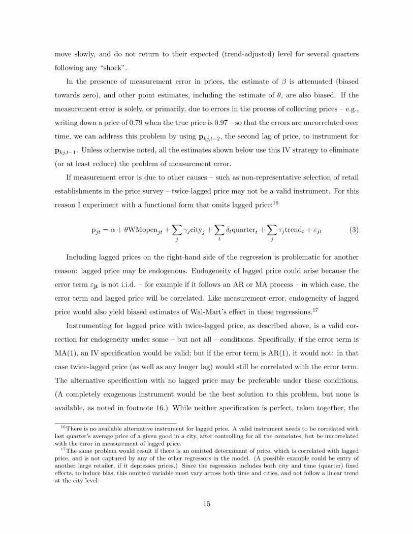
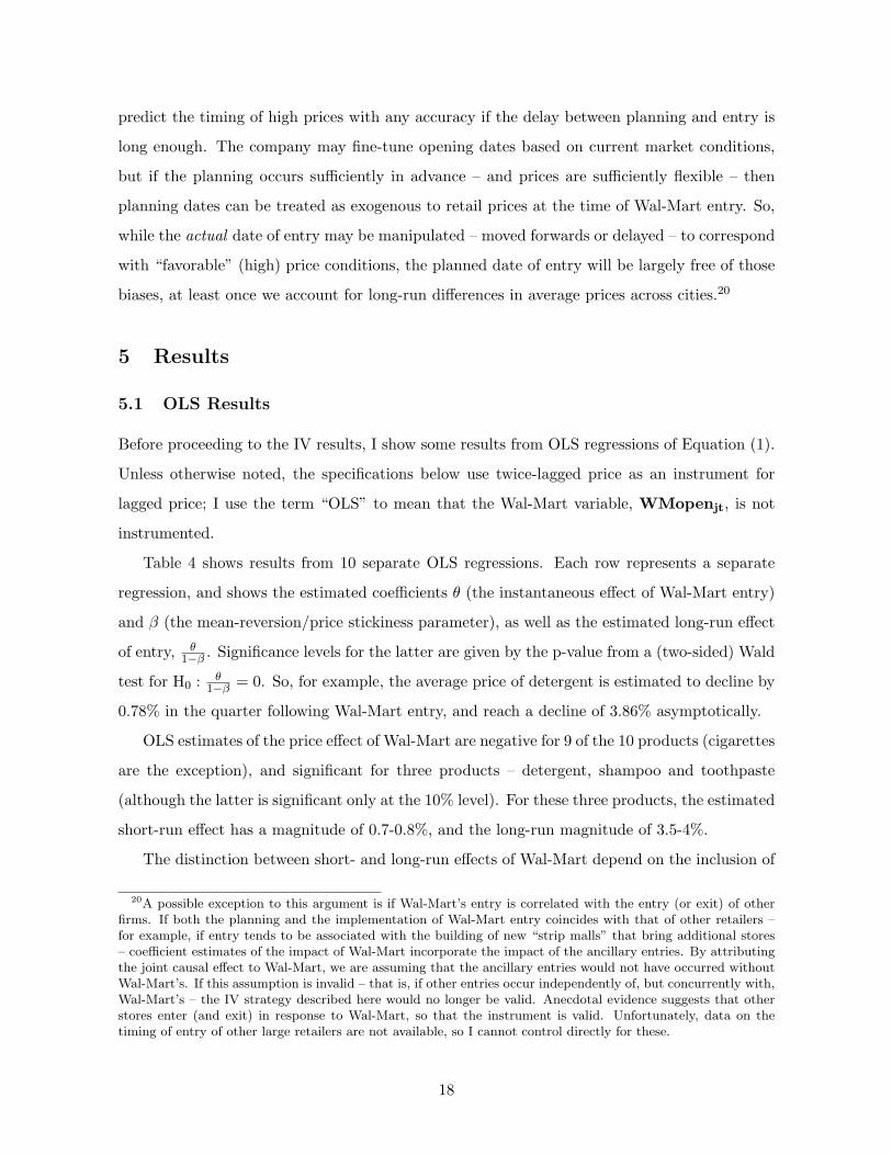
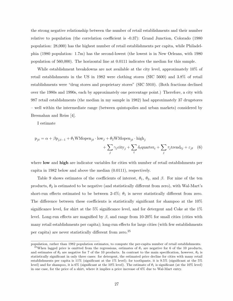
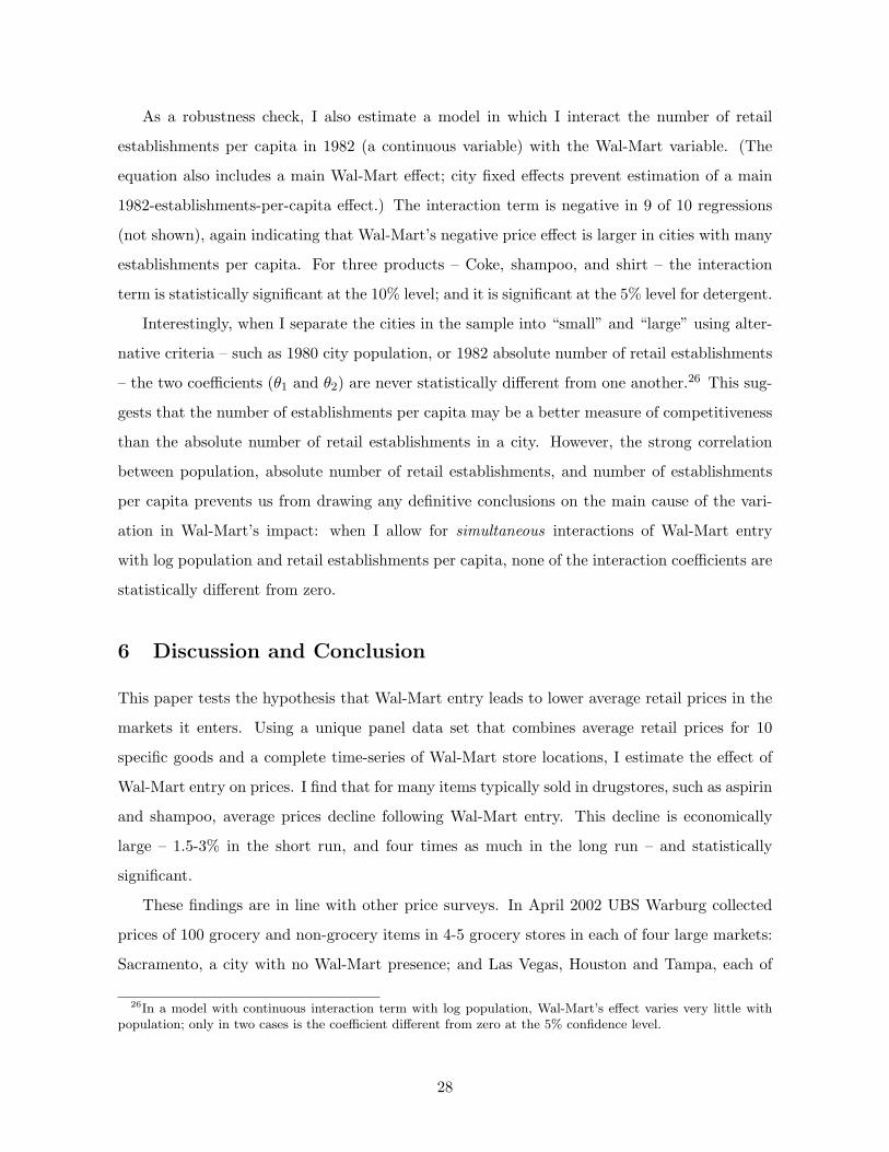
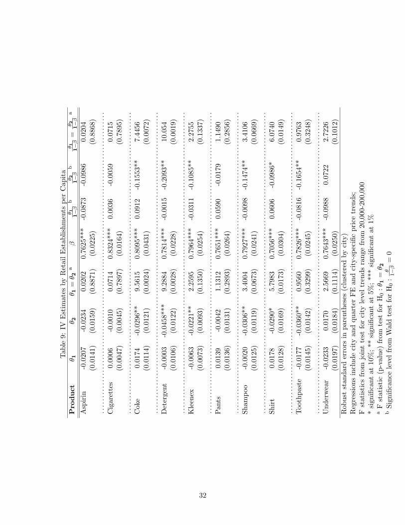

[29] US Census Bureau Current Business Reports Annual Benchmark Report for Retail
Trade and Food Services Washington DC various years c
[30] SS Vance RV Scott Wal-Mart A History of Sam Waltonrsquos Retail Phenomenon Twayne
Publishers New York 1994
[31] Wal-Mart Stores Inc Annual Report 1971-2001
35