Self-Optimizing Control of the Kaibel Distillation

Column

Håkon Olsen

December 19, 2005

Abstract

The minimum singular value method for finding optimal controlled variablesis introduced. The method is applied to control structure design for a four-product Kaibel distillation column, which is a mass and heat integrated sep-aration column. The selection method is based on steady-state optimization.It is shown how this can be done, using the commercial process simulatorHysys v3.2.

KEYWORDS : Control Structure Design, Optimization, Convexity.

Contents

1 Background 41.1 The Kaibel Distillation Column . . . . . . . . . . . . . . . . . 41.2 The Physics of Distillation . . . . . . . . . . . . . . . . . . . . 5

1.2.1 The Effect Changing the Flow Inputs . . . . . . . . . . 61.3 Self-Optimizing Control . . . . . . . . . . . . . . . . . . . . . 6

1.3.1 Selection of controlled outputs . . . . . . . . . . . . . 61.4 Mathematical Background . . . . . . . . . . . . . . . . . . . . 8

1.4.1 Convexity . . . . . . . . . . . . . . . . . . . . . . . . . 81.4.2 A Formal Definition of Convexity . . . . . . . . . . . . 91.4.3 Numerical Optimization Algorithms . . . . . . . . . . 10

1.5 Computational Issues . . . . . . . . . . . . . . . . . . . . . . . 121.5.1 Distillation Models . . . . . . . . . . . . . . . . . . . . 121.5.2 Thermodynamic Models . . . . . . . . . . . . . . . . . 13

2 Control Structure Selection 152.1 Model of the Kaibel Column . . . . . . . . . . . . . . . . . . . 152.2 Nominal Operating Point . . . . . . . . . . . . . . . . . . . . 16

2.2.1 Characterization of the Optimization Problem . . . . . 162.3 Calculation of Span . . . . . . . . . . . . . . . . . . . . . . . . 17

2.3.1 Problems in the calculation . . . . . . . . . . . . . . . 182.4 The Scaled Gain Matrix and Optimal Selection . . . . . . . . 18

2.4.1 Loss Calculations . . . . . . . . . . . . . . . . . . . . . 202.5 Startvalue Correction for Optimization . . . . . . . . . . . . . 21

3 Control Configuration 243.1 Control with Four Temperature Measurements . . . . . . . . 243.2 Sensitivity Analysis . . . . . . . . . . . . . . . . . . . . . . . . 253.3 Results from the Singular Value Rule . . . . . . . . . . . . . . 26

4 Concluding Remarks 29

A Bracketing Calculations 30

B Software Descriptions 31

2

Preface

This report is the culmination of my project work, as part of the special-ization in process systems engineering at the Department of Chemical Engi-neering at the Norwegian University of Science and Technology (NTNU).

The aim of the project was to find a self-optimizing control structure forthe Kaibel distillation column, which is a column with a dividing wall, whichmakes it possible to separate up to four components in one column shell.

3

Chapter 1

Background

1.1 The Kaibel Distillation Column

The Kaibel distillation column was introduced by Gerd Kaibel at BASF in1987. The Kaibel column is a heat and mass integrated separation process,with potential for large savings in capital cost, energy requirement and plotspace compared to the conventional sequential distillation for multicom-ponent separations. In sequential distillation one needs three columns toseparate four components. Up to 40% savings in plot space has been re-ported, and up to 25% and 35% respectively for investment and operatingcost [Wenzel and Röhm, 2003].

Heat and mass integration can be achieved both in a dividing-wall imple-mentation and when the prefractionator and main tower are built in separateshells. A laboratory column has been built at the Department of ChemicalEngineering, NTNU, to do pilot plant experiments, and this column has beenbuilt with two shells. This would not be the best solution in an industrialapplication, when investment costs are important, but the energy savingswill be the same, assuming adiabatic operation.

A conceptual model of the Kaibel column is shown in figure 1.1. On theleft hand side, the prefractionator is shown, where the 4-component mixtureis split into two fractions; one light and one heavy. On the right hand side,the main separation tower is shown, where the two fractions are split intotheir respective components. There is only one reboiler and one condenserfor such a column.

BASF has implemented several dividing-wall columns in production scale.A simulation structure for design of such columns is given by Kaibel [Kaibel et al., 2004].Kaibel also mentions the control of such columns at BASF, and the controlobjective is most often to maintain the product balance (steady-state op-eration) and the given quality constraints. The control loops at BASF aredesigned and implemented without dynamic simulations.

For the control of the column, there are 6 steady-state degrees of free-

4

Figure 1.1: Schematic of a Kaibel distillation column

dom: reflux and boil-up, splits of internal streams and two product streams.In the analysis to follow, two of these (boil-up and vapor split) are kept con-stant, and the remaining 4 degrees of freedom are available to the controlsystem. The simulation is based on molar flows, but the real system will becontrolled based on volume flow. Assuming a nearly constant compositionprofile (molar mass profile), these are one-to-one related variables.

1.2 The Physics of Distillation

The separating agent in distillation is energy, supplied to the distillation col-umn in the reboiler. Continuous distillation is a staged separation process,and vapor and liquid phases are contacted at each stage, where equimolardiffusion occurs. The driving forces for the diffusion are entropic in nature,and with sufficient contact time and interface between the phases will even-tually reach equilibrium at each stage. In real distillations the process is notat equilibrium, but the equilibrium model serves as a good conceptual modelfor understanding the behavior of the distillation process. The underlyingassumption is that two un-equilibrated streams entering a typical stage, havea residence time at the stage which is much larger than the necessary contacttime for equilibrium to be reached through diffusion.

For control purposes it is interesting to know how different manipulablevariables affect the process. First of all, the measurements normally ac-cessible to control are temperature measurements. The temperature profileof a distillation column is coupled to the concentration profile through thethermodynamics. Concentrations are hard to measure directly, and the mea-

5

surement is slow. The link between the temperature measurements and theproduct concentrations is established as an empirical model.

The pressure in a distillation column is set such that the condenser andreboiler can work with the utilities available. In most cases the pressure iskept constant (often atmospheric), but it can also be a controllable prop-erty. This can be practical for example when operating close to the utilityconstraints, because of changes in ambient temperature. Increasing the pres-sure increases the condenser temperature, but at the same time the reboilertemperature increases.

1.2.1 The Effect Changing the Flow Inputs

Often in distillation, the internal flows, reflux and boil-up, are used as controldegrees of freedom. In a two-product multicomponent distillation column,the effect of changing an internal flow on the concentration profile is to movethe whole profile; one product tends to get purer, whereas the other gets lesspure [Skogestad, 1997]. However, the effect of changing the external flowsis much larger, if one draws a lot more in the top stream as there is lightcomponent in the feed, it is obvious that the product purity will be lower.The use of external streams as controlled variables is limited, because theyare often needed in order to stabilize levels in the reboiler and reflux drum.

1.3 Self-Optimizing Control

When operating a chemical process, there is usually some optimal operatingpoint, and it is economically imperative to stay close to this operating point.This point is however dependent on process conditions, and may move inthe state-space due to disturbances on the process. The primary controlobjective is related to profits, and thus the selection of controlled variablesshould reflect this. In other words; the selection of the best control structureis a question of optimization; a structure should be selected so that the loss,L = J(u, d)−J∗(d) is minimized, where J is an objective function describingthe operational objective, and J ∗(d) is the optimum for a given disturbanced.

Skogestad and Postlethwaite [Skogestad and Postlethwaite, 2005] definethe concept of self-optimizing control the following way:

Definition 1 (Self-Optimizing Control) Self-optimizing control is whenan acceptable loss can be achieved with constant set-points, without the needfor reoptimization when disturbances occur.

1.3.1 Selection of controlled outputs

The method used for selecting optimal controlled variables is a local opti-mization method. The loss is defined as above. Make the following assump-

6

tions:

• the cost function J is smooth.

• the optimization problem is unconstrained, i.e., active constraints arealready controlled at their optimal values.

• the dynamics of the process can be neglected when evaluating the cost.

• the control problem is square (the number of controlled outputs equalsthe number of manipulated variables).

Then, a second order approximation to the objective function is made bya Taylor expansion around the optimal operating point (where ∆u = u−u∗,etc.):

J(u, d) = J∗(d) + (∇uJ∗)T ∆u +1

2(∆u)T (∇2

uJ∗)∆u (1.1)

Then, the loss can be written the following way:

L = J(u, d) − J∗(d) =1

2(∆u)T (∇2

uJ∗)∆u (1.2)

To analyze how the loss inflict on the objective function by the nonop-timal inputs ∆u affects the output selection, assume a steady-state linearmodel is available,

z = Gu + Gdd (1.3)

where G and Gd are steady-state gain matrices for the inputs and distur-bances respectively. Assuming that G is non-singular and focusing on theinput-output behavior:

∆u = G−1∆z (1.4)

Equation (1.4) together with (1.2) yields

L =1

2(G−1∆z)T (∇2

uJ)(G−1∆z) =1

2(∆z)T G−T Juu(G−1∆z) (1.5)

Now, defining a mapping of z through the loss model;

z := J1/2uu G−1∆z (1.6)

The loss minimization can be expressed as a norm minimization problem;

L =1

2‖z‖2

2 (1.7)

The control error can be separated in two terms; the implementationerror and the optimization error due to the non-optimal operating point. The

7

optimization error can be estimated as the worst-case variation in solutions tothe optimization problem with varying disturbances. Let r be the referencepoint for the controlled variable z. Then the error can be expressed:

e = z − z∗ = z − r︸ ︷︷ ︸

I

+ r − z∗︸ ︷︷ ︸

eopt

(1.8)

where I is the implementation error and eopt the optimization error. Withintegral action in the controller, there is no setpoint tracking error, and theimplementation error is basically the measurement error.

From (1.5), it is easily seen that, to obtain good control, one should seekcontrolled variables such that:

• G−1 is small, that is, the gain should be high.

• eopt should be small; zopt should be insensible to disturbances.

• G should be well conditioned.

MIMO Systems: Minimum Singular Value

Assume that the optimal variation in the outputs is uncorrelated, that is, theworst-case deviation ‖z − z∗‖ = 1 can occur. Assume also that the inputsare scaled such that a given deviation ∆ui has a similar effect on the costfunction J for all inputs, that is, the Hessian is a constant α times a unitarymatrix, where α = σ(Juu). Then the norm of the augmented error, z, is

‖z‖ = σ(J1/2uu G−1), and the worst-case loss is;

max‖z−z∗‖≤1

L =1

2σ2(α2G−1) =

α

2

1

σ2(G)(1.9)

From equation (1.9) it is apparent that controlled variables should be chosento maximize the minimum singular value.

1.4 Mathematical Background

1.4.1 Convexity

Convexity is a very important property of an optimization problem. A scalar-valued function is convex in a point if its second derivative in the pointis positive. If this holds for all points in the domain of the function, thefunction is itself called convex. A minimizer for a convex function is a globalminimizer, because there exists a unique minimum. An example of a convexfunction is shown in figure 1.2. A non-convex function is shown in figure 1.3,such a function may have several minima, and the global one is thereforehard to find.

8

−5 0 5−1

0

1

2

3

4

5

x

f(x)

Figure 1.2: A convex function

−5 0 5−3

−2

−1

0

1

2

3

x

f(x)

Figure 1.3: A non-convex function

1.4.2 A Formal Definition of Convexity

Definition 2 (Convex Set) A set S ∈ Rn is called convex if a straight line

segment connecting any two points in S lies entirely within S. Formally, forany two points (x, y) ∈ S: αx + (1 − α)y ∈ S,∀α ∈ [0, 1].

Definition 3 (Convex Function) A function f is called convex if its do-main is a convex set as defined in definition 2, and if for any two points(x,y) in the domain of f, the graph of f lies below the straight line connecting(x,f(x)) to (y,f(y)) in the (n+1)-dimensional space R

n+1. That is, we have∀α ∈ [0, 1]:

f(αx + (1 − α)y) ≤ αf(x) + (1 − α)f(y)

Convex Programming

Convex programming is a term used for the solution of a special class ofconstrained optimization problems, where the objective function is convex,the equality constraints are linear and the inequality constraints are concave.This is usually not the case in process optimization, because the thermody-namic equilibrium is mostly described by nonlinear functions, and these arethen equality constraints for the optimization problem.

9

1.4.3 Numerical Optimization Algorithms

The optimization methods utilized in this work are local. The most popularclass of local optimization methods is the quasi-Newton approach. Assumewe have an unconstrained nonlinear problem. For the quasi-Newton ap-proach, this objective function J(p) is approximated by a quadratic functionmk(p), where p is the vector of free variables. J is assumed to be a real-valuedscalar function. The quadratic approximation is given by;

mk(p) = Jk + ∇JTk p +

1

2pT Bkp (1.10)

where B is some positive definite matrix, which is updated on every iteration.This model is convex and quadratic, and its minimizer, pk can be givenexplicitly as;

pk = −B−1

k ∇Jk (1.11)

The minimizer given in (1.11) is used as the search direction, and the newiterate is then

xk+1 = xk + αkpk (1.12)

where the step length must satisfy the Wolfe conditions. The Wolfe condi-tions guarantee a step length that yields sufficient decrease of the objectivefunction, assuming convexity The following must be fulfilled:

J(xk + αkpk) ≤ J(xk) + c1αk∇Tk pk

∇J(xk + αkpk)T ≥ c2∇JT

k pk

where 0 < c1 < c2 < 1. The difference between this method and an exactNewton method, is that an approximation of the Hessian is used instead ofthe true one.

The update formula for the Hessian approximation should satisfy someimportant criteria: it must be positive definite and symmetric. One of themost popular update formulas, is the BFGS formula, here simply stated forreference.1 For details about the BFGS update, see [Nocedal and Wright, 1999]For convenience of notation the following vectors are defined:

sk := xk+1 − xk (1.13)

yk := ∇Jk+1 −∇Jk (1.14)

Then the BFGS formula can be written as:

Hk+1 = (I − ρkskyTk )Hk(I − ρkyks

Tk ) + ρksks

Tk (1.15)

1BFGS is an abbreviation for Broyden, Fletcher, Goldfarb and Shanno, the discoverers

of the formula

10

where ρ = 1

yTk

skand Hk is the inverse of the Hessian approximation:

Hk = B−1

k

The quasi-Newton BFGS method applies directly only to unconstrainedproblems. In process optimization, the process model poses a large set ofequality constraints on the problem, whereby many equations are nonlinear.The equality constraints of the process model must be taken into the ob-jective function, because they limit the allowable domain of the problem toa subset of the natural domain of the objective function, called the feasibleset, Ω. The constraints are brought into the objective function by formingthe Lagrangian, and then for solving the problem a search routine as forunconstrained optimization can be used. If there are inequality constraints,the active set method is used. Inequality constraints in process optimizationare often constraints on quality and availability.

For general nonlinear constrained optimization, the Karush-Kuhn-Tuckerconditions are necessary for characterization of a local minimizer. Assumingthe linear independence constraint qualification (LICQ) is fulfilled:

Definition 4 (Linear Independence Constraint Qualification) Giventhe point x∗ and the active set A(x∗), which is the set defined by the equal-ity constraints and the active inequality constraints, the linear independenceconstraint qualification holds if the set of active constraint gradients is lin-early independent. This set is then:

∇ci(x∗), i ∈ A(x∗)

If the linear independence constraint qualification holds, then the KKTconditions can be stated as necessary conditions for a local optimum:

Definition 5 (KKT conditions) Suppose x∗ is a solution to the optimiza-tion problem. Then there is a Lagrange multiplier vector λ∗ with componentsλ∗

i with i ∈ I = Iin⋃

Ieq, such that the following conditions are satisfied atp = (x∗, λ∗):

∇xL(p) = 0 (1.16)

ci(x∗) = 0∀i ∈ Ieq (1.17)

ci(x∗) ≥ 0,∀i ∈ Iin (1.18)

λ∗i ≥ 0,∀i ∈ Iin (1.19)

λ∗i ci(x

∗) = 0∀i ∈ I (1.20)

11

In order to test for optimality, a routine also needs information aboutthe curvature of the objective function around the stationary point. It issufficient that the second derivative is strictly positive and that the KKTfirst-order conditions are satisfied.

For the mulitivariable case, the second-derivative condition is that theHessian must be positive definite. For details, see [Nocedal and Wright, 1999].

1.5 Computational Issues

The process model is implemented in Hysys v3.2., which is a process simula-tor from AspenTech, and the optimizer in this program is also used for theoptimization tasks. The selection of the best candidates for control variablesis done using a branch and bound method implemented in MATLAB 7.1.Therefore, it is of interest to export the simulation results from Hysys toMATLAB. This is however not too easily done, and it is also of interest tohave a simple visual data storage format. The solution was to export allresults from Hysys to Excel, which can be easily done, using Hysys reports,which can be exported as comma separated ASCII files, which Excel againcan convert to a spreadsheet workbook. MATLAB has functions for extract-ing parts of a spreadsheet, and storing them as matrices in the workspace.MATLAB can also write to specified portions of Excel spreadsheets, so thisseemed the most appropriate storage tool in this case. Excel was also usedfor calculating the gain matrix and scaling factors. For details on softwareconnectivity and the versions used, see appendix B

It is also interesting to visualize solutions to the optimization problems.This requires a lot of calculations in Hysys, which would be a tedious taskwithout automation. Hysys has a good application programming interfacefor integration with Visual Basic, which is the macro language in MS Office.This means, that Hysys can be used as an automated calculation engine forExcel, and Excel can then be used to calculate data points for sensitivityplots.

1.5.1 Distillation Models

Distillation models can be divided into two main classes:

• Equilibrium stage models

• Mass transfer models

The most common models for distillation design and simulation are of thefirst class, where the process is assumed to consist of equilibrium stages,and empirical correction factors are used to account for the fact that trueequilibrium is usually not reached.

12

The model used by Hysys is of the equilibrium kind. Plate efficienciescan be used in the simulation to account for the difference between idealequilibrium stages and real plates in a plate tower. The steady-state modelconsists of the component mass balances, the energy balance, summationequations and a model for the phase equilibrium. For one stage j, the modelcan be written as follows:

Lj−1 − Lj + Vj+1 − Vj + Fj − Rj = 0 (1.21)

xi,j−1Lj−1 − xi,jLj + yi,j+1Vj+1 − yi,jVj + zi,jFj − xi,jRj = 0 (1.22)∑

i

xi,j = 1 (1.23)

∑

i

yi,j = 1 (1.24)

hLj−1Lj−1 − hL

j Lj + hVj+1Vj+1 − hV

j Vj + hFjF − hL

j Rj = 0 (1.25)

yi,j = Ki,jxi,j (1.26)

where xi,j is the mole fraction of component i in the liquid phase on stagej. It is assumed that only liquid will be withdrawn from the stage, productstreams are denoted Rj. Fj is the feed and zi,j is the mole fraction of

component i in the feed to stage j. hφj is the molar enthalpy of phase φ

on stage j. The equilibrium is described through the equilibrium constantKi,j, which is calculated using some model for the non-ideal behavior of thesystem. The K-value is what introduces the strongest non-linear terms in asteady-state distillation model. Note that the terms Fj and Rj are zero formost stages.

In addition to the equilibrium stages, the Kaibel column is modeled withtwo internal splitters. These are described by simple material balances. Inaddition there are also a reboiler and a condenser, which are modeled usingthe same equations as for equilibrium stages, but with an extra energy termQ, which is positive for the reboiler and negative for the condenser (heatremoved).

1.5.2 Thermodynamic Models

The thermodynamic relationship to use for the K-value calculation must bechosen such that the model is able to model the non-ideal behavior of thesystem well. Alcohols are polar substances, and thus some activity modelshould be used. For low molecular weight alcohols like methanol and ethanol ,the Wilson local composition theory has been shown to have good properties.

Assuming ideal gas behavior of the vapor phase, which is reasonable atlow pressures, and an activity model for the liquid phase, the equilibrium canbe expressed as in (1.27). There the approximation fi ≈ P sat

i is included, fi

13

being the pure component liquid fugacit, fi being the pure component liquidfugacity.

yiP = xiγiPsati (1.27)

Here, γi is the activity coefficient and P sati is the vapor pressure of pure com-

ponent i. Then the K-value can be introduced as Ki = yi/xi = γiPsati /P .

The vapor pressure can be calculated using the Antoine equation. The ac-tivity coefficient must be calculated using some activity model. In Wilson’smodel, the expression for the activity coefficient is given by [Elliot and Lira, 1999]:

ln γk = 1 − ln

(∑

i

xiΛki

)

−∑

j

(xjΛjk∑

i xiΛji

)

(1.28)

Here, Λjk is a binary interaction parameter depending on molecular volumesand temperature.

14

Chapter 2

Control Structure Selection

The selection of controlled variables is done using the minimum singularvalue rule, as described in 1.3.1 and a steady-state model in Hysys.

2.1 Model of the Kaibel Column

A model of the column was implemented in Hysys for steady-state simulationand optimization. The model structure is shown in figure 2.1.

Figure 2.1: Structure of the internal Kaibel model in Hysys

This is built using the column subflowsheet in Hysys, and stored as aunit operation template which can be used as any other unit operation inHysys simulations. To have splitters and other non-standard internals in thecolumn model, a special algorithm called Modified HYSIM Inside-Out mustbe used to solve the steady-state problem.

15

2.2 Nominal Operating Point

To find the nominal operating point, sensible start values must be given.These are chosen from [Strandberg and Skogestad, 2005]. The start valuesfor finding the optimal nominal operating point are as given in Table 2.1.

Variable Magnitude Unit

RL, RV 0.3 –S1, S2 0.25 kmol/hV,L 3 kmol/h

Table 2.1: Start values for optimization

The objective is to produce the purest products possible. Let i be theindex of product stream (i=1: D, i = 2: S1,...) and j be the index of acomponent (j=1: C-1, j=2: C-2, ...). Then this objective can be describedby the following cost function:

J =

4∑

i=1

4∑

j=1|j 6=i

xij (2.1)

The start values from Table 2.1 yield a cost function value of J = 0.77,which is not very high degree of purity. An optimization with six degrees offreedom yields J = 0.1299. The nominal case is summarized in Table 2.2.

Variable Magnitude Unit

RL 0.2668 –RV 0.4561 –L 2.982 kmol/hV 3.052 kmol/hS1 0.2517 kmol/hS2 0.2488 kmol/hJ 0.1299 –

Table 2.2: Optimal values for nominal situation

2.2.1 Characterization of the Optimization Problem

Visualization of the optimum gives a qualitative insight into the problem athand. A sensitivity study was performed for characterizing the optimum.The process variables affect the purity, and this comes into the optimizationproblem as equality constraints. There are 64 stages in the model, plustwo splitters, and a reboiler and a condenser. For each stage the materialbalance, energy balance and equilibrium relations must be satisfied. This

16

gives some hundred equality constraints on the optimization problem, andmany of these are non-linear. These equaility constraints are taken intoconsideration through the lagrangian. Using a quasi-Newton method, thismultivariable non-linear cost function is approximated by a second-orderpolynomial function.

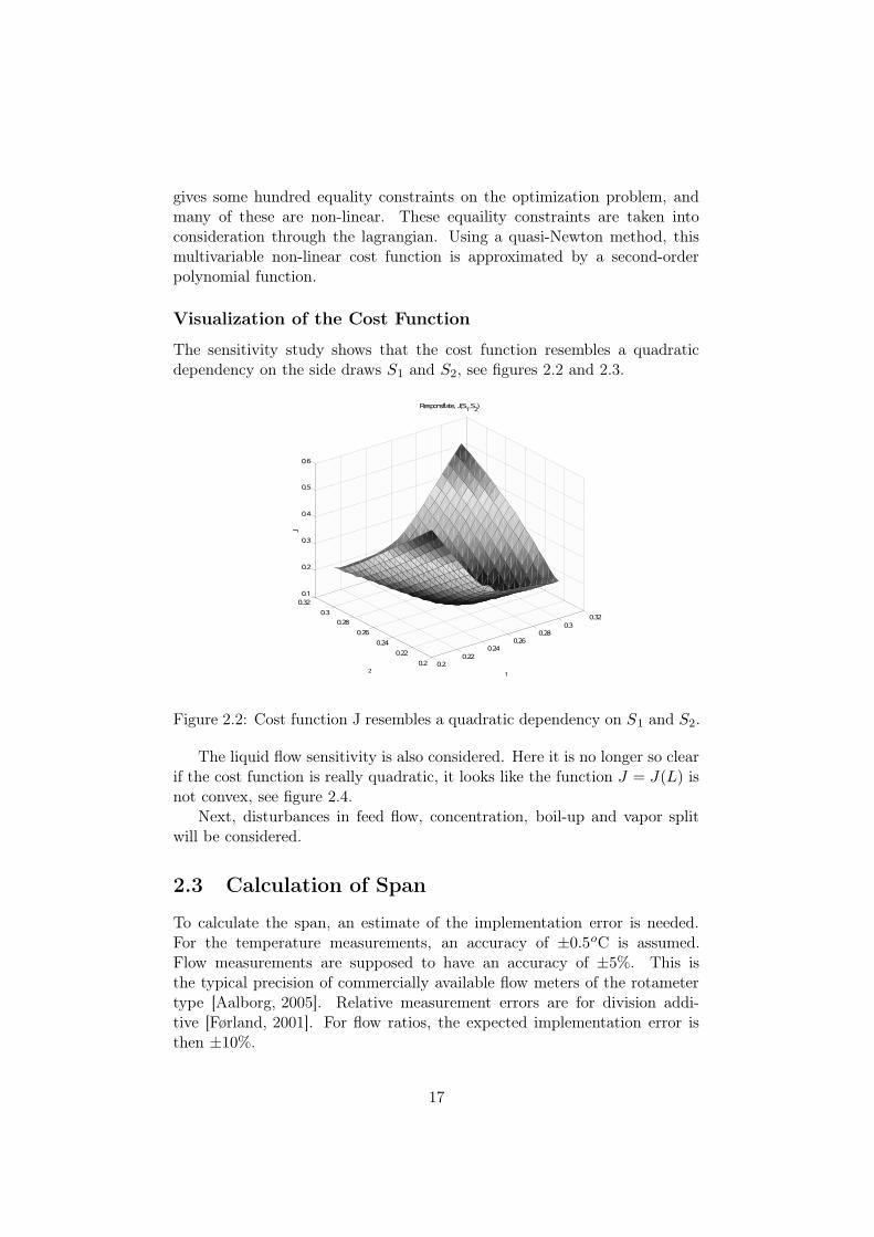
Visualization of the Cost Function

The sensitivity study shows that the cost function resembles a quadraticdependency on the side draws S1 and S2, see figures 2.2 and 2.3.

Figure 2.2: Cost function J resembles a quadratic dependency on S1 and S2.

The liquid flow sensitivity is also considered. Here it is no longer so clearif the cost function is really quadratic, it looks like the function J = J(L) isnot convex, see figure 2.4.

Next, disturbances in feed flow, concentration, boil-up and vapor splitwill be considered.

2.3 Calculation of Span

To calculate the span, an estimate of the implementation error is needed.For the temperature measurements, an accuracy of ±0.5oC is assumed.Flow measurements are supposed to have an accuracy of ±5%. This isthe typical precision of commercially available flow meters of the rotametertype [Aalborg, 2005]. Relative measurement errors are for division addi-tive [Førland, 2001]. For flow ratios, the expected implementation error isthen ±10%.

17

Figure 2.3: Cost function J resembles a quadratic dependency on S1 and S2.

To caculate the span, an estimate of the optimization error is needed.This is calculated as the optimal variation:

∆eopt =max zi − min zi

2(2.2)

2.3.1 Problems in the calculation

The effect of the disturbances on J were of similar magnitude, except forthe boil-up, which had a much stronger effect on the cost function. A per-turbation of 1% in the other disturbances F, ziF , RV gave changes in theobjective function of 1 to 12 %, whereas a perturbation in the boil-up gavea change of 70%. An optimization gave solution at J = 0.1631. This is stillquite far from 0.1299, so a bracketing calculation was performed to enclosethe optimum. However, bracketing with 4 degrees of freedom is a tedioustask, and at last the solution was kept at J = 0.1365. For full description ofthe bracketing procedure, see appendix A.

2.4 The Scaled Gain Matrix and Optimal Selection

The model was slightly perturbed in the inputs to find the steady-state gain.The gain matrix was then scaled by the span for each variable (each row isdivided by the span of the variable). The scaled gain calculation was doneusing Excel. This scaled gain matrix was then exported to MATLAB, usingthe built-in Excel link.

18

3.04 3.045 3.05 3.055 3.06 3.065 3.07 3.0750.125

0.13

0.135

0.14

0.145

0.15

0.155

0.16

0.165

0.17

L [kmol/h]

J

Figure 2.4: The cost function shows a non-quadratic dependence on liquidflow.

A branch and bound algorithm by Cao [Cao and Rossiter, 1997] was usedto find the 3 best solutions (the 3 combinations that yield the maximumminimum singular value). This was done once with all considered variables,and once with only temperature measurements allowed. The results wereas shown in Tables 2.3 and 2.4. The difference in singular values is notthat big, so it might be that a selection of just temperature measurementsin practice is just as good as one including internal flow ratios.

Rank z1 z2 z3 z4 Singular Value

1 T5 − TS4 V/B T3 − TS2 T8 − TS1 407.92 T5 − TS4 L/D T3 − TS2 T8 − TS1 407.83 T5 − TS4 V/B T3 − TS2 T7 − TS1 407.7

Table 2.3: Best selections - full variable set. TS refers to figure 2.1 onpage 15.

Rank z1 z2 z3 z4 Singular Value

1 T5 − TS4 TReboiler T5 − TS2 T6 − TS1 312.82 T5 − TS4 TReboiler T5 − TS2 T5 − TS1 312.53 T5 − TS4 T8 − TS2 T5 − TS2 T6 − TS1 311.7

Table 2.4: Best selections - temperatures.Also here, TS refers to figure 2.1on page 15.

19

2.4.1 Loss Calculations

Loss calculations are performed to see if the preliminary results are promis-ing. Some indicated measurement combinations may be infeasible, whichcan only be detected through a brute force calculation.

Full Set of Candidate Variables

A loss calculation was performed using the Hysys model. Rank 1 in 2.3was infeasible, rank 2 was feasible but gave a negative loss for the vaporflow (boil-up, V ) disturbance (L = -0.006). This shows that the bracketingoperation had not located the real optimum. This problem may have severalreasons:

• Non-convex optimization problem

• Numerical Precision problems in Hysys

It seems that the first possible reason is the one causing problems (dueto non-convexity). This affects the scaling of the gain matrix, because thecalculated scaling is based on an erroneous estimate of the optimal variation.However, the selection of the optimal set is probably not too sensitive to thescaling. In order to find a better estimate of the optimal variation, and abetter scaling, a method for correcting the start condition of the gradientbased optimization in Hysys is suggested, see section 2.5.

This method was used to recalculate the scaling for the gain matrix, andthe selection was calculated again using the branch and bound method ofCao. The results are given in Table 2.5

Rank z1 z2 z3 z4 Singular Value

1 T5 − TS4 L/D T3 − TS2 T8 − TS1 406.92 T5 − TS4 L/D T8 − TS3 T9 − TS1 406.83 T5 − TS4 V/B T3 − TS2 T7 − TS1 406.6

Table 2.5: Best selections after scaling update - full variable set. TS refersto figure 2.1 on page 15.

The loss calculation yields that the combination with rank 3 is infeasible,and the two first combinations are both very good candidates, see Table 2.6

SVD Rank Loss

1 0.00052 0.00053 INFEASIBLE

Table 2.6: Loss calculation - full variable set

20

Temperature Subset Selection

After the discrepancy in the reoptimization at the boil-up disturbance, thetemperature selection was also recalculated, but the optimal selection did notchange. Hence, the selection shown in Table 2.4 is used in the calculations.However, the singular values changed slightly. The new singular values are:

• Rank 1: 312.5

• Rank 2: 312.2

• Rank 3: 311.5

These are still very similar. That is, the losses should not differ very much.However, what happens, is that no solution is found when the temperaturesgiven in Table 2.4 are used as specifications in Hysys. This is because, thesecannot be kept at constant values when other process variables are changed.The situation is probably caused because there are two temperature specifi-cations in section TS2, which causes the system to be overdetermined 1.

It seems that the loss is not very dependent on the choice of the con-trolled variables, as long as the selection is feasible. This is a very attractivesituation. Based on intuition, the following temperatures were selected:

• T5 − TS1: To stabilize the temperature profile in the prefractionator.

• T7 − TS2: Close to the reboiler, to control the purity of the bottomproduct.

• T4 − TS3: Lower part of main tower: Temperature profile control.

• T4 − TS5: Upper part of main tower: Temperature profile control

A brute force calculation with these temperatures kept at their nominalvalues, shows that the loss is practically zero. It seems that the importantquestion in this case is ”at what setpoints should we control the plant”, andnot ”what should be controlled”.

2.5 Startvalue Correction for Optimization

As explained in section 2.4.1, problems with non-convexity are often encoun-tered. An outline of an algorithm to overcome this, is given in figure 2.5.

The fix is simply to use the best feasible solution indicated by the sin-gular value method, using the initial scaling. Then the indicated variablesare used as specifications in Hysys, and a new starting point for the reop-timization is calculated. Then the process is optimized again, and this is

1Where Hysys gives the somewhat cryptical error message: "Singular Column Matrix:

Possibly no physical solution at given conditions"

21

Figure 2.5: A method to overcome convexity problems

done iteratively untill the loss (L) is positive. Mostly, only one iteration isrequired. An illustration of what the start value correction does, is given infigure 2.6. A disturbance moves the state as shown, and a gradient basedoptimization method wil then converge to a local minimum. A correctionusing the solution indicated by the singular value analysis, moves the stateto a point closer to the global minimum, and the optimization then has apossibility of converging to the best solution.

22

0 2 4 6 8 10 120

0.1

0.2

0.3

0.4

0.5

0.6

0.7

0.8

d

J

Start

STEP IN d

Local Optimum

SVDSuggestedSolution

Figure 2.6: Effect of correcting the start values

23

Chapter 3

Control Configuration

An analysis of which variables to be controlled has been done. The analysisindicated that the selection of controlled variables is not critical for thisapplication.

3.1 Control with Four Temperature Measurements

For the following analysis, the four temperatures indicated on page 21 arechosen as controlled variables, as shown in figure 3.1.

Figure 3.1: Temperature measurements in the control analysis

24

A dynamic simulation in Hysys was attempted to assist controller designand tuning, but the model was to unstable to be of any use. A step in anyof the inputs gave large oscillations or convergence toward some solutionoutside the physical variable domain (negative pressures and mole fractions,for instance).

The pairing is done with regard to short loops. The prefractionatormeasurement T5 − TS1 is then to be controlled using the liquid split (RL).T4 −TS5 is controlled with the liquid flow (reflux, L), T4 −TS3 with S1 andT7−TS2 with S2. The control could probably be done using PID controllers,because the measurements are not too close, such that heavy interactions arenot expected. However, to determine this, dynamic simulations are neces-sary.

3.2 Sensitivity Analysis

In order to analyse the potential of the chosen outputs as good controlledvariables, a sensitivity study was performed.

In the prefractionator, y1 = T5 − TS1 was chosen as controlled variable.Keeping all other controlled variables constant, the column purity (the costfunction, J) showed to be not very dependent on the value of y1, which isan attractive situation. The result is given in fig 3.2 on page 27.

The top measurement in the main tower showed a much narrower min-imum. This is not so attractive, and here the position of the measurementmay be more important. The sensitivity analysis result is given in 3.3.

The lower measurement in the main tower is problematic. The sensitivityanalysis gives a picture of the non-convexity of the optimization problem usedin the first part of this work, see figure 3.4. The minimum is very narrow,hence y3 = T4 − TS3 is a bad choice for a controlled variable.

Regarding y, see 3.5, the minimum is even narrower. The allowable rangeof y4 narrower than the precision in a temperature measurement, hence theuse of this variable will probably lead to controllability problems.

It seems that it is not a good idea, to try to control the lower temperaturesin the column. The prefractionator temperature is ok.

The singular value method indicated that 3 temperatures and a flow ratioshould be controlled. This might be a better solution.

25

3.3 Results from the Singular Value Rule

The singular value rule gave the following suggestion for the controlled vari-ables:

• z1 = T5 − TS4

• z2 = V/B

• z3 = T3 − TS2

• z4 = T8 − TS1

These outputs may be better to use for control, than using just temperatures,because one avoids measurements very close to the reboiler. That is, oneavoids temperature measurement, where the allowable variation is smallerthan the measurement accuracy. The pairing would be done such that shortloops are achieved. Some interaction between the controlled variables isto be expected. To see if self-optimizing control can be achieved, dynamicsimulations must be done. If self-optimizing control can not be achieved, itmight be worth considering multivariable control from the layer above, usingthe set-points in the regulatory layer as degrees of freedom.

26

Figure 3.2: Purity, J , as a function of prefractionator temperature specifica-toin, y1 = T5 − TS1

Figure 3.3: Purity, J , as a function of temperature specification, y2 = T4 −TS5

27

Figure 3.4: Purity, J , as a function of temperature specification, y3 = T4 −TS3. A very narrow minimum.

Figure 3.5: Purity, J , as a function of temperature specification, y4 = T7 −TS2. A very narrow minimum.

28

Chapter 4

Concluding Remarks

In this report, it is shown that Hysys can be used for steady-state analysisof custom processes. It is, however, also found that Hysys is not good fordynamic simulation, at least, the model used for steady-state analysis cannot be used.

The singular value rule is applied to the Kaibel column control structureproblem, and from a steady-state point of view a good solution has beenfound. The indicated best solution, surprisingly, includes other measure-ments than just stage temperatures.

Some measures to handle non-convexity and problems with convergenceare also introduced, using the singular value rule to correct the star valuesfor optimization, using a reduced gradient method in the optimizer. Thesuccess of this method, requires that the steady-state gain of the processmodel is obtained close to the optimum also of the disturbed process. Thisrequires that the global optimum does not move very much when the processis disturbed.

29

Appendix A

Bracketing Calculations

For the calculation of the optimal inputs when a disturbance in the boil-upoccurs, a bracketing procedure was used. This is simply varying the inputs tolocate where the optimum might be. For a non-convex multivariable problemthis is a very tedious task, and hence it is mostly used in 1-dimensional opti-mization, as pre-optimization for gradient based methods. The calculationsfor the boil-up are summarized in Table A.1.

Test No. S1 S2 L RL J

1 0.22 0.22 NC NC 0.33402 0.24 0.24 NC NC 0.17943 0.26 0.26 NC NC 0.3157.. ... ... ... ... ...

.. 0.2442 0.2490 3.07 0.2699 0.1365

Table A.1: Bracketing Calculations

The bracketing is meant to close in the optimum, so that the optimizercan be given limits on the search region.

30

Appendix B

Software Descriptions

In the calculations, software from different vendors has been used. A shortdescription of each program will be given, and a description of connectingcalculations will follow.

Excel

Microsoft Excel 2003 is used to calculate the gain matrix, the span and forvisualizing sensitivity calculations.

Hysys

Hysys v3.2. is a process flowsheet simulator, which is used to simulate theKaibel distillation process at steady-state. The program includes an opti-mization tool, which is used to perform local optimization.

MATLAB

MATLAB version 7.1 from MathWorks was used for branch and bound se-lection calculations and plotting of sensitivity graphics.

Automation and Software Connectivity

The sensitivity studies were automated using macros written in Visual Basicfor Applications (VBA) in Excel. The Hysys object library is available toVisual Basic through an extensive application programming interface (API)and can be imported into the VBA object library.

Data exchange between MATLAB and Excel is also easy to implement,thanks to the Excel link package in MATLAB 7.1. Data can be read fromand written to Excel Worksheets using simple MATLAB functions.

31

Bibliography

[Aalborg, 2005] Aalborg (2005). Website of flow sensor vendor:http//www.aalborg.com.

[Cao and Rossiter, 1997] Cao, Y. and Rossiter, D. (1997). An input pre-screening technique for control structure selection. Computers chem. En-gng., 21:563–569.

[Elliot and Lira, 1999] Elliot, J. R. and Lira, C. T. (1999). IntroductoryChemical Engineering Thermodynamics. Prentice-Hall.

[Førland, 2001] Førland, K. S. (2001). Kvantitativ Analyse. Tapir AkademiskForlag, Trondheim, 2 edition.

[Kaibel et al., 2004] Kaibel, G., Miller, C., Stroezel, M., von Watzdorf, R.,and Jansen, H. (2004). Industrieller einsatz von trennwandkolonnen undthermisch gekoppelten destillationskolonnen. Chemie Ingenieur Technik,76:258 – 263.

[Nocedal and Wright, 1999] Nocedal, J. and Wright, S. J. (1999). NumericalOptimization. Springer Verlag, New York.

[Skogestad, 1997] Skogestad, S. (1997). Dynamics and control of distillationcolumns - a tutorial introduction. Trans. IChemE, Part A, 75.

[Skogestad and Postlethwaite, 2005] Skogestad, S. and Postlethwaite, I.(2005). Multivariable Feedback Control - Analysis and Design. John Wiley& Sons, Ltd., Chichester, 2nd. edition.

[Strandberg and Skogestad, 2005] Strandberg, J. and Skogestad, S. (2005).Stabilizing control of an integrated 4-product kaibel column.

[Wenzel and Röhm, 2003] Wenzel, S. and Röhm, H.-J. (2003). Ausle-gung thermisch und stofflich gekoppelter destillationskolonnen mittelsgesamtkostenoptimierung. Chemie Ingenieur Technik, 75:534–540.

32