
Self-assembling fractal particle networks
75
Self-assembling fractal particle networks Joseph Jun and Alfred Hübler Center for Complex Systems Research University of Illinois at Urbana- Champaign Research supported in part by the National Science Foundation (PHY-01-40179 and DMS-03725939 ITR)
-
Upload
kathleen-weaver -
Category
Documents
-
view
23 -
download
1
description
Self-assembling fractal particle networks. Joseph Jun and Alfred Hübler Center for Complex Systems Research University of Illinois at Urbana-Champaign. Research supported in part by the National Science Foundation ( PHY-01-40179 and DMS-03725939 ITR ). - PowerPoint PPT Presentation
Transcript of Self-assembling fractal particle networks
Self-assembling fractal particle networks
Joseph Jun and Alfred Hübler
Center for Complex Systems ResearchUniversity of Illinois at Urbana-
ChampaignResearch supported in part by the National Science
Foundation
(PHY-01-40179 and DMS-03725939 ITR)
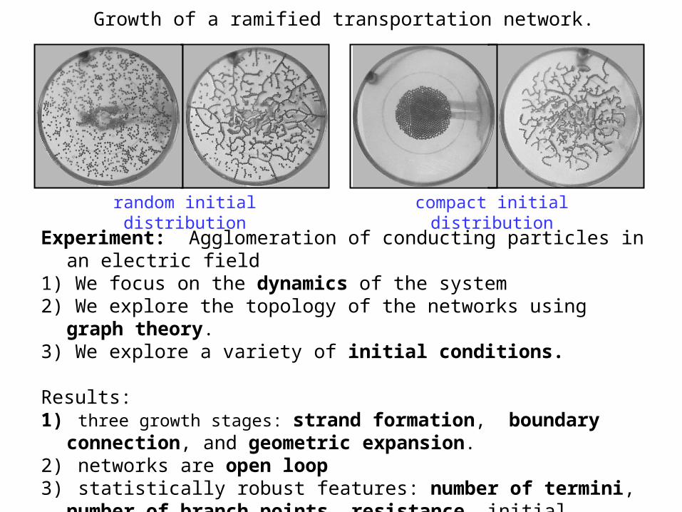
Growth of a ramified transportation network.
Experiment: Agglomeration of conducting particles in an electric field1) We focus on the dynamics of the system2) We explore the topology of the networks using graph theory.3) We explore a variety of initial conditions.
Results:1) three growth stages: strand formation, boundary connection, and
geometric expansion. 2) networks are open loop 3) statistically robust features: number of termini, number of branch points,
resistance, initial condition matters somewhat4) Minimum spanning tree growth model predicts emerging pattern
random initial distribution compact initial distribution
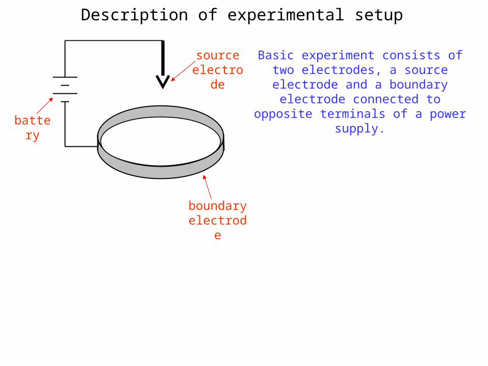
Description of experimental setup
Basic experiment consists of two electrodes, a source electrode and a boundary electrode connected to opposite terminals of a power
supply.
source electrod
e
boundary electrode
battery
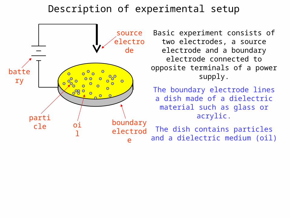
Description of experimental setup
Basic experiment consists of two electrodes, a source electrode and a boundary electrode connected to opposite terminals of a power
supply.
The boundary electrode lines a dish made of a dielectric material
such as glass or acrylic.
The dish contains particles and a dielectric medium (oil)
source electrod
e
boundary electrode
oil
battery
particle
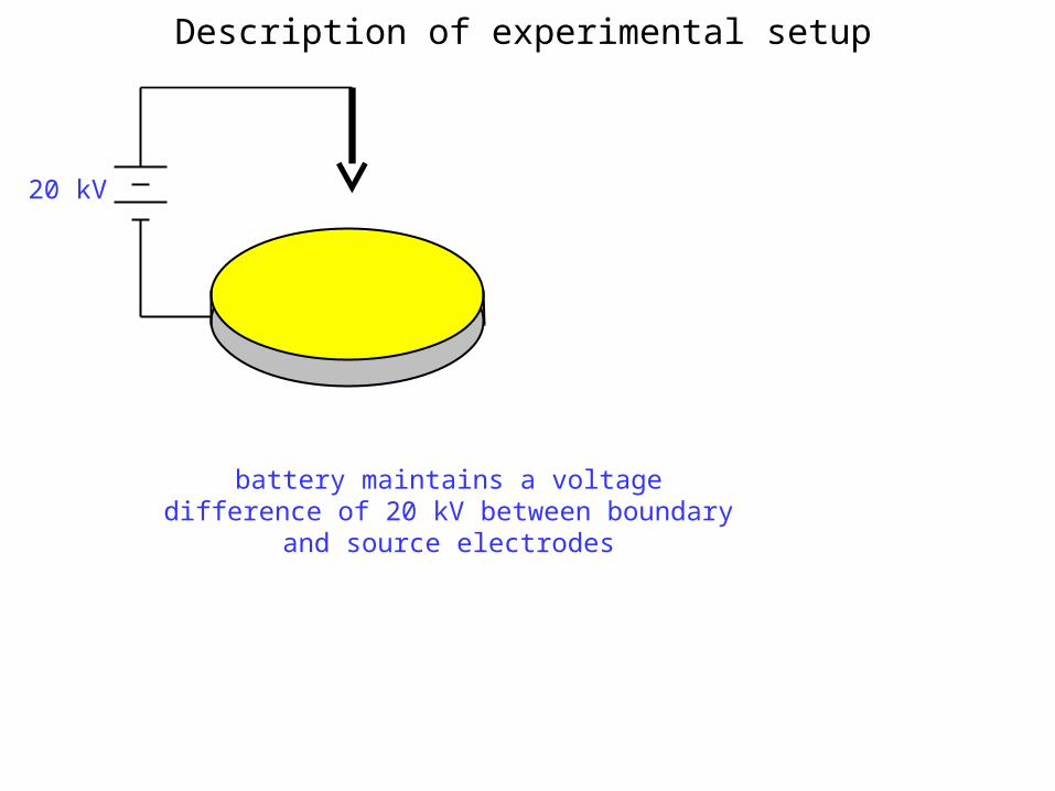
Description of experimental setup
20 kV
battery maintains a voltage difference of 20 kV between boundary and source
electrodes
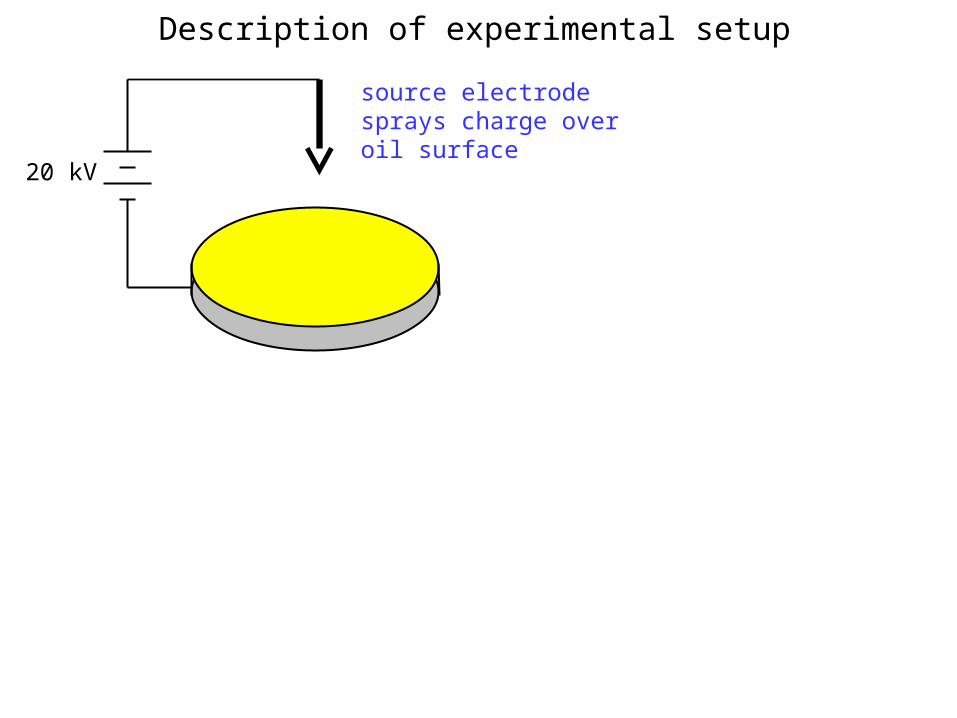
Description of experimental setup
20 kV
source electrode sprays charge over oil surface
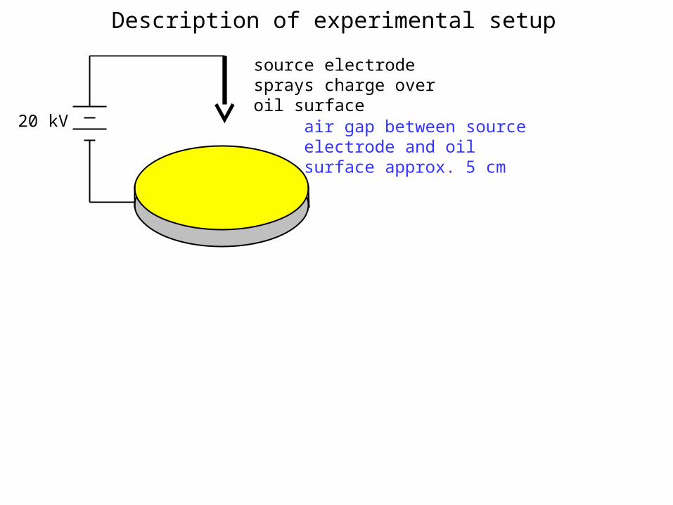
Description of experimental setup
20 kV
source electrode sprays charge over oil surface
air gap between source electrode and oil surface approx. 5 cm
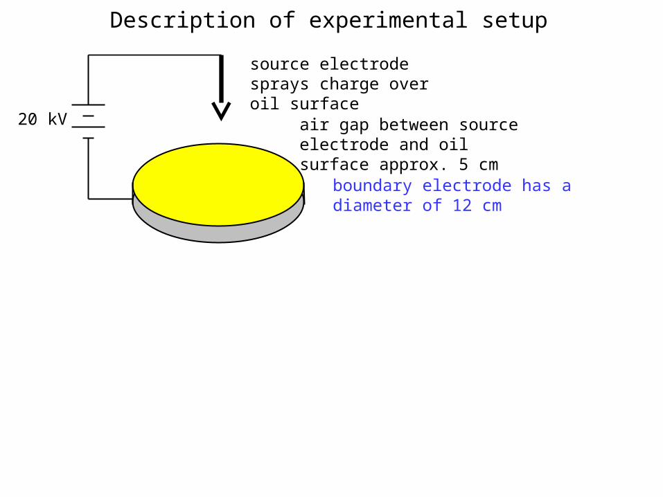
Description of experimental setup
20 kV
source electrode sprays charge over oil surface
air gap between source electrode and oil surface approx. 5 cm
boundary electrode has a diameter of 12 cm
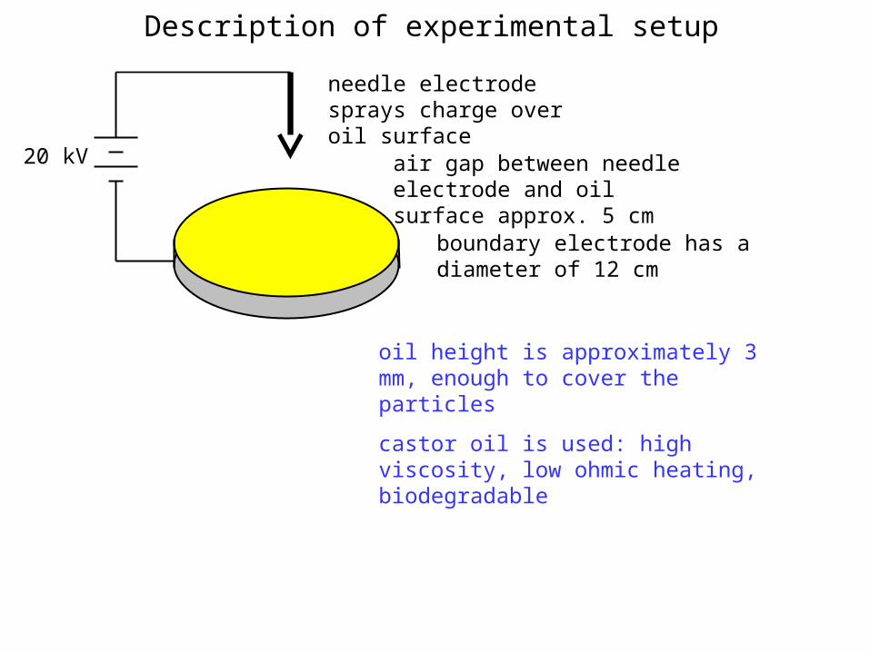
Description of experimental setup
20 kV
needle electrode sprays charge over oil surface
air gap between needle electrode and oil surface approx. 5 cm
boundary electrode has a diameter of 12 cm
oil height is approximately 3 mm, enough to cover the particles
castor oil is used: high viscosity, low ohmic heating, biodegradable
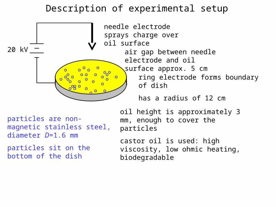
Description of experimental setup
20 kV
needle electrode sprays charge over oil surface
air gap between needle electrode and oil surface approx. 5 cm
ring electrode forms boundary of dish
has a radius of 12 cm
oil height is approximately 3 mm, enough to cover the particles
castor oil is used: high viscosity, low ohmic heating, biodegradable
particles are non-magnetic stainless steel, diameter D=1.6 mm
particles sit on the bottom of the dish
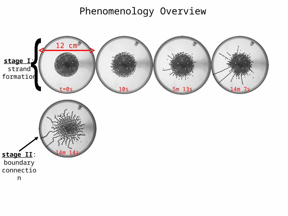
Phenomenology
The growth of the network proceeds in three stages: I) strand formation
II) boundary connection
III) geometric expansion
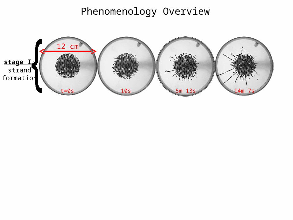
Phenomenology Overview
12 cm
t=0s 10s 5m 13s 14m 7s
stage I:strand
formation
Phenomenology Overview
12 cm
t=0s 10s 5m 13s 14m 7s
14m 14s
stage I:strand
formation
stage II:boundary
connection
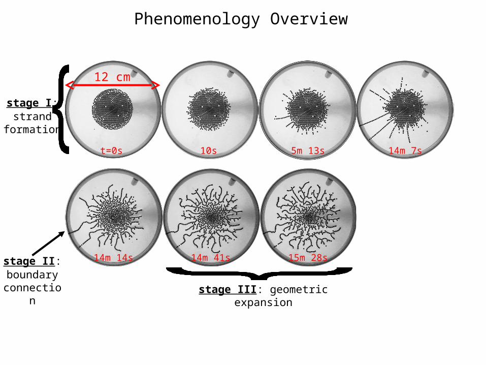
Phenomenology Overview
12 cm
t=0s 10s 5m 13s 14m 7s
14m 14s 14m 41s 15m 28s
stage I:strand
formation
stage II:boundary
connection stage III: geometric expansion
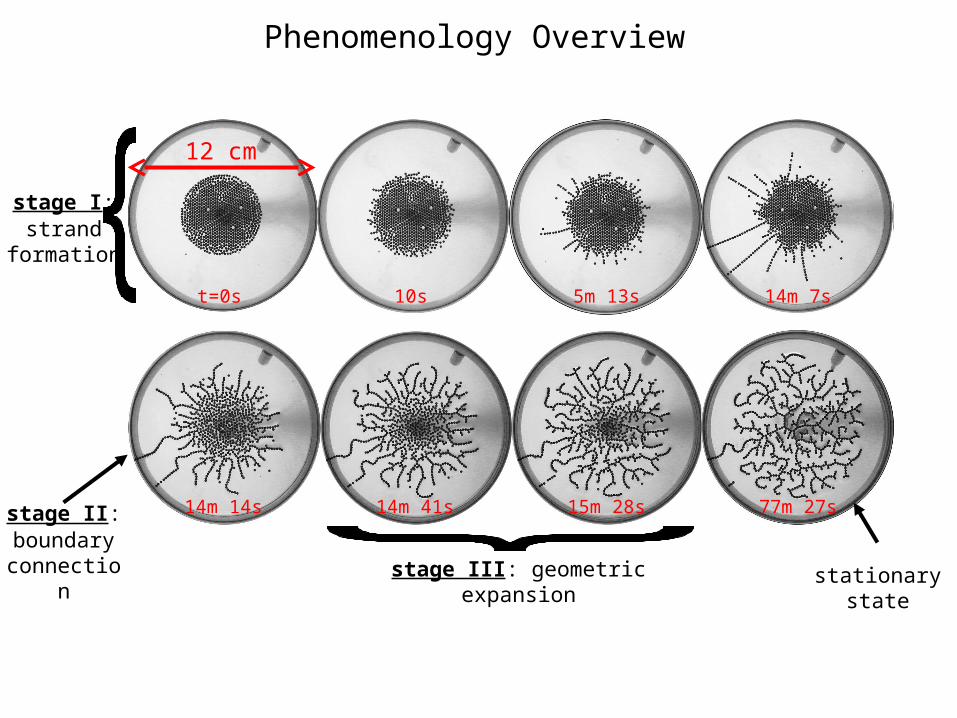
Phenomenology Overview
12 cm
t=0s 10s 5m 13s 14m 7s
14m 14s 14m 41s 15m 28s 77m 27s
stage I:strand
formation
stage II:boundary
connection stage III: geometric expansion
stationary state
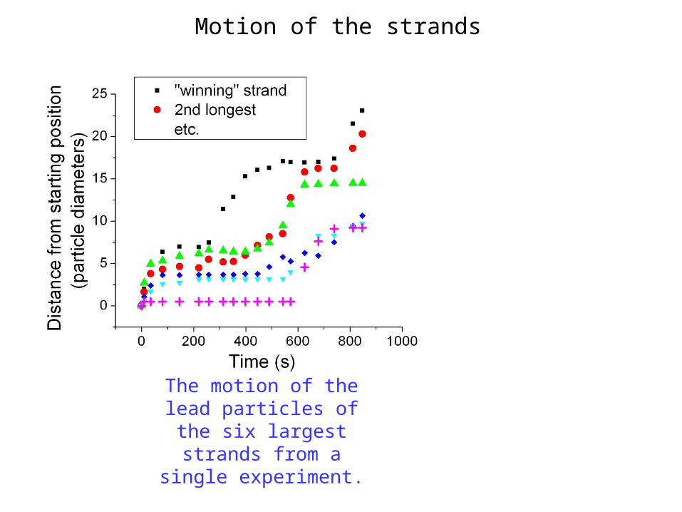
Motion of the strands
The motion of the lead particles of the six
largest strands from a single experiment.
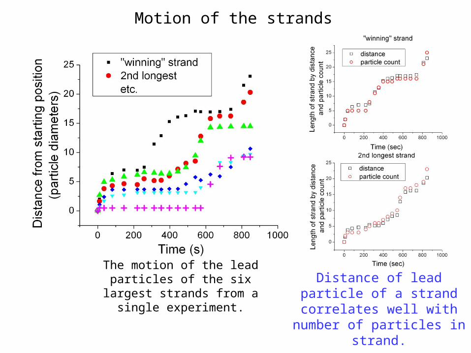
Motion of the strands
The motion of the lead particles of the six largest
strands from a single experiment.
Distance of lead particle of a strand correlates well with number of particles
in strand.
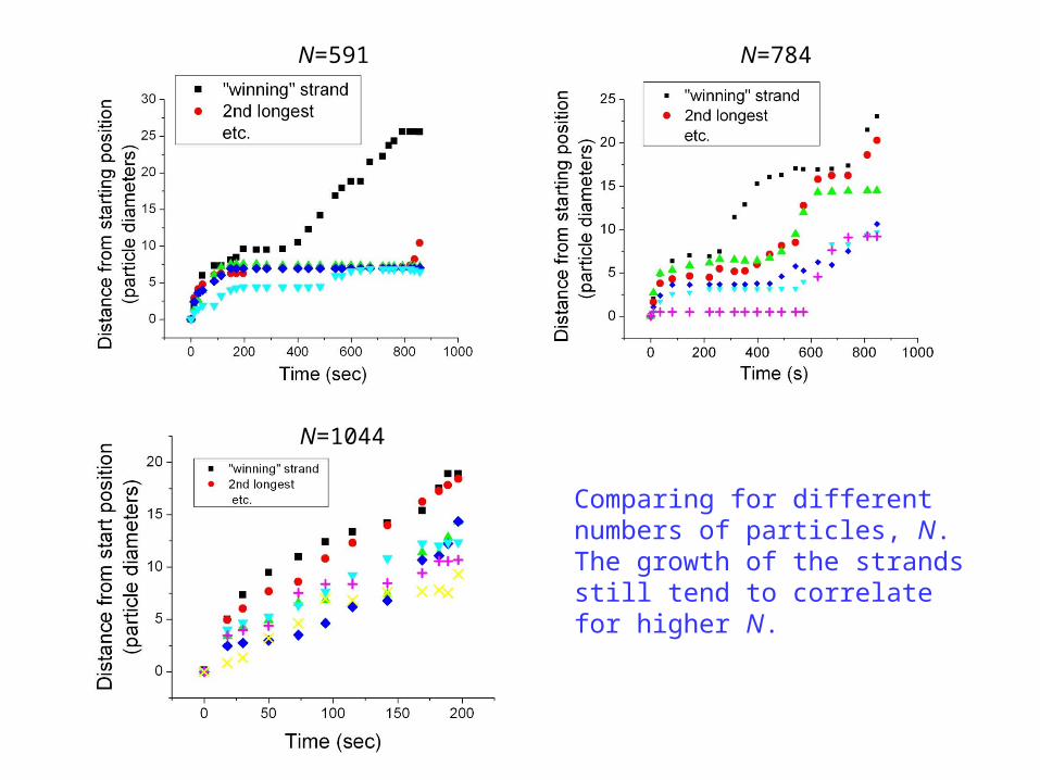
N=1044
N=591 N=784
Comparing for different numbers of particles, N. The growth of the strands still tend to correlate for higher N.

Phenomenology: stage II (boundary connection)
Stage II begins when the “winning” strand connects to the boundary. It is brief in duration, and is best characterized by the particles binding to the boundary.
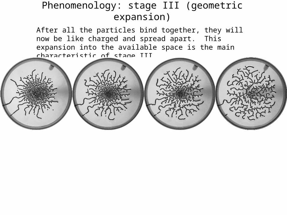
Phenomenology: stage III (geometric expansion)
After all the particles bind together, they will now be like charged and spread apart. This expansion into the available space is the main characteristic of stage III.
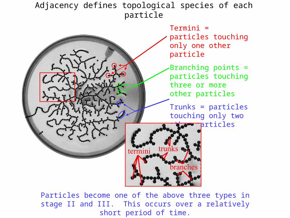
Adjacency defines topological species of each particle
Termini = particles touching only one other particle
Branching points = particles touching three or more other particles
Trunks = particles touching only two other particles
Particles become one of the above three types in stage II and III. This occurs over a relatively short period of time.
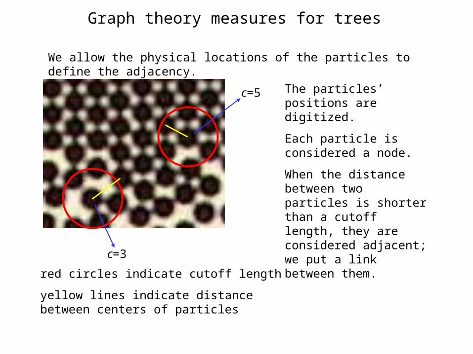
Graph theory measures for trees
We allow the physical locations of the particles to define the adjacency.
c=5
c=3
The particles’ positions are digitized.
Each particle is considered a node.
When the distance between two particles is shorter than a cutoff length, they are considered adjacent; we put a link between them.
red circles indicate cutoff length
yellow lines indicate distance between centers of particles
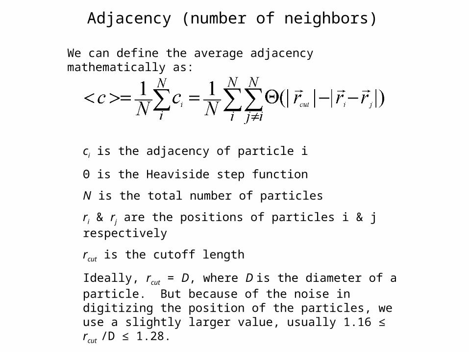
Adjacency (number of neighbors)
We can define the average adjacency mathematically as:
ci is the adjacency of particle i
Θ is the Heaviside step function
N is the total number of particles
ri & rj are the positions of particles i & j respectively
rcut is the cutoff length
Ideally, rcut = D, where D is the diameter of a particle. But because of the noise in digitizing the position of the particles, we use a slightly larger value, usually 1.16 ≤ rcut /D ≤ 1.28.
Also ideally, 0 ≤ ci ≤ 6; we impose this by hand in the algorithm.
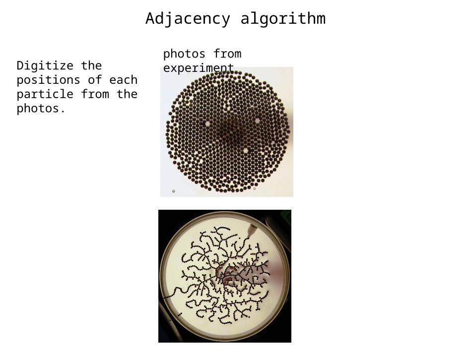
Adjacency algorithm
Digitize the positions of each particle from the photos.
photos from experiment
Adjacency algorithm
Digitize the positions of each particle from the photos.
Run the adjacency algorithm on the list of particle positions.
photos from experiment
digitization of positions

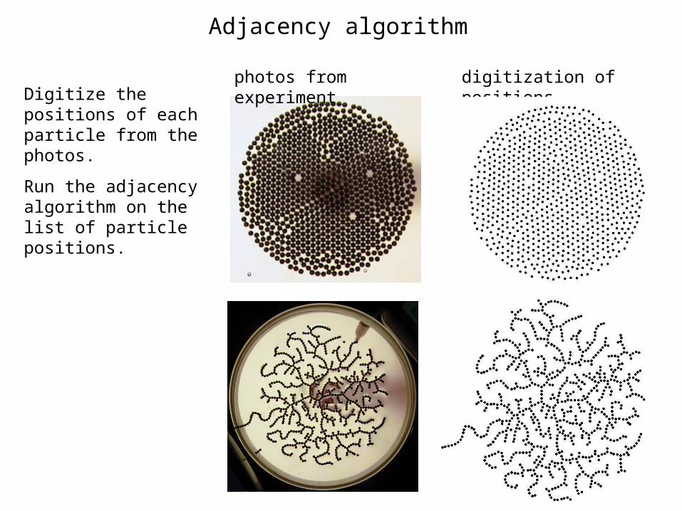
Adjacency algorithm
Digitize the positions of each particle from the photos.
Run the adjacency algorithm on the list of particle positions.
The algorithm picks up how particles are connected. It identifies holes and grain boundaries.
*Graphs from algorithm were visualized using the Combinatorica package in Mathematica.rcut =
1.25•D
photos from experiment
output from algorithm*
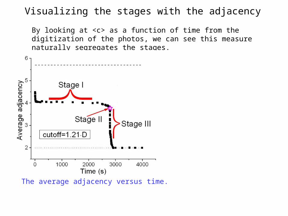
Visualizing the stages with the adjacency
By looking at <c> as a function of time from the digitization of the photos, we can see this measure naturally segregates the stages.
The average adjacency versus time.
Visualizing the stages with the adjacency
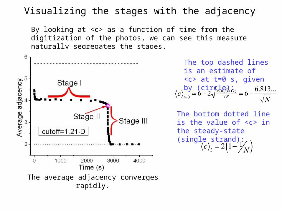
By looking at <c> as a function of time from the digitization of the photos, we can see this measure naturally segregates the stages.
The top dashed lines is an estimate of <c> at t=0 s, given by (circle):
The bottom dotted line is the value of <c> in the steady-state (single strand):
The average adjacency converges rapidly.
Visualizing the stages with the adjacency
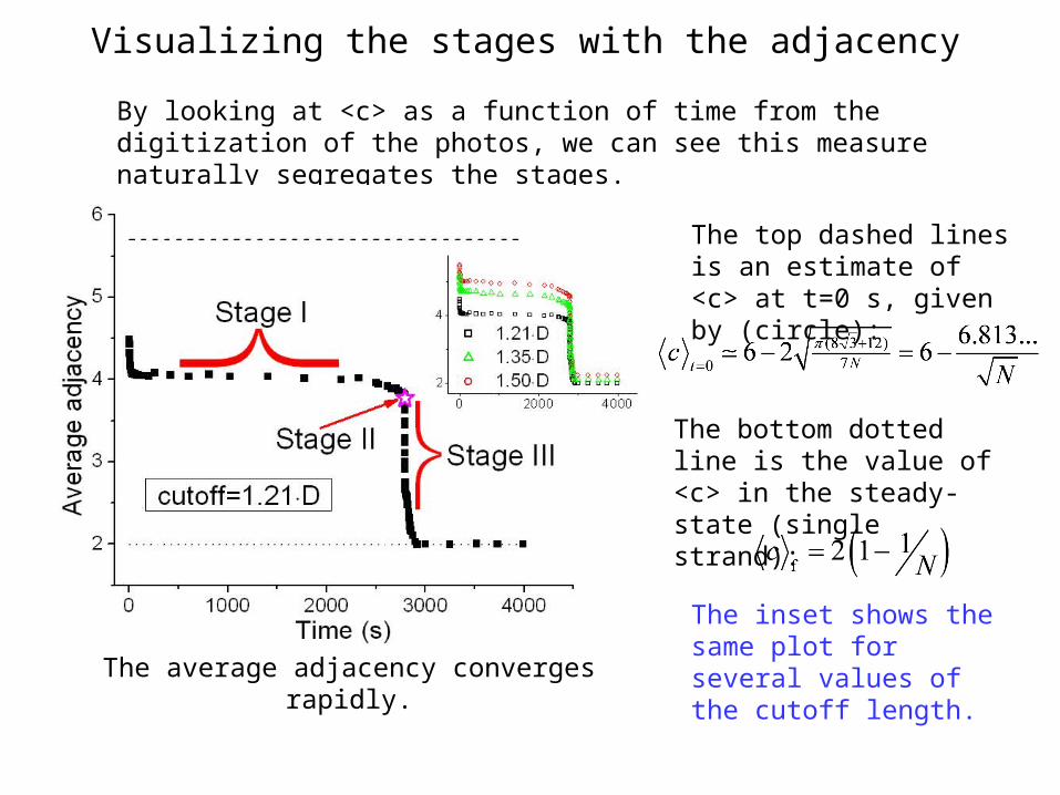
By looking at <c> as a function of time from the digitization of the photos, we can see this measure naturally segregates the stages.
The top dashed lines is an estimate of <c> at t=0 s, given by (circle):
The bottom dotted line is the value of <c> in the steady-state (single strand):
The inset shows the same plot for several values of the cutoff length.
The average adjacency converges rapidly.
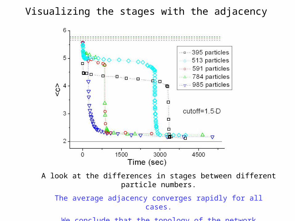
Visualizing the stages with the adjacency
A look at the differences in stages between different particle numbers.
The average adjacency converges rapidly for all cases.
We conclude that the topology of the network establishes in a relatively short amount of time following stage II.
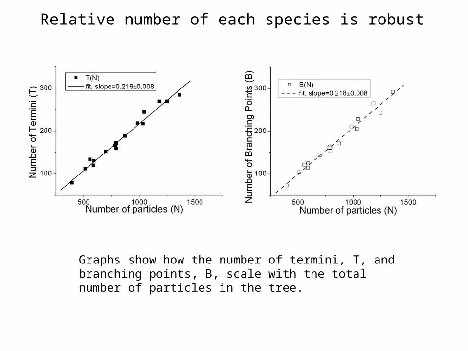
Relative number of each species is robust
Graphs show how the number of termini, T, and branching points, B, scale with the total number of particles in the tree.
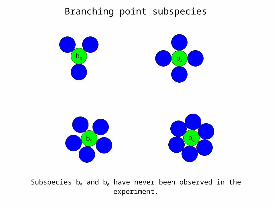
Branching point subspecies
Subspecies b5 and b6 have never been observed in the experiment.
b3 b4
b5 b6
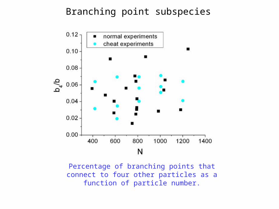
Branching point subspecies
Percentage of branching points that connect to four other particles as a function of
particle number.
Most networks are trees.Only a few rare cases contain loops
(cycles).

Loops (cycles) are unstable
Insets on the left show two particles artificially placed into a loop separate from one another.
The graph on the right shows the separation between the two particles as a function of time.
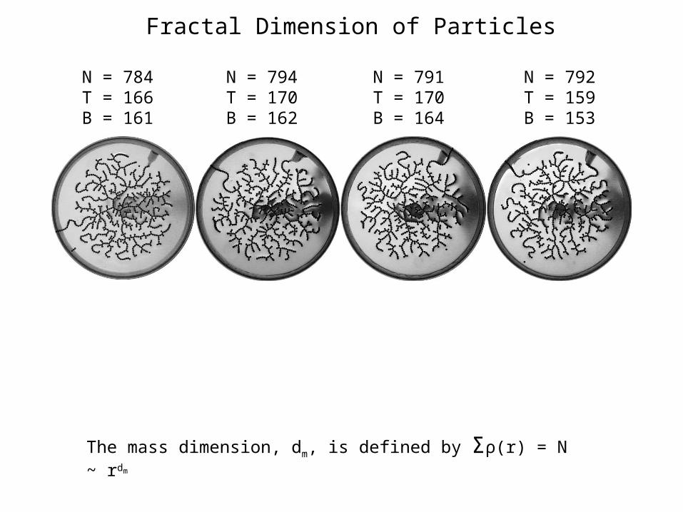
Fractal Dimension of Particles
N = 792T = 159B = 153
N = 791T = 170B = 164
N = 794T = 170B = 162
N = 784T = 166B = 161
The mass dimension, dm, is defined by Σρ(r) = N ~ rdm
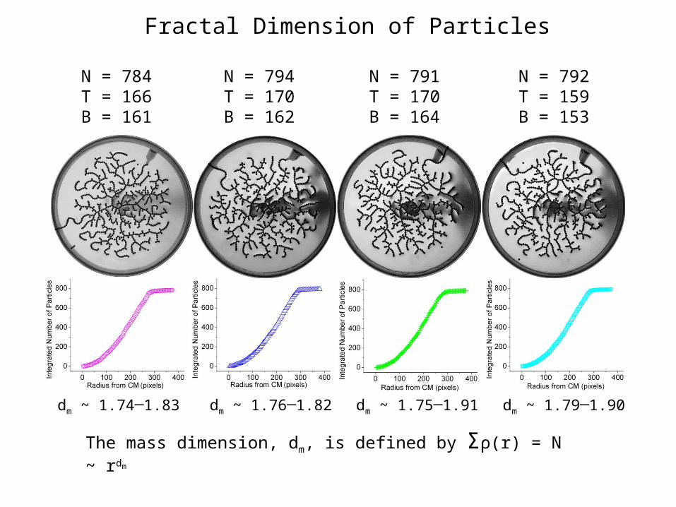
Fractal Dimension of Particles
N = 792T = 159B = 153
N = 791T = 170B = 164
N = 794T = 170B = 162
N = 784T = 166B = 161
dm ~ 1.74─1.83 dm ~ 1.76─1.82 dm ~ 1.75─1.91 dm ~ 1.79─1.90
The mass dimension, dm, is defined by Σρ(r) = N ~ rdm
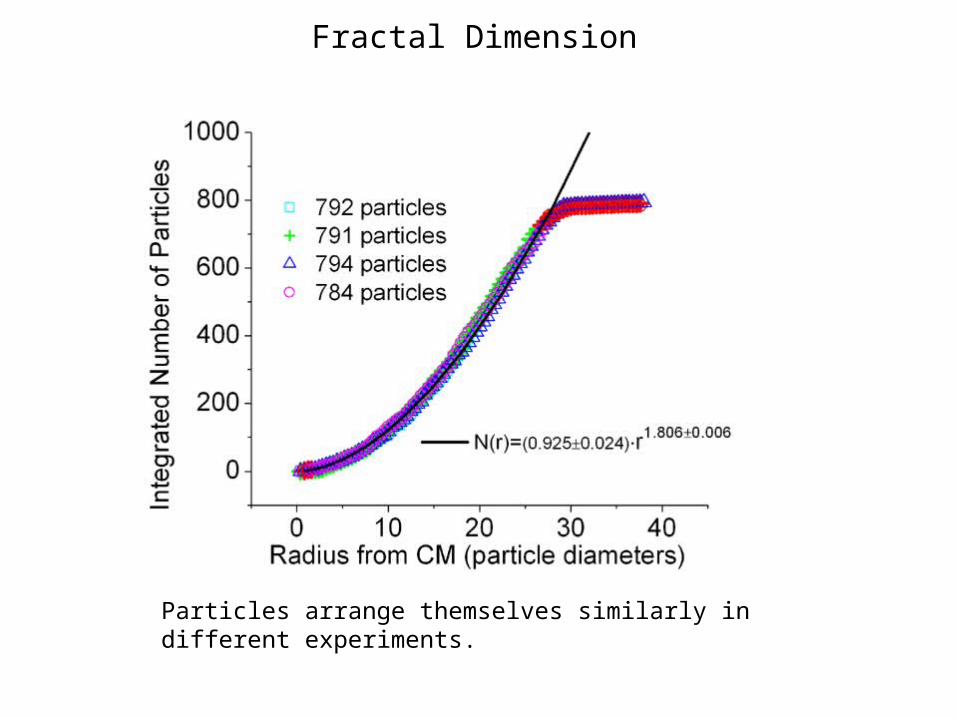
Fractal Dimension
Particles arrange themselves similarly in different experiments.
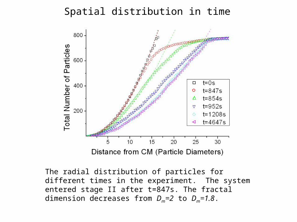
Spatial distribution in time
The radial distribution of particles for different times in the experiment. The system entered stage II after t=847s. The fractal dimension decreases from Dm=2 to Dm=1.8.
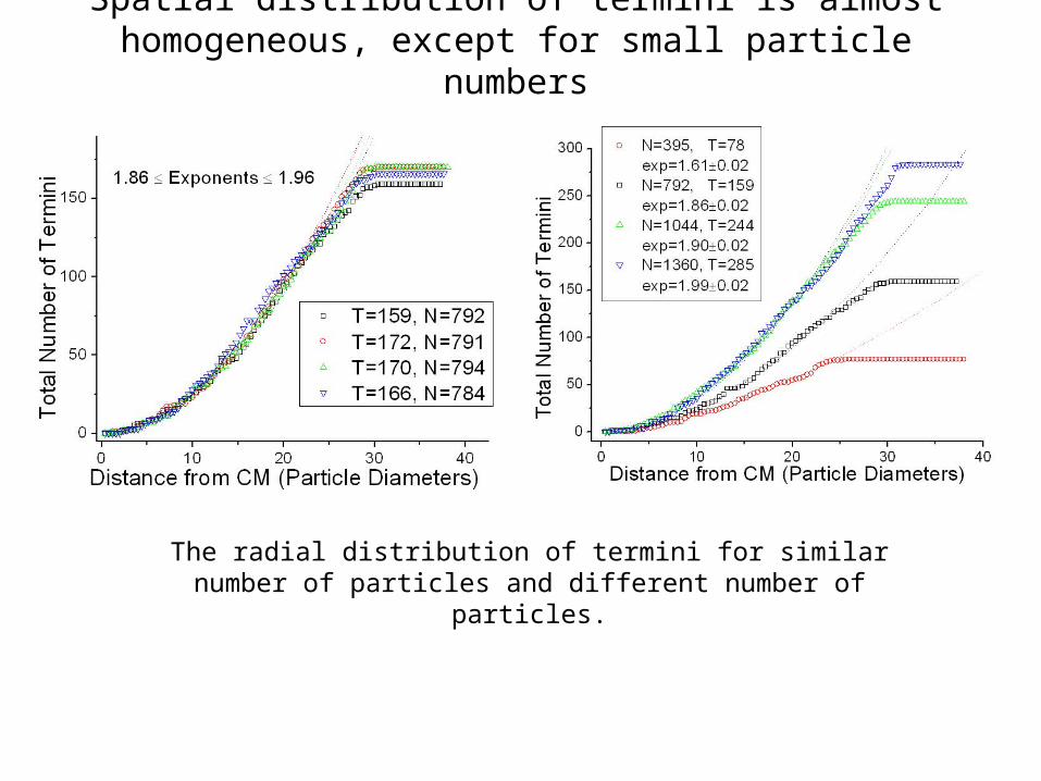
Spatial distribution of termini is almost homogeneous, except for small particle numbers
The radial distribution of termini for similar number of particles and different number of particles.

Initial conditions
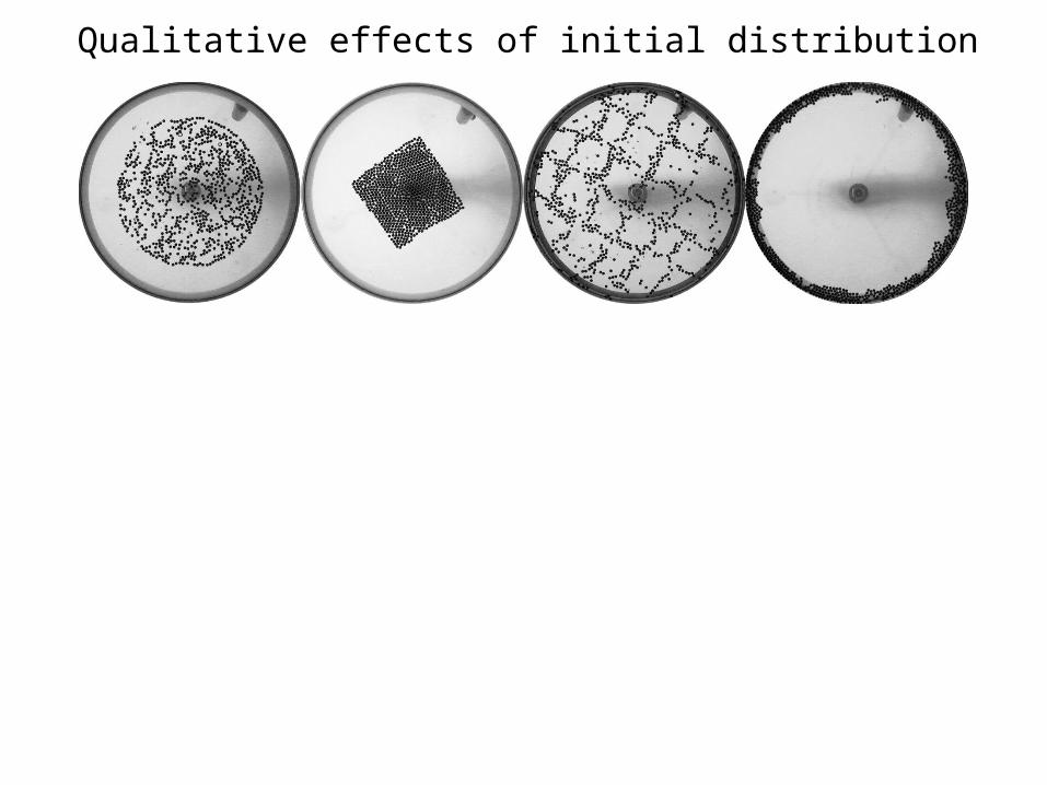
Qualitative effects of initial distribution
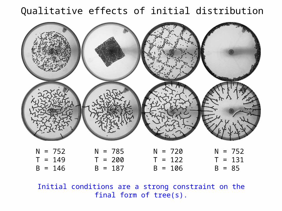
Qualitative effects of initial distribution
N = 752T = 131B = 85
N = 720T = 122B = 106
N = 785T = 200B = 187
N = 752T = 149B = 146
Initial conditions are a strong constraint on the final form of tree(s).
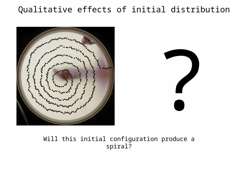
Qualitative effects of initial distribution
Will this initial configuration produce a spiral?
?
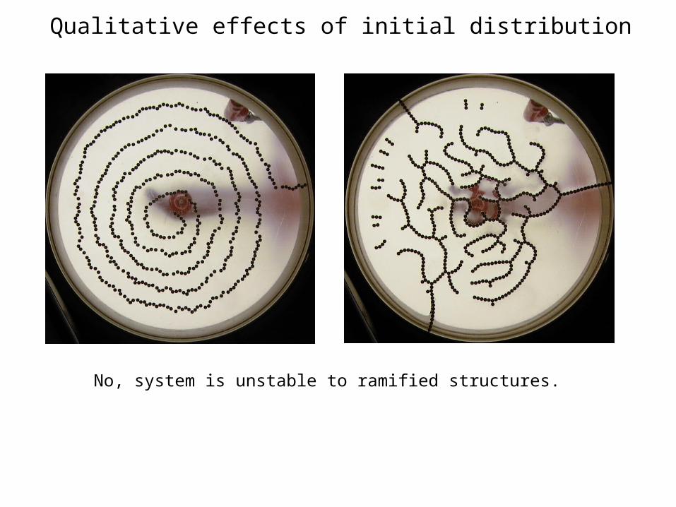
Qualitative effects of initial distribution
No, system is unstable to ramified structures.

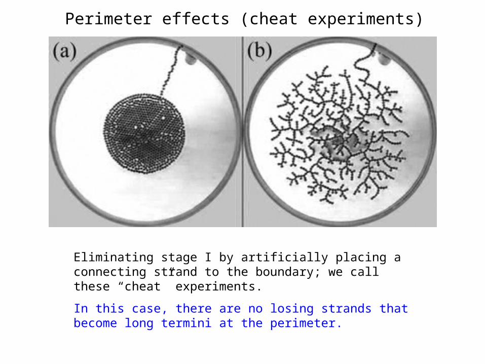
Perimeter effects (cheat experiments)
Eliminating stage I by artificially placing a connecting strand to the boundary; we call these “cheat” experiments.
Perimeter effects (cheat experiments)
Eliminating stage I by artificially placing a connecting strand to the boundary; we call these “cheat” experiments.
In this case, there are no losing strands that become long termini at the perimeter.
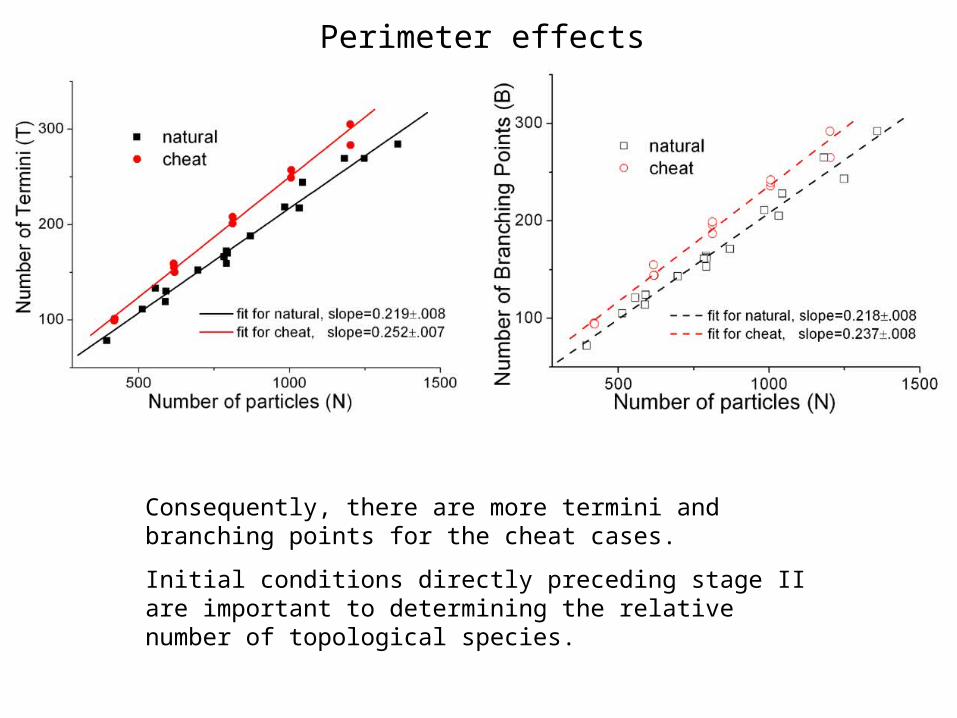
Perimeter effects
Consequently, there are more termini and branching points for the cheat cases.
Initial conditions directly preceding stage II are important to determining the relative number of topological species.
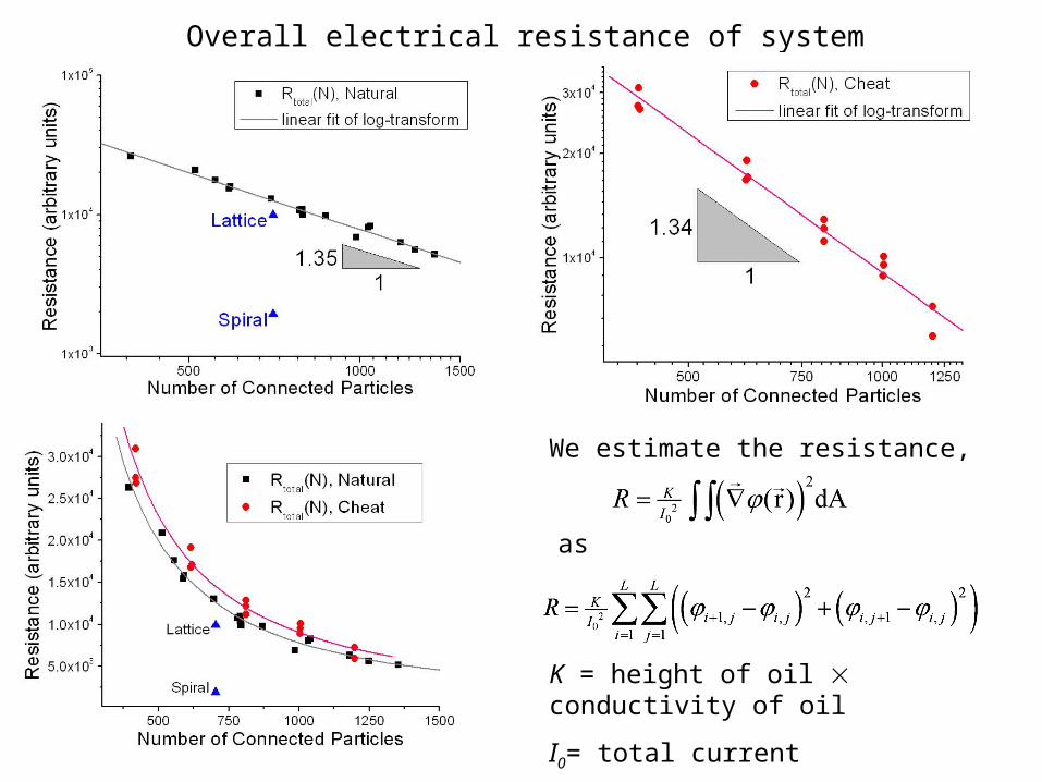
Overall electrical resistance of system
We estimate the resistance,
as
K = height of oil conductivity of oil
I0= total current

Review of experimental results
Growth of trees occurs in three stages.
Average adjacency captures the three stages.
Topology of network forms relatively quickly.
Particles become one of three species.
The relative abundance of each species is statistically
reproducible.
Initial conditions are a strong constraint to formation of
networks.
Artificially generated networks
How does the state of the system directly preceding stage II affect the topology of the trees?
Can we predict the final tree at this stage?
Artificially generated networks
Since topology of the networks is established relatively quickly, particles connect to one another before they have moved far.
Thus, we attempt to model the connections formed by the system using only the local information for each particle—it’s neighborhood.
Artificially generated networks
Since topology of the networks is established relatively quickly, particles connect to one another before they have moved far.
Thus, we attempt to model the connections formed by the system using only the local information for each particle—it’s neighborhood.We use data from the experiments: a snapshot of the particles directly preceding stage II.
Artificially generated networks
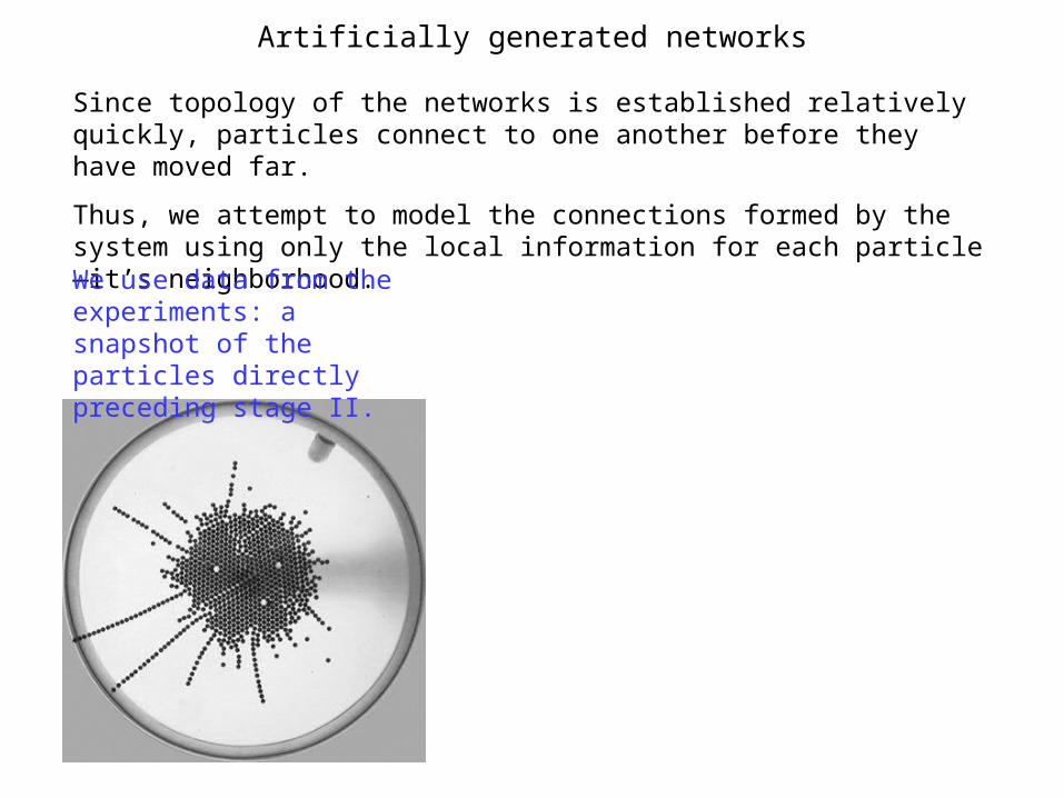
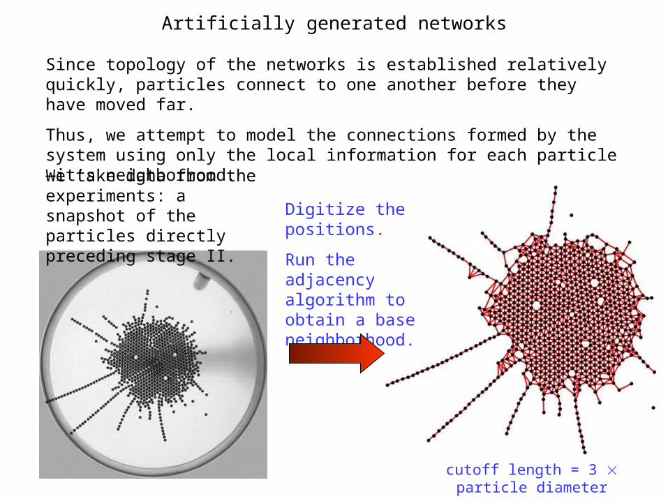
Since topology of the networks is established relatively quickly, particles connect to one another before they have moved far.
Thus, we attempt to model the connections formed by the system using only the local information for each particle—it’s neighborhood.We take data from the experiments: a snapshot of the particles directly preceding stage II.
Digitize the positions.
Run the adjacency algorithm to obtain a base neighborhood.
cutoff length = 3 particle diameter
Artificially generated networks
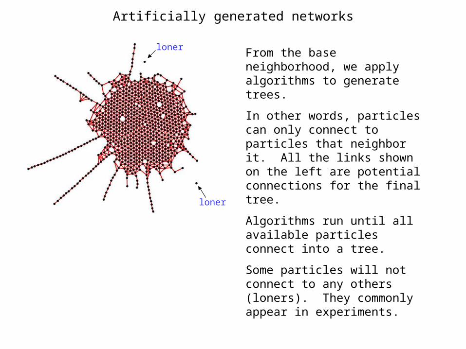
From the base neighborhood, we apply algorithms to generate trees.
In other words, particles can only connect to particles that neighbor it. All the links shown on the left are potential connections for the final tree.
Algorithms run until all available particles connect into a tree.
Some particles will not connect to any others (loners). They commonly appear in experiments.
loner
loner

Artificially generated networks
From the base neighborhood, we apply algorithms to generate trees.
In other words, particles can only connect to particles that neighbor it. All the links shown on the left are potential connections for the final tree.
Algorithms run until all available particles connect into a tree.
Some particles will not connect to any others (loners). They commonly appear in experiments.
We chose three algorithms to implement:
1) random (RAN)
2) minimum spanning tree (MST)
3) propagating front model (PFM)
loner
loner
Random
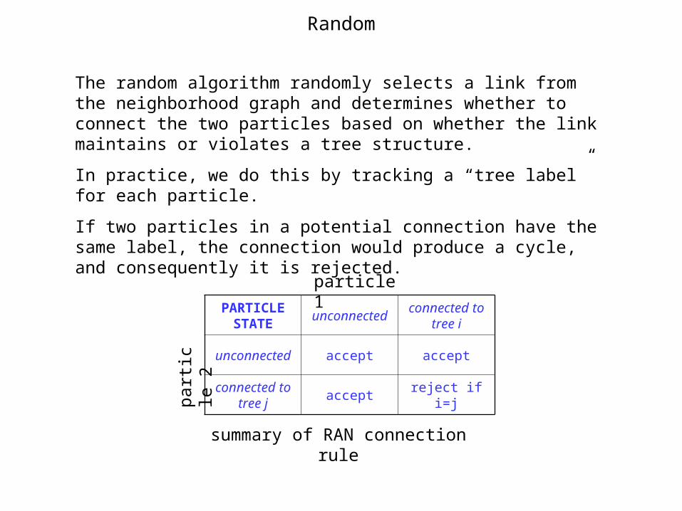
The random algorithm randomly selects a link from the neighborhood graph and determines whether to connect the two particles based on whether the link maintains or violates a tree structure.
In practice, we do this by tracking a “tree label” for each particle.
If two particles in a potential connection have the same label, the connection would produce a cycle, and consequently it is rejected.
PARTICLE STATE
unconnectedconnected to
tree i
unconnected accept accept
connected to tree j
accept reject if i=j
particle 1
part
icl
e 2
summary of RAN connection rule

RAN
movie of random algorithm
RAN
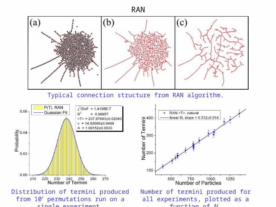
Typical connection structure from RAN algorithm.
Distribution of termini produced from 105 permutations run on a single
experiment.
Number of termini produced for all experiments, plotted as a function of
N.
Minimum Spanning Tree
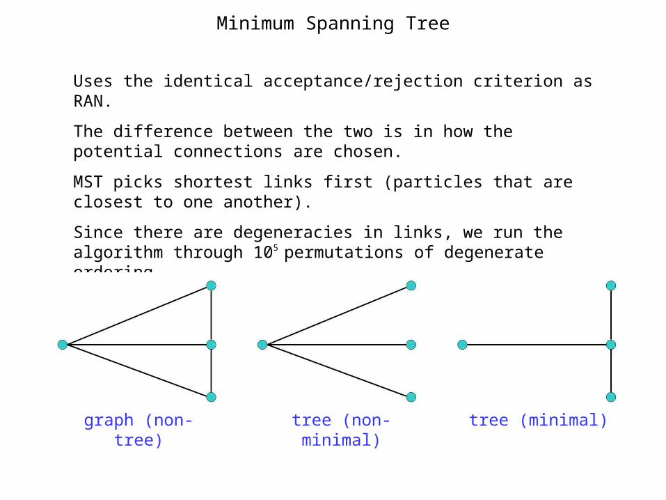
Uses the identical acceptance/rejection criterion as RAN.
The difference between the two is in how the potential connections are chosen.
MST picks shortest links first (particles that are closest to one another).
Since there are degeneracies in links, we run the algorithm through 105 permutations of degenerate ordering.
graph (non-tree) tree (non-minimal) tree (minimal)
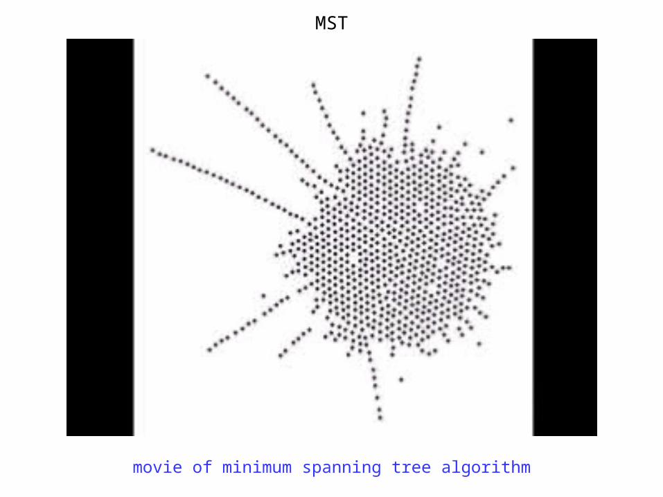
MST
movie of minimum spanning tree algorithm
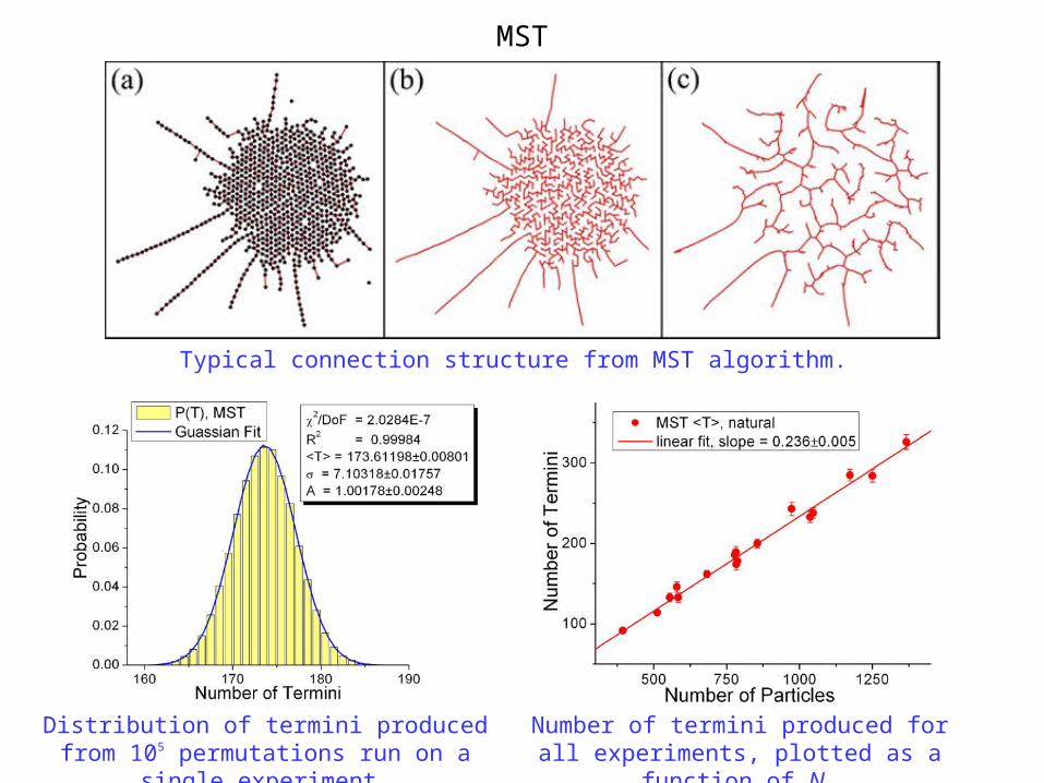
MST
Typical connection structure from MST algorithm.
Distribution of termini produced from 105 permutations run on a single
experiment.
Number of termini produced for all experiments, plotted as a function of
N.
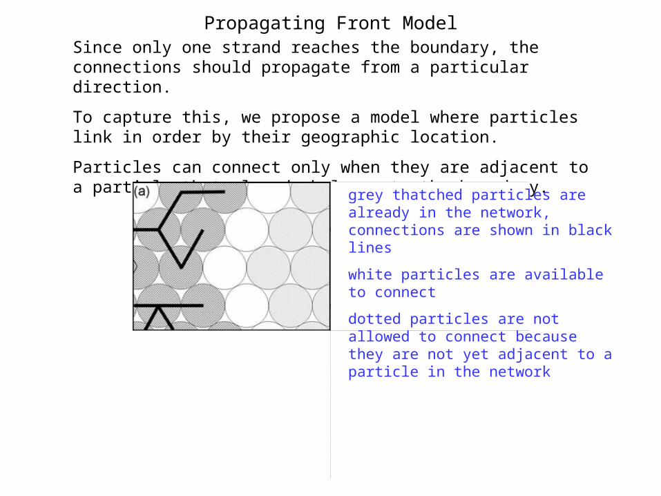
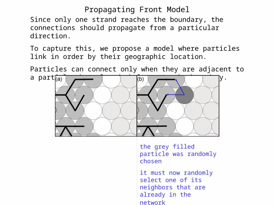
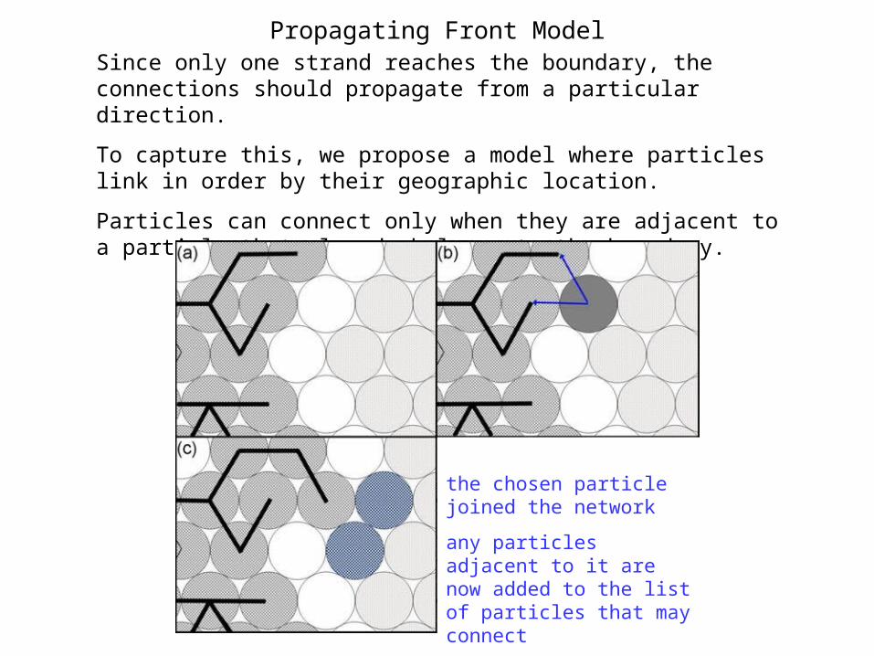
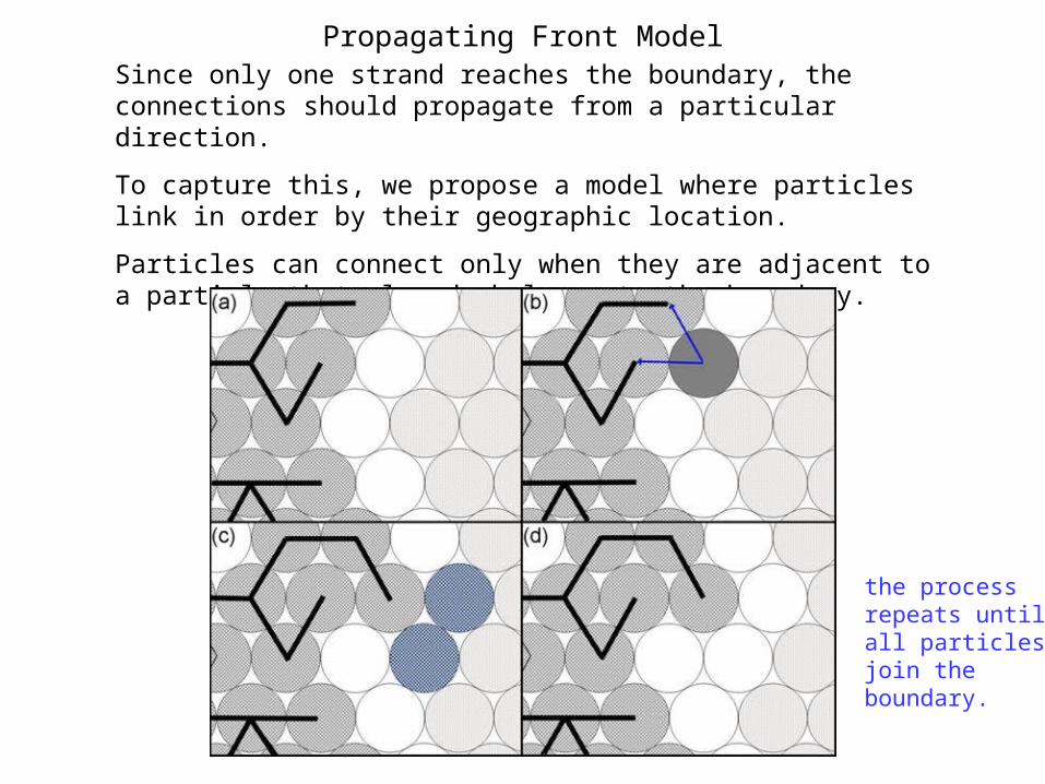
Propagating Front ModelSince only one strand reaches the boundary, the connections should propagate from a particular direction.
To capture this, we propose a model where particles link in order by their geographic location.
Particles can connect only when they are adjacent to a particle that already belongs to the boundary.
grey thatched particles are already in the network, connections are shown in black lines
white particles are available to connect
dotted particles are not allowed to connect because they are not yet adjacent to a particle in the network
Propagating Front ModelSince only one strand reaches the boundary, the connections should propagate from a particular direction.
To capture this, we propose a model where particles link in order by their geographic location.
Particles can connect only when they are adjacent to a particle that already belongs to the boundary.
the grey filled particle was randomly chosen
it must now randomly select one of its neighbors that are already in the network
Propagating Front ModelSince only one strand reaches the boundary, the connections should propagate from a particular direction.
To capture this, we propose a model where particles link in order by their geographic location.
Particles can connect only when they are adjacent to a particle that already belongs to the boundary.
the chosen particle joined the network
any particles adjacent to it are now added to the list of particles that may connect
Propagating Front ModelSince only one strand reaches the boundary, the connections should propagate from a particular direction.
To capture this, we propose a model where particles link in order by their geographic location.
Particles can connect only when they are adjacent to a particle that already belongs to the boundary.
the process repeats until all particles join the boundary.
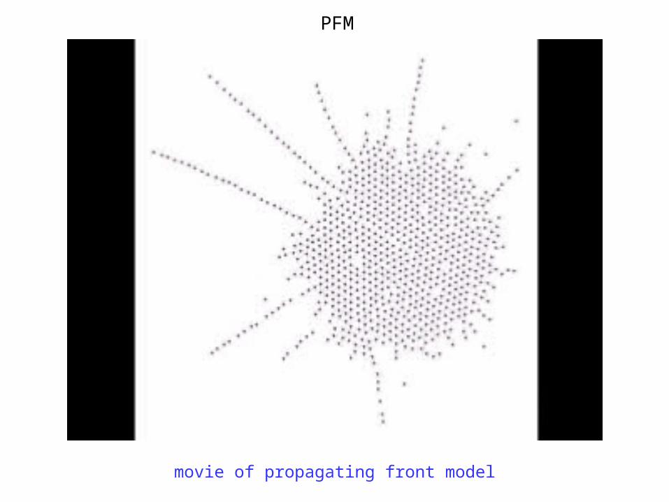
PFM
movie of propagating front model
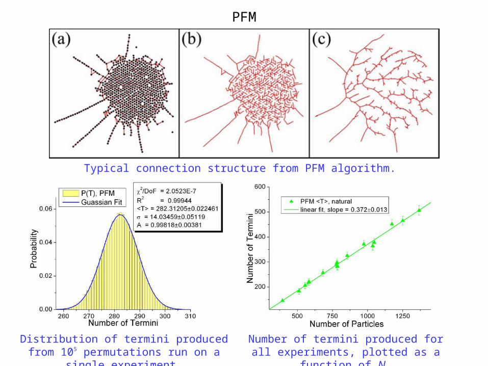
PFM
Typical connection structure from PFM algorithm.
Distribution of termini produced from 105 permutations run on a single
experiment.
Number of termini produced for all experiments, plotted as a function of
N.
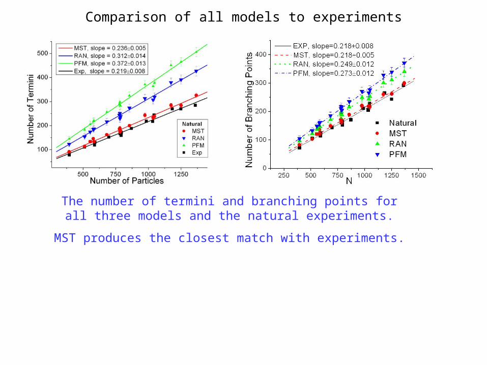
Comparison of all models to experiments
The number of termini and branching points for all three models and the natural experiments.
MST produces the closest match with experiments.
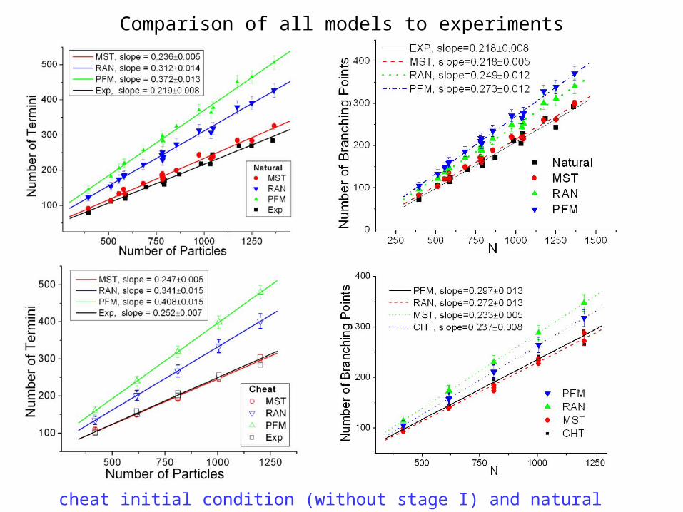
Comparison of all models to experiments
cheat initial condition (without stage I) and natural initial condition
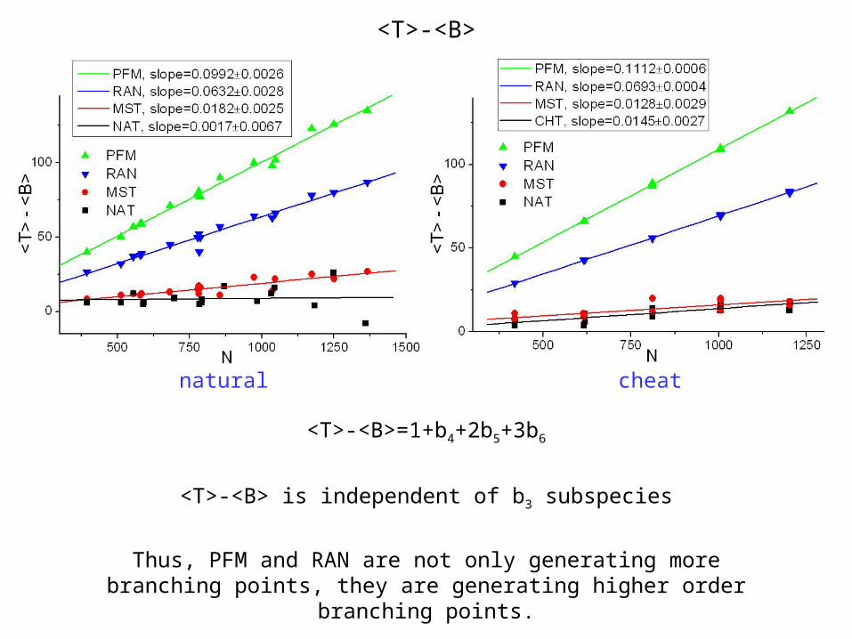
<T>-<B>
<T>-<B>=1+b4+2b5+3b6
<T>-<B> is independent of b3 subspecies
Thus, PFM and RAN are not only generating more branching points, they are generating higher order branching points.
natural cheat
Review of simulations
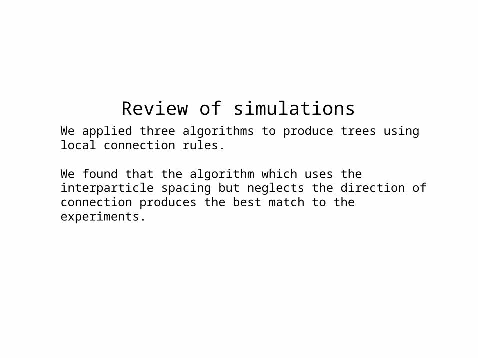
We applied three algorithms to produce trees using local connection rules.
We found that the algorithm which uses the interparticle spacing but neglects the direction of connection produces the best match to the experiments.
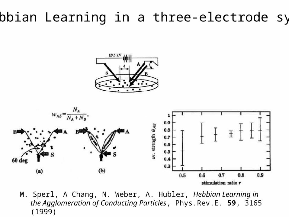
Hebbian Learning in a three-electrode system
M. Sperl, A Chang, N. Weber, A. Hubler, Hebbian Learning in the Agglomeration of Conducting Particles, Phys.Rev.E. 59, 3165 (1999)
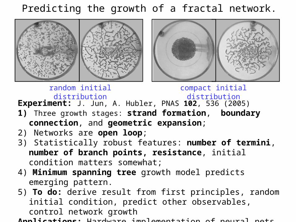
Predicting the growth of a fractal network.
Experiment: J. Jun, A. Hubler, PNAS 102, 536 (2005)1) Three growth stages: strand formation, boundary connection, and
geometric expansion;2) Networks are open loop;3) Statistically robust features: number of termini, number of branch
points, resistance, initial condition matters somewhat;4) Minimum spanning tree growth model predicts emerging pattern.5) To do: derive result from first principles, random initial condition, predict
other observables, control network growthApplications: Hardware implementation of neural nets, nano neural nets with
SC particles - M. Sperl, A Chang, N. Weber, A. Hubler, Hebbian Learning in the Agglomeration of Conducting Particles, Phys.Rev.E. 59, 3165 (1999)
random initial distribution compact initial distribution