
Self-adaptive mix of particle swarm methodologies for constrained optimization
18
Self-adaptive mix of particle swarm methodologies for constrained optimization Saber M. Elsayed a,⇑ , Ruhul A. Sarker a , Efrén Mezura-Montes b a School of Engineering and Information Technology, University of New South Wales at Canberra, Canberra 2600, Australia b Departamento de Inteligencia Artificial, Universidad Veracruzana, Sebastián Camacho 5, Centro, Xalapa, Veracruz 91000, Mexico article info Article history: Received 12 November 2012 Received in revised form 24 July 2013 Accepted 27 January 2014 Available online xxxx Keywords: Constrained optimization Particle swarm optimization Ensemble of operators abstract In recent years, many different variants of the particle swarm optimizer (PSO) for solving optimization problems have been proposed. However, PSO has an inherent drawback in handling constrained problems, mainly because of its complexity and dependency on parameters. Furthermore, one PSO variant may perform well for some test problems but not obtain good results for others. In this paper, our purpose is to develop a new PSO algo- rithm that can efficiently solve a variety of constrained optimization problems. It considers a mix of different PSO variants each of which evolves with a different number of individ- uals from the current population. In each generation, the algorithm assigns more individ- uals to the better-performing variants and fewer to the worse-performing ones. Also, a new PSO variant is developed for use in the proposed algorithm to maintain a better balance between its local and global PSO versions. A new methodology for adapting PSO parame- ters is presented and the proposed self-adaptive PSO algorithm tested and analyzed on two sets of test problems, namely the CEC2006 and CEC2010 constrained optimization problems. Based on the results, the proposed algorithm shows significantly better perfor- mance than the same global and local PSO variants as well as other-state-of-the-art algo- rithms. Although, based on our analysis, it cannot guarantee an optimal solution for any unknown problem, it is expected to be able to solve a wide variety of practical problems. Ó 2014 Elsevier Inc. All rights reserved. 1. Introduction Constrained optimization problems (COPs) are common in many real world applications and their purpose is to deter- mine the values for a set of decision variables by optimizing the objective function while satisfying the functional constraints and variable bounds as: min f ð X ! Þ s:t: : g k ð X ! Þ 6 0; k ¼ 1; 2; ... ; K h e ð X ! Þ¼ 0; e ¼ 1; 2; ... ; E L j 6 x j 6 U j j ¼ 1; 2; ... ; D ð1Þ http://dx.doi.org/10.1016/j.ins.2014.01.051 0020-0255/Ó 2014 Elsevier Inc. All rights reserved. ⇑ Corresponding author. Tel.: +61 425151130. E-mail addresses: [email protected] (S.M. Elsayed), [email protected] (R.A. Sarker), [email protected] (E. Mezura-Montes). Information Sciences xxx (2014) xxx–xxx Contents lists available at ScienceDirect Information Sciences journal homepage: www.elsevier.com/locate/ins Please cite this article in press as: S.M. Elsayed et al., Self-adaptive mix of particle swarm methodologies for constrained optimization, In- form. Sci. (2014), http://dx.doi.org/10.1016/j.ins.2014.01.051
Transcript of Self-adaptive mix of particle swarm methodologies for constrained optimization
Information Sciences xxx (2014) xxx–xxx
Contents lists available at ScienceDirect
Information Sciences
journal homepage: www.elsevier .com/locate / ins
Self-adaptive mix of particle swarm methodologies forconstrained optimization
http://dx.doi.org/10.1016/j.ins.2014.01.0510020-0255/� 2014 Elsevier Inc. All rights reserved.
⇑ Corresponding author. Tel.: +61 425151130.E-mail addresses: [email protected] (S.M. Elsayed), [email protected] (R.A. Sarker), [email protected] (E. Mezura-Montes).
Please cite this article in press as: S.M. Elsayed et al., Self-adaptive mix of particle swarm methodologies for constrained optimizatform. Sci. (2014), http://dx.doi.org/10.1016/j.ins.2014.01.051
Saber M. Elsayed a,⇑, Ruhul A. Sarker a, Efrén Mezura-Montes b
a School of Engineering and Information Technology, University of New South Wales at Canberra, Canberra 2600, Australiab Departamento de Inteligencia Artificial, Universidad Veracruzana, Sebastián Camacho 5, Centro, Xalapa, Veracruz 91000, Mexico
a r t i c l e i n f o a b s t r a c t
Article history:Received 12 November 2012Received in revised form 24 July 2013Accepted 27 January 2014Available online xxxx
Keywords:Constrained optimizationParticle swarm optimizationEnsemble of operators
In recent years, many different variants of the particle swarm optimizer (PSO) for solvingoptimization problems have been proposed. However, PSO has an inherent drawback inhandling constrained problems, mainly because of its complexity and dependency onparameters. Furthermore, one PSO variant may perform well for some test problems butnot obtain good results for others. In this paper, our purpose is to develop a new PSO algo-rithm that can efficiently solve a variety of constrained optimization problems. It considersa mix of different PSO variants each of which evolves with a different number of individ-uals from the current population. In each generation, the algorithm assigns more individ-uals to the better-performing variants and fewer to the worse-performing ones. Also, a newPSO variant is developed for use in the proposed algorithm to maintain a better balancebetween its local and global PSO versions. A new methodology for adapting PSO parame-ters is presented and the proposed self-adaptive PSO algorithm tested and analyzed ontwo sets of test problems, namely the CEC2006 and CEC2010 constrained optimizationproblems. Based on the results, the proposed algorithm shows significantly better perfor-mance than the same global and local PSO variants as well as other-state-of-the-art algo-rithms. Although, based on our analysis, it cannot guarantee an optimal solution for anyunknown problem, it is expected to be able to solve a wide variety of practical problems.
� 2014 Elsevier Inc. All rights reserved.
1. Introduction
Constrained optimization problems (COPs) are common in many real world applications and their purpose is to deter-mine the values for a set of decision variables by optimizing the objective function while satisfying the functional constraintsand variable bounds as:
min f ðX!Þ
s:t: : gkðX!Þ 6 0; k ¼ 1;2; . . . ;K
heðX!Þ ¼ 0; e ¼ 1;2; . . . ; E
Lj 6 xj 6 Uj j ¼ 1;2; . . . ;D
ð1Þ
ion, In-

2 S.M. Elsayed et al. / Information Sciences xxx (2014) xxx–xxx
where X!¼ ½x0; x1; . . . ; xD�T is a vector with D-decision variables, f ðX!Þ the objective function, gkðX
!Þ the kth inequality con-
straints, heðX!Þ the eth equality constraint and Lj and Uj the lower and upper limits of xj, respectively.
COPs are considered complex because of their unique structures and variations in mathematical properties. They maycontain different types of variables, such as real, integer and discrete, and have equality and/or inequality constraints. ACOP’s objective and constraint functions can be linear or nonlinear, continuous or discontinuous, and unimodal or multi-modal. Its feasible region can be either a tiny or significant portion of the search space and either one single bounded regionor a collection of multiple disjointed regions. Its optimal solution may exist either on the boundary of the feasible space or inthe interior of the feasible region. Also, high dimensionality due to their large numbers of variables and constraints may addfurther complexity to solving COPs.
Researchers and practitioners have attempted to use different computational intelligence methods to solve such prob-lems, such as PSO [25,36,38,49,53,56], genetic algorithms (GA) [19] and differential evolution (DE) [52]. PSO was conceivedas a simulation of the social behavior of flocks of birds and fishes [25] and is easy to both understand and implement. As aresult, during the last decade, it has become very popular and successfully applied for control problems [1,59,61] in the areasof image processing [40], mobile robot navigation [5], airfoil in transonic flow [43], and mechanical engineering [21]. How-ever, the choice of operators for any PSO algorithm plays a pivotal role in its success but is often made by trial and error.Because of the variability of the characteristics of optimization problems, most PSO algorithms may work well for one classof problems but it is not guaranteed to do so for another. To deal with this issue, as discussed later, an ensemble of evolu-tionary algorithms (EAs) and/or operator methodologies have recently been introduced [39].
Elsayed et al. [11] proposed a multi-topology PSO algorithm with a local search technique which was tested by solv-ing a small set of constrained problems. The algorithm produced very encouraging results that indicate it is worthy offurther investigation. Spanevello and de Oca [50] proposed two adaptive heterogeneous PSO algorithms for solvingoptimization problems. In the first, each particle counted the number of consecutive function evaluations in which itspersonal best did not improve. When the value of the counter exceeded pre-defined parameter values, the particleswitched its search mechanism and reset its counter. In the second, each particle adopted one mechanism based on aprobability and, at the same time, some of the particles were fixed to use a specific PSO strategy. However, the resultsobtained from solving a set of unconstrained problems showed that using the adaptive mechanisms hindered the algo-rithms’ performances. Engelbrecht [17] proposed a heterogeneous PSO algorithm for six unconstrained problems inwhich each particle randomly selected one of five PSO strategies. It demonstrated good performances in comparisonwith a single strategy PSO and also for large-scale problems [18] as well as dynamic problems [26]. However, no mech-anism for favoring the best-performing strategy was proposed. To deal with the abovementioned shortcoming, Nepo-muceno and Engelbrecht [37] introduced two new self-adaptive heterogeneous PSO algorithms which were influencedby the ant colony optimization meta-heuristic. They were tested on unconstrained problems, with the results showingthat the performances of both outranked those of other state-of-the-art algorithms. Wang et al. [58] introduced a self-adaptive learning-based PSO algorithm to tackle unknown landscapes in which a probability model was used to describethe probability of a strategy being used to update a particle which performed well on a set of unconstrained problems.Generally speaking, as the potential of ensemble methodologies in PSO to solve COPs has not fully been investigated in,this is our focus in this paper.
In the literature on ensemble operators, Qin et al. [45] proposed a DE algorithm that used two mutation strategies to oneof which each individual was assigned based on a given probability. After evaluating all the newly generated trial vectors, thenumbers of them successfully entered into the next generation were recorded as ns1 and ns2 and accumulated within a spec-ified number of generations called the ‘‘learning period’’. Then, the probability of assigning each individual was updated but,if it was zero, it might have been totally excluded from the list. Mallipeddi et al. [30] proposed an ensemble of mutationstrategies and control parameters with DE (EPSDE) for solving unconstrained optimization problems. In EPSDE, a pool of dis-tinct mutation strategies, along with a pool of values for each control parameter, coexisted throughout the evolution processand competed to produce offspring. Mallipeddi et al. [31] then extended their algorithm for constrained optimization by add-ing an ensemble of four constraint-handling techniques. Tasgetiren et al. [55] proposed an ensemble DE designed in such away that each individual was assigned to one of two distinct mutation strategies or a variable parameter search (VPS), withthe latter used to enhance the local exploitation capability. However, no adaptive strategy was used in their algorithm. El-sayed et al. [15] proposed a mix of four different DE mutation strategies within a single algorithm framework to solve COPswhich performed well for solving a set of small-scale theoretical benchmark constrained problems and was further extendedin [14,16]. Elsayed et al. [12] proposed two novel DE variants each of which utilized the strengths of multiple mutation andcrossover operators to solve 60 constrained problems and demonstrated competitive, if not better, performances in compar-ison with those of state-of-the-art algorithms. Spears [51] applied an adaptive strategy in a GA using two different crossoversfor solving N-peak problems. Eiben et al. [10] developed an adaptive GA framework with multiple crossover operators forsolving unconstrained problems in which the population was divided into a number of sub-populations, each of which useda particular crossover. Although, based on the success of these crossovers, the sub-population sizes were varied, their adap-tive GAs did not outperform the standard GA using only the best crossover. Hyun-Sook and Byung-Ro [23] investigatedwhether a combination of crossover operators could perform better than using only the best crossover operator by solvingthe traveling salesman problem (TSP) and graph bisection problem, with their adaptive strategy being to assign probabilitiesto using different crossovers.
Please cite this article in press as: S.M. Elsayed et al., Self-adaptive mix of particle swarm methodologies for constrained optimization, In-form. Sci. (2014), http://dx.doi.org/10.1016/j.ins.2014.01.051
S.M. Elsayed et al. / Information Sciences xxx (2014) xxx–xxx 3
Based on the above discussion, the key contributions made in this paper are:
(1) proposing an ensemble of different PSO variants for solving COPs;(2) introducing a self-adaptive mechanism to decide parameter values on which PSO is highly dependent; and(3) developing a new PSO variant with an archive that will maintain a balance between global and local PSO variants and,
thus, reduce the chance of solutions becoming stuck in local optima which occurs using other variants.
In the proposed ensemble algorithm, a set of different PSO variants are used each of which is considered to evolve differ-ent individuals in the current population and, at each generation, has an improvement index calculated for it. Based on thismeasure, the number of individuals assigned to each variant is determined adaptively while considering not discarding anyPSO variant during the evolution process when, at different stages, the performances of different variants may vary. Moreinterestingly, each individual in the population is assigned to three values, each representings one PSO parameter value,which are then evolved using a particle swarm variant. Generally speaking, this type of algorithm can be seen not only asa better alternative to a trial and error-based design but also a provider of better problem coverage.
To judge the performance of the proposed algorithm, a set of CEC2006 [27] and CEC2010 [33] constrained problems aresolved. Based on the quality of the solutions it obtains and computational times it requires, it demonstrates superior perfor-mance over other independent PSO variants as well as other state-of-the-art algorithms.
This paper is organized as follows. After this introduction, Section 2 presents an overview of PSO, Section 3 describes theproposed algorithm and its components, Section 4 presents the experimental results and analyses of them and, finally, con-clusions and proposed future work are discussed in Section 5.
2. Particle Swarm Optimization (PSO)
As a stochastic global optimization method, PSO takes inspiration from the motions of a flock of birds searching for food[25]. The algorithm starts with an initial population (particles) which fly through a problem’s hyperspace at given velocities,with each particle’s velocity updated at each generation based on its own and its neighbor’s experiences [9,29]. The move-ment of each particle then naturally evolves to an optimal or near-optimal solution.
2.1. Operators and parameters
In the PSO field, particles have been studied in two general types of neighborhoods: global and local. In the former, par-ticles move towards the best particle found so far which leads to the algorithm having a quick convergence pattern and,maybe becoming trapped in local optima. On the other hand, in the local PSO, each particle’s velocity is adjusted accordingto both its personal best and the best particle within its neighborhood. In this variant, most probably, the algorithm is able toescape from local solutions but may suffer from a slower convergence pattern [29].
These two variants can be stated as follows: in a D-dimensional search space, the position and velocity of particle-z arerepresented as vectors Xz and Vz, respectively. Let pbestxz ¼ ðx
pbestz;1 ; xpbest
z;2 ; . . . ; xpbestz;j ; . . . ; xpbest
z;D Þ andgbestx ¼ xgbest
1 ; xgbest2 ; . . . ; xgbest
j ; . . . ; xgbestD Þ be the best particle and the best position of its neighbors so far, respectively. Then,
its velocity and position/the particle in generation t can be calculated as:
(1) Global PSO:
Pleaseform.
Vtz;j ¼ wVt�1
z;j þ c1r1ðpbestxz;j � Xt�1z;j Þ þ c2r2ðgbestxj � xt
z;jÞ ð2Þ
(2) Local PSO:
Vtz;j ¼ wVt�1z;j þ c1r1;jðpbestxz;j � xt�1
z;j Þ þ c2r2;jðlbestxz;j � xtz;jÞ ð3Þ
xtz ¼ xt�1
z þ Vtz ð4Þ
where Vt�1z is the velocity of particle z at generation t � 1, Vz 2 ½�Vmax;Vmax�, w the inertia weight factor, c1 and c2 the accel-
eration coefficients, r1,j and r2,j the uniform random numbers within [0,1] and lbestxz the local best for individual z.Clerc and Kennedy [6] proposed an alternative version of PSO in which the velocity adjustment is given as:
Vtþ1z;j ¼ s Vt�1
z;j þ c1r1ðpbestxz;j � xt�1z;j Þ þ c2r2 gbestxj � Xt�1
z;j
� �� �ð5Þ
where s is the constriction factor, s ¼ 2j2�u�
ffiffiffiffiffiffiffiffiffiffiffiffiu2�4ujp and u = c1 + c2, u > 4. This version of PSO eliminates the parameter Vmax,
where s = 0.729 while c1 + c1 > 4 while other researchers have mentioned that c1 = c2 = 1.49445 is a good choice [11]. Also,because PSO has a nature of prematurely converging, Mezura-Montes and Flores-Mendoza [35] proposed a PSO with a dy-namic (deterministic) adaptation mechanism for both s and c2 that was designed to start with low-velocity values for someparticles and then increase them during the search process. They also assumed that not all particles adapted as some woulduse fixed values of those two parameters.
Motivated by the fact that an individual was not influenced by only the best performer among his neighbors, Mendeset al. [34] proposed making all individuals fully informed by each particle using information from all its neighbors rather
cite this article in press as: S.M. Elsayed et al., Self-adaptive mix of particle swarm methodologies for constrained optimization, In-Sci. (2014), http://dx.doi.org/10.1016/j.ins.2014.01.051
4 S.M. Elsayed et al. / Information Sciences xxx (2014) xxx–xxx
than just the best. Although their proposed algorithm was better than other state-of-the-art algorithms, it was not able toobtain consistent results over all the unconstrained problems tested.
Parsopoulos and Vrahatis [42] proposed a unified PSO variant that harnessed both local and global variants of PSO withthe aim of combining their exploration and exploitation abilities without imposing additional requirements in terms of func-tion evaluations.
For the purpose of handling multi-modal problems, Qu et al. [46] proposed a distance-based locally informed PSO whicheliminated the need to specify any niching parameter and enhanced the fine search ability of PSO. It used several local beststo guide each particle’s search and the neighborhoods were estimated in terms of Euclidean distances. The algorithm wastested on a set of unconstrained problems and showed superior performance in comparison with niching algorithms. How-ever, our empirical results showed that this algorithm is poor at handling constrained problems.
For the local PSO, different neighborhood structures may affect the performance of swarms, such as ring, wheel and ran-dom local topologies. In the ring topology, each particle is connected to two neighbors, in the wheel topology, individuals areisolated from one another and information is only communicated to a focal individual and, in the random topology, eachindividual obtains information from a random individual. To tackle with the premature convergence behavior of PSO, manyresearch studies were proposed [24,4,57–58].
2.2. Review of solving COPs by PSO
Over the last few years, PSO has gradually gained more attention in terms of solving COPs. Cagnina et al. [3] proposed ahybrid PSO for solving COPs. In their algorithm, they introduced different methods for update particle information and used adouble population and special shake mechanism to maintain diversity. Although the results were competitive, optimal solu-tions to several test problems could not be obtained. As mentioned earlier, Mezura-Montes and Flores-Mendoza [35] pro-posed a PSO with a dynamic adaptation of two different PSO parameters which was tested on 24 test problems. Althoughtheir proposed algorithm was better than others, it was not able to obtain optimal solutions on many occasions and its per-formance was not consistent. The PSO algorithm developed by Hu and Eberhart [22] started with a group of feasible solu-tions, with the feasibility function used to check the satisfaction of constraints achieved by the newly explored solutions,and all particles kept only the feasible solutions in their memories. The algorithm was tested on 11 test problems but theresults were not consistent. Liang and Suganthan [29] proposed a dynamic multi-swarm PSO with a constraint-handlingmechanism for solving COPs in which the sub-swarms were adaptively assigned to explore different constraints accordingto their difficulties. In addition, a sequential quadratic programming (SQP) method was altered to improve its local searchability. Although the algorithm showed superior performance to many other algorithms, it seems that its search capabilitieswere highly dependent on SQP. The algorithm of Pulido and Coello [44] used the feasibility rule to handle constraints as wellas a turbulence operator to improve its exploratory capability. However, the results obtained were not consistent. Renatoand Leandro dos Santos [48] introduced a PSO algorithm in which the accelerating coefficients of PSO were generated usinga Gaussian probability distribution. In addition, two populations were evolved, one for the variable vector and the other forthe Lagrange multiplier vector. However, their algorithm was not able to obtain optimal solutions over all runs. He and Wang[20] proposed a co-evolutionary PSO algorithm in which the notion of co-evolution was employed and two kinds of swarms,for evolutionary exploration and exploitation, as well as penalty factors were evolved. The algorithm was competitive withother algorithms for solving different engineering problems.
Motivated by multi-objective optimization techniques, Ray and Liew [47] proposed an effective multi-level information-sharing strategy within a swarm to handle single-objective, constrained and unconstrained optimization problems in whicha better-performer list (BPL) was generated by a multi-level Pareto ranking scheme which treated every constraint as anobjective, while the particles which were not in the BPL gradually congregated around their closest neighbor in the BPL.Zahara and Kao [60,15] proposed a PSO algorithm using a gradient repair method and constraint fitness priority-based rank-ing method which performed well on different test problems. Elsayed et al. [16] introduced a PSO algorithm, with a periodicmode for handling constraints, which made periodic copies of the search space when it started the run. It evidenced an im-proved search performance compared with those of conventional modes and other algorithms. Parsopoulos and Vrahatis[41] proposed a unified PSO version (which balanced the influences of the global and local search directions in a unifiedscheme) and used a penalty function technique to handle constraints. Cagnina et al. [2] proposed a PSO algorithm for solvingCOPs called CPSO in which each particle consisted of a D-dimensional real number vector. The particles were evaluated usinga fitness function that chose a feasible individual over an infeasible one and, of the infeasible particles, it preferred those thatwere closer to the feasible region. To determine the degree of infeasibility, CPSO saved the largest violation obtained for eachconstraint and, when a particle was detected as infeasible, added the amount of violation corresponding to that particle (nor-malized with respect to the largest violation recorded so far).
3. Self-adaptive mix of particle swarm methodologies
In this section, we describe a new self-adaptive parameter control method in PSO, a new PSO variant with an archive, ourproposed algorithm which uses a self-adaptive mix of PSO variants (SAM-PSO) and the constraint-handling technique usedin this research.
Please cite this article in press as: S.M. Elsayed et al., Self-adaptive mix of particle swarm methodologies for constrained optimization, In-form. Sci. (2014), http://dx.doi.org/10.1016/j.ins.2014.01.051
S.M. Elsayed et al. / Information Sciences xxx (2014) xxx–xxx 5
3.1. New self-adaptive parameter control
From the literature, it is known that PSO is highly dependent on its own parameters (s, c1 and c2). Although researchersusually use fixed parameters in each generation (t), one of our aims is to allow the algorithm to choose its own parameters.
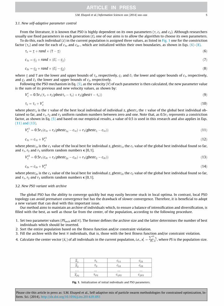
To do this, each individual (z) in the current population is assigned three values, as listed in Fig. 1 one for the constrictionfactor (sz) and one for each of c1z and c2z , which are initialized within their own boundaries, as shown in Eqs. (6)–(8).
Pleaseform.
sz ¼ sþ rand� ðs� sÞ ð6Þ
c1z ¼ c1 þ rand� ðc1 � c1Þ ð7Þ
c2z ¼ c2 þ rand� ðc2 � c2Þ ð8Þ
where s and s are the lower and upper bounds of sz, respectively, c1 and c1 the lower and upper bounds of c1, respectively,and c1 and c2 the lower and upper bounds of c2, respectively.
Following the PSO mechanism in Eq. (5), as the velocity (V) of each parameter is then calculated, the new parameter valueis the sum of its previous and new velocity values, as shown by:
Vsz ¼ 0:5r1ðsz þ r2ðpbestsz � szÞ þ r3ðgbests� szÞÞ ð9Þ
sz ¼ sz þ Vsz ð10Þ
where pbestsz is the s value of the best local individual of individual z, gbestsz the s value of the global best individual ob-tained so far, and r1, r2 and r3 uniform random numbers between zero and one. Note that, as 0.5r1 represents a constrictionfactor, as shown in Eq. (5) and based on our empirical results, a value of 0.5 is used in this research and also applies in Eqs.(11) and (13).
Vc1z ¼ 0:5r1ðc1z þ r2ðpbestc1z � c1zÞ þ r3ðgbestc1 � c1zÞÞ ð11Þ
c1z ¼ c1z þ Vc1z ð12Þ
where pbestc1z is the c1 value of the local best for individual z, gbestc1z the c1 value of the global best individual found so far,and r1, r2 and r3 uniform random numbers e [0,1].
Vc2z ¼ 0:5r1ðc2z þ r2ðpbestc2z � c2zÞ þ r3ðgbestc2 � c2zÞÞ ð13Þ
c2z ¼ c2z þ Vc2z ð14Þ
where pbestc2z is the c2 value of the local best for individual z, gbestc2z the c2 value of the global best individual found so far,and r1, r2 and r3 uniform random numbers e [0,1].
3.2. New PSO variant with archive
The global PSO has the ability to converge quickly but may easily become stuck in local optima. In contrast, local PSOtopology can avoid premature convergence but has the drawback of slower convergence. Therefore, it is beneficial to adopta new variant that can deal with this important issue.
Our method aims to maintain an archive of individuals which, to ensure a balance of intensification and diversification, isfilled with the best, as well as those far from the center, of the population, according to the following procedure.
1. Set two parameter values (PSarch and @). The former defines the archive size and the latter determines the number of bestindividuals which should be inserted.
2. Sort the entire population based on the fitness function and/or constraint violation.3. Fill the archive with the best @ individuals, that is, those with the best fitness function and/or constraint violation.
4. Calculate the center vector (~xc) of all individuals in the current population, i.e., xjc ¼
PPS
@ xi
PS�@ , where PS is the population size.
Fig. 1. Initialization of initial individuals and PSO parameters.
cite this article in press as: S.M. Elsayed et al., Self-adaptive mix of particle swarm methodologies for constrained optimization, In-Sci. (2014), http://dx.doi.org/10.1016/j.ins.2014.01.051
6 S.M. Elsayed et al. / Information Sciences xxx (2014) xxx–xxx
5. Calculate the Euclidian distance of each individual ðz;8@ < z 6 PSÞ to~xc , and then sort them from the largest to smallestdistance.
6. Add the best (PSarch � @) individual, based on its Euclidian distance, to the archive.7. Evolve all individuals using:
Pleaseform.
If rand < CFE=ðFFEs� 0:25FFEsÞVt
z ¼ szðVt�1z þ c1zr1ðpbestxz � xt�1
z Þ þ c2zr2ðxH � xt�1z ÞÞ ð15Þ
Else
Vtz;j ¼ szðVt�1
z;j þ c1zr1;jðpbestxz;j � xt�1z;j Þ þ c2zr2;jðxH;j � xt�1
z;j ÞÞ ð16Þ
~xtz ¼~xt�1
z þ V!t
z ð17Þ
where xH is selected from the archive pool, H is an integer random number e [1, w], and CFE and FFE the current and max-imum fitness evaluations, respectively. We must mention here that the difference between Eqs. (15) and (16) is that, in (15)H, r1 and r2 are fixed to update all variables while, in (16), for every j = 1, 2, . . . , D, a random H , r1 and r2 are selected. Fur-thermore, the algorithm places emphasis on (16) in the early stages of the search process to maintain diversity and thenadaptively focuses on (15).8. Gradually emphasize the best individuals and update w in the previous step as:� �
w ¼ PSarch � PSarch �CFEFFE
ð18Þ
We must mention here that the abovementioned steps 4 and 5 are discarded once w is less than @.
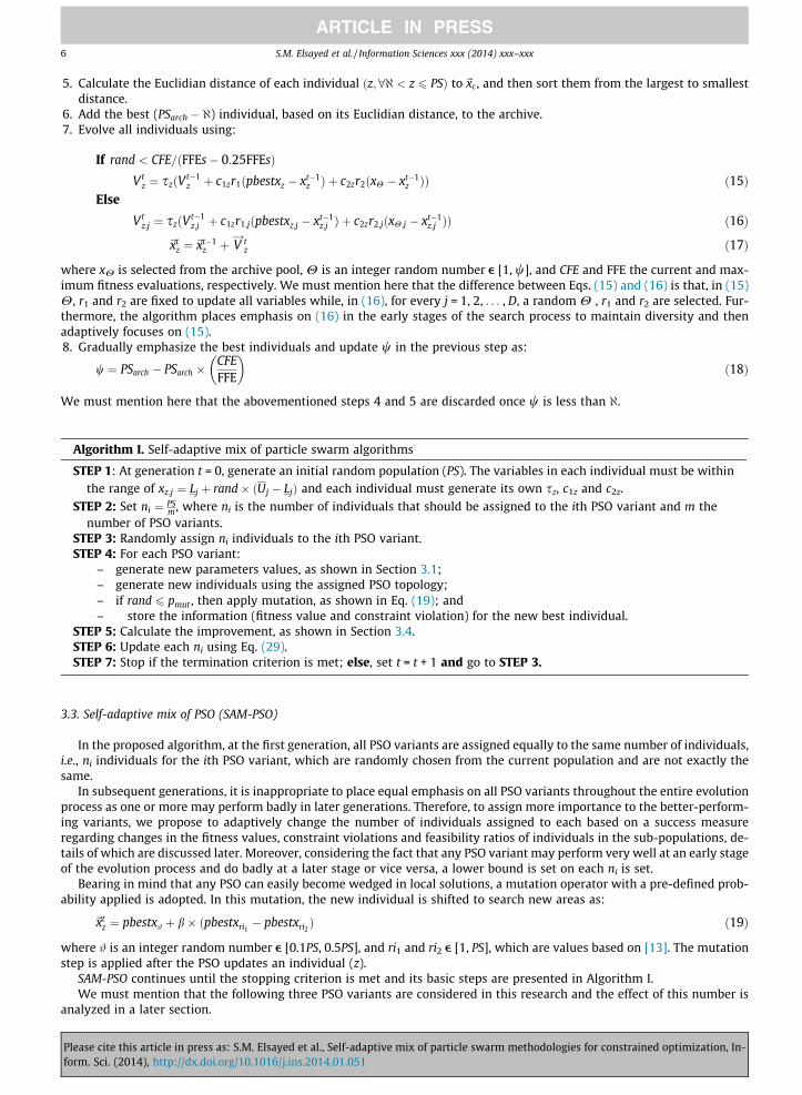
Algorithm I. Self-adaptive mix of particle swarm algorithms
STEP 1: At generation t = 0, generate an initial random population (PS). The variables in each individual must be withinthe range of xz;j ¼ Lj þ rand� ðUj � LjÞ and each individual must generate its own sz, c1z and c2z.
STEP 2: Set ni ¼ PSm, where ni is the number of individuals that should be assigned to the ith PSO variant and m the
number of PSO variants.STEP 3: Randomly assign ni individuals to the ith PSO variant.STEP 4: For each PSO variant:
– generate new parameters values, as shown in Section 3.1;– generate new individuals using the assigned PSO topology;– if rand 6 pmut , then apply mutation, as shown in Eq. (19); and– store the information (fitness value and constraint violation) for the new best individual.
STEP 5: Calculate the improvement, as shown in Section 3.4.STEP 6: Update each ni using Eq. (29).STEP 7: Stop if the termination criterion is met; else, set t = t + 1 and go to STEP 3.
3.3. Self-adaptive mix of PSO (SAM-PSO)
In the proposed algorithm, at the first generation, all PSO variants are assigned equally to the same number of individuals,i.e., ni individuals for the ith PSO variant, which are randomly chosen from the current population and are not exactly thesame.
In subsequent generations, it is inappropriate to place equal emphasis on all PSO variants throughout the entire evolutionprocess as one or more may perform badly in later generations. Therefore, to assign more importance to the better-perform-ing variants, we propose to adaptively change the number of individuals assigned to each based on a success measureregarding changes in the fitness values, constraint violations and feasibility ratios of individuals in the sub-populations, de-tails of which are discussed later. Moreover, considering the fact that any PSO variant may perform very well at an early stageof the evolution process and do badly at a later stage or vice versa, a lower bound is set on each ni is set.
Bearing in mind that any PSO can easily become wedged in local solutions, a mutation operator with a pre-defined prob-ability applied is adopted. In this mutation, the new individual is shifted to search new areas as:
~xtz ¼ pbestx# þ b� ðpbestxri1
� pbestxri2Þ ð19Þ
where # is an integer random number e [0.1PS, 0.5PS], and ri1 and ri2 e [1, PS], which are values based on [13]. The mutationstep is applied after the PSO updates an individual (z).
SAM-PSO continues until the stopping criterion is met and its basic steps are presented in Algorithm I.We must mention that the following three PSO variants are considered in this research and the effect of this number is
analyzed in a later section.
cite this article in press as: S.M. Elsayed et al., Self-adaptive mix of particle swarm methodologies for constrained optimization, In-Sci. (2014), http://dx.doi.org/10.1016/j.ins.2014.01.051

S.M. Elsayed et al. / Information Sciences xxx (2014) xxx–xxx 7
1. PSO with an archive, as described in Section 3.2.2. The local PSO with the aim of maintaining diversity.3. A sub-swarm PSO [29] in which all individuals are divided into one of five different sub-swarms. Each individual, except
the best (leader), in each sub-swarm is updated as:
Pleaseform.
Vtz;j ¼ szðVt�1
z;j þ c1zr1;jðpbestxz;j � xt�1z;j Þ þ c2zr2;jðpbestxx;j � xt�1
z;j ÞÞ ð20Þ
~xtz ¼~xt�1
z þ V!t
z ð21Þ
where pbestxx is the local best of a random x within the same sub-swarm.
The best particle (leader) in each sub-swarm is then updated using information about a random best particle in anothersub-swarm as:
Vtz;j ¼ szðVt�1
z;j þ c1zr1;jðpbestxz;j � xt�1z;j Þ þ c2zr2;jðpbestxh;j � xt�1
z;j ÞÞ ð22Þ
~xtz ¼~xt�1
z þ V!t
z ð23Þ
where pbestxh is the local best of a random best h individual in the other sub-swarms.
3.4. Improvement measure
To measure the improvement in each variant in a given generation, we consider both its feasibility status and fitness va-lue as it is always better to consider any improvement in feasibility than in infeasibility. For any generation (t > 1), one of thefollowing four scenarios arises.
(1) Infeasible to infeasible: for any variant (i), if the best solution is infeasible in generation t � 1 and still infeasible ingeneration t, the improvement index is calculated as:
Vi;t ¼jViobest
i;t � Viobesti;t�1j
avg � Vioi;t¼ Ii;t ð24Þ
where Viobesti;t is the constraints violation of the best individual in generation t and avg � Vioi,t the average violation. Therefore,
VIi,t = Ii,t represents the relative improvement compared with the average violation in the current generation.
(2) Feasible to feasible: for any variant (i), if the best solution is feasible in generation t � 1 and still feasible in generationt, the improvement index is:
Ii;t ¼ maxiðVIi;tÞ þ jFbest
i;t � Fbesti;t�1j � FRi;t ð25Þ
where Ii,t is the improvement for a PSO variant (i) in generation t, Fbesti;t the objective function for the best individual in gen-
eration t, and the feasibility ratio of variant i in generation t is:
FRi;t ¼Number of feasible solutions in a subpopulation i
Subpopulation size at iteration tð26Þ
To assign a higher index value to a PSO variant with a higher feasibility ratio, we multiply the improvement in fitnessvalue by the feasibility ratio. To differentiate between the improvement indices of feasible and infeasible groups of indi-viduals, we add a term (maxi(VIi,t)) to (25). If all the best solutions are feasible, maxiðVIi;tÞ will be zero.
(3) Infeasible to feasible: for any variant (i,) if the best solution is infeasible in both generation t � 1 and generation t, theimprovement index is:
Ii;t ¼ maxiðVIi;tÞ þ jVbest
i;t�1 þ Fbesti;t � Fbv
i;t�1j � FRi;t ð27Þ
where Fbvi;t�1 is the fitness value of the least violated individual in generation t � 1.
To assign a higher index value to an individual that changes from infeasible to feasible, we add Vbesti;t�1 to the change of
fitness value in (27).
cite this article in press as: S.M. Elsayed et al., Self-adaptive mix of particle swarm methodologies for constrained optimization, In-Sci. (2014), http://dx.doi.org/10.1016/j.ins.2014.01.051
8 S.M. Elsayed et al. / Information Sciences xxx (2014) xxx–xxx
(4) Becoming worse: considering the fitness function and/or constraint violation for any variant (i), if it becomes inferiorin generation (t) to its previous value in generation t � 1, the improvement index is:
Table 1Summa
Vari
Globadap
ParaPS =FFE =
Table 2Compar
Algo
sa-g-
Pleaseform.
Ii;t ¼ 0 ð28Þ
After calculating the improvement index for each PSO variant, the number of individuals assigned to each variant is calcu-lated according to:
ni;t ¼ MSSþ Ii;tPmi¼1 Ii;t
� ðPS�MSS� NoptÞ ð29Þ
where ni,t is the number of individuals assigned to the ith variant at generation t, MSS the minimum size of each i at gener-ation t, PS the total population size and Nopt the number of PSO variants.
3.5. Constraint handling
In this paper, constraints are handled as follows [8]: (i) between two feasible solutions, the fittest (according to the fitnessfunction) is better; (ii) a feasible solution is always better than an infeasible one; and (iii) between two infeasible solutions,the one with the smaller sum of constraint violations is preferred. The equality constraints are also transformed to inequal-ities of the following form, where e is a small value (here is equal to 0.0001):
jheð~xÞj � e 6 0; for e ¼ 1; . . . ; E ð30Þ
4. Experimental results
In this section, the performances of different components of the proposed algorithm are presented and analyzed bysolving 24 benchmark problems, the characteristics of which can be found in [27]. However, as all the algorithms con-sidered in this paper were not able to obtain feasible solutions for g20 and g22, we exclude them from ourexperiments.
All algorithms were coded using Matlab and run on a PC with a 3 GHz Core 2 Duo processor, 3.5 G RAM and Windows XP.
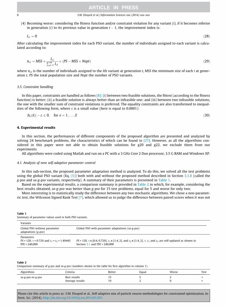
4.1. Analysis of new self-adaptive parameter control
In this sub-section, the proposed parameter adaptation method is analyzed. To do this, we solved all the test problemsusing the global PSO variant (Eq. (5)) both with and without the proposed method described in Section 3.1.1 (called theg-pso and sa-g-pso variants, respectively). A summary of their parameters is presented in Table 1.
Based on the experimental results, a comparison summary is provided in Table 2 in which, for example, considering thebest results obtained, sa-g-pso was better than g-pso for 15 test problems, equal for 5 and worse for only two.
More interesting is to statistically study the difference between any two stochastic algorithms. We chose a non-paramet-ric test, the Wilcoxon Signed Rank Test [7], which allowed us to judge the difference between paired scores when it was not
ry of parameter values used in both PSO variants.
ants
al PSO without parametertations (g-pso)
Global PSO with parameter adaptations (sa-g-pso)
meters120, s = 0.729 and c1 = c2 = 1.49445 PS = 120, s e [0.4, 0.729], c1 e [1.4, 2], and c2 e [1.4, 2], s, c1 and c2 are self-updated as shown in
Section 3.1 and FFE = 240,000240,000
ison summary of g-pso and sa-g-pso (numbers shown in the table for first algorithm in column 1).
rithms Criteria Better Equal Worse Test
pso-to-g-pso Best results 15 5 2 +Average results 19 2 0 +
cite this article in press as: S.M. Elsayed et al., Self-adaptive mix of particle swarm methodologies for constrained optimization, In-Sci. (2014), http://dx.doi.org/10.1016/j.ins.2014.01.051

S.M. Elsayed et al. / Information Sciences xxx (2014) xxx–xxx 9
possible to make the assumptions required by the t test, such as that the population should be normally distributed. Theresults based on the best and average fitness values are presented in the last column in Table 2. As a null hypothesis, it isassumed that there is no significant difference between the best and/or mean values of two samples whereas the alternativehypothesis is that there is a significant difference at a 5% significance level. Based on the test results, we assigned one ofthree signs (+, �, and �) for the comparison of any two algorithms (shown in the last two rows), where ‘+’ means thatsa-g-pso is significantly better than the other algorithm, ’�’ sign means that it is significantly worse and ‘�’ sign meansthat there is no significant difference between the two. From Table 2, it is clear that sa-g-pso was statistically superior tog-pso.
Considering the feasibility ratio results for sa-g-pso and g-pso of 90% and 86% feasibility ratios, respectively, sa-g-pso wasstill better.
In the previous analysis, we demonstrated that sa-g-pso achieved better quality solutions than g-pso. However, it isimportant to report their computational times. To test this, we compared that taken by each algorithm to reach the best-known solution with an error of 0.0001, i.e., the stopping criteria were ½f ð~xÞ � f ð~x�Þ 6 0:0001�, where f ð~x�Þ was the best-known solution and it was found that sa-g-pso took 49.8% less computational time than g-pso.
As further analysis required some convergence plots to illustrate the benefit of the proposed technique, two sample plotsare presented in Fig. 2, which clearly show that sa-g-pso was able to converge faster than g-pso. The algorithms’ perfor-mances on the remaining test problems were similar to those presented in these two plots.
4.2. Analysis of proposed PSO variant with archive
In this sub-section, an analysis of the proposed PSO with an archive discussed in Section 3.2, called pso-w-archive, isundertaken by comparing its performance with those of both a global and local PSO variant (sa-g-pso and sa-l-pso,respectively).
To begin with, the proposed self-adaptive mechanism is used to update the PSO parameters in all variants. Then, twomore parameters, PSarch = PS/2 and @ ¼ PS=3, are added to pso-w-archive the values of which are based on our empiricalresults.
(a) g01 (the y-axis is in the log scale) (b) g07 (the x-axis is in the log scale)
Fig. 2. Convergence plots of g-pso and sa-g-pso for (a) g01 and (b) g07.
Table 3Comparison summary of pso-w-archive against sa-g-pso and sa-l-pso.
Algorithms Criteria Better Equal Worse Test
pso-w-archive-to-sa-g-pso Best results 13 9 0 +Average results 15 7 0 +
pso-w-archive-to-sa-l-pso Best results 15 7 0 +Average results 14 7 1 +
Please cite this article in press as: S.M. Elsayed et al., Self-adaptive mix of particle swarm methodologies for constrained optimization, In-form. Sci. (2014), http://dx.doi.org/10.1016/j.ins.2014.01.051
10 S.M. Elsayed et al. / Information Sciences xxx (2014) xxx–xxx
Detailed results are shown in Appendix A and a comparison summary presented in Table 3 in which it is clear that, boththe best and average results of pso-w-archive were better than those of sa-g-pso and sa-l-pso, as confirmed by the Wilcoxontest pso-w-archive was statistically better.
More interestingly, pso-w-archive was able to obtain a 100% feasibility ratio while sa-g-pso and sa-l-pso reached 90% and70%, respectively.
Using the abovementioned measure to calculate the average computational time, compared with those of sa-g-pso and sa-l-pso, pso-w-archive was able to achieve savings of 7.05% and 10.36%, respectively.
4.3. Analysis of SAM-PSO
In this sub-section, to further analyze the proposed SAM-PSO, we compare its performance firstly against its independentvariants and then against state-of-the-art algorithms.
To begin with, SAM-PSO uses the same parameter settings as previously as well as two extra ones: MSS = 10%, as in [15];and the mutation rate (mr) set at 0.2.
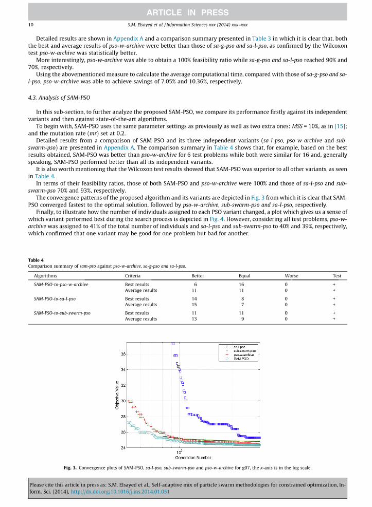
Detailed results from a comparison of SAM-PSO and its three independent variants (sa-l-pso, pso-w-archive and sub-swarm-pso) are presented in Appendix A. The comparison summary in Table 4 shows that, for example, based on the bestresults obtained, SAM-PSO was better than pso-w-archive for 6 test problems while both were similar for 16 and, generallyspeaking, SAM-PSO performed better than all its independent variants.
It is also worth mentioning that the Wilcoxon test results showed that SAM-PSO was superior to all other variants, as seenin Table 4.
In terms of their feasibility ratios, those of both SAM-PSO and pso-w-archive were 100% and those of sa-l-pso and sub-swarm-pso 70% and 93%, respectively.
The convergence patterns of the proposed algorithm and its variants are depicted in Fig. 3 from which it is clear that SAM-PSO converged fastest to the optimal solution, followed by pso-w-archive, sub-swarm-pso and sa-l-pso, respectively.
Finally, to illustrate how the number of individuals assigned to each PSO variant changed, a plot which gives us a sense ofwhich variant performed best during the search process is depicted in Fig. 4. However, considering all test problems, pso-w-archive was assigned to 41% of the total number of individuals and sa-l-pso and sub-swarm-pso to 40% and 39%, respectively,which confirmed that one variant may be good for one problem but bad for another.
Table 4Comparison summary of sam-pso against pso-w-archive, sa-g-pso and sa-l-pso.
Algorithms Criteria Better Equal Worse Test
SAM-PSO-to-pso-w-archive Best results 6 16 0 +Average results 11 11 0 +
SAM-PSO-to-sa-l-pso Best results 14 8 0 +Average results 15 7 0 +
SAM-PSO-to-sub-swarm-pso Best results 11 11 0 +Average results 13 9 0 +
Fig. 3. Convergence plots of SAM-PSO, sa-l-pso, sub-swarm-pso and pso-w-archive for g07, the x-axis is in the log scale.
Please cite this article in press as: S.M. Elsayed et al., Self-adaptive mix of particle swarm methodologies for constrained optimization, In-form. Sci. (2014), http://dx.doi.org/10.1016/j.ins.2014.01.051

Fig. 4. Example of self-adaptive change in number of individuals assigned to each PSO variant for g02 (x-axis represents generation number and y-axispopulation size).
Table 5Comparison summary of SAM-PSO against CPSO-SHAKE, IPSO, SAMO-GA, SAMO-DE and ECHT-EP2.
Algorithms Criteria Better Equal Worse Test
SAM-PSO-to-CPSO-shake Best results 9 13 0 +Average results 16 5 1 +
SAM-PSO-to-IPSO Best results 13 9 0 +Average results 15 7 0 +
SAM-PSO-to-SAMO-GA Best results 2 19 1Average results 14 8 0 +
SAM-PSO-to-SAMO-DE Best results 1 20 1 �Average results 8 13 1 +
SAM-PSO-to-ECHT-EP2 Best results 2 20 0 �Average results 4 16 2 �
Table 6Comparison summary of SAM-PSO against eDEag and CO-CLPSO.
D Comparison Fitness Better Equal Worse Test
10D SAM-PSO-to-eDEag Best 6 6 6 �Average 4 13 1 �
SAM-PSO-to-CO-CLPSO Best 14 3 1 +Average 15 0 3 +
30D SAM-PSO-to-eDEag Best 16 1 1 +Average 13 0 5 +
SAM-PSO-to-CO-CLPSO Best 17 1 0 +Average 17 0 1 +
S.M. Elsayed et al. / Information Sciences xxx (2014) xxx–xxx 11
4.4. SAM-PSO against state-of-the-art algorithms
Here, the results obtained by SAM-PSO are compared with those from other PSO state-of-the-art algorithms, namely theconstrained PSO with a shake mechanism (CPSO-shake) [3] and improved PSO (IPSO) [35], and other algorithms that useensembles of operators and/or constraint-handling techniques, that is, the self-adaptive multi-operators GA and DE,SAMO-GA [15] and SAMO-DE [15], respectively, and the ensemble of constraint-handling techniques based on evolutionaryprogramming (ECHT-EP2) [32]. We must mention that SAM-PSO and three other algorithms (SAMO-GA [15], SAMO-DE and
Please cite this article in press as: S.M. Elsayed et al., Self-adaptive mix of particle swarm methodologies for constrained optimization, In-form. Sci. (2014), http://dx.doi.org/10.1016/j.ins.2014.01.051
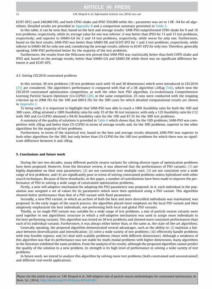
12 S.M. Elsayed et al. / Information Sciences xxx (2014) xxx–xxx
ECHT-EP2) used 240,000 FFE, and both CPSO-shake and IPSO 350,000 while the e parameter was set to 1.0E�04 for all algo-rithms. Detailed results are provided in Appendix B and a comparison summary presented in Table 5.
In this table, it can be seen that, based on the best and average results: SAM-PSO outperformed CPSO-shake for 9 and 16test problems, respectively, while its average value for one was inferior; it was better than IPSO for 13 and 15 test problems,respectively; and superior to SAMO-GA for 2 and 14 test problems, respectively, while worse for only one. Furthermore,based on the best results, SAM-PSO was better than SAMO-DE and ECHT-EP2 for 1 and 2 test problems, respectively, whileinferior to SAMO-DE for only one and, considering the average results, inferior to ECHT-EP2 for only two. Therefore, generallyspeaking, SAM-PSO performed better for the majority of the test problems.
Furthermore, the results from the Wilcoxon test proved that SAM-PSO was statistically better than both COPS-shake andIPSO and, based on the average results, better than SAMO-GA and SAMO-DE while there was no significant difference be-tween it and ECHT-EP2.
4.5. Solving CEC2010 constrained problems
In this section, 36 test problems (18 test problems each with 10 and 30 dimensions) which were introduced in CEC2010[33] are considered. The algorithm’s performance is compared with that of a DE algorithm (eDEag [54]), which won theCEC2010 constrained optimization competition, as well the other best PSO algorithm, Co-evolutionary ComprehensiveLearning Particle Swarm Optimizer (Co-CLPSO) [28], in the same competition. 25 runs were conducted with the stoppingcriterion up to 200K FEs for the 10D and 600 K FEs for the 30D cases for which detailed computational results are shownin Appendix C.
To being with, it is important to highlight that SAM-PSO was able to reach a 100% feasibility ratio for both the 10D and30D cases, eDEag attained a 100% feasibility ratio for only 35 of the 36 test instances, with only a 12% feasibility ratio for C12with 30D and Co-CLPSO obtained a 94.4% feasibility ratio for the 10D and 87.3% for the 30D test problems.
A summary of the quality of solutions is provided in Table 6 which shows that, for the 10D problems, SAM-PSO was com-petitive with eDEag and better than CO-CLPSO in terms of average results and, for the 30D problems, superior to the otheralgorithms for the majority of test problems.
Furthermore, in terms of the statistical test, based on the best and average results obtained, SAM-PSO was superior toboth other algorithms for the 30D, but only better than CO-CLPSO for the 10D test problems for which there was no signif-icant difference between it and eDEag.
5. Conclusions and future work
During the last two decades, many different particle swarm variants for solving diverse types of optimization problemshave been proposed. However, from the literature review, it was observed that the performances of PSO variants: (1) arehighly dependent on their own parameters; (2) are not consistent over multiple runs; (3) are not consistent over a widerange of test problems; and (4) are significantly poor in terms of solving constrained problems unless hybridized with othersearch techniques. Because of these drawbacks, in this paper, a number of contributions have been made to improve the per-formance of PSO in solving a wide range of constrained optimization problems.
Firstly, a new self-adaptive mechanism for adapting the PSO parameters was proposed. In it, each individual in the pop-ulation was assigned a set of values for its parameters which were then optimized using a PSO variant. This algorithmshowed better performance than that of a PSO variant with fixed parameters.
Secondly, a new PSO variant, in which an archive of both the best and more diversified individuals was maintained, wasproposed. In the early stages of the search process, the algorithm placed more emphasis on the local PSO variant and thenadaptively emphasized the best individuals, out-performing both local and global PSO variants.
Thirdly, as no single PSO variant was suitable for a wide range of test problems, a mix of particle swarm variants wereused together in one algorithmic structure in which a self-adaptive mechanism was used to assign more individuals tothe best-performing variants. This algorithm was tested on 58 test problems and showed more consistent performances thaneach of its individual variants. Furthermore, it was always either better than, or the same as, the state-of-the-art algorithms.
Generally speaking, the proposed algorithm demonstrated several advantages, such as the ability to: (i) maintain a bal-ance between diversification and intensification; (ii) solve a wide variety of test problems; (iii) effectively handle problemswith tiny feasible regions; and (iv) deal with scalable problems (those with different dimensions). Although a weakness ofthis algorithm was that its performance was not stable for multi-modal problems with higher dimensions, many algorithmsin the literature exhibited the same problem. From the analysis of its results, although the proposed algorithm cannot predictthe quality of the solution to a new problem, its strength is its high level of performance in solving a wide variety of testproblems.
In future work, we intend to analyze this algorithm by solving more test problems (both constrained and unconstrained)and different real-world applications.
Please cite this article in press as: S.M. Elsayed et al., Self-adaptive mix of particle swarm methodologies for constrained optimization, In-form. Sci. (2014), http://dx.doi.org/10.1016/j.ins.2014.01.051
S.M. Elsayed et al. / Information Sciences xxx (2014) xxx–xxx 13
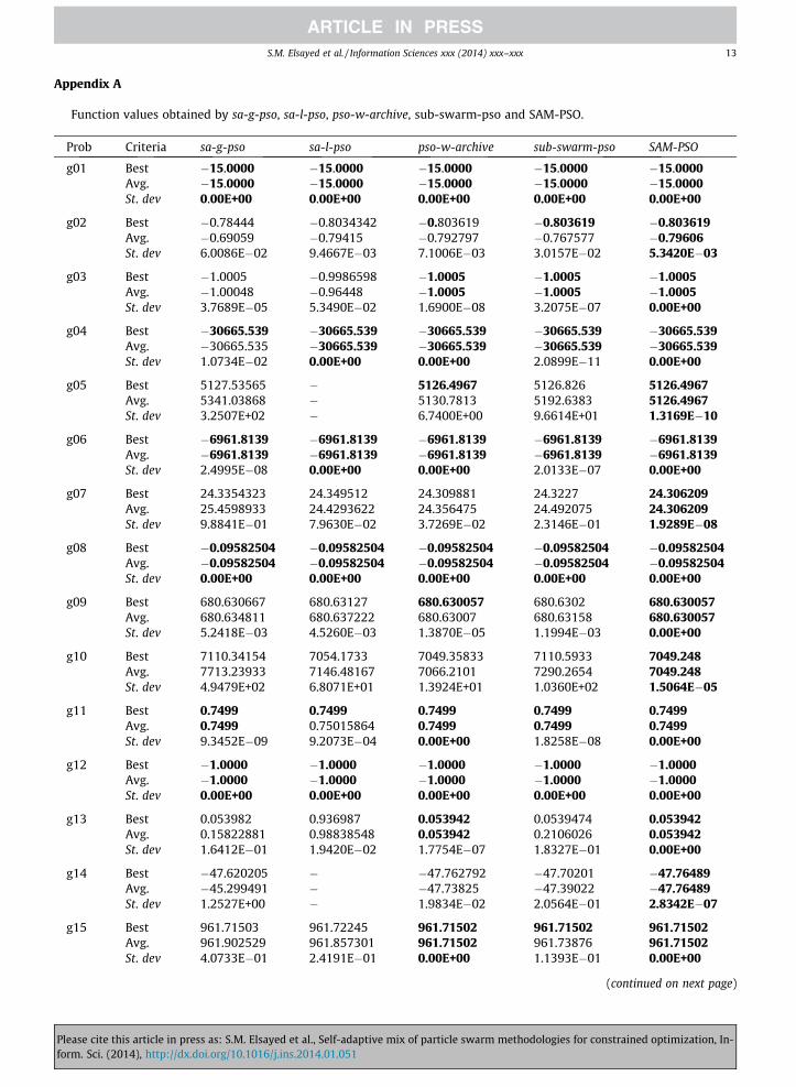
Appendix A
Function values obtained by sa-g-pso, sa-l-pso, pso-w-archive, sub-swarm-pso and SAM-PSO.
Plfo
Prob
ease cite thrm. Sci. (20
Criteria
is article in pres14), http://dx.d
sa-g-pso
s as: S.M. Elsayed et aoi.org/10.1016/j.ins.20
sa-l-pso
l., Self-adaptive mix of14.01.051
pso-w-archive
particle swarm method
sub-swarm-pso
ologies for constrained
SAM-PSO
g01
Best �15.0000 �15.0000 �15.0000 �15.0000 �15.0000 Avg. �15.0000 �15.0000 �15.0000 �15.0000 �15.0000 St. dev 0.00E+00 0.00E+00 0.00E+00 0.00E+00 0.00E+00g02
Best �0.78444 �0.8034342 �0.803619 �0.803619 �0.803619 Avg. �0.69059 �0.79415 �0.792797 �0.767577 �0.79606 St. dev 6.0086E�02 9.4667E�03 7.1006E�03 3.0157E�02 5.3420E�03g03
Best �1.0005 �0.9986598 �1.0005 �1.0005 �1.0005 Avg. �1.00048 �0.96448 �1.0005 �1.0005 �1.0005 St. dev 3.7689E�05 5.3490E�02 1.6900E�08 3.2075E�07 0.00E+00g04
Best �30665.539 �30665.539 �30665.539 �30665.539 �30665.539 Avg. �30665.535 �30665.539 �30665.539 �30665.539 �30665.539 St. dev 1.0734E�02 0.00E+00 0.00E+00 2.0899E�11 0.00E+00g05
Best 5127.53565 � 5126.4967 5126.826 5126.4967 Avg. 5341.03868 � 5130.7813 5192.6383 5126.4967 St. dev 3.2507E+02 � 6.7400E+00 9.6614E+01 1.3169E�10g06
Best �6961.8139 �6961.8139 �6961.8139 �6961.8139 �6961.8139 Avg. �6961.8139 �6961.8139 �6961.8139 �6961.8139 �6961.8139 St. dev 2.4995E�08 0.00E+00 0.00E+00 2.0133E�07 0.00E+00g07
Best 24.3354323 24.349512 24.309881 24.3227 24.306209 Avg. 25.4598933 24.4293622 24.356475 24.492075 24.306209 St. dev 9.8841E�01 7.9630E�02 3.7269E�02 2.3146E�01 1.9289E�08g08
Best �0.09582504 �0.09582504 �0.09582504 �0.09582504 �0.09582504 Avg. �0.09582504 �0.09582504 �0.09582504 �0.09582504 �0.09582504 St. dev 0.00E+00 0.00E+00 0.00E+00 0.00E+00 0.00E+00g09
Best 680.630667 680.63127 680.630057 680.6302 680.630057 Avg. 680.634811 680.637222 680.63007 680.63158 680.630057 St. dev 5.2418E�03 4.5260E�03 1.3870E�05 1.1994E�03 0.00E+00g10
Best 7110.34154 7054.1733 7049.35833 7110.5933 7049.248 Avg. 7713.23933 7146.48167 7066.2101 7290.2654 7049.248 St. dev 4.9479E+02 6.8071E+01 1.3924E+01 1.0360E+02 1.5064E�05g11
Best 0.7499 0.7499 0.7499 0.7499 0.7499 Avg. 0.7499 0.75015864 0.7499 0.7499 0.7499 St. dev 9.3452E�09 9.2073E�04 0.00E+00 1.8258E�08 0.00E+00g12
Best �1.0000 �1.0000 �1.0000 �1.0000 �1.0000 Avg. �1.0000 �1.0000 �1.0000 �1.0000 �1.0000 St. dev 0.00E+00 0.00E+00 0.00E+00 0.00E+00 0.00E+00g13
Best 0.053982 0.936987 0.053942 0.0539474 0.053942 Avg. 0.15822881 0.98838548 0.053942 0.2106026 0.053942 St. dev 1.6412E�01 1.9420E�02 1.7754E�07 1.8327E�01 0.00E+00g14
Best �47.620205 � �47.762792 �47.70201 �47.76489 Avg. �45.299491 � �47.73825 �47.39022 �47.76489 St. dev 1.2527E+00 � 1.9834E�02 2.0564E�01 2.8342E�07g15
Best 961.71503 961.72245 961.71502 961.71502 961.71502 Avg. 961.902529 961.857301 961.71502 961.73876 961.71502 St. dev 4.0733E�01 2.4191E�01 0.00E+00 1.1393E�01 0.00E+00(continued on next page)
optimization, In-

14 S.M. Elsayed et al. / Information Sciences xxx (2014) xxx–xxx
Pfo
g16
lease cite thrm. Sci. (20
Best
is article in pres14), http://dx.d
�1.9051553
s as: S.M. Elsayed et aoi.org/10.1016/j.ins.20
�1.9051553
l., Self-adaptive mix o14.01.051
�1.9051553
f particle swarm method
�1.9051553
ologies for constrained
�1.9051553
Avg. �1.9051553 �1.9051553 �1.9051553 �1.9051553 �1.9051553 St. dev 8.2568E�10 0.00E+00 0.00E+00 0.00E+00 0.00E+00g17
Best 8856.09207 8996.4176 8853.5397 8892.5674 8853.5397 Avg. 9021.31626 9011.12197 8903.4781 8958.4176 8853.5397 St. dev 1.4609E+02 2.0795E+01 3.9396E+01 6.8207E+01 2.1125E�07g18
Best �0.86602 �0.8660079 �0.866025 �0.866025 �0.866025 Avg. �0.8637285 �0.8629285 �0.865853 �0.865186 �0.866025 St. dev 2.6114E�03 4.4663E�03 2.2208E�04 1.2654E�03 7.5801E�08g19
Best 40.9841944 34.166736 32.6954216 33.414259 32.656734 Avg. 68.0547587 36.1279533 33.331036 37.021167 32.66553 St. dev 1.2838E+01 1.3251E+00 5.6921E�01 3.0795E+00 9.8422E�03g20
Best – – – – – Avg. – – – – – St. dev – – – – –g21
Best – – 193.74716 – 32.656235 Avg. – – 193.75381 – 32.666236 St. dev – – 1.8409E–03 – 1.5762E–02g22
Best – – – – – Avg. – – – – – St. dev – – – – –g23
Best �221.88355 – �239.4370012 �122.3332 �400.0551 Avg. 141.657785 – �44.42996588 �19.72075 �400.0512 St. dev 2.1318E+02 – 8.2282E+01 8.3234E+01 1.2014E�03g24 Best �5.508013 �5.508013 �5.508013 �5.508013 �5.508013
Avg. �5.508013 �5.508013 �5.508013 �5.508013 �5.508013 St. dev 0.00E+00 0.00E+00 0.00E+00 0.00E+00 0.00E+00The boldface value means that it is better than that of the other algorithm(s).
Appendix B
Function values obtained by SAM-PSO, CPSO-shake, IPS, SAMO-GA, SAMO-DE, APF-GA and ECHT-EP2 for 24 test problems(in CPSO-shake, ‘�’ and ‘⁄’ symbols mean value not available or infeasible, respectively).
Prob.
Criteria SAM-PSO CPSO-shake IPSO SAMO-GA SAMO-DEo
ECHT-EP2
g01
Best �15.0000 �15 �15.0000 �15.0000 �15.0000 �15.0000 Avg. �15.0000 �15 �15.0000 �15.0000 �15.0000 �15.0000 St. dev 0.00E+00 – 0.00E+00 0.00E+00 0.00E+00 0.00E+00g02 Best �0.803619 �0.803 �0.802629 �0.80359052 �0.8036191 �0.8036191
Avg. �0.79606 �0.79661 �0.713879 �0.79604769 �0.79873521 �0.7998220 St. dev 5.3420E�03 – 4.62 E�02 5.8025E�03 8.8005E�03 1.26E�02g03 Best �1.0005 �1 �0.641 �1.0005 �1.0005 �1.0005
Avg. �1.0005 �1 �0.154 �1.0005 �1.0005 �1.0005 St. dev 0.00E+00 – 1.70 E�01 0.00E+00 0.00E+00 0.00E+00g04 Best �30665.539 �30665.538 �30665.539 �30665.5386 �30665.5386 �30665.539
Avg. �30665.539 �30646.179 �30665.539 �30665.5386 �30665.5386 �30665.539 St. dev 0.00E+00 – 7.40E�12 0.00E+00 0.00E+00 0.00E+00ptimization, In-

S.M. Elsayed et al. / Information Sciences xxx (2014) xxx–xxx 15
Plfo
g05
ease cite trm. Sci. (2
Best
his article in014), http://
5126.4967
press as: S.M. Elsaydx.doi.org/10.1016/
5126.498
ed et al., Self-adapj.ins.2014.01.051
5126.498
tive mix of particle
5126.497
swarm methodolo
5126.497
gies for constrained o
5126.497
Avg. 5126.4967 5240.49671 5135.521 5127.97643 5126.497 5126.497 St. dev 1.3169E�10 � 1.23E+01 1.1166E+00 0.00E+00 0.00E+00g06
Best �6961.8139 �6961.825 �6961.814 �6961.814 �6961.814 �6961.814 Avg. �6961.8139 �6859.0759 �6961.814 �6961.814 �6961.814 �6961.814 St. dev 0.00E+00 – 2.81E�05 0.00E+00 0.00E+00 0.00E+00g07
Best 24.306209 24.309 24.366 24.3062 24.3062 24.3062 Avg. 24.306209 24.9122091 24.691 24.4113 24.3096 24.3063 St. dev 1.9289E�08 – 2.20E�01 4.5905E�02 1.5888E�03 3.19E�05g08
Best �0.09582504 �0.095 �0.095825 �0.09582504 �0.09582504 �0.095825 Avg. �0.09582504 �0.095 �0.095825 �0.09582504 �0.09582504 �0.095825 St. dev 0.00E+00 – 4.23E�17 0.00E+00 0.00E+00 2.61E�08g09
Best 680.630057 680.63 680.638 680.630 680.630 680.630 Avg. 680.630057 681.373057 680.674 680.634 680.630 680.630 St. dev 0.00E+00 – 3.00E�02 1.4573E�03 1.1567E�05 0.00E+00g10
Best 7049.248 7049.285 7053.963 7049.2481 7049.2481 7049.2483 Avg. 7049.248 7850.40102 7306.466 7144.40311 7059.81345 7049.2490 St. dev 1.5064E�05 – 2.22E+02 6.7860E+01 7.856E+00 6.60E�04g11
Best 0.7499 0.7499 0.7499 0.7499 0.7499 0.7499 Avg. 0.7499 0.7499 0.753 0.7499 0.7499 0.7499 St. dev 0.00E+00 – 6.53E�03 0.00E+00 0.00E+00 0.00E+00g12
Best �1.0000 �1 �1.0000 �1.0000 �1.0000 �1.0000 Avg. �1.0000 �1 �1.0000 �1.0000 �1.0000 �1.0000 St. dev 0.00E+00 – 0.00E+00 0.00E+00 0.00E+00 0.00E+00g13 Best 0.053942 0.054 0.066845 0.053942 0.053942 0.053942
Avg. 0.053942 0.45094151 0.430408 0.054028 0.053942 0.053942 St. dev 0.00E+00 – 2.30E+00 5.9414E�05 1.7541E�08 1.00E�12g14 Best �47.76489 �47.635 �47.449 �47.1883 �47.76489 �47.7649
Avg. �47.76489 �45.665888 �44.572 �46.4731793 �47.68115 �47.7648 St. dev 2.8342E�07 – 1.58E+00 3.1590E�01 4.043E�02 2.72E�05g15 Best 961.71502 961.715 961.715 961.71502 961.71502 961.71502
Avg. 961.71502 962.516022 962.242 961.715087 961.71502 961.71502 St. dev 0.00E+00 – 6.20E�01 5.5236E�05 0.00E+00 2.01E�13g16 Best �1.9051553 �1.905 �1.9052 �1.905155 �1.905155 �1.905155
Avg. �1.9051553 �1.7951553 �1.9052 �1.905154 �1.905155 �1.905155 St. dev 0.00E+00 – 2.42E�12 6.9520E�07 0.00E+00 1.12E�10g17 Best 8853.5397 8853.5397 8863.293 8853.5397 8853.5397 8853.5397
Avg. 8853.5397 8894.70867 8911.738 8853.8871 8853.5397 8853.5397 St. dev 2.1125E�07 � 2.73E+01 1.7399E�01 1.1500E�05 2.13E�08g18 Best �0.866025 �0.866 �0.865994 �0.866025 �0.866025 �0.866025
Avg. �0.866025 �0.7870254 �0.862842 �0.865545 �0.866024 �0.866025 St. dev 7.5801E�08 – 4.41E�03 4.0800E�04 7.043672E�07 1.00E�09g19 Best 32.656235 34.018 33.967 32.655592 32.655592 32.6591
Avg. 32.666236 64.505593 37.927 36.427463 32.757340 32.6623 St. dev 1.5762E�02 – 3.20E+00 1.0372E+00 6.145E�02 3.4E�03g20 Best – – – – – –
Avg. – – – – – – St. dev – – – – – –(continued on next page)
ptimization, In-
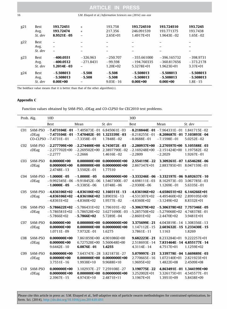
16 S.M. Elsayed et al. / Information Sciences xxx (2014) xxx–xxx
Pfo
g21
lease cite trm. Sci. (2
Best
his article in014), http://
193.72451
press as: S.M. Elsaydx.doi.org/10.1016/
⁄
ed et al., Self-adapj.ins.2014.01.051
193.758
tive mix of particl
193.724510
e swarm methodolo
193.724510
gies for constrained o
193.7245
Avg. 193.72474 ⁄ 217.356 246.091539 193.771375 193.7438 St. dev 8.9521E�05 – 2.65E+01 1.4917E+01 1.9643E�02 1.65E�02g22
Best – – – – – – Avg. – – – – – – St. dev – – – – – –g23
Best �400.0551 �326.963 �250.707 �355.661000 �396.165732 �398.9731 Avg. �400.0512 �271.8431 �99.598 �194.760335 �360.817656 �373.2178 St. dev 1.2014E�03 – 1.20E+02 5.3278E+01 1.9623E+01 3.37E+01g24
Best �5.508013 �5.508 �5.508 �5.508013 �5.508013 �5.508013 Avg. �5.508013 �5.508 �5.508 �5.508013 �5.508013 �5.508013 St. dev 0.00E+00 – 9.03E�16 0.00E+00 0.00E+00 1.8E�15The boldface value means that it is better than that of the other algorithm(s).
Appendix C
Function values obtained by SAM-PSO, eDEag and CO-CLPSO for CEC2010 test problems.
Prob. A
lg. 1 0D 3 0DBest
Mean St. dev B est Mean St. devC01 S
AM-PSO � 7.473104E�01 �7.405873E�01 6.845061E�03 � 8.218844E�01 �7.964331E�01 1.841715E�02 eDEag � 7.473104E�01 �7.470402E�01 1.323339E�03 � 8.218255E�01 �8.208687E�01 7.103893E�04 CO-CLPSO � 7.4731E�01 �7.3358E�01 1.7848E�02 � 8.0688E�01 �7.1598E�01 5.0252E�02C02 S
AM-PSO � 2.277709E+00 �2.274400E+00 6.743072E�03 � 2.280937E+00 �2.270597E+00 5.105588E�03 eDEag � 2.277702E+00 �2.269502E+00 2.3897790E�02 � 2.169248E+00 �2.151424E+00 1.197582E�02�
2.2777 �2.2666 1.4616E�02 � 2.2809 �2.2029 1.9267E�01C03 S
AM-PSO 0.00000E+00 0.000000E+00 0.0000000E+00 2.554119E�22 3.309261E�07 1.654628E�06 eDEag 0.000000E+00 0.000000E+00 0.0000000E+00 2.867347E+01 2.883785E+01 8.047159E�012.4748E�13
3.5502E�01 1.77510 – – –C04 S
AM-PSO � 1.0000E�05 �1.0000E�05 0.0000000E+00 � 3.333246E�06 �3.332197E�06 9.692637E�10 eDEag � 9.992345E�06 �9.918452E�06 1.5467300E�07 4.698111E�03 8.162973E�03 3.067785E�03�
1.0000E�05 �9.3385E�06 1.0748E�06 � 2.9300E�06 1.1269E�01 5.6335E�01C05 S
AM-PSO � 4.836106E+02 �4.836106E+02 1.160311E�13 � 4.836106E+02 �4.658651E+02 6.144266E+01 eDEag � 4.836106E+02 �4.836106E+02 3.89035E�13 � 4.531307E+02 �4.495460E+02 2.899105E+00�
4.8361E+02 �4.8360E+02 1.9577E�02 � 4.8360E+02 �3.1249E+02 8.8332E+01C06 S
AM-PSO � 5.786622E+02 �5.786431E+02 1.796101E�02 � 5.306379E+02 �5.306378E+02 7.757346E�05 eDEag � 5.786581E+02 �5.786528E+02 3.6271690E�03 � 5.285750E+02 �5.279068E+02 4.748378E�01�
5.7866E+02 �5.7866E+02 5.7289E�04 � 2.8601E+02 �2.4470E+02 3.9481E+01C07 S
AM-PSO 0.00000E+00 0.000000E+00 0.0000000E+00 3.375699E�21 4.043819E�14 1.308356E�13 eDEag 0.00000E+00 0.000000E+00 0.0000000E+00 1.147112E�15 2.603632E�15 1.233430E�151.0711E�09
7.9732E�01 1.6275 3.7861E�11 1.1163 1.8269C08 S
AM-PSO 0.000000E+00 7.861859E+00 4.901086E+00 9.682223E�21 8.233284E+01 9.222257E+01 eDEag 0.00000E+00 6.727528E+00 5.560648E+00 2.518693E�14 7.831464E�14 4.855177E�149.6442E�10
6.0876E�01 1.4255 4.3114E�14 4.7517E+01 1.1259E+02C09 S
AM-PSO 0.000000E+00 7.643747E�28 3.821873E�27 5.079997E�21 3.339778E�04 1.669889E�03 eDEag 0.00000E+00 0.000000E+00 0.0000000E+00 2.770665E�16 1.072140E+01 2.821923E+013.7551E�16
1.9938E+10 9.9688E+10 1.9695E+02 1.4822E+08 2.4509E+08C10 S
AM-PSO 0.000000E+00 3.102937E�27 7.259108E�27 3.190775E�22 4.863491E�01 1.344199E+00 eDEag 0.000000E+00 0.000000E+00 0.0000000E+00 3.252002E+01 3.326175E+01 4.545577E�012.3967E�15
4.9743E+10 2.4871E+11 3.1967E+01 1.3951E+09 5.8438E+09ptimization, In-

S.M. Elsayed et al. / Information Sciences xxx (2014) xxx–xxx 17
Plfo
Appendix C (continued)
Prob.
ease crm. Sc
Alg.
ite this articli. (2014), ht
10D
e in press as: S.M. Elsayed et al., Self-adaptive mix of partitp://dx.doi.org/10.1016/j.ins.2014.01.051
30D
Best
Mean S t. dev Bestcle swarm methodo
Mean S
logies for constrain
t. dev
C11
SAM-PSO �1.522713E�03 �1.522713E�03 4.456278E�12 �3.923439E�04 �3.923423E�04 1.362166E�09 eDEag �1.52271E�03 �1.52271E�03 6.3410350E�11 �3.268462E�04 �2.863882E�04 2.707605E�05�
� � � � �C12
SAM-PSO �1.992458E�01 �1.992457E�01 1.193491E�08 �1.992633E�01 �1.992628E�01 3.413745E�07 eDEag �5.700899E+02 �3.367349E+02 1.7821660E+02 �1.991453E�01 3.562330E+02 2.889253E+02�1.2639E+01
�2.3369 2.4329E+01 �1.9926E�01 �1.9911E�01 1.1840E�04C13
SAM-PSO �6.842937E+01 �6.431966E+01 1.974159E+00 �6.358851E+01 �6.143381E+01 1.107755E+00 eDEag �6.842937E+01 �6.842936E+01 1.0259600E�06 �6.642473E+01 �6.535310E+01 5.733005E�01�6.842936E+01
�6.397445E+01 2.134080E+00 �6.2752E+01 �6.0774E+01 1.1176C14
SAM-PSO 0.000000E+00 0.000000E+00 0.0000000E+00 1.227861E�20 6.080968E�13 2.804565E�12 eDEag 0.000000E+00 0.000000E+00 0.0000000E+00 5.015863E�14 3.089407E�13 5.608409E�135.7800E�12
3.1893E�01 1.1038 3.28834e�09 0.0615242 0.307356C15
SAM-PSO 0.000000E+00 0.000000E+00 0.0000000E+00 4.642754E�23 3.767962E�06 1.883981E�05 eDEag 0.000000E+00 1.798980E�01 8.8131560E�01 2.160345E+01 2.160376E+01 1.104834E�043.0469E�12
2.9885 3.3147 5.7499E�12 5.1059E+01 9.1759E+01C16
SAM-PSO 0.000000E+00 0.000000E+00 0.000000E+00 0.000000E+00 0.000000E+00 0.000000E+00 eDEag 0.000000E+00 3.702054E�01 3.7104790E�01 0.000000E+00 2.168404E�21 1.062297E�200.000000E+00
5.9861E�03 1.3315E�02 0.000000E+00 5.2403E�16 4.6722E�16C17
SAM-PSO 0.000000E+00 2.711709E�33 3.122304E�33 1.089699E�08 5.433162E�02 8.983999E�02 eDEag 1.463180E�17 1.249561E�01 1.9371970E�01 2.165719E�01 6.326487E+00 4.986691E+007.6677E�17
3.7986E�01 4.5284E�01 1.5787E�01 1.3919 4.2621C18
SAM-PSO 0.000000E+00 2.287769E�22 1.075245E�21 2.398722E�10 4.828803E�06 1.399493E�05 eDEag 3.731440E�20 9.678765E�19 1.8112340E�18 1.226054E+00 8.754569E+01 1.664753E+027.7804E�21
2.3192E�01 9.9559E�01 6.0047E�02 1.0877E+01 3.7161E+01The boldface value means that it is better than that of the other algorithm(s).
References
[1] M.A. Abido, Optimal design of power-system stabilizers using particle swarm optimization, IEEE Trans. Energy Convers. 17 (2002) 406–413.[2] L. Cagnina, S. Esquivel, C.A. Coello Coello, A particle swarm optimizer for constrained numerical optimization, in: T. Runarsson, H.-G. Beyer, E. Burke, J.
Merelo-Guervós, L. Whitley, X. Yao (Eds.), Parallel Problem Solving from Nature – PPSN IX, Springer, Berlin/Heidelberg, 2006, pp. 910–919.[3] L.C. Cagnina, S.C. Esquivel, C.A. Coello Coello, Solving constrained optimization problems with a hybrid particle swarm optimization algorithm, Eng.
Optim. 43 (2011) 843–866.[4] W.N. Chen, J. Zhang, Y. Lin, N. Chen, Z.H. Zhan, H.S.H. Chung, Y. Li, Y.H. Shi, Particle swarm optimization with an aging leader and challengers, IEEE
Trans. Evol. Comput. 17 (2013) 241–258.[5] J. Chia-Feng, C. Yu-Cheng, Evolutionary-group-based particle-swarm-optimized fuzzy controller with application to mobile-robot navigation in
unknown environments, IEEE Trans. Fuzzy Syst. 19 (2011) 379–392.[6] M. Clerc, J. Kennedy, The particle swarm – explosion, stability, and convergence in a multidimensional complex space, IEEE Trans. Evol. Comput. 6
(2002) 58–73.[7] G.W. Corder, D.I. Foreman, Nonparametric Statistics for Non-Statisticians: A Step-by-Step Approach, John Wiley, Hoboken, NJ, 2009.[8] K. Deb, An efficient constraint handling method for genetic algorithms, Comput. Methods Appl. Mech. Eng. 186 (2000) 311–338.[9] Y. del Valle, G.K. Venayagamoorthy, S. Mohagheghi, J.C. Hernandez, R.G. Harley, Particle swarm optimization: basic concepts, variants and applications
in power systems, IEEE Trans. Evol. Comput. 12 (2008) 171–195.[10] A.E. Eiben, I.G. Sprinkhuizen-Kuyper, B.A. Thijssen, Competing crossovers in an adaptive GA framework, in: IEEE Congress on Evolutionary
Computation, IEEE, 1998, pp. 787–792.[11] S. Elsayed, R. Sarker, D. Essam, Memetic multi-topology particle swarm optimizer for constrained optimization, in: IEEE Congress on Evolutionary
Computation, World Congress on Computational Intelligence (WCCI2012), IEEE, Brisbane, 2012.[12] S. Elsayed, R. Sarker, D. Essam, Self-adaptive differential evolution incorporating a heuristic mixing of operators, Comput. Optim. Appl. (2012) 1–20.[13] S. Elsayed, R. Sarker, T. Ray, Parameters adaptation in differential evolution, in: IEEE Congress on Evolutionary Computation, Brisbane, IEEE, 2012, pp.
1–8.[14] S.M. Elsayed, R.A. Sarker, D.L. Essam, An improved self-adaptive differential evolution algorithm for optimization problems, IEEE Trans. Indust. Inform.
9 (2013) 89–99.[15] S.M. Elsayed, R.A. Sarker, D.L. Essam, Multi-operator based evolutionary algorithms for solving constrained optimization problems, Comput. Oper. Res.
38 (2011) 1877–1896.[16] S.M. Elsayed, R.A. Sarker, D.L. Essam, On an evolutionary approach for constrained optimization problem solving, Appl. Soft Comput. 12 (2012) 3208–
3227.
ed optimization, In-

18 S.M. Elsayed et al. / Information Sciences xxx (2014) xxx–xxx
[17] A. Engelbrecht, Heterogeneous particle swarm optimization, in: M. Dorigo, M. Birattari, G. Di Caro, R. Doursat, A. Engelbrecht, D. Floreano, L.Gambardella, R. Groß, E. Sahin, H. Sayama, T. Stützle (Eds.), Swarm Intelligence, Springer, Berlin/Heidelberg, 2010, pp. 191–202.
[18] A.P. Engelbrecht, Scalability of a heterogeneous particle swarm optimizer, in: 2011 IEEE Symposium on Swarm Intelligence (SIS), IEEE, 2011, pp. 1–8.[19] D. Goldberg, Genetic Algorithms in Search, Optimization, and Machine Learning, Addison-Wesley, MA, 1989.[20] Q. He, L. Wang, An effective co-evolutionary particle swarm optimization for constrained engineering design problems, Eng. Appl. Artif. Intell. 20
(2007) 89–99.[21] S. He, E. Prempain, Q.H. Wu, An improved particle swarm optimizer for mechanical design optimization problems, Eng. Optim. 36 (2004) 585–605.[22] Hu, X., R. Eberhart, Solving constrained nonlinear optimization problems with particle swarm optimization, in: the 6th World Multiconference on
Systemics, Cybernetics and Informatics, 2002, pp. 203–206.[23] Y. Hyun-Sook, M. Byung-Ro, An empirical study on the synergy of multiple crossover operators, IEEE Trans. Evol. Comput. 6 (2002) 212–223.[24] Y.-T. Juang, S.-L. Tung, H.-C. Chiu, Adaptive fuzzy particle swarm optimization for global optimization of multimodal functions, Inform. Sci. 181 (2011)
4539–4549.[25] J. Kennedy, R. Eberhart, Particle swarm optimization, in: IEEE International Conference on Neural Networks, IEEE, 1995, pp. 1942–1948.[26] B.J. Leonard, A.P. Engelbrecht, A.B. van Wyk, Heterogeneous particle swarms in dynamic environments, in: IEEE Symposium on Swarm Intelligence
(SIS), IEEE, 2011, pp. 1–8.[27] J.J. Liang, T.P. Runarsson, E. Mezura-Montes, M. Clerc, P.N. Suganthan, C.A. Coello Coello, K. Deb, Problem Definitions and Evaluation Criteria for the CEC
2006 Special Session on Constrained Real-Parameter Optimization, Technical Report, Nanyang Technological University, Singapore, 2005.[28] J.J. Liang, Z. Shang, Z. Li, Coevolutionary comprehensive learning particle swarm optimizer, in: IEEE Congress on Evolutionary Computation, IEEE, 2010,
pp. 1–8.[29] J.J. Liang, P.N. Suganthan, Dynamic multi-swarm particle swarm optimizer with a novel constraint-handling mechanism, in: IEEE Congress on
Evolutionary Computation, IEEE, 2006, pp. 9–16.[30] R. Mallipeddi, S. Mallipeddi, P.N. Suganthan, M.F. Tasgetiren, Differential evolution algorithm with ensemble of parameters and mutation strategies,
Appl. Soft Comput. 11 (2011) 1679–1696.[31] R. Mallipeddi, P.N. Suganthan, Differential evolution with ensemble of constraint handling techniques for solving CEC 2010 benchmark problems, in:
IEEE Congress on Evolutionary Computation, IEEE, 2010, pp. 1–8.[32] R. Mallipeddi, P.N. Suganthan, Ensemble of constraint handling techniques, IEEE Trans. Evol. Comput. 14 (2010) 561–579.[33] R. Mallipeddi, P.N. Suganthan, Problem Definitions and Evaluation Criteria for the CEC 2010 Competition and Special Session on Single Objective
Constrained Real-parameter Optimization, Technical Report, Nangyang Technological University, Singapore, 2010.[34] R. Mendes, J. Kennedy, J. Neves, The fully informed particle swarm: simpler, maybe better, IEEE Trans. Evol. Comput. 8 (2004) 204–210.[35] E. Mezura-Montes, J. Flores-Mendoza, Improved particle swarm optimization in constrained numerical search spaces, in: R. Chiong (Ed.), Nature-
Inspired Algorithms for Optimisation, Springer, Berlin/Heidelberg, 2009, pp. 299–332.[36] M.A. Montes de Oca, J. Pena, T. Stutzle, C. Pinciroli, M. Dorigo, Heterogeneous particle swarm optimizers, in: IEEE Congress on Evolutionary
Computation, IEEE, 2009, pp. 698–705.[37] F. Nepomuceno, A. Engelbrecht, A self-adaptive heterogeneous PSO inspired by ants, in: M. Dorigo, M. Birattari, C. Blum, A. Christensen, A.
Engelbrecht, R. Groß, T. Stützle (Eds.), Swarm Intelligence, Springer, Berlin Heidelberg, 2012, pp. 188–195.[38] F. Neri, E. Mininno, G. Iacca, Compact particle swarm optimization, Inform. Sci. 239 (2013) 96–121.[39] O. Olorunda, A.P. Engelbrecht, An analysis of heterogeneous cooperative algorithms, in: IEEE Congress on Evolutionary Computation, IEEE, 2009, pp.
1562–1569.[40] M. Omran, A.P. Engelbrecht, A. Salman, Particle swarm optimization method for image clustering, Int. J. Pattern Recognit. Artif. Intell. 19 (2005) 297–321.[41] K. Parsopoulos, M. Vrahatis, Unified particle swarm optimization for solving constrained engineering optimization problems, in: L. Wang, K. Chen, Y.
Ong (Eds.), Advances in Natural Computation, Springer, Berlin/Heidelberg, 2005, pp. 582–591.[42] K. Parsopoulos, M. Vrahatis, Unified particle swarm optimization for solving constrained engineering optimization problems, in: L. Wang, K. Chen, Y.
Ong (Eds.), Advances in Natural Computation, Springer, Berlin/Heidelberg, 2005, pp. 582–591.[43] Y.V. Pehlivanoglu, A new particle swarm optimization method enhanced with a periodic mutation strategy and neural networks, IEEE Trans. Evol.
Comput. 17 (2013) 436–452.[44] G.T. Pulido, C.A. Coello Coello, A constraint-handling mechanism for particle swarm optimization, in: IEEE Congress on Evolutionary Computation,
IEEE, 2004, pp. 1396–1403.[45] A.K. Qin, V.L. Huang, P.N. Suganthan, Differential evolution algorithm with strategy adaptation for global numerical optimization, IEEE Trans. Evol.
Comput. 13 (2009) 398–417.[46] B.Y. Qu, P.N. Suganthan, S. Das, A distance-based locally informed particle swarm model for multimodal optimization, IEEE Trans. Evol. Comput. 17
(2013) 387–402.[47] T. Ray, K.M. Liew, A swarm with an effective information sharing mechanism for unconstrained and constrained single objective optimisation
problems, in: IEEE Congress on Evolutionary Computation, IEEE, 2001, pp. 75–80.[48] A.K. Renato, C. Leandro dos Santos, Coevolutionary particle swarm optimization using Gaussian distribution for solving constrained optimization
problems, IEEE Trans. Syst. Man Cybernet. Part B: Cybernet. 36 (2006) 1407–1416.[49] Y. Shi, H. Liu, L. Gao, G. Zhang, Cellular particle swarm optimization, Inform. Sci. 181 (2011) 4460–4493.[50] P. Spanevello, M.A.M.d. Oca, Experiments on adaptive heterogeneous PSO algorithms, in: Doctoral Symposium on Engineering Stochastic Local Search
Algorithms, IRIDIA, Institut de Re her hes Interdisiplinaires, Université Libre de Bruxelles, Belgium, 2009, pp. 36–40.[51] W.M. Spears, Adapting crossover in evolutionary algorithms, in: J.R. McDonnell, R.G. Reynolds, D.B. Fogel (Eds.), The 4th Annual Conference on
Evolutionary Programming, MIT Press, 1995, pp. 367–384.[52] R. Storn, K. Price, Differential evolution – a simple and efficient adaptive scheme for global optimization over continuous spaces, in: Technical Report,
International Computer Science Institute, 1995.[53] L. Sun, S. Yoshida, X. Cheng, Y. Liang, A cooperative particle swarm optimizer with statistical variable interdependence learning, Inform. Sci. 186 (2012)
20–39.[54] T. Takahama, S. Sakai, Constrained optimization by the e constrained differential evolution with an archive and gradient-based mutation, in: IEEE
Congress on Evolutionary Computation, IEEE, 2010, pp. 1–9.[55] M.F. Tasgetiren, P.N. Suganthan, P. Quan-Ke, R. Mallipeddi, S. Sarman, An ensemble of differential evolution algorithms for constrained function
optimization, in: IEEE Congress on Evolutionary Computation, IEEE, 2010, pp. 1–8.[56] H. Wang, I. Moon, S. Yang, D. Wang, A memetic particle swarm optimization algorithm for multimodal optimization problems, Inform. Sci. 197 (2012)
38–52.[57] H. Wang, H. Sun, C. Li, S. Rahnamayan, J.-S. Pan, Diversity enhanced particle swarm optimization with neighborhood search, Inform. Sci. 223 (2013)
119–135.[58] Y. Wang, B. Li, T. Weise, J. Wang, B. Yuan, Q. Tian, Self-adaptive learning based particle swarm optimization, Inform. Sci. 181 (2011) 4515–4538.[59] T. Xiaoyong, Y. Fei, C. Ruijuan, Path planning of underwater vehicle based on particle swarm optimization, in: 2010 International Conference on
Intelligent Control and Information Processing (ICICIP), 2010, pp. 123–126.[60] E. Zahara, Y.-T. Kao, Hybrid Nelder–Mead simplex search and particle swarm optimization for constrained engineering design problems, Expert Syst.
Appl. 36 (2009) 3880–3886.[61] G. Zwe-Lee, A particle swarm optimization approach for optimum design of PID controller in AVR system, IEEE Trans. Energy Convers. 19 (2004) 384–
391.
Please cite this article in press as: S.M. Elsayed et al., Self-adaptive mix of particle swarm methodologies for constrained optimization, In-form. Sci. (2014), http://dx.doi.org/10.1016/j.ins.2014.01.051


![PREPRINT 1 Visibility Constrained Generative Model for ... · ous correspondences well [11], [14], [15], [43]. Possible reme-dies include particle swarm optimization [44] for optimizing](https://static.fdocuments.us/doc/165x107/5f121d16c394af76c92153ff/preprint-1-visibility-constrained-generative-model-for-ous-correspondences-well.jpg)


