In Proceedings of the International Symposium on Code Generation and Optimization (CGO 2006).

Selecting Software Phase Markers with Code Structure Analysis

Jeremy Lau Erez Perelman Brad Calder

Department of Computer Science and EngineeringUniversity of California, San Diego{jl,eperelma,calder}@cs.ucsd.edu

Abstract

Most programs are repetitive, where similar behavior canbe seen at different execution times. Algorithms have beenproposed that automatically group similar portions of a pro-gram’s execution into phases, where samples of execution inthe same phase have homogeneous behavior and similar re-source requirements. In this paper, we present an automatedprofiling approach to identify code locations whose execu-tions correlate with phase changes. These “software phasemarkers” can be used to easily detect phase changes acrossdifferent inputs to a program without hardware support.

Our approach builds a combined hierarchical procedurecall and loop graph to represent a program’s execution,where each edge also tracks the max, average, and standarddeviation in hierarchical execution variability on paths fromthat edge. We search this annotated call-loop graph for in-structions in the binary that accurately identify the start ofunique stable behaviors across different inputs.

We show that our phase markers can be used to accu-rately partition execution into units of repeating homoge-neous behavior by counting execution cycles and data cachehits. We also compare the use of our software markers toprior work on guiding data cache reconfiguration using data-reuse markers. Finally, we show that the phase markers canbe used to partition the program’s execution at code transi-tions to pick accurately simulation points for SimPoint. Whensimulation points are defined in terms of phase markers, theycan potentially be re-used across inputs, compiler optimiza-tions, and different instruction set architectures for the samesource code.

1 Introduction

The behavior of a program is not random - as programsexecute, they exhibit cyclic behavior patterns. Recent re-search [1, 6, 7, 24, 25, 26, 22, 8], shows that it is possible toaccurately identify and predict these phases in program exe-cution. There are many applications of phase behavior - forexample phases can be exploited to accelerate architecturesimulations [24, 25], to save energy by dynamically recon-figuring caches or processor issue width [1, 26, 7, 6], or toguide compiler optimizations [19, 2].

In prior work [25, 26] we classified a program into phasesby first dividing a program’s execution into non-overlappingfixed-length intervals of 1, 10, or 100 million instructions.An interval is a contiguous portion of execution (a slice intime) of a program. A phase is a set of intervals within aprogram’s execution with similar behavior (e.g., IPC, cache

miss rates, branch miss rates, etc), regardless of temporal ad-jacency. This means that intervals that belong to a phase mayappear throughout the program’s execution. Our prior workuses an off-line clustering algorithm to break a program’sexecution into phases to perform fast and accurate architec-ture simulation by simulating a single representative portionof each phase of execution [25, 16, 26, 22]. We also de-veloped an on-line hardware algorithm to dynamically iden-tify phase behavior to guide adaptive architecture reconfigu-ration [26, 17]. This prior work also relied on fixed lengthintervals of execution.

The goal of this paper is to find phase transitions thatmatch the procedure call and loop structure of programs, in-stead of using fixed length intervals. We select a subset ofeach program’s procedures and loop boundaries to serve asinterval endpoints. Because each interval is aligned with codeboundaries, the program’s execution is divided into VariableLength Intervals (VLIs) of execution. We use the code ateach selected procedure or loop boundary as a software phasemarker that, when executed, signals a phase change withoutany hardware support. These software phase markers are se-lected by analyzing each program’s procedure call and loopiteration patterns.

In this paper we present the formation of a HierarchicalCall-Loop graph, which we use to find the software phasemarkers. The graph contains local and hierarchical executiontime for each procedure call and loop, as well as the varianceon all paths from each call or loop. We present a simple andfast algorithm to select code structures that serve as softwarephase markers from the Call-Loop graph. We show that thesoftware phase markers accurately identify phase changes atthe binary level, with no hardware support, across differentinputs to the program.

The remainder of the paper is laid out as follows. First,prior work in phase analysis is examined in Section 2. Thesimulation framework used in this work is described in Sec-tion 3. Section 4 presents the method for generating the hier-archical call-loop graph, and Section 5 presents the algorithmfor selecting phase markers. Section 6 exams applying thecode phase markers to data cache reconfiguration and Sim-Point. Our findings are summarized in Section 7.

2 Phase Behavior and Related Work

In this section we give a brief overview of recent related workon phase analysis, and provide more detailed descriptions ofthe two areas of research closest related to ours – proceduralphase analysis, distance reuse software phase markers, and

1

using Sequitur to create variable length intervals.

2.1 Related Phase Analysis WorkProgram phase behavior can be detected by examining a pro-gram’s working set [4], and several researchers have recentlyexamined phase behavior in programs.

Balasubramonian et. al. [1] proposed using hardwarecounters to collect miss rates, CPI and branch frequency in-formation for every hundred thousand instructions. They usethe miss rate and the total number of branches executed foreach interval to dynamically evaluate the program’s stability.They used their approach to guide dynamic cache reconfigu-ration to save energy without sacrificing performance.

Dhodapkar and Smith [6, 7, 5] found a relationship be-tween phases and instruction working sets, and that phasechanges occur when the working set changes. They proposeddynamic reconfiguration of multi-configuration units in re-sponse to phase changes indicated by working set changes.They use working set analysis for reconfiguration of in-struction cache, data cache and branch predictor to save en-ergy [6, 7].

Hind et. al. [11] provide a framework for defining andreasoning about program phase classifications, focusing onhow to best define granularity and similarity to perform phaseanalysis.

Sherwood et. al. [24, 25] proposed that periodic phasebehavior in programs can be automatically identified by pro-filing the code executed. We used techniques from machinelearning to classify the execution of the program into phases(clusters). We found that intervals of execution grouped intothe same phase had similar behavior across all architecturalmetrics examined. From this analysis, we created a toolcalled SimPoint [25], which automatically identifies a smallset of intervals of execution (simulation points) in a programfor detailed architectural simulation. These simulation pointsprovide an accurate and efficient representation of the com-plete execution of the program. We then extended this ap-proach to perform hardware phase classification and predic-tion [26, 17]. In [17] we focus on hardware techniques foraccurately classifying and predicting phase changes (transi-tions).

Isci and Martonosi [13, 14] have shown the ability todynamically identify the power phase behavior using powervectors. Deusterwald et. al. [8] recently used hardware coun-ters and other phase prediction architectures to find phase be-havior.

2.2 Basic Block VectorsBasic Block Vectors (BBVs) [24] capture information aboutchanges in a program’s behavior over time. A basic blockis a single-entry, single-exit section of code with no internalcontrol flow. A Basic Block Vector (BBV) is a one dimen-sional array where each element in the array corresponds toone static basic block in the program. We use the BBV struc-ture when using our variable length intervals with SimPoint.We start with a BBV containing all zeroes at the beginningof each interval of execution. During each interval, we countthe number of times each basic block in the program has been

executed, and we record the count in the BBV. For example,if the 50th basic block is executed 15 times in the currentinterval, then bbv[50] = 15. We multiply each count by thenumber of instructions in the basic block, so basic blockscontaining more instructions will have more weight in theBBV.

We used BBVs to compare the intervals of the applica-tion’s execution [24, 25]. The intuition behind this is thatthe behavior of the program at a given time is directly re-lated to the code executed during that interval. Basic blockvectors are fingerprints for each interval of execution: eachvector indicates what portions of code are executed, and howfrequently those portions of code are executed. BBVs areused to evaluate the similarity of their corresponding inter-vals. If the distance between the BBVs is small, then the twointervals spend about the same amount of time in roughly thesame code, and therefore the performance of those two in-tervals should be similar. We compare our software phasemarker approach to basic block vectors, since it is one of themore accurate techniques for phase classification [5].

2.3 Procedure and Loop Phase AnalysisOur approach is based on analyzing an application’s proce-dure and loop structure and variance on execution paths topartition a program’s execution into phases. This approachis motivated by prior work that used fixed length vectors ofloop and procedure counts to identify phase behavior, andprior work [12, 18, 9] into finding phase behavior at the pro-cedure and loop level.

Huang et. al. [12] proposed a hardware algorithm fortracking procedure calls via a call stack, which they used witha set of thresholds to break a program’s execution into phasesat the procedure level. They focus on using a hardware archi-tecture to dynamically find and track these phases. Georgeset. al. [9] implemented their approach to perform offlinephase analysis of Java programs. They implement Huang’salgorithm off-line to provide a workload case study on phasebehavior in Java programs. For both of these works, onlyprocedures are considered for splitting a program’s executioninto phases, and no software marking approach is examined.

In [16], we examined different structures for off-linephase classification, including code signature vectors whereeach dimension represents static procedure calls, returns andloop branches in the binary. These code signatures wereused for phase analysis with fixed length intervals. From thisanalysis, we found that tracking procedures alone resulted inmore intra-phase performance variation compared to trackingboth loops and procedures.

In our work we found that it is important to use loops inaddition to procedures, because loops give us more detailedinformation about the program’s behavior patterns. Also, theutility of procedures for phase classification depends on theprogrammer’s ability to abstract their code into useful andmeaningful subroutines. As an extreme example, procedure-based analysis is very limited if the programmer writes alltheir code in main.

Huang et. al. [18] recently considered procedures andloops to partition a program’s execution. The partitioning de-

2

termined where and when statistical samples should be takenduring architecture simulation. Their analysis broke up a pro-gram’s execution at static call sites, and if a procedure exe-cuted for too long, they divided the procedure’s executioninto its major loops. To determine the sample rate, they ex-amine the variability of several architecture metrics for eachprogram region. Both [16, 18] focused on dividing a pro-gram’s execution trace into intervals of execution based onprocedure calls and loop branches to guide architecture sim-ulation. In comparison, our current work focuses on build-ing a procedure call-loop graph to divide a program’s execu-tion into phases of repeating homogeneous behavior, and weuse this graph to select code constructs that serve as softwarephase markers that indicate phase changes when executed.In addition, we examine an architecture metric independentmethod for modeling variance to determine if a call-loop sitehas too much hierarchical variance when picking softwarephase markers.

2.4 Software Phase MarkingThe closest prior work to ours is the work by Shen et. al. [23],where they use Wavelets [3] and Sequitur [21] to build a hi-erarchy of phase information to represent the program’s be-havior patterns. Their approach is very different from ours,since they perform their phase analysis using data reuse dis-tance and identify phases with advanced analysis techniques(wavelets and Sequitur), while our approach is based ona program’s code structure, represented with our call-loopgraph, which can be analyzed very quickly with a simplegraph algorithm.

Shen et. al. [23] take the data reuse distance phases at thefinest granularity and use Sequitur to find patterns in the datareuse trace, then express each pattern as a regular expression.They then select software phase markers that indicate the be-ginning of each data reuse pattern by finding basic blockswhose execution patterns are highly correlated with the datareuse patterns. Because they select their phase markers withreuse distance, they are able to find phase markers for pro-grams with stable periodic behavior, but they found it diffi-cult to find structure in more complex programs like gcc andvortex. We show that our approach can find phase behav-ior in all programs we examine including gcc and vortex,and we compare our approach to the approach of Shen et.al. [23] for guiding data cache reconfiguration. The goal ofour paper is to (a) run our analysis in a matter of minutes, (b)create phase markers that can be inserted into the binary, and(c) apply our phase analysis to architecture reconfigurationand SimPoint.

3 Methodology and Metrics

For all of the results examined we perform our phase analysison a subset of the SPECINT2000 benchmark suite. We choseprograms that were used in prior phase analysis papers, andthat were shown to be more challenging to perform accuratephase analysis for [15]. In particular, we show results forgcc and vortex since the data phase marker approach ofShen et. al. [23], could not be used to find phase behavior

due to the irregular data behavior in these two programs.The baseline architecture modeled is the same as in prior

work [25]. Each of the SPEC programs were simulated tocompletion to collect the baseline results. We also provideresults for data cache reconfiguration, which were simulatedusing a modified version of the ATOM [27] cache simula-tor used in [23]. For the data cache reconfiguration resultswe compare against the reuse distance-based software phasemarking approach of Shen et. al. in [23]. Shen was very gra-cious to provide us with the exact binaries he used, the reusedistance phase markers he selected, and their ATOM-basedCheetah simulator, which allowed us to do a fair comparisonto their approach. For the comparison, we used the same bi-naries they examined, which consists of tomcatv, swim,compress95, mesh, applu.

3.1 Metrics for Evaluating Phase ClassificationSince phases are intervals with similar program behavior, wemeasure the effectiveness of our phase classifications by ex-amining the similarity of program metrics within each phase.After classifying a program’s intervals into phases, we ex-amine each phase and calculate the average of some metric(CPI, for example) over all intervals in the phase. We thencalculate the standard deviation of the metric for each phase,and we divide the standard deviation by the average to getthe Coefficient of Variation (CoV). CoV measures standarddeviation as a fraction of the average. When we compute theaverage and the standard deviation, we weight each intervalby the number of instructions in the interval, so intervals thatrepresent a larger percentage of the program’s execution re-ceive more weight in the CoV calculations. By averaging theper-phase CoVs across all phases, we have an overall CoVthat measures the homogeneity of a phase classification. Bet-ter phase classifications will exhibit lower overall CoV. If allof the intervals in the same phase have exactly the same CPI,then the overall CoV will be zero.

Unfortunately, CoV is not a perfect metric - if a programwith N intervals is classified into N phases, the CoV will bezero. For this reason, we also examine the number of inter-vals and phases for each classification.

4 Representing Program Behavior with a Proce-dure and Loop Graph

In this section we describe the hierarchical call-loop graphwhich guides the placement of software phase markers. Thecall-loop graph is a call graph extended with nodes for loops,where each node and edge is annotated with hierarchical in-struction counts and standard deviation in hierarchical in-struction count.

4.1 Procedure, Loops, and Phase BehaviorHuang et al [12] found that program behavior tends to befairly homogeneous across different invocations of the sameprocedure. We find that this result extends to loops as well:program behavior across loop iterations and across differentexecutions of the same loop nest are fairly homogeneous.We show this in the next section by showing that the Co-efficient of Variation is not significantly affected by dividing

3

a program’s execution into procedures and loops, comparedto only procedures. Placing phase markers on loops allowsfor smaller interval sizes compared to procedures alone.

While procedures are sufficient for detecting phase be-havior in many programs, like Java applications with smallobject oriented routines [9], we believe that it is also impor-tant to examine a program’s loop structure because proce-dures rely on the programmer to divide their code into mean-ingful subroutines. In prior studies with SimPoint on theSPEC 2000 benchmark suite, we found tracking loops andprocedures to be an effective way to detect phase behavior,while tracking only procedures was not as effective [16].

The call-loop graph has nodes for both procedures andloops. Each node and edge in the call-loop graph carries thecall count, total local and hierarchical dynamic instructioncount, as well as the average and standard deviation of thehierarchical dynamic instruction count.

4.2 Creating a Call-Loop Graph for Finding Phase Be-havior

For our analysis we create a hierarchical call-loop graphwhere edges are annotated with the hierarchical dynamic in-struction counts. We build the call-loop graph by analyz-ing binaries with ATOM [27]. Procedures are detected byATOM, and we identify loop back edges by looking for non-interprocedural backwards branches. A loop is the static coderegion from the backwards branch to its target. There arenodes for both procedures and loops in the call-loop graph.

The call-loop graph tracks the hierarchical instructioncounts for each edge. For a call, this is the total number ofinstructions executed between call and return. For each edgewe keep track of (a) for procedures, the number of times theprocedure is called, and for loops, the number of times theloop iterates, (b) the maximum number of instructions exe-cuted on a single traversal of the edge, (c) the average num-ber of instructions executed on each edge, and (d) the stan-dard deviation in the number of instructions executed on eachedge.

In the call-loop graph, each procedure and loop is rep-resented with two nodes to handle recursion and iteration.Each procedure and loop is represented with a head node anda body node. Every head node always has exactly one child,which is its corresponding body node.

For loops, the loop head node keeps track of how muchtime elapses between loop entry and exit, while the loop bodynode keeps track of how much time elapses in each loop iter-ation. If a loop head is selected as a phase marker, then entryto the loop are marked; if a loop body is selected as a phasemarker, then each loop iteration is marked.

For procedures, the head nodes keep track of elapsed timefor recursive procedures. Procedure body nodes keep trackof statistics for each recursive iteration, similar to the loop-body nodes. For non-recursive procedures, the head and bodynodes carry identical information.

By representing each procedure and loop with head andbody nodes, we can identify more stable program behaviors.For example, we can tell if a loop does similar amounts of

work on each iteration, and we can also tell if a loop doessimilar amounts of work between each entry and exit.

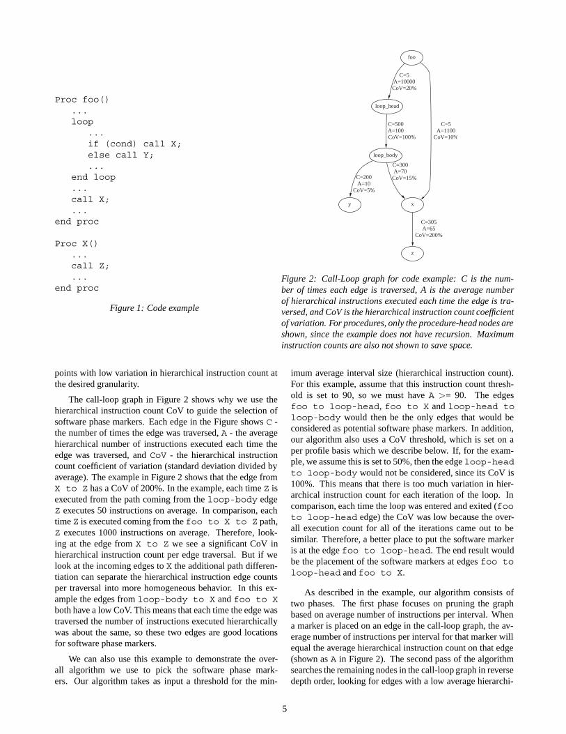
Figure 1 shows an example piece of code and Figure 2shows a simplified call-loop graph corresponding to thiscode. Because there is no recursion in this example, we onlyshow the procedure head nodes in the call-loop graph. Tosave space in the example, the maximum count of instruc-tions is not shown for the edges. Procedure foo contains aloop and the edge between foo and the loop-head con-tains the hierarchical instruction count from loop entry toloop exit. In comparison, the loop-head to loop-bodyedge contains the hierarchical instruction count for each loopiteration. Two nodes are used to represent the loop, and theweight of the edge from foo to loop-head indicates thenumber of times the loop is entered, and the weight of theedge from loop-head to loop-body indicates the num-ber of times the loop iterates.

As shown in Figure 2, each edge in the call-loop graphtracks three values: the number of times the edge was tra-versed (C), the average number of instructions executed eachtime the edge is traversed (A), and the standard deviation ofthe number of instructions across invocations, which is repre-sented in Figure 2 as the Coefficient of Variation (CoV). CoVis just the standard deviation divided by the average. We usethe CoV to find edges with low variance, which become can-didates for phase marker selection, as described in the nextsection.

5 Selecting Software Phase Markers

Software phase markers are points in the binary that can beinstrumented (branches, procedure calls, returns, loop en-tries, the start of a procedure, etc) to reliably indicate thebeginning of a interval of repeating program behavior whenexecuted. These software phase markers can be used to eas-ily and accurately predict program phase changes at run-timewith no hardware support. In addition, software phase mark-ers can be used to predict phase changes across different in-puts to a program, and across different compilations of thesame source code.

In this section, we discuss our software phase marker se-lection algorithm. Given a call-loop graph as described in theprior section, our algorithm selects phase markers that can beinserted into a program with a static or dynamic compiler orbinary instrumentation.

5.1 Selecting Markers from the Call-Loop GraphMany programs exhibit repeating behavior at different timescales. When selecting software phase markers, the selec-tion algorithm needs to know whether the user is interestedin large or small scale behaviors. For example, optimiza-tions with high overheads will be more interested in large-scale phase behavior, since they require more time betweenoptimizations to recoup the cost of applying each optimiza-tion. Our call-graph can be used to find both large and smallscale phase behaviors, and in this paper we focus on findingphase behavior by starting the search at small granularitiesand moving upward to larger granularities to identify marker

4

Proc foo()...loop

...if (cond) call X;else call Y;...

end loop...call X;...

end proc

Proc X()...call Z;...

end proc

Figure 1: Code example

foo

loop_head

C=5A=10000CoV=20%

x

C=5A=1100

CoV=10%

loop_body

C=500A=100CoV=100%

z

C=305A=65

CoV=200%

C=300A=70

CoV=15%

y

C=200A=10

CoV=5%

Figure 2: Call-Loop graph for code example: C is the num-ber of times each edge is traversed, A is the average numberof hierarchical instructions executed each time the edge is tra-versed, and CoV is the hierarchical instruction count coefficientof variation. For procedures, only the procedure-head nodes areshown, since the example does not have recursion. Maximuminstruction counts are also not shown to save space.

points with low variation in hierarchical instruction count atthe desired granularity.

The call-loop graph in Figure 2 shows why we use thehierarchical instruction count CoV to guide the selection ofsoftware phase markers. Each edge in the Figure shows C -the number of times the edge was traversed, A - the averagehierarchical number of instructions executed each time theedge was traversed, and CoV - the hierarchical instructioncount coefficient of variation (standard deviation divided byaverage). The example in Figure 2 shows that the edge fromX to Z has a CoV of 200%. In the example, each time Z isexecuted from the path coming from the loop-body edgeZ executes 50 instructions on average. In comparison, eachtime Z is executed coming from the foo to X to Z path,Z executes 1000 instructions on average. Therefore, look-ing at the edge from X to Z we see a significant CoV inhierarchical instruction count per edge traversal. But if welook at the incoming edges to X the additional path differen-tiation can separate the hierarchical instruction edge countsper traversal into more homogeneous behavior. In this ex-ample the edges from loop-body to X and foo to Xboth have a low CoV. This means that each time the edge wastraversed the number of instructions executed hierarchicallywas about the same, so these two edges are good locationsfor software phase markers.

We can also use this example to demonstrate the over-all algorithm we use to pick the software phase mark-ers. Our algorithm takes as input a threshold for the min-

imum average interval size (hierarchical instruction count).For this example, assume that this instruction count thresh-old is set to 90, so we must have A >= 90. The edgesfoo to loop-head, foo to X and loop-head toloop-body would then be the only edges that would beconsidered as potential software phase markers. In addition,our algorithm also uses a CoV threshold, which is set on aper profile basis which we describe below. If, for the exam-ple, we assume this is set to 50%, then the edge loop-headto loop-body would not be considered, since its CoV is100%. This means that there is too much variation in hier-archical instruction count for each iteration of the loop. Incomparison, each time the loop was entered and exited (footo loop-head edge) the CoV was low because the over-all execution count for all of the iterations came out to besimilar. Therefore, a better place to put the software markeris at the edge foo to loop-head. The end result wouldbe the placement of the software markers at edges foo toloop-head and foo to X.

As described in the example, our algorithm consists oftwo phases. The first phase focuses on pruning the graphbased on average number of instructions per interval. Whena marker is placed on an edge in the call-loop graph, the av-erage number of instructions per interval for that marker willequal the average hierarchical instruction count on that edge(shown as A in Figure 2). The second pass of the algorithmsearches the remaining nodes in the call-loop graph in reversedepth order, looking for edges with a low average hierarchi-

5

cal instruction count CoV. This algorithm therefore takes twoinputs: a call-loop graph and ilower. ilower specifies theminimum allowed interval size, which is the minimum num-ber of instructions allowed per interval. A CoV threshold isused to limit the allowed variability in markers, but it is auto-matically calculated in the first pass of the algorithm.

Pass 1 - Pruning based on the average hierarchicalnumber of instructions: We first estimate the maximumdepth of each node in the call-loop graph. This is done witha modified depth-first search, where a node can be traversedmore than once if we later find a longer path to that node.We never re-traverse a node on the current path, to ensurethe algorithm terminates if the graph contains a cycle. Weplace the nodes into a queue, sorted by decreasing estimatedmaximum depth. This ensures that we will process childrenbefore parents. We break ties by sorting by increasing out-degree, so we process leaf nodes before non-leaf nodes. Wetake each node off the queue and look at each of its incomingedges. We check if the average executed number of instruc-tions for each edge satisfies the ilower requirement. If therequirements are met, we mark the edge as a potential soft-ware phase marker. Once all of the incoming edges on thecurrent node are processed, we continue to process the nodesin the queue. After this pass is done we have a list of poten-tial software marker edges, where all of the edges are abovethe average number of instructions allowed per interval. Thenext phase will use these edges to calculate a CoV threshold,and select a subset of these edges to use as phase markers.

Pass 2 - Setting and applying the hierarchical instruc-tion count CoV threshold: The first pass of the algorithmprunes away the lower parts of the call-loop graph that repre-sent low-level behavior patterns that are too small to mark ac-cording to ilower, the minimum average number of instruc-tions allowed per interval. We use the result of the first passto set a CoV threshold to select software phase markers fromthe list of potential software phase markers.

We use the potential software phase markers found in thefirst pass to calculate a CoV threshold independently for eachbenchmark, because programs inherently have different lev-els of variability. In general, floating point programs havemore stable instruction counts within each loop and proce-dure, while integer programs are more variable. By tuningour CoV thresholds to the variability found in each program,we can still find stable behavior patterns in highly variableprograms.

The base CoV threshold is set to the average CoV(avg(CoV)) across all of the edges in the list of potentialphase markers. We also calculate the standard deviation ofthe CoVs in the list of potential phase markers, and the ac-tual CoV threshold that gets applied to an edge is betweenavg(CoV) and avg(CoV ) + stddev(CoV ), scaled linearlywith the current edge’s average hierarchical instruction count.This encourages the algorithm to pick edges with instructioncounts close to ilower, by allowing more variability as theaverage instruction count grows away from ilower.

After a cov threshold is determined for an edge, we pro-cess edges as in the first pass, except that an edge must now

satisfy both the ilower minimum instruction count threshold,and the cov threshold variability limit to qualify as a phasemarker. When the queue is empty we have a set of edges se-lected as software phase markers that satisfy both the ilowerinstruction count threshold and whose variation in hierarchi-cal instruction count are below the cov threshold.

Complexity of the Algorithm: Our algorithm’s runningtime is O(E+N∗log(N)), where N and E are the number ofnodes and edges in the graph. The N ∗ log(N) is due to a sortof all of the nodes to create a total call-loop depth ordering ofthe nodes during the first part of the algorithm. The algorithmruns in seconds on every call-loop graph we have collected.The approach is faster and less complex than the approachof Shen et. al. [23], where wavelet analysis [3] is appliedto reuse distance traces, and Sequitur [21] is applied to theresults of the wavelet analysis. It is also significantly fasterthan the VLI approach in [15] where Sequitur is run on abranch trace to find hierarchical phase behavior.

We later show that the stability of the phases detectedby our approach are comparable to the results of Shen et.al. [23], and that we can find predictable phase behavior in ir-regular programs, which the approach in [23] had some trou-ble with.

5.2 Limiting Maximum Interval Size for SimPointThe above algorithm is the default phase marker algorithmwe use for our analysis and for finding homogeneous behav-ior to guide reconfiguration optimizations. This algorithmdoes not have a limit on the size of the intervals chosen, soin the results in this section we call the above algorithm no-limit. Since there is no limit on the phase interval sizes, thisalgorithm can create phases with large intervals.

We also want to use our approach to pick simulationpoints for SimPoint [25]. The goal of SimPoint is to picka set of simulation points, one from each phase of behavior,to guide architectural simulation. These simulation pointstogether provide an accurate representation of the completeexecution of the program. To use our approach for SimPoint,we break up the program’s execution into Variable LengthIntervals (VLIs), whenever a new phase marker is seen dur-ing execution. When using phase markers with SimPoint, weneed to limit the maximum interval size to keep the simula-tion time reasonable.

We set a limit on maximum interval size with two addi-tional steps in pass 2 of the base algorithm. Both of thesesteps are used to enforce a maximum interval size, calledmax-limit, when dividing execution into phases.

Maximum Interval Limit: During profiling, we recordthe maximum hierarchical instruction count on each edge.When looking for phase markers in the call-loop graph,if the maximum hierarchical instruction count on a node’sincoming edge exceeds the max-limit, we stop searchingfor a marker on this path (because everything else will beeven larger) and we mark the current node’s outgoing edges(which must be below the limit).

Merging Loop Iterations: In the second pass, we alsotry to group together consecutive iterations of a loop if eachiteration has a similar average hierarchical instruction count.

6

If the edge from the loop-head to the loop-body is below theCoV threshold, we group together consecutive loop iterationsuntil they are (a) greater than the minimum interval size, and(b) lower than the max-limit threshold. Within these limits,there are many potential groupings of iterations to potentiallychoose from. For example, we could group two, three, or fourconsecutive intervals together. We know how many times theloop is traversed on average from our call-loop graph, so wegroup together N iterations that results in the average numberof iterations mod N closest to 0. In other words, we look fora value of N that evenly divides the number of loop iterationsper entry to the loop nest that satisfies the above interval sizeconstraints.

Both of the above interval size heuristics are motivatedstrictly for use with SimPoint to help reduce simulation time.Markers found with these additional constraints can be fairlyinput specific, so we only advocate this approach with Sim-Point. It is not meant to capture behavior across inputs.

For the limit phase marker results in this paper we usea minimum interval size of 1 million instructions and max-limit of 200 million instructions. Once phase markers havebeen chosen with these additional heuristics, we run the pro-gram gathering variable length interval basic block vectors,which are then fed through SimPoint to select simulationpoints.

5.3 Using the Software Phase MarkersWe select software phase markers that, when executed, re-liably predict the beginning of a repetitive interval of pro-gram execution. The most obvious way to use software phasemarkers is to use them as triggers for dynamic reconfigura-tion or optimization. This can be done by inserting code intothe binary at phase markers to trigger reconfiguration or op-timization. This can be done with a binary modification toolsuch as OM [28] or ALTO [20].

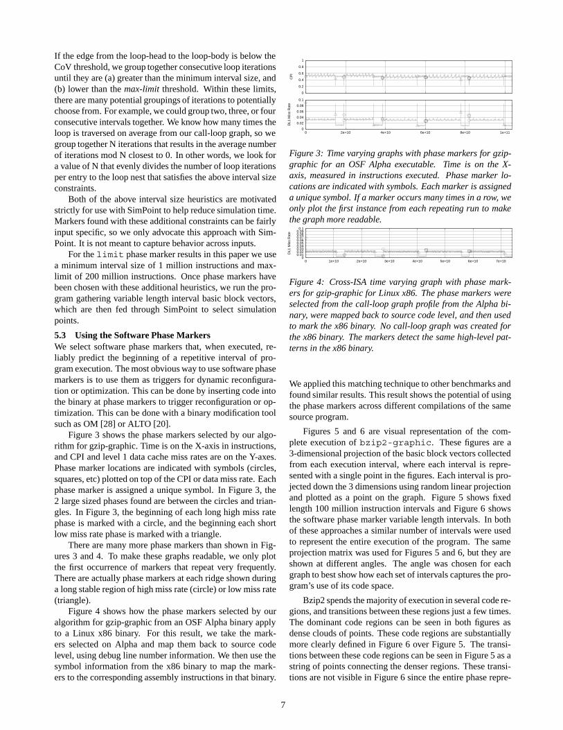
Figure 3 shows the phase markers selected by our algo-rithm for gzip-graphic. Time is on the X-axis in instructions,and CPI and level 1 data cache miss rates are on the Y-axes.Phase marker locations are indicated with symbols (circles,squares, etc) plotted on top of the CPI or data miss rate. Eachphase marker is assigned a unique symbol. In Figure 3, the2 large sized phases found are between the circles and trian-gles. In Figure 3, the beginning of each long high miss ratephase is marked with a circle, and the beginning each shortlow miss rate phase is marked with a triangle.

There are many more phase markers than shown in Fig-ures 3 and 4. To make these graphs readable, we only plotthe first occurrence of markers that repeat very frequently.There are actually phase markers at each ridge shown duringa long stable region of high miss rate (circle) or low miss rate(triangle).

Figure 4 shows how the phase markers selected by ouralgorithm for gzip-graphic from an OSF Alpha binary applyto a Linux x86 binary. For this result, we take the mark-ers selected on Alpha and map them back to source codelevel, using debug line number information. We then use thesymbol information from the x86 binary to map the mark-ers to the corresponding assembly instructions in that binary.

0

0.2

0.4

0.6

0.8

1

CP

I

0

0.02

0.04

0.06

0.08

0.1

0 2e+10 4e+10 6e+10 8e+10 1e+11

DL1

Mis

s R

ate

Figure 3: Time varying graphs with phase markers for gzip-graphic for an OSF Alpha executable. Time is on the X-axis, measured in instructions executed. Phase marker lo-cations are indicated with symbols. Each marker is assigneda unique symbol. If a marker occurs many times in a row, weonly plot the first instance from each repeating run to makethe graph more readable.

0 0.01 0.02 0.03 0.04 0.05 0.06 0.07 0.08 0.09 0.1

0 1e+10 2e+10 3e+10 4e+10 5e+10 6e+10 7e+10

DL1

Mis

s R

ate

Figure 4: Cross-ISA time varying graph with phase mark-ers for gzip-graphic for Linux x86. The phase markers wereselected from the call-loop graph profile from the Alpha bi-nary, were mapped back to source code level, and then usedto mark the x86 binary. No call-loop graph was created forthe x86 binary. The markers detect the same high-level pat-terns in the x86 binary.

We applied this matching technique to other benchmarks andfound similar results. This result shows the potential of usingthe phase markers across different compilations of the samesource program.

Figures 5 and 6 are visual representation of the com-plete execution of bzip2-graphic. These figures are a3-dimensional projection of the basic block vectors collectedfrom each execution interval, where each interval is repre-sented with a single point in the figures. Each interval is pro-jected down the 3 dimensions using random linear projectionand plotted as a point on the graph. Figure 5 shows fixedlength 100 million instruction intervals and Figure 6 showsthe software phase marker variable length intervals. In bothof these approaches a similar number of intervals were usedto represent the entire execution of the program. The sameprojection matrix was used for Figures 5 and 6, but they areshown at different angles. The angle was chosen for eachgraph to best show how each set of intervals captures the pro-gram’s use of its code space.

Bzip2 spends the majority of execution in several code re-gions, and transitions between these regions just a few times.The dominant code regions can be seen in both figures asdense clouds of points. These code regions are substantiallymore clearly defined in Figure 6 over Figure 5. The transi-tions between these code regions can be seen in Figure 5 as astring of points connecting the denser regions. These transi-tions are not visible in Figure 6 since the entire phase repre-

7

-0.3 -0.2 -0.1 0 0.1 0.2 0.3 0.4-0.5

0

0.5

-0.8

-0.6

-0.4

-0.2

0

0.2

0.4

0.6

Figure 5: Bzip2 fixed length execution intervals rep-resentation. The scattered representation with pointsspread across the space is a direct consequence of us-ing fixed length intervals across the execution.

-0.6

-0.4

-0.2

0

-0.6 -0.4 -0.2 0 0.2 0.4 0.6

-0.2

-0.1

0

0.1

0.2

0.3

Figure 6: Bzip2 variable length execution intervalsrepresentation using our phase markers. The tightclustering of intervals is from marking regions of thehierarchical call-loop graph that have fairly homoge-neous behavior each time that edge is traversed duringexecution.

sentation is synchronized with the program behavior wheretransitions between dominant regions are encapsulated byunique intervals.

These figures provide visual evidence that software phasemarkers are partitioning the execution into naturally occur-ring intervals that are in the code. This representation is cap-turing a lot of periodic behavior in the program. On the otherhand, the fixed length intervals are ignorant of the underly-ing program behavior, and consequently are dissonant withperiodic behavior. That explains why visually the executionappears more chaotic with fixed length intervals.

5.4 Behavior Characteristics of Software Phase Mark-ers

In this subsection we present behavior results from using themarker selection algorithm. For these results, we set ilowerto 1M instructions. We experiment with selecting phasemarkers from the training input and applying the markers tothe ref input (cross-train), as well as selecting and applyingmarkers from the ref input (self-train). All numbers are re-ported running the ref input.

We compare the results of our phase marking algorithmto SimPoint 2.0 [25], an offline phase analysis tool based onthe k-means clustering algorithm from machine learning. Forexperiments with SimPoint, we collected basic block vec-tors with ten million instructions per interval, and ran Sim-Point on the vectors with a 15 dimension random projectionand kmax = 100. SimPoint classifies the intervals of ex-ecution into phases. Note this is an idealized comparison,since the SimPoint analysis cannot be used across inputs. We

also show experiments with allowing our phase marking al-gorithm to only mark procedures. The result is similar to theapproach of Huang et. al. [12] and that used by Georges et.al. [9], but we use our call-loop graph, instead of a dynamiccall stack approach used in their prior work. This allows usto mark the procedure call edges in the binary.

For our phase marker results, the no-limit results rep-resent creating phase markers using the algorithm as statedin Section 5.1 where we do not put an upper bound on themaximum interval length. In comparison, the result calledlimit 1-200m represents using the additional heuristicsin Section 5.2 to choose phase markers that constrain the sizeof the variable length intervals produced to be used by Sim-Point. For these results we used a minimum interval size of1 million instructions and max-limit of 200 million instruc-tions.

Figure 7 shows the average interval length selected byeach approach. BBV uses fixed-length 10M instruction in-tervals. The next two bars show the results using our phasemarking approach, but only looking at edges coming intoprocedure-heads and procedure-bodies in the call-loop graph.The last three bars show the results for choosing any edge inthe call-loop graph (marking both procedures and loops). Allexcept the last bar for the phase marker results choose phasemarkers without specifying a limit on the maximum intervalsize, whereas the last bar using a maximum limit of 200 mil-lion instructions. Bars that might look like they are missinghave an average interval size of 1 million instructions. Forthe self-train results, we examine a call-loop graph of the ref-

8

1

10

100

1000

10000

100000

art/1

10

bzip2

/gra

phic

galge

l/ref

gcc/1

66

gzip/

grap

hic

lucas

/ref

mcf/re

f

mgrid/

ref

perlb

mk/diffm

ail

vorte

x/one

vpr/r

oute av

g

Ave

rage

Inte

rval

Len

gth

In M

illio

ns

BBV no limit cross procs no limit self procs no limit cross no limit self limit 1-200m

Figure 7: Average instructions per interval. BBV uses fixed10M instruction intervals. The rest of the results use softwarephase markers without specifying a limit on the maximum in-terval size and the last bar using a limit of 200 million in-structions. The second and third bar only allow marking ofprocedures, whereas the last three bars can mark both proce-dures and loops.

0

20

40

60

80

100

120

art/1

10

bzip2

/gra

phic

galge

l/ref

gcc/1

66

gzip/

grap

hic

lucas

/ref

mcf/

ref

mgr

id/re

f

perlb

mk/d

iffmail

vorte

x/one

vpr/r

oute av

gNum

ber

of U

niqu

e P

hase

IDs BBV no limit cross procs no limit self procs no limit cross no limit self limit 1-200m

Figure 8: Number of phases detected

0%20%40%60%80%

100%120%140%

art/1

10

bzip2

/gra

phic

galge

l/ref

gcc/1

66

gzip/

grap

hic

lucas

/ref

mcf/

ref

mgr

id/re

f

perlb

mk/d

iffmail

vorte

x/one

vpr/r

oute av

g

CoV

CP

I

BBV no limit cross procs no limit self procs no limit crossno limit self limit 1-200m 100k whole program 10m whole program

Figure 9: Coefficient of variation of CPI. Whole Programshows each program’s variability assuming each interval isclassified into a single phase

erence input (self-train), and for (cross-train) we examine acall-loop graph from the training input and apply the markersto the ref input (cross-train). Using only procedures to markphases results in average interval sizes of 1 billion (self-train)to 10 billion (cross-train) on average. Loops bring the aver-age interval size down to 10-100 million. The last bar showsthat putting a limit on the size of the intervals when perform-ing the marking has an average interval size of 3 million in-structions.

Figure 8 shows the number of phases detected by eachapproach. The BBV approach detects the most phases, andit also has the lowest variation in phases as we will see inFigure 9. In most cases, our approach detects half as many

phases as the BBV approach. Finally, if we constrain thesearch space of the call-loop graph by limiting the intervalsizes considered for SimPoint, we end up with more phasemarkers.

Figure 9 shows the average coefficient of variation of CPIper phase. The last two bars in these graphs show the over-all program CoV using fixed length intervals of 100,000 in-structions and 10 million instructions. These graphs showthat both the BBV and our software phase marker approachsuccessfully partition execution into phases of homogeneousbehavior. The procedures-only results have a lower CoVCPI for some programs than when using loop and proce-dures. This occurs because marking procedures detects fewerphases and produces significantly larger intervals comparedto procedures and loops. The general trend we have found isthat more behavior variability must be tolerated with smallerinterval sizes. For example, it is easy to get a CoV of close tozero with a few number of phases: just treat the whole pro-gram as one big interval. This is essentially what happensfor a few programs (like vpr) for the procedure only results.In general, program behavior variability decreases as largerintervals of execution are examined. In all cases, the averagebehavior variation within each phase is much lower than theprogram’s overall behavior variability.

6 Applications: Data Cache Reconfiguration andSimPoint

In this section we examine applying our code phase markersto data cache reconfiguration as in [23] and to SimPoint asin [15].

6.1 Data Cache Reconfiguration and Comparison toData Reuse Markers

Adaptive data cache reconfiguration dynamically reduces thecache size to reduce energy consumption and access time,without increasing the miss rate. In this section we performthe exact same data cache reconfiguration experiment doneby Shen et. al. [23] to apply our software phase markersto data cache reconfiguration. To ensure that our results arecomparable to prior work, we obtained from Shen the bench-marks and simulation infrastructure used in [23] as discussedin Section 3. We also obtained from them their binaries andtheir data phase markers, and we simulate the same adaptivecache hardware: 64-byte blocks, 512 sets, 32KB to 256KBcache size. The cache reconfigures by changing associativityfrom 1 to 8 ways.

In using their approach (Shen et. al. [23]) for adaptivecache analysis, during execution the first two intervals foreach phase marker are spent experimenting with the differentcache configurations. In the first two intervals, the best cacheconfiguration is determined for the phase. After the first twointervals, when the phase marker is seen again, the best cacheconfiguration is automatically used for the interval. We applythe same algorithm with our software phase markers.

We compare their markers against an ideal SimPoint [25]approach. SimPoint is an offline phase analysis tool basedon the k-means clustering algorithm from machine learning.

9

0

64

128

192

256

applu compress mesh swim tomcatv avg

Ave

rage

Cac

he S

ize

(KB

)BBV Reuse DistanceSPM-Self SPM-CrossProcs-Cross Best Fixed Size

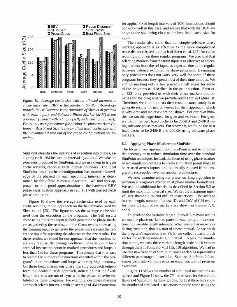
Figure 10: Average cache size with no allowed increase incache miss rate. BBV is the idealistic SimPoint-based ap-proach, Reuse Distance is the approach of Shen et al (trainedwith train input), and Software Phase Marker (SPM) is ourapproach (trained with ref input (self) and train input(cross)).Procs only uses procedures for picking the phase markers (noloops). Best Fixed Size is the smallest fixed cache size withthe maximum hit rate out of the cache configurations we ex-amine.

SimPoint classifies the intervals of execution into phases, as-signing each 10M instruction interval a phaseid. We take thephaseids produced by SimPoint, and we use them to triggercache reconfiguration at each interval boundary. The idealSimPoint-based cache reconfiguration has oracular knowl-edge of the phaseid for each upcoming interval, as deter-mined by the offline k-means algorithm. We find this ap-proach to be a good approximation to the hardware BBVphase classification approach in [26, 17] with perfect next-phase prediction.

Figure 10 shows the average cache size used by eachcache reconfiguration approach on the benchmarks used byShen et. al. [23]. The figure shows the average cache sizeused over the execution of the program. The Self resultsshow using the same input to both generate the phase mark-ers as gathering the results, and the Cross results show usingthe training input to generate the phase markers and the ref-erence input for reporting the adaptive cache size results. Forthese results, we found for our approach that the benchmarksare very regular: the average coefficient of variation of hier-archical instruction count in marked procedures and loops isless than 1% for these programs. This means that it is easyto predict the number of instructions executed within the pro-gram’s main procedures and loops with very high accuracy.On these benchmarks, our phase marking approach outper-form the idealistic BBV approach, indicating that the fixed-length intervals are out of sync with the phase behavior ex-hibited by these programs. For example, our phase markingapproach selects intervals with an average of 4M instructions

for applu. Fixed length intervals of 10M instructions shouldnot work well in this case, and we see that with the BBV av-erage cache size being close to the best fixed cache size forapplu.

The results also show that our simple software phasemarking approach is as effective as the more complicatedreuse distance-based approach of Shen et. al. [23] for cachereconfiguration on these regular programs. We also find thatselecting markers from the train input is as effective as select-ing markers from the ref input, as expected due to the regularbehavior patterns exhibited by these programs. Examiningonly procedures does not work very well for some of theseprograms because they spend most of their time in loops. Weend up marking only a few procedure call edges for someof the programs as described in the prior section. Shen et.al. [23] only provided us with their phase markers and bi-naries for the programs we provide results for in Figure 10.Therefore, we could not run their reuse-distance analysis togenerate results for gcc or vortex for their approach, whichis why gcc and vortex are not shown. For our own bina-ries we ran this experiment for gcc and vortex. For gcc,we found the best fixed cache to be 256KB and 240KB us-ing software phase markers. For vortex, we found the bestfixed cache to be 245KB and 200KB using software phasemarkers.

6.2 Applying Phase Markers to SimPointThe focus of our approach with SimPoint is not to improvethe accuracy or to reduce simulation time over the standardSimPoint technique. Instead, the focus of using phase-markerbased simulation points is to create simulation points that canbe re-used across inputs, and potentially re-used if the pro-gram is recompiled, even on another architecture.

We now examine using our phase marking algorithm topartition a program’s execution at phase marker boundaries.We use the additional heuristics described in Section 5.2 tolimit the maximum interval size. We set the maximum inter-val size threshold to 200 million instructions. The averageinterval length, number of phase IDs and CoV of CPI resultsfor these limit phase markers are shown in Figures 7, 8,and 9.

To produce the variable length interval SimPoint resultswe use the phase markers to partition each program’s execu-tion into variable length intervals. Whenever a marker occursduring execution, that is a start of a new interval. As we breakthe program’s execution into VLIs, we collect a basic blockvector for each variable-length interval. To pick the simula-tion points, we pass these variable length basic block vectorsthrough the SimPoint 3.0 VLI [15, 10] algorithm. We had touse this new version of SimPoint, since each VLI represents adifferent percentage of execution. Standard SimPoint 2.0 as-sumes each interval represents an equal fraction of programexecution.

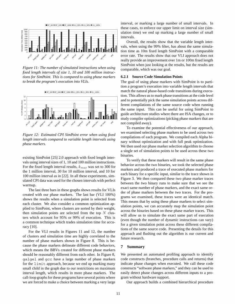
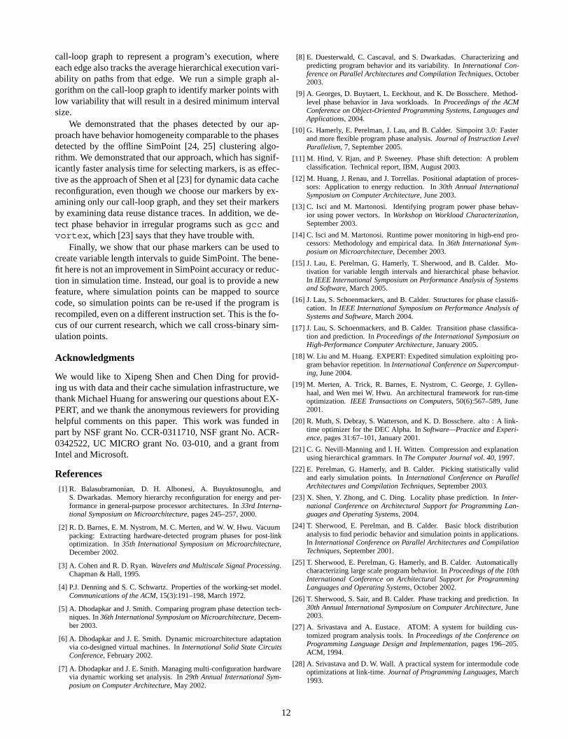
Figure 11 shows the number of simulated instructions re-quired, and Figure 12 show the CPI error rates for the variousflavors of SimPoint. In these graphs, the first three bars showthe number of simulated instructions required when using the

10

0100200300400500600700800900

1000

art.1

10

bzip2

.grp

h

galge

l.ref

gcc.1

66

gzip.

grph

lucas

.ref

mcf.

ref

mgr

id.re

f

perl.

diff

vorte

x.one

vpr.r

oute av

g

Sim

ulat

ion

Tim

e (M

illio

n In

st)

SP_1M SP_10M SP_100M VLI_95% VLI_99% VLI_100%

Figure 11: The number of simulated instructions when usingfixed length intervals of size 1, 10 and 100 million instruc-tions for SimPoint. This is compared to using phase markersto break the program’s execution into VLIs.

0

2

4

6

8

10

12

art.1

10

bzip2

.grp

h

galge

l.ref

gcc.1

66

gzip.

grph

lucas

.ref

mcf.

ref

mgr

id.re

f

perl.

diff

vorte

x.one

vpr.r

oute av

g

% C

PI R

elat

ive

Err

or

SP_1M SP_10M SP_100M VLI_95% VLI_99% VLI_100%

Figure 12: Estimated CPI SimPoint error when using fixedlength intervals compared to variable length intervals usingphase markers.

existing SimPoint [25] 2.0 approach with fixed length inter-vals using interval sizes of 1, 10 and 100 million instructions.For the fixed length interval results, kmax was set to 300 forthe 1 million interval, 30 for 10 million interval, and 10 for100 million interval as in [22]. In all these experiments, sim-ulated CPI data was used for the chosen intervals with perfectwarmup.

The last three bars in these graphs shows results for VLIscreated with our phase markers. The last bar (VLI 100%)shows the results when a simulation point is selected fromeach cluster. We also consider a common optimization ap-plied to SimPoint, where clusters are sorted by their weight,then simulation points are selected from the top N clus-ters which account for 95% or 99% of execution. This isa common technique which trades simulation time for accu-racy [10].

For the VLI results in Figures 11 and 12, the numberof clusters and simulation time are highly correlated to thenumber of phase markers shown in Figure 8. This is be-cause the phase markers delineate different code behaviors,which means the BBVs created for different phase markersshould be reasonably different from each other. In Figure 8,galgel and gcc have a large number of phase markersfor the limit approach, because we end up marking manysmall child in the graph due to our restrictions on maximuminterval length, which results in more phase markers. Thecall-loop graphs for these programs have several points wherewe are forced to make a choice between marking a very large

interval, or marking a large number of small intervals. Inthese cases, to enforce our upper limit on interval size (sim-ulation time) we end up marking a large number of smallintervals.

Overall, the results show that the variable length inter-vals, when using the 99% filter, has about the same simula-tion time as 10m fixed length SimPoint with a comparableerror rate. The results show that our VLI approach does notreally provide an improvement over 1m or 100m fixed lengthSimPoint when just looking at the results, but the results arecomparable, which was our goal.

6.2.1 Source Code Simulation PointsThe goal of using phase markers with SimPoint is to parti-tion a program’s execution into variable length intervals thatmatch the natural phase-based code transitions during execu-tion. This allows us to mark phase transitions at the code leveland to potentially pick the same simulation points across dif-ferent compilations of the same source code when runningthe same input. This can be useful for using SimPoint toguide architecture studies where there are ISA changes, or tostudy compiler optimizations (picking phase markers that arenot compiled away).

To examine the potential effectiveness of our approach,we examined selecting phase markers to be used across twocompilations of each program. We compiled each Alpha bi-nary without optimization and with full peak optimization.We then used our phase marker selection algorithm to choosea single set of simulation points to be used across these twobinaries.

To verify that these markers will result in the same phasebehavior across the two binaries, we took the selected phasemarkers and produced a trace of executed phase markers foreach binary for a specific input, similar to the trace shown inFigure 3. We then compared these two phase marker tracesbetween the two binary runs to make sure that we see theexact same number of phase markers, and the exact same or-der of phase markers between the two traces. For the pro-grams we examined, these traces were an identical match.This means that by using these phase markers to select sim-ulation points, we can accurately map the simulation pointacross the binaries based on these phase marker traces. Thiswill allow us to simulate the exact same part of execution(even though the number of dynamic instructions can vary)for a given simulation point across these different compila-tions of the same source code. Presenting the details for thisapproach and flushing out the algorithm is our current andfuture research.

7 Summary

We presented an automated profiling approach to identifycode constructs (branches, procedure calls and returns) thatindicate phase changes when executed. We call these codeconstructs “software phase markers,” and they can be used toeasily detect phase changes across different inputs to a pro-gram without hardware support.

Our approach builds a combined hierarchical procedure

11

call-loop graph to represent a program’s execution, whereeach edge also tracks the average hierarchical execution vari-ability on paths from that edge. We run a simple graph al-gorithm on the call-loop graph to identify marker points withlow variability that will result in a desired minimum intervalsize.

We demonstrated that the phases detected by our ap-proach have behavior homogeneity comparable to the phasesdetected by the offline SimPoint [24, 25] clustering algo-rithm. We demonstrated that our approach, which has signif-icantly faster analysis time for selecting markers, is as effec-tive as the approach of Shen et al [23] for dynamic data cachereconfiguration, even though we choose our markers by ex-amining only our call-loop graph, and they set their markersby examining data reuse distance traces. In addition, we de-tect phase behavior in irregular programs such as gcc andvortex, which [23] says that they have trouble with.

Finally, we show that our phase markers can be used tocreate variable length intervals to guide SimPoint. The bene-fit here is not an improvement in SimPoint accuracy or reduc-tion in simulation time. Instead, our goal is to provide a newfeature, where simulation points can be mapped to sourcecode, so simulation points can be re-used if the program isrecompiled, even on a different instruction set. This is the fo-cus of our current research, which we call cross-binary sim-ulation points.

Acknowledgments

We would like to Xipeng Shen and Chen Ding for provid-ing us with data and their cache simulation infrastructure, wethank Michael Huang for answering our questions about EX-PERT, and we thank the anonymous reviewers for providinghelpful comments on this paper. This work was funded inpart by NSF grant No. CCR-0311710, NSF grant No. ACR-0342522, UC MICRO grant No. 03-010, and a grant fromIntel and Microsoft.

References[1] R. Balasubramonian, D. H. Albonesi, A. Buyuktosunoglu, and

S. Dwarkadas. Memory hierarchy reconfiguration for energy and per-formance in general-purpose processor architectures. In 33rd Interna-tional Symposium on Microarchitecture, pages 245–257, 2000.

[2] R. D. Barnes, E. M. Nystrom, M. C. Merten, and W. W. Hwu. Vacuumpacking: Extracting hardware-detected program phases for post-linkoptimization. In 35th International Symposium on Microarchitecture,December 2002.

[3] A. Cohen and R. D. Ryan. Wavelets and Multiscale Signal Processing.Chapman & Hall, 1995.

[4] P.J. Denning and S. C. Schwartz. Properties of the working-set model.Communications of the ACM, 15(3):191–198, March 1972.

[5] A. Dhodapkar and J. Smith. Comparing program phase detection tech-niques. In 36th International Symposium on Microarchitecture, Decem-ber 2003.

[6] A. Dhodapkar and J. E. Smith. Dynamic microarchitecture adaptationvia co-designed virtual machines. In International Solid State CircuitsConference, February 2002.

[7] A. Dhodapkar and J. E. Smith. Managing multi-configuration hardwarevia dynamic working set analysis. In 29th Annual International Sym-posium on Computer Architecture, May 2002.

[8] E. Duesterwald, C. Cascaval, and S. Dwarkadas. Characterizing andpredicting program behavior and its variability. In International Con-ference on Parallel Architectures and Compilation Techniques, October2003.

[9] A. Georges, D. Buytaert, L. Eeckhout, and K. De Bosschere. Method-level phase behavior in Java workloads. In Proceedings of the ACMConference on Object-Oriented Programming Systems, Languages andApplications, 2004.

[10] G. Hamerly, E. Perelman, J. Lau, and B. Calder. Simpoint 3.0: Fasterand more flexible program phase analysis. Journal of Instruction LevelParallelism, 7, September 2005.

[11] M. Hind, V. Rjan, and P. Sweeney. Phase shift detection: A problemclassification. Technical report, IBM, August 2003.

[12] M. Huang, J. Renau, and J. Torrellas. Positional adaptation of proces-sors: Application to energy reduction. In 30th Annual InternationalSymposium on Computer Architecture, June 2003.

[13] C. Isci and M. Martonosi. Identifying program power phase behav-ior using power vectors. In Workshop on Workload Characterization,September 2003.

[14] C. Isci and M. Martonosi. Runtime power monitoring in high-end pro-cessors: Methodology and empirical data. In 36th International Sym-posium on Microarchitecture, December 2003.

[15] J. Lau, E. Perelman, G. Hamerly, T. Sherwood, and B. Calder. Mo-tivation for variable length intervals and hierarchical phase behavior.In IEEE International Symposium on Performance Analysis of Systemsand Software, March 2005.

[16] J. Lau, S. Schoenmackers, and B. Calder. Structures for phase classifi-cation. In IEEE International Symposium on Performance Analysis ofSystems and Software, March 2004.

[17] J. Lau, S. Schoenmackers, and B. Calder. Transition phase classifica-tion and prediction. In Proceedings of the International Symposium onHigh-Performance Computer Architecture, January 2005.

[18] W. Liu and M. Huang. EXPERT: Expedited simulation exploiting pro-gram behavior repetition. In International Conference on Supercomput-ing, June 2004.

[19] M. Merten, A. Trick, R. Barnes, E. Nystrom, C. George, J. Gyllen-haal, and Wen mei W. Hwu. An architectural framework for run-timeoptimization. IEEE Transactions on Computers, 50(6):567–589, June2001.

[20] R. Muth, S. Debray, S. Watterson, and K. D. Bosschere. alto : A link-time optimizer for the DEC Alpha. In Software—Practice and Experi-ence, pages 31:67–101, January 2001.

[21] C. G. Nevill-Manning and I. H. Witten. Compression and explanationusing hierarchical grammars. In The Computer Journal vol. 40, 1997.

[22] E. Perelman, G. Hamerly, and B. Calder. Picking statistically validand early simulation points. In International Conference on ParallelArchitectures and Compilation Techniques, September 2003.

[23] X. Shen, Y. Zhong, and C. Ding. Locality phase prediction. In Inter-national Conference on Architectural Support for Programming Lan-guages and Operating Systems, 2004.

[24] T. Sherwood, E. Perelman, and B. Calder. Basic block distributionanalysis to find periodic behavior and simulation points in applications.In International Conference on Parallel Architectures and CompilationTechniques, September 2001.

[25] T. Sherwood, E. Perelman, G. Hamerly, and B. Calder. Automaticallycharacterizing large scale program behavior. In Proceedings of the 10thInternational Conference on Architectural Support for ProgrammingLanguages and Operating Systems, October 2002.

[26] T. Sherwood, S. Sair, and B. Calder. Phase tracking and prediction. In30th Annual International Symposium on Computer Architecture, June2003.

[27] A. Srivastava and A. Eustace. ATOM: A system for building cus-tomized program analysis tools. In Proceedings of the Conference onProgramming Language Design and Implementation, pages 196–205.ACM, 1994.

[28] A. Srivastava and D. W. Wall. A practical system for intermodule codeoptimizations at link-time. Journal of Programming Languages, March1993.

12