Seismo-volcano source localization with triaxial

broad-band seismic array

Adolfo Inza, Jerome Mars, Jean-Philippe Metaxian, Gareth S. O’Brien,

Orlando Macedo

To cite this version:

Adolfo Inza, Jerome Mars, Jean-Philippe Metaxian, Gareth S. O’Brien, Orlando Macedo.Seismo-volcano source localization with triaxial broad-band seismic array. Geophysical JournalInternational, Oxford University Press (OUP), 2011, 187 (1), pp.371-384. <10.1111/j.1365-246X.2011.05148.x>. <hal-00625252>

HAL Id: hal-00625252

https://hal.archives-ouvertes.fr/hal-00625252

Submitted on 21 Sep 2011

HAL is a multi-disciplinary open accessarchive for the deposit and dissemination of sci-entific research documents, whether they are pub-lished or not. The documents may come fromteaching and research institutions in France orabroad, or from public or private research centers.

L’archive ouverte pluridisciplinaire HAL, estdestinee au depot et a la diffusion de documentsscientifiques de niveau recherche, publies ou non,emanant des etablissements d’enseignement et derecherche francais ou etrangers, des laboratoirespublics ou prives.

Geophys. J. Int.(2003)000, 000–000

Seismo-Volcano Source Localization withTriaxial-Broadband Seismic Array

L. A. Inza1,2,4, J.I. Mars1, J. P. Metaxian2, G. S O’Brien3 and O. Macedo41 GIPSA-LAB/DIS/UMR 5216 Institute Polytechnique de Grenoble, FRANCE2 Laboratoire de Geophysique Interne et Tectonophysique IRD:R157 CNRS, Universite de Savoie, FRANCE3 School of Geological Science, University College Dublin IRELAND4 Instituto Geofisico del Peru, IGP PERU

Received 2010 September 18; in original form 2010 September5

SUMMARYSeismo-volcano source localization is essential to improve our understanding of eruptive dy-namics and of magmatic systems. The lack of clear seismic wave phases prohibits the useof classical location methods. Seismic antennas composed of one-component (1C) seismome-ters provide a good estimate of the back-azimuth of the wavefield. The depth estimation, onthe other hand, is difficult or impossible to determine. As inclassical seismology, the use ofthree component (3C) seismometers is now common in volcano studies. In order to determinethe source location parameters (back-azimuth and depth), we extend the 1C seismic antennaapproach to 3C’s. This article discusses a high-resolutionlocation method using a 3C arraysurvey (3C MUSIC algorithm) with data from two seismic antennas installed on an andesiticvolcano in Peru (Ubinas volcano). One of the main scientific questions related to the eruptiveprocess of Ubinas volcano is the relationship between the magmatic explosive and LP swarms.After introducing the 3C array theory, we evaluate the robustness of the location method ona full wavefield 3D synthetic dataset generated using a digital elevation model of Ubinas vol-cano and a heterogeneous velocity model obtained from a tomography study. Results show thatthe back-azimuth determined using the 3C array has a smallererror than a 1C array. Only the3C method allows the recovery of the source depths. Finally,we applied the 3C approach to aseismic event recorded in 2009. Crossing the estimated back-azimuth and incidence angles, wefind a source located 1000±250 m below the bottom the active crater. Therefore, extending 1Carrays to 3C arrays in volcano monitoring allows a more accurate determination of the sourceepicenter and now an estimate for the depth.

Key words: Spatial analysis, Volcan monitoring, Fourier analysis, Time series analysis, Seis-mic array analysis.

1 INTRODUCTION

Source location (back-azimuth and depth determination) isa fun-damental goal in volcano monitoring. Long-period (LP) events andtremor, which are directly related to magma ascent, constitute themain classes of seismic events observed on andesitic volcanoes(Chouet, 1996). Locating these events is therefore necessary to bet-ter understand the eruptive dynamics and to improve the knowledgeof the magmatic system. The lack of clear body-wave phase arrivalsand emergent onsets in LP events and tremor makes locating theseevents extremely difficult using classical hypocenter determinationmethods based on phase picking and calculation of travel times.Other location methods have been used in recent years including amethod based on the spatial distribution of seismic amplitudes tolocate eruptive tremor sources on the Piton de la Fournaise volcano(Battaglia & Aki, 2003) and to track tremors produced by lahars onCotopaxi volcano (Hiroyuki et al., 2009). Dense one-component

(1C) array methods based on time delays between close sensors,hence an estimation of the slowness vector of the wavefrontsprop-agating across the array, have been used by several authors and ap-plied to a great variety of volcanoes. For example (Saccorotti &DelPezzo, 2000) and (La Rocca et al., 2004) applied dense one-component array techniques to locate explosive activity atStrom-boli. (Almendros et al., 2002) characterized the spatial extent ofa hydrothermal system at Kilauea volcano by using similar tech-niques. (Metaxian et al., 2002) used several small dense arrays tolocate LP events and tremor sources at Arenal volcano and (DiLi-eto et al., 2007) used two dense one-component arrays of shortperiod seismometers to track volcanic tremor at Etna. Denseone-component array methods usually consist of only the vertical seis-mic component and allow a good estimation of the back-azimuthof the wavefield. Unfortunately, the depth estimation is poorly re-solved because the incidence angle is very difficult to determine.To overcome this problem, triaxial sensors (3C) can be used.In

2

this work we focus on the gain in back-azimuth resolution anddepth determination obtained by three-component rather than one-component seismometers. In our study two 3C arrays were installedon Ubinas volcano, Peru, in March 2009 in order to determine theback-azimuth and depth of the seismo-volcano sources. The twosmall-aperture cross-shaped seismic arrays consisted of 12 three-component broadband seismometers. One of the main scientificquestions related to the eruptive process at Ubinas is the relation-ship between the magmatic explosions and the LP swarms preced-ing these events by several tens of minutes to a few hours (Macedoet al., 2009). Source location of the LP events with a higher resolu-tion compared to the one component dense array methods, particu-larly in the depth determination, is the main objective of this work.To achieve this goal and before working with real wavefield datawe performed several numerical simulations of seismic waveprop-agation using a 3D digital elevation map and heterogeneous veloc-ity model determined from a tomography study, (Monteiller et al.,2005). Sources were placed at different depths below the crater andreceivers are situated at the same positions as the two experimentalcross-shaped arrays. A high-resolution method based on themul-tiple signal classification (MUSIC technique) (Bienvenu & Kopp,1983), (Schmidt, 1986), but adapted to the 3C case, is applied tothe synthetic data to determine the back-azimuth, the apparent ve-locity and the incidence angle for both arrays and all sources. Thisprocedure is then applied to the real data recorded in March 2009.

2 UBINAS VOLCANO

Ubinas volcano (16 22’ S, 70 54’ W; altitude 5672 m) began toerupt on March 25th 2006 after nearly 40 years of quiescence. Sit-uated in the Central Volcanic Zone (CVZ, southern Peru), Ubinasvolcano is an active andesitic stratovolcano (De Silva & Francis,1991) truncated in the upper part by a caldera 600 m in diame-ter. The caldera floor is a flat area lying approximately 5100 mabove sea level. The active crater is situated in the southern section;the bottom is 300 m under the caldera floor (Figure 1a). Ubinasisconsidered the most active Peruvian volcano during the last500years, threatening 3,500 people living on the edge of the Ubinasrio (Rivera et al., 1998). Arequipa airport, situated 60 km east ofthe volcano, has been closed several times since 2006 due to ashemissions. The Instituto Geofisico del Peru (IGP) with the cooper-ation of the Institut de Recherche pour le Developement (IRD) hasstarted seismic monitoring of the volcano to understand theactivityassociated with this eruptive sequence under the 6th framework EUproject VOLUME (http://www.volume-project.net/). A network offour digital 1 Hz stations with a radio telemetry system has beenoperating since 2006. Data are transmitted to Arequipa observa-tory. At the time of the experiment, the eruption was characterizedby an almost permanent ash emission. Two main types of degasi-fication were observed: 1) exhalations rising a few hundred metersabove the crater rim and 2) plumes produced by explosions thatmay reach 10 km, critical for aircraft duty. This activity isthoughtto be related to a magmatic plug positioned at the bottom of thesouth part of the caldera wall (Macedo et al., 2009).

3 PROCESSING APPROACH

Three component broadband seismic array data is suitable for wide-band multidimensional signal processing techniques. The antennais designed (size, shape, aperture) to avoid spatial and temporal

aliasing (Mars et al., 2004). To illustrate the 3C MUSIC method,we assume an isotropic source radiation pattern and a homoge-neous medium. Assuming K sources impinging at the antenna ofN triaxial sensors, equation (1) represents the received signal bynth sensor in time-space(t − x) domain.

xn(t) =KX

k=1

sk(t − τn,k) + bn(t); n = 0, 1, ..., N − 1 (1)

where,sk(t) is thekth source signal received in the first sensor,theτn,k is the relative propagation time delay ofkth source for thenth sensor and thebn(t) represents the noise innth sensor (we as-sume white noise and Gaussian with varianceσ2 and uncorrelatedwith the sources). The corresponding relative time delay isdefinedasτn,k = 1

v0[rn · u(θk, φk)] where,v0 is the wave propagation

apparent velocity beneath the array, thern is the relative locationfor sensornth respect to the first sensor located at (0,0,0) and theu(θk, φk) is the slowness vector of the impinging wavefield fromkth source. The dot product(rn · u) represents the propagationpath between thenth sensor respect to the first sensor. The propa-gation directionu(θk, φk) of thekth source arrived in the antennacan be described by back-azimuth angleθk and vertical incidenceangleφk, these two parameters are combined in the slowness vectoras is shown in equation (2).

u(θk, φk) =

24−sinθksinφk

−cosθksinφk

cosφk

35 (2)

Taking into account the wavenumberk, that is related ask =1

λw

u = fo

vo

u, where,λw is the wavelength,fo the wave frequencyand vo is the wave propagation apparent velocity. The Fouriertransform in equation (1) can be represented in the frequency-wavenumber(f − k) domain as:

Xn(fo) =

KX

k=1

Sk(fo)exp(−2πjrn · k) + Bn(fo) (3)

where,j =√−1 is the imaginary unit, andSk(f) and Bn(f)

are the Fourier transform ofsk(t) andbn(t) respectively. Then theantenna outputX(fo) for narrowband signals can be representedas a Nx1 matrix form as:

X(fo) = A(fo) · S(fo) + B(fo) (4)

where, the NxK matrixA(fo) is called “array reponse” or “steeringmatrix”, the Kx1 matrixS(fo) keeps the sources signals defined in(5), so the Nx1 matrixB(fo) represents the noise.

A(fo) = [a(θ1, φ1), a(θ2, φ2), ..., a(θK , φK)] (5)

a(θ, φ) =

2664

1exp(−j2πr1 · k)

.......exp(−j2πrN−1 · k)

3775

S(fo) = [s1(fo), ..., sK(fo)]T

Note that the array manifold a(θ, φ) depends on the frequencyfo

of the signal through the wavenumberk. The purpose of this paperis to develop and test a 3C MUSIC algorithm in order obtain amore robust estimation of the back-azimuth angleθ and a reliableincidence angleφ related to source depth determination.

3

3.1 3C MUSIC algorithm

MUltiple SIgnal Classification is an eigenstructure subspace anal-ysis method, that is widely used in geophysics, particularly to en-hance the signal-to-noise ratio. MUSIC algorithm tries to find thearray manifold orthogonal to the noise subspace since the noisesubspace is orthogonal to the signal subspace (Mars et al., 2004).A time window array data is selected, correspondig to eitherexplo-sion quakes or LP events. A way to find out the dominants frequen-cies in the wavefield is through average energy spectrum of eachcomponent, which the analysis frequencyfo is determined. Ob-serving M frequencies snapshots around the binfo (energy peak)are used to estimate the cross-spectral matrix. Theith snapshot datais shown in equation (6) defined by a NxM matrix (Paulus & Mars,2006).

Xi =

2664

WEi,1 SNi,1 Zi,1

. . .

. . .WEi,N SNi,N Zi,N

3775 ; i = 1, ..., M (6)

where, the triaxial sensor is represented by: the west-eastcom-ponent asWE, south-north asSN and vertical asZ. The cross-spectral matrixbΓ can be estimated using the equation (7) (Pauluset al., 2005) and .

bΓx =1

M

MX

i=1

Xi · XHi (7)

whereH denotes conjugate transpose. The cross-spectral matrix in(7) can be expressed in terms of its N eigenvalues and eigenvectors(N=sensors number), as shown the equations (8).

bΓx (ν) =

NX

n=1

λnvn · vH

n (8)

where,λn andvn are thenth eigenvalue and eigenvector respec-tively. Anyway the sample cross-spectral matrix is the expectedvalue of the outer product of the data vector. Using the orthogo-nality property between signal and noise subspaces, in the equation(4), the cross-spectral matrixΓx can be written as:

Γx = A · E{S · SH} · AH + E{B · BH} (9)

Γx (fo) = A (fo)Γs (fo)AH (fo) + σ2

B (fo) I

where, E{·} the expected operator,Γs (fo) is the signal cross-spectral matrix,I is the identity matrix andσ2

B is the varianceof the Gaussian white noise. This decomposition can be splitintotwo orthogonal subspaces such as signal and noise. In this casethe cross-spectral matrix (9) is equal to the estimated cross-spectralmatrix in (7) and (8). Due to errors in the estimated cross-spectralmatrix, the eigenvalues of the noise subspace are no longer equalto σ2

B . Assuming K sources impinging the antenna of N sensors(K < N ), the eigenvectors whose eigenvalues are the K largesteigenvalues define the signal subspace and the remaining N-Keigenvectors define the noise subspace. The largest eigenvaluesare easily distinguishable from the rest in the eigenvaluesλi, asλ1 ≥ ... ≥ λK ≥ λK+1 > ... > λN ≈ σ2 shows the appropri-ate dimension of noise subspace on theN − K smallest. Then thenoise projector is defined by (Miron et al., 2005):

Π⊥ =

NX

k=K+1

vkvHk

and the MUSIC estimator is (Wong & Zoltowski, 2000):

3CMUSIC (θ, φ) =1

AH (θ, φ)Π⊥A (θ, φ)(10)

Then 3C MUSIC algorithm follows the procedure: 1) Selectionbytime windowing data for either a quake explosion or LP event.2)Average power spectra density to determine the frequenciesbinsand entimate the cross-spectral matrix. 3) Eigen structureanaly-sis to estimate the noise sub-space to build the noise projector. 4)Evaluate the 3C MUSIC estimator on slowness grid and velocitygrid where the estimator is maximum.

4 DATA

A seismic experiment was carried out at Ubinas volcano betweenMay and July 2009. We deployed two cross-shaped antennas withtriaxial-broadband seismometers as depicted in Figure 1a.NUBIantenna was installed on a flat area 4632 m above sea level. It con-sists of twelve Guralp CMG-6TD seismometers (see referenceforGuralp manual). WUBI antenna was installed on a sloping areafrom 4752 m to 4883 m above sea level. It consists of six Gu-ralp CMG-6TD and six GEOMAX seismometers (see referencefor Geomax manual) both with 24 bit seismic recorders (dynamicrange 120 dB) and high accuracy time synchronization, GPS-based.The acquisition performed continuous recording with a samplingfrequency of a 100 Hz. The horizontal components of such seis-mometers were oriented to geographical coordinates West-East (Ecomponent) and South-North (N component) respectively. The dis-tances between seismometers was set to approximately 50 meters.Each seismometer location was surveyed by Trimble GPS (GeoXH,accuracy 0.3 m). Twelve explosion quakes and hundreds of LPevents were recorded during the experiment. A synthetic datasetwas generated to test the accuracy of the location methods. Thesynthetic dataset was created using a digital elevation mapof Ubi-nas topography and the 2009 experimental array locations. A3Ddiscrete numerical elastic lattice method (O’Brien & Bean,2004)was used to propagate waves in the structure with six broadbandisotropic sources (Figure 1b) located beneath the summit. The ve-locity structure was generated from a tomography study (Mon-teiller et al., 2005) assuming a density of 2300kg/m3. The sam-pling frequency was fixed to 250 Hz.

4.1 Synthetic data analysis

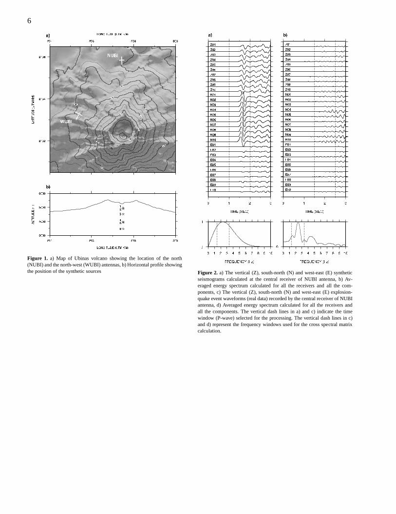
To investigate the performance of the 3C MUSIC technique, weap-plied it to our synthetic dataset. For source number 3 (Figure 1b)and the synthetic array NUBI a one second time window includingthe first arrival was selected, Figure 2a. In order to find the domi-nant frequency, we averaged the power spectral density computedfor the selected time window of each component and for each re-ceiver. The dominant energy peak is located at 2.23 Hz (Figure 2b).The cross-spectral matrix was then calculated by using 32 windowsaround the bin. The eigendecomposition of the cross-spectral ma-trix gave us an overview of the signal-to-noise subspaces, by sort-ing the eigenvalues. In the first stage, we determined the eigenvec-tors corresponding to the noise subspace, which gives the projector.In the second stage, we calculated the steering vector whichcon-sists of the slowness vector estimated between0 and2π with stepsof 3.6◦. Given the projector and the steering vector, we obtainedthe 3C MUSIC spectrum represented in Figure 3a. The maximum

4

amplitude of the spectrum gives the back-azimuth and the veloci-ties. The largest estimator point is located at 181±3◦ for the back-azimuth and 2900±75 m/s for the velocity. The vertical and hori-zontal cross-section of the 3C MUSIC spectrum are shown in Fig-ures 3b and 3c. The incidence angle is deduced from the estimatedvalues, back-azimuth and velocity. We found 85.5±6◦ as shown inFigure 3d. The errors are estimated by taking the peak width of95% of the maximum amplitude. These values agree well with thetheoretical values.

We applied the same analysis to the synthetic data generatedfor both arrays and for all six sources. In order to compare the 3Cand 1C methods, we also analyzed the same synthetic dataset usingonly the vertical components. The results are shown in the Fig-ure 4a and Figure 4b for NUBI and WUBI antennas respectively.Back-azimuth results obtained both with the 3C MUSIC and the1C MUSIC fit well with the theoretical values for both antennas.Errors are±3◦ and±6◦, with the 3C and the 1C MUSIC algo-rithm respectively. However, the incidence angles are significantlydifferent when using the 3C MUSIC and the 1C MUSIC analysis.For NUBI, values vary from 75◦ for the deepest source to 93◦ forsource 1. These incident angle variations are coherent withthe vari-ation of the sources depth. Errors are±6◦ for the 3C MUSIC anal-ysis. These errors allow us to distinguish sources depths separatedby several hundreds of meters but unable to separate close sourcessuch as 1 and 2 or sources 4 and 5. The 1C MUSIC analysis givessources close to the theoretical values for the superficial sources(1, 2 and 3) while depths for sources 4, 5 and 6 are far away fromthe theoretical values. The incident angle remains approximatelythe same value around 90◦. The error obtained with the 1C MUSICprocessing is±12◦. None of the sources can be distinguished withthe 1C MUSIC analysis. For WUBI antenna, the 3C MUSIC anal-ysis gives incident angles between 63◦ for source 6 and 100◦ forsource 2 (Figure 4b). As for NUBI, solutions follow the depthvari-ation. Error are approximately 6◦. The 1C MUSIC analysis giveshigher incident angles than the theoretical values (90◦ for source6 to 156◦ for source 1). Errors are larger than the 3C algorithm atapproximately±15◦. The 1C MUSIC analysis does not give reli-able solutions for any of the synthetic source depths. In this case, itseems that the solutions are affected by the topography below theantenna. Similar results are observed for the velocity. In summary,incident angles obtained by the 3C MUSIC algorithm are closetothe theoretical values whereas those obtained with 1C MUSICarenot reliable.

4.2 Real Data Analysis

In this section, we discuss the performance of 3C MUSIC methodby applying it to an explosion quake signal recorded at Ubinas vol-cano. The selected event, recorded at 01:27 PM, June2nd, 2009is shown in Figure 2c (SHOW A LONGER TIME WINDOW OFTHE SIGNAL). The data was corrected for the instrument responseand bandpass filtered between 1 Hz - 10 Hz. Figure 2d shows theantenna energy spectrum average obtained from two seconds of sig-nal including the first arrival wave. The dominant peak is centredat 2.39 Hz. The results for NUBI antenna are presented in Figure3e, 3f, 3g and 3h). (IF YOU WANT TO SEND TO DIFFERENTJOURNAL I’D SEPARATE THE SYNTHETIC AND DATA FIG-URES) The maximum of the 3C MUSIC spectrum gives a back-azimuth of 184±5◦ , a velocity of 2975±125 m/s and an inci-dence angle of 85.9±7◦. For WUBI, we obtained a back-azimuthof 119±6◦, a velocity of 3100±120 m/s and an incidence angleof 75±7◦. The back-azimuth and the incident angle can be repre-

sented as gaussian variables with meanθ (0≤ θ ≤ 360◦) and φ(0≤ φ ≤ 120◦) and standard deviationsσθ andσφ correspondingto the values found in the analysis. This allows the definition of aprobability density function (PDF)ρ(θk) of the back-azimuth anda PDFρ(φk) of the incident angle for each array k.ρ1(θ

k) andρ1(φ

k) are shown in Figure 5 as rose diagrams in the horizontalplane for the back-azimuths and in the vertical planes oriented N-Sand W-E for the incident angle. The last step is to locate the sourceby using the information obtained at each antenna. For each pointwith geographical coordinates (x,y,z) in the source regionand eacharray k, the back-azimuthsθk(x, y, z) and the corresponding valueof ρ1(θ

k), as well as the incident angleφk(x, y, z) and the corre-sponding value ofρ1(φ

k) can be calculated. The PDF of the sourceposition is derived from the different PDF’s of the back-azimuthand the incident angle:

ρ2(x, y, z) =2Y

k=1

ρ1(θk(x, y, z)) · ρ1(φ

k(x, y, z)) (11)

The maximum likelihood of the PDFρ2 yields an estimate ofthe source location. We define the mean quadratic radius R =p

(σ21 + σ2

2 + σ23)/3, whereσ2

1 , σ22 andσ2

3 are the principal vari-ances ofρ2(x, y, z). Figure 5 shows the result obtained with theexplosion quake analysis. The source area is situated 150 m Westand 1000 m below the bottom of the crater at an altitude of 4200m, the radius R is 660 m.

5 CONCLUSIONS

We have presented a source localization method, 3C MUSIC, basedon the use of 3 component arrays and, for comparison, with the1C MUSIC used in previous studies on volcanoes (Saccoroti etal.(2006)). Synthetics have been generated for 6 sources with eleva-tions from 3400 m to 4950 m a.s.l. The back-azimuths from the 3CMUSIC correspond to the theoretical values for both antennas witha resolution of±3◦. 1C MUSIC gives equivalent results, but withhigher errors (±6◦). The incident angle varies with depth when it isdetermined with 3C MUSIC. The incident angle is determined withan error of±6◦ for NUBI and for WUBI. Knowing the distancefrom the center of the antennas and the hypocenter of the sources,depth resolution can be deduced for each antenna. It is 500 m forNUBI and 400 m and WUBI. On the other hand, the 1C MUSICanalysis does not allow the depth to be determined. It seems that thetopography affects the results obtained with the 1C MUSIC. Thevelocity follows the same behaviour as the incident angle. The the-oretical velocity has an accuracy of±150 m/s using the 3C MUSICalgorithm. The 1C MUSIC measures higher velocities at NUBI andlower velocities at WUBI. Finally, we located an explosion quakerecorded during the field experiment using the 3C MUSIC. Thissignal is characteristic of the explosive activity observed at Ubi-nas volcano (Macedo et al. (2009)). We found a source locatedat4200±500 m a.s.l. It is situated more than 1000 m below the sum-mit of the intrusive conduit. We conclude that 3C MUSIC providesrealistic values of the depth of volcanic sources, unlike the 1C MU-SIC or other antenna methods based on time delays measurements.Given the performance of the 3C MUSIC algorithm, we will ap-ply it to other explosions and other types of volcanic signals (LP,tremors) recorded at Ubinas to better characterize the eruptive dy-namics of this volcano. In addition, the 3C MUSIC will be testedwith the IGP monitoring system to try to locate the seismic activityin real time. This algorithm is not restricted to volcanic sources butcan be used to locate other types of non-volcanic signals.

5

References

Almendros, J., Chouet, B., Dawson, P., & Huber, C., 2002. Map-ping the sources of the seismic wave field at kilauea volcano,hawaii, using data recorded on multiple seismic antennas,Bul-letin of the Seismological Society of America, 92, 2333–2351.

Battaglia, J. & Aki, K., 2003. Location of seismic events anderup-tive fissures on the piton de la fournaise volcano using seismicamplitudes,Journal of Geophysical Research, 108, 2364, 14 PP.

Bienvenu, G. & Kopp, L., 1983. Optimality of high resolutionarray processing using eigensystem approach,IEEE-ASSP, 33,1235–1247.

Chouet, B., 1996. Long-period volcano seismicity: Its source anduse in eruption forecasting,Nature, 380, 309–316.

De Silva, S. & Francis, P., 1991. Volcanoes of the central andes,Geological Magazine - Cambridge University Press, 129, 253–254.

Di Lieto, B., Saccorotti, G., L., Z., La Rocca, M., & Scarpa, R.,2007. Continuous tracking of volcanic tremor at mount etna,italy, Geophysical Journal International, 169, 699–705.

Hiroyuki, K., Pablo, P., Takuto, M., Diego, B., & Masaru, N.,2009. Seismic tracking of lahars using tremor signals,Journalof Volcanology and Geothermal Research, 183, 112–121.

La Rocca, M., Saccorotti, G., Del Pezzo, E., & Ibanez, J., 2004.Probabilistic source location of explosion quakes at strombolivolcano estimated with double array data,Journal of Volcanol-ogy and Geothermal Research, 131, 123–142.

Macedo, O., Metaxian, J., Taipe, E., Ramos, D., & Inza, A., 2009.Seismicity associated with the 2006-2008 eruption ubinas vol-cano,The Volume Project (VOLcanoes Understanding subsur-face mass moveMEnt), 1, 262–270.

Mars, J., Glangeaud, F., & Mari, J., 2004. Advanced signal pro-cessing tools for dispersive waves,Near Surface Geophysics,2(4), 199–210.

Metaxian, J.-P., P. Lesage, & Valette, B., 2002. Locating sourcesof volcanic tremor and emergent events by seismic triangulation,Geophys Researh Letters, p. 107.

Miron, S., Bihan, N. L., & Mars, J., 2005. Vector-sensor musicfor polarized seismic sources localization,EURASIP Journal onApplied Signal Processing, 2005, 74–84.

Monteiller, V., Got, J.-L., Virieux, J., & Okubo, P., 2005. An ef-ficient algorithm for double-difference tomography and locationin heterogeneous media, with an application to the kilauea vol-cano.,Journal of Geophysical Research B, 110, B12306.

O’Brien, G. S. & Bean, C. J., 2004. A 3d discrete numerical elasticlattice method for seismic wave propagation in heterogeneousmedia with topography,Geophysical Research Letters, 31.

Paulus, C. & Mars, J., 2006. New multicomponent filters for geo-physical data processing,IEEE Geosciences and Remote sens-ing, 44, 2260–2270.

Paulus, C., Mars, J., & Gounon, P., 2005. Wideband spectral ma-trix filtering for multicomponent sensors array,Signal Process-ing, 85, 1723–1743.

Rivera, M., Thouret, J.-C., & Gourgaud, A., 1998. Ubinas, elvol-can mas activo del sur del peru desde 1550: Geologia y evalua-cion de las amenazas volcanicas.,BolSocGeol Peru, 88, 53–71.

Saccoroti, G., Lieto, B. D., Tronca, F., Fischione, C., Scarpa, R.,& Muscente, R., 2006. Performances of the underground seis-mic array for analysis of seismicity in central italy,Annals ofGeophysics, 49, 1041–1057.

Saccorotti, G. & DelPezzo, E., 2000. A probabilistic approach tothe inversion of data from a seismic array and its application to

volcanic signals,Geophysical Journal International, 143, 249–261.

Schmidt, R., 1986. Multiple emitter location and signal param-eter estimation,IEEE Transactions Antennas and Propagation,34(3), 276–280.

Wong, K. T. & Zoltowski, M. D., 2000. Self-initiating music di-rection finding & polarization estimation in spatio-polarizationalbeamspace,IEEE Transactions on Antennas and Propagation,48, 671–681.

6

Figure 1. a) Map of Ubinas volcano showing the location of the north(NUBI) and the north-west (WUBI) antennas, b) Horizontal profile showingthe position of the synthetic sources Figure 2. a) The vertical (Z), south-north (N) and west-east (E) synthetic

seismograms calculated at the central receiver of NUBI antenna, b) Av-eraged energy spectrum calculated for all the receivers andall the com-ponents, c) The vertical (Z), south-north (N) and west-east(E) explosion-quake event waveforms (real data) recorded by the central receiver of NUBIantenna, d) Averaged energy spectrum calculated for all thereceivers andall the components. The vertical dash lines in a) and c) indicate the timewindow (P-wave) selected for the processing. The vertical dash lines in c)and d) represent the frequency windows used for the cross spectral matrixcalculation.

7

Figure 3. Results obtained for the synthetic data calculated for the sixsources. Open triangles and open stars represent results obtained with the3C MUSIC and 1C MUSIC, respectively. Results obtained for anexplo-sion quake (real data) using the 3C MUSIC is represented by a closed cir-cle. The abscissa represents the altitude. Sources are numbered as in figure1b. a) Back-azimuth, incidence angle and velocity for NUBI antenna. b)Back-azimuth, incidence angle and velocity for WUBI antenna. Dash linesrepresent the theoretical values.

Figure 4. a) Normalized 3C MUSIC sprectrum calculated with synteticdata generated at source 3 for NUBI antenna. b) Normalized back-azimuthprofile (cross section at velocity 2900 m/s). c) Normalized velocity profile(cross section at back-azimuth at 181 degrees). d) Normalized Incidenceangle. e) Normalized 3C MUSIC spectrum for explosion-quakeevent. f)Normalized back-azimuth profile (cross section at velocity2925 m/s). g)Normalized velocity profile (cross section at back-azimuthat 184 degrees).h) Normalized Incidence angle. The vertical dot lines represent the errorrange.

8

Figure 5. Probability density function of the source positionρ2. a) horizon-thal view at 4200 m depth, b) vertical view oriented West-East crossing themaximum likelihood ofρ2, c) same as b) oriented North-South. The PDFρ1(θk) andρ1(φk) are represented as rose diagrams with an increment of5◦