Seismic Unix Manual00

1

Laboratory Manual for Seismic Data Processing

Courses at KFUPM using the Seismic UN*X

Software under the Linux Operating System

Abdullatif Al-Shuhail

Associate Professor of Geophysics Earth Sciences Department

King Fahd University of Petroleum & Minerals (KFUPM) Box 5070, Dhahran 31261, Saudi Arabia

Tel. (966) 3 860-3584 Fax (966) 3 860-2595 e-mail: [email protected]

2

Executive Summary

Seismic data processing is introduced at KFUPM through mainly two courses:

GEOP320 (Seismic Data Processing) and GEOP510 (Seismic Data Analysis). GEOP320

is a core course to Geophysics undergraduate students while GEOP510 is an elective

course to Geophysics graduate students. Both courses have mandatory laboratory

sessions that require the use of the Seismic UNIX (SU) processing software under the

Linux operating system (OS) environment. SU is a software freely distributed by the

Center for Wave Phenomena at Colorado School of Mines. The Linux OS, freely

distributed by many vendors, is a UNIX-like OS that is installed on personal computers.

Both SU and the Linux OS require working in a command-driven environment, which is

unfamiliar to most KFUPM students who are mainly familiar with the Microsoft

Windows OS environment. Introducing these environments to the students takes up an

essential part of the course. The goal of this lab manual is to fulfill this need by

introducing vital information on the installation, administration, and use of these

softwares for the purpose of establishing a stable seismic data processing environment.

The manual consists of a CDROM that includes the manual (this document), copies of

the latest release of SU and related softwares as well as tutorials on conventional seismic

data processing flow of a real 2-D seismic dataset.

3

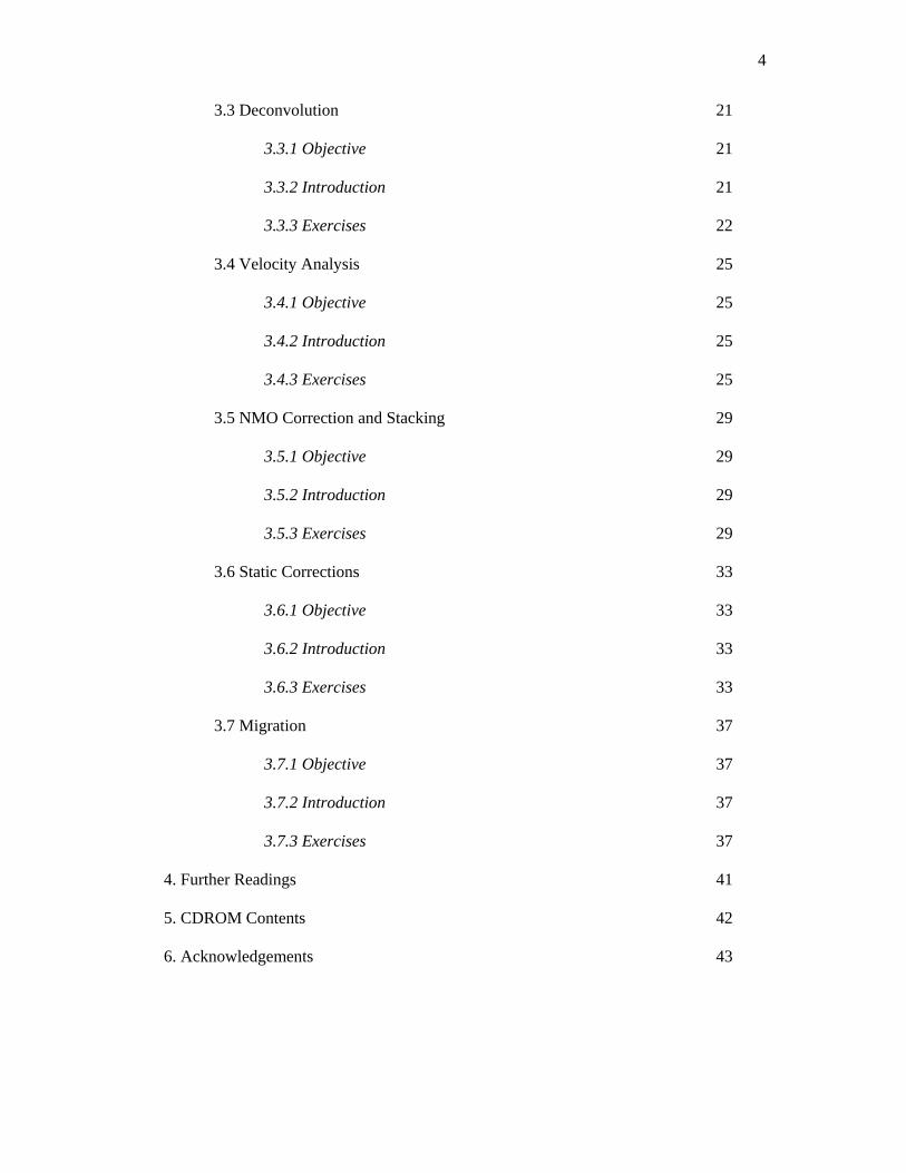
Table of Contents

Topic Page

1. Introduction 3

1.1 Seismic Data Processing 3

1.2 The Linux Operating System 5

1.3 The Seismic Unix Package 6

2. Installation 8

2.1 Linux OS 8

2.1.1 Hard-disk partitioning 8

2.1.2 Linux OS installation 9

2.2 SU Installation 10

3. Seismic Data Processing Tutorial 13

3.1 Preprocessing and data manipulation 13

3.1.1 Objective 13

3.1.2 Introduction 13

3.1.3 Information about the dataset 14

3.1.4 Exercises 14

3.2 Ground-roll Filtering 18

3.2.1 Objective 18


3.2.3 Exercises 18

4

3.3 Deconvolution 21

3.3.1 Objective 21


3.3.3 Exercises 22

3.4 Velocity Analysis 25

3.4.1 Objective 25


3.4.3 Exercises 25

3.5 NMO Correction and Stacking 29

3.5.1 Objective 29


3.5.3 Exercises 29

3.6 Static Corrections 33

3.6.1 Objective 33


3.6.3 Exercises 33

3.7 Migration 37

3.7.1 Objective 37


3.7.3 Exercises 37

4. Further Readings 41

5. CDROM Contents 42

6. Acknowledgements 43

5

1. Introduction

1.1 Seismic Data Processing

• The main objectives of seismic data processing are:

Improving the seismic resolution.

Increasing the S/N ratio.

• There are three primary stages in processing seismic data. In their usual order of

application, they are:

Deconvolution: It increases the vertical (time) resolution.

Stacking: It increases the S/N ratio.

Migration: It increases the horizontal resolution.

• Secondary processes are implemented at certain stages to condition the data and

improve the performance of these three processes.

• A typical seismic data processing flow includes the following steps:

1. Preprocessing involves the following processes (Yilmaz, 2001):

Demultiplexing: The data is transposed from the recording mode (each record

contains the same time sample from all traces) to the trace mode (each record

contains all time samples from one trace).

Reformatting: The data is converted into a convenient format that is used

throughout processing (e.g., SU and SEG-Y formats).

Trace editing: Bad traces, or parts of traces, are muted (zeroed) or killed (deleted)

from the data and polarity problems are fixed.

Gain application: Corrections are applied to account for amplitude loss due to

spherical divergence and absorption.

6

Setup of field geometry: The geometry of the field is written into the data (trace

headers) in order to associate each trace with its respective shot, offset, channel,

and CDP.

Application of field statics: In land surveys, elevation statics are applied to bring

the traveltimes to a common datum level.

(1) Deconvolution is performed along the time axis to increase vertical resolution by

compressing the basic seismic wavelet to approximately a spike and attenuating

multiples.

(2) CDP sorting transforms the data from shot-receiver (shot gather) to depth point-offset

(CDP gather) coordinates using the field geometry information.

4. Velocity analysis is performed on selected CDP gathers to estimate the stacking,

RMS, or NMO velocities to each reflector. Velocities are interpolated between the

analyzed CDPs.

5. Residual statics correction is usually needed for most land data. It corrects for

variations in the lateral velocity and thickness of the weathering layer.

6. NMO correction and muting: The stacking velocities are used to flatten the

reflections in each CDP gather (NMO correction). Muting zeros out the parts of

NMO-corrected traces that have been excessively stretched due to NMO correction.

7. Stacking: The NMO-corrected and muted traces in each CDP gather are summed

over the offset (stacked) to produce a single trace. Stacking M traces in a CDP

increases the S/N ratio of this CDP by M .

8. Poststack processing includes time-variant band-pass filtering, dip filtering, and other

processes to enhance the stacked section.

9. Migration: Dipping reflections are moved to their true subsurface positions and

diffractions are collapsed by migrating the stacked section.

7

1.2 The Linux Operating System

Linux is an operating system (OS) that was initially created as a hobby by a

young student, Linus Torvalds, at the University of Helsinki in Finland. He began his

work in 1991 when he released version 0.02 and worked steadily until 1994 when version

1.0 of the Linux Kernel was released. The kernel, at the heart of all Linux systems, is

developed and released under the GNU General Public License and its source code is

freely available to everyone. It is this kernel that forms the base around which a Linux

operating system is developed. There are now literally hundreds of companies and

organizations and an equal number of individuals that have released their own versions of

operating systems based on the Linux kernel. More information on the kernel can be

found at LinuxHQ and at the official Linux Kernel Archives.

Apart from the fact that it's freely distributed, Linux's functionality, adaptability

and robustness, has made it the main alternative for proprietary Unix and Microsoft

operating systems. IBM, Hewlett-Packard and other giants of the computing world have

embraced Linux and support its ongoing development. Well into its second decade of

existence, Linux has been adopted worldwide primarily as a server platform. Its use as a

home and office desktop operating system is also on the rise. The operating system can

also be incorporated directly into microchips in a process called "embedding" and is

increasingly being used this way in appliances and devices.

Throughout most of the 1990's, Linux was dismissed as a computer hobbyist

project, unsuitable for the general public's computing needs. Through the efforts of

developers of desktop management systems such as KDE and GNOME, office suite

project OpenOffice.org and the Mozilla web browser project, to name only a few, there

are now a wide range of applications that run on Linux and it can be used by anyone

8

regardless of his/her knowledge of computers. Those curious to see the capabilities of

Linux can download a live CD version called Knoppix . It comes with everything you

might need to carry out day-to-day tasks on the computer and it needs no installation. It

will run from a CD in a computer capable of booting from the CD drive. Those choosing

to continue using Linux can find a variety of versions or "distributions" of Linux that are

easy to install, configure and use. Information on these products is available at

www.linux.org/dist/index.html (www.linux.org, 2007).

1.3 The Seismic Unix Package

Seismic Unix (SU) package is a free software developed and maintained by the

Center for Wave Phenomena (CWP) at Colorado School of Mines. The package is

maintained and expanded periodically, with each new release appearing at 3 to 6 month

intervals, depending on changes that accumulate in the official version here at CWP. The

package is distributed with the full source code, so that users can alter and extend its

capabilities. The philosophy behind the package is to provide both a free processing and

development environment in a proven structure that can be maintained and expanded to

suit the needs of a variety of users.

The package is not necessarily restricted to seismic processing tasks, however. A

broad suite of wave-related processing can be done with SU, making it a somewhat more

general package than the word ``seismic'' implies. SU is intended as an extension of the

Unix operating system, and therefore shares many characteristics of the Unix, including

Unix flexibility and expandability. The fundamental Unix philosophy is that all operating

system commands are programs run under that operating system. The idea is that

individual tasks be identified, and that small programs be written to do those tasks, and

9

those tasks alone. The commands may have options that permit variations on those tasks,

but the fundamental idea is one-program, one-task. Because Unix is a multi-tasking

operating system, multiple processes may be strung together in a cascade via ``pipes'' (|).

This decentralization has the advantage of minimizing overhead by not launching

single ``monster'' applications that try to do everything, as is seen in Microsoft

applications, or in some commercial seismic utilities, for example. Unix has the added

feature of supporting a variety of shell languages, making Unix, itself, a meta-language.

Seismic Unix benefits from all of these attributes as well. In combination with standard

Unix programs, Seismic Unix programs may be used in shell scripts to extend the

functionality of the package. Of course, it may be that no Unix or Seismic Unix program

will fulfill a specific task. This means that new code has to be written. The availability of

a standard set of source code, designed to be readable by human beings, can expedite the

process of extending the package through the addition of new source code

(www.cwp.mines.edu, 2007).

10

2. Installation

2.1 Linux OS

• This part will explain how to install the Linux OS.

• The version that we will use is Redhat 10.0 (Fedora 1).

• The installation process includes basically the following two steps:

1. Hard-disk partitioning

2. Linux OS installation

2.1.1 Hard-disk partitioning

• This step is important because the Linux OS will not install on a Windows-formatted

hard disk partition (i.e., FAT, FAT32, or NTFS) .

• The most widely used software for partitioning is Partition Magic by PowerQuest,

which can be downloaded by KFUPM students from soft.kfupm.edu.sa (also included

in this CD).

• Follow the following steps for partitioning your PC hard disk:

1. Install Partition Magic on your PC.

2. Resize your hard disk to free about 15 GB of space.

3. Create the following logical Linux partitions in the newly-created free space:

One EXT2 partition for the OS with 5 GB size

One EXT2 partition for the data with 9 GB size.

One Linux Swap partition with 1 GB size (or equal to twice the size of

your PC RAM).

11

4. Apply the changes to your system and reboot the computer.

2.1.2 Linux OS installation

• Follow the following steps for installing the Redhat Linux OS on your PC hard disk:

1. Insert CD 1 into your CDROM drive and reboot your system from the CDROM.

2. Follow instructions until you reach the installation type step where you should

choose Standalone Development Workstation.

3. Follow instructions until you reach the partitioning step, where you should do the

following:

o Do not re-partition the hard disk using the Linux partition utility.

o Mount the 5-GB partition as “/”.

o Mount the 9-GB partition as “/home”.

4. Follow instructions until you reach the network setup step, where you should skip

it.

5. Follow instructions until you reach the Linux loader step, where you should do

the following:

o Use LILO as the OS loader.

o Make Windows the default OS.

o Create a Startup disk (if you like).

6. Follow instructions until you reach the root password step, where you should

enter the root password of your choice (to be used for Linux OS administration).

7. Follow instructions until you reach the Add Users step, where you should create

the username “seismic” and select a password for this account.

8. Follow instructions until installation ends, remove any disks, and restart the PC.

9. When the PC restarts and prompts you to select the OS, select Linux.

12

• More details on Redhat Linux installation can be found in the file Redhat-Linux-

Installation-Guide.pdf in this CD.

2.2 SU Installation

• Follow the following steps for installing SU under the Linux OS of your PC:

o Choose the KDE session as your desktop.

o Login as “seismic” (not root!).

o Open Konqueror by following: Start > Internet > Konqueror.

o Navigate to the directory “/home/seismic”.

o Make a directory called “su” within the directory “/home/seismic” by right-

clicking in an empty area of the files panel within Konqueror.

o Use Konqueror to navigate to the “/home/seismic” directory.

o In Konqueror, go to View and select “Show Hidden Files”.

o Right-click on the file called “.bash_profile” and Rename it to

“.bash_profile_original”.

o Copy the file “.bash_profile” in this CD to the directory “/home/seismic”.

o Re-login as user.

o Open Konqueror and download the current version (version 40 in this case) of SU

using the following steps:

o Type the following address into the address line of Konqueror:

ftp://ftp.cwp.mines.edu/pub/cwpcodes/

o Use your KFUPM internet proxy, account, and password.

o Download the file: cwp_su_all_40.tgz and save it in the “/home/seismic/su”

directory.

13

o Open a terminal by right-click on an empty area in the screen and selecting

“Konsole”.

o Within the terminal, go to the “/home/seismic/su” directory using the command:

cd /home/seismic/su

o Uncompress and untar the file cwp_su_all_40.tgz using the command:

zcat cwp_su_all_40.tgz | tar –xvf –

o Go to the “/home/seismic/su/src” directory using the command:

cd /home/seismic/su/src

o Within Konqueror, right-click on the file called “Makefile.config” and Rename it

to “Makefile.config.original”.

o Copy the file “Makefile.config” in this CD to the directory

“/home/seismic/su/src”.

o Compile the codes using the following command sequence (making sure that you

finish executing a command before you try the one after it!):

make install make xtinstall make finstall make utils

make xminstall make mglinstall

o A screen dump of a successful SU installation on Redhat Linux OS is given in

the file “install.successful” in this CD.

o As a test, type the following command in a terminal:

suascii

You should see the following output:

SUASCII – print non zero header values and data suascii <stdin >ascii_file Optional parameter: bare=0 print headers and data bare=1 print only data

14

bare=2 print headers only Notes: suwind/suus provide trace selection and/or subsampling. with bare=1 traces are separated by a blank line. Credits: CWP: Jack Trace header field accessed: ns

15

3. Seismic Data Processing Tutorial

• In this section, we will process a real seismic line called data.sgy (found in this CD)

from raw SEGY shot gathers to fully processed and stacked line.

• For the sake of organization, do the following:

1. Use Konqueror to navigate to the “/home/seismic” directory.

2. Create a directory called “tutorials” within the “/home/seismic” directory.

3. Open a terminal (Konsole) and type:

cd /home/seismic/tutorials

4. Copy the seismic data file data.sgy into the directory “/home/seismic/tutorials”.

• You must do all the tutorials while you are in a terminal and within the directory

“/home/seismic/tutorials” because the input data file and all outputs will be saved in

this directory.

3.1 Preprocessing and data manipulation

3.1.1 Objective

The objective of this tutorial is to get acquainted with the processing software

(Seismic Unix) and preprocess the dataset.

3.1.2 Introduction

Preprocessing involves the following steps:

(1) Demultiplexing.

16

(2) Reformatting.

(3) Editing.

(4) Geometrical spreading correction.

(5) Setup of field geometry.

(6) Application of field statics.

3.1.3 Information about the dataset

• Seismic data file name = data.sgy

• Sampling rate = 2 ms

• Number of samples/trace = 1501 samples

• Receiver spacing = 220 ft (66.7 m)

• Traces/shot (record) = 33

• Number of shots (records) = 18

• Number of traces in line = 594

3.1.4 Exercises

(1) The data has been demultiplexed already.

(2) The input data file data.sgy is in SEGY format and we want to reformat it to SU.

o Use the following command to convert the data from SEGY to SU format:

segyread tape=data.sgy verbose=1 endian=0 | segyclean > data.su

o Successful execution of this command should produce three files: data.su that

contains the seismic traces, binary that contains some binary information, and

header that contains header information about the line.

17

o Use the following command to view the first 6 shot records of the data (Figure 1):

suwind < data.su key=ep min=1 max=6 | suxwigb

o The xwigb window shows the traces with trace numbers along the horizontal axis

and the time (in seconds) along the vertical axis.

o Kill the xwigb window by clicking anywhere in it and pressing the letter “q” on

the keyboard.

(3) This dataset does not need editing.

(4) There are two ways to gain the dataset.

o Automatic Gain Control (AGC): Use the following command to gain the data

using the AGC method:

sugain < data.su agc=1 wagc=0.5 > data-agc.su

o Use the following command to view the result (Figure 2A):

suwind < data-agc.su key=ep min=1 max=6 | suxwigb

o t2: Use the following command to gain the data using the t2 method:

sugain < data.su agc=0 tpow=2.0 qclip=0.95 qbal=1 > data-tm.su

o Use the following command to view the result (Figure 2B):

suwind < data-tm.su key=ep min=1 max=6 | suxwigb

(5) The geometry is already setup.

(6) We will apply the field statics later.

18

Figure 1: Raw first 6 shot records.

Figure 2A: First 6 shot records after AGC.

19

Figure 2B: First 6 shot records after t2 gain.

20

3.2 Ground-roll Filtering

3.2.1 Objective

The objective of this tutorial is to use frequency filtering to filter out the ground

roll noise from the dataset.

3.2.2 Introduction

Frequency filtering involves the following steps:

(1) Taking the Fourier Transform (FT) of the data and displaying the amplitude spectrum

of the data to select the filter parameters.

(2) Filter application.

3.2.3 Exercises

(1) Take the FT of the data and save the amplitude spectrum using the command:

suspecfx < data-tm.su > data-tm-as.su

o Use the following command to view the result (Figure 3A):

suwind < data-tm-as.su key=ep min=1 max=6 | suxwigb

o To zoom within the xwigb panel, left-click and drag on your zoom area (Figure

3B).

(2) Use the following command to filter and save the data:

sufilter < data-tm.su f=15,20,50,60 > data-tm-flt.su

o Use the following command to view the result (Figure 4):

21

suwind < data-tm-flt.su key=ep min=1 max=6 | suxwigb

Figure 3A: Amplitude spectra of first 6 shot records, where the vertical axis indicates

frequency (Hz).

22

Figure 3B: Zoomed area of Figure 3A.

Figure 4: First 6 shot records after filtering.

23

3.3 Deconvolution

3.3.1 Objective

The objective of this tutorial is to deconvolve the dataset in order to spike it and

increase its vertical resolution.

3.3.2 Introduction

Deconvolution is used for two main purposes:

(1) Spiking the data to enhance the vertical resolution.

(2) Removing multiples from the data.

These two processes can be done by selecting appropriate values for the following

parameters:

o autocorrelation window (w)

o prediction lag (α)

o operator length (n)

o percent prewhitening (ε)

To achieve good results on deconvolution, we must perform the following processe in

sequence:

(1) Autocorrelation, which allows us to select the deconvolution type and related

parameters.

(2) Deconvolution.

(3) Gain to balance the amplitudes after deconvolution.

24

3.3.3 Exercises

(1) Autocorrelation:

o Use the following command to generate and save the trace autocorrelations:

suacor < data-tm-flt.su ntout=1001 sym=0 > data-tm-flt-ac.su


suwind < data-tm-flt-ac.su key=ep min=1 max=6 | suxwigb

o Examine the autocorrelations for the existence of long-path or short-path

multiples. Do you see evidence of any? (Answer: No!).

(2) Deconvolution:

o Use the following command to spike-deconvolve the data.

supef < data-tm-flt.su > data-tm-flt-dec.su minlag=0.002 maxlag=0.2

pnoise=0.001 mincorr=0 maxcorr=3


suwind < data-tm-flt-dec.su key=ep min=1 max=6 | suxwigb

o We used the following parameter values:

minlag=0.002 s, which sets the prediction lag parameter (α) for spiking

decocvolution.

maxlag=0.2 s, sets the operator length parameter (n) to the first transient

zone.

pnoise=0.001, which sets the percent prewhitening parameter (ε) to 0.1%

of the zero-lag autocorrelation value.

mincorr=0 s and maxcorr=3 s, which set the autocorrelation window

parameter (w) to the whole record.

25

(3) Gain:

o There might be unwanted scaling appearing in the data after deconvolution.

o It is convenient to apply a gain correction to re-scale the amplitudes using the

following command:

sugain < data-tm-flt-dec.su > data-tm-flt-dec-bal.su qbal=1 qclip=0.95


suwind < data-tm-flt-dec-bal.su key=ep min=1 max=6 | suxwigb

Figure 5: Autocorrelations of the first 6 shot records.

26

Figure 6: First 6 shot records after deconvolution.

Figure 7: First 6 shot records after deconvolution and amplitude balancing.

27

3.4 Velocity Analysis

3.4.1 Objective

The objective of this tutorial is to determine the stacking velocities in the data

area.

3.4.2 Introduction

Velocity analysis is used to determine the stacking velocity function along the

seismic line. The stacking velocities are then used in various seismic processing and

interpretation stages. Our main objective for determining the stacking velocities is to use

them for NMO correction. The stacking velocities can be determined using the constant-

velocity stack (CVS) or velocity spectrum methods. In this tutorial, we will use the

velocity spectrum method. Velocity analysis is performed on selected common depth

points (CDPs); therefore, we must sort the data from shot to CDP gathers before velocity

analysis.

3.4.3 Exercises

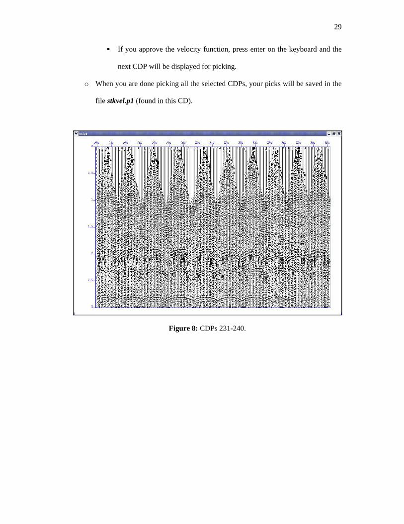
(1) CDP Sorting:

o Sort your data set processed so far data-tm-flt-dec-bal.su in cdp-offset domain

and save the CDP-sorted dataset using the following command:

susort < data-tm-flt-dec-bal.su > data-tm-flt-dec-bal-cdp.su cdp offset

o Use the following command to view CDPs 231-240 (Figure 8):

28

suwind < data-tm-flt-dec-bal-cdp.su key=cdp min=231 max=240 | suxwigb

(2) Velocity Analysis:

o Use Konqueror to copy the example shell script Velan from the directory

“/home/seismic/su/src/su/examples” to the directory “/home/seismic/tutorials”.

o Within Konqueror, right-click on Velan and select Open with KWrite.

o Within KWrite, ONLY change the following parameters in Velan:

velpanel=/home/seismic/tutorials/data-tm-flt-dec-bal-cdp.su

velpicks=/home/seismic/tutorials/stkvel.p1

nv=51, dv=200, fv=5000

cdpmin=225, cdpmax=250, dcdp=5

f1=15, f2=20, f3=50, f4=60

o Save the modified Velan script, exit KWrite, and open a terminal.

o Within the “/home/seismic/tutorials” directory, type the following command to

run the modified Velan script:

./Velan

o The velocity spectrum of CDP 225 will be displayed (Figure 9). Note that dark

areas in the velocity spectrum panel indicate higher semblance value.

Make your picks by pointing the mouse to your selected pick position and

typing “s” using the keyboard (remember that velocities for this dataset

are given in ft/sec although they are displayed as m/sec).

Continue picking until you are done with this CDP.

Type “q” using the keyboard to end picking for this CDP.

The velocity function for this CDP will be displayed for your approval.

29

If you approve the velocity function, press enter on the keyboard and the

next CDP will be displayed for picking.

o When you are done picking all the selected CDPs, your picks will be saved in the

file stkvel.p1 (found in this CD).

Figure 8: CDPs 231-240.

30

Figure 9: Velocity analysis of CDP 225.

31

3.5 NMO Correction and Stacking

3.5.1 Objective

The objective of this tutorial is to NMO-correct and stack the dataset.

3.5.2 Introduction

In this tutorial, we will use the sunmo and sustack commands to NMO-correct

the data and stack the traces in every CDP to produce the stacked section. The stacked

section gives an image of the subsurface in T0-CDP domain. It is used for later

processing and interpretation.

3.5.3 Exercises

(1) NMO Correction:

o Start with your dataset processed so far data-tm-flt-dec-bal-cdp.su.

o Use the following command to NMO-correct the dataset (note that we used the

velocity function that we got from the velocity analysis by copying it from the file

stkvel.p1):

sunmo < data-tm-flt-dec-bal-cdp.su > data-tm-flt-dec-bal-cdp-nmo.su

cdp=225,230,235,240,245,250

tnmo=0.0783034,0.337684,0.924959,1.31158,1.64927,1.75204,1.96248,2.60848

,2.8385

vnmo=5325.58,5813.95,7046.51,7790.7,8488.37,8976.74,9953.49,12000,12790.

32

7 tnmo=0.0440457,0.303426,0.636215,1.25775,1.92333,2.30995,2.79445

vnmo=5255.81,5674.42,6418.6,7558.14,8069.77,9465.12,11558.1

tnmo=0.0880914,0.411093,0.734095,1.42414,1.9429,2.36378,2.71126,2.81892

vnmo=5232.56,5883.72,6232.56,7139.53,8720.93,10558.1,12116.3,12767.4

tnmo=0.0978793,0.601958,1.67374,1.93801,2.28548,2.53997,2.78467

vnmo=5348.84,6441.86,8000,8674.42,9860.47,11209.3,12372.1

tnmo=0.0636215,0.415987,0.817292,1.15008,1.58564,1.68842,1.9478,2.1925,2.

45188,2.62806,2.87765

vnmo=5232.56,6186.05,7046.51,7511.63,8093.02,8279.07,8744.19,9395.35,104

18.6,11186,12209.3

tnmo=0.0734095,0.293638,0.626427,0.969005,1.32137,1.69821,1.98206,2.3295

3,2.64274,2.83361

vnmo=5232.56,5744.19,6534.88,7232.56,8000,8651.16,9558.14,10744.2,11534.

9,12930.2

o Use this command to view CDPs 231-240 after NMO correction (Figure 10):

suwind < data-tm-flt-dec-bal-cdp-nmo.su key=cdp min=231 max=240 | suxwigb

o Display the NMO-corrected CDPs in T-X domain and take a look at them. If

your reflections are not horizontally aligned, try another velocity function until

the reflections are horizontally aligned for all CDPs and times (Hint: Our velocity

function is fine!).

(2) Stacking:

o Use this command to stack the NMO-corrected file:

sustack < data-tm-flt-dec-bal-cdp-nmo.su > data-tm-flt-dec-bal-cdp-nmo-

stack.su

o Use this command to view the stacked section (Figure 11):

33

suxwigb < data-tm-flt-dec-bal-cdp-nmo-stack.su

Figure 10: CDPs 231-240 after NMO correction.

34

Figure 11: Stacked section. Horizontal axis indicates CDP numbers.

35

3.6 Static Corrections

3.6.1 Objective

The objective of this tutorial is to apply field and residual static corrections on the

dataset.

3.6.2 Introduction

The filed static correction accounts for variable source and receiver elevations and

puts them all on a flat datum (reference elevation). The residual static correction

accounts for the lateral thickness and velocity variation in the weathering layer.

3.6.3 Exercises

(1) Field Static Correction:

o The command sustatic is used to apply any type of static shifts to the traces.

o In order to calculate the elevation static correction, the following information is

required for every trace:

(i) Source elevation from datum

(ii) Receiver elevation from datum

(iii)Weathering-layer velocities under the source and the receiver

(iv) Sub-weathering layer velocities under the source and the receiver

36

o Information (i) and (ii) are usually available for every survey and is available in

our dataset.

o Information (iii) and (iv) have to be estimated from uphole or refraction data. The

theory and application of these methods is beyond the scope of this manual.

o We will not apply the field correction to the data because the required velocities

are not available.

(2) Residual Static Correction:

o The command suresstat is used to calculate the residual static shift for every

source, receiver, and trace. It requires that the data be NMO-corrected and sorted

in shot gathers and offset within each shot gather.

o Use the following command to sort the NMO-corrected data into shot gathers:

susort < data-tm-flt-dec-bal-cdp-nmo.su > data-tm-flt-dec-bal-cdp-nmo-fldr.su

fldr offset

o Use this command to view the first 6 NMO-corrected shot records (Figure 12):

suwind < data-tm-flt-dec-bal-cdp-nmo-fldr.su key=ep min=1 max=6 | suxwigb

o Use the following command to calculate the residual static shift for every source

and receiver:

suresstat < data-tm-flt-dec-bal-cdp-nmo-fldr.su ssol=sstats rsol=rstats

ntraces=594 ntpick=50 niter=5 nshot=19 nr=33 nc=594 sfold=33 rfold=18

cfold=18

o Execution of the above suresstat command should produce two binary files

named sstats and rstats.

o The command sustatic is used then to apply these residual static shifts to the

traces.

37

o Use the following command to apply the source and receiver residual statics to

the traces:

sustatic < data-tm-flt-dec-bal-cdp-nmo.su > data-tm-flt-dec-bal-cdp-nmo-

stat.su hdrs=3 sou_file=sstats rec_file=rstats ns=19 nr=65

o Use this command to view CDPs 231-240 after NMO correction and residual

static correction (Figure 13):

suwind < data-tm-flt-dec-bal-cdp-nmo-stat.su key=cdp min=231 max=240 |

suxwigb

o We can see that the NMO-corrected reflections within these CDP gathers have

been more horizontally aligned after residual static correction (compare with

Figure 10).

Figure 12: First 6 shot records after NMO correction.

38

Figure 13: CDPs 231-240 after NMO and residual-static corrections.

39

3.7 Migration

3.7.1 Objective

The objective of this tutorial is to migrate the dataset.

3.7.2 Introduction

Seismic migration enhances the horizontal resolution by collapsing diffractions

and moving dipping reflectors to their true subsurface locations. There are several types

and algorithms of migration. We will use the Stolt (FK) migration algorithm on our 2D

poststack time section.

3.7.3 Exercises

o Use the following command to migrate the stacked time section (data-tm-flt-dec-bal-

cdp-nmo-stack.su) by Stolt migration:

sustolt < data-tm-flt-dec-bal-cdp-nmo-stack.su cdpmin=210 cdpmax=260

dxcdp=110 smig=0.6

tmig=0.0734095,0.293638,0.626427,0.969005,1.32137,1.69821,1.98206,2.3295

3,2.64274,2.83361

vmig=5232.56,5744.19,6534.88,7232.56,8000,8651.16,9558.14,10744.2,11534.

9,12930.2 | sugain qclip=0.98 > data-tm-flt-dec-bal-cdp-nmo-stack-mig.su

o Use this command to view the stacked migrated section (Figure 14):

suxwigb < data-tm-flt-dec-bal-cdp-nmo-stack-mig.su

40

o We can see that migration did not change the data considerably because of the flat

nature of reflections in the area where the data was acquired.

Figure 14: Stacked section after Stolt migration. Horizontal axis indicates CDP numbers.

41

4. Further Readings

Al-Shuhail, A. A., 2007. GEOP320 Course Notes:

http://faculty.kfupm.edu.sa/ES/ashuhail/GEOP320.htm.

Center for Wave Phenomena, 2007. Seismic Uni*x:

ftp://ftp.cwp.mines.edu/pub/cwpcodes/, (included in this CDROM

in the directory SU).

FreeUSP.org, 2007. Free USP Software Website: http://www.freeusp.org/.

Yilmaz, O., 2001. Seismic Data Analysis: SEG.

42

5. CDROM Contents

• The CDROM includes the following components:

1. This document.

2. Linux directory that includes the file Redhat-Linux-Installation-Guide.pdf, the

Redhat Linux OS installation instructions. A full copy of the latest version

Redhat Linux is not included in the CDROM due to its excessively large size but

can be bought or downloaded freely from Redhat website at:

https://www.redhat.com/apps/download/.

3. PM8p0 directory that includes the following components:

o Partition_Magic_8.0.zip: Partition Magic version 8.0 software

o PM8Quick.pdf: Quick installation manual of Partition Magic

o PM8.pdf: Extensive installation manual of Partition Magic

4. SU directory that includes the following components:

o .bash_profile: a file needed for SU installation

o cwp_su_all_40.tar: SU version 40 software

o Installation_Instructions.txt: SU installation instructions

o Makefile.config: a file needed for SU installation

o selfdocs_600dpi_a4.pdf: Full listings of all SU commands description

o sumanual_600dpi_a4.pdf: Extensive SU manual

5. Tutorials directory that includes all files required for the Tutorials explained in

part 3 of this document.

43

6. Acknowledgements

I would like to thank KFUPM for supporting this work through the 2007 Summer

Special Assignment program. I also thank the Center for Wave Phenomena at Colorado

School of Mines and its sponsors for creating and maintaining the SU package.

Seismic Unix Manual00

Documents

Transcript of Seismic Unix Manual00