Seismic Hazard Levels - onlinepubs.trb.org
91
TRB Webinar: Load and Resistance Factor Design Analysis for Seismic Design of Slopes and Retaining Walls
Transcript of Seismic Hazard Levels - onlinepubs.trb.org

TRB Webinar: Load and Resistance Factor Design
Analysis for Seismic Design of Slopes and Retaining Walls

TRB Announcements: We have emailed you the presenters’ slides in today’s webinar
reminder email.
Upcoming webinars: Practices for Roadway Tunnel Design, Construction, Safety and Inspection, and Rehabilitation: March 4, 2 PM EST
Nighttime Seat Belt Enforcement: Background and Recent Findings: March 9, 2 PM ESTMore: http://bit.ly/TRBwebinar
Follow TRB on Twitter @TRBofNAhttp://twitter.com/TRBofNA

Today’s Presenters and ModeratorMike Keever, California Department of Transportation, [email protected]
Edward Kavazanjian, Arizona State University, [email protected]
Donald Anderson, CH2MHill, [email protected]
Geoffrey Martin, University of Southern California, [email protected]

11
Load and Resistance Factor Designfor
Seismic Design of Slopes and Retaining Walls
sponsored by
TRB Committee AFF50Seismic Design of Bridges
February 17, 2010
TRB Webinar
22
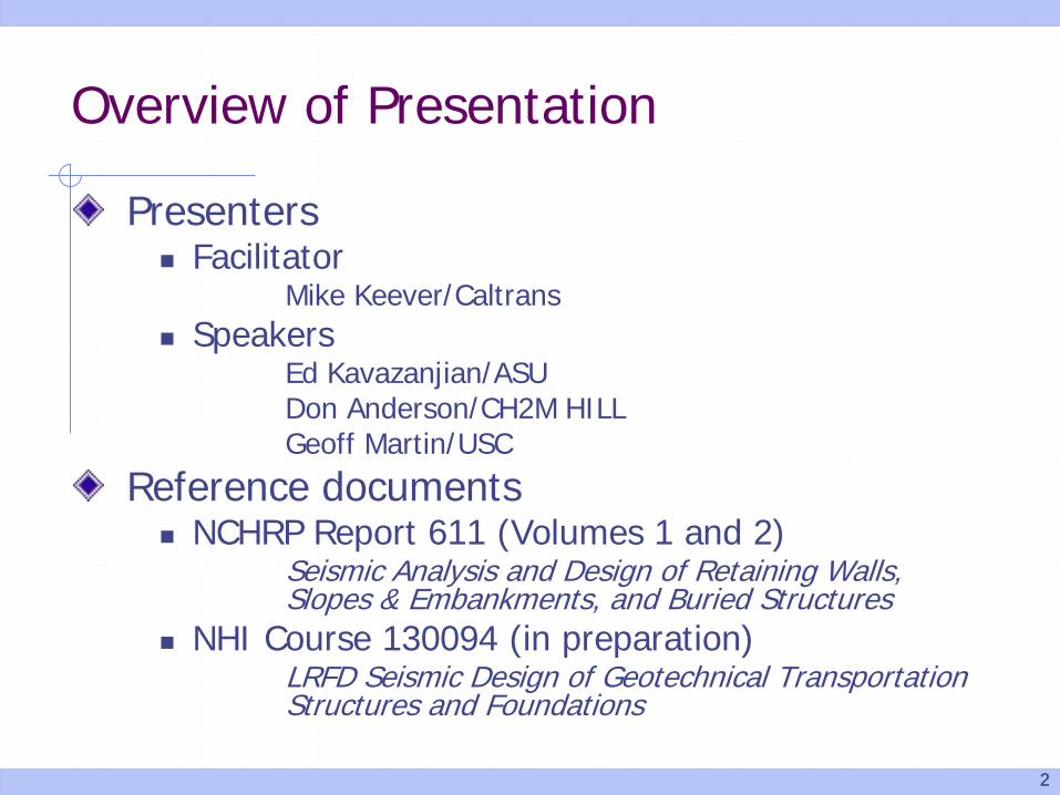
Overview of Presentation
Presenters Facilitator
Mike Keever/Caltrans Speakers
Ed Kavazanjian/ASUDon Anderson/CH2M HILL Geoff Martin/USC
Reference documents NCHRP Report 611 (Volumes 1 and 2)
Seismic Analysis and Design of Retaining Walls, Slopes & Embankments, and Buried Structures
NHI Course 130094 (in preparation)LRFD Seismic Design of Geotechnical Transportation Structures and Foundations
33
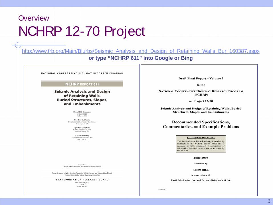
Overview
NCHRP 12-70 Projecthttp://www.trb.org/Main/Blurbs/Seismic_Analysis_and_Design_of_Retaining_Walls_Bur_160387.aspx
or type “NCHRP 611” into Google or Bing
44
Overview
Objectives of NCHRP 12-70 Project
Develop methods for LRFD seismic design of retaining walls, buried structures, slopes, and embankmentsDevelop recommended specifications compatible and consistent with AASHTO LRFD Bridge Design Specifications
Ref: NCHRP Research Project Statement Project 12-70, FY 2004
55
Overview
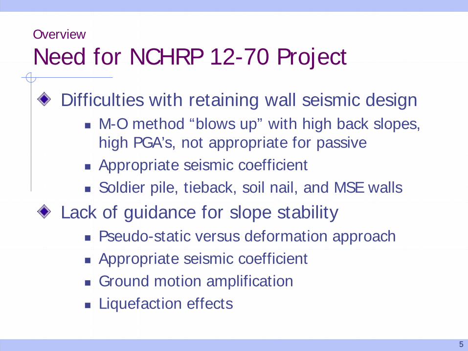
Need for NCHRP 12-70 Project
Difficulties with retaining wall seismic design M-O method “blows up” with high back slopes,
high PGA’s, not appropriate for passive Appropriate seismic coefficient Soldier pile, tieback, soil nail, and MSE walls
Lack of guidance for slope stability Pseudo-static versus deformation approach Appropriate seismic coefficient Ground motion amplification Liquefaction effects
66
Outline of Presentation
Background for methodology - Kavazanjian
Seismic slope stability - Anderson
Retaining wall design - Martin
77
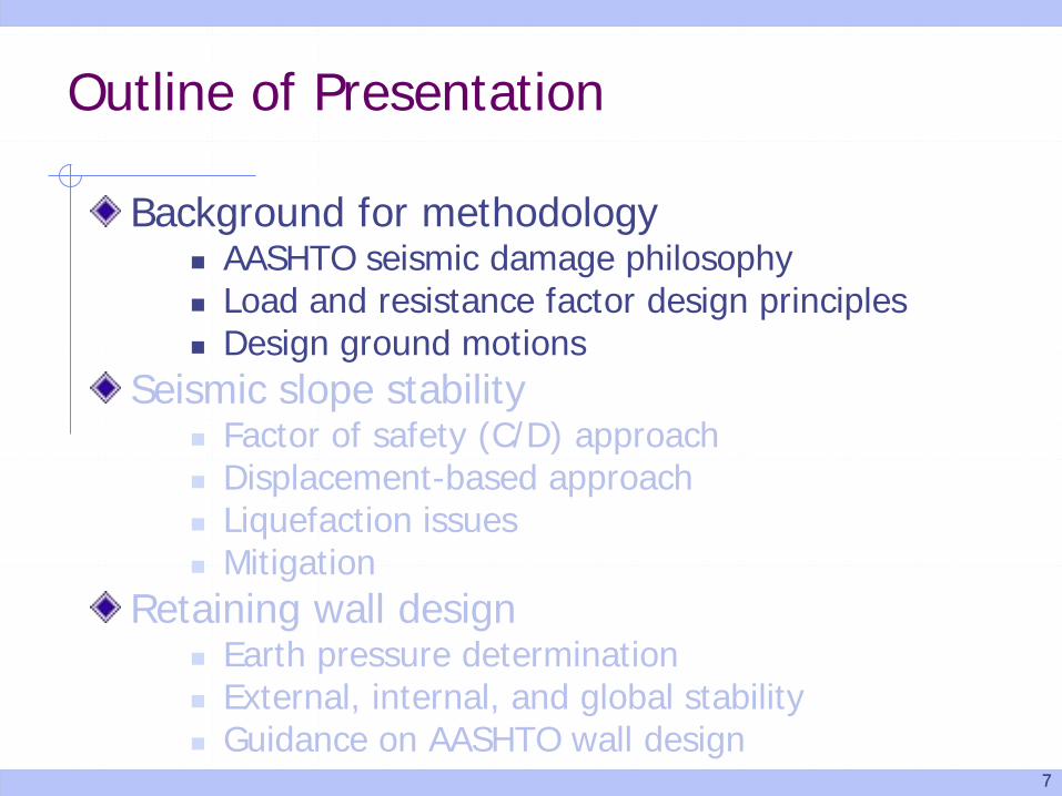
Outline of Presentation
Background for methodology AASHTO seismic damage philosophy Load and resistance factor design principles Design ground motions
Seismic slope stability Factor of safety (C/D) approach Displacement-based approach Liquefaction issues Mitigation
Retaining wall design Earth pressure determination External, internal, and global stability Guidance on AASHTO wall design
88
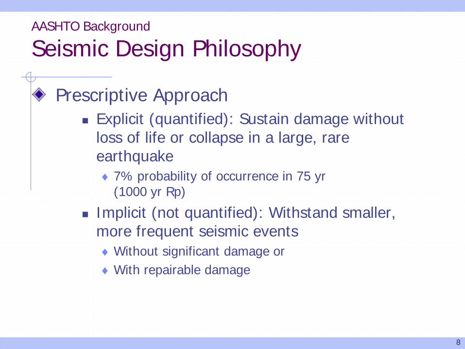
Prescriptive Approach Explicit (quantified): Sustain damage without
loss of life or collapse in a large, rare earthquake♦ 7% probability of occurrence in 75 yr
(1000 yr Rp)
Implicit (not quantified): Withstand smaller, more frequent seismic events♦ Without significant damage or ♦ With repairable damage
AASHTO Background
Seismic Design Philosophy
99
Alternative approaches (Owner’s discretion) More rigorous performance standard
♦ e.g., 3% probability of occurrence in 75 yr
Multi-level (performance-based) design standard♦ Upper level event for “No Collapse”♦ Lower level event for “No Damage”
Often applied to facilities of high importance♦ Critical bridges♦ Lifelines routes
AASHTO Background
Seismic Design Philosophy
1010
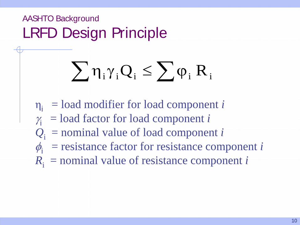
ηi = load modifier for load component iγi = load factor for load component iQi = nominal value of load component iφi = resistance factor for resistance component iRi = nominal value of resistance component i
∑∑ ϕ≤γη iiiii RQ
AASHTO Background
LRFD Design Principle
1111
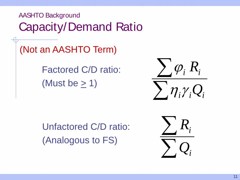
Factored C/D ratio:(Must be > 1)
Unfactored C/D ratio:(Analogous to FS) ∑
∑i
i
QR
∑∑
iii
ii
QR
γηϕ
AASHTO Background
Capacity/Demand Ratio
(Not an AASHTO Term)
1212
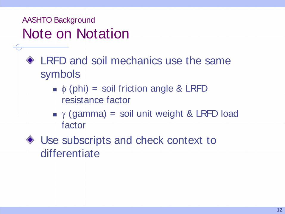
LRFD and soil mechanics use the same symbols
φ (phi) = soil friction angle & LRFD resistance factor
γ (gamma) = soil unit weight & LRFD load factor
Use subscripts and check context to differentiate
AASHTO Background
Note on Notation
1313
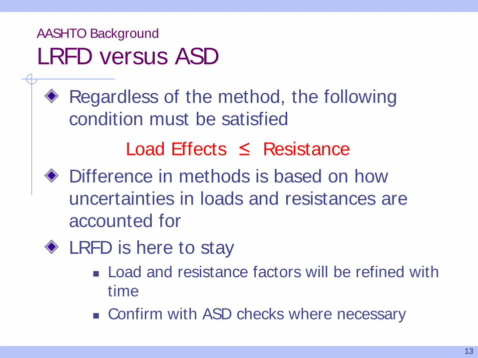
Regardless of the method, the following condition must be satisfied
Load Effects ≤ ResistanceDifference in methods is based on how uncertainties in loads and resistances are accounted forLRFD is here to stay
Load and resistance factors will be refined with time
Confirm with ASD checks where necessary
AASHTO Background
LRFD versus ASD
1414
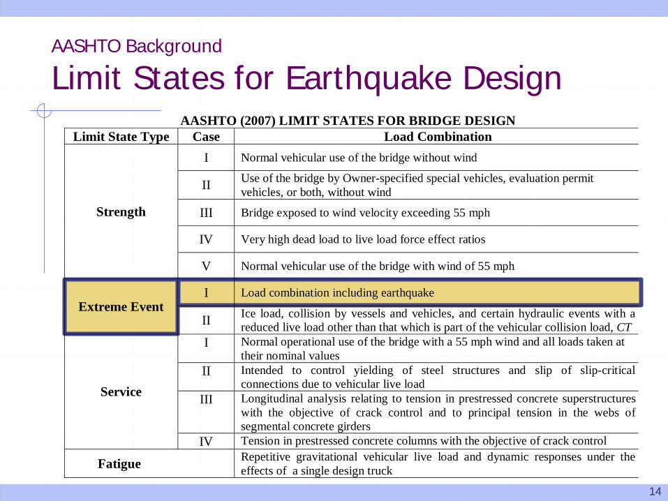
AASHTO (2007) LIMIT STATES FOR BRIDGE DESIGN Limit State Type Case Load Combination
I Normal vehicular use of the bridge without wind
II Use of the bridge by Owner-specified special vehicles, evaluation permit vehicles, or both, without wind
III Bridge exposed to wind velocity exceeding 55 mph
IV Very high dead load to live load force effect ratios
Strength
V Normal vehicular use of the bridge with wind of 55 mph
I Load combination including earthquake Extreme Event
II Ice load, collision by vessels and vehicles, and certain hydraulic events with a reduced live load other than that which is part of the vehicular collision load, CT
I Normal operational use of the bridge with a 55 mph wind and all loads taken at their nominal values
II Intended to control yielding of steel structures and slip of slip-critical connections due to vehicular live load
III Longitudinal analysis relating to tension in prestressed concrete superstructures with the objective of crack control and to principal tension in the webs of segmental concrete girders
Service
IV Tension in prestressed concrete columns with the objective of crack control
Fatigue Repetitive gravitational vehicular live load and dynamic responses under the effects of a single design truck
AASHTO Background
Limit States for Earthquake Design
1515
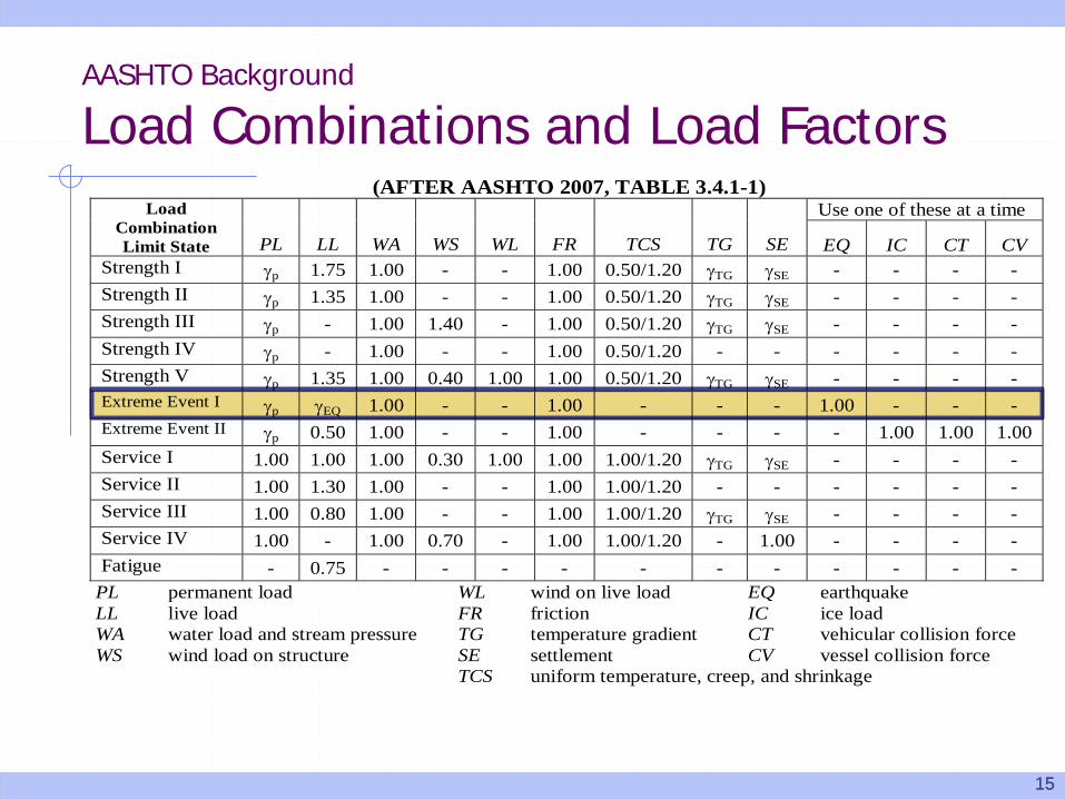
(AFTER AASHTO 2007, TABLE 3.4.1-1) Use one of these at a time Load
Combination Limit State PL LL WA WS WL FR TCS TG SE EQ IC CT CV
Strength I γp 1.75 1.00 - - 1.00 0.50/1.20 γTG γSE - - - - Strength II γp 1.35 1.00 - - 1.00 0.50/1.20 γTG γSE - - - - Strength III γp - 1.00 1.40 - 1.00 0.50/1.20 γTG γSE - - - - Strength IV γp - 1.00 - - 1.00 0.50/1.20 - - - - - - Strength V γp 1.35 1.00 0.40 1.00 1.00 0.50/1.20 γTG γSE - - - - Extreme Event I γp γEQ 1.00 - - 1.00 - - - 1.00 - - - Extreme Event II γp 0.50 1.00 - - 1.00 - - - - 1.00 1.00 1.00 Service I 1.00 1.00 1.00 0.30 1.00 1.00 1.00/1.20 γTG γSE - - - - Service II 1.00 1.30 1.00 - - 1.00 1.00/1.20 - - - - - - Service III 1.00 0.80 1.00 - - 1.00 1.00/1.20 γTG γSE - - - - Service IV 1.00 - 1.00 0.70 - 1.00 1.00/1.20 - 1.00 - - - - Fatigue - 0.75 - - - - - - - - - - -
PL permanent load WL wind on live load EQ earthquake LL live load FR friction IC ice load WA water load and stream pressure TG temperature gradient CT vehicular collision force WS wind load on structure SE settlement CV vessel collision force
TCS uniform temperature, creep, and shrinkage
AASHTO Background
Load Combinations and Load Factors
1616
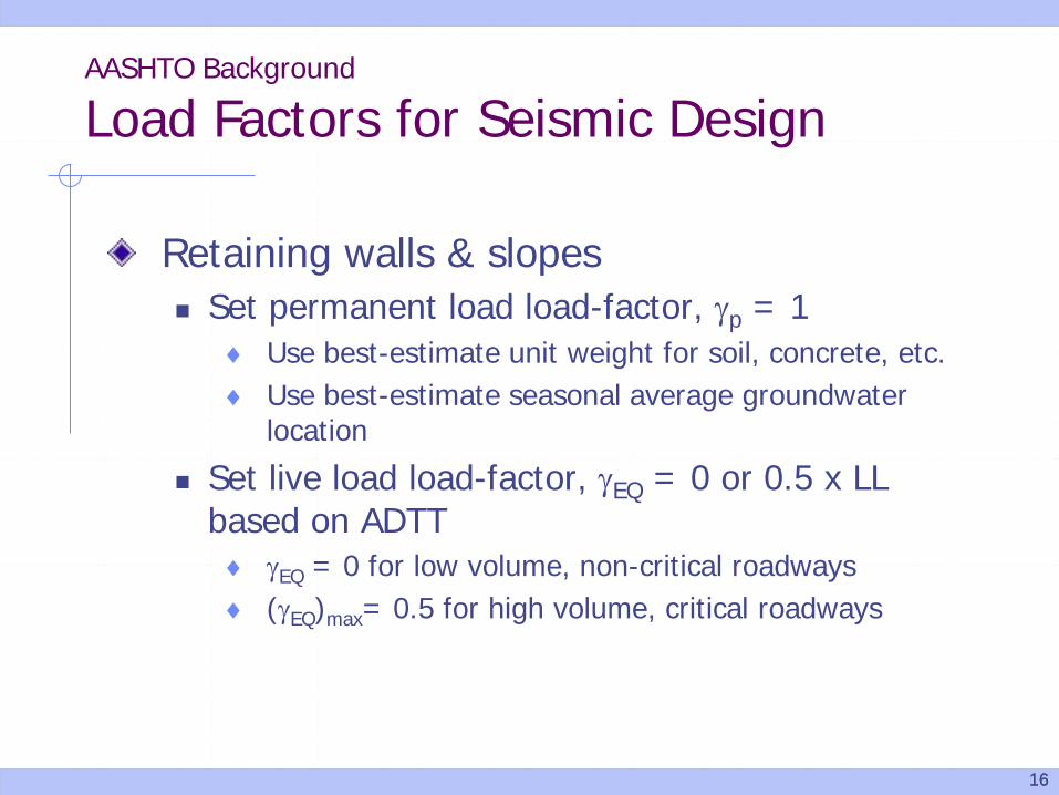
Retaining walls & slopes Set permanent load load-factor, γp = 1
♦ Use best-estimate unit weight for soil, concrete, etc.♦ Use best-estimate seasonal average groundwater
location
Set live load load-factor, γEQ = 0 or 0.5 x LL based on ADTT
♦ γEQ = 0 for low volume, non-critical roadways♦ (γEQ)max= 0.5 for high volume, critical roadways
AASHTO Background
Load Factors for Seismic Design
1717
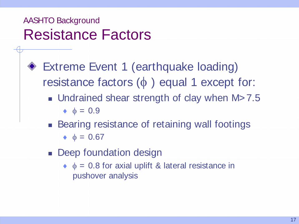
Extreme Event 1 (earthquake loading) resistance factors (φ ) equal 1 except for: Undrained shear strength of clay when M>7.5
♦ φ = 0.9
Bearing resistance of retaining wall footings♦ φ = 0.67
Deep foundation design♦ φ = 0.8 for axial uplift & lateral resistance in
pushover analysis
AASHTO Background
Resistance Factors
1818
AASHTO Background
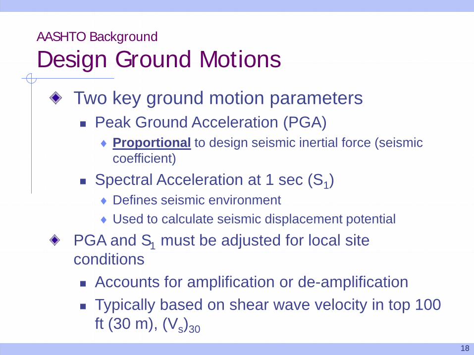
Design Ground Motions
Two key ground motion parameters Peak Ground Acceleration (PGA)
♦ Proportional to design seismic inertial force (seismic coefficient)
Spectral Acceleration at 1 sec (S1)♦ Defines seismic environment ♦ Used to calculate seismic displacement potential
PGA and S1 must be adjusted for local site conditions Accounts for amplification or de-amplification Typically based on shear wave velocity in top 100
ft (30 m), (Vs)30
1919
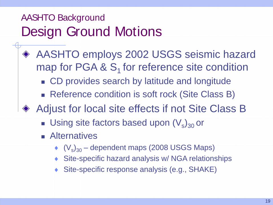
AASHTO Background
Design Ground Motions
AASHTO employs 2002 USGS seismic hazard map for PGA & S1 for reference site condition CD provides search by latitude and longitude Reference condition is soft rock (Site Class B)
Adjust for local site effects if not Site Class B Using site factors based upon (Vs)30 or Alternatives
♦ (Vs)30 – dependent maps (2008 USGS Maps)♦ Site-specific hazard analysis w/ NGA relationships♦ Site-specific response analysis (e.g., SHAKE)
2020
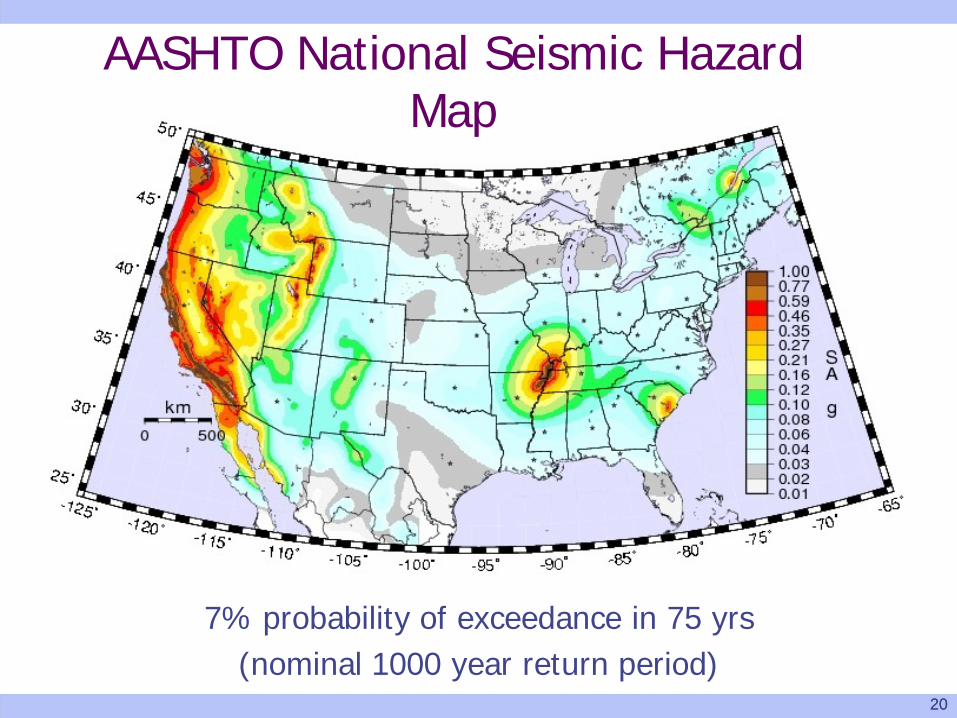
7% probability of exceedance in 75 yrs (nominal 1000 year return period)
AASHTO National Seismic Hazard Map
2121
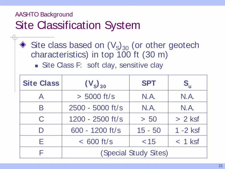
AASHTO Background
Site Classification System
Site class based on (VS)30 (or other geotech characteristics) in top 100 ft (30 m) Site Class F: soft clay, sensitive clay
Site Class (VS)30 SPT Su
A > 5000 ft/s N.A. N.A.B 2500 - 5000 ft/s N.A. N.A.C 1200 - 2500 ft/s > 50 > 2 ksfD 600 - 1200 ft/s 15 - 50 1 -2 ksfE < 600 ft/s <15 < 1 ksfF (Special Study Sites)
2222
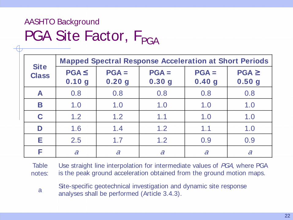
AASHTO Background
PGA Site Factor, FPGA
Site Class
Mapped Spectral Response Acceleration at Short Periods
PGA ≤ 0.10 g
PGA = 0.20 g
PGA = 0.30 g
PGA = 0.40 g
PGA ≥ 0.50 g
A 0.8 0.8 0.8 0.8 0.8
B 1.0 1.0 1.0 1.0 1.0
C 1.2 1.2 1.1 1.0 1.0
D 1.6 1.4 1.2 1.1 1.0
E 2.5 1.7 1.2 0.9 0.9
F a a a a a
Table notes:
Use straight line interpolation for intermediate values of PGA, where PGA is the peak ground acceleration obtained from the ground motion maps.
a Site-specific geotechnical investigation and dynamic site response analyses shall be performed (Article 3.4.3).
2323
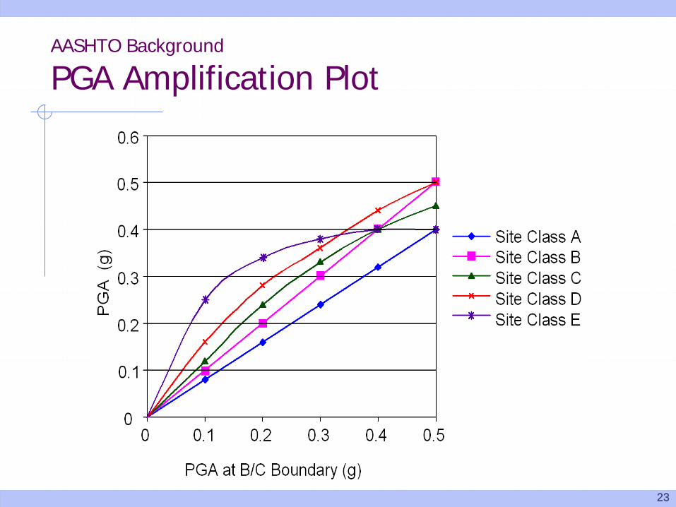
AASHTO Background
PGA Amplification Plot
2424
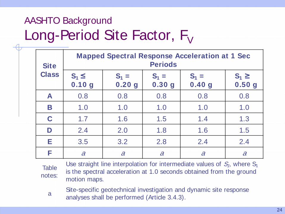
AASHTO Background
Long-Period Site Factor, FV
Site Class
Mapped Spectral Response Acceleration at 1 Sec Periods
S1 ≤ 0.10 g
S1 = 0.20 g
S1 = 0.30 g
S1 = 0.40 g
S1 ≥ 0.50 g
A 0.8 0.8 0.8 0.8 0.8
B 1.0 1.0 1.0 1.0 1.0
C 1.7 1.6 1.5 1.4 1.3
D 2.4 2.0 1.8 1.6 1.5
E 3.5 3.2 2.8 2.4 2.4
F a a a a a
Table notes:
Use straight line interpolation for intermediate values of S1, where S1
is the spectral acceleration at 1.0 seconds obtained from the ground motion maps.
a Site-specific geotechnical investigation and dynamic site response analyses shall be performed (Article 3.4.3).
25
Outline of Presentation
Background for methodology AASHTO seismic damage philosophy Load and resistance factor design principles Design ground motions
Seismic slope stability Factor of safety (C/D) approach Displacement-based approach Liquefaction issues Mitigation
Retaining wall design Earth pressure determination External, internal, and global stability Guidance on AASHTO walls
26
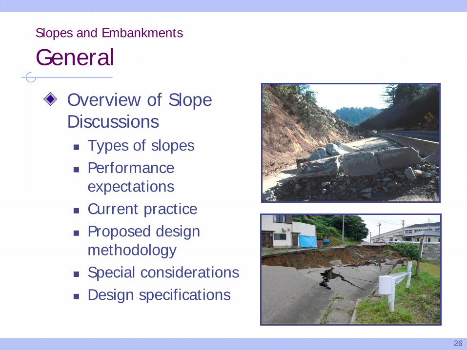
Overview of Slope Discussions Types of slopes Performance
expectations Current practice Proposed design
methodology Special considerations Design specifications
Slopes and Embankments
General
27
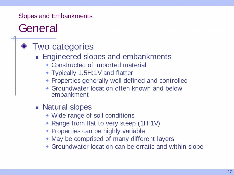
Slopes and Embankments
GeneralTwo categories Engineered slopes and embankments Constructed of imported material Typically 1.5H:1V and flatter Properties generally well defined and controlled Groundwater location often known and below
embankment
Natural slopes Wide range of soil conditions Range from flat to very steep (1H:1V) Properties can be highly variable May be comprised of many different layers Groundwater location can be erratic and within slope
28
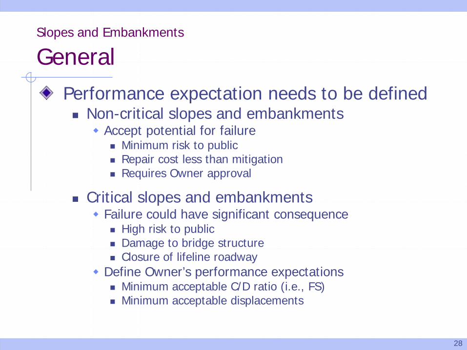
Performance expectation needs to be defined Non-critical slopes and embankments Accept potential for failure
Minimum risk to public Repair cost less than mitigation Requires Owner approval
Critical slopes and embankments Failure could have significant consequence
High risk to public Damage to bridge structure Closure of lifeline roadway
Define Owner’s performance expectations Minimum acceptable C/D ratio (i.e., FS) Minimum acceptable displacements
Slopes and Embankments
General
29
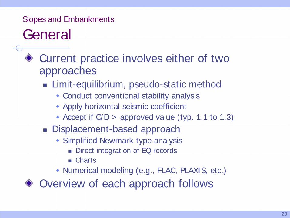
Current practice involves either of two approaches Limit-equilibrium, pseudo-static method Conduct conventional stability analysis Apply horizontal seismic coefficient Accept if C/D > approved value (typ. 1.1 to 1.3)
Displacement-based approach Simplified Newmark-type analysis
Direct integration of EQ records Charts
Numerical modeling (e.g., FLAC, PLAXIS, etc.)
Overview of each approach follows
Slopes and Embankments
General
30
Slopes and Embankments
Limit-Equilibrium Method
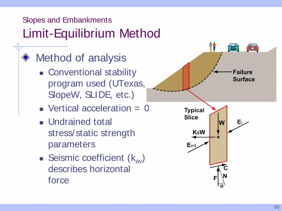
Method of analysis Conventional stability
program used (UTexas, SlopeW, SLIDE, etc.)
Vertical acceleration = 0 Undrained total
stress/static strength parameters
Seismic coefficient (kav) describes horizontal force
31
Slopes and Embankments
Limit-Equilibrium Method
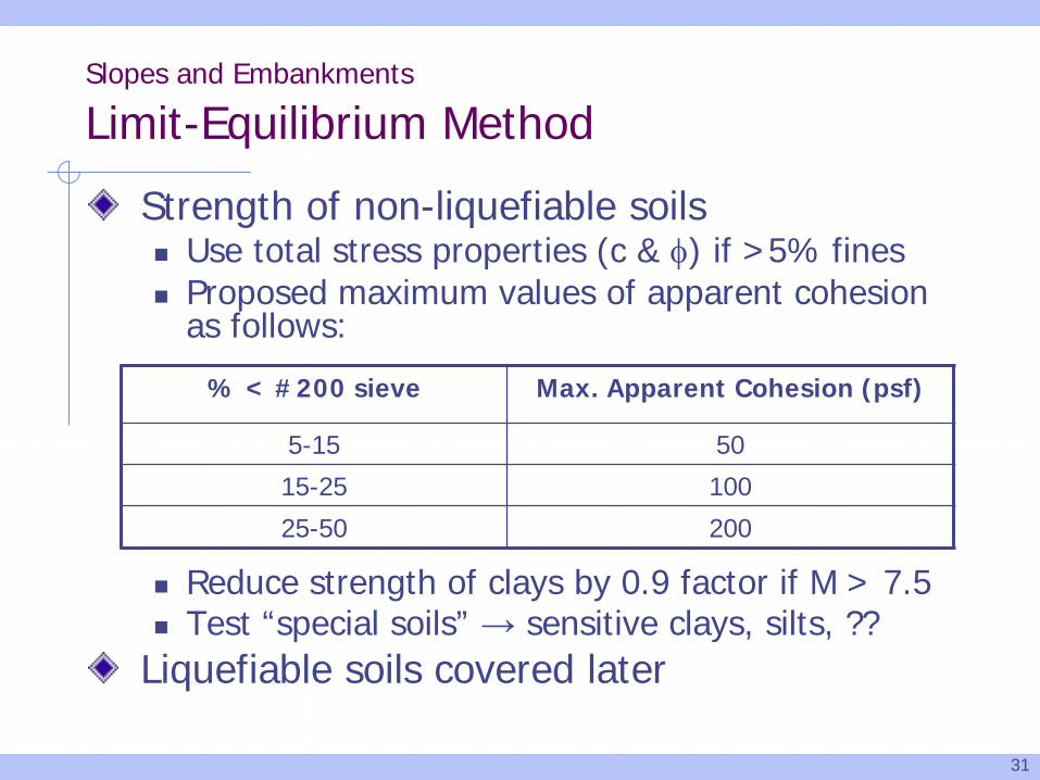
Strength of non-liquefiable soils Use total stress properties (c & φ) if >5% fines Proposed maximum values of apparent cohesion
as follows:
Reduce strength of clays by 0.9 factor if M > 7.5 Test “special soils” → sensitive clays, silts, ??
Liquefiable soils covered later
% < #200 sieve Max. Apparent Cohesion (psf)
5-15 50
15-25 100
25-50 200
32
Slopes and Embankments
Limit-Equilibrium Method
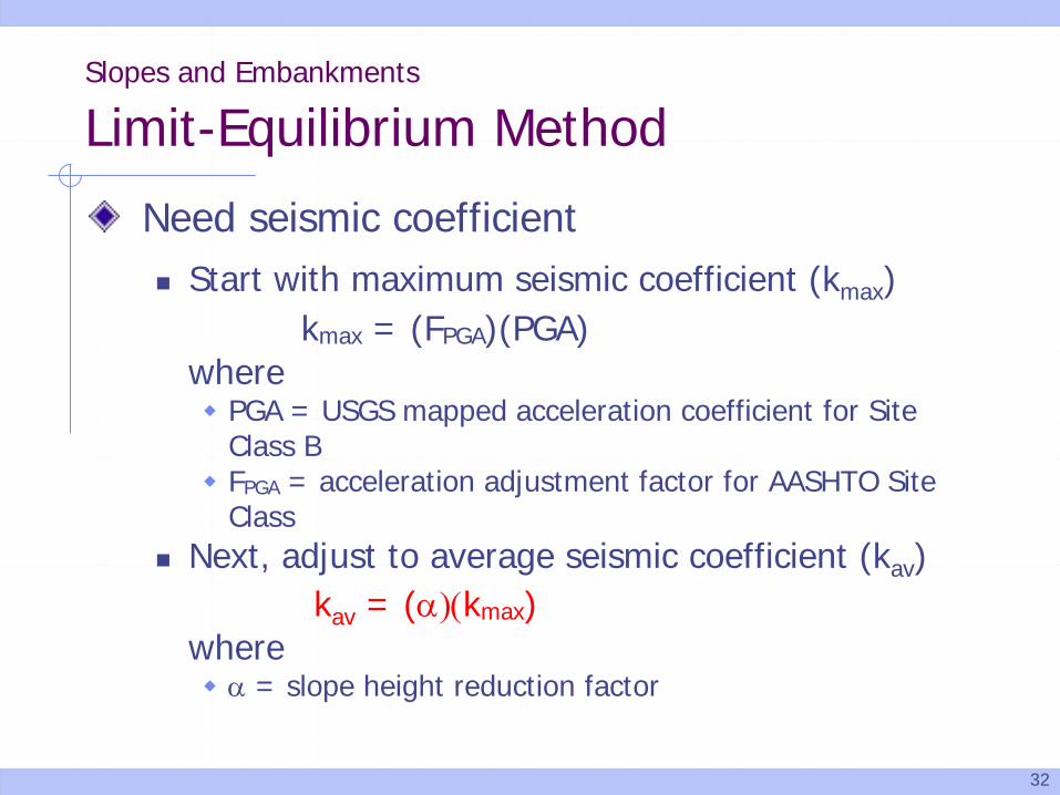
Need seismic coefficient Start with maximum seismic coefficient (kmax)
kmax = (FPGA)(PGA)where PGA = USGS mapped acceleration coefficient for Site
Class B FPGA = acceleration adjustment factor for AASHTO Site
Class Next, adjust to average seismic coefficient (kav)
kav = (α)(kmax)where α = slope height reduction factor
33
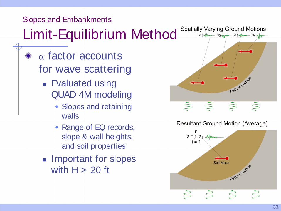
Slopes and Embankments
Limit-Equilibrium Methodα factor accounts for wave scattering Evaluated using
QUAD 4M modeling Slopes and retaining
walls Range of EQ records,
slope & wall heights, and soil properties
Important for slopes with H > 20 ft
34
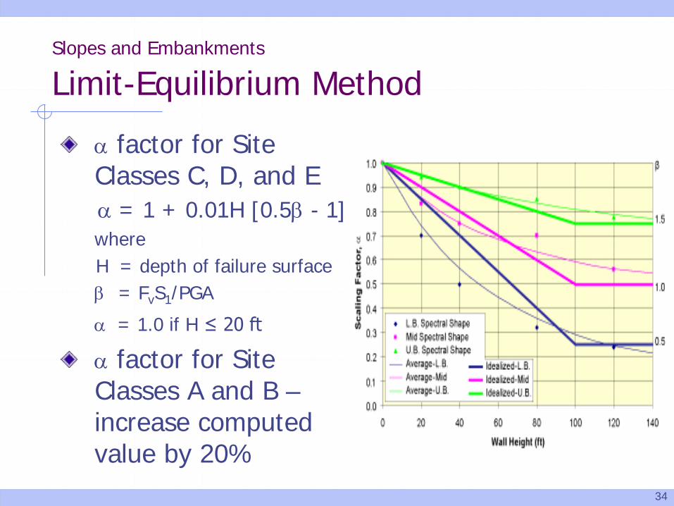
Slopes and Embankments
Limit-Equilibrium Method
α factor for Site Classes C, D, and Eα = 1 + 0.01H [0.5β - 1]whereH = depth of failure surface β = FvS1/PGA
α = 1.0 if H ≤ 20 ft
α factor for Site Classes A and B –increase computed value by 20%
35
Slopes and Embankments
Limit-Equilibrium Method
Next, apply displacement (ductility) factor, r kav = r α kmax
reduces kmax for allowable permanent displacement
Values of r = 1.0 to 0.5 For r =1.0, kav = α kmax
C/D (FS) > 1 – Negligibly small permanent displacement Very conservative design criteria
For r = 0.5, kav = 0.5 α kmax
C/D (FS) = 1.0 => 1–2 inches permanent displacement C/D (FS) > 1.1 => minimal permanent displacement Recommended for most design
36
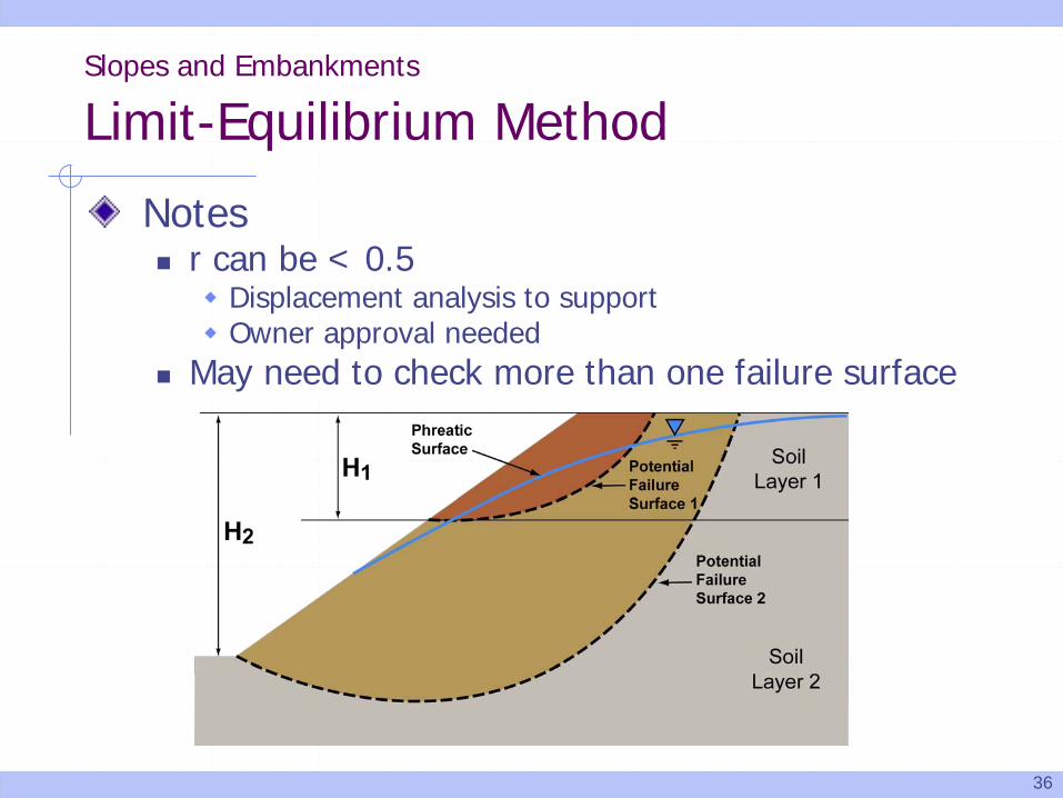
Slopes and Embankments
Limit-Equilibrium Method
Notes r can be < 0.5 Displacement analysis to support Owner approval needed
May need to check more than one failure surface

37
Pseudo-static analysis procedure – summary1. Find PGA and S1 from AASHTO hazard maps2. Find Site Class adjustment factors, FPGA & Fv
3. Find kmax = PGA x FPGA
4. Find β = S1FV/kmax = (SD1/kmax)5. Find scattering factor, α
If H < 20 ft, α = 1 If H ≥ 20 ft,
α = 1 + 0.01 H (0.5β – 1) Check H – iterate if necessary Limit H in α determination to 100 ft
Slopes and Embankments
Limit-Equilibrium Method
38
Pseudo-static analysis procedure – summary (cont.)5.Find kav = r α kmax
If ∆permissible = 1 to 2 in. or more, set r = 0.5 If ∆permissible < 1 to 2 in., set r = 1.0
6.Conduct pseudo-static stability analysis with kav If C/D (FS) ≥ 1.1, slope meets requirements If C/D (FS) ≤ 1.1
Implement mitigation Perform displacement analysis
Slopes and Embankments
Limit-Equilibrium Method
39
Slopes and Embankments
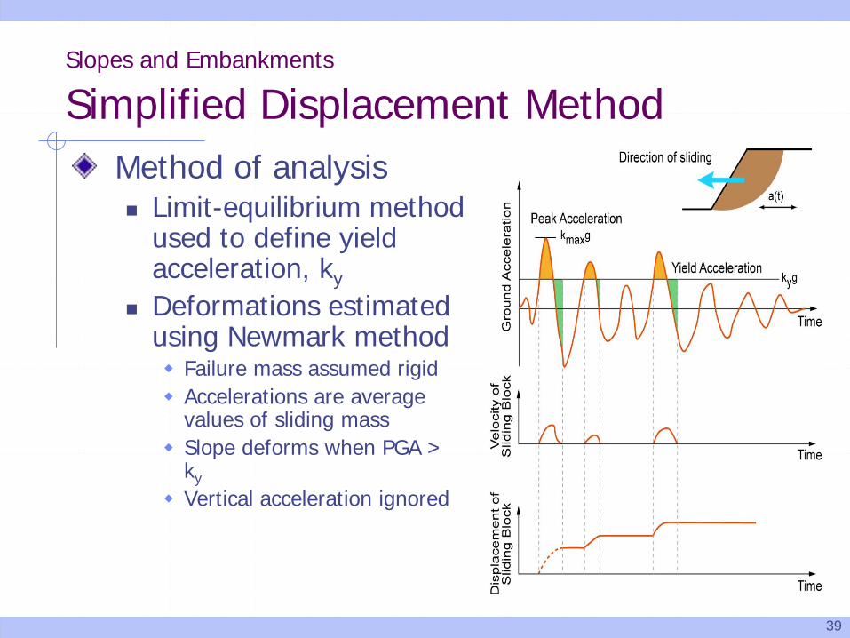
Simplified Displacement MethodMethod of analysis Limit-equilibrium method
used to define yield acceleration, ky
Deformations estimated using Newmark method Failure mass assumed rigid Accelerations are average
values of sliding mass Slope deforms when PGA >
ky
Vertical acceleration ignored
40
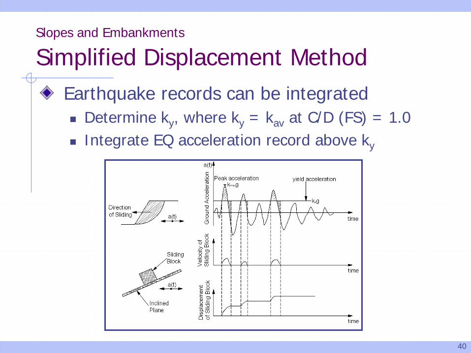
Earthquake records can be integrated Determine ky, where ky = kav at C/D (FS) = 1.0 Integrate EQ acceleration record above ky
Slopes and Embankments
Simplified Displacement Method
41
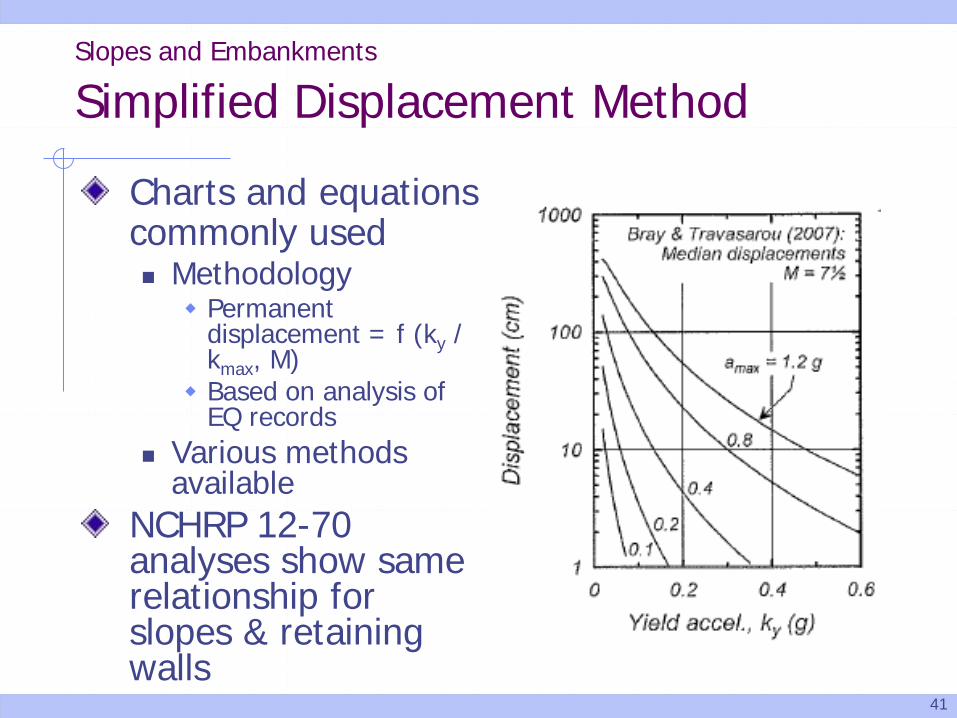
Charts and equations commonly used Methodology Permanent
displacement = f (ky / kmax, M)
Based on analysis of EQ records
Various methods available
NCHRP 12-70 analyses show same relationship for slopes & retaining walls
Slopes and Embankments
Simplified Displacement Method
42
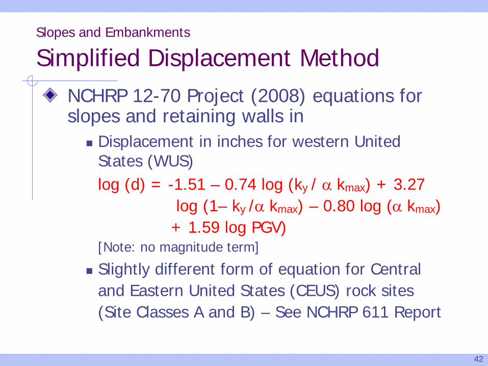
NCHRP 12-70 Project (2008) equations for slopes and retaining walls in
Displacement in inches for western United States (WUS)log (d) = -1.51 – 0.74 log (ky / α kmax) + 3.27
log (1– ky /α kmax) – 0.80 log (α kmax) + 1.59 log PGV)
[Note: no magnitude term]
Slightly different form of equation for Central and Eastern United States (CEUS) rock sites (Site Classes A and B) – See NCHRP 611 Report
Slopes and Embankments
Simplified Displacement Method
43
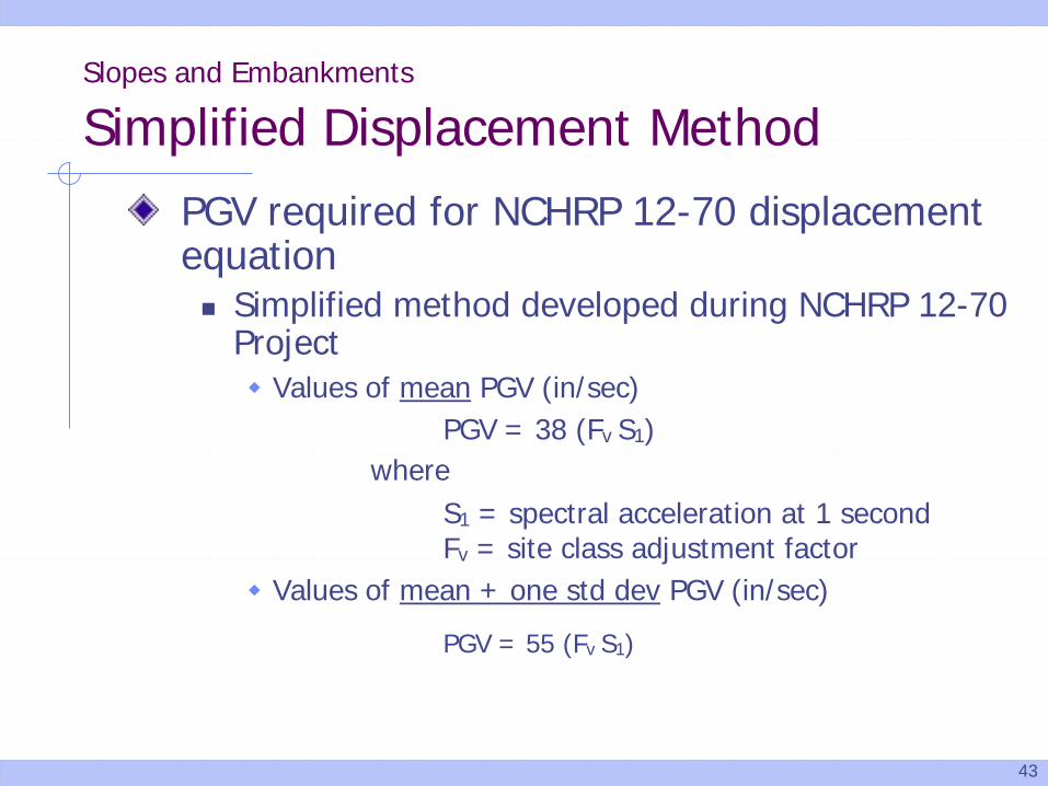
PGV required for NCHRP 12-70 displacement equation Simplified method developed during NCHRP 12-70
Project Values of mean PGV (in/sec)
PGV = 38 (Fv S1)where
S1 = spectral acceleration at 1 secondFv = site class adjustment factor
Values of mean + one std dev PGV (in/sec)
PGV = 55 (Fv S1)
Slopes and Embankments
Simplified Displacement Method
44
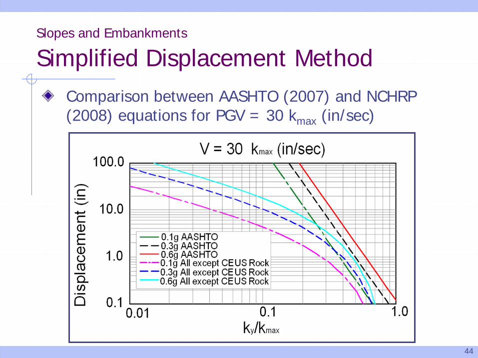
Comparison between AASHTO (2007) and NCHRP (2008) equations for PGV = 30 kmax (in/sec)
Slopes and Embankments
Simplified Displacement Method
45
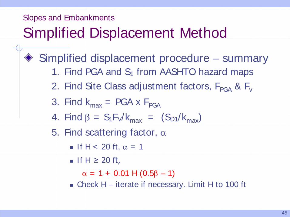
Simplified displacement procedure – summary 1. Find PGA and S1 from AASHTO hazard maps2. Find Site Class adjustment factors, FPGA & Fv
3. Find kmax = PGA x FPGA
4. Find β = S1FV/kmax = (SD1/kmax)
5. Find scattering factor, α If H < 20 ft, α = 1
If H ≥ 20 ft,
α = 1 + 0.01 H (0.5β – 1) Check H – iterate if necessary. Limit H to 100 ft
Slopes and Embankments
Simplified Displacement Method
46
Simplified displacement analysis procedure – summary (cont.)
6. Find ky from pseudo-static stability analysis
7. Estimate displacement potential using NCHRP 12-70 equation (or charts in NCHRP Report 611)
8. Evaluate acceptability of displacement based on performance criteria established by Owner
Slopes and Embankments
Simplified Displacement Method
47
Slopes and Embankments
Example
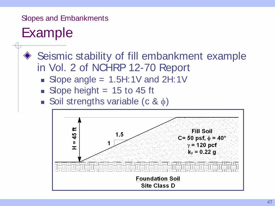
Seismic stability of fill embankment example in Vol. 2 of NCHRP 12-70 Report Slope angle = 1.5H:1V and 2H:1V Slope height = 15 to 45 ft Soil strengths variable (c & φ)
48
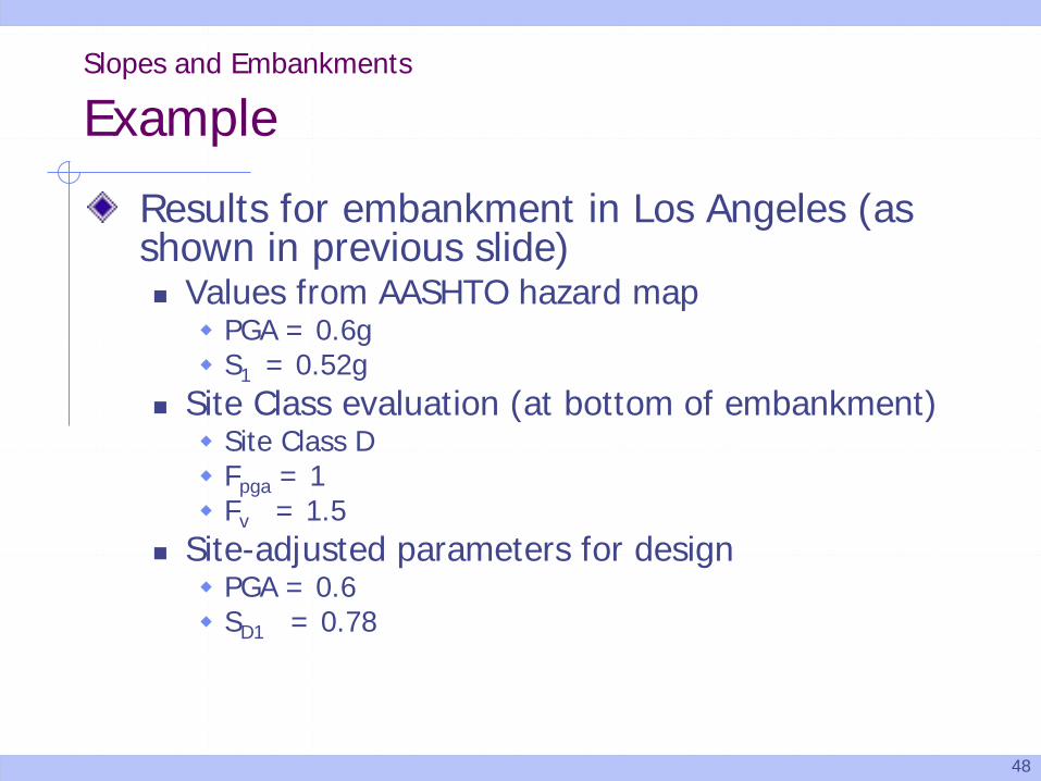
Results for embankment in Los Angeles (as shown in previous slide) Values from AASHTO hazard map PGA = 0.6g S1 = 0.52g
Site Class evaluation (at bottom of embankment) Site Class D Fpga = 1 Fv = 1.5
Site-adjusted parameters for design PGA = 0.6 SD1 = 0.78
Slopes and Embankments
Example
49
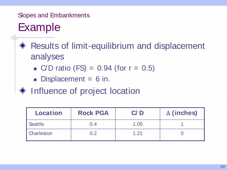
Results of limit-equilibrium and displacement analyses C/D ratio (FS) = 0.94 (for r = 0.5) Displacement = 6 in.
Influence of project location
Location Rock PGA C/D ∆ (inches)
Seattle 0.4 1.05 1
Charleston 0.2 1.21 0
Slopes and Embankments
Example
50
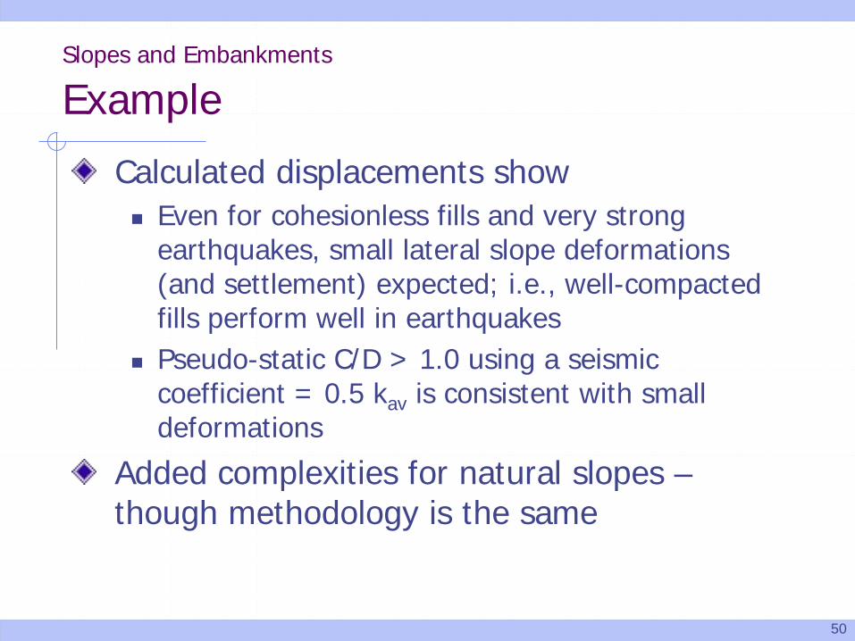
Calculated displacements show Even for cohesionless fills and very strong
earthquakes, small lateral slope deformations (and settlement) expected; i.e., well-compacted fills perform well in earthquakes
Pseudo-static C/D > 1.0 using a seismic coefficient = 0.5 kav is consistent with small deformations
Added complexities for natural slopes –though methodology is the same
Slopes and Embankments
Example
51
Slopes and Embankments
Special Consideration – Liquefaction
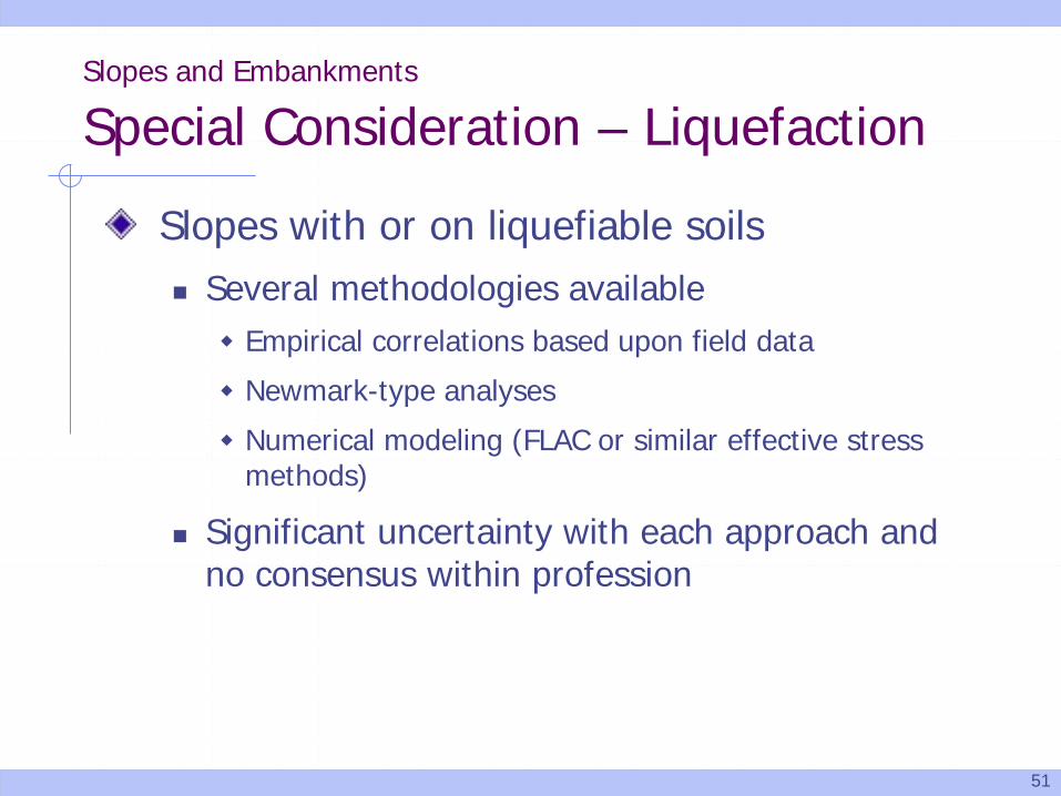
Slopes with or on liquefiable soils Several methodologies available Empirical correlations based upon field data
Newmark-type analyses
Numerical modeling (FLAC or similar effective stress methods)
Significant uncertainty with each approach and no consensus within profession
52
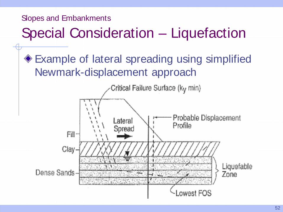
Example of lateral spreading using simplified Newmark-displacement approach
Slopes and Embankments
Special Consideration – Liquefaction
53
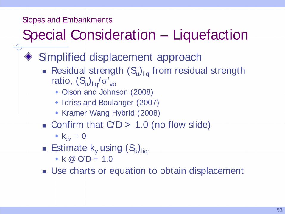
Simplified displacement approach Residual strength (Su)liq from residual strength
ratio, (Su)liq/σ’vo Olson and Johnson (2008) Idriss and Boulanger (2007) Kramer Wang Hybrid (2008)
Confirm that C/D > 1.0 (no flow slide) kav = 0
Estimate ky using (Su)liq. k @ C/D = 1.0
Use charts or equation to obtain displacement
Slopes and Embankments
Special Consideration – Liquefaction
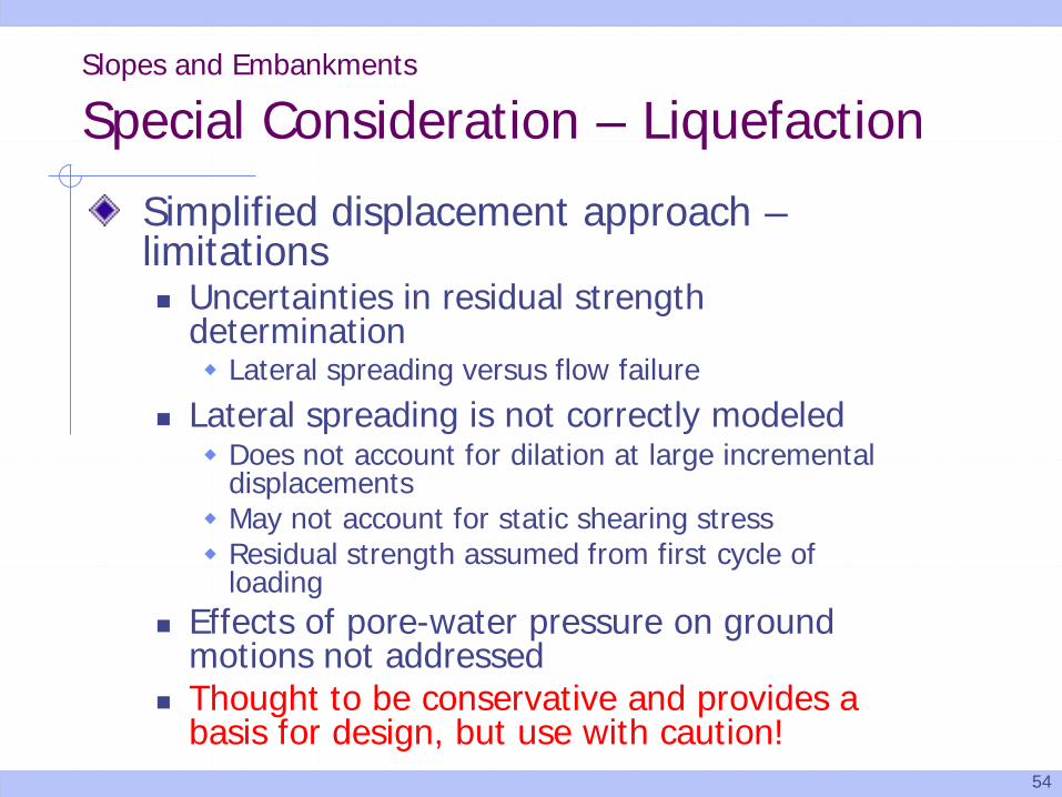
54
Simplified displacement approach –limitations Uncertainties in residual strength
determination Lateral spreading versus flow failure
Lateral spreading is not correctly modeled Does not account for dilation at large incremental
displacements May not account for static shearing stress Residual strength assumed from first cycle of
loading Effects of pore-water pressure on ground
motions not addressed Thought to be conservative and provides a
basis for design, but use with caution!
Slopes and Embankments
Special Consideration – Liquefaction
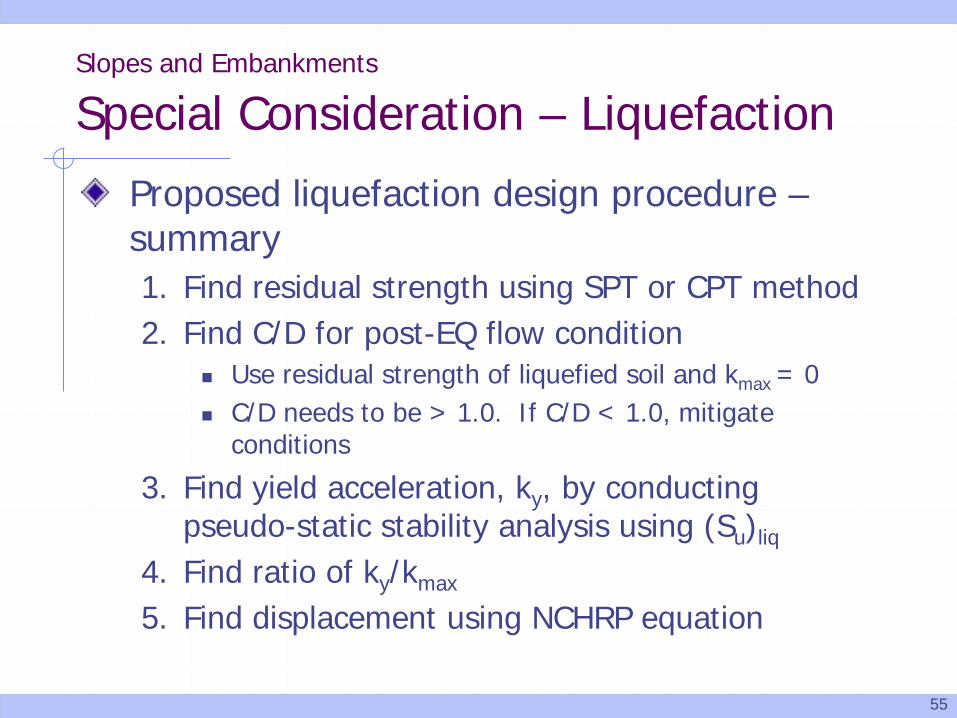
55
Proposed liquefaction design procedure –summary1. Find residual strength using SPT or CPT method2. Find C/D for post-EQ flow condition
Use residual strength of liquefied soil and kmax = 0 C/D needs to be > 1.0. If C/D < 1.0, mitigate
conditions
3. Find yield acceleration, ky, by conducting pseudo-static stability analysis using (Su)liq
4. Find ratio of ky/kmax
5. Find displacement using NCHRP equation
Slopes and Embankments
Special Consideration – Liquefaction
56
Slopes and Embankments
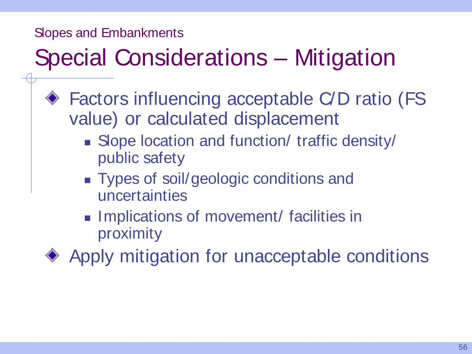
Special Considerations – Mitigation
Factors influencing acceptable C/D ratio (FS value) or calculated displacement Slope location and function/ traffic density/
public safety Types of soil/geologic conditions and
uncertainties Implications of movement/ facilities in
proximityApply mitigation for unacceptable conditions
57
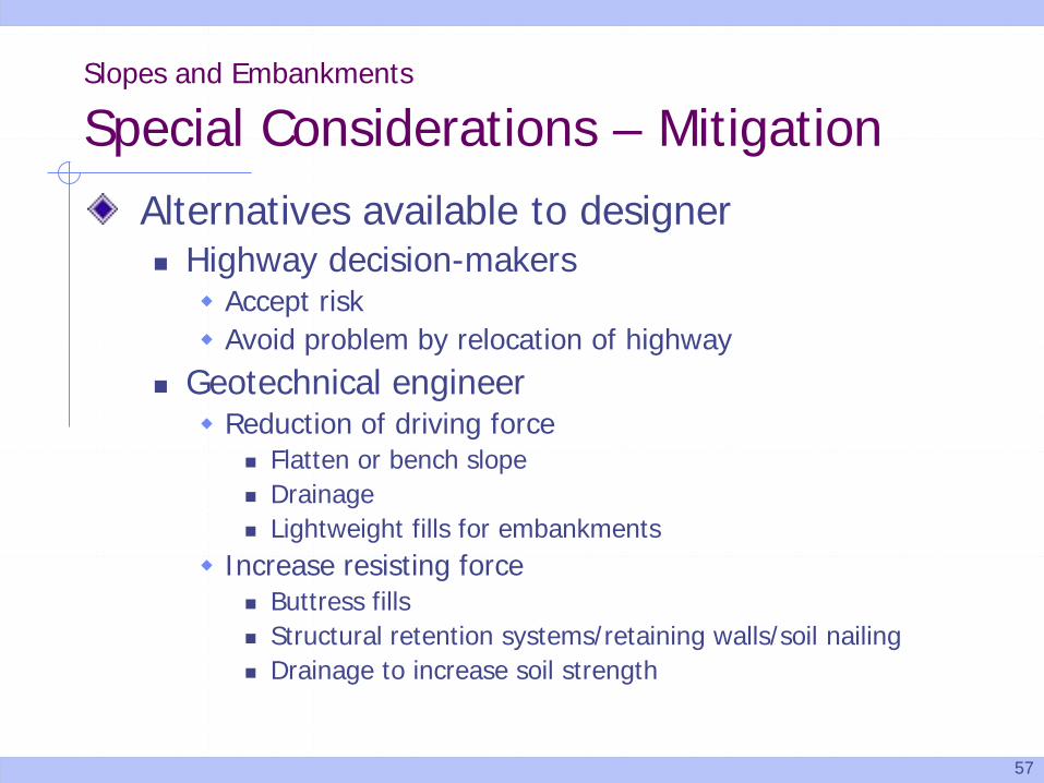
Alternatives available to designer Highway decision-makers Accept risk Avoid problem by relocation of highway
Geotechnical engineer Reduction of driving force
Flatten or bench slope Drainage Lightweight fills for embankments
Increase resisting force Buttress fills Structural retention systems/retaining walls/soil nailing Drainage to increase soil strength
Slopes and Embankments
Special Considerations – Mitigation
58
Slopes and Embankments
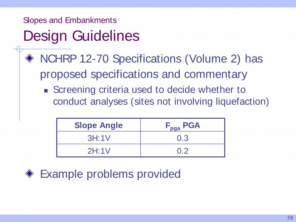
Design GuidelinesNCHRP 12-70 Specifications (Volume 2) has proposed specifications and commentary Screening criteria used to decide whether to
conduct analyses (sites not involving liquefaction)
Example problems provided
Slope Angle Fpga PGA3H:1V 0.3
2H:1V 0.2
59
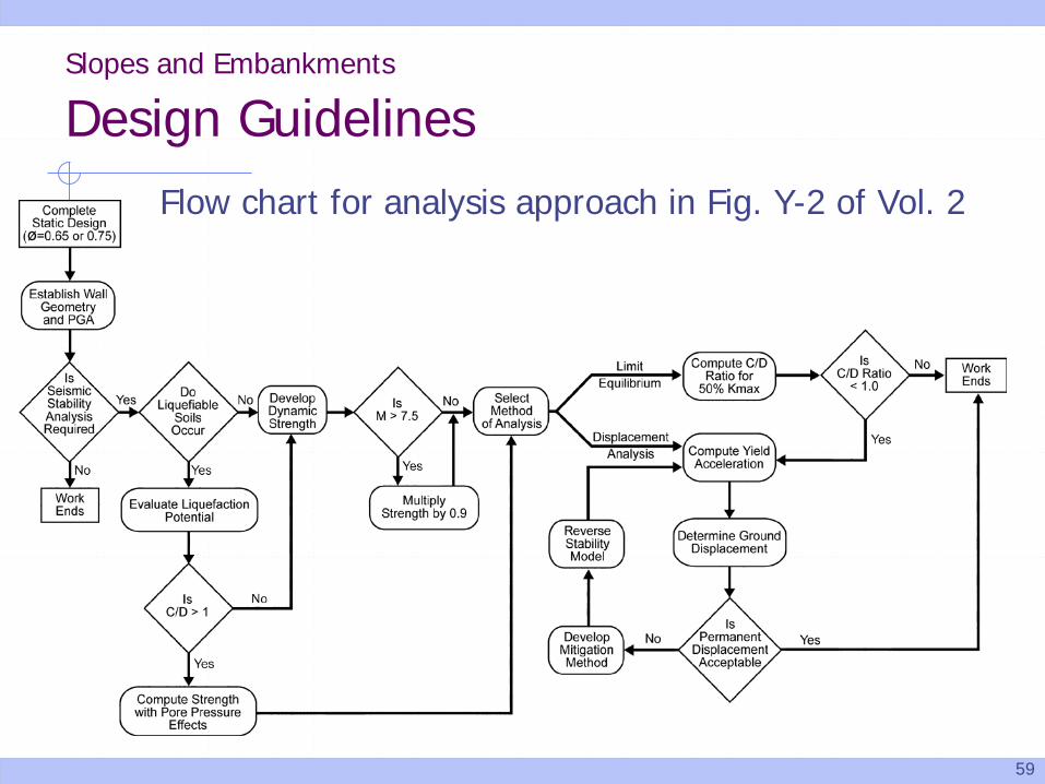
Flow chart for analysis approach in Fig. Y-2 of Vol. 2
Slopes and Embankments
Design Guidelines
60
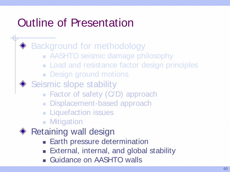
Outline of Presentation
Background for methodology AASHTO seismic damage philosophy Load and resistance factor design principles Design ground motions
Seismic slope stability Factor of safety (C/D) approach Displacement-based approach Liquefaction issues Mitigation
Retaining wall design Earth pressure determination External, internal, and global stability Guidance on AASHTO walls
61
Retaining Walls
Types of Walls
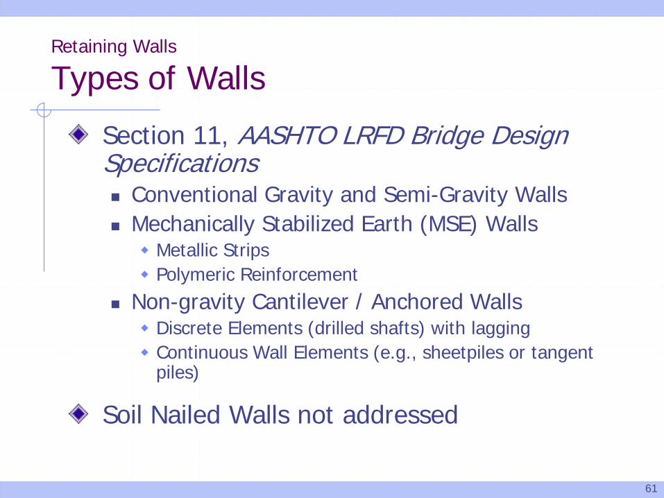
Section 11, AASHTO LRFD Bridge Design Specifications Conventional Gravity and Semi-Gravity Walls Mechanically Stabilized Earth (MSE) Walls Metallic Strips Polymeric Reinforcement
Non-gravity Cantilever / Anchored Walls Discrete Elements (drilled shafts) with lagging Continuous Wall Elements (e.g., sheetpiles or tangent
piles)
Soil Nailed Walls not addressed
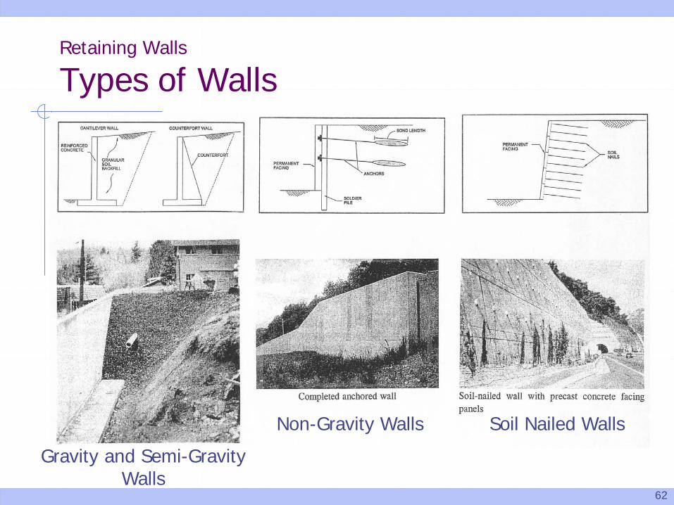
62
Retaining Walls
Types of Walls
Gravity and Semi-Gravity Walls
Non-Gravity Walls Soil Nailed Walls
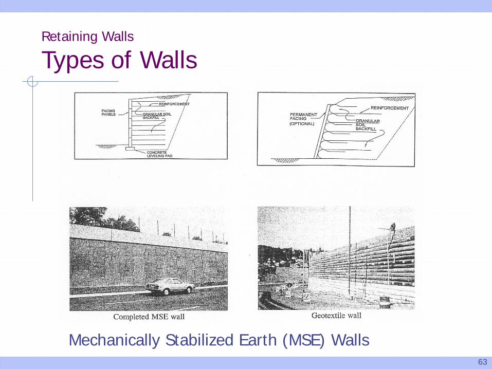
63
Mechanically Stabilized Earth (MSE) Walls
Retaining Walls
Types of Walls
64
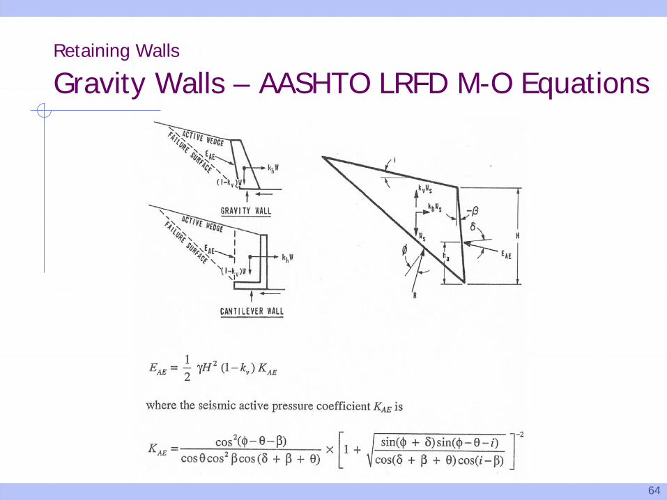
Retaining Walls
Gravity Walls – AASHTO LRFD M-O Equations
65
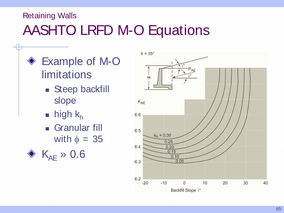
Retaining Walls
AASHTO LRFD M-O Equations
Example of M-O limitations Steep backfill
slope high kh
Granular fill with φ = 35
KAE » 0.6
66
Retaining Walls
AASHTO LRFD M-O Equations
Problems and knowledge gaps with M-O Equations Non-homogenous backfill and presence of
groundwater Sloping ground behind can give unrealistically
large seismic active pressure coefficients Rigid block sliding assumption – may not be
appropriate for wall heights > 30 ft Wall sliding assumption / displacement-based
design – not well understood & rotational displacement not considered
Existing charts do not consider seismic setting (e.g., WUS vs. CEUS)
67
Retaining Walls
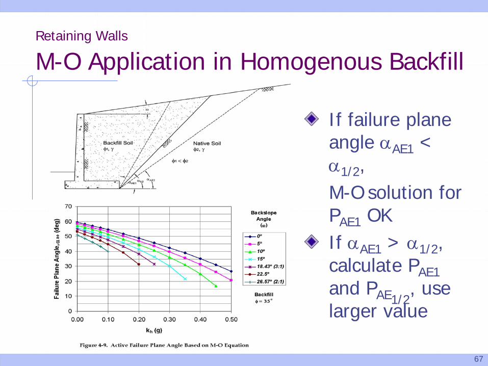
M-O Application in Homogenous Backfill
If failure plane angle αAE1 < α1/2,M-O solution for PAE1 OKIf αAE1 > α1/2, calculate PAE1and PAE1/2
, use larger value

68
Retaining Walls
Active Earth Pressures with CohesionM-O equations don’t account for cohesion Even small
cohesion (50 psf) give significant reductions in PAE
Charts have been developed based upon c/γH Apply with caution
in design practice due to uncertainties on c
69
Retaining Walls
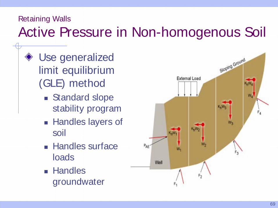
Active Pressure in Non-homogenous Soil
Use generalized limit equilibrium (GLE) method Standard slope
stability program Handles layers of
soil Handles surface
loads Handles
groundwater
70
Retaining Walls
Passive Earth Pressure
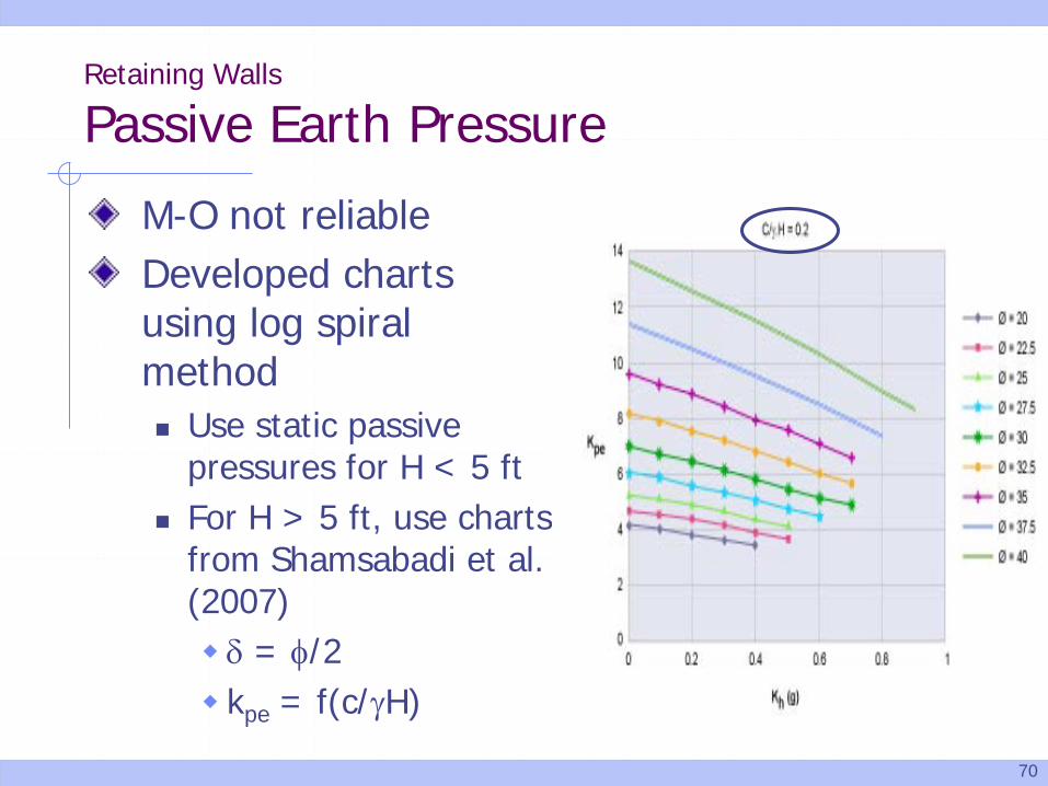
M-O not reliableDeveloped charts using log spiral method Use static passive
pressures for H < 5 ft For H > 5 ft, use charts
from Shamsabadi et al. (2007) δ = φ/2 kpe = f(c/γH)
71
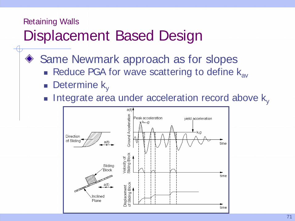
Retaining Walls
Displacement Based DesignSame Newmark approach as for slopes Reduce PGA for wave scattering to define kav
Determine ky
Integrate area under acceleration record above ky
72
Retaining Walls
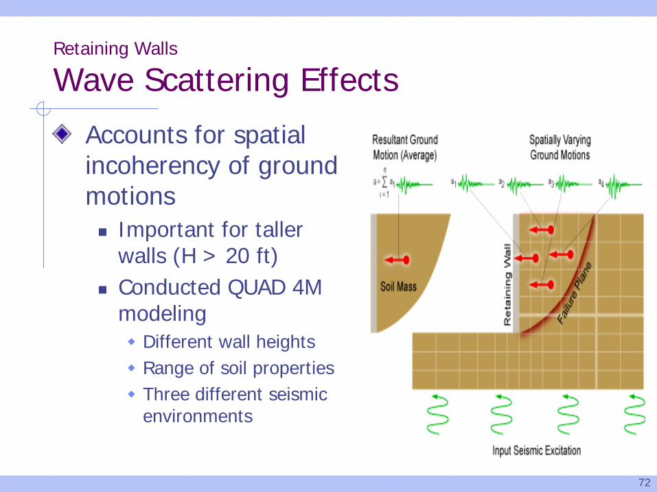
Wave Scattering Effects
Accounts for spatial incoherency of ground motions Important for taller
walls (H > 20 ft) Conducted QUAD 4M
modeling Different wall heights Range of soil properties Three different seismic
environments
73
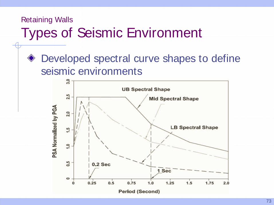
Retaining Walls
Types of Seismic Environment
Developed spectral curve shapes to define seismic environments

74
Retaining Walls
Height-Dependent Wave ScatteringDescribed by α factor: kav = α x PGA Use PGA corrected for
site class For Site Class C, D, and
Eα = 1 + 0.01H [0.5β - 1]
whereH = depth of failure surface β = FvS1/PGAα = 1.0 if H ≤ 20 ft
For Site Class A and B –increase computed α by 20%
75
Retaining Walls
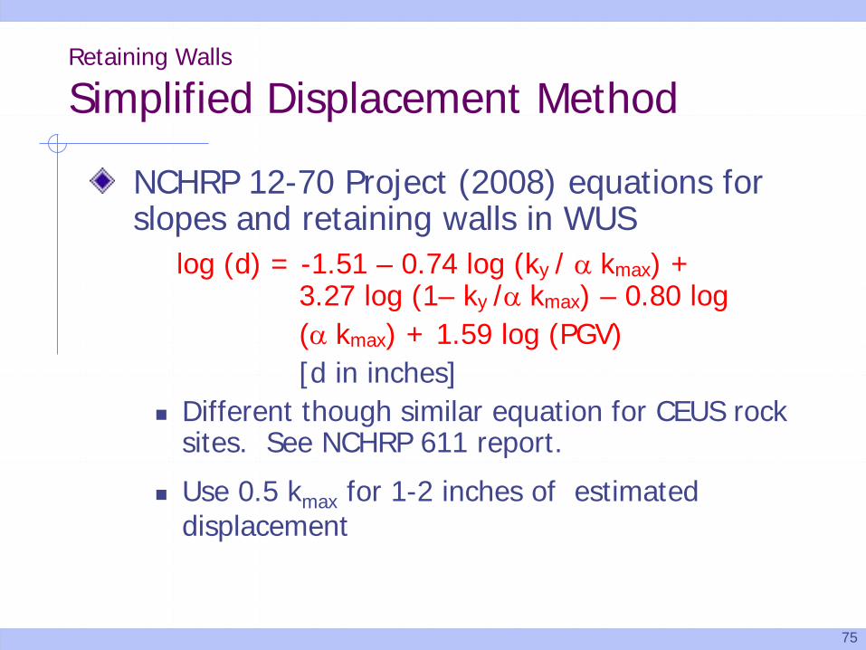
Simplified Displacement Method
NCHRP 12-70 Project (2008) equations for slopes and retaining walls in WUS
log (d) = -1.51 – 0.74 log (ky / α kmax) + 3.27 log (1– ky /α kmax) – 0.80 log (α kmax) + 1.59 log (PGV)[d in inches]
Different though similar equation for CEUS rock sites. See NCHRP 611 report.
Use 0.5 kmax for 1-2 inches of estimated displacement
76
Retaining Walls
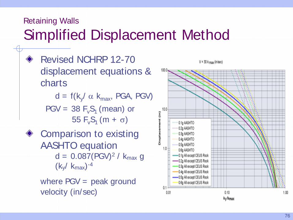
Simplified Displacement Method
Revised NCHRP 12-70 displacement equations & charts
d = f(ky/ α kmax, PGA, PGV)
PGV = 38 FvS1 (mean) or 55 FvS1 (m + σ)
Comparison to existing AASHTO equation
d = 0.087(PGV)2 / kmax g (ky/ kmax)-4
where PGV = peak ground velocity (in/sec)
77
Retaining Walls
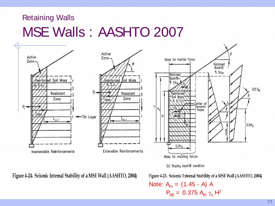
MSE Walls : AASHTO 2007
Note: Am = (1.45 - A) APAE = 0.375 Am γs H2
78
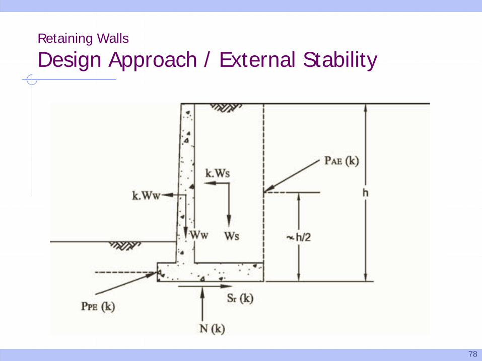
Retaining Walls
Design Approach / External Stability
79
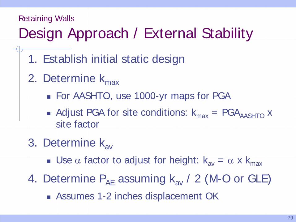
Retaining Walls
Design Approach / External Stability
1. Establish initial static design
2. Determine kmax
For AASHTO, use 1000-yr maps for PGA
Adjust PGA for site conditions: kmax = PGAAASHTO x site factor
3. Determine kav
Use α factor to adjust for height: kav = α x kmax
4. Determine PAE assuming kav / 2 (M-O or GLE) Assumes 1-2 inches displacement OK
80
Retaining Walls
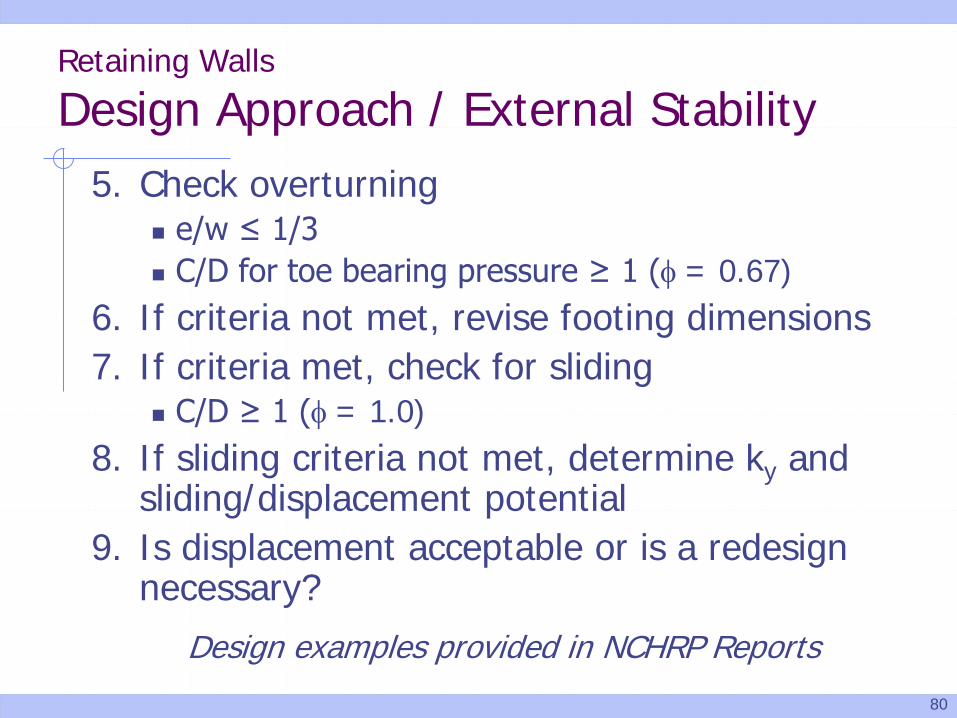
Design Approach / External Stability5. Check overturning
e/w ≤ 1/3 C/D for toe bearing pressure ≥ 1 (φ = 0.67)
6. If criteria not met, revise footing dimensions7. If criteria met, check for sliding
C/D ≥ 1 (φ = 1.0)8. If sliding criteria not met, determine ky and
sliding/displacement potential9. Is displacement acceptable or is a redesign
necessary?
Design examples provided in NCHRP Reports
81
Retaining Walls
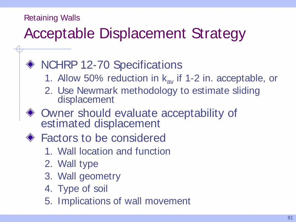
Acceptable Displacement Strategy
NCHRP 12-70 Specifications1. Allow 50% reduction in kav if 1-2 in. acceptable, or2. Use Newmark methodology to estimate sliding
displacementOwner should evaluate acceptability of estimated displacementFactors to be considered1. Wall location and function2. Wall type3. Wall geometry4. Type of soil5. Implications of wall movement
82
Retaining Walls
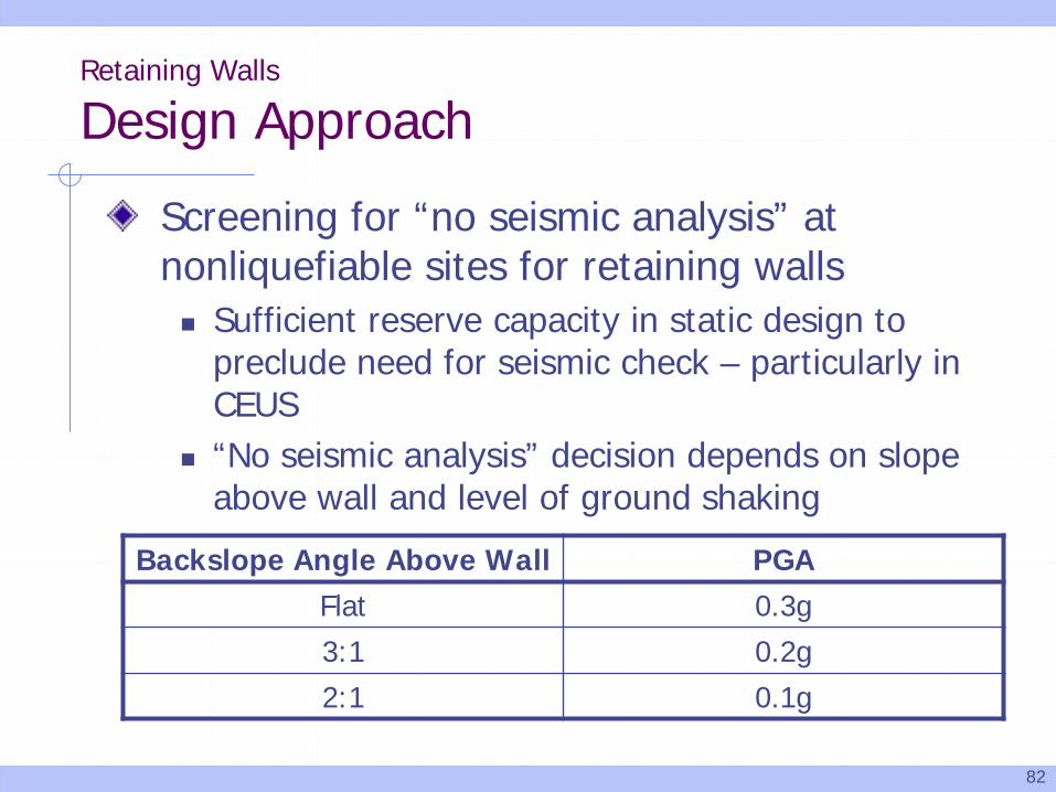
Design Approach
Screening for “no seismic analysis” at nonliquefiable sites for retaining walls Sufficient reserve capacity in static design to
preclude need for seismic check – particularly in CEUS
“No seismic analysis” decision depends on slope above wall and level of ground shaking
Backslope Angle Above Wall PGAFlat 0.3g
3:1 0.2g
2:1 0.1g
83
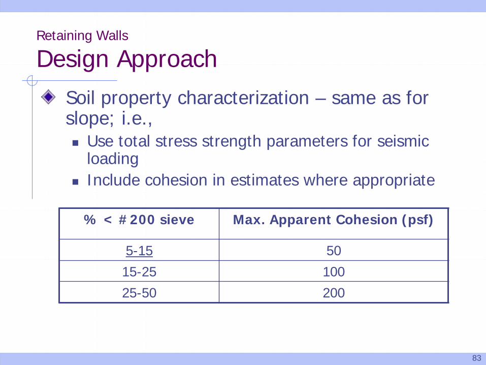
Retaining Walls
Design ApproachSoil property characterization – same as for slope; i.e., Use total stress strength parameters for seismic
loading Include cohesion in estimates where appropriate
% < #200 sieve Max. Apparent Cohesion (psf)
5-15 50
15-25 100
25-50 200
84
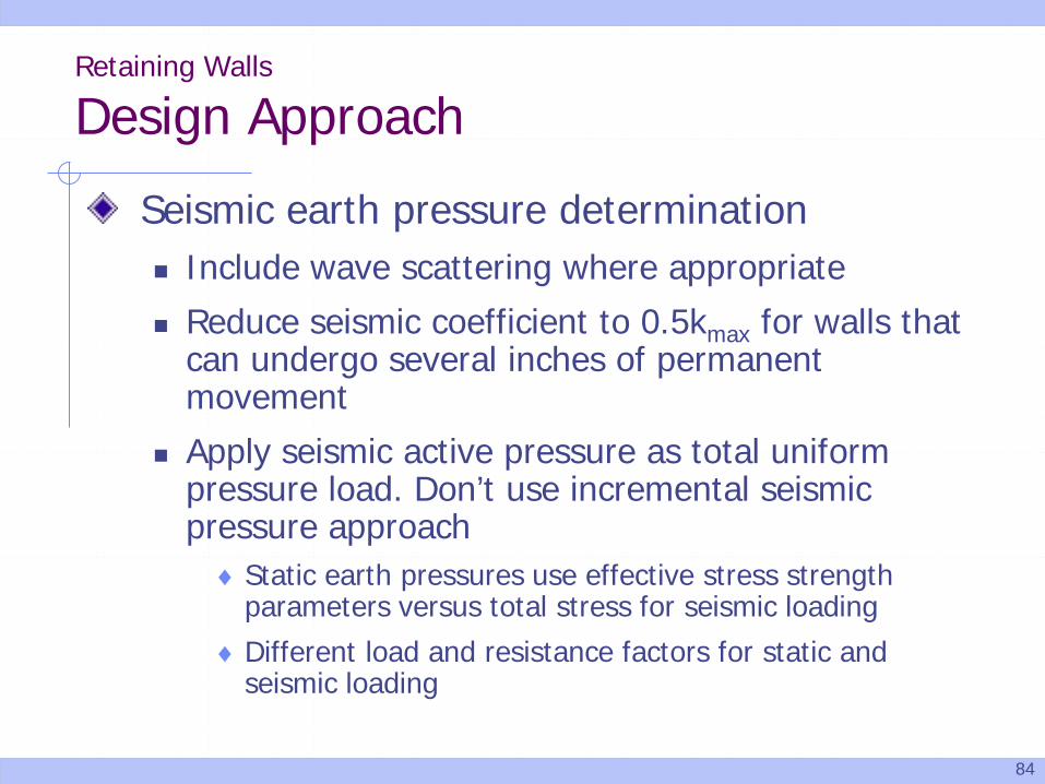
Retaining Walls
Design Approach
Seismic earth pressure determination Include wave scattering where appropriate
Reduce seismic coefficient to 0.5kmax for walls that can undergo several inches of permanent movement
Apply seismic active pressure as total uniform pressure load. Don’t use incremental seismic pressure approach
♦ Static earth pressures use effective stress strength parameters versus total stress for seismic loading
♦ Different load and resistance factors for static and seismic loading
85
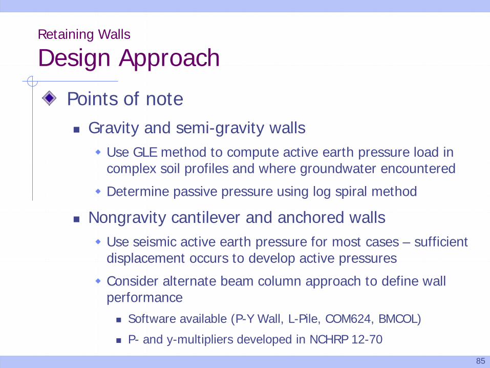
Retaining Walls
Design Approach
Points of note Gravity and semi-gravity walls Use GLE method to compute active earth pressure load in
complex soil profiles and where groundwater encountered
Determine passive pressure using log spiral method
Nongravity cantilever and anchored walls Use seismic active earth pressure for most cases – sufficient
displacement occurs to develop active pressures
Consider alternate beam column approach to define wall performance Software available (P-Y Wall, L-Pile, COM624, BMCOL)
P- and y-multipliers developed in NCHRP 12-70
86
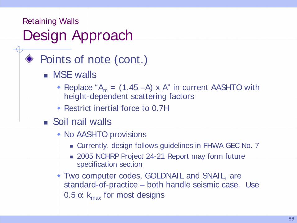
Retaining Walls
Design ApproachPoints of note (cont.) MSE walls Replace “Am = (1.45 –A) x A” in current AASHTO with
height-dependent scattering factors Restrict inertial force to 0.7H
Soil nail walls No AASHTO provisions
Currently, design follows guidelines in FHWA GEC No. 7 2005 NCHRP Project 24-21 Report may form future
specification section
Two computer codes, GOLDNAIL and SNAIL, are standard-of-practice – both handle seismic case. Use 0.5 α kmax for most designs
87
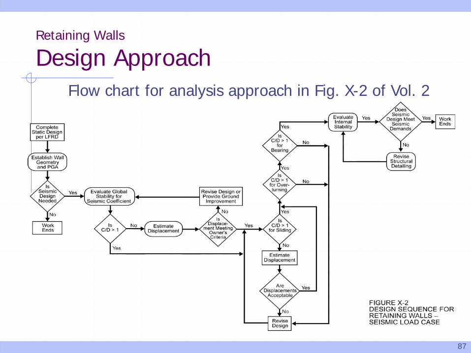
Retaining Walls
Design ApproachFlow chart for analysis approach in Fig. X-2 of Vol. 2
88
Slopes, Embankments & Retaining Walls
Concluding CommentsNCHRP Report 611 provides framework for update to AASHTO LRFD Bridge Design Specifications More design checks needed
Are screening levels appropriate? Are proposed methodologies consistent with other numerical
results, model testing, and field experiments?
Further studies and development required in some areas Does shear banding occur in cohesionless soils? How should inertial force in MSE wall be defined? Will soil-structure interaction affect ground motions adjacent to
nongravity cantilever and anchored walls? What is total seismic pressure distribution behind gravity,
cantilever, and anchored walls?