Seismic Anisotropy and shear-wave splitting

Steve Gao, Missouri S&T

http://www.mst.edu/~sgao

1

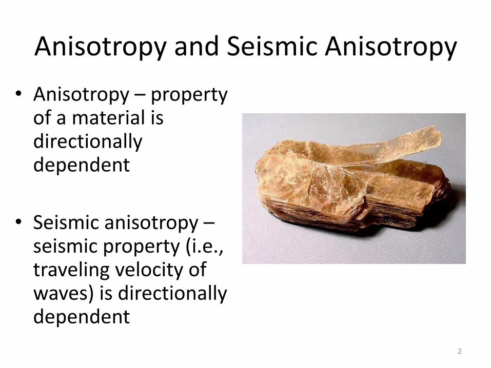
Anisotropy and Seismic Anisotropy

• Anisotropy – property of a material is directionally dependent

• Seismic anisotropy – seismic property (i.e., traveling velocity of waves) is directionally dependent

2

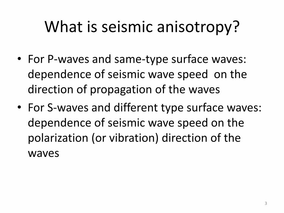
What is seismic anisotropy?

• For P-waves and same-type surface waves: dependence of seismic wave speed on the direction of propagation of the waves

• For S-waves and different type surface waves: dependence of seismic wave speed on the polarization (or vibration) direction of the waves

3

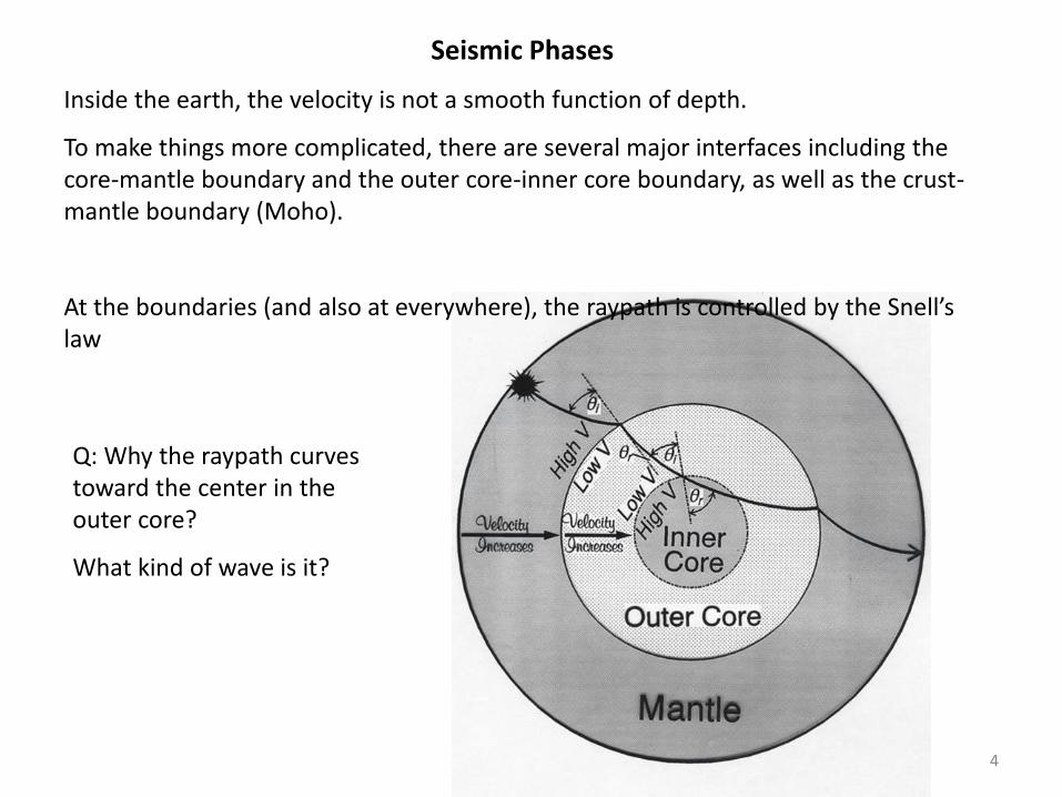
Seismic Phases

Inside the earth, the velocity is not a smooth function of depth.

To make things more complicated, there are several major interfaces including the core-mantle boundary and the outer core-inner core boundary, as well as the crust-mantle boundary (Moho).

At the boundaries (and also at everywhere), the raypath is controlled by the Snell’s law

Q: Why the raypath curves toward the center in the outer core?

What kind of wave is it?

4

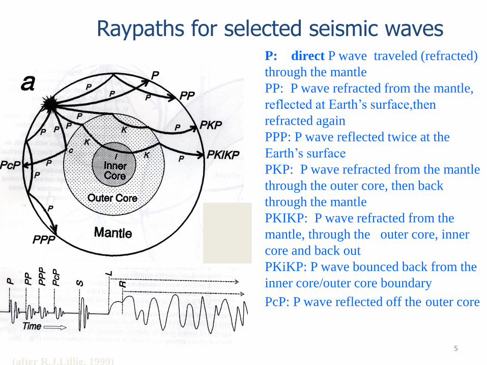
Raypaths for selected seismic waves

(after R.J.Lillie, 1999)

P: direct P wave traveled (refracted)

through the mantle

PP: P wave refracted from the mantle,

reflected at Earth’s surface,then

refracted again

PPP: P wave reflected twice at the

Earth’s surface

PKP: P wave refracted from the mantle

through the outer core, then back

through the mantle

PKIKP: P wave refracted from the

mantle, through the outer core, inner

core and back out

PKiKP: P wave bounced back from the

inner core/outer core boundary

PcP: P wave reflected off the outer core

5

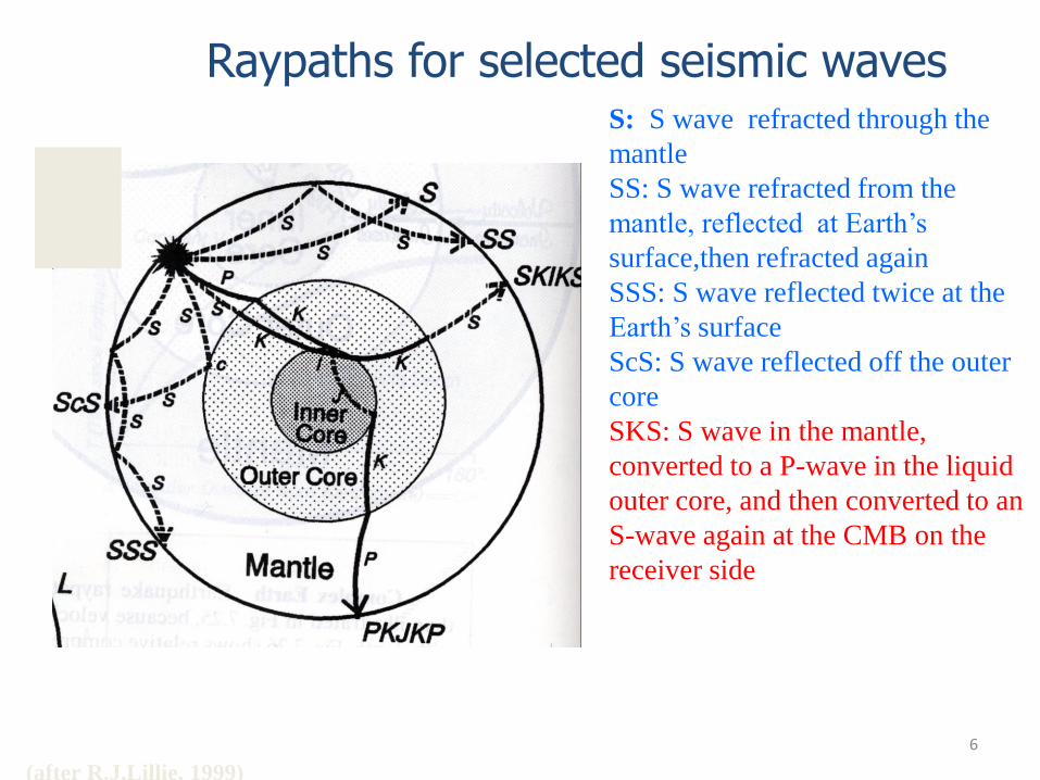
Raypaths for selected seismic waves S: S wave refracted through the

mantle

SS: S wave refracted from the

mantle, reflected at Earth’s

surface,then refracted again

SSS: S wave reflected twice at the

Earth’s surface

ScS: S wave reflected off the outer

core

SKS: S wave in the mantle,

converted to a P-wave in the liquid

outer core, and then converted to an

S-wave again at the CMB on the

receiver side

(after R.J.Lillie, 1999)

6

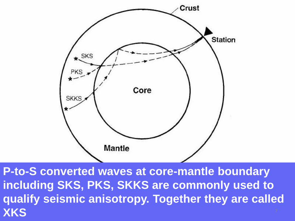
P-to-S converted waves at core-mantle boundary

including SKS, PKS, SKKS are commonly used to

qualify seismic anisotropy. Together they are called

XKS 7

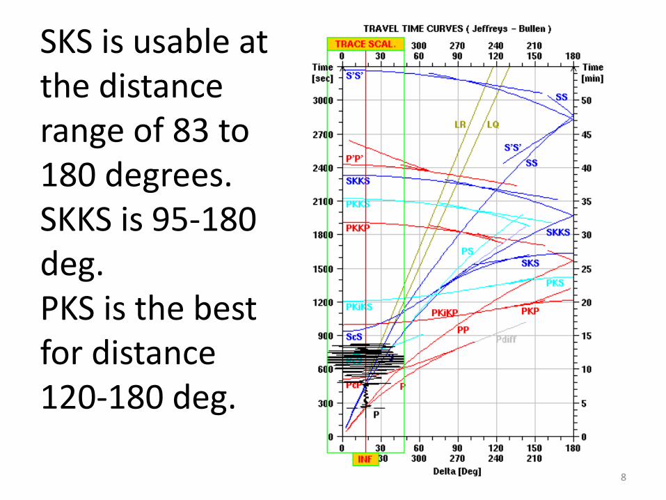
SKS is usable at the distance range of 83 to 180 degrees. SKKS is 95-180 deg. PKS is the best for distance 120-180 deg.

8

What is shear-wave splitting?

• When a shear-wave propagates through a layer of anisotropy, it splits into two waves with orthogonal direction of vibration (polarization).

9

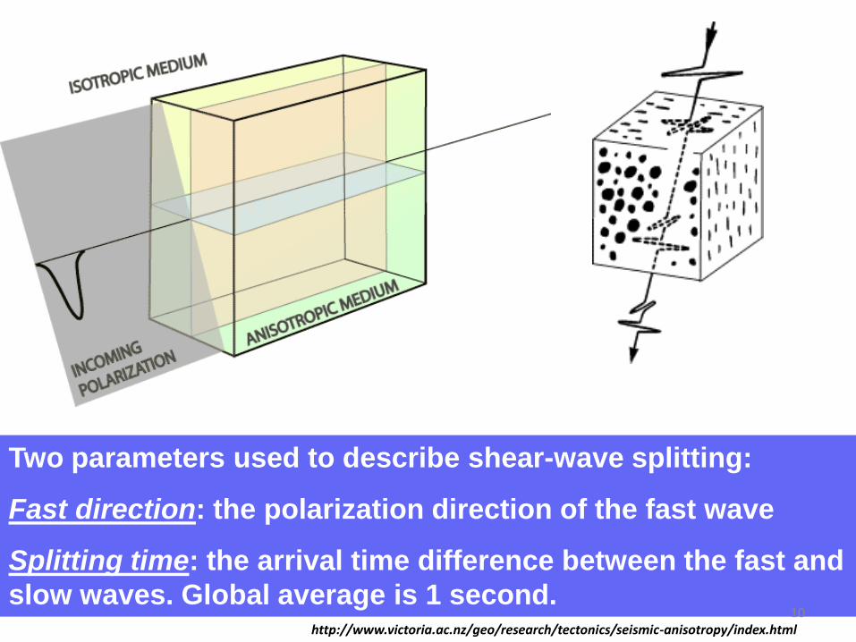
http://www.victoria.ac.nz/geo/research/tectonics/seismic-anisotropy/index.html

Two parameters used to describe shear-wave splitting:

Fast direction: the polarization direction of the fast wave

Splitting time: the arrival time difference between the fast and

slow waves. Global average is 1 second. 10

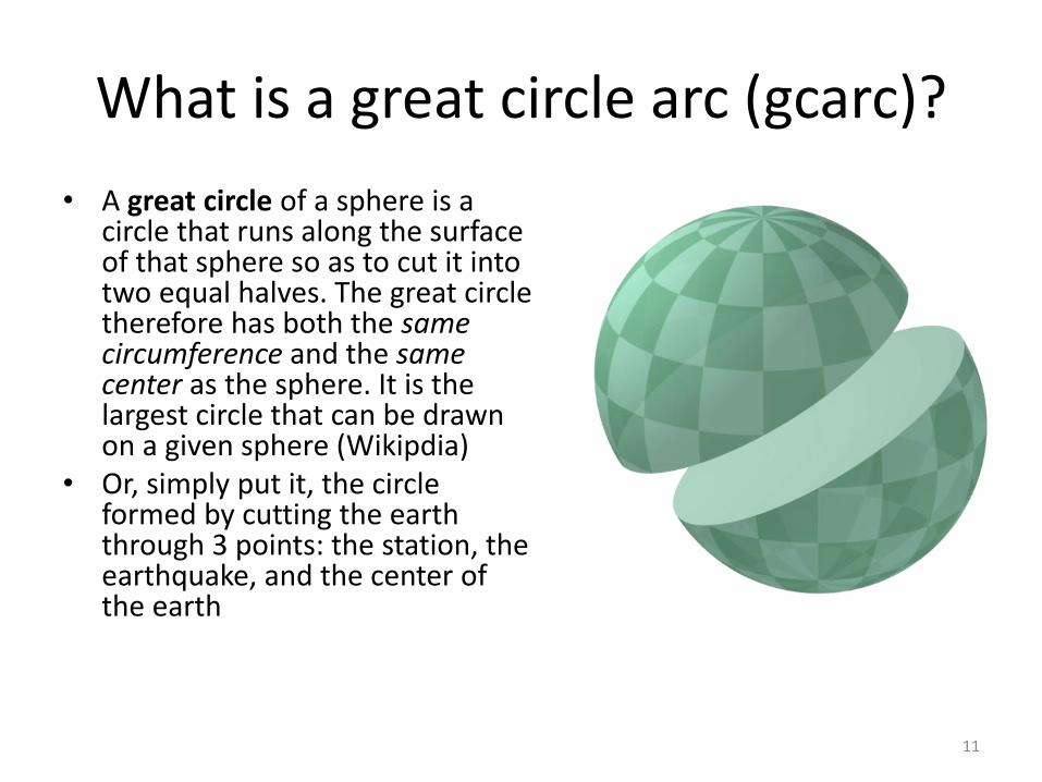
What is a great circle arc (gcarc)?

• A great circle of a sphere is a circle that runs along the surface of that sphere so as to cut it into two equal halves. The great circle therefore has both the same circumference and the same center as the sphere. It is the largest circle that can be drawn on a given sphere (Wikipdia)

• Or, simply put it, the circle formed by cutting the earth through 3 points: the station, the earthquake, and the center of the earth

11

Back-azimuth of an earthquake relative to the station

• The azimuth of the gcarc measured clockwise from the North.

• For instance, an earthquake coming from the east has a BAZ of 90 deg., and one from the west has a BAZ of 270 deg.

12

Radial and transverse components of a shear-wave

• The shear-wave that vibrates along the BAZ direction when projected to the surface of the earth is the radial component. If the ray-path only travels through isotropic media, all the XKS energy should be on the radial component

• The shear-wave that vibrates along the direction that is orthogonal to the BAZ direction when projected to the surface is the transverse component

13

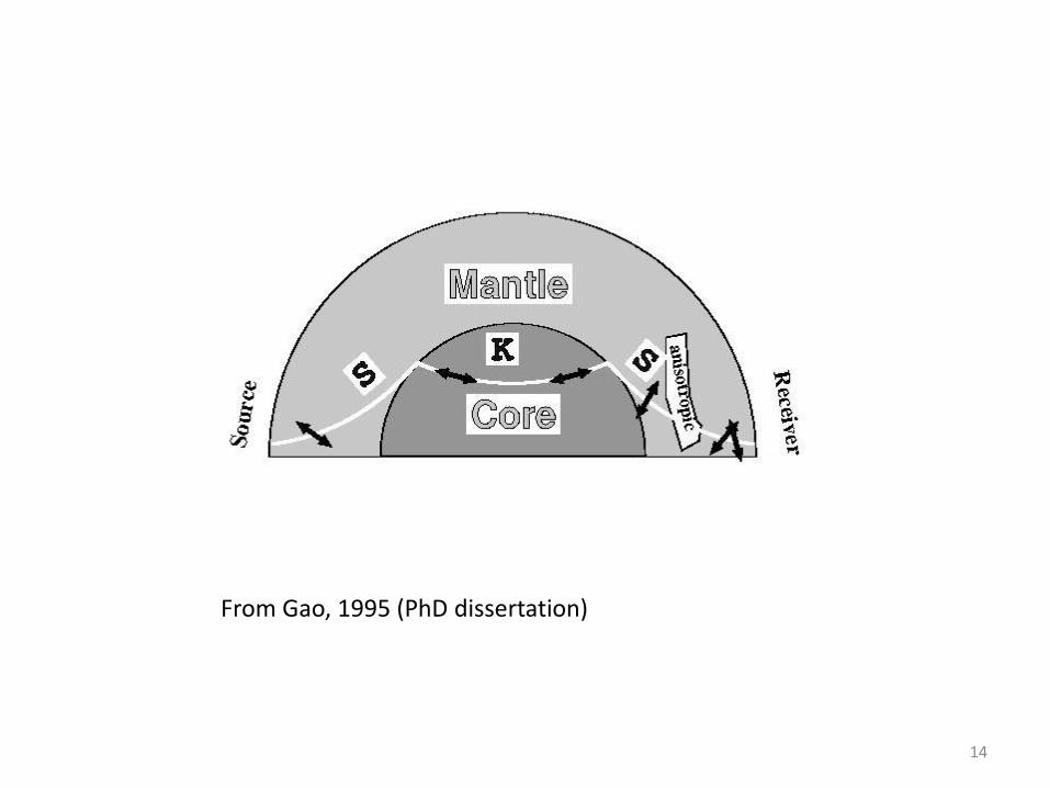
From Gao, 1995 (PhD dissertation)

14

Ray parameter

• A number with a unit of second/degree. It is basically a measure of the angle of incidence (measured from the vertical) of a seismic wave.

• It can be understood as: for two stations that are 1 degree apart (111.19 km) on the surface, the difference in arrival time for a seismic ray with a ray parameter of RP between the two stations is RP seconds.

• The RP for SKS is from 0 to about 6.5 s/deg., this means that the angle of incidence is from 0 to about 25 degrees from the vertical. SKKS and PKS have similar RP.

15

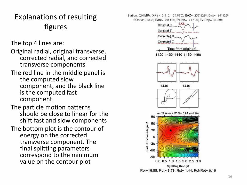
Explanations of resulting figures

The top 4 lines are: Original radial, original transverse,

corrected radial, and corrected transverse components

The red line in the middle panel is the computed slow component, and the black line is the computed fast component

The particle motion patterns should be close to linear for the shift fast and slow components

The bottom plot is the contour of energy on the corrected transverse component. The final splitting parameters correspond to the minimum value on the contour plot

16

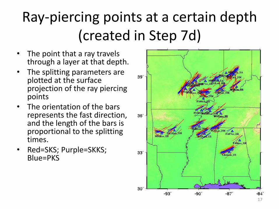
Ray-piercing points at a certain depth (created in Step 7d)

• The point that a ray travels through a layer at that depth.

• The splitting parameters are plotted at the surface projection of the ray piercing points

• The orientation of the bars represents the fast direction, and the length of the bars is proportional to the splitting times.

• Red=SKS; Purple=SKKS; Blue=PKS

17

Modulo?

• Modulo-90 degree is computed as such: • If the BAZ is less than 90 deg., the Modulo-90 is the

same as the BAZ • If the BAZ is between 90 and 180, the Modulo-90 is

BAZ minus 90 • If the BAZ is between 180 and 270, the Modulo-90 is

BAZ minus 180. • If the BAZ is between 270 and 360, the Modulo-90 is

BAZ minus 270. • Variation of splitting parameters with Modulo-90 is

used to identify 90-degree periodicity

18

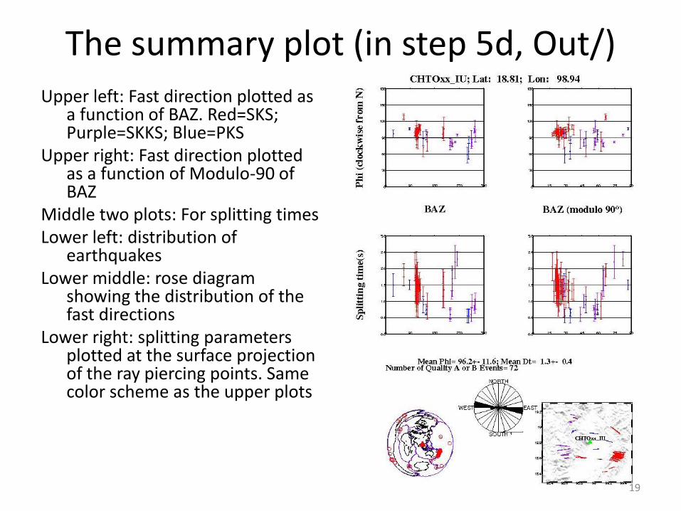
The summary plot (in step 5d, Out/) Upper left: Fast direction plotted as

a function of BAZ. Red=SKS; Purple=SKKS; Blue=PKS

Upper right: Fast direction plotted as a function of Modulo-90 of BAZ

Middle two plots: For splitting times Lower left: distribution of

earthquakes Lower middle: rose diagram

showing the distribution of the fast directions

Lower right: splitting parameters plotted at the surface projection of the ray piercing points. Same color scheme as the upper plots

19

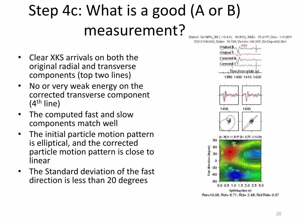
Step 4c: What is a good (A or B) measurement?

• Clear XKS arrivals on both the original radial and transverse components (top two lines)

• No or very weak energy on the corrected transverse component (4th line)

• The computed fast and slow components match well

• The initial particle motion pattern is elliptical, and the corrected particle motion pattern is close to linear

• The Standard deviation of the fast direction is less than 20 degrees

20

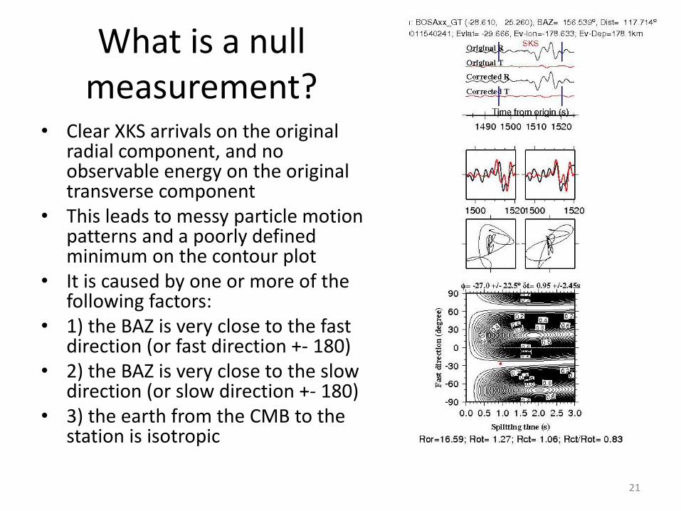
What is a null measurement?

• Clear XKS arrivals on the original radial component, and no observable energy on the original transverse component

• This leads to messy particle motion patterns and a poorly defined minimum on the contour plot

• It is caused by one or more of the following factors:

• 1) the BAZ is very close to the fast direction (or fast direction +- 180)

• 2) the BAZ is very close to the slow direction (or slow direction +- 180)

• 3) the earth from the CMB to the station is isotropic

21

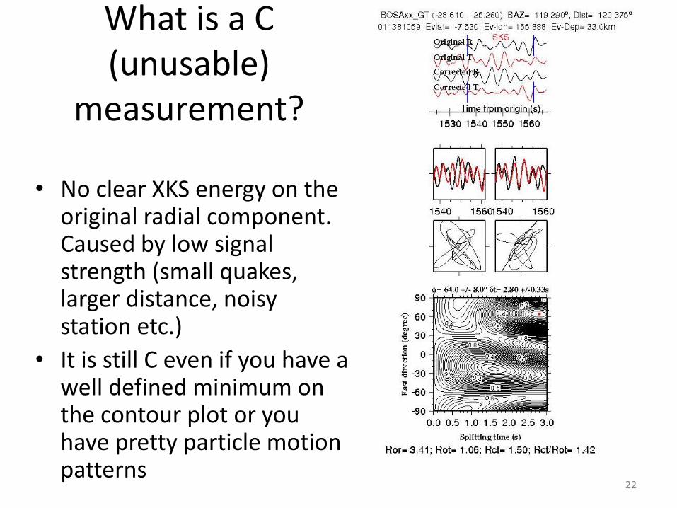
What is a C (unusable)

measurement?

• No clear XKS energy on the original radial component. Caused by low signal strength (small quakes, larger distance, noisy station etc.)

• It is still C even if you have a well defined minimum on the contour plot or you have pretty particle motion patterns

22

Reading Assignment

• Paper A15 under http://web.mst.edu/~sgao/publications/index1.html

23

What is ‘simple anisotropy’?

• Simple anisotropy (that can be detected by shear-wave splitting) is created by a single layer of rocks. The fast and slow axes are both located on the horizontal plane

• The splitting parameters (fast directions and splitting times) do not change as functions of the arriving azimuth (back azimuth) of the events. Therefore, the parameters are normally averaged over all the events from a station.

• The vast majority (~95%) of all the previous published papers assume simple anisotropy

24

What is complex anisotropy?

• Any other situation that is not simple anisotropy is complex anisotropy

• Most common situations of complex anisotropy 1). Double layer: two layers with horizontal axes and

different fast directions. This is the most common case of complex anisotropy and is the subject of today’s lecture

2). Three or more horizontal layers 3). Single layer with tilting axes – the splitting parameters

vary as a function of the back azimuth with a period of 180 degrees.

4). Any combinations of the above 3 cases.

25

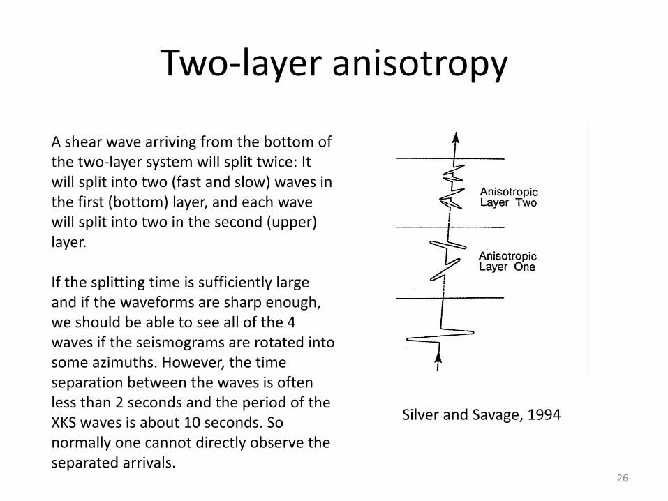
Two-layer anisotropy

Silver and Savage, 1994

A shear wave arriving from the bottom of the two-layer system will split twice: It will split into two (fast and slow) waves in the first (bottom) layer, and each wave will split into two in the second (upper) layer. If the splitting time is sufficiently large and if the waveforms are sharp enough, we should be able to see all of the 4 waves if the seismograms are rotated into some azimuths. However, the time separation between the waves is often less than 2 seconds and the period of the XKS waves is about 10 seconds. So normally one cannot directly observe the separated arrivals.

26

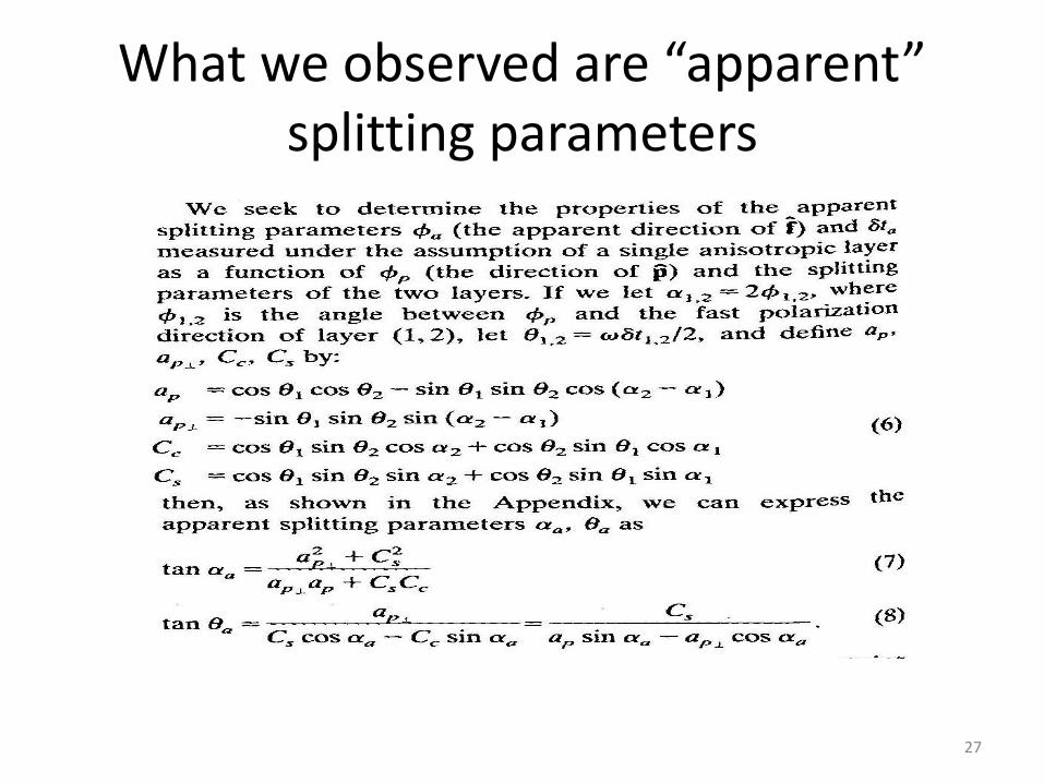
What we observed are “apparent” splitting parameters

27

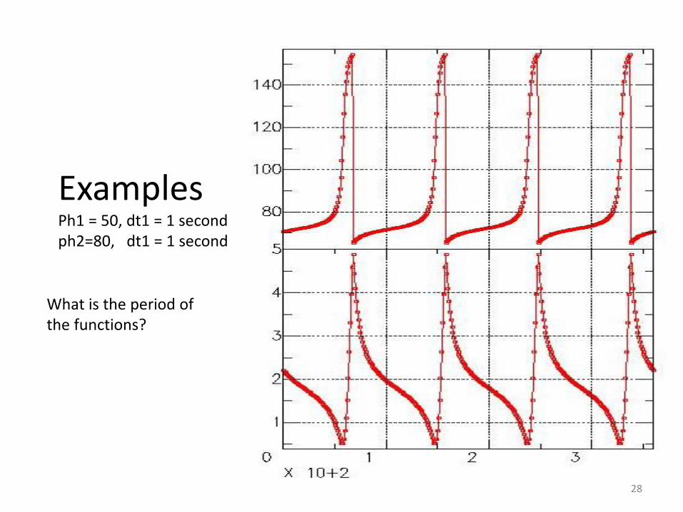
Examples Ph1 = 50, dt1 = 1 second ph2=80, dt1 = 1 second

What is the period of the functions?

28

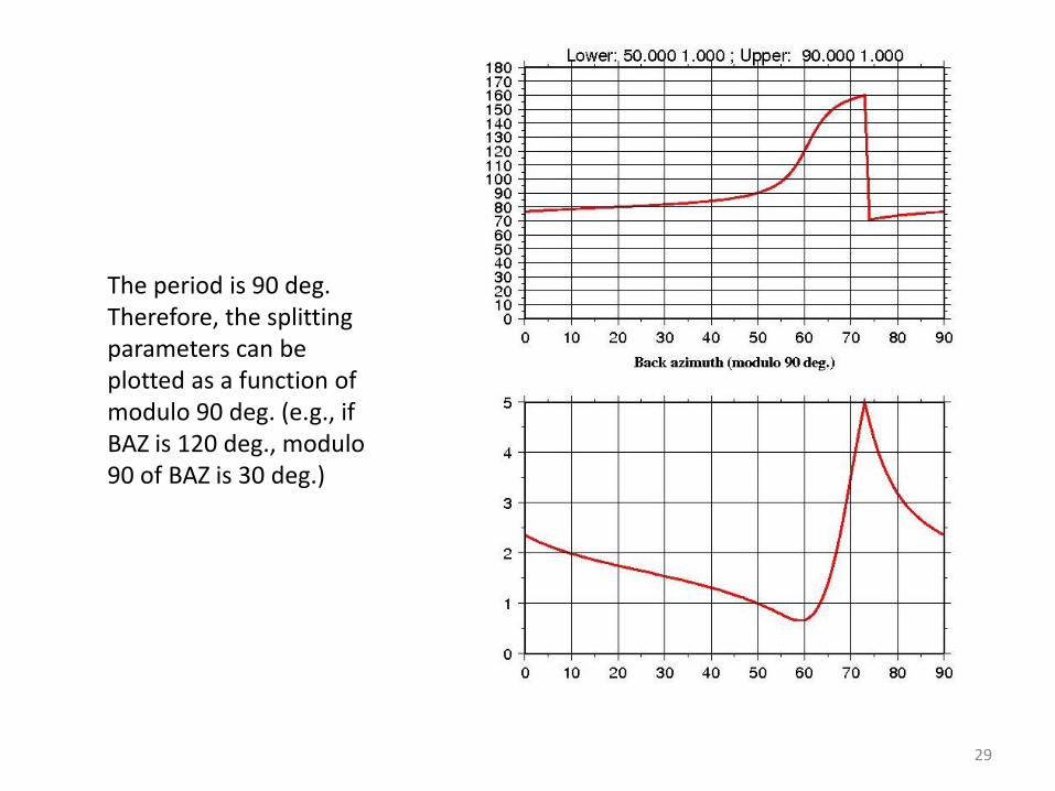
The period is 90 deg. Therefore, the splitting parameters can be plotted as a function of modulo 90 deg. (e.g., if BAZ is 120 deg., modulo 90 of BAZ is 30 deg.)

29

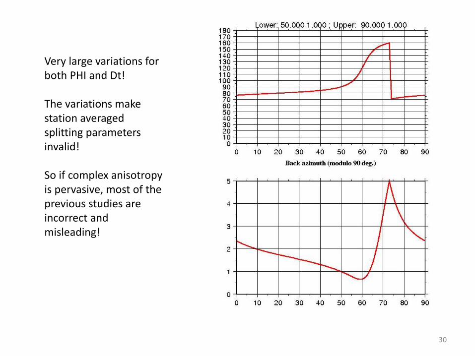
Very large variations for both PHI and Dt! The variations make station averaged splitting parameters invalid! So if complex anisotropy is pervasive, most of the previous studies are incorrect and misleading!

30

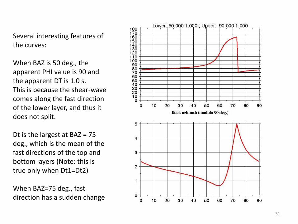
Several interesting features of the curves: When BAZ is 50 deg., the apparent PHI value is 90 and the apparent DT is 1.0 s. This is because the shear-wave comes along the fast direction of the lower layer, and thus it does not split. Dt is the largest at BAZ = 75 deg., which is the mean of the fast directions of the top and bottom layers (Note: this is true only when Dt1=Dt2) When BAZ=75 deg., fast direction has a sudden change

31

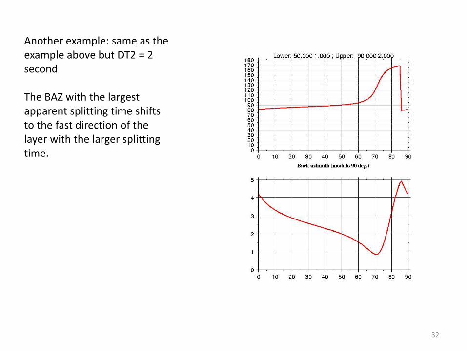
Another example: same as the example above but DT2 = 2 second The BAZ with the largest apparent splitting time shifts to the fast direction of the layer with the larger splitting time.

32

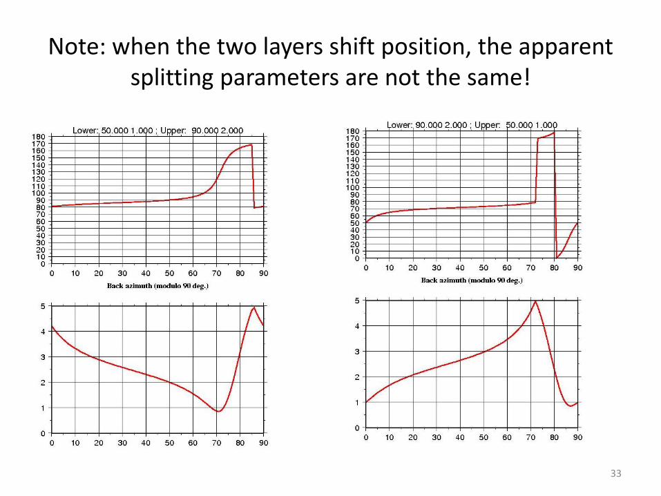
Note: when the two layers shift position, the apparent splitting parameters are not the same!

33

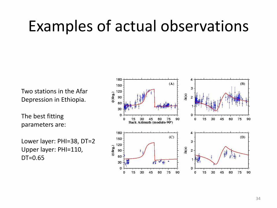
Examples of actual observations

Two stations in the Afar Depression in Ethiopia. The best fitting parameters are: Lower layer: PHI=38, DT=2 Upper layer: PHI=110, DT=0.65

34

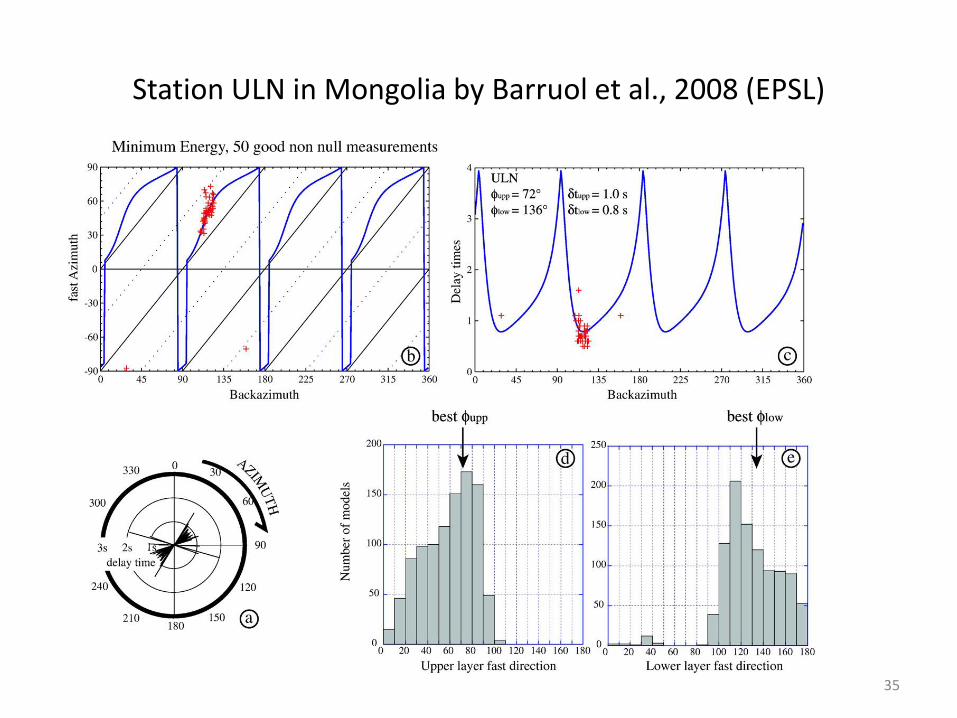
Station ULN in Mongolia by Barruol et al., 2008 (EPSL)

35

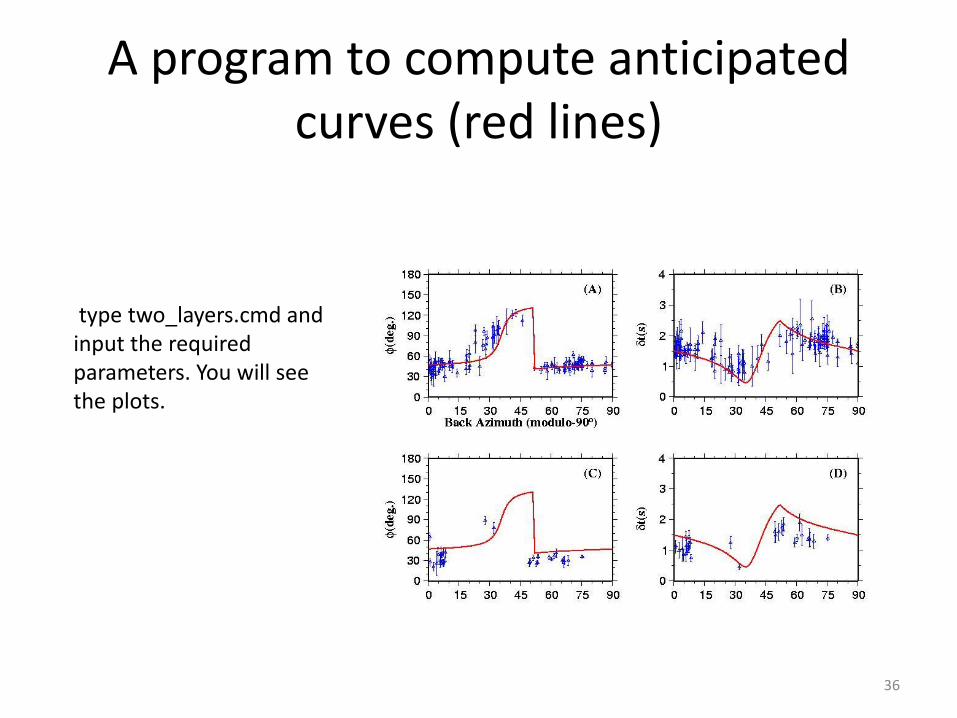
A program to compute anticipated curves (red lines)

type two_layers.cmd and input the required parameters. You will see the plots.

36

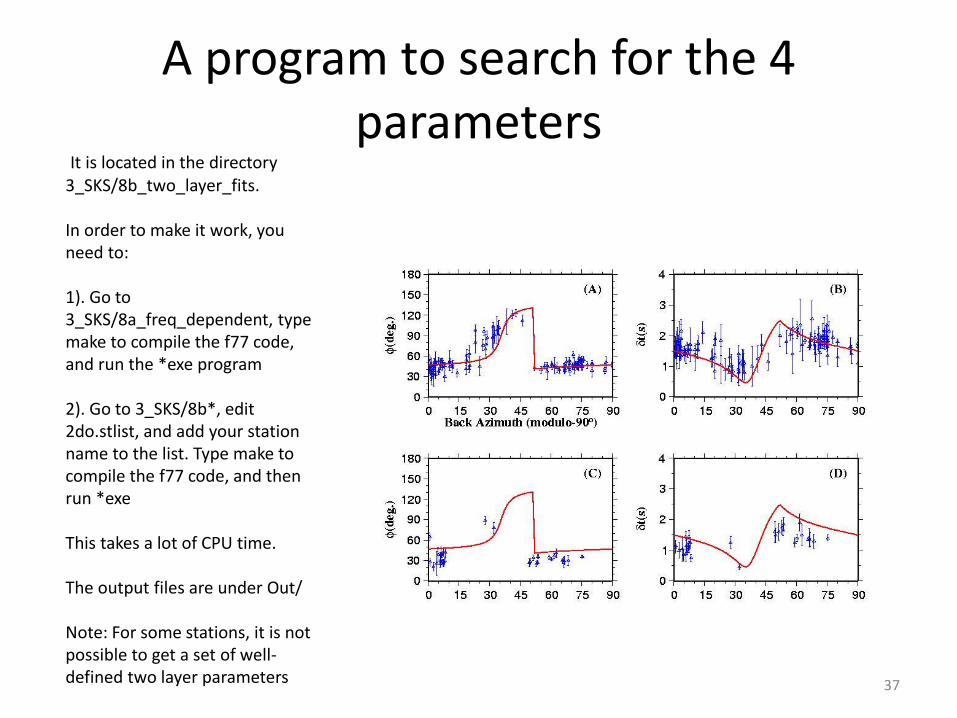
A program to search for the 4 parameters

It is located in the directory 3_SKS/8b_two_layer_fits. In order to make it work, you need to: 1). Go to 3_SKS/8a_freq_dependent, type make to compile the f77 code, and run the *exe program 2). Go to 3_SKS/8b*, edit 2do.stlist, and add your station name to the list. Type make to compile the f77 code, and then run *exe This takes a lot of CPU time. The output files are under Out/ Note: For some stations, it is not possible to get a set of well-defined two layer parameters 37

Other indications of complex anisotropy (see Long and Silver, 2009)

• Frequency-dependent

• Small scale variations

• Obvious differences in the results from different methods

38

Other topics of seismic anisotropy to be mastered if you want to become a world-class “anisotropiest”

• Determining splitting parameters using non-XKS shear-waves such as local S-wave (Liu et al., 2008 JGR), SS wave, ScS wave (Hiramatsu et al., 2009 GJI), teleseismic S-wave, and P-to-S converted wave (McNamara and Owens, 1993 JGR)

• Measuring seismic anisotropy using surface waves (Marone and Romanowicz, 2007 Nature) and P waves (Bokelmann, 2002 GJI)

• Interpret your results to make significant progress toward our understanding of the structure and dynamics of the Earth’s interior. Examples of seismic anisotropy papers published on Nature or Science:

• Gao et al., 1994 (Nature), Kendall et al., 2005 (Nature), Makeyeva et al., 1992 (Nature), Rumpker et al, 2003 (Nature), Wolfe and Solomon, 1998 (Science), Gerst et al., 2004 (Science), Long and Silver, 2008 (Science), Panning et al., 2004 (Science)

39

Possible causes of anisotropy in the Upper mantle

• Lattice preferred orientation (LPO) of olivine crystals

• Vertical magmatic dikes

• LPO of serpentine (in subduction zones only. This is the newest of all – First reported by Katayama et al. in the October, 22, 2009 issue of Nature. Still needs to be confirmed and we will not talk about this in this class)

40

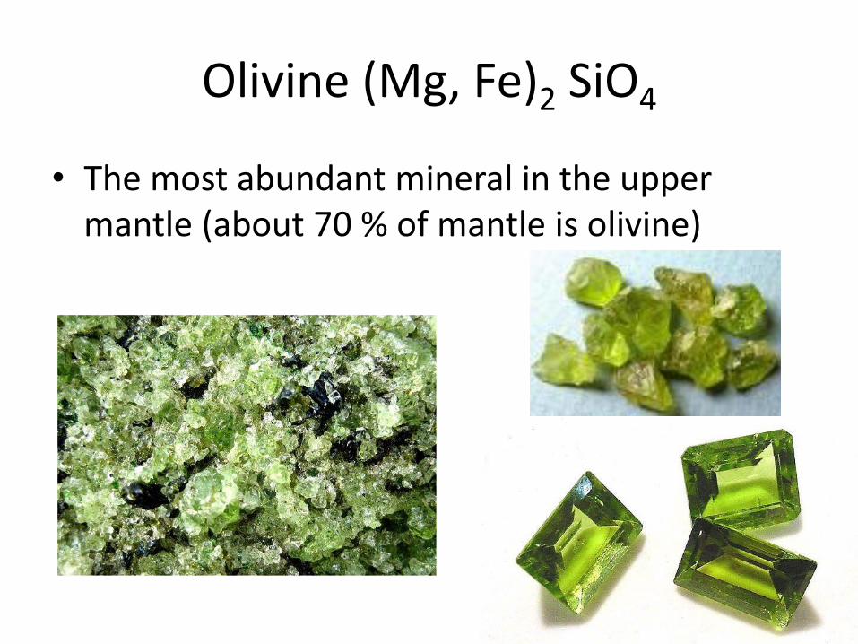
Olivine (Mg, Fe)2 SiO4

• The most abundant mineral in the upper mantle (about 70 % of mantle is olivine)

41

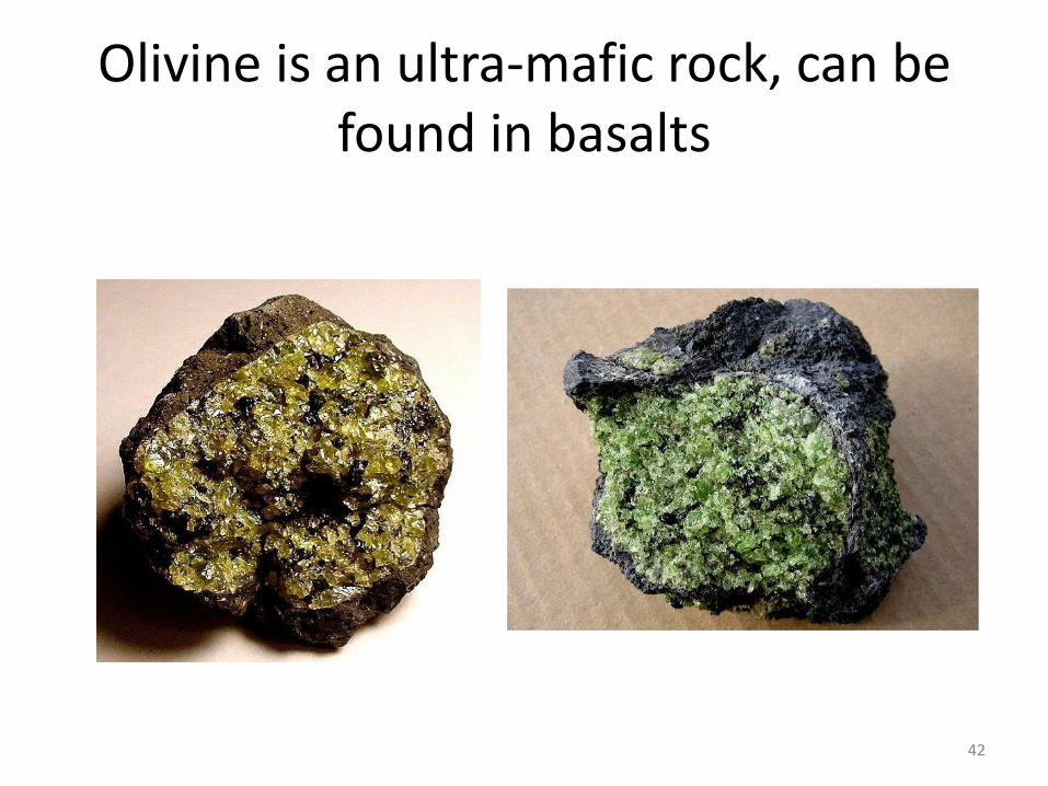
Olivine is an ultra-mafic rock, can be found in basalts

42

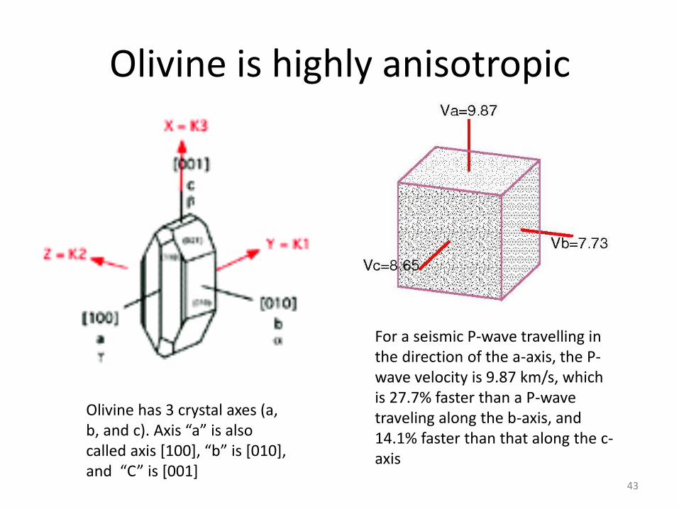
Olivine is highly anisotropic

Olivine has 3 crystal axes (a, b, and c). Axis “a” is also called axis [100], “b” is [010], and “C” is [001]

For a seismic P-wave travelling in the direction of the a-axis, the P-wave velocity is 9.87 km/s, which is 27.7% faster than a P-wave traveling along the b-axis, and 14.1% faster than that along the c-axis

43

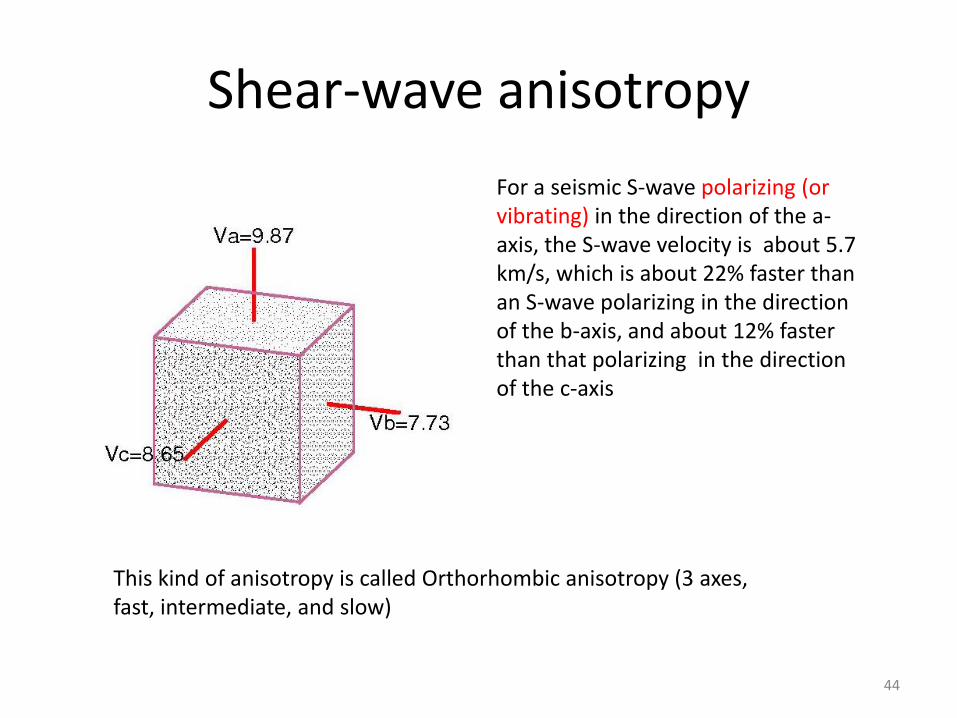
Shear-wave anisotropy

For a seismic S-wave polarizing (or vibrating) in the direction of the a-axis, the S-wave velocity is about 5.7 km/s, which is about 22% faster than an S-wave polarizing in the direction of the b-axis, and about 12% faster than that polarizing in the direction of the c-axis

This kind of anisotropy is called Orthorhombic anisotropy (3 axes, fast, intermediate, and slow)

44

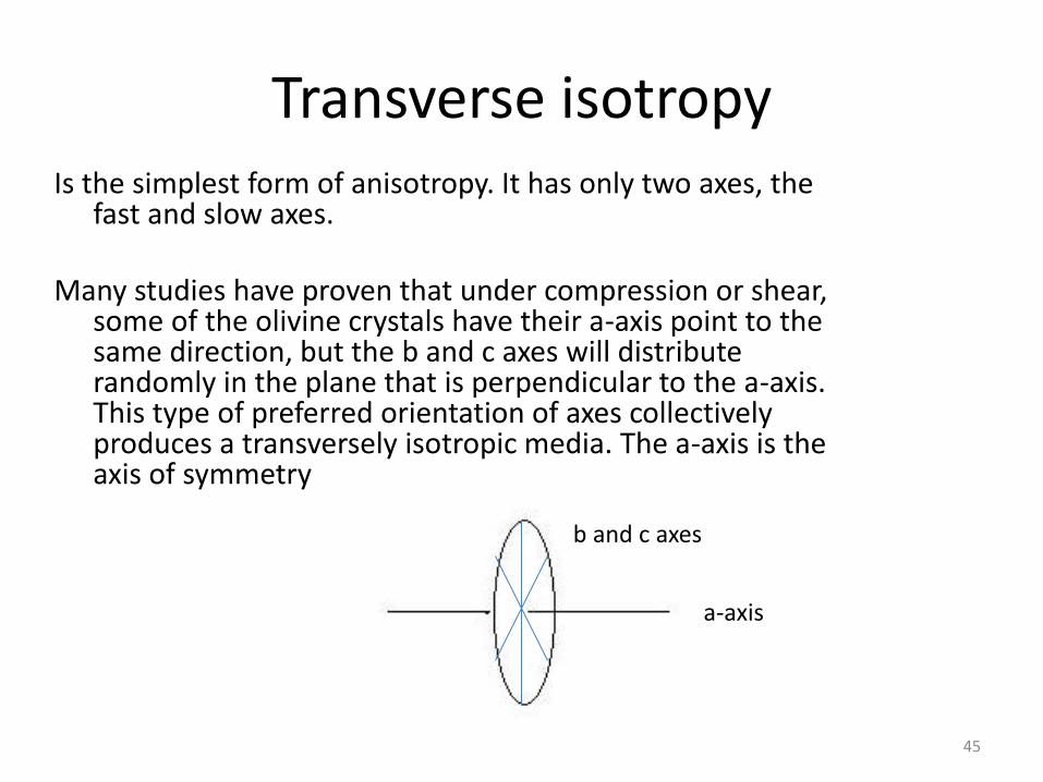
Transverse isotropy Is the simplest form of anisotropy. It has only two axes, the

fast and slow axes. Many studies have proven that under compression or shear,

some of the olivine crystals have their a-axis point to the same direction, but the b and c axes will distribute randomly in the plane that is perpendicular to the a-axis. This type of preferred orientation of axes collectively produces a transversely isotropic media. The a-axis is the axis of symmetry

a-axis

b and c axes

45

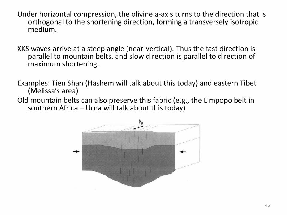
Under horizontal compression, the olivine a-axis turns to the direction that is orthogonal to the shortening direction, forming a transversely isotropic medium.

XKS waves arrive at a steep angle (near-vertical). Thus the fast direction is

parallel to mountain belts, and slow direction is parallel to direction of maximum shortening.

Examples: Tien Shan (Hashem will talk about this today) and eastern Tibet

(Melissa’s area) Old mountain belts can also preserve this fabric (e.g., the Limpopo belt in

southern Africa – Urna will talk about this today)

46

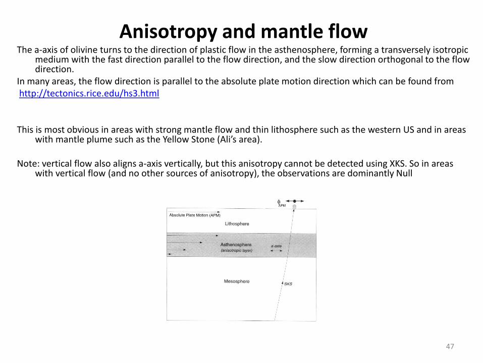
Anisotropy and mantle flow The a-axis of olivine turns to the direction of plastic flow in the asthenosphere, forming a transversely isotropic

medium with the fast direction parallel to the flow direction, and the slow direction orthogonal to the flow direction.

In many areas, the flow direction is parallel to the absolute plate motion direction which can be found from http://tectonics.rice.edu/hs3.html This is most obvious in areas with strong mantle flow and thin lithosphere such as the western US and in areas

with mantle plume such as the Yellow Stone (Ali’s area). Note: vertical flow also aligns a-axis vertically, but this anisotropy cannot be detected using XKS. So in areas

with vertical flow (and no other sources of anisotropy), the observations are dominantly Null

47

Wikipedia Definition of Viscosity

• Viscosity describes a fluid's internal resistance to flow and may be thought of as a measure of fluid friction. For example, high-viscosity felsic magma will create a tall, steep stratovolcano, because it cannot flow far before it cools, while low-viscosity mafic lava will create a wide, shallow-sloped shield volcano.

48

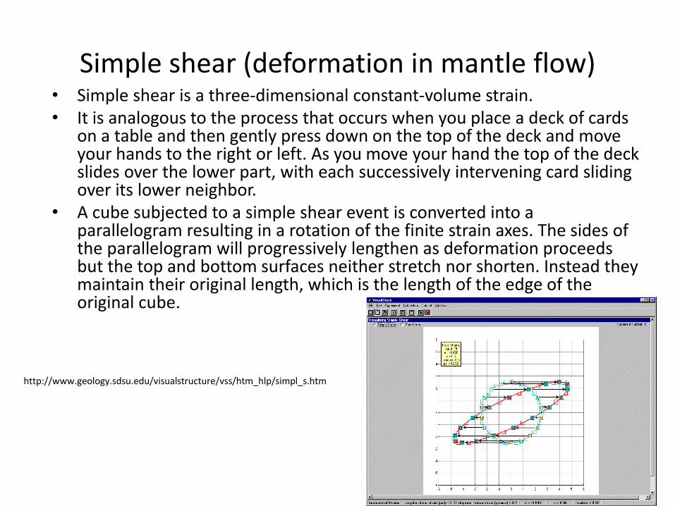
Simple shear (deformation in mantle flow) • Simple shear is a three-dimensional constant-volume strain. • It is analogous to the process that occurs when you place a deck of cards

on a table and then gently press down on the top of the deck and move your hands to the right or left. As you move your hand the top of the deck slides over the lower part, with each successively intervening card sliding over its lower neighbor.

• A cube subjected to a simple shear event is converted into a parallelogram resulting in a rotation of the finite strain axes. The sides of the parallelogram will progressively lengthen as deformation proceeds but the top and bottom surfaces neither stretch nor shorten. Instead they maintain their original length, which is the length of the edge of the original cube.

49

http://www.geology.sdsu.edu/visualstructure/vss/htm_hlp/simpl_s.htm

Newtonian fluid

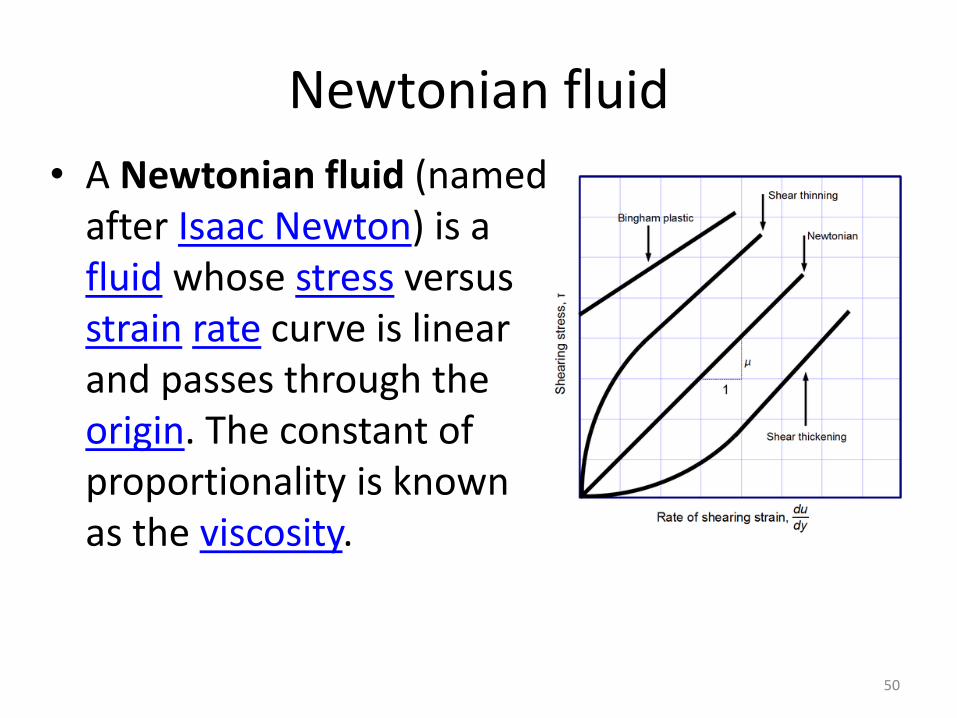
• A Newtonian fluid (named after Isaac Newton) is a fluid whose stress versus strain rate curve is linear and passes through the origin. The constant of proportionality is known as the viscosity.

50

Lithosphere westward drift and the no-net-rotation reference frame

• NNR frame assumes that the Earth’s lithosphere as a whole is fixed relative to the deep mantle, and all the plate motions are relative to each other. Analogy: moving ice sheets in a still lake.

• Net rotation: The lithosphere as a whole is moving. Most studies found that it is moving toward the west around a pole in the southern Indian ocean. Analogy: moving ice sheets in a flowing river. For North America, this net rotation is about 2 cm/yr toward the SW. The absolute plate motion (APM) model of Gripp and Gordon (2002) that we commonly use considers both NNR and net rotation.

51

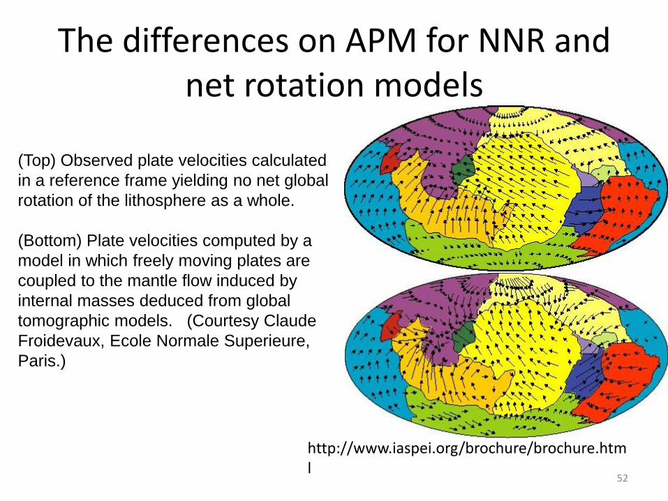
The differences on APM for NNR and net rotation models

(Top) Observed plate velocities calculated

in a reference frame yielding no net global

rotation of the lithosphere as a whole.

(Bottom) Plate velocities computed by a

model in which freely moving plates are

coupled to the mantle flow induced by

internal masses deduced from global

tomographic models. (Courtesy Claude

Froidevaux, Ecole Normale Superieure,

Paris.)

http://www.iaspei.org/brochure/brochure.html

52

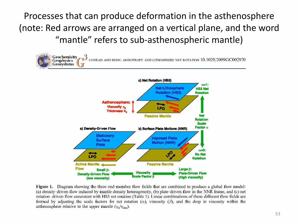
Processes that can produce deformation in the asthenosphere (note: Red arrows are arranged on a vertical plane, and the word

“mantle” refers to sub-asthenospheric mantle)

53

Some terms

• ISA – Infinite strain axis

• A-type fabric of olivine

• Other types of olivine fabrics

• LPO-Lattice preferred orientation

• Dislocation creep

54

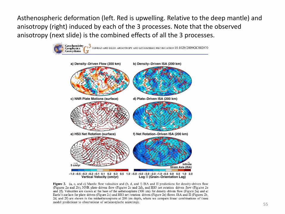
Asthenospheric deformation (left. Red is upwelling. Relative to the deep mantle) and anisotropy (right) induced by each of the 3 processes. Note that the observed anisotropy (next slide) is the combined effects of all the 3 processes.

55

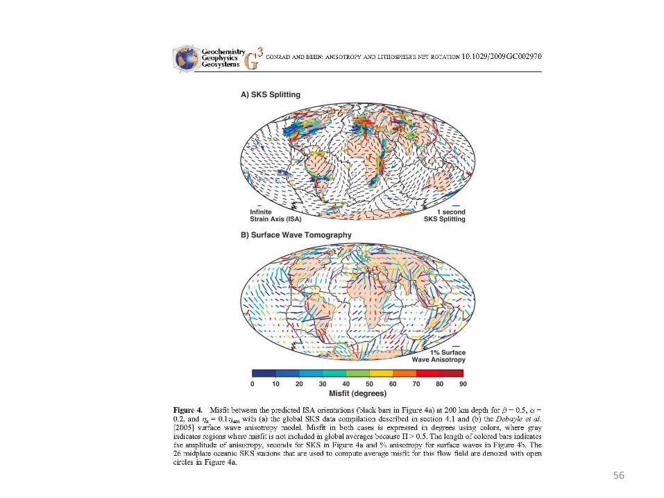
56

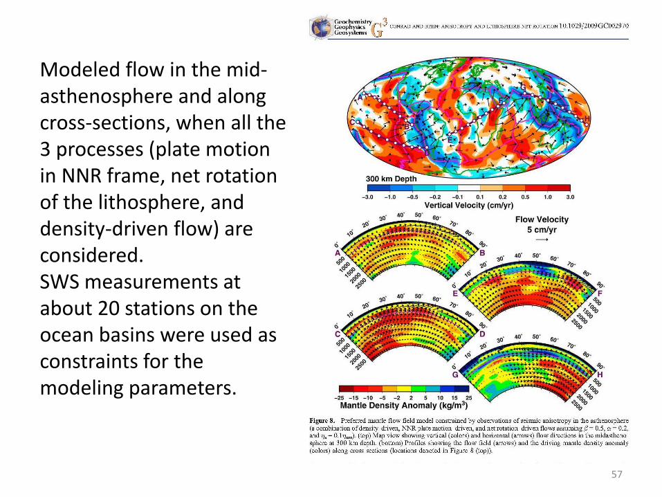
Modeled flow in the mid-asthenosphere and along cross-sections, when all the 3 processes (plate motion in NNR frame, net rotation of the lithosphere, and density-driven flow) are considered. SWS measurements at about 20 stations on the ocean basins were used as constraints for the modeling parameters.

57

58

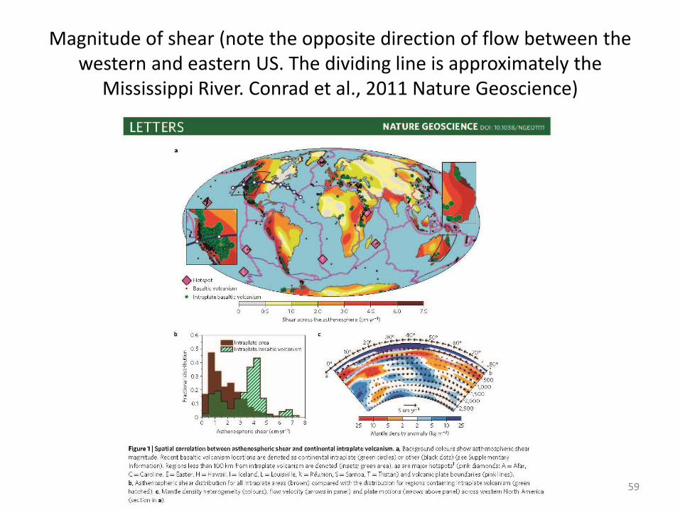
Magnitude of shear (note the opposite direction of flow between the western and eastern US. The dividing line is approximately the

Mississippi River. Conrad et al., 2011 Nature Geoscience)

59

60

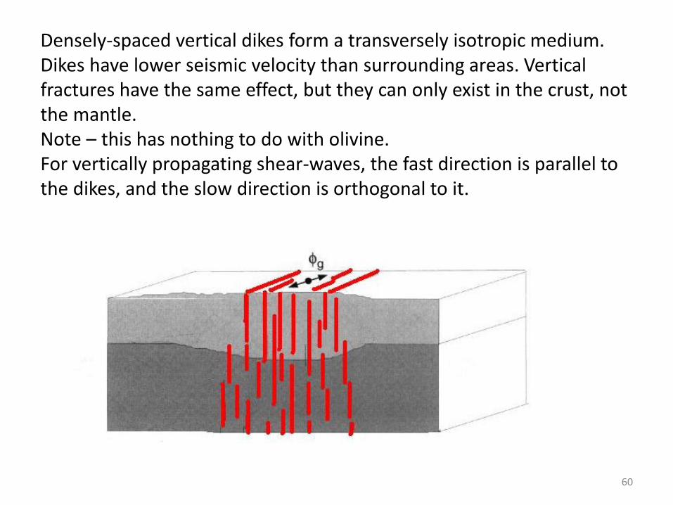
Densely-spaced vertical dikes form a transversely isotropic medium. Dikes have lower seismic velocity than surrounding areas. Vertical fractures have the same effect, but they can only exist in the crust, not the mantle. Note – this has nothing to do with olivine. For vertically propagating shear-waves, the fast direction is parallel to the dikes, and the slow direction is orthogonal to it.

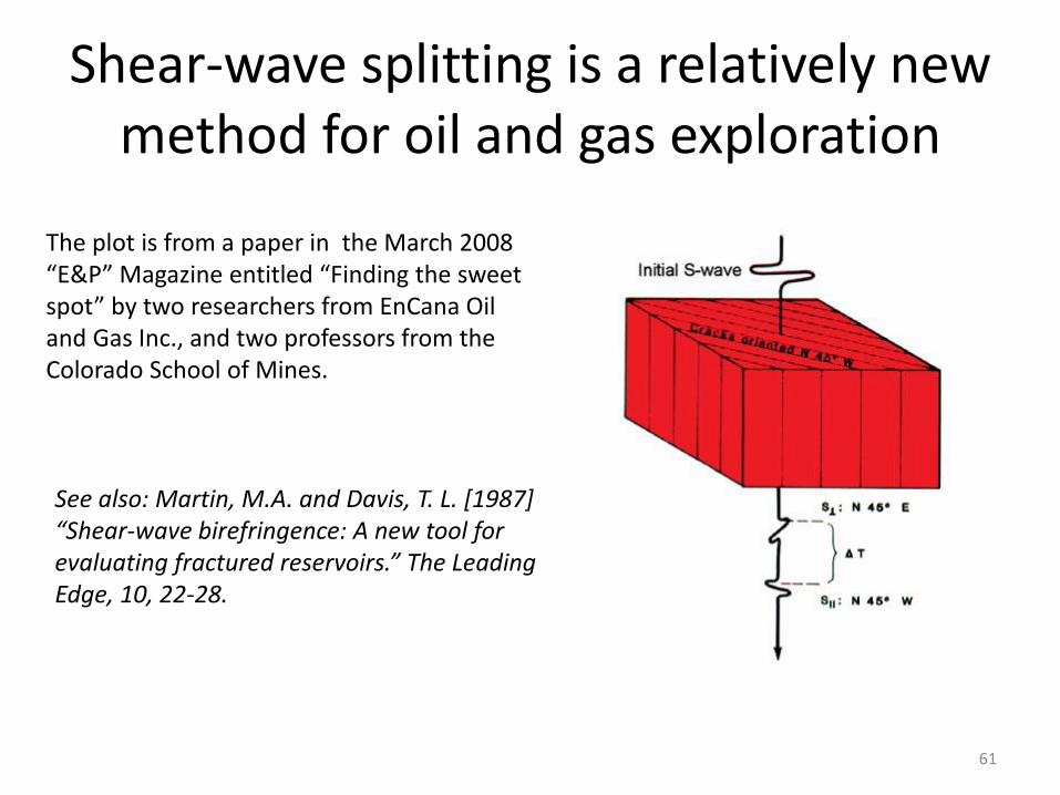
Shear-wave splitting is a relatively new method for oil and gas exploration

The plot is from a paper in the March 2008 “E&P” Magazine entitled “Finding the sweet spot” by two researchers from EnCana Oil and Gas Inc., and two professors from the Colorado School of Mines.

See also: Martin, M.A. and Davis, T. L. [1987] “Shear-wave birefringence: A new tool for evaluating fractured reservoirs.” The Leading Edge, 10, 22-28.

61

Remarks on more advanced interpretation of seismic anisotropy

• For a given area, one, two, or all the three of the mechanisms (flow, compression, dikes) can exist. If the fast directions are different, this combination leads to complex anisotropy (characterized by variation of splitting parameters with azimuths). Further readings on this subject: Gao and Liu, 2009 (G-cubed).

• The a-axis can tilt, and the dikes may not be vertical. These also lead to complex anisotropy. Confirmed studies of this type are rare.

• In areas with a lot of water in the mantle (e.g., subduction zones), the a-axis might not align with the flow direction and could even be orthogonal to flow direction (see Karato et al., 2008: Geodynamic significance of seismic anisotropy of the Upper mantle. Annual reviews of Earth and Planetary Science, 2008, page 59-95.

• Receiver function stacking to study the Earth’s crust

62