1

SEGMENTATION OF HUMAN FACIAL MUSCLES ON CT AND MRI DATA USINGLEVEL SET AND BAYESIAN METHODS

A THESIS SUBMITTED TOTHE GRADUATE SCHOOL OF INFORMATICS

OFTHE MIDDLE EAST TECHNICAL UNIVERSITY

BY

HIKMET EMRE KALE

IN PARTIAL FULFILLMENT OF THE REQUIREMENTS FOR THE DEGREE OFMASTER OF SCIENCE

INTHE DEPARTMENT OF HEALTH INFORMATICS

JUNE 2011

Approval of the Graduate School of Informatics

Prof. Dr. Nazife BAYKAL

Director

I certify that this thesis satisfies all the requirements as a thesis for the degree of Master of

Science.

Assist. Prof. Dr. Didem GOKCAY

Head of Department

This is to certify that we have read this thesis and that in our opinion it is fully adequate, in

scope and quality, as a thesis for the degree of Master of Science.

Assoc. Prof. Dr. Erkan MUMCUOGLU

Supervisor

Examining Committee Members

Prof. Dr. Fatos Tunay YARMAN VURAL (METU, CENG)

Assoc. Prof. Dr. U. Erkan MUMCUOGLU (METU, II)

Assist. Prof. Dr. Didem GOKCAY (METU, II)

Assist. Prof. Dr. Alptekin TEMIZEL (METU, II)

Prof. Dr. Yasemin YARDIMCI (METU, II)

I hereby declare that all information in this document has been obtained and presentedin accordance with academic rules and ethical conduct. I also declare that, as requiredby these rules and conduct, I have fully cited and referenced all material and results thatare not original to this work.

Name, Last Name: Hikmet Emre Kale

Signature :

iii

ABSTRACT

SEGMENTATION OF HUMAN FACIAL MUSCLES ON CT AND MRI DATA USINGLEVEL SET AND BAYESIAN METHODS

Kale, Hikmet Emre

M.S., Department of Health Informatics

Supervisor : Assoc. Prof. Dr. Erkan MUMCUOGLU

June 2011, 77 pages

Medical image segmentation is a challenging problem, and is studied widely. In this the-

sis, the main goal is to develop automatic segmentation techniques of human mimic muscles

and to compare them with ground truth data in order to determine the method that provides

best segmentation results. The segmentation methods are based on Bayesian with Markov

Random Field (MRF) and Level Set (Active Contour) models. Proposed segmentation meth-

ods are multi step processes including preprocess, main muscle segmentation step and post

process, and are applied on three types of data: Magnetic Resonance Imaging (MRI) data,

Computerized Tomography (CT) data and unified data, in which case, information coming

from both modalities are utilized. The methods are applied both in three dimensions (3D) and

two dimensions (2D) data cases. A simulation data and two patient data are utilized for tests.

The patient data results are compared statistically with ground truth data which was labeled

by an expert radiologist.

Keywords: Medical Image Segmentation, Level Sets, Bayesian Methods, Markov Random

Fields

iv

OZ

INSAN YUZ KASLARININ KESIT KUMESI VE BAYESCI YONTEMLERLEMANYETIK REZONANS VE BILGISAYARLI TOMOGRAFI VERISI

KULLANILARAK BOLUTLENMESI

Kale, Hikmet Emre

Yuksek Lisans, Saglık Bilisimi Bolumu

Tez Yoneticisi : Doc. Dr. Erkan MUMCUOGLU

Haziran 2011, 77 sayfa

Tıbbi goruntu bolutleme pek cok zorluklar icerir ve uzerinde sıklıkla calısılan bir problemdir.

Bu tezin ana hedefi insan mimik kaslarını otomatik olarak bolutlemek icin yontemler gelistirmek

ve bu yontemleri karsılastırarak en iyi yontemi belirlemektir. Bolutleme yontemleri Bayesci

Markov Rastgele Alanlar ve Etkin Cevre Hatları modelleri uzerine kurulmustur. Onerilen

bolutleme yontemleri on isleme, ana kas bolutleme islemi ve son islem kısımlarını iceren

birden cok basamaklı birer islemdir. Yontemler Manyetik Rezonans (MR), Bilgisayarlı To-

mografi (BT) verisi ve bilginin her iki veriden de geldigi birlestirilmis veri seti uzerinde

uygulandı. Yontemler hem iki boyutlu hem uc boyutlu olarak uygulandı. Hasta verisin-

den elde edilen sonuclar uzman bir radyolog tarafından isaretlenmis kaslarla istatistiki olarak

karsılastırıldı.

Anahtar Kelimeler: Tıbbi Goruntu Bolutleme, Kesit Kumesi Yontemi, Bayesci Yontemler,

Markov Rastgele Alanlar

v

To My Family

vi

ACKNOWLEDGMENTS

I express sincere appreciation to my supervisor Assoc. Prof. Dr. Erkan Mumcuoglu for his

patience guidance throughout the research. I greatly appreciate his share in every step in the

development of the thesis.

Thanks go to Dr. Salih Hamcan for labeling images for the ground truth data and Dr. Fatih

Ors for providing MR and CT images.

I am deeply grateful to my friend Emre Sener for sharing his knowledge and for his guidance

during the Tubitak 1001 Project and this thesis.

I would also gratefully thank to my parents, my father Cahit Kale and my mother Suheyla

Kale -to whom i owe everything- for their patience in this long M.S. period, for their support

in all kind of manner and for making my life easier. Their insight and support always helped

me a lot.

I would also like to thank to my brother, Enderay Kale for supporting and motivating me. I

am grateful that he always listens to me patiently and gives wise advices to me.

My friends, Ferit Uzer and Mehmet Akif Antepli’s helps while editing the thesis and their

support are also gratefully appreciated.

I also thank to my friend Ilker Kocamıs, with whom we have grown up together and share

many things with each other, for motivating me.

vii

TABLE OF CONTENTS

ABSTRACT . . . . . . . . . . . . . . . . . . . . . . . . . . . . . . . . . . . . . . . . iv

OZ . . . . . . . . . . . . . . . . . . . . . . . . . . . . . . . . . . . . . . . . . . . . . v

DEDICATON . . . . . . . . . . . . . . . . . . . . . . . . . . . . . . . . . . . . . . . vi

ACKNOWLEDGMENTS . . . . . . . . . . . . . . . . . . . . . . . . . . . . . . . . . vii

TABLE OF CONTENTS . . . . . . . . . . . . . . . . . . . . . . . . . . . . . . . . . viii

LIST OF TABLES . . . . . . . . . . . . . . . . . . . . . . . . . . . . . . . . . . . . xi

LIST OF FIGURES . . . . . . . . . . . . . . . . . . . . . . . . . . . . . . . . . . . . xii

LIST OF ABBREVIATIONS . . . . . . . . . . . . . . . . . . . . . . . . . . . . . . . xv

CHAPTERS

1 INTRODUCTION . . . . . . . . . . . . . . . . . . . . . . . . . . . . . . . 1

1.1 Scope and Motivation . . . . . . . . . . . . . . . . . . . . . . . . . 1

1.2 Image Segmentation . . . . . . . . . . . . . . . . . . . . . . . . . . 2

1.3 Source of Data . . . . . . . . . . . . . . . . . . . . . . . . . . . . . 4

1.4 Contributions . . . . . . . . . . . . . . . . . . . . . . . . . . . . . 5

1.5 Organization of the thesis . . . . . . . . . . . . . . . . . . . . . . . 6

2 LEVEL SET AND BAYESIAN MARKOV RANDOM FIELD SEGMENTA-TION . . . . . . . . . . . . . . . . . . . . . . . . . . . . . . . . . . . . . . 7

2.1 Level Set Segmentation . . . . . . . . . . . . . . . . . . . . . . . . 7

2.1.1 Motion in an Externally Generated Velocity Field . . . . . 9

2.1.2 Hamilton-Jacobi Equations . . . . . . . . . . . . . . . . . 15

2.1.3 Motion in Normal Direction . . . . . . . . . . . . . . . . 16

2.1.4 Curvature Evolution . . . . . . . . . . . . . . . . . . . . 17

2.2 Geometric Integral Measures . . . . . . . . . . . . . . . . . . . . . 19

viii

2.2.1 Geodesic Active Contours, Surfaces . . . . . . . . . . . . 20

2.2.2 Minimum Variance . . . . . . . . . . . . . . . . . . . . . 22

2.3 Level Set Segmentation Model . . . . . . . . . . . . . . . . . . . . 23

2.3.1 Preprocess . . . . . . . . . . . . . . . . . . . . . . . . . . 24

2.3.2 Main Part . . . . . . . . . . . . . . . . . . . . . . . . . . 26

2.3.3 Postprocess . . . . . . . . . . . . . . . . . . . . . . . . . 30

2.4 A Bayesian Markov Random Field Segmentation Using a Partial Vol-ume Model . . . . . . . . . . . . . . . . . . . . . . . . . . . . . . . 32

2.4.1 Adaptive Bayesian Segmentation Model . . . . . . . . . . 35

3 SIMULATION AND PATIENT DATA . . . . . . . . . . . . . . . . . . . . . 37

3.1 Simulation . . . . . . . . . . . . . . . . . . . . . . . . . . . . . . . 37

3.1.1 Metrics . . . . . . . . . . . . . . . . . . . . . . . . . . . 38

3.1.2 Parameter Optimization . . . . . . . . . . . . . . . . . . . 39

3.2 Ground Truth of Patient Data . . . . . . . . . . . . . . . . . . . . . 40

4 RESULTS . . . . . . . . . . . . . . . . . . . . . . . . . . . . . . . . . . . . 42

4.1 Metrics and Statistical Analysis . . . . . . . . . . . . . . . . . . . . 42

4.2 Comparison of Methods . . . . . . . . . . . . . . . . . . . . . . . . 43

4.2.1 Bayesian with MRF Model Results . . . . . . . . . . . . 43

4.2.2 Level Set Model Results . . . . . . . . . . . . . . . . . . 49

5 CONCLUSIONS AND FUTURE WORK . . . . . . . . . . . . . . . . . . . 54

5.1 Conclusion and Discussion . . . . . . . . . . . . . . . . . . . . . . 54

5.2 Future Work . . . . . . . . . . . . . . . . . . . . . . . . . . . . . . 56

REFERENCES . . . . . . . . . . . . . . . . . . . . . . . . . . . . . . . . . . . . . . 57

APPENDICES

A PROPERTIES OF RADIOLOGICAL DATA AND ACQUISITION PARAM-ETERS . . . . . . . . . . . . . . . . . . . . . . . . . . . . . . . . . . . . . 61

B FORMAL DEFINITION OF LEVEL SET EQUATION . . . . . . . . . . . . 63

C FIRST, SECOND AND THIRD ORDER HAMILTON-JACOBI NON OS-CILLATORY NUMERICAL SCHEMES FOR SPATIAL DERIVATIVE . . . 65

C.1 Interpolation Using Newton’s Divided Difference Polynomial . . . . 65

C.2 First, Second and Third order Essentially Non-Oscillator Schemes . 66

ix

D MEAN CURVATURE OF 3D AND 4D IMPLICIT FUNCTION . . . . . . . 69

E GEODESIC ACTIVE CONTOURS . . . . . . . . . . . . . . . . . . . . . . 70

F MINIMUM VARIANCE TERM . . . . . . . . . . . . . . . . . . . . . . . . 73

G BACKWARD EULER TIME SOLUTION OF CURVATURE LIKE FORCESIN LEVEL SET EQUATIONS . . . . . . . . . . . . . . . . . . . . . . . . . 76

x

LIST OF TABLES

Table 2.1 The spatial derivative choices of Godunov Scheme, ϕ is the level set function

and subscripts x and y are to represent partial derivatives. F is a scalar on the

coordinates (x, y) . . . . . . . . . . . . . . . . . . . . . . . . . . . . . . . . . . . 17

Table 4.1 p values for paired t-tests for Bayesian methods with RVFBI applied to

MR&CT unified data. Every p is greater than α = 0.05, which means that are

statistically not different from each other. . . . . . . . . . . . . . . . . . . . . . . 48

Table 4.2 Run times (sec) for the methods. Measurements are for 40 iterations of

Level Set method and for one iteration of Bayesian method. Single refers to CT

or MR only data case and Unified refers to MR&CT case. . . . . . . . . . . . . . 52

xi

LIST OF FIGURES

Figure 2.1 Implicit Surface (ϕ) and its zero level set shown by red contour. (a) Side

view (b) Upper view (Projection to the x-y plane) . . . . . . . . . . . . . . . . . 8

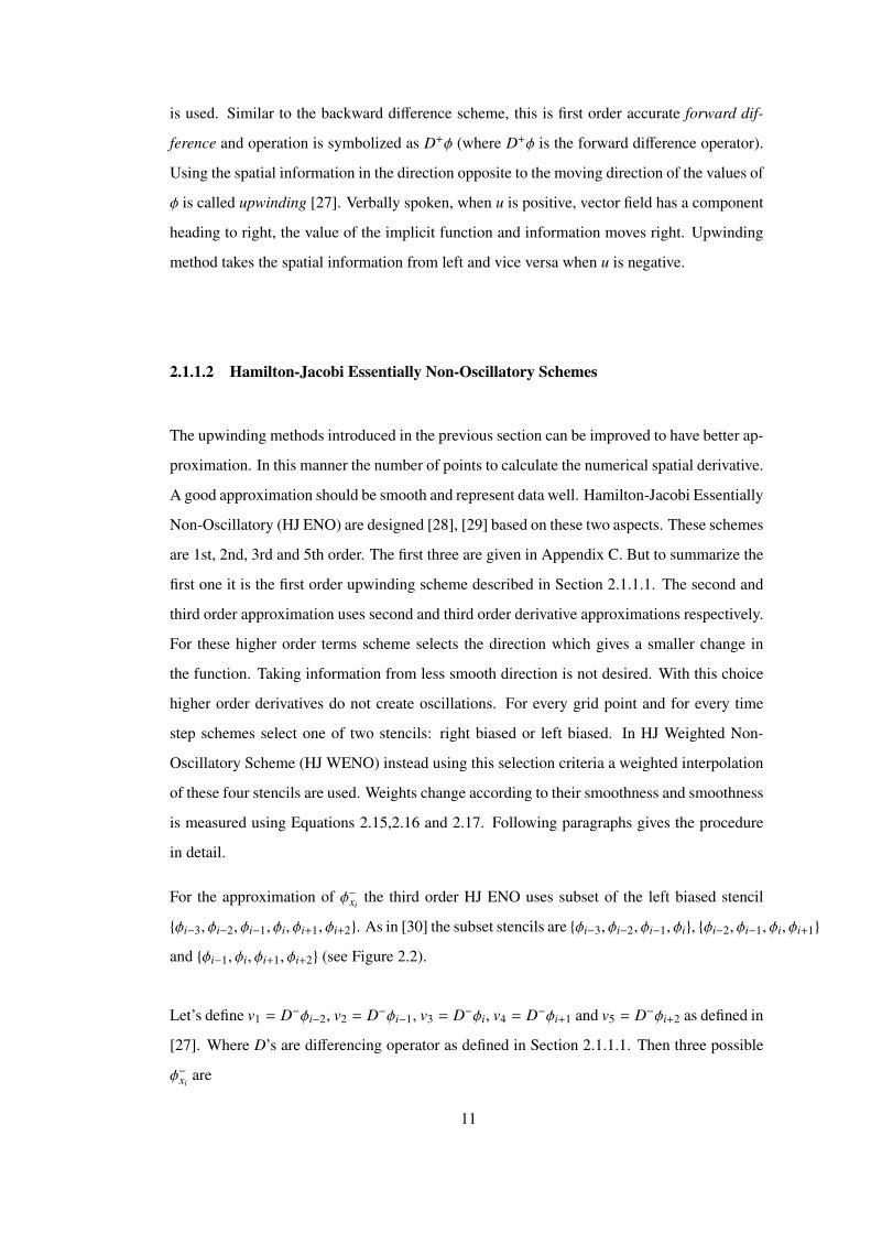
Figure 2.2 Three subsets of the stencil: (a) Left biased stencil to calculate ϕ−xi(b) Right

biased stencil to calculate ϕ+xi. . . . . . . . . . . . . . . . . . . . . . . . . . . . 12

Figure 2.3 Curvature directions on the boundary . . . . . . . . . . . . . . . . . . . . 19

Figure 2.4 Curvature motion of a star shaped curve . . . . . . . . . . . . . . . . . . . 20

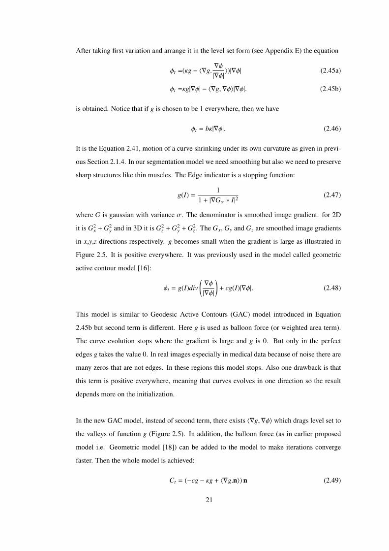
Figure 2.5 1D illustration of the GAC model, (a) I vs x, An edge in an image(I) (b)

∇Gσ ∗ I vs x, smoothed version of (a). (c) Edge indicator function g and directions

of the curve through the valleys . . . . . . . . . . . . . . . . . . . . . . . . . . . 22

Figure 2.6 Standard Level Set (Forward Euler) Segmentation Method . . . . . . . . . 25

Figure 2.7 Forward Euler Time Level Set Algorithm . . . . . . . . . . . . . . . . . . 28

Figure 2.8 Backward Euler Time Level Set Algorithm . . . . . . . . . . . . . . . . . 29

Figure 2.9 Thickness Adaptive Level Set (Forward Euler) Segmentation Method . . . 31

Figure 2.10 Standard Bayesian Segmentation Method . . . . . . . . . . . . . . . . . . 34

Figure 2.11 Adaptive Bayesian Segmentation Method . . . . . . . . . . . . . . . . . . 36

Figure 3.1 Steps of creating synthetic MR and CT images . . . . . . . . . . . . . . . 38

Figure 3.2 Screen shot of the software program ITK Snap v 2.0. A CT volume is

labeled. Red color is for Bone, Green is for Muscle and Blue is for Skin. Upper

Left: axial view; upper right: sagittal view and lower right coronal view. . . . . . 40

Figure 4.1 Mean (Dice, RMSSSD) ± Standard deviation plot of metrics for 16 ROI’s

for 8 Bayesian methods applied to MR data (a) Dice Coefficients vs Methods. (b)

RMSSSD vs Methods. ‘Y’: with RVFBI,‘N’: w/o RVFBI, Standard: Standard

Bayesian with MRF, Adaptive: Thickness Adaptive Bayesian MRF, ‘3D’: Three

dimensions,‘2D’: Two dimensions. . . . . . . . . . . . . . . . . . . . . . . . . . 44

xii

Figure 4.2 (a) Original MRI Slice, (b) Its ground truth labels (c)3D Bayesian Method

Without RVFBI, Note that the facia in the red rectangle is segmented as air. (d)3D

Bayesian Method with RVFBI. The muscle voxels are removed because of RVFBI.

Green is Muscle, Red is Bone, Blue is Skin, Black is Air and Non-labeled regions

are Fat and Yellow designates soft tissue where intensity is close to Muscle . . . . 45

Figure 4.3 Mean (Dice, RMSSSD) ± Standard deviation plot of metrics for 16 ROI’s

for 8 Bayesian methods applied to CT data (a) Dice Coefficients vs Methods. (b)

RMSSSD vs Methods. . . . . . . . . . . . . . . . . . . . . . . . . . . . . . . . . 46

Figure 4.4 Mean (Dice, RMSSSD) ± Standard deviation plot of metrics for 16 ROI’s

for 8 Bayesian methods applied to MR&CT data (a) Dice Coefficients vs Methods.

(b) RMSSSD vs Methods. . . . . . . . . . . . . . . . . . . . . . . . . . . . . . . 47

Figure 4.5 Bayesian Metrics of best methods of three groups (MR only, CT only and

MR&CT case) vs ROI’s. (a) Dice Coefficients vs ROI’s. (b) RMSSSD graph vs

ROI’s. . . . . . . . . . . . . . . . . . . . . . . . . . . . . . . . . . . . . . . . . 48

Figure 4.6 Mean (Dice, RMSSSD) ± Standard deviation plot of metrics for 16 ROI’s

for 8 Bayesian methods applied to MR data (a) Dice Coefficients vs Methods.

(b) RMSSSD vs Methods. ‘Y’: with RVFBI,‘N’: w/o RVFBI, Standard-p: Stan-

dard LS (FE) with predefined class means, Standard-a: Standard LS (FE) with

automatic class means Adaptive: Thickness Adaptive LS FE,‘3D’: Three dimen-

sions,‘2D’: Two dimensions. . . . . . . . . . . . . . . . . . . . . . . . . . . . . 49

Figure 4.7 Mean (Dice, RMSSSD) ± Standard deviation plot of metrics for 16 ROI’s

for 8 Bayesian methods applied to MR&CT data (a) Dice Coefficients vs Methods.

(b) RMSSSD vs Methods. . . . . . . . . . . . . . . . . . . . . . . . . . . . . . . 50

Figure 4.8 Mean metrics (Dice, RMSSSD) ± Standard deviation plot of metrics for 16

ROI’s for 12 Level Set methods applied to CT only data. (a) Dice Coefficients vs

Methods. (b) RMSSSD vs Methods. . . . . . . . . . . . . . . . . . . . . . . . . 50

Figure 4.9 Level Set Metrics of best methods of three groups (MR only, CT only and

MR&CT case) vs ROI’s. (a) Dice Coefficients vs ROI’s. (b) RMSSSD graph vs

ROI’s. . . . . . . . . . . . . . . . . . . . . . . . . . . . . . . . . . . . . . . . . 51

Figure 4.10 The best of Level Set and Bayesian. (a) Dice Coefficients vs ROI’s. (b)

RMSSSD graph vs ROI’s. . . . . . . . . . . . . . . . . . . . . . . . . . . . . . . 52

xiii

Figure G.1 Lexicographical ordering of an 2D matrix . . . . . . . . . . . . . . . . . . 77

xiv

LIST OF ABBREVIATIONS

2D Two Dimensional

3D Three Dimensional

4D Four Dimensional

Adaptive Thickness adaptive model

ANN Artificial Neural Network

CAD Computer Aided Diagnosis

CFL Courant-Freidreichs-Lewy

CT Computerized Tomography

DC Dice Coefficient

ENO Essentially Non-Oscillatory

FE Forward Euler

GAC Geodesic Active Contour

GATA Gulhane Askeri Tıp Akademisi

HJ Hamilton-Jacobi

HJ ENO Hamilton-Jacobi Essentially Non-Oscillatory Schemes

HJ WENO Hamilton-Jacobian Weighted Essentially Non-Oscillatory Scheme

HU Hounsfield Units

ICM Iterated Conditional Model

kNN k Nearest Neighbors

LS Level Set

xv

MAP Maximum Aposteriori

METU Middle East Technical University

ML Maximum Likelihood

MR Magnetic Resonance

MRF Markov Random Field

MRI Magnetic Resonance Imaging

N No

PV Partial Volume

RMSSSD Root Mean Squared Symmetric Surface Distance

ROI Region of Interest

RVFBI Removing Voxels on the Fat Bone Interface

Standard-a Standard Level Set model with automatically calculated class

means

Standard-p Standard Level Set model with predefine class means

SVM Support Vector Machine

TUBITAK Turkiye Bilimsel ve Teknolojik Arastırma Kurumu

WENO Weighted Essentially Non-Oscillatory

Y Yes

xvi

CHAPTER 1

INTRODUCTION

1.1 Scope and Motivation

In this thesis, the main objective is to develop automatic segmentation methods to segment

the muscles in human face, especially the mimic muscles. This segmentation can be used to

construct a more realistic human face model.

Using three dimensional (3D) MRI and CT images (as well as photographic pictures), it is

possible to create a person specific face model that has the same mimics as the person. To

achieve this, it is necessary to segment different tissue types and to model the biomechanical

characteristics of the soft-tissue. This idea was the subject of the Turkiye Bilimsel ve Teknolo-

jik Arastırma Kurumu (TUBITAK) 1001 [1] project as a collaboration of teams from Middle

East Technical University (METU) Electrical Engineering, Informatics Institute, Mechanical

Engineering and Gulhane Askeri Tıp Akademisi (GATA).

In computer graphics applications and in medicine, this realistic model can be useful. For

example, plastic surgeon will be able to see the results of the operation she/he has planned

and then with this feedback will be able to change the operation plan in computer on the

model. This model can even be used to train surgeons.

A good segmentation of the face is prerequisite for this aim, which is unfortunately not easy.

There are many muscles on the face that plays important roles in emotional reactions (laugh-

ing, smiling, being angry, being nervous, ...), talking and eating. These muscles in the face

are very thin, often touching each other and geometrically complicated. There are also other

challenges like image noise (for both MRI and CT), MRI non-uniformity (bias) [2], in which

1

case, average tissue intensity can slowly change spatially. Another problem is that data con-

tains partial volume voxels. It means that in the boundary of different tissue types, there are

voxels which have intensities in between two tissue mean values. These make the muscle

segmentation a challenging problem. There are very few publications on this subject. [3][4]

are developed mainly for brain studies, but also segmentation of classes muscle, fat, bone and

air exist. However, they are not applicable for facial tissue segmentation like mimic muscles.

In [5] and [6] the technical details about segmentation techniques (mostly semi-automatic)

were not described clearly.

1.2 Image Segmentation

Image segmentation involves both pattern recognition and image processing techniques. Im-

age segmentation is to separate image into meaningful partitions using image processing

methods and/or pattern recognition techniques. Image processing and pattern recognition

techniques are used to extract information from a given image. Basic image processing tech-

niques are, morphological operations, histogram based techniques, edge detection, etc. Pat-

tern recognition techniques try to classify the image in feature space by using the knowledge

learned in training phase or prior knowledge provided by the user. Artificial Neural Networks

(ANNs), k-nearest neighbors (kNN) method and Support Vector Machines (SVMs) are ex-

amples of pattern recognition techniques. Features can be anything defining the class. Image

processing techniques are also used to form the features.

Segmentation is very important in many fields like robotics, medicine and security. In medicine,

image segmentation can be used in computer aided diagnosis (CAD) methods. CAD meth-

ods can automatically detect structures like tumor in brain. In addition, it is often necessary

to calculate the volume of a specific organ (such as liver) or to calculate the thickness of a

tissue (such as gray matter in brain) for diagnosis. These tasks are not easy to do manually

by the practitioner. Because a doctor has to label every single pixel one-by-one. This proce-

dure is difficult to achieve for anatomically complex structures or big organs like liver. So, in

these kinds of applications, full automatic or semi-automatic methods are needed to help the

practitioner. In full automatic segmentation methods, user just run the program and uses the

segmentation result given by program (no extra effort is needed). In semi-automatic meth-

ods, the program has an interface helping user to do the segmentation [7]. This help is not

2

only in the level of user interface but also it has segmentation algorithms to make process

easier. These semi-automatic tools can be real time and respond to the acts of user and run

the segmentation algorithm using the information provided by the user [7], or can do a initial

segmentation and then algorithm expect user to correct the segmentation.

For image segmentation, well known pattern recognition methods like ANNs (Artificial Neu-

ral Network) can not be used in general, because training such systems needs many pre-

segmented ground truth data. In this study, there are not enough labeled ground truth data to

train a learning system, since obtaining CT and MR volumes of the same patient is difficult.

Therefore other kinds of algorithms which depends on the intensity values should be consid-

ered. For example, watershed introduced in [8] uses gradient information of the image and

can be considered as a threshold method. The drawback of this algorithm is that it might over-

segment the image i.e. it finds many small partitions and a user aided merging algorithm is

needed. Region growing algorithms can also be used. In these kinds of methods, regions to be

segmented are assumed to have similar values of intensity and each region is expanding from

a pre-assigned seed point. As a disadvantage leakage occurs and it is difficult to handle partial

volume effects [9]. Also, seed points are required that makes the method semi-automatic. A

basic model is suggested in [10].

Bayesian methods are also becoming very popular for image segmentation recently. If all

the classes are assumed to have equal prior probabilities, this is a maximum-likelihood (ML)

estimate. Each voxel is classified according to its likelihood value. The label that makes

likelihood value maximum becomes the class label. This is same as the the basic histogram

thresholding method. But the threshold value is determined by the given class parameters like

class variances and means. As stated in [11], the main drawback is that the spatial informa-

tion is discarded totally. Markov Random Field (MRF) models can be used to alleviate this

problem. In a Bayesian model, if the prior is counted in the model, then the method is called

Maximum A Posteriori (MAP). Neighborhood information can be used as prior information.

This prior is called Gibbs prior [2] and is a very important part of the model which eliminates

noise and provides connectivity. A partial volume model using MAP with Gibbs prior which

includes partial volumes as different classes is proposed in [2]. They applied this model on

the brain data.

In this thesis, Bayesian MRF model was implemented with some modifications to the above

3

method, and tested thoroughly. Results and summary of the model is given in this thesis. This

model was chosen because: (i) it handles partial volumes; (ii) it has a term to keep voxels

connected; and (iii) it is easy to apply to vector valued images. However, this model lacks

edge information, and because of the connectivity term, thin structures (including muscles)

vanish in the resultant labeled image.

In medical segmentation applications, deformable models are widely used. Deformable mod-

els were first introduced in [12]. In these models, curve evolves to minimize a cost func-

tion. In image processing applications this cost function can be function of both internal

and external forces. Internal forces are geometric regularization terms, and external forces

are forces depending on the intensity values. In late 1980’s Osher and Sethian introduced

the level set framework [13]. They used Euler-Lagrange equations to solve the deformable

model. This model has been widely accepted since the model handles intrinsically topolog-

ical changes and easy to implement. In the same decade Mumford-Shah segmentation and

denoising model was developed [14]. It is based on variational methods and minimization

of an energy functional. It is a complex model to solve, Chan and Vese have simplified the

model and solved using level set framework [15]. Here authors did not use any edge informa-

tion so they called active contours without edges. In 1993, Casselles developed the geometric

active contour model [16]. Also, in 1994, a similar model was used by Malladi [17]. This

was a non-variational approach to the edge problem. In [18] Casselles et. al. modified the

model using variational framework and developed geodesic active contours (GACs) which

gives better results than geometric model in most of the cases as emphasized in [19].

In this study, in addition to Bayesian methods, a unified active contour model [19][20] that

combines Geodesic model and Chan-Vese model is used. The model introduced in [19] and

[20] is for scalar valued images. Our proposed model is a modified version to apply for vector

valued images.

1.3 Source of Data

The radiological data set that was used for tests includes volumetric MRI and CT images of

two patients. MRI data has 256x256x275 voxels and voxels are 8 bits. The CT data has

512x512x288 voxels and each voxel is 16 bits. To obtain unified data, CT image was regis-

4

tered to the MRI data using non-rigid registration technique [21]. The acquisition parameters

and specifications of the data are provided in Appendix A. The final CT data has 8 bit vox-

els and has the same voxel size as MRI. Typically MRI data has non-uniformity caused by

magnetic field during data acquisition process. Therefore, class means vary spatially. If we

consider that segmentation methods mainly rely on intensity values, it is a big problem. In

this thesis this non-uniformity was corrected using open source N3 [22] algorithm implemen-

tation. The code was implemented as a test class for ITK (Insight Tool Kit) [23]. The code

was compiled using Microsoft Visual Studio 8 (R).

Sixteen regions from two data sets were selected to test methods. In region 1, Levator laabi

superior, buccinator (partial), zygomaticus major/minor and ductus parotidis: in region 2,

maseter, buccinator and zygomaticus major/minor; in region 3, Buccinator, zygomaticus,

maseter and mandibula; in region 4, buccinator, zygomaticus and maseter; in regions 5, 6

and 7, orbicularis oculi; lastly in regions 8 to 16, zygomatic bone, maxillar bone and orbicu-

laris oculi structures exists.

The ground truth data was provided by GATA radiological department, using an interactive

tool that was developed in [24]. Manual segmentation is applied on both CT and MR volumes

by an expert.

1.4 Contributions

In the literature, there are no published papers on automatic segmentation of human facial tis-

sue (nor mimics muscles). In this thesis, adaptive segmentation model for both Bayesian and

Level Set models are developed with some modifications to the previous models. Bayesian

model was chosen because: (i) it handles partial volumes; (ii) it has a term to keep voxels con-

nected; and (iii) it is easy to apply to vector valued images. However, this model lacks edge

information, and because of the connectivity term, thin structures (including muscles) vanish

in the resultant labeled image. Level Set framework applied is based on a unified active con-

tour model [19][20] that combines Geodesic and Chan-Vese models. The model introduced

in [19] and [20] was for scalar valued images. Our proposed model is a modified version to

apply for vector valued images. Both method take into account the thickness of structures

to be segmented and have a post process part (to get rid of voxels which are misclassified as

5

muscles). Proposed segmentation methods are applied on three image types: Magnetic Res-

onance Imaging (MRI), Computerized Tomography (CT) and unified case (fusion), in which

case, information coming from both modalities are utilized. Both three dimensions (3D) and

two dimensions (2D) versions of the algorithms were testes. Moreover, a simulation study

is designed to obtain the best segmentation parameters. Finally, evaluation results of both

methods are presented on patient data.

1.5 Organization of the thesis

The work organization is as follows. In Chapter 2, The methods to segment muscles are

presented: First, basic level set methodology, terminology and numerical solutions of the

equations are discussed widely. Then the unified model and proposed level set segmenta-

tion model is explained. Second, the other proposed segmentation model Bayesian Markov

Random Field with partial volume model is explained. Chapter 3 explains how and why simu-

lation study is designed and Ground Truth data are created. In Chapter 4, results and statistical

evaluation of two models are presented. The last chapter, Chapter 5, includes the conclusions

and future work.

6

CHAPTER 2

LEVEL SET AND BAYESIAN MARKOV RANDOM FIELD

SEGMENTATION

2.1 Level Set Segmentation

The idea of curve evolution and evolving fronts or active contours were first introduced in

[25] with the name Deformable Snakes. The main idea is that: A curve evolves in a way that

it minimizes an energy function which depends on curve’s external and/or internal proper-

ties. The model is based on a partial differential equation which is solved using Lagrangian

framework. Later Osher and Sethian [26] defined the curve as the zero level set of an implicit

hyper-surface. This is the first time Euler-Lagrange framework was introduced for curve

evolution. This theory [26] is called Level Set theory. They used Hamilton-Jacobi meth-

ods (which is stable and convergent) to solve the Euler-Lagrange equation numerically. This

approach increased the power of numerical solutions. Because Level Set model handles topo-

logical changes without extra effort as opposed to the Lagrangian solution in [25]. In Level

Set Method, there is no need to track the front point by point, merging and splitting opera-

tions are made implicitly which gives the chance to handle topological changes easily even the

topology is complex. Another advantage is, unlike Lagrangian method, increasing dimension

of the model is straightforward.

The formal definition of level set method given in [26] is provided in Appendix B. The well

known Level Set Equation is:

ϕt + F|∇ϕ| = 0. (2.1)

7

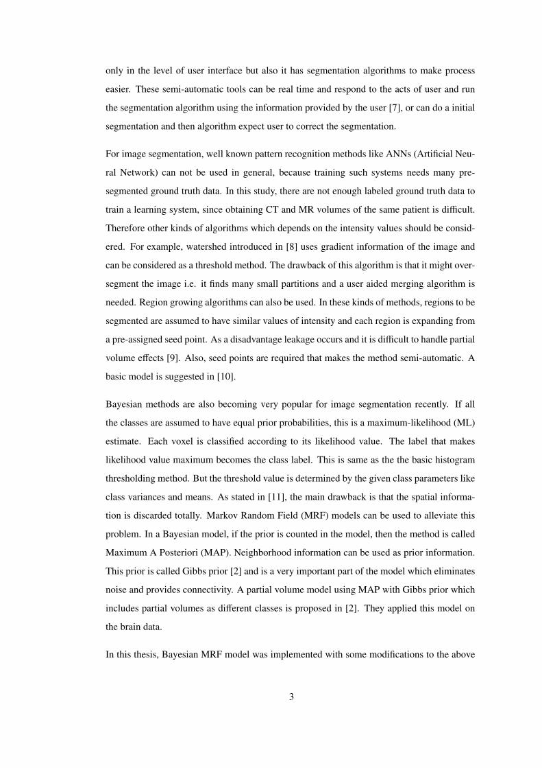
(a) (b)

Figure 2.1: Implicit Surface (ϕ) and its zero level set shown by red contour. (a) Side view (b)Upper view (Projection to the x-y plane)

Here ϕ is the implicit function whose zero level set is a curve defined as C. The implicit

function is defined as a function of C such that ϕ is a signed distance function. Every point

in the grid takes the value of its distance to the curve C. If a point is inside the curve, it

takes a negative value and vice versa. If a point is on the curve (C), then it takes the value

of zero. An example curve C (the red curve) and its distance function ϕ (conical shape in

3D) is illustrated ind Figure 2.1. In the illustration, the curve C is in two dimensions and

the corresponding implicit function is three dimensional. The Level Set method carries the

problem to higher dimension, as depicted in 2.1. Now many different closed curves in 2D

are defined as zero level sets of one implicit function (ϕ) in 3D. As the curves evolve in time

(under the effect of speed function F), splitting and merging of boundaries may happen, with

level set method, these changes are implicitly handled. This very important result is one of

the aspects that makes Level Set method powerful.

Signed distance function is Lipschitz continuous everywhere, except in the center of the curve

(but it does not have a negative affect in practical application). It is differentiable everywhere,

also near the boundary (C). These properties makes signed distance function an appropriate

selection for the partial differential equations.

The level set equation comes with its nice properties, yet the numerical solution should keep

these nice properties. The numerical solution to the level set equation has to be both stable

and convergent. Stability refers to numerical solutions handle numerical errors such that nu-

merical errors are not being accumulated in time. Convergency means that the steady state

solution is reachable in finite time steps. In the next section, a numerically stable and conver-

8

gent Level Set solution will be provided. Instead of Equation 2.1, the convection form of the

Level Set Equation (Equation 2.3) (the motion in externally generated field) will be discussed,

because these two equations can be derived from each other (Appendix B) and the numerical

solution to the motion in externally generated field is more comprehensible.

2.1.1 Motion in an Externally Generated Velocity Field

Assume that there is a boundary defined by zero level set of implicit function (ϕ), ϕ(x) = 0

and a velocity field, V(x) in 3D, x where V = ⟨u, v,w⟩. The simplest method to move all the

points according to this velocity field is solving

dxdt= V(x) (2.2)

for every point x. The front of the curve has to be discretized, but there are infinitely many

points in the front. In every time step, it has to be discretized again to provide a correct numer-

ical solution. In 2D, segments and in 3D, triangles can be used for discretizing [27]. This is

not an issue if the front holds its connectivity. But even under the simplest velocity field large

distortions forms, so front should be regularized and smoothed [26]. The topology changes

are hard to handle. This equation is Lagrangian formulation. This Lagrangian formulation

with regularizing, smoothing and surgical operations are called front tracking methods. Points

for 2D and triangles for 3D has to be used as mentioned in [27]. Deformable Model [25] is

a front tracking method as stated in the beginning part of this chapter. Instead of Lagrangian

formulation the Level Set formulation,

ϕt + V · ∇ϕ = 0, (2.3)

which enjoys the properties of Hamilton-Jacobi Equations is in the scope of this study. In

the Equation ϕt is time derivative of the implicit function and ∇ϕ = ⟨ϕx, ϕy, ϕz⟩. If gradient

operator is written in open form we have

V · ∇ϕ = uϕx + vϕy + wϕz. (2.4)

This type of Level Set equation (Equation 2.3) where there is an external vector field (V)

is also used in combustion reaction model. For combustion reaction ϕ = 0 represents the

surface of reaction of a moving flame front [27]. This equation is sometimes called convection

equation. In this study it is also referred as convection equation. Numerical solution of the

Equation 2.3 will be given in following sections.

9

2.1.1.1 Discretization of Convection Equation and Upwind Differencing Methods

The discretization of the Equation 2.3 in time could be done with forward euler time or back-

ward euler time. Discretization using the latter will be given in 2.1.4. Now Forward Euler

Time is the one to be focused at: At time t we have the values ϕn = ϕ(tn) and at tn+1 = tn + ∆t

we have ϕ(tn+1). Then discretizing in time with forward euler step is

ϕt =ϕn+1 − ϕn

∆t. (2.5)

Write this in Equation 2.3 to obtain,

ϕn+1 − ϕn

∆t+ Vn · ∇ϕn = 0. (2.6)

Spatial derivatives: One can evaluate spatial derivatives using this straightforward approach

used for time derivation, but it does not give a stable solution. More effort is needed, So we

start by writing the Equation 2.3 in expanded form in 3D,

ϕn+1 − ϕn

∆t+ uϕx + vϕy + wϕz = 0. (2.7)

This equation can be discretized in dimension by dimension manner. For the sake of sim-

plicity, the equation is now only for one dimension x and for a specific grid location i and

written,ϕn+1

i − ϕni

∆t+ un

i (ϕx)ni = 0, (2.8)

where ϕni is the spatial derivative of ϕ at the point xi. When ui > 0, the values of ϕ or the

information is moving from left to right. Method of characteristics tells to take the spatial

information from left to calculate which value of ϕ will take place on xi. Then a first order

scheme∂ϕ

∂x=ϕi − ϕi−1

∆x(2.9)

for ui > 0 is written. This is a first order accurate backward difference spatial discretization

operation and symbolized as D−ϕ (where D−ϕ is the backward difference operator). If ui < 0,

the values of ϕ now are moving from right to left and we should take the spatial information

from right of the point xi, then this scheme

∂ϕ

∂x=ϕi+1 − ϕi

∆x(2.10)

10

is used. Similar to the backward difference scheme, this is first order accurate forward dif-

ference and operation is symbolized as D+ϕ (where D+ϕ is the forward difference operator).

Using the spatial information in the direction opposite to the moving direction of the values of

ϕ is called upwinding [27]. Verbally spoken, when u is positive, vector field has a component

heading to right, the value of the implicit function and information moves right. Upwinding

method takes the spatial information from left and vice versa when u is negative.

2.1.1.2 Hamilton-Jacobi Essentially Non-Oscillatory Schemes

The upwinding methods introduced in the previous section can be improved to have better ap-

proximation. In this manner the number of points to calculate the numerical spatial derivative.

A good approximation should be smooth and represent data well. Hamilton-Jacobi Essentially

Non-Oscillatory (HJ ENO) are designed [28], [29] based on these two aspects. These schemes

are 1st, 2nd, 3rd and 5th order. The first three are given in Appendix C. But to summarize the

first one it is the first order upwinding scheme described in Section 2.1.1.1. The second and

third order approximation uses second and third order derivative approximations respectively.

For these higher order terms scheme selects the direction which gives a smaller change in

the function. Taking information from less smooth direction is not desired. With this choice

higher order derivatives do not create oscillations. For every grid point and for every time

step schemes select one of two stencils: right biased or left biased. In HJ Weighted Non-

Oscillatory Scheme (HJ WENO) instead using this selection criteria a weighted interpolation

of these four stencils are used. Weights change according to their smoothness and smoothness

is measured using Equations 2.15,2.16 and 2.17. Following paragraphs gives the procedure

in detail.

For the approximation of ϕ−xithe third order HJ ENO uses subset of the left biased stencil

ϕi−3, ϕi−2, ϕi−1, ϕi, ϕi+1, ϕi+2. As in [30] the subset stencils are ϕi−3, ϕi−2, ϕi−1, ϕi, ϕi−2, ϕi−1, ϕi, ϕi+1

and ϕi−1, ϕi, ϕi+1, ϕi+2 (see Figure 2.2).

Let’s define v1 = D−ϕi−2, v2 = D−ϕi−1, v3 = D−ϕi, v4 = D−ϕi+1 and v5 = D−ϕi+2 as defined in

[27]. Where D’s are differencing operator as defined in Section 2.1.1.1. Then three possible

ϕ−xiare

11

Figure 2.2: Three subsets of the stencil: (a) Left biased stencil to calculate ϕ−xi(b) Right biased

stencil to calculate ϕ+xi[30].

ϕ1x =

v1

3− 7v2

6+

11v3

6(2.11)

ϕ2x = −

v2

6− 5v3

6+

v4

3(2.12)

and

ϕ3x = −

v3

3+

5v4

6− v5

6(2.13)

Proceeding in the lines of [27] it is seen that in [28] it was proposed to use a convex combina-

tion of three possible 3rd order difference schemes to obtain a smooth interpolation of the data

and they called the method WENO (Weighted ENO). The weights are chosen in such a way

that finite difference calculated next to a discontinuity is given the value of zero. In smooth

regions, all three approximations equally effects the interpolation. After, in [29] Jiang et. al.

calculated optimal weights. They obtained 5th order accuracy in smooth regions. Later [30]

modified the WENO and adapted in to the HJ framework. Now in the following paragraphs

the HJ WENO will be explained. The weighted polynomial is given

ϕx = ω1ϕ1x + ω2ϕ

2 + ω3ϕ3 (2.14)

where 0 < ωk 6 1 and ω1 + ω2 + ω3 = 1. This equation is convex combination of ω1,ω1 and

ω3 which were given in equations (2.11), (2.12) and 2.13. The optimal weights for smooth

regions are ω = 0.1, ω = 0.6 and ω = 0.3. But in non smooth regions only one of the stencils

is used to provide backward difference, ωk = 1 and the other weights are 0. In [30] in order

to define weights they have used smoothness metrics of stencils such as

12

S 1 =1312

(ν1 − 2ν2 + ν3)2 +14

(ν1 − 4ν2 + 3ν3)2, (2.15)

S 2 =1312

(ν2 − 2ν3 + ν4)2 +14

(ν2 − ν2)2 (2.16)

and

S 3 =1312

(ν3 − 2ν4 + ν5)2 +14

(3ν−4ν3 + ν5)2. (2.17)

Then new variables which depend on these smoothness measures are given,

α1 =0.1

S 1 + ϵ(2.18)

α2 =0.6

S 2 + ϵ, (2.19)

and

α3 =0.3

S 3 + ϵ. (2.20)

If a region is smooth, corresponding α value becomes large. ϵ is scale factor suggested in [31]

and is defines as,

ϵ = 10−6ν21, ν22, ν23, ν24, ν25 + 10−6 (2.21)

.

In smooth regions, S k’s goes to 0 and when they are negligibly small comparing to ϵ then

coefficients become. α1 ≈ 0.1ϵ2,α2 ≈ 0.6ϵ2 and α3 ≈ 0.3ϵ2. The ak’s are normalized to

obtain weights

ω1 =α1

α1 + α2 + α3, (2.22)

ω2 =α2

α1 + α2 + α3(2.23)

and

ω3 =α3

α1 + α2 + α3. (2.24)

and if we continue the calculation in a smooth region,ω1 =0.1ϵ2

0.1ϵ2+0.6ϵ2+0.3ϵ2 = 0.1 and similarly

ω2 = 0.6, ω3 = 0.1. For example, if one of the stencils are discontinuous , related S k will be

large and related coefficient ω will be a small value and will have a little contribution to the

final approximation. If two of them have discontinuities then related coefficient will be small

13

and the other will dominate. The last condition where each three stencils have discontinuities

is a difficult case for HJ ENO and is very rare and the problem is alleviated in time.

Here only approximation of ϕ−x is given, similar procedure should be followed for ϕ+x in right

biased stencil (Figure 2.2).

2.1.1.3 Convergency and Stability

The Lax-Richtmayer equivalence theorem says that a finite difference approximation to a

linear partial differentiation is convergent (the solution is correct when ∆t → 0 and ∆x → 0)

if the solution is consistent and stable. The discretizing with upwinding and forward euler is

consistent because the approximation error is 0 when ∆t → 0 and ∆x→ 0.

Stability means that small roundoff errors in the numerical scheme does not grow in time.

Stability can be obtained by Courant-Freidreichs-Lewy (CFL) condition. This condition says

numerical waves should propagate faster than the physical vector field. The CFL time step

restriction is,

∆t <∆x

max|u| . (2.25)

Here max|u| is the maximum speed of the numerical wave. And to determine time step (∆t)

which makes the solution stable, a parameter is introduced such as,

∆tmax|u|∆x

= α (2.26)

and 0 < α < 1. In 3D CFL restriction can be written as

∆tmax |u|∆x+|v|∆y+|w|∆z = α (2.27)

or,

∆tmax|V |

min∆x,∆y,∆z == α. (2.28)

|V | is magnitude of the velocity field such as

|V | =√

u2 + v2 + w2. (2.29)

In our problem ∆x = ∆y = ∆z = 1 and does never change so to provide stability in every

iteration time step has to be calculated according to Equation 2.27 or alternatively Equation

2.28.

14

2.1.2 Hamilton-Jacobi Equations

In this section, a general solution method of Hamilton-Jacobi equations of the form

ϕt + H(∇ϕ) = 0 (2.30)

will be discussed. Convection Equation 2.3 and level set Equation 2.1 are Hamilton-Jacobi

equations. This generalization is last step to give a numerical solution to the standard level

set solution. In following paragraphs the methods applied to solve convection equation is

generalized by examining Hamilton-Jacobi equation, The HJ equation in three dimensions is

ϕt + H(ϕx, ϕy, ϕz) = 0. (2.31)

H(ϕx, ϕy, ϕz) = V · ∇ϕ. The numerical discretization in time using Forward Euler time gives

ϕn+1 − ϕn

∆t+ H(ϕ−x , ϕ

+x ; ϕ−y , ϕ

+y ; ϕ−z , ϕ

+z ) (2.32)

where H(ϕ−x , ϕ+x , ϕ

−y , ϕ

+y , ϕ

−z , ϕ

+z ) is the discrete Hamiltonian. If |H1| = ∂H

∂ϕx,|H2| = ∂H

∂ϕyand

|H3| = ∂H∂ϕzis define the CFL time step restriction as stated in Section 2.1.1.3 is

∆tmax|H1|∆x+|H2|∆y+|H3|∆z

< 1 (2.33)

The Hamiltonian for Convection Equation (Equation 2.3) is H(ϕx, ϕy, ϕz) = uϕx + vϕy + wϕy.

Note that numerical Hamiltonian H is the function of backward (ϕ−x , ϕ−y , ϕ

−z ) and forward

(ϕ+x , ϕ+y , ϕ

+z ) differences. These difference can be calculated with HJ ENO or HJ WENO

schemes. For every dimension there are two options: ϕ+x ϕ−x . To obtain the numerical cor-

rect solution the right one has to be chose.The following numerical method is to tell which

one is a better choice. This method is called Godunov’s scheme, in two dimensions it is:

H = extxextyH(ϕx, ϕy) (2.34)

Here extx is defined as: if ϕ−x > ϕ+x then H takes the minimum value in the interval where

Iϕx ∈ ϕ−x , ϕ+x and if ϕ−x < ϕ+x H takes the maximum value in the interval. For y and z same

procedure can be followed. In applications the order of extx,exty and extz effects the solution,

but in our problem this will not change the solution since extxextyH = extxextyH. There are

six possibilities for 3D but they are all equal again for our problem.

Let’s get back to the convection (Equation 2.3) to see its numerical solution by Godunov’s

scheme. Hamiltonian H is separable: extxextyH(ϕx, ϕy) = extx(uϕx) + exty(vϕy). In the case,

15

where ϕ−x < ϕ+x ,the minimum value of uϕx should be chosen according to Godunov’s Scheme

and this choice depends on the sign of u. If u is positive (u > 0), uϕ−x is selected and if u is

negative (u < 0), uϕ+x is selected. Similarly when ϕ−x > ϕ+x the maximum is picked by the

scheme: The scheme chooses maximum possible value of uϕ−x and it depends on the sign of

u. If it is negative (u < 0), the scheme chooses uϕ+x ; else the scheme chooses uϕ−x . When

u = 0 the choice is trivial. To summarize these operations , scheme says: If u < 0 use ϕ+x ;

if u > 0 ,use ϕ−x and if u = 0, the result is regardless of the choice. In conclusion, Godunov

scheme for convection equation is simple upwinding scheme described in Section (2.1.1.1)

for the Equation 2.3.

Godunov scheme is not only the scheme to solve Hamilton-Jacobi equations. Schemes like

Roe-Fix Scheme,and Lax-Friedrichs schemes can be used also. In this study Godunov Scheme

is used, because it is easy to implement and gives sufficiently good results.

2.1.3 Motion in Normal Direction

The equation of motion in normal direction is the general Level Set Equation 2.1. Let’s rewrite

it:

ϕt + F|∇ϕ| = 0. (2.35)

As stated earlier, it is a Hamilton-Jacobi equation and the numerical methods are mentioned

in Section 2.1.1. In Hamilton-Jacobi model solutions, we need H1, H2 and H3 which are the

partial derivatives of the Hamiltonian (H) with respect to ϕx, ϕy, and ϕz respectively in 3D.

Here in Equation 2.35, H = F|∇ϕ|. Note that, |∇ϕ| =√ϕ2

x + ϕ2y + ϕ

2z then

H1 = F∂H∂ϕx= F

2ϕx

2|∇ϕ| = Fϕx

|∇ϕ| . (2.36)

Similarly,

H2 = Fϕy

|∇ϕ| (2.37)

H3 = Fϕz

|∇ϕ| (2.38)

can be written following the steps to find H1. If we write the equation convection form,

ϕt +

(Fϕx

|∇ϕ| + Fϕy

|∇ϕ| + Fϕz

|∇ϕ|

)· ∇ϕ = 0 (2.39)

16

it is easier to compare Equation 2.3 with Equation 2.35. Recall that in motion by externally

generated field (Equation 2.3) V = ⟨u, v,w⟩ and here we have ⟨u, v,w⟩ = ⟨H1,H2,H3⟩. The

connection between convection Equation 2.3 and 2.35 is clear now. All methods prescribed

before are all applicable.

The time step restriction can be found using Equation 2.33 by plugging the values of H1,H2

and H3.

For spatial discretization of this type of equation as stated earlier Godunov scheme is used. In

Table 2.1 the method is summarized. Where ϕ−x < 0 and ϕ+x > 0 (V-shaped expansion region)

two partial derivatives have different signs. In expansion characteristics of the equation data is

in both direction and outwards. Godunov scheme minimizes H (since ϕ+x > ϕ−x ) by choosing

the ϕx = 0. In an an expansion region function should be locally smooth [27]. Godunov

provides this without adding artificial dissipation (second order partial derivatives). Godunov

avoids the error introduced by artificial dissipation. At grid points where ϕ−x > 0 and ϕ+x < 0,

the information is coming from both sides causing shock. Godunov maximizes H (since

ϕ−x > ϕ+x )by choosing the fastest of derivatives reaching that point. Then maximization ends

up with choosing the larger of ϕx in magnitude. Again problem is circumvented without

artificial dissipation. The other cases are simple upwinding discussed before.

Table 2.1: The spatial derivative choices of Godunov Scheme, ϕ is the level set function andsubscripts x and y are to represent partial derivatives. F is a scalar on the coordinates (x, y)

ϕ−, ϕ+ > 0 ϕ−, ϕ+ > 0ϕ− < ϕ+ ϕ− > ϕ+ ϕ− < ϕ+ ϕ− > ϕ+ ϕ+ > 0, ϕ− < 0 ϕ+ < 0, ϕ− > 0

F > 0 ϕ−x ϕ−x ϕ+x ϕ+x ϕx = 0 max|ϕ−x |, |ϕ+x |F < 0 ϕ+x ϕ+x ϕ−x ϕ−x ϕx = 0 min|ϕ−x |, |ϕ+x |

2.1.4 Curvature Evolution

Curvature evolution is an important aspect in curve evolution methods. In our solution

method, curvature evolution is important. In curvature evolution, curve moves under effect of

its curvature. It is different from convection since movement depends on the internal proper-

ties of the curve. The points with higher curvature will move faster. So the curve becomes

much smoother until it becomes a circle. Finally, it collapses i.e. shrinks to a point.

17

Here in this section, numerical methods will be given to solve the equation. Only shrink-

ing evolution is discussed and is used in algorithms since curvature growing is an ill-posed

problem and error increases in time leading wrong solutions.

Recall the Equation 2.1,

ϕt + F|∇ϕ| = 0. (2.40)

Now set F = −bκ where b is constant and greater than zero and κ is the mean curvature of the

implicit function (ϕ). Definition and derivation of mean curvature for 2D and 3D is given in

Appendix D.

When F plugged into the Equation 2.1

ϕt = bκ|∇ϕ|. (2.41)

is obtained. In the curve evolution on the coordinates where the shape is convex, mean cur-

vature will be positive and the points will propagate inwards and in concave regions mean

curvature will be negative resulting in the motion outwards. In Figure 2.3 the signs of curva-

tures are illustrated and in Figure 2.4 an example of mean curvature evolution is illustrated.

In the figure it is easy to see the direction of motion is outwards in concave and inwards in

convex regions. Also note that the amount of propagation is larger in the regions where the

curvature is large in magnitude. Hence the shape shrinks and before collapsing it takes a

round form (which is a circle in 2D and sphere in 3D).

Forward time step is an appropriate solution, but since the right side depends on curvature

(so on second derivatives of the implicit function ϕ), the equation is parabolic and not hyper-

bolic. Therefore upwinding methods used for advection Equation 2.3 cannot be used. The

information does not come from only one direction, rather is coming from both directions.

As a result, central difference scheme for spatial derivative is appropriate. Remembering that

central difference approximation is:

ϕx =ϕi+1 − ϕi−1

2∆x(2.42)

Then CFL time restriction is

∆tmax

2b(∆x)2 +

2b(∆y)2 +

2b(∆z)2

< 1. (2.43)

18

Figure 2.3: Curvature directions on the boundary [27].

It restricts the time step a lot because denominator is now squared. Making time step smaller

loads a high burden to the numerical solution. It decreases the time step (δt) more and in-

creases the number of steps until convergence. Another numerical method which does not

bring any restriction to time step selection is Backward Euler Method. The mathematical

details as in [20] is given in Appendix E.

2.2 Geometric Integral Measures

Until here in this Chapter, numerical methods to solve level set equations were given. But

nothing about the scalar field F in Equation 2.1 was discussed. F determines the motion of

the curve. In this section mathematical background of deriving scalar function F from energy

functionals E(C) that depends on the evolving curve C is given. These energy functionals

are integrals over a region (enclosed or disclosed by C) or closed contour integrals on the

boundary (C). The level set solution will find the curve C which minimizes the integral. The

general variational procedure to obtain speed terms (F) minimizing an energy integral can be

summarized as this:

(i) The energy functional E(C) is defined, (ii) The first variation δEδC is calculated. The result is

19

Figure 2.4: Curvature motion of a star shaped curve [27].

the curve evolution equation Ct = − δEδC where Ct is velocity of the curve. (iii) Speed function

F is related a sCt = n. Finally we plug speed function F into the level set Equation 2.1.

In the next two Sections (2.2.1 and 2.2.2), this procedure will be applied and the segmentation

model is described.

2.2.1 Geodesic Active Contours, Surfaces

This term was first introduced in [18] and explained using variational framework. In this

section, we will follow the derivation which was given in the study. First, let’s examine a

general contour integral measure in 2D. Where g is a scalar function.

E(C) =∮

Cg(C(s)) ds. (2.44)

20

After taking first variation and arrange it in the level set form (see Appendix E) the equation

ϕt =(κg − ⟨∇g.∇ϕ|∇ϕ| ⟩)|∇ϕ| (2.45a)

ϕt =κg|∇ϕ| − ⟨∇g,∇ϕ⟩|∇ϕ|. (2.45b)

is obtained. Notice that if g is chosen to be 1 everywhere, then we have

ϕt = bκ|∇ϕ|. (2.46)

It is the Equation 2.41, motion of a curve shrinking under its own curvature as given in previ-

ous Section 2.1.4. In our segmentation model we need smoothing but also we need to preserve

sharp structures like thin muscles. The Edge indicator is a stopping function:

g(I) =1

1 + |∇Gσ ∗ I|2 (2.47)

where G is gaussian with variance σ. The denominator is smoothed image gradient. for 2D

it is G2x +G2

y and in 3D it is G2z +G2

y +G2z . The Gx, Gy and Gz are smoothed image gradients

in x,y,z directions respectively. g becomes small when the gradient is large as illustrated in

Figure 2.5. It is positive everywhere. It was previously used in the model called geometric

active contour model [16]:

ϕt = g(I)div(∇ϕ|∇ϕ|

)+ cg(I)|∇ϕ|. (2.48)

This model is similar to Geodesic Active Contours (GAC) model introduced in Equation

2.45b but second term is different. Here g is used as balloon force (or weighted area term).

The curve evolution stops where the gradient is large and g is 0. But only in the perfect

edges g takes the value 0. In real images especially in medical data because of noise there are

many zeros that are not edges. In these regions this model stops. Also one drawback is that

this term is positive everywhere, meaning that curves evolves in one direction so the result

depends more on the initialization.

In the new GAC model, instead of second term, there exists ⟨∇g,∇ϕ⟩ which drags level set to

the valleys of function g (Figure 2.5). In addition, the balloon force (as in earlier proposed

model i.e. Geometric model [18]) can be added to the model to make iterations converge

faster. Then the whole model is achieved:

Ct = (−cg − κg + ⟨∇g.n⟩) n (2.49)

21

Figure 2.5: 1D illustration of the GAC model, (a) I vs x, An edge in an image(I) (b) ∇Gσ∗ I vsx, smoothed version of (a). (c) Edge indicator function g and directions of the curve throughthe valleys [18].

where c is a scalar. Now the model is named Geodesic rather than Geometric. In this study,

balloon force term is dropped since we need accuracy rather than speed.

2.2.2 Minimum Variance

It is an energy term based on the Mumford-Shah model [14]. Chan and Vese approximated

and solved this functional efficiently by using Level Set methods in [15]. The derivations

again will be given for 2D (contours) for the sake of simplicity. The 3D extension is straight-

22

forward and trivial. Minimal variance energy functional is:

E =12

∫ ∫ΩC

(I − c1)2dxdy +∫ ∫

Ω/ΩC

(I − c2)2dxdy (2.50)

Minimizing this functional means to find the curve C separating space into two smooth regions

(i.e. variances of inner and outer regions are small). This is why this term is called minimum

variance term. The corresponding level set equation is:

ϕt + (c1 − c2)(I − c1 + c2

2

)|∇ϕ| = 0. (2.51)

where c1 and c2 are average values (see Appendix F for the full derivation) of inner and outer

regions. In the evolution process, boundary avoids from the background mean c2 and trying to

be close to the mean c1. Every step c1 and c2 are supposed to become closer to the real mean

of the regions that we are trying to segment. As can be seen easily, Equation F.17 becomes

zero at places where I = c1+c22 , negative if I < c1+c2

2 and positive when I > c1+c22 . This means

the curve will shrink in the background region where I > c1+c22 , will expand in the desired

region where I < c1+c22 and will stop in the boundary where I = c1+c2

2 .

In [15] the reason why they call the model active contours without edges is that curve does not

need the edge information as geodesic active contour do so. As a result, this terms works well

in noisy data case because, if the noise has zero mean, it does not effect the mean intensity

values of the classes.

2.3 Level Set Segmentation Model

Here in this section, the Level Set segmentation model used to segment muscles is described.

The Level Set segmentation model used in this study is a binary segmentation model i.e. it

separates foreground from background. The objective is to segment face muscles but in human

head data there are several tissue types. These are mainly skin, veins, glands, muscles, fat,

bone (skull and teeth), marrow and air. In CT and MRI, glands, muscles and veins have similar

intensity values so in this study they are considered as same class and called Muscle class. The

marrow is inside the bone and resides in the cavities of the bone, so marrow, teeth and skull are

considered as same class and named Bone class. The skin tissue has intensity values similar

23

to Muscle class but treated as a different class. It is not possible to segment these classes

using one binary segmentation step. It is possible to do hierarchical level set segmentation

to segment more than two classes [20] but here, in this thesis other classes are segmented

using simpler image processing techniques. There are two main reasons: Firstly Level Set

method is a computationally expensive method and secondly, (mimic muscle segmentation

is the main focus of this study) there is no need for high accuracy segmentation for classes

other than Muscle. These simple image processing methods will be called preprocess and

postprocess steps of the model. Level Set segmentation process is compromised of three

parts: (i) preprocess, (ii) solving level set equation (main part) and (iii) finally postprocess.

The complete model is provided in Figure 2.6.

The objective of the Preprocess step is to remove Air and Bone classes from images and then

to provide initial segmentations using K-means method (Section 2.3.1). Main Part does the

actual segmentation using Level Set segmentation methodology (Section 2.3.2). Post Process

has two parts: The first part is optional which will be explained in Section 2.3.3.

2.3.1 Preprocess

Preprocess has two main goals the first is to eliminate tissues that is not in the focus of this

study. These classes are Bone and Air and these two classes have the respectively highest and

lowest mean intensity value in CT image. So applying two thresholds (172 HU for upper and

-609 HU for lower threshold) on CT data Air and Bone can easily be removed and is used as

a binary mask: In the regions of interest (Muscle and Fat) Mask takes the value of 1 otherwise

0. In the Main segmentation part only the information where mask is nonzero is used. The

marrow tissue resembles muscles so in this thresholding process the marrow tissues is not

removed. But it is known that marrow is inside bone. Therefore if the bone is filled using

binary flood fill operation the marrow is also removed and this completes the mask and first

part of Preprocess.

The second part’s aim is to provide a initial segmentation to help level set algorithm con-

verge faster and prevents it from getting stuck in local minima. The K-means algorithm is

used for this purpose. The K-means algorithm is a basic iterative clustering algorithm and

it finds predefined number of classes and classifies voxels based on their distances to cluster

means. In this part, the image is separated into two regions foreground (initial Muscle class)

24

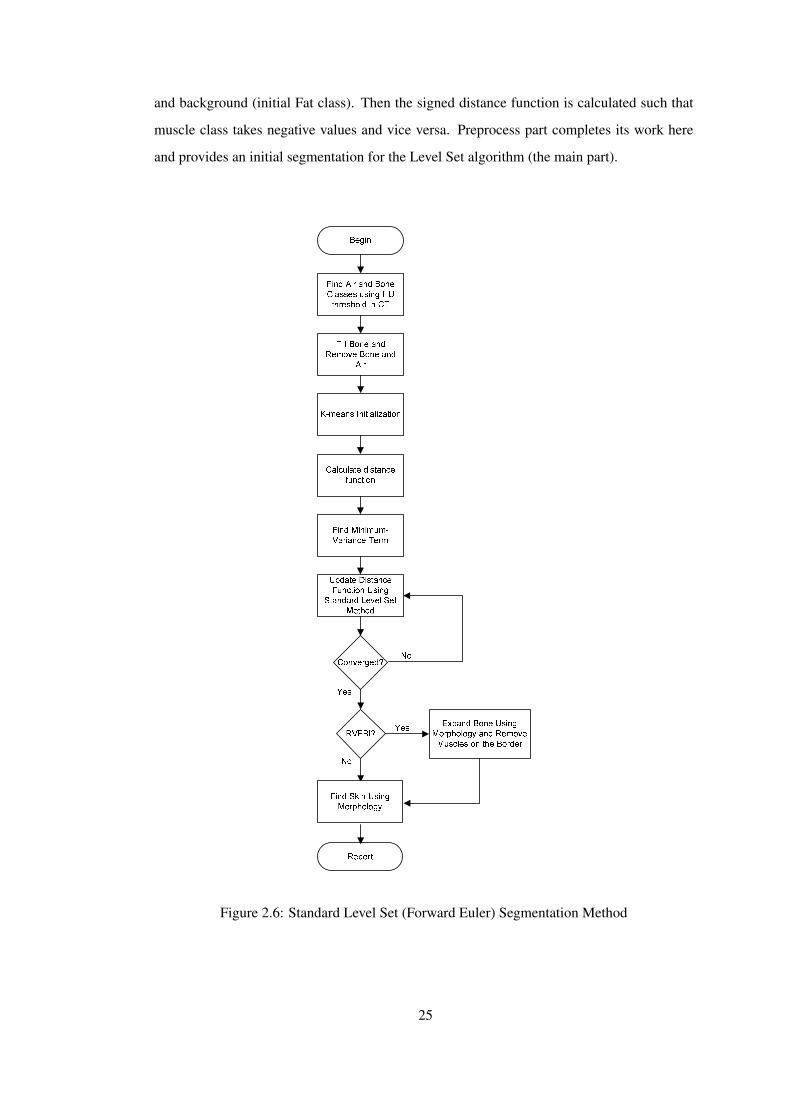
and background (initial Fat class). Then the signed distance function is calculated such that

muscle class takes negative values and vice versa. Preprocess part completes its work here

and provides an initial segmentation for the Level Set algorithm (the main part).

Figure 2.6: Standard Level Set (Forward Euler) Segmentation Method

25

2.3.2 Main Part

In Figure 2.6 blocks in between ‘K-means Initialization’ and ‘RVBFI’ forms main part of

the standard Level Set model. The main part is the Level Set solution of the segmentation

problem. It uses numerical methods and theory described before in previous sections. These

methods are combined accordingly to obtain the main part. If geodesic term and minimum

variance terms are weighted with scalars (α, β) and combined in one level set equation one

obtains:

ϕt =

α (κg − ⟨∇g.n⟩) + β

[(c2 − c1)(I − c1 + c2

2)]|∇ϕ|. (2.52)

This is the model for one type of modality (either MR or CT ). It is possible to obtain better

results if MRI and CT modality images are unified. In this case mean intensities (c1 and c2)

and image intensity value I of each modality constitutes the Minimum Variance term:

FMV = γ(cMR2 − cMR

1 )IMR −

cMR1 + cMR

2

2

+ (1 − γ) (cCT2 − cCT

1 )ICT −

cCT1 + cCT

2

2

(2.53)

where γ is the weighting factor and γ ∈ [0, 1] which determines the effect of the modality to

the equation. γ is the third parameter with α and β (all are positive scalars).

Similarly geodesic term is also modified for unified data. The stopping function g was modi-

fied to metric tensor G as in [32][33],

G =M∑

b=1

I2

x IxIy IxIz

IyIx I2y IyIz

IzIx IzIy I2z

(2.54)

where the elements of the matrix are partial derivatives of images, b is the number of bands

(in our case M = 2: MRI and CT data). For an edge, the differences between maximum and

minimum eigenvalue is large.Therefore edge indicator function for unified data was chosen

as:

g(I) =1

1 + (λ+ − λ−)(2.55)

26

Where (λ+) is the maximum eigenvalue and (λ−) is the minimum eigenvalue.

In the model, first term (the geodesic part) does the smoothing (diffusion) using edge infor-

mation and second term (minimum variance term) is creates the discontinuity in the level set

function and separates space in two regions. The model seeks for regions with uniform inten-

sity inside and outside with smooth boundaries in between. The balance of two terms create

the regions. Less smoothing may result in noisy boundaries while much smoothing may result

in over smoothed boundaries or may cause the level set completely collapse to a point.

In Equation 2.52: The geodesic part has a curvature term that is parabolic and remaining parts

are hyperbolic. Minimum variance term has only one solution option that is the Forward Euler

solution. But for the parabolic part there are two options, Explicit Solution (Forward Euler

Time) and Implicit Solution (Backward Euler Time) which were discussed in Section 2.1.4.

Explicit Model: For explicit solution, as in Section 2.1.3 hyperbolic terms H1, H2 and H3

are defined as H1 = FHϕx|ϕ| , H2 = FH

ϕy|ϕ| and H3 = FH

ϕz|ϕ| where in our model FH =

α⟨∇g.n⟩ + β[(c1 − c2)(I − c1+c2

2 )]

is the hyperbolic part and FP = κg. So the CFL condi-

tion for hyperbolic terms (as described in Equation 2.33) and parabolic terms (Equation 2.43)

are combined to write

∆t max|H1|∆x+|H2|∆y+|H3|∆z+

2g(∆x)2 +

2g(∆y)2 +

2g(∆z)2

< 1. (2.56)

CFL condition above gives the time step. So for one dimension update equation is

ϕn+1 = ϕn + ∆t(F|∇ϕnx|). (2.57)

Spatial derivatives are found using Hamilton-Jacobi Essentially Non Oscillatory schemes in

desired accuracy (one up to five order).

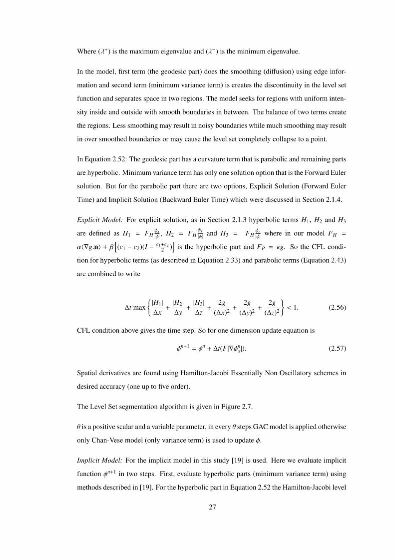
The Level Set segmentation algorithm is given in Figure 2.7.

θ is a positive scalar and a variable parameter, in every θ steps GAC model is applied otherwise

only Chan-Vese model (only variance term) is used to update ϕ.

Implicit Model: For the implicit model in this study [19] is used. Here we evaluate implicit

function ϕn+1 in two steps. First, evaluate hyperbolic parts (minimum variance term) using

methods described in [19]. For the hyperbolic part in Equation 2.52 the Hamilton-Jacobi level

27

i← 1Initialize ϕ to a signed distance function.while |ϕn − ϕn+1| > ϵ do

Compute means c1 and c2 using Equations F.18c and F.18dif mod (i, θ) == 0 then

Find curvature κ of ϕ and calculate κg.Find normals n of ϕ and calculate ⟨∇g.n⟩

end ifCalculate H1, H2 and H3 using Godunov SchemeCalculate ∆t using Equation 2.56ϕ← ϕn+1 (Equation 2.57), i← i + 1

end while

Figure 2.7: Forward Euler Time Level Set Algorithm

set methods are used. Alternatively, the equation could be simplified replacing |ϕ| = 1 since

ϕ is signed distance it is considered a good approximation and time step is predetermined by

the user as a parameter. Then hyperbolic part reduces to:

ϕint = ϕk + ∆kβ[(c1 − c2)(I − c1 + c2

2)]. (2.58)

where k is time, ∆k is time step and ϕint is the intermediate result that will be used in next

equation:

ϕk+1 = (I − ∆kA1)−1(I − ∆kA2)−1(I − ∆kA3)−1(ϕint). (2.59)

Here a problem arises: If ϕint is calculated using Hamilton-Jacobi methods, the time step will

be calculated using CFL restriction. But for second part time step ∆k is predetermined by

user. So the equation is not solved in same time step (unlike the Explicit solution described in

first part of this section). These solutions are different steps and can not be considered as one

level-set solution [34]. For the intermediate part if simplified version (Equation 2.58) is used

now same time step is used. This may cause algorithm produces instable results if enough

diffusion is not introduced in mean curvature step [34]. Despite these theoretical drawbacks

practically this method is still useful and converges faster, since it allows larger time steps

(Numerical solution is unconditionally stable according to [19]).

28

The segmentation procedure is similar to one given in [34] for implicit model:

The segmentation algorithm for implicit model is given in Figure 2.8. For more details about

updating step see Appendix G.

i← 1Initialize ϕ to a signed distance function.while |ϕk − ϕk+1| > ϵ do

Compute means c1 and c2 using Equations F.18c and F.18d;ϕ← ϕint ,Equation 2.58if mod (i, θ) == 0 then

Re-initialize ϕ to signed distance functionϕ← ϕk+1 ,Equation 2.59

end ifi← i + 1

end while

Figure 2.8: Backward Euler Time Level Set Algorithm

θ is a positive scalar and a variable parameter, in every θ steps GAC model is applied otherwise

only Chan-Vese model (only variance term) is used to update ϕ.

The main segmentation part of the Level Set model has three versions:

• Standard-p,

• Standard-a,

• Adaptive,

where first one is standard model with predefined means, second one is the standard model

with automatically calculated class means and third one is thickness adaptive model with

predefined class means. In standard-p, means of Muscle and Fat classes are predefined and

assumed to be same everywhere through out the volume. These mean intensity values for

MR data (which are in [0 255] interval) are listed as: Muscle: 59 and Fat: 148; for CT data

Muscle: 40 and Fat:-106 in Hounsfield Units (HU) scale. However, in standard-a, means of

these classes are calculated in every step as described in Figure 2.7 and Figure 2.8. Adaptive

also uses predefined mean values and is the subject of the next section.

All methods for main part is run for three dimension and two dimensions. Three dimensional

29

versions of these method are tagged with ‘3D’ and two dimensional ones are tagged as ‘2D’

in Chapter 4. In ‘2D’ methods, Level Set equation is solved for each slice of the volume using

only intra-slice information.

2.3.2.1 Adaptive Level Set Segmentation Model

Because of the partial volume problem thin muscles in the image have mean intensity close

to the that of fat class. Henceforth the algorithm decides them as Fat class. The solution

proposed in this study is to detect thin structures in every step and treat them differently. The

segmentation method is described in Figure 2.9.

In every step, (after k-means initialization), algorithm finds thin structures using morpholog-

ical opening. The voxels vanished during morphological opening operations are labeled as

‘Thin’. Other voxels are labeled ‘Non-Thin’. ‘Non-Thin’ regions are expanded using dilation

operation. These voxels also labeled as ‘Non-Thin’. ‘Thin’ labeled muscle and fat classes are

classified again using simple thresholding. These thresholds for ‘Thin’ structures are manu-

ally selected values. For CT data voxels with intensity values greater than -57.5 is classified as

Muscle. For MR data, voxels which have intensity values in between 60 and 110 are classified

as Muscle. This new initial segmentation for ‘Thin’ labeled voxels is to improve segmentation

performance.

Afterwards, algorithm calculates minimum variance terms for two labels (‘Thin’ and ‘Non-

Thin’) separately. For thin regions algorithm uses a predefined mean intensity value (MR:

Muscle: 95, Fat: 137 (in grayscale unit); CT, Muscle: 7 HU, Fat: -106 HU). This is similarly

expected to increase the accuracy in thin regions. The results are provided in Results Chapter

4.

2.3.3 Postprocess

Postprocess step has two parts. The first one is an optional step. The partial volume voxels

on the boundary of fat and bone could have close intensity values similar to the Muscle class.

These voxels are found in one voxel thickness interface between fat and bone. This problem

arises both in MR and CT images since in both case muscle intensity value is between fat and

30

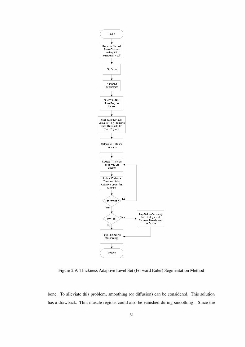
Figure 2.9: Thickness Adaptive Level Set (Forward Euler) Segmentation Method

bone. To alleviate this problem, smoothing (or diffusion) can be considered. This solution

has a drawback: Thin muscle regions could also be vanished during smoothing . Since the

31

position of these problematic voxels are well known on air-bone borders, expanding bone

mask one voxel (using morphological dilate) is an alternate solution. This process will be

called Removing Voxels on the Fat Bone Interface (RVFBI).

The second part of the Postprocess is to find Skin region. The skin is around 3-4 mms thick-

ness for human which corresponds to approximately 4-5 voxels. Using this information, Skin

is found using morphological operations. Erode function is a proper selection after image is

binarized. Firstly, Air region is found using a proper threshold on CT image and then the

remaining part is masked. However sinuses are filled with air and for that reason, if the image

is eroded the structures that are not skin are also removed. To circumvent this problem, the

mask is filled again using flood fill operation slice by slice manner and eroded to set the skin

removed.

In this thesis, there are three types of main parts (‘Standard-p’, ‘Standard-a’ and ‘Adaptive’).

All these were solved in ‘3D’ and ‘2D’ and applied on three data cases (MR only, CT only

and MR&CT unified), with RVFBI and without RVFBI options. In total there are 36 Level

Set methods tested and compared on 16 ROI’s.

2.4 A Bayesian Markov Random Field Segmentation Using a Partial Volume

Model

Our Bayesian Markov Random Field (Bayesian MRF) segmentation model is an extension of

the model described in [2]. They proposed a method for brain segmentation and we applied

the method in [1] and [35] to segment non-brain parts of the head i.e. muscle, fat, bone tissues

and air (both sinus and outside the head). The reason why we chose this method in [1][35]

was that this method handles the partial volume classes. Partial Volume voxels are formed on

the border of tissues during data acquisition and can be seen as a smooth transition in tissue

neighborhoods in the MRI or CT data. Shattuck et. al.[2] classifies these partial volumes as

different classes. Which gives a better classification performance. Below, the segmentation

method of [2][1][35] is summarized and our extensions (adaptive segmentation) are explained.

Segmentation model is Maximum Aposteriori Probability (MAP) classifier based on Bayes

Rule with Markov Random Field. The purpose is to find best label set Λ for the measurement

set (image) X. MAP classifier is [2]:

32

p(Λ|X) =p(X|Λ)p(Λ)

p(X). (2.60)

The likelihood term (p(X|Λ)) is defined based on the assumption that voxels are independently

distributed:

p(X|Λ) =∏k∈Ω

p(xk|λk). (2.61)

Where Ω is the voxel set, xk is intensity values and λk is the label of each voxel. In [2] the

likelihood term is defined for pure classes and partial volume classes. Pure classes are classes

that contains only one class information. The pure classes in our Bayesian model are Bone,

Muscle, Fat and Air. The partial volume classes (mixed classes) are the Fat-Muscle, Bone-

Air, Fat-Bone, Muscle-Air, Muscle-Bone and Air-Bone. The likelihood term for pure class

is:

p(xk|γ) =1

2π√σ

e−12

(x−µ)2σ2 (2.62)

Here, σ is standard deviation and µ is the mean of the gaussian distribution of the class which

has the label γ. The likelihood for mixed classes is:

p(xk|γ) =1

2π√σ1

∫ 1

0e− 1

2(α(x−µ1)−(1−α)(x−µ2))2

σ12 dα. (2.63)

In Bayesian model, prior information is Gibbs prior (i.e. Markov Random Field - MRF) and

calculated using potts model:

p(Λ) =1Z

exp

−η∑k

∑j∈Nk

δ(λk, λ j)

. (2.64)

where δ is a simple comparison function, which is equal to -2 when labels λk and λ j are

equal, -1 when two labels have one common class and 1 otherwise, and η is an uniform,

scalar weighting parameter. This prior probability is to hold connectivity in the segmented

image.

The segmentation is obtained by finding the label set Λ maximizing MAP:

Λ∗ = arg max(p(Λ|X)) (2.65)

This problem is equal to:

Λ∗ =arg max(log(p(Λ|X))) (2.66)

=arg max

log(p(X|Λ)) − η∑

k

∑j∈Nk

δ(λk, λ j)

33

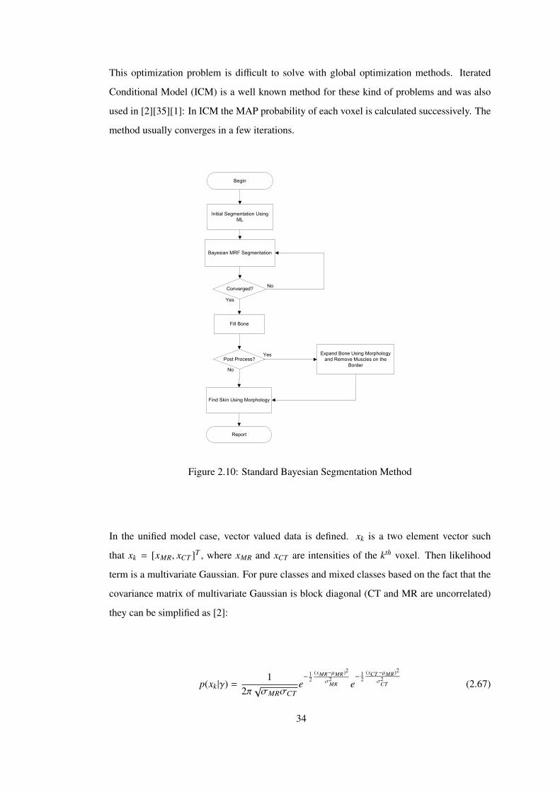
This optimization problem is difficult to solve with global optimization methods. Iterated

Conditional Model (ICM) is a well known method for these kind of problems and was also

used in [2][35][1]: In ICM the MAP probability of each voxel is calculated successively. The

method usually converges in a few iterations.

Begin

Yes

Yes Expand Bone Using Morphology

and Remove Muscles on the

Border

Find Skin Using Morphology

No

Converged?

Post Process?

Bayesian MRF Segmentation

Report

No

Fill Bone

Initial Segmentation Using

ML

Figure 2.10: Standard Bayesian Segmentation Method

In the unified model case, vector valued data is defined. xk is a two element vector such

that xk = [xMR, xCT ]T , where xMR and xCT are intensities of the kth voxel. Then likelihood

term is a multivariate Gaussian. For pure classes and mixed classes based on the fact that the

covariance matrix of multivariate Gaussian is block diagonal (CT and MR are uncorrelated)

they can be simplified as [2]:

p(xk|γ) =1

2π√σMRσCT

e− 1

2(xMR−µMR)2

σ2MR e

− 12

(xCT −µMR)2

σ2CT (2.67)

34

p(xk|γ) =1

2π√σMRσCT

∫ 1

0e− 1

2(α(xMR−µMRA)+(1−α)(xMR−µMRB))2

σMR2 e− 1

2(α(xCT −µCT A)+(1−α)(xCT −µCT B))2

σCT 2 dα.

(2.68)

Equation 2.68 is a mixture of Gaussian distributions of classes A and B. Subscripts in µMRA,

µMRB, µCT A and µCT B denotes that mean value is the mean value of the subscripted class (A,

B) in subscripted data (MR, CT). For example µCT A is the mean value of class A for CT data.

In this study, the Bayesian segmentation model classifies into four classes simultaneously.

These classes are: Fat, Air, Muscle, Bone. Bone class includes marrow, skull and teeth and

Muscle class contains blood vessels, glands and muscles. As in Level Set method, marrow

tissue can easily be separated from the Muscle class by flood fill on the Bone as discussed

above with one difference: This is done as a postprocess operation instead of preprocess

because Bayesian method classifies also Bone class. The method uses its own Bone mask to

find marrows.

The mean intensity values of four classes (which are in [0 255] interval) for MR data are: Air:

3, Bone: 18, Muscle: 59 and Fat: 148. For CT data Hounsield Unit (HU) scale is used. The

HU values for four classes are given as: Air: -972, Bone: 1453, Muscle: 40 and Fat: -106.

An option to remove the partial volume voxels on the fat bone interface is also possible using

Bayesian segmentation output of Bone labeled region.

2.4.1 Adaptive Bayesian Segmentation Model

The partial volume problem is again valid for the Bayesian model. A similar adaptive ap-

proach, as in adaptive Level Set Model Section 2.3.2.1 can be applied in here. In the Figure

2.11, proposed method is described. Different from the standard model described in the be-

ginning of this section the voxels in the image are labeled as ‘Thin’ or ‘Non-Thin’ with the

same technique described in Section 2.3.2.1. For these ‘Thin’ labeled regions, the method

uses different mean intensity values (other than the values given above) for the muscle and fat

classes. These values are Muscle: 95 and Fat: 137 for MR data and Muscle: 7 and Fat: -106

for CT data.

In Chapter 4 Standard Bayesian segmentation model will be called as, ‘Standard’ or ‘Bayesian

35

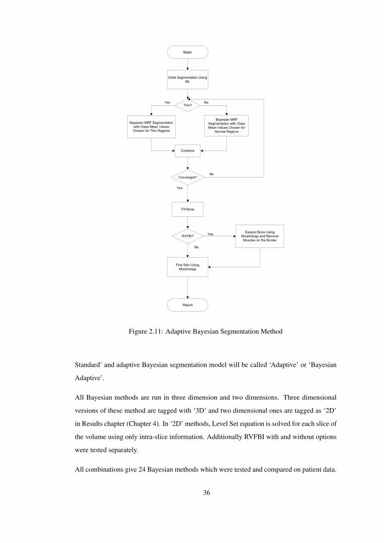
Begin

Yes

YesExpand Bone Using

Morphology and Remove

Muscles on the Border

Find Skin Using

Morphology

No

Converged?

RVFBI?

Combine

Bayesian MRF

Segmentation with Class

Mean Values Chosen for

Normal Regions

Bayesian MRF Segmentation

with Class Mean Values

Chosen for Thin Regions

Report

No

Fill Bone

Initial Segmentation Using

ML

Thin?Yes No

Figure 2.11: Adaptive Bayesian Segmentation Method

Standard’ and adaptive Bayesian segmentation model will be called ‘Adaptive’ or ‘Bayesian

Adaptive’.

All Bayesian methods are run in three dimension and two dimensions. Three dimensional

versions of these method are tagged with ‘3D’ and two dimensional ones are tagged as ‘2D’

in Results chapter (Chapter 4). In ‘2D’ methods, Level Set equation is solved for each slice of

the volume using only intra-slice information. Additionally RVFBI with and without options

were tested separately.

All combinations give 24 Bayesian methods which were tested and compared on patient data.

36

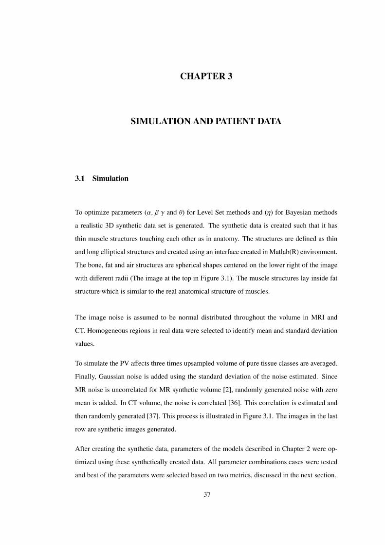
CHAPTER 3

SIMULATION AND PATIENT DATA

3.1 Simulation

To optimize parameters (α, β γ and θ) for Level Set methods and (η) for Bayesian methods

a realistic 3D synthetic data set is generated. The synthetic data is created such that it has

thin muscle structures touching each other as in anatomy. The structures are defined as thin

and long elliptical structures and created using an interface created in Matlab(R) environment.

The bone, fat and air structures are spherical shapes centered on the lower right of the image

with different radii (The image at the top in Figure 3.1). The muscle structures lay inside fat

structure which is similar to the real anatomical structure of muscles.

The image noise is assumed to be normal distributed throughout the volume in MRI and

CT. Homogeneous regions in real data were selected to identify mean and standard deviation

values.

To simulate the PV affects three times upsampled volume of pure tissue classes are averaged.

Finally, Gaussian noise is added using the standard deviation of the noise estimated. Since

MR noise is uncorrelated for MR synthetic volume [2], randomly generated noise with zero

mean is added. In CT volume, the noise is correlated [36]. This correlation is estimated and

then randomly generated [37]. This process is illustrated in Figure 3.1. The images in the last

row are synthetic images generated.

After creating the synthetic data, parameters of the models described in Chapter 2 were op-

timized using these synthetically created data. All parameter combinations cases were tested

and best of the parameters were selected based on two metrics, discussed in the next section.

37

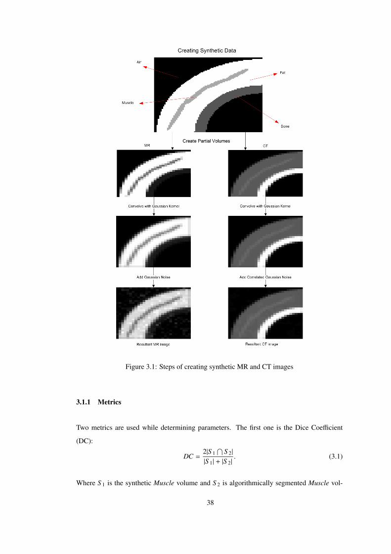
Figure 3.1: Steps of creating synthetic MR and CT images

3.1.1 Metrics

Two metrics are used while determining parameters. The first one is the Dice Coefficient

(DC):

DC =2|S 1

∩S 2|

|S 1| + |S 2|. (3.1)

Where S 1 is the synthetic Muscle volume and S 2 is algorithmically segmented Muscle vol-

38

ume. If they are the same volume, the DC takes the value of 1. Otherwise, it takes a value

between 0 and 1. The metric gives the ratio of overlapped volume to total volume of re-

gions. However, this metric does not provide information about boundary accuracy of the

segmentation.

The second metric used in this study compares boundaries of two label sets. It is called

Root Mean Squared Symmetric Surface Distance (RMSSSD). It measures symmetric distance

between two boundaries B1 and B2. The distance used in this study is Euclidian distance. The

metric is calculated as follows: First, calculate d1 = dist(B1, B2) and d2 = dist(B2, B1) where

d1 and d2 are squared symmetric distance arrays. di(k) (i = 1, 2; k ∈ Ni where Ni is the

number of voxels on boundary Bi) is the minimum distance of the voxel k which belongs to

set Bi to the boundary B j ( j , i). The d1 and d2 are combined to have d such that d is a vector.

Finally, d is root mean squared which gives RMSSSD. This metric gives small values if two

boundaries are close to each other. The metric is in Voxel units.

3.1.2 Parameter Optimization

The performance of each segmentation for a parameter set (α, β, γ and θ for Level Set methods

and η for Bayesian methods) on the simulated images is ranked using both DC and RMSSSD

metrics. It is a rating process:

1. Sort DC values in descending and RMSSSD values in ascending order.

2. Normalize all values such that:

• Minimum DC value becomes zero and maximum DC value becomes N (number

of parameter sets tested)

• Minimum RMSSD value becomes N and maximum RMSSD value becomes zero.

3. Add these values to obtain ratings.

4. Choose parameter set with the highest rating.

All of the optimum sets are determined using this procedure and used in evaluations on patient

data.

39

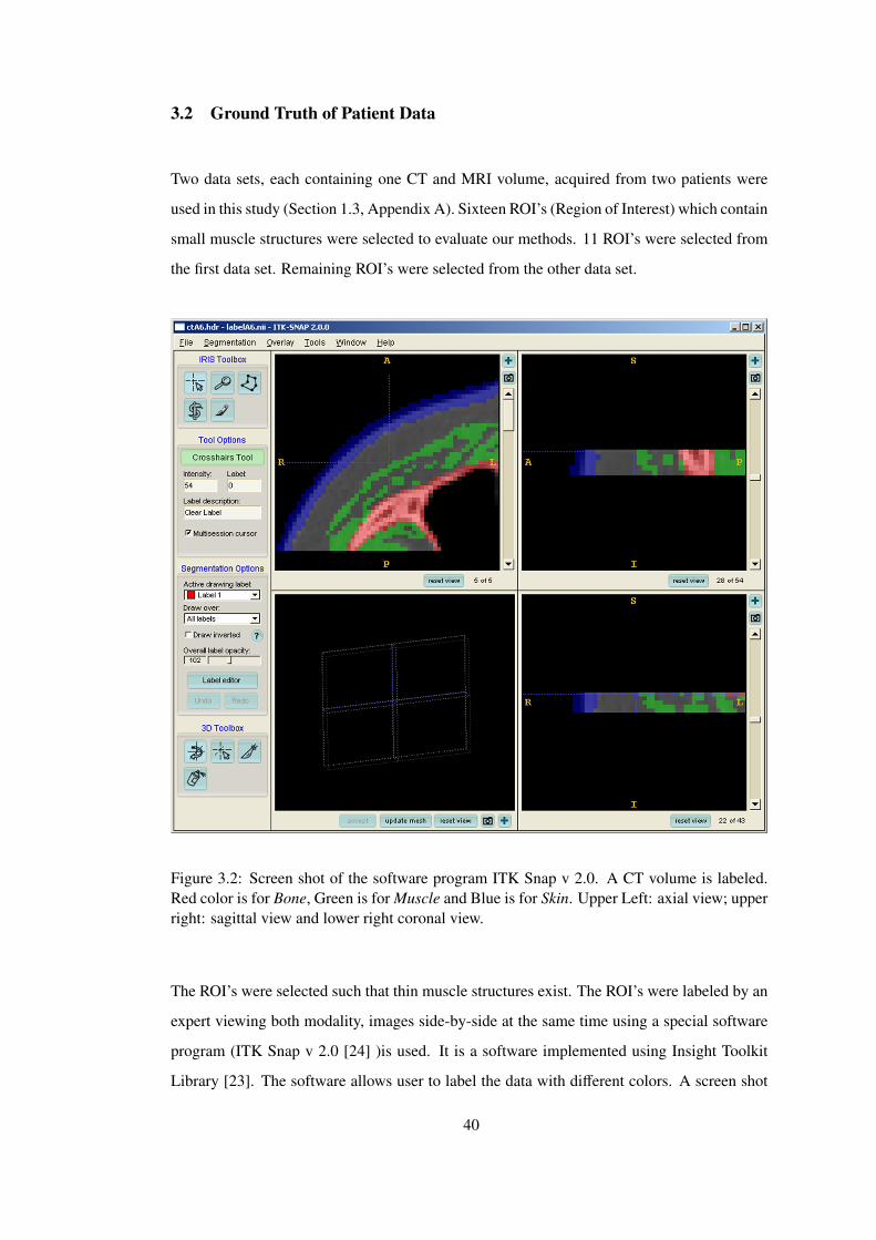
3.2 Ground Truth of Patient Data

Two data sets, each containing one CT and MRI volume, acquired from two patients were

used in this study (Section 1.3, Appendix A). Sixteen ROI’s (Region of Interest) which contain

small muscle structures were selected to evaluate our methods. 11 ROI’s were selected from

the first data set. Remaining ROI’s were selected from the other data set.

Figure 3.2: Screen shot of the software program ITK Snap v 2.0. A CT volume is labeled.Red color is for Bone, Green is for Muscle and Blue is for Skin. Upper Left: axial view; upperright: sagittal view and lower right coronal view.

The ROI’s were selected such that thin muscle structures exist. The ROI’s were labeled by an

expert viewing both modality, images side-by-side at the same time using a special software

program (ITK Snap v 2.0 [24] )is used. It is a software implemented using Insight Toolkit

Library [23]. The software allows user to label the data with different colors. A screen shot

40

of the software program is provided in Figure 3.2.

41

CHAPTER 4

RESULTS

4.1 Metrics and Statistical Analysis

The aim of this chapter is to quantitatively evaluate and compare the proposed methods by

using the hand-segmented images as ground truth. Two metrics are used while evaluating

methods as described in Section 3.1.1: The Dice Coefficient (DC) and Root Mean Squared

Symmetric Surface Distance (RMSSSD).

Using these metrics, methods are evaluated and compared using paired t-test. Two tailed and

one tailed paired t-tests are used. In two tailed test the null hypotheses H0 is that means of

two samples are equal. In one tailed test (depending on which tail is selected), the test is

performed against the hypotheses: The mean of the one sample is greater/smaller than the

other. The resulting statistics, p, is compared to the significance level (α). If p value is less

than α, the null hypotheses is rejected. In one tailed test, this means that one sample has

greater mean, and in two tailed test, it means that two samples have different means. α = 0.05

is selected in this study.

While deciding whether a method is better than the other, two paired t-tests are used on DC

and RMSSSD metric measurements. If the statistics of one of the metrics says two methods

have unequal means in two-tailed tests then, of the two metric, the one which has smaller p

value (one tailed test) is determined as a better result. The comparisons are made iteratively

between each pair of methods to determine the best method. In the following section these

statistical comparisons are given.

42

4.2 Comparison of Methods

While illustrating results two types of plot are used. The first one is mean ± standard deviation

graph. In horizontal axis every element corresponds to a method and y axis is the metric value.

The upper and lower limits are mean ± standard deviations and the dot in the middle represents

means of the metric. The second one is the metrics versus ROI’s. It shows what value metric

takes in that ROI (horizontal axis of the plot).

The best result is found by following steps. First, for every segmentation family (Bayesian

or Level Set), data groups (MR only, CT only and MR&CT cases) are evaluated within the

group. Then these three methods (one from MR only case, one from CT only case and one

from MR&CT unified case) are statistically compared and illustrated in figures. Finally, one

from Level Set family and one from Bayesian family is determined as best and compared to

each other.

There are 16 ROI’s and 60 methods and 2 metrics, so when giving the results only some re-

sults, figures and images are provided. In illustrations, methods with abbreviation ‘Y’ (Yes)

means RVFBI (Removing Voxels on the Fat Bone Interface) operation was applied. ‘N’ (No)

means RVFBI (Removing Voxels on the Fat Bone Interface) operation was not applied. ‘3D’

and ‘2D’ indicates whether the method operated slice-by-slice manner or using volumetric

information. In Level Set (LS) methods, abbreviation ‘Standard-p’ is used to name stan-

dard method using predefined class mean intensities and abbreviation ‘Standard-a’ is used

for standard method using automatically (in every iterations) calculated class mean intensities

and ‘Adaptive’ represents thickness adaptive Level Set model. Moreover, ‘FE’ stands for For-

ward Euler which represent forward euler time (explicit) solution of the Level Set equation.

Similarly, for Bayesian methods, ‘Standard’ is used for standard Bayesian and ‘Adaptive’ is

used for thickness adaptive model. See Section 2.3 and Section 2.4 for detailed explanation.

4.2.1 Bayesian with MRF Model Results

Figure 4.1 illustrates DC (Figure 4.1(a)) and RMSSSD (Figure 4.1(b))) metrics statistics

(means ± standard deviation) applied to MR data. In Figure 4.1(a), it is observed the methods

with RVFBI (‘Y’) have lower mean DC values than without RVFBI (‘N’) methods with no

noticeable change for RMSSSD metric (Figure 4.1(b)). This is related with an anatomical

43

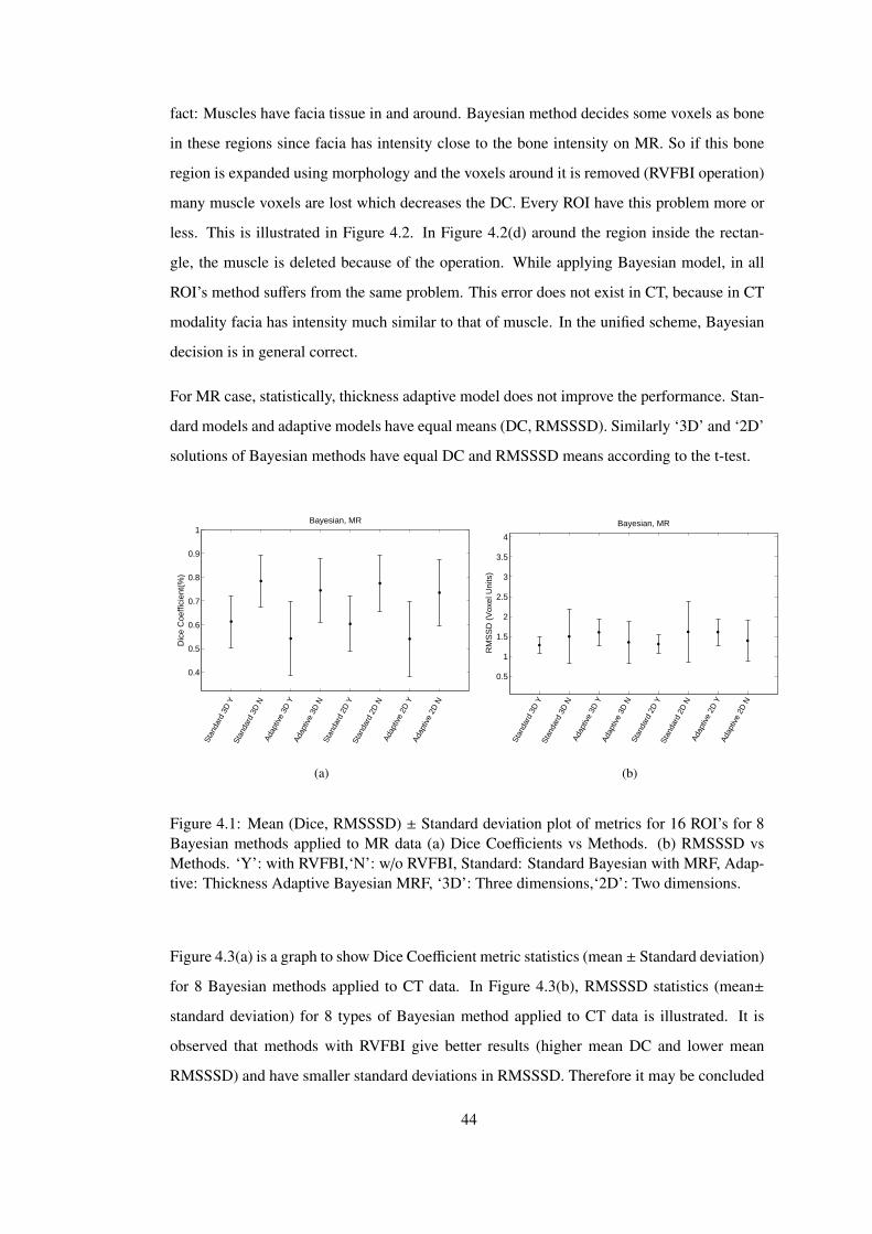
fact: Muscles have facia tissue in and around. Bayesian method decides some voxels as bone

in these regions since facia has intensity close to the bone intensity on MR. So if this bone

region is expanded using morphology and the voxels around it is removed (RVFBI operation)

many muscle voxels are lost which decreases the DC. Every ROI have this problem more or

less. This is illustrated in Figure 4.2. In Figure 4.2(d) around the region inside the rectan-

gle, the muscle is deleted because of the operation. While applying Bayesian model, in all

ROI’s method suffers from the same problem. This error does not exist in CT, because in CT

modality facia has intensity much similar to that of muscle. In the unified scheme, Bayesian

decision is in general correct.

For MR case, statistically, thickness adaptive model does not improve the performance. Stan-

dard models and adaptive models have equal means (DC, RMSSSD). Similarly ‘3D’ and ‘2D’

solutions of Bayesian methods have equal DC and RMSSSD means according to the t-test.

0.4

0.5

0.6

0.7

0.8

0.9

1Bayesian, MR

Dic

e C

oeffi

cien

t(%

)

Stan

dard

3D

YSt

anda

rd 3

D N

Adap

tive

3D Y

Adap

tive

3D N

Stan

dard

2D

YSt

anda

rd 2

D N

Adap

tive

2D Y

Adap

tive

2D N

(a)

0.5

1

1.5

2

2.5

3

3.5

4

Bayesian, MR

RM

SS

D (

Vox

el U

nits

)

Stan

dard

3D

YSt

anda

rd 3

D N

Adap

tive

3D Y

Adap

tive

3D N

Stan

dard

2D

YSt

anda

rd 2

D N

Adap

tive

2D Y

Adap

tive

2D N

(b)

Figure 4.1: Mean (Dice, RMSSSD) ± Standard deviation plot of metrics for 16 ROI’s for 8Bayesian methods applied to MR data (a) Dice Coefficients vs Methods. (b) RMSSSD vsMethods. ‘Y’: with RVFBI,‘N’: w/o RVFBI, Standard: Standard Bayesian with MRF, Adap-tive: Thickness Adaptive Bayesian MRF, ‘3D’: Three dimensions,‘2D’: Two dimensions.

Figure 4.3(a) is a graph to show Dice Coefficient metric statistics (mean ± Standard deviation)

for 8 Bayesian methods applied to CT data. In Figure 4.3(b), RMSSSD statistics (mean±

standard deviation) for 8 types of Bayesian method applied to CT data is illustrated. It is

observed that methods with RVFBI give better results (higher mean DC and lower mean

RMSSSD) and have smaller standard deviations in RMSSSD. Therefore it may be concluded

44

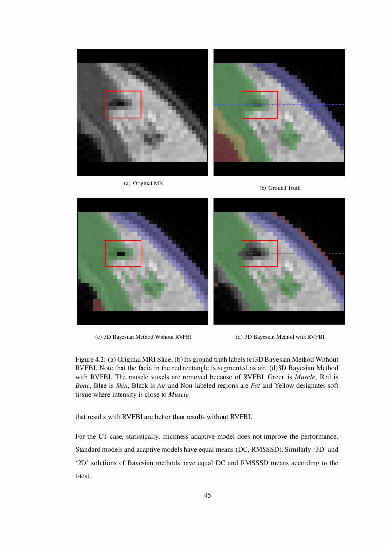
(a) Original MR(b) Ground Truth

(c) 3D Bayesian Method Without RVFBI (d) 3D Bayesian Method with RVFBI

Figure 4.2: (a) Original MRI Slice, (b) Its ground truth labels (c)3D Bayesian Method WithoutRVFBI, Note that the facia in the red rectangle is segmented as air. (d)3D Bayesian Methodwith RVFBI. The muscle voxels are removed because of RVFBI. Green is Muscle, Red isBone, Blue is Skin, Black is Air and Non-labeled regions are Fat and Yellow designates softtissue where intensity is close to Muscle

that results with RVFBI are better than results without RVFBI.

For the CT case, statistically, thickness adaptive model does not improve the performance.

Standard models and adaptive models have equal means (DC, RMSSSD). Similarly ‘3D’ and

‘2D’ solutions of Bayesian methods have equal DC and RMSSSD means according to the

t-test.

45

0.4

0.5

0.6

0.7

0.8

0.9

1Bayesian, CT

Dic

e C

oeffi

cien

t(%

)

Stan

dard

3D

YSt

anda

rd 3

D N

Adap

tive

3D Y

Adap

tive

3D N

Stan

dard

2D

YSt

anda

rd 2

D N

Adap

tive

2D Y

Adap

tive

2D N

(a)

0.5

1

1.5

2

2.5

3

3.5

4

Bayesian, CT

RM

SS

D (

Vox

el U

nits

)

Stan

dard

3D

YSt

anda

rd 3

D N

Adap

tive

3D Y

Adap

tive

3D N

Stan

dard

2D

YSt

anda

rd 2

D N

Adap

tive

2D Y

Adap

tive

2D N

(b)

Figure 4.3: Mean (Dice, RMSSSD) ± Standard deviation for 8 Bayesian methods applied toCT data (a) Dice Coefficients vs Methods. (b) RMSSSD vs Methods. Figure descriptions aresame as Figure 4.1

Statistically best results for only MR (Figure 4.1) and only CT (Figure 4.3) case are as follows

(also see Figure 4.5):

• For CT only:

– Standard 3D Bayesian Method with RVFBI,

– Adaptive 3D Bayesian Method with RVFBI,

– Standard 2D Bayesian Method with RVFBI,

– Adaptive 2D Bayesian Method with RVFBI,

• For MR only: Adaptive 3D Bayesian Model without RVFBI,

– Standard 3D Bayesian Method without RVFBI,

– Adaptive 3D Bayesian Method without RVFBI,

– Standard 2D Bayesian Method without RVFBI,

– Adaptive 2D Bayesian Method without RVFBI.

But none of the RMSSSD and DC metrics means of these two data cases are statistically

different. In an example, paired t-test which compared Standard 3D Bayesian Method with

RVFBI for CT case gave pDC = 0.1204 > 0.05 and pRMS S S D = 0.8960 > 0.05. This means

that there is no difference in using MR or CT alone if one type of modality is available.

46

Figure 4.4(a) and Figure 4.4(b) depicts DC and RMSSSD metrics statistics for 8 Bayesian

methods applied to MR&CT unified data. Results with RVFBI give better means and less

variations.

For unified data case, statistically, thickness adaptive model does not improve the perfor-

mance. Standard models and adaptive models have equal means (DC, RMSSSD). Similarly

‘3D’ and ‘2D’ solutions of Bayesian methods have equal DC and RMSSSD means according

to the t-test.

Most successful methods are:

• Standard 3D Bayesian Model with RVFBI,

• Adaptive 3D Bayesian Model with RVFBI,

• Standard 2D Bayesian Model with RVFBI,

• Adaptive 2D Bayesian Model with RVFBI.

0.4

0.5

0.6

0.7

0.8

0.9

1Bayesian, MR&CT

Dic

e C

oeffi

cien

t(%

)

Stan

dard

3D

YSt

anda

rd 3

D N

Adap

tive

3D Y

Adap

tive

3D N

Stan

dard

2D

YSt

anda

rd 2

D N

Adap

tive

2D Y

Adap

tive

2D N

(a)

0.5

1

1.5

2

2.5

3

3.5

4

Bayesian, MR&CT

RM

SS

D (

Vox

el U

nits

)

Stan

dard

3D

YSt

anda

rd 3

D N

Adap

tive

3D Y

Adap

tive

3D N

Stan

dard

2D

YSt

anda

rd 2

D N

Adap

tive

2D Y

Adap

tive

2D N

(b)

Figure 4.4: Mean (Dice, RMSSSD) ± Standard deviation for 8 Bayesian methods applied toMR&CT data (a) Dice Coefficients vs Methods. (b) RMSSSD vs Methods. Figure descrip-tions are same as Figure 4.1

Two tailed t-tests shows that RMSSSD and DC means of these four methods are not statisti-

cally different (Table 4.1) but the 3D Adaptive case with RVFBI is chosen to be the best model

with the comparison rule described in the beginning of this section. It can be concluded that

47

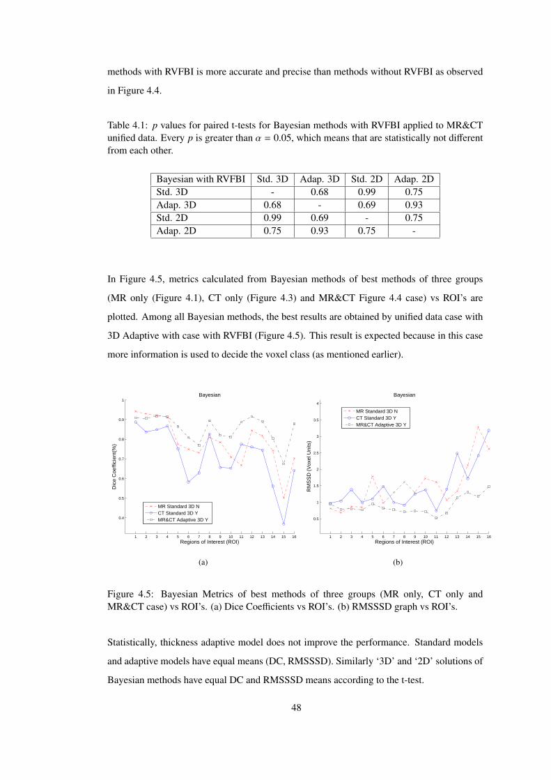
methods with RVFBI is more accurate and precise than methods without RVFBI as observed

in Figure 4.4.

Table 4.1: p values for paired t-tests for Bayesian methods with RVFBI applied to MR&CTunified data. Every p is greater than α = 0.05, which means that are statistically not differentfrom each other.

Bayesian with RVFBI Std. 3D Adap. 3D Std. 2D Adap. 2DStd. 3D - 0.68 0.99 0.75Adap. 3D 0.68 - 0.69 0.93Std. 2D 0.99 0.69 - 0.75Adap. 2D 0.75 0.93 0.75 -

In Figure 4.5, metrics calculated from Bayesian methods of best methods of three groups

(MR only (Figure 4.1), CT only (Figure 4.3) and MR&CT Figure 4.4 case) vs ROI’s are

plotted. Among all Bayesian methods, the best results are obtained by unified data case with

3D Adaptive with case with RVFBI (Figure 4.5). This result is expected because in this case

more information is used to decide the voxel class (as mentioned earlier).

1 2 3 4 5 6 7 8 9 10 11 12 13 14 15 16

0.4

0.5

0.6

0.7

0.8

0.9

1

Dic

e C

oeffi

cien

t(%

)

Bayesian

Regions of Interest (ROI)

MR Standard 3D NCT Standard 3D YMR&CT Adaptive 3D Y

(a)

1 2 3 4 5 6 7 8 9 10 11 12 13 14 15 16

0.5

1

1.5

2

2.5

3

3.5

4

RM

SS

D (

Vox

el U

nits

)

Bayesian

Regions of Interest (ROI)

MR Standard 3D NCT Standard 3D YMR&CT Adaptive 3D Y

(b)

Figure 4.5: Bayesian Metrics of best methods of three groups (MR only, CT only andMR&CT case) vs ROI’s. (a) Dice Coefficients vs ROI’s. (b) RMSSSD graph vs ROI’s.

Statistically, thickness adaptive model does not improve the performance. Standard models

and adaptive models have equal means (DC, RMSSSD). Similarly ‘3D’ and ‘2D’ solutions of

Bayesian methods have equal DC and RMSSSD means according to the t-test.

48

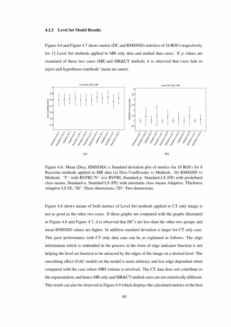
4.2.2 Level Set Model Results

Figure 4.6 and Figure 4.7 shows metric (DC and RMSSSD) statistics of 16 ROI’s respectively,

for 12 Level Set methods applied to MR only data and unified data cases. If p values are

examined of these two cases (MR and MR&CT unified), it is observed that t-test fails to

reject null hypotheses (methods’ mean are same).

0.4

0.5

0.6

0.7

0.8

0.9

1Level Set (FE), MR

Dic

e C

oeffi

cien

t(%

)St

anda

rd−p

3D

YSt

anda

rd−p

3D

NAd

aptiv

e 3D

YAd

aptiv

e 3D

NSt

anda

rd−a

3D

YSt

anda

rd−a

3D

NSt

anda

rd−p

2D

YSt

anda

rd−p

2D

NAd

aptiv

e 2D

YAd

aptiv

e 2D

NSt

anda

rd−a

2D

YSt

anda

rd−a

2D

N

(a)

0.5

1

1.5

2

2.5

3

3.5

4

Level Set (FE), MR

RM

SS

D (

Vox

el U

nits

)St

anda

rd−p

3D

YSt

anda

rd−p

3D

NAd

aptiv

e 3D

YAd

aptiv

e 3D

NSt

anda

rd−a

3D

YSt

anda

rd−a

3D

NSt

anda

rd−p

2D

YSt

anda

rd−p

2D

NAd

aptiv

e 2D

YAd

aptiv

e 2D

NSt

anda

rd−a

2D

YSt

anda

rd−a

2D

N

(b)

Figure 4.6: Mean (Dice, RMSSSD) ± Standard deviation plot of metrics for 16 ROI’s for 8Bayesian methods applied to MR data (a) Dice Coefficients vs Methods. (b) RMSSSD vsMethods. ‘Y’: with RVFBI,‘N’: w/o RVFBI, Standard-p: Standard LS (FE) with predefinedclass means, Standard-a: Standard LS (FE) with automatic class means Adaptive: ThicknessAdaptive LS FE,‘3D’: Three dimensions,‘2D’: Two dimensions.

Figure 4.8 shows means of both metrics of Level Set methods applied to CT only image is

not as good as the other two cases. If these graphs are compared with the graphs illustrated

in Figure 4.6 and Figure 4.7, it is observed that DC’s are less than the other two groups and

mean RMSSSD values are higher. In addition standard deviation is larger for CT only case.

This poor performance with CT only data case can be as explained as follows: The edge

information which is embedded in the process in the form of edge indicator function is not

helping the level set function to be attracted by the edges of the image on a desired level. The

smoothing effect (GAC model) on the model is more arbitrary and less edge dependent when

compared with the case where MRI volume is involved. The CT data does not contribute to

the segmentation, and hence MR only and MR&CT unified cases are not statistically different.

This result can also be observed in Figure 4.9 which displays the calculated metrics of the best

49

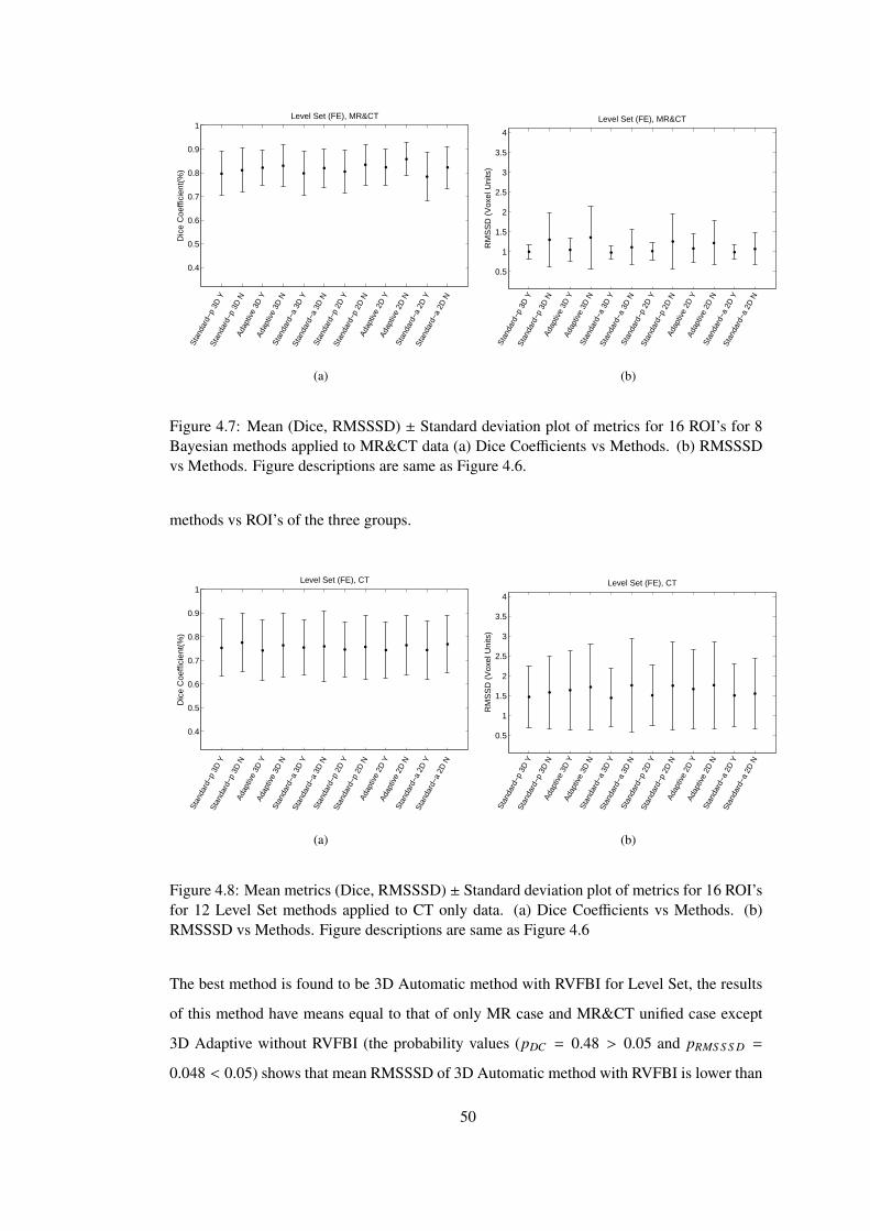
0.4

0.5

0.6

0.7

0.8

0.9

1Level Set (FE), MR&CT

Dic

e C

oeffi

cien

t(%

)St

anda

rd−p

3D

YSt

anda

rd−p

3D

NAd

aptiv

e 3D

YAd

aptiv

e 3D

NSt

anda

rd−a

3D

YSt

anda

rd−a

3D

NSt

anda

rd−p

2D

YSt

anda

rd−p

2D

NAd

aptiv

e 2D

YAd

aptiv

e 2D

NSt

anda

rd−a

2D

YSt

anda

rd−a

2D

N

(a)

0.5

1

1.5

2

2.5

3

3.5

4

Level Set (FE), MR&CT

RM

SS

D (

Vox

el U

nits

)St

anda

rd−p

3D

YSt

anda

rd−p

3D

NAd

aptiv

e 3D

YAd

aptiv

e 3D

NSt

anda

rd−a

3D

YSt

anda

rd−a

3D

NSt

anda

rd−p

2D

YSt

anda

rd−p

2D

NAd

aptiv

e 2D

YAd

aptiv

e 2D

NSt

anda

rd−a

2D

YSt

anda

rd−a

2D

N

(b)

Figure 4.7: Mean (Dice, RMSSSD) ± Standard deviation plot of metrics for 16 ROI’s for 8Bayesian methods applied to MR&CT data (a) Dice Coefficients vs Methods. (b) RMSSSDvs Methods. Figure descriptions are same as Figure 4.6.

methods vs ROI’s of the three groups.

0.4

0.5

0.6

0.7

0.8

0.9

1Level Set (FE), CT

Dic

e C

oeffi

cien

t(%

)St

anda

rd−p

3D

YSt

anda

rd−p

3D

NAd

aptiv

e 3D

YAd

aptiv

e 3D

NSt

anda

rd−a

3D

YSt

anda

rd−a

3D

NSt

anda

rd−p

2D

YSt

anda

rd−p

2D

NAd

aptiv

e 2D

YAd

aptiv

e 2D

NSt

anda

rd−a

2D

YSt

anda

rd−a

2D

N

(a)

0.5

1

1.5

2

2.5

3

3.5

4

Level Set (FE), CT

RM

SS

D (

Vox

el U

nits

)St

anda

rd−p

3D

YSt

anda

rd−p

3D

NAd

aptiv

e 3D

YAd

aptiv

e 3D

NSt

anda

rd−a

3D

YSt

anda

rd−a

3D

NSt

anda

rd−p

2D

YSt

anda

rd−p

2D

NAd

aptiv

e 2D

YAd

aptiv

e 2D

NSt

anda

rd−a

2D

YSt

anda

rd−a

2D

N

(b)

Figure 4.8: Mean metrics (Dice, RMSSSD) ± Standard deviation plot of metrics for 16 ROI’sfor 12 Level Set methods applied to CT only data. (a) Dice Coefficients vs Methods. (b)RMSSSD vs Methods. Figure descriptions are same as Figure 4.6

The best method is found to be 3D Automatic method with RVFBI for Level Set, the results

of this method have means equal to that of only MR case and MR&CT unified case except

3D Adaptive without RVFBI (the probability values (pDC = 0.48 > 0.05 and pRMS S S D =

0.048 < 0.05) shows that mean RMSSSD of 3D Automatic method with RVFBI is lower than

50

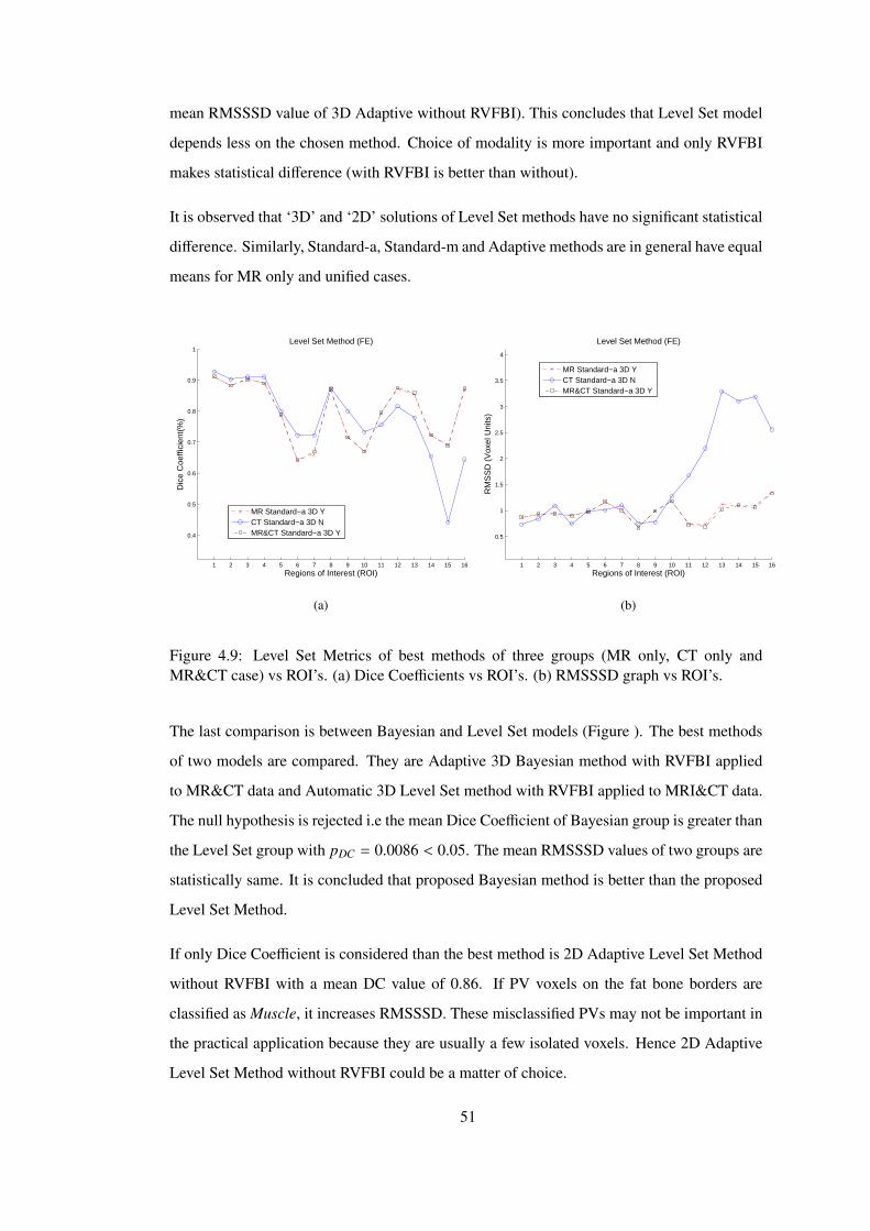
mean RMSSSD value of 3D Adaptive without RVFBI). This concludes that Level Set model

depends less on the chosen method. Choice of modality is more important and only RVFBI

makes statistical difference (with RVFBI is better than without).

It is observed that ‘3D’ and ‘2D’ solutions of Level Set methods have no significant statistical

difference. Similarly, Standard-a, Standard-m and Adaptive methods are in general have equal

means for MR only and unified cases.

1 2 3 4 5 6 7 8 9 10 11 12 13 14 15 16

0.4

0.5

0.6

0.7

0.8

0.9

1

Dic

e C

oeffi

cien

t(%

)

Level Set Method (FE)

Regions of Interest (ROI)

MR Standard−a 3D YCT Standard−a 3D NMR&CT Standard−a 3D Y

(a)

1 2 3 4 5 6 7 8 9 10 11 12 13 14 15 16

0.5

1

1.5

2

2.5

3

3.5

4

RM

SS

D (

Vox

el U

nits

)

Level Set Method (FE)

Regions of Interest (ROI)

MR Standard−a 3D YCT Standard−a 3D NMR&CT Standard−a 3D Y

(b)

Figure 4.9: Level Set Metrics of best methods of three groups (MR only, CT only andMR&CT case) vs ROI’s. (a) Dice Coefficients vs ROI’s. (b) RMSSSD graph vs ROI’s.

The last comparison is between Bayesian and Level Set models (Figure ). The best methods

of two models are compared. They are Adaptive 3D Bayesian method with RVFBI applied

to MR&CT data and Automatic 3D Level Set method with RVFBI applied to MRI&CT data.

The null hypothesis is rejected i.e the mean Dice Coefficient of Bayesian group is greater than

the Level Set group with pDC = 0.0086 < 0.05. The mean RMSSSD values of two groups are

statistically same. It is concluded that proposed Bayesian method is better than the proposed

Level Set Method.

If only Dice Coefficient is considered than the best method is 2D Adaptive Level Set Method

without RVFBI with a mean DC value of 0.86. If PV voxels on the fat bone borders are

classified as Muscle, it increases RMSSSD. These misclassified PVs may not be important in

the practical application because they are usually a few isolated voxels. Hence 2D Adaptive

Level Set Method without RVFBI could be a matter of choice.

51

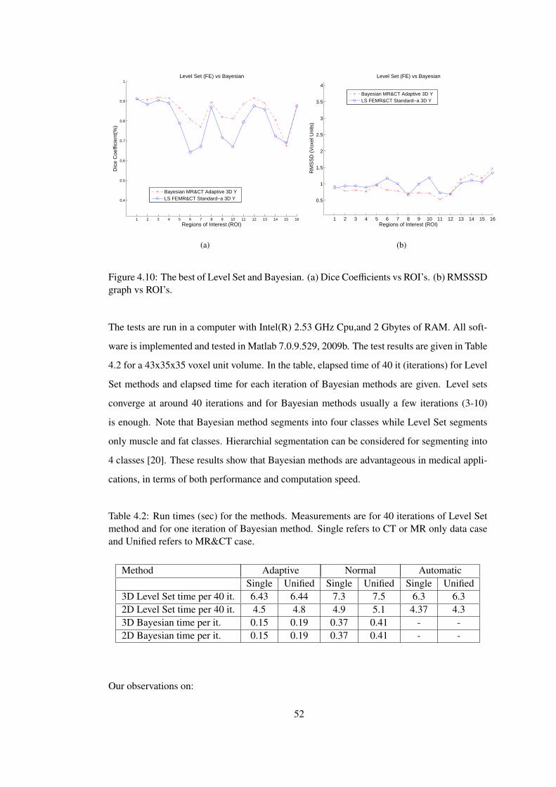
1 2 3 4 5 6 7 8 9 10 11 12 13 14 15 16

0.4

0.5

0.6

0.7

0.8

0.9

1

Dic

e C

oeffi

cien

t(%

)

Level Set (FE) vs Bayesian

Regions of Interest (ROI)

Bayesian MR&CT Adaptive 3D YLS FEMR&CT Standard−a 3D Y

(a)

1 2 3 4 5 6 7 8 9 10 11 12 13 14 15 16

0.5

1

1.5

2

2.5

3

3.5

4

RM

SS

D (

Vox

el U

nits

)

Level Set (FE) vs Bayesian

Regions of Interest (ROI)

Bayesian MR&CT Adaptive 3D YLS FEMR&CT Standard−a 3D Y

(b)

Figure 4.10: The best of Level Set and Bayesian. (a) Dice Coefficients vs ROI’s. (b) RMSSSDgraph vs ROI’s.

The tests are run in a computer with Intel(R) 2.53 GHz Cpu,and 2 Gbytes of RAM. All soft-

ware is implemented and tested in Matlab 7.0.9.529, 2009b. The test results are given in Table

4.2 for a 43x35x35 voxel unit volume. In the table, elapsed time of 40 it (iterations) for Level

Set methods and elapsed time for each iteration of Bayesian methods are given. Level sets

converge at around 40 iterations and for Bayesian methods usually a few iterations (3-10)

is enough. Note that Bayesian method segments into four classes while Level Set segments

only muscle and fat classes. Hierarchial segmentation can be considered for segmenting into

4 classes [20]. These results show that Bayesian methods are advantageous in medical appli-

cations, in terms of both performance and computation speed.

Table 4.2: Run times (sec) for the methods. Measurements are for 40 iterations of Level Setmethod and for one iteration of Bayesian method. Single refers to CT or MR only data caseand Unified refers to MR&CT case.

Method Adaptive Normal AutomaticSingle Unified Single Unified Single Unified

3D Level Set time per 40 it. 6.43 6.44 7.3 7.5 6.3 6.32D Level Set time per 40 it. 4.5 4.8 4.9 5.1 4.37 4.33D Bayesian time per it. 0.15 0.19 0.37 0.41 - -2D Bayesian time per it. 0.15 0.19 0.37 0.41 - -

Our observations on:

52

• 2D vs 3D method results: In general no statistical difference is found between these

two type of approaches.

• Methods with vs without RVFBI: In general methods with RVFBI gives better results

except for the Bayesian MR case (because of the facia tissue inside and around the

muscles).

• Three data cases: Bayesian methods gives better results in unified case. Bests of MR

only and CT only cases are statistically same. Level Set methods gives equal results for

MR only and MR&CT unifed case. which are better than CT methods.

53

CHAPTER 5

CONCLUSIONS AND FUTURE WORK

5.1 Conclusion and Discussion

In this thesis the aim was to segment thin muscle structures using two types of segmentation

models: Geodesic Active Contour Level Sets and Bayesian Markov Random Field with Partial

Volume. These models have standard and thickness adaptive versions. They were applied

for three data cases: MR only, CT only and MR&CT unified. Additionally, 3D and 2D

versions of these methods were applied. In adaptive models, thickness of muscle structures

were detected and class means were tuned for thin regions. These models included preprocess

and postprocess steps (which contains simple image processing routines like morphological

operations). Postprocess includes RVFBI (Removing Voxels on the Fat Bone Interface) which

was considered an optional step, and skin removal.

For Level Set, Geodesic Active Contour model was used. It has a term minimizing inte-

gral of edge indicator function over the level set boundary, and it uses Chan-Vese model to

find smooth regions. This model often stops in the local minima. In this study, a K-means

initialization algorithm was used to prevent this, which provides a quicker convergence time.

Moreover, a simulation study was designed to optimize free parameters (α, β, γ and θ for

Level Set and η for Bayesian) of methods in all combinations of 2D, 3D; with or without

RVFBI; standard-a, standard-p, adaptive for Level Sets and standard, adaptive for Bayesian;

CT only, MR only and unified (MR&CT) cases. To optimize these parameters, a synthetic

data set (including an MR and CT volume) was created. Proposed methods were applied with

different set of parameters to choose the best parameter set optimizing two metrics.

MR and CT data was hand-segmented by an expert radiologist to create ground truth. Pro-

54

posed automatic segmentation method results were compared with ground truth data using

Dice Coefficient (to measure volumetric segmentation accuracy) and Root Mean Squared

Symmetric Surface Distance (to measure boundary segmentation accuracy). These metrics

were compared statistically (using t-test) to determine the best method.

The 3D Adaptive Bayesian method with RVFBI applied on MR&CT unified case was ob-

served to be the best method among Bayesian methods, however it is not statistically different

from other Bayesian methods with RVFBI. Additionally, Bayesian MR&CT cases are better

than individual image cases (MR only and CT only). It can be concluded that unifying data

and RVFBI creates statistical difference for Bayesian segmentation model.

For the Level Set model, the best case is 3D Auto Level Set model with RVFBI using MR&CT

unified case. Though, this model is found to be statistically no different from methods applied

on MR case or unified data cases.

CT Level Set model resulted in the worst performance. We believe that the reason is that CT

edge information does not contribute to the muscle segmentation model a lot. But in Level

Set model CT is necessary in preprocessing operations to remove air and bone tissues (in CT

images bone and air contrast is better than MR images).

Final comparison was made between the best Bayesian (3D adaptive with RVFBI applied on

MR&CT) and the best Level Set (3D standard-a with RVFBI applied on MR&CT) methods.

Bayesian method have higher Dice Coefficient mean than Level Set model (RMSSSD means

of both groups are not different). Therefore we conclude that the Bayesian model is better

than the Level Set in segmentation performance.

In addition, unified (MR&CT) data provides better segmentation accuracy as compared with

single modality cases. However this depends on image registration accuracy. In fact, in

our second data set, we observed some problems in CT-MR registration even with non-rigid

techniques. This is why less number of ROI’s were selected from second data set.

Moreover, our observations on 3D and 2D shows that these approaches are not statistically

different. Similarly, adaptive methods are not better than standard methods, statistically.

Run times were also compared. The convergence time for the Level Set method was much

higher than the Bayesian methods. Moreover, Bayesian model segments images into four

55

classes, while Level Set model segments images into only two classes.

5.2 Future Work

Our measurements have shown that Bayesian methods converge faster than the Level Set

methods. However Fast Marching algorithm [26] and GPU programming techniques can be

used [38] to improve Level Set computation time.

To improve Level Set Segmentation performance, initialization independent methods which

provides global minimization to the geodesic active contour model can be considered [39].

Improving edge information and modifying or changing the minimum variance term with a

more efficient term [40] may also improve segmentation results. Hierarchical methods [20]

can be used to segment all four classes which may improve the results. It is also possible to

use air and bone segmentation results of Bayesian method to obtain a better air-bone mask.

To improve Bayesian segmentation performance prior models other than Gibb’s prior can be

explored.

Our methods (both Bayesian and Level Set) did not account for the differences in image

resolution between MR and CT volumes. It is necessary to develop techniques to take into

account resolution differences.

In addition, our tests were on two patient only. This is obviously not sufficient. Algorithm

training on separate data set can be preferred.

Knowledge based supervised algorithms can also be considered for further improvements

like [41]. However, human facial anatomy is very complex and there is wide variability along

population which hinders generation of a statistical atlas.

Semi-automated methods are necessary to separate non-muscle tissue (glands and vessels)

from the muscle class.

In this thesis, the effect of MR and CT artifacts due to implants and fillings was not investi-

gated, and the subject of future studies.

56

REFERENCES

[1] Tubitak 1001, Proje No: 105E128, “Farklı goruntuleme tekniklerinin birlestirilmesiile kisiye Ozel sert ve yumusak doku ile kisinin dıs gorunumunu Iceren 3b kafamodellenmesi ve bu modelin 3b gorsellestirilmesi,” tech. rep., TUBITAK, 2008.

[2] D. W. Shattuck, S. R. Sandor-Leahy, K. A. Schaper, D. A. Rottenberg, and R. M.Leahy, “Magnetic resonance image tissue classification using a partial volume model,”NeuroImage, vol. 13, pp. 856–876, 2001.

[3] T. Tasdizen, D. Weinstein, and J. N. Lee, “Automatic tissue classification for the humanhead from multispectral MRI,” tech. rep., UCLA, 2004.

[4] “SCIRun: A scientific computing problem solving environment, scientific computingand imaging institute (SCI).”

[5] R. Olszewski, Y. Liu, T. Duprez, T. Xu, and H. Reychler, “Three-dimensional appear-ance of the lips muscles with three-dimensional isotropic MRI: in vivo study.,” Int JComput Assist Radiol Surg., vol. 4, pp. 349–52, 2009 Jun.

[6] E. Gladilin, S. Zachow, P. Deuflhard, and H. Hege, “Anatomy and physics-based facialanimation for craniofacial surgery simulations,” Medical & Biological Engineering &Computing, vol. 42(2), pp. pp 167–170, 2004.

[7] Y. Kang, K. Engelke, and W. A. Kalender, “Interactive 3d editing tools for imagesegmentation,” Medical Image Analysis, vol. 8, no. 1, pp. 35 – 46, 2004.

[8] S. Beucher and C. D. M. Mathmatique, “The watershed transformation applied to imagesegmentation,” in Scanning Microscopy International, pp. 299–314, 1991.

[9] N. R. Pal and S. K. . Pal, “A review in image segmentation techniques,” PatternRecognition, vol. 26, pp. 1277–1294, 1993.

[10] R. Adams and L. Bischof, “Seeded region growing,” IEEE Trans. Pattern Anal. Mach.Intell., vol. 16, no. 6, pp. 641–647, 1994.

57

[11] N. Pal and S. Pal, “A review on image segmentation techniques,” Pattern Recognition,vol. 26, no. 9, pp. 1277–1294, 1993.

[12] E. C. Hildreth, “Theory of edge detection,” Proceedings of the Royal Society of London.Series, vol. 207, pp. 187–217, 1985.

[13] S. Osher and J. A. Sethian, “Fronts propagating with curvature dependent speed: Al-gorithms based on hamilton-jacobi formulations,” Journal Of Computational Physics,vol. 79, no. 1, pp. 12–49, 1988.

[14] D. Mumford and J. Shah, “Optimal approximations by piecewise smooth functions andvariational problems,” CPAM, vol. XLII, no. 5, pp. 577–685, 1988.

[15] T. Chan and L. Vese, “Active contours without edges,” Image Processing, IEEETransactions on, vol. 10, pp. 266 –277, feb 2001.

[16] V. Caselles, F. Catte, T. Coll, and F. Dibos, “A geometric model for active contours inimage processing,” NumMath, vol. 66, pp. 1–31, 1993.

[17] R. Malladi, J. A. Sethian, and B. C. Vemuri, “Evolutionary fronts for topology-independent shape modeling and recovery,” in ECCV ’94: Proceedings of the thirdEuropean conference on Computer vision (vol. 1), (Secaucus, NJ, USA), pp. 3–13,Springer-Verlag New York, Inc., 1994.

[18] V. Caselles, R. Kimmel, and G. Sapiro, “Geodesic active contours,” InternationalJournal of Computer Vision, vol. 22, pp. 61–79, 1995.

[19] R. Kimmel, “Fast edge integration,” 2003.

[20] M. Holtzman Gazit, R. Kimmel, N. Peled, and D. Goldsher, “Segmentation of thinstructures in volumetric medical images,” IP, vol. 15, pp. 354–363, February 2006.

[21] J. B. G. Xiao, J. Noble, M. Burcher, and R.English, “Nonrigid registration of 3-dfree-hand ultrasound images of the breast,” IEEE Transactions on Medical Imaging,vol. Volume 21, No. 4, pp. 405–412, 2002.

[22] N. Tustison, “N3 algorithm explanation:http://www.midasjournal.org/browse/publication/640.”

[23] L. Ibanez, W. Schroeder, L. Ng, and J. Cates, The ITK Software Guide. Kitware, Inc.ISBN 1-930934-10-6, http://www.itk.org/ItkSoftwareGuide.pdf, first ed., 2003.

58

[24] P. A. Yushkevich, J. Piven, H. Cody Hazlett, R. Gimpel Smith, S. Ho, J. C. Gee,and G. Gerig, “User-guided 3D active contour segmentation of anatomical structures:Significantly improved efficiency and reliability,” Neuroimage, vol. 31, no. 3, pp. 1116–1128, 2006.

[25] M. Kass, A. Witkin, and D. Terzopoulos, “Snakes: Active contour models,” Interna-tional Journal Of Computer Vision, vol. 1, no. 4, pp. 321–331, 1988.

[26] J. A. Sethian, Level Set Methods and Fast Marching Methods. Cambridge UniversityPress, 1999.

[27] S. Osher and R. Fedkiw, Level Set Methods and Dynamic Implicit Surfaces. Springer,2002.

[28] X.-D. Liu, S. Osher, and T. Chan, “Weighted essentially non-oscillatory schemes,” 1994.

[29] G.-S. Jiang, C.-W. Shu, and I. L, “Efficient implementation of weighted eno schemes,”J. Comput. Phys, vol. 126, pp. 202–228, 1995.

[30] G.-S. Jiang and D. Peng, “Weighted eno schemes for hamilton–jacobi equations,” SIAMJ. Sci. Comput., vol. 21, no. 6, pp. 2126–2143, 1999.

[31] R. P. Fedkiw, B. Merriman, and S. Osher, “Efficient characteristic projection in upwinddifference schemes for hyperbolic systems (the complementary projection method,” J.Computational Physics, vol. 141, pp. 22–36, 1998.

[32] C. P. Lee, Robust Image Segmentation using Active Contours: Level Set Approaches.PhD thesis, Department of Electrical and Computer Engineering North Carolina StateUniversity, 2005.

[33] E. Kreyszig, Differential Geometry. University of Toronto Press, 1959.

[34] F. E. Eric, F. Gibou, and R. Fedkiw, “A fast hybrid k-means level set algorithm forsegmentation,” tech. rep., 4th Annual Hawaii International Conference on Statistics andMathematics, 2002.

[35] E. Sener, E. Mumcuoglu, E. Kale, and V. Akgun, “BT ve MR goruntulerini 3 boyuttaCakıstırarak ve birlikte kullanarak, otomatik ve yarı-otomatik bolutleme yontemlerigelistirilmesi ve bu yontemlerin kafa modeli olusturma ve yuz mimik kaslarınınbolutlenmesine uygulanması,” in 5. Ulusal Tıp Bilisimi Kongresi/Medical InformaticsTurkey, 2008.

59

[36] P. Razifar, M. Sandstrom, H. Schnieder, B. Langstrom, E. Maripuu, E. Bengtsson, andM. Bergstrom, “Noise correlation in PET, CT, SPECT and PET/CT data evaluatedusing autocorrelation function: a phantom study on data, reconstructed using FBP andOSEM,” BMC Medical Imaging, vol. 5, no. 1, p. 5, 2005.

[37] E. Sener, Automatic Bayesian Segmentation of Human Facial Tissue into Mus-cle/Fat/Bone/Air Classes using 3D MRI/CT Fusion By Incorporating Models ofMeasurement Degredation, Noise and Partial-Volume. PhD thesis, EngineeringSciences Dept, METU, 2011 (Expected).

[38] A. Lefohn, J. E. Cates, and R. T. Whitaker, “Interactive, gpu-based level sets for 3dsegmentation,” in In: Medical Image Computing and Computer Assisted Intervention(MICCAI, pp. 564–572, 2003.

[39] X. Bresson, S. Esedoglu, P. Vandergheynst, J.-P. Thiran, and S. Osher, “Fast globalminimization of the active contour/snake model,” Journal of Mathematical Imaging andVision, vol. 28, pp. 151–167, June 2007.

[40] A. Yezzi, Jr., A. Tsai, and A. Willsky, eds., Medical Image Segmentation via CoupledCurve Evolution Equations with Global Constraints, (Washington, DC, USA), IEEEComputer Society, 2000.

[41] O. Faugeras, R. Kikinis, and W. Wells, Geometric Level Set Methods in Imaging, Vision,and Graphics, ch. Knowledge-Based Segmentation of Medical Images, pp. 401 – 420.Springer-Verlag New York, Inc., 2003.

[42] H. W. Guggenheimer, Differential Geometry. McGraw-Hill (New York), 1963.

[43] S. Osher and N. Paragios, Geometric Level Set Methods in Imaging,Vision,and Graph-ics. Secaucus, NJ, USA: Springer-Verlag New York, Inc., 2003.

[44] J. P. Kaufhold, Energy Formulations of Medical Image Segmentations. PhD thesis,Boston University, 1995.

[45] J. Weickert, B. M. T. H. Romeny, and M. A. Viergever, “Efficient and reliable schemesfor nonlinear diffusion filtering,” IEEE Transactions on Image Processing, vol. 7,pp. 398–410, 1998.

60

APPENDIX A

PROPERTIES OF RADIOLOGICAL DATA AND

ACQUISITION PARAMETERS

MR data is acquired by using Philips(R) Intera 1.5 Tesla (Philips Medical Systems, Best,

Netherlands) device is used. The acquisition parameters are as follows:

- T1 3D FFE

- TR:25 ms

- TE:4.6 ms

- Slice Thickness:1 mm

- Slice Space:0.5 mm

- NSA:1

- FOV:230

- Matrix of:256 x 256

- Voxel Size :0.94 x 0.94 x 0.94 millimeters

These settings were recommended by MR scanner specialist.

Similarly, CT images are acquired by 16 channels multidetector computerized tomography

device, Philips Mx8000 IDT (Philips Medical Systems, Best, Netherlands) is used for CT

volume acquisition. Acquisition parameters for CT volume:

- 120 kiloVolt, 221 mAmper-secs.

61

- Rotation Time: 0.5 secs.

- Collimation: 16 x 0.75

- Slice Thickness: 1.5 mm

- Reconstruction Space: 0.75 mm

- Voxel matrix of: 25 x 25 cm and 512 x 512 voxels

- Reconstructed Voxel Size: 0.49 x 0.49 x 0.70 mms

After registration CT volume interpolated to the same voxel size as MR volume.

62

APPENDIX B

FORMAL DEFINITION OF LEVEL SET EQUATION

Suppose that Γ(t = 0) is an N − 1 dimensional hyper-surface (curve in 2D and surface in

3D). And Γ(t) is propagating with F along it’s normal direction. In level set methodology this

surface is considered to be the zero level set of an higher dimensional function ϕ Equation

2.1(a) and ϕ is defined,

ϕ(x, t = 0) = ±d (B.1)

where x is a point inℜN(for example (x,y,z) inℜ3) and d is the minimum Euclidian distance

from x to Γ(t = 0), and if x is negative inside Γ positive otherwise. Note that d = 0 on the

hyper-surface. Then we have as given in [26],

Γ(t = 0) = [x|ϕ(x, t = 0) = 0] (B.2)

The aim is to write that equation for all t and find Γ as zero level set of the surface ϕ

ϕ(x(t), t) = 0. (B.3)

If this equation is differentiated with respect to t,

ϕt + ∇ϕ · x′(t) = 0 (B.4)

where x′(t) is defined as an external vector field. Equation B.4 is called ”convection equation”

and it was examined in detail in Section 2.1.1. If we choose x as 2D vector we obtain,

ϕt + ϕx · x′1(t) + ϕy · y′1(t) = 0 (B.5)

If we replace x with a set of points which forms a curve in 2D and define the curve as,C(t) =

⟨x1, x2⟩ the level set Equation B.4 is rewritten for C,

ϕt + ∇ϕ ·Ct(t) = 0. (B.6)

63

Plugging Ct = F · n and n = ∇ϕ|∇ϕ| in Equation B.4 leads to the equation,

ϕt + F|∇ϕ| = 0. (B.7)

Although here C was chosen to be a curve in 2D, this equation is valid for arbitrarily chosen

dimension. This is a general equation for N dimensions. It is possible to define vector x as an

N dimensional vector and ϕ as N + 1 dimensional implicit function.

Alternatively if we define V = Ct(t) as an externally generated vector field and plug in to

Equation B.6 we end up with,

ϕt + V · ∇ϕ = 0, (B.8)

which is the convection equation.

64

APPENDIX C

FIRST, SECOND AND THIRD ORDER HAMILTON-JACOBI

NON OSCILLATORY NUMERICAL SCHEMES FOR SPATIAL

DERIVATIVE

First, Second and Third order Hamilton-Jacobi Non Oscillatory Numerical Schemes (ENO1,

ENO2 and ENO3) are numerical non oscillatory spatial approximations for Hamilton Jacobi

equations like level set equation (2.1). They are derived from Newton divided differences.

Except with a selective approach. The main idea is for second and order derivatives, to select

the derivative side (right or left) which gives a smaller number i.e taking the information from

the smooth side of the function. Lets start with Newton’s divided difference scheme.

C.1 Interpolation Using Newton’s Divided Difference Polynomial

In this method function is interpolated using a nth order polynomial of the form:

f (x) = b0 + b1(x − x0) + b2(x − x0)(x − x1) + ... + bn(x − x0)(x − x1)...(x − xn−1) (C.1)

where first three coefficient is given by:

b0 = f (x0) (C.2)

b1 =f (x1) − f (x0)

x1 − x0(C.3)

b2 =

f (x2)− f (x1)x2−x1

− f (x1)− f (x0)x1−x0

x2 − x0(C.4)

65

These coefficients bi are divided differences,

f [x0] = f (x0) (C.5)

f [x1, x0] =f (x1) − f (x0)

x1 − x0. (C.6)

Then the third divided difference is,

f [x0, x1, x2] =f [x2, x1] − f [x1, x0]

x2 − x0(C.7)

=

f (x1)− f (x0)x1−x0

− f (x2)− f (x1)x2−x1

x2 − x0. (C.8)

Then if we sum up the results,

b0 = f [x0] (C.9)

b1 = f [x1, x0] (C.10)

b2 = f [x2, x1, x0] (C.11)

... (C.12)

bn = f [xn, ...., x0], (C.13)

where bk is given,

bk =f [xk, ...., x1] − f [xk−1, ..., x0]

xk − x0. (C.14)

C.2 First, Second and Third order Essentially Non-Oscillator Schemes

Let’s start zeroth divided difference

D0i ϕ = ϕi (C.15)

which is the value of ϕ at the grid point xi or at node i. First divided difference in the middle

of the grid nodes is

D1i+1/2ϕ =

D0i+1ϕ − D0

i ϕ

∆x. (C.16)

Here D1i+1/2ϕ = D+ϕi and D1

i−1/2ϕ = D−ϕi. The second divided difference is defined as

D2i ϕ =

D1i+1/2ϕ − D1

i−1/2ϕ

2∆x. (C.17)

Finally the third divided difference,

D3i+1/2 =

D2i+1ϕ − D2

i ϕ

3∆x(C.18)

66

is defined in the middle of the grid points. These divided differences are used to construct the

polynomial

ϕ(x) = Q0(x) + Q1(x) + Q2(x) + Q3(x) (C.19)

where

Q0(x) =ϕi, (C.20)

Q1(x) =(D1k+1/2ϕ)(x − xi), (C.21)

Q2(x) =D2k∗ϕ(x − xk)(x − xk+1), (C.22)

Q3(x) =D3k∗ϕ(x − k∗)(x − xk∗+1)(x − xk∗+2) (C.23)

and subscripts k and m will be chosen according to ideas introduced in the beginning part

of the section. To approximate ϕx the first derivative of the polynomial is calculated and

evaluated at the grid point xi.

Qx(xi) = Q′1(xi) + Q′2(x) + Q′3(x) (C.24)

since Q0(x) = ϕi and constant, it vanishes in the equation. If desired scheme is first order one

should find Q′1

ϕ(x) = (D1k+1/2ϕ) (C.25)

To obtain ϕ+x k = i, and to obtain ϕ−x k = i − 1 These are forward and backward schemes

respectively that has been mentioned before. It is simply the upwinding scheme and named

HJ ENO1, the one in the end denotes the order of the approximation. For a second order

scheme Q′2 should be considered. In the beginning of this section, it was mentioned that

interpolation should be done in a smooth way and one of the operators (D2k) or (D2

k−1) will be

chosen. Smooth means less variation so, if |D2kϕ| < |D2

k−1ϕ|, |D2kϕ| and k = i is chosen or if

|D2kϕ| > |D2

k−1ϕ| k = i − 1 would be appropriate. Then Q2(x) is rewritten

Q2(x) = c(x − xk)(x − xk+1) (C.26)

with the introducing of variable c. c is either D2kϕ or D2

k−1ϕ.

Q′2(xi) =c((xi − xk) + (xi − xk+1))

Q′2(xi) =c(i − k + i − k − 1)(∆x)

Q′2(xi) =c(2(i − k) − 1)(∆x). (C.27)

67

If only Q′1 and Q′2 are used and Q′3 is omitted we have second order scheme up to here and it

is called HJ ENO2.

For third order approximation to calculate ϕ+x and ϕ−x similarly |D3∗k + 1/2| and |D3∗

k + 3/2| is

compared and the smaller will be c∗ in

Q3(x) = c∗(x − x∗k)(x − xk∗+1)(x − xk∗+2) (C.28)

If we put Q′1, Q′2 and Q′3 into the Equation C.24, third order HJ ENO approximation is ob-

tained.

68

APPENDIX D

MEAN CURVATURE OF 3D AND 4D IMPLICIT FUNCTION

Curvature is a measure which gives how much the surface is bent at that point. For a point

in the surface there are infinitely many tangent planes which includes different curvatures.

The maximal and minimal of these curvatures are defined as principal curvatures and mean of

these two curvatures κ1 and κ2 gives the mean curvature of a hypersurface at that point. For

an implicit function ϕ, this value is related to the normal of the surface such as:

κ =∇ · N (D.1)

κ =∇ ·(ϕ(x)|ϕ(x)|

)(D.2)

For an 3D implicit function ϕ(x, y, z),

κ =∇ ·(ϕ(x, y, z)|ϕ(x, y, x)|

)(D.3)

=(ϕ2xϕyy − 2ϕxϕyϕxy + ϕ

2yϕxx + ϕ

2xϕzz − 2ϕxϕzϕxz+ (D.4)

ϕ2zϕxx + ϕ

2yϕzz − 2ϕyϕzϕyz + ϕ

2zϕyy)/|∇ϕ|3 (D.5)

And for 2D implicit function,

κ =ϕ2

xϕyy − 2ϕxϕyϕxy + ϕ2yϕxx

|∇ϕ|3 (D.6)

69

APPENDIX E

GEODESIC ACTIVE CONTOURS

E(C) =∮

Cg(C(s)) ds (E.1)

and since ds = |Cp|dp,

E(C) =∫ L

0g(C(s)) ds =

∫ 1

0g(C(p))|Cp| dp. (E.2)

and dp =√

x2p + y2

p is substituted,

E(C) =∫ L

0g(C(s)) ds =

∫ 1

0g(C(p))|Cp| dp (E.3)

If this integral is minimized w.r.t the evolving curve C, i.e. if the first variation of the integral

is found:

δEδC=

∂∂x −

ddp∂∂x

∂∂y −

ddp∂∂y

(g(x(p), y(p))√

x2p + y2

p). (E.4)

For simplicity we solve the equation for only x component,

δEδx=∂

∂x− d

dp∂

∂y(g(x(p), y(p))

√x2

p + y2p) (E.5)

= gx|Cp| −d

dpg

xp√x2

p + y2p

(E.6)

70

= gx|Cp| − (gxxp + gyyp)xp

|Cp|− g

xp|Cp| − xp(xpxpp + ypypp)/|Cp||Cp|2

(E.7)

and if we substitute |Cp| =√

x2p + y2

p and arrange the equation,

δEδx=

gxx2p + gxy2

p − gxx2p − gyypxp

|Cp|− g

xppx2p + xppy2

p − x2pxpp − ypxpypp

|Cp|3. (E.8)

After canceling terms and taking into yp parenthesis,

δEδx= yp(

gxyp − gyxp

|Cp|− g

xppyp − xpypp

|Cp|3). (E.9)

gxyp−gy xp|Cp | = −⟨∇g.n⟩

where n = (−yp, xp) and curvature is defined as κ = xppyp−ypp xp

C3p

then we end up with,δEδx= −yp(κg + ⟨∇g.n⟩) (E.10)

for the variable y similarly one can derive δEδy = xp((κg − ⟨∇g.n⟩)) then:

δEδC= (κg − ⟨∇g · n⟩)n (E.11)

And according to the steepest descent method Ct = − δEδC then:

Ct = −(κg − ⟨∇g.n⟩)n (E.12)

If in Equation E.12 we set g(C(s)) = 1 we come up with well known curvature flow:

δEδC= −κn (E.13)

The curve/surface moves in the gradient direction of the energy functional E (Steepest de-

scent). By the time passes the Euclidian length of the curve is minimized in the fastest way by

moving the curve by its own curvature. In other words boundary is being smoothed since large

curvature means large speed and in the regions where there is high curvature shrinks faster

than the other points. It is also called Euclidian Shortening Flow [42]. When g = 11+|∇I(C(q))| is

71

used in E.12 curve/surface evolve in the direction of the gradient of energy function but now

minimizing the edge indicator instead of the euclidian length. This curve evolution is called

geodesic active contour/surface (GAC) . We can say curve evolves to maximize the gradient

on it since minimizing g(I) means maximizing the gradient from the integral. Then we have

the following curve evolving equation:

Ct = (κg − ⟨∇g.n⟩)n (E.14)

and to write in level set form remember ϕt = −F|∇ϕ| where F = (κg − ⟨∇g.n⟩). and n = ∇ϕ|∇ϕ| :

ϕt =(κg − ⟨∇g.∇ϕ|∇ϕ| ⟩)|∇ϕ| (E.15a)

ϕt =κg|∇ϕ| − ⟨∇g,∇ϕ⟩. (E.15b)

72

APPENDIX F

MINIMUM VARIANCE TERM

E(C) =∫ ∫

ΩC

f (x, y)dxdy (F.1)

To find the first variation of this functional lets first examine the variation of an area inte-

gral.These kind region of functionals are given by:

E =12

∫ ∫ΩC

(I − c1)2dxdy +∫ ∫

Ω/ΩC

(I − c2)2dxdy (F.2)

The functions P(x, y) and Q(x, y) are defined as Py(x, y) = −12 f (x, y) and Qx(x, y) = 1

2 f (x, y),

then it is obvious that f (x, y) = Qx − Py. By using Green’s theorem it can be rewritten as an

contour integral:

E(C) =∫ ∫

ΩC

(Qx − Py), dxdy =∮

C(P, dx + Q, dy) (F.3)

Change from x, y to arclength parametrization and writing in inner product form:

E(C) =∮

(Pxs + Qys), ds =∮

C⟨−Q, P, n⟩, ds (F.4)

The problem is changed into finding the first variation of the contour integral.

E(C) =∫ L

0⟨V, n⟩ds =

∫ L

0⟨u, v, −ys, xs⟩ds (F.5)

73

Now integration variable is changed to an arbitrary parametrization from arclength parametriza-

tion for generalization:

E(C) =∫ L

0⟨u, v, −ys, xs⟩ds =

∮ 1

0⟨u, v,

−yp, xp

|Cp|⟩dp =

∮ 1

0(vxp − uyp)dp (F.6)

And we can compute the first variation easily.

δEδC=

∂∂x −

ddp∂∂x

∂∂y −

ddp∂∂y

(vxp − uyp). (F.7)

The first variation will be computed only for the variable x since, for the other variable the

computation is very similar.

δEδx=∂

∂x− d

dp∂

∂y(vxp − uyp) (F.8)

= vxxp − uxyp −d

dpv (F.9)

= vxxp − uxyp − vxxp − uyyp (F.10)

= −yp(ux + vy) = −ypdiv((V)). (F.11)

similarly,δEδy= xpdiv((V))(n) (F.12)

and finally the first variation of the contour integral is :

δEδC= div((V))(n) (F.13)

Then if V = −Q, P defined, the variation of the region integral E(C) =∫ ∫ΩC

f (x, y)dxdy

becomes

δE(C)δC

= div(−Q, P)(n) = −(Qx − Py)(n) = − f (n). (F.14)

For example if f is chosen to be constant, namely f (x, y) = 1 the curve will evolve according

to the Ct = n in a constant speed in the normal direction, and will shrink like a balloon. It

74

is so called balloon force, and indeed this evolution minimizes the area of the curve and the

curve will shrink to the point and vanish.

Lets go back to the main equation the variance integration and arrange it:

E =12

∫ ∫ΩC

(I − c1)2dxdy − 12

∫ ∫Ω/ΩC

(I − c2)2dxdy +12

∫ ∫Ω

(I − c2)2dxdy (F.15a)

=12

∫ ∫ΩC

(I − c1)2, dxdy − (I − c2)2 +12

∫ ∫Ω

(I − c2)2dxsy (F.15b)

With the first variation third term vanishes since it does not depend on C. The variation of

the first term is obtained using the result from the variation of region integrals. If we replace

f (x, y) with (I − c1)2 − (I − c2)2 we end up with:

δEδC= −(I − c1)2 − (I − c2)2 (F.16)

or in a simple way by using the equality (a − b)2 − (c − d)2 = (a + c − b − d)(a + d − b − c)

δEδC= (c1 − c1)

(I − c1 + c2

2

)(F.17)

or in curve evolution formulation again the optimal c1 and c2 is obtained by taking the varia-

tions w.r.t c1 and c2 respectively.

δEδc1=

∫ ∫Ω

Idxdy − c1

∫ ∫Ω

dxdy = 0 (F.18a)

δEδc2=

∫ ∫ΩC

Idxdy − c2

∫ ∫ΩC

dxdy = 0 (F.18b)

c1 =

∫ ∫Ω\ΩC

Idxdy∫ ∫Ω\ΩC

dxdy(F.18c)

c2 =

∫ ∫ΩC

Idxdy∫ ∫ΩC

dxdy(F.18d)

Here, in equation (F.18c) the numerator value is the total intensity values of the image inside

the boundary C, and denominator is the area (or volume for the 3D case) inside the boundary.

Then the value c1 is the average intensity value inside the boundary and similarly c2 is the

average intensity value of the image outside the boundary.

75

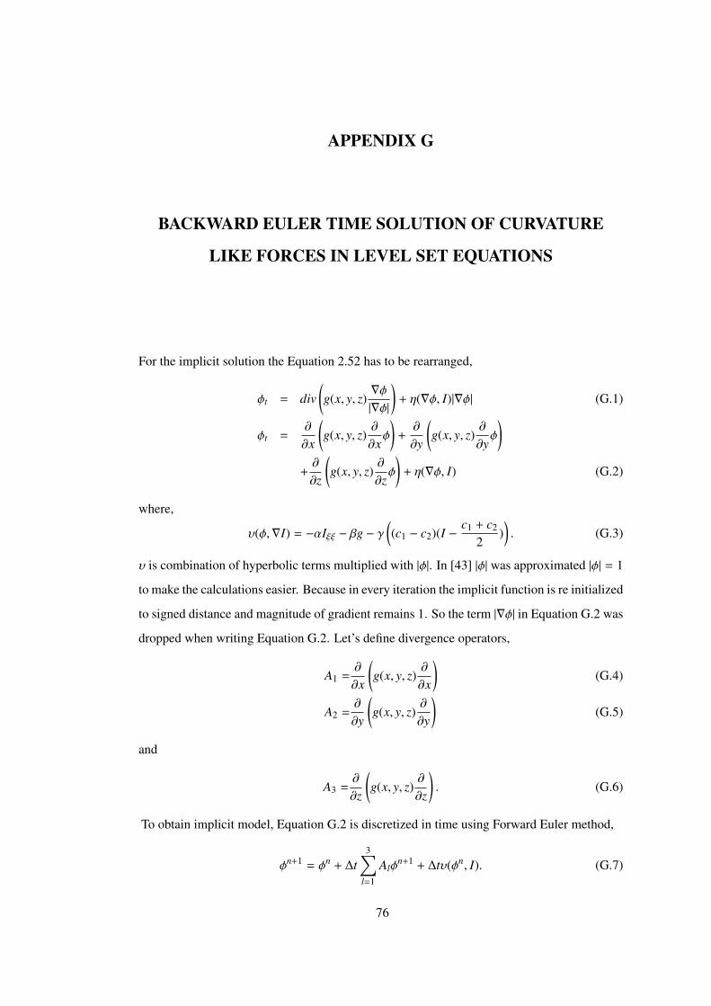
APPENDIX G

BACKWARD EULER TIME SOLUTION OF CURVATURE

LIKE FORCES IN LEVEL SET EQUATIONS

For the implicit solution the Equation 2.52 has to be rearranged,

ϕt = div(g(x, y, z)

∇ϕ|∇ϕ|

)+ η(∇ϕ, I)|∇ϕ| (G.1)

ϕt =∂

∂x

(g(x, y, z)

∂

∂xϕ

)+∂

∂y

(g(x, y, z)

∂

∂yϕ

)+∂

∂z

(g(x, y, z)

∂

∂zϕ

)+ η(∇ϕ, I) (G.2)

where,

υ(ϕ,∇I) = −αIξξ − βg − γ((c1 − c2)(I − c1 + c2

2)). (G.3)

υ is combination of hyperbolic terms multiplied with |ϕ|. In [43] |ϕ| was approximated |ϕ| = 1

to make the calculations easier. Because in every iteration the implicit function is re initialized

to signed distance and magnitude of gradient remains 1. So the term |∇ϕ| in Equation G.2 was

dropped when writing Equation G.2. Let’s define divergence operators,

A1 =∂

∂x

(g(x, y, z)

∂

∂x

)(G.4)

A2 =∂

∂y

(g(x, y, z)

∂

∂y

)(G.5)

and

A3 =∂

∂z

(g(x, y, z)

∂

∂z

). (G.6)

To obtain implicit model, Equation G.2 is discretized in time using Forward Euler method,

ϕn+1 = ϕn + ∆t3∑

l=1

Alϕn+1 + ∆tυ(ϕn, I). (G.7)

76

Figure G.1: Lexicographical ordering of an 2D matrix [44].

Here function ϕ is in vector form. And this vector is formed using lexicographical order as

shown in Figure G for 2D image. The lexicographical order changes direction according to

the operator acting. Discretization in one dimension (x) of divergence operator is [45], [19]

∂

∂x

(g(x, y, z)

∂

∂x

)≈

∑j∈N(i)

gi + g j

h2 (ϕ j − ϕi). (G.8)

N is 2 connected neighborhood of the current grid point i such as N = i + 1, i − 1. The

divergence operators are tridiagonal matrices (see Appendix B) and the elements of are given:

a(i, j) =

gi+g j

h2 j ∈ N( j)∑k∈N(k) − gi+gk

h2 j = i

0 otherwise

(G.9)

To solve matrix this system, methods like Additive operator splitting (AOS) or Locally one-

dimensional (LOD) schemes can be used. Here in this study, we followed [43] and used LOD.

Then we have this resultant equation:

ϕn+1 = (I − ∆tA1)−1(I − ∆tA2)−1(I − ∆tA3)−1(ϕn + η(∇ϕn, I)). (G.10)

The entity (I − ∆tAl) is tridiagonal and the solution of the system can be obtained using

Thomas algorithm which makes calculations efficient.

77