SEGMENTATION AND MOBILITY IN THE INDIAN LABOUR MARKETepu/acegd2018/papers/BhaskarJyotiNeog.pdf · 2...

1

SEGMENTATION AND MOBILITY IN THE INDIAN LABOUR MARKET

Bhaskar Jyoti Neog 1 Bimal Kishore Sahoo 2

ABSTRACT

The present study contributes to the limited literature on labour mobility in India using the

Indian Human Development Survey panel data for the years 2004-05 and 2011-12. We use three

different tools- transition matrices, multinomial logistic regression and wage regressions for this

study. The results show significant mobility across sectors in the economy. Mobility patterns

among workers are found to differ significantly along the lines of gender, caste, education,

wealth and family background among others. There is distress-driven movement of workers.

Significant earnings differentials exist across paid work statuses. We observe segmentation with

regard to regular vis-à-vis casual wage employment.

Keywords: Mobility; Segmentation; Informality; Distress-driven employment; Transition

Matrices.

JEL Codes: C23, C25, J31, J46, J62.

Word Count: Main text & References = 8469 words; 3 full-page tables = 1500 words; 4 half-

page tables = 1000 words. Total = 11000 words.

1 Doctoral Fellow, Dept. of Humanities & Social Sciences, IIT Kharagpur, India.

E-mail: [email protected]. Mobile: +91 8116158764 2 Assistant Professor, Dept. of Humanities & Social Sciences, IIT Kharagpur, India.

E-mail: [email protected]

mailto:[email protected]

2

1. INTRODUCTION

The extent of mobility of the workers among different segments of a labour market plays a

crucial role in improving overall levels of efficiency and growth in an economy (Paci &

Serneels, 2007). Additionally, higher labour mobility also ensures greater motivation for work,

reduced social conflicts and greater equality of opportunity (Motiram & Singh, 2012).

Theoretical conceptualisations of labour mobility have been broadly polarized into two opposing

schools of thoughts. Mainstream neo-classical labour market models assume the existence of a

single integrated labour market with free mobility of workers across sectors (Leontaridi, 1998).

On the other hand, such a view has been contested by the segmented labour market models

which emphasise restricted mobility of workers across sectors (Cain, 1976; Taubman & Wachter,

1987). The early dualists or the segmented school, model the labour market as composed of two

distinct segments- a primary sector with better jobs and a lower tier having poor working

conditions- with limited mobility across them (Leontaridi, 1998). Studies have since attempted to

conceptualise segmentation within a formal-informal framework with the formal sector acting as

the primary segment and the informal sector playing the role of the secondary segment (Fields,

2009).

Within the segmented model framework, the informal sector is considered an unfavourable

sector with poor working conditions and the informal sector workers are queuing for better jobs

in the formal sector (Hart, 1973). This contention is countered by the legalist school who

consider the labour market to be integrated and the choice of informality to be voluntary due to

3

greater flexibility afforded in the informal sector and the prohibitory regulations associated with

formality (Maloney, 1999, 2004). Later theories have further extended the model by

dichotomising the informal sector as composed of two segments- an upper tier and a lower tier

(Fields, 2009). Although the segmented labour market models initially generated much interest

among academics as well as policymakers, it subsequently lost much of its appeal in later years

due to the lack of theoretical coherency and empirical validation (Taubman & Wachter, 1987;

Wachter, Gordon, Piore, & Hall, 1974).

Empirical studies on labour market segmentation have mainly relied on the presence of

wage gaps, controlling for all available characteristics of workers as well as the examination of

the mobility patterns of the workers (Nguyen, Nordman, & Roubaud, 2013; Nordman,

Rakotomanana, & Roubaud, 2016). However, there is a lack of relevant studies in India and

South Asia in general. Although Neog & Sahoo (2015) and Narayanan (2015) examine labour

market segmentation in the country, these studies are based on the presence of earnings gaps

using cross-section data and hence do not control for time-invariant individual heterogeneity in

their model. Further, mobility analysis is not possible using such data. Khandker (1992)

examines the issue by analysing wages and mobility patterns among workers. However, the

study is restricted to a small geographical region and hence is not very representative at the

country level.

A discussion of labour market segmentation and occupational mobility is especially

pertinent in country like India given its age-old social stratifications based on caste and religion.

The country with its large labour force and widespread poverty houses a significant number of

the world’s working poor. A large section of the workforce is also employed informally under

poor working conditions (Neog & Sahoo, 2016). The country embarked on a process of

4

economic reforms more than two decades ago involving the dismantling of burdensome

regulation of the previous ‘License Raj’ regime in a number of spheres of economic activity.

Although economic reforms have been associated with high growth, there has been a concurrent

rise in inequalities over time and across space (Motiram & Sarma, 2014; Subramanian & Jayaraj,

2015). As argued by Buchinsky & Hunt (1999) and Jantti & Jenkins (2015), such rising

inequality is not much of a concern in a highly mobile labour market, as high mobility would

ensure that lifetime earnings will be much more equally distributed than inequality measured at a

point in time. Hence, there is a need to analyse mobility patterns in the country.

Most of the studies on mobility in India has been in the field of inter-generational mobility

exploring the influence of moderating variable such as caste, religion etc. in the persistence of

education, incomes and occupations across generations (Azam, 2015; Reddy, 2015). The few

studies in the intra-generational context have mostly studied the mobility of incomes or poverty

status (Ranganathan, Tripathi, & Pandey, 2017; Thorat, Vanneman, Desai, & Dubey, 2017). The

findings point towards a lack of convergence in mobility patterns and development outcomes

between major social groups. However, income as a measure of well-being has serious

drawbacks especially in rural areas (Pal & Kynch, 2000), highlighting the need to complement

studies on intra-generational income mobility with studies on occupational mobility. The

literature on intra-generational occupational mobility is very sparse in India. To the best of our

knowledge Pal & Kynch (2000) and Khandker (1992)are the only studies dealing with intra-

generational occupational mobility in India. However, their studies are based on small samples

restricted to a rural/urban context.

The study contributes to the existing literature in the following ways: -

5

Firstly, the study provides empirical evidence in the segmented vs integrated labour market

debate in the Indian economy context. Secondly, the study discusses the trends, determinants and

consequences of intra-generational occupational mobility across different labour market

segments in the Indian economy. Finally, the study explicitly discusses multiple job-holdings

among workers and relates it to existing labour market conditions.

The paper is divided into four sections. Section two presents the data and the methodology.

Section three discusses the results. Section four provides further robustness checks. Section five

provides the conclusions and dwells on some policy suggestions.

2. DATA AND METHODOLOGY

2.1. Data

The study is based on panel data from the Indian Human Development Survey (IHDS)

conducted for the years 2004-05 (IHDS-I) and 2011-12 (IHDS-II) (Desai & Reeve, 2015a,

2015b). Both IHDS-I and IHDS-II are representative at the national level. IHDS-I has a sample

size of 41554 (215754) households (individuals) out of which 83% original and split households

were resampled in IHDS-II. While the rural sample for IHDS is based on stratified random

sampling, the urban sample was drawn using a stratified sample of towns and cities within states

selected by probability proportional to population sampling.

Defining Informality: There is a lack of consensus in the literature on how to define

informality. Labour informality has been defined in a myriad of ways in the literature ranging

from definitions based on firm characteristics to ones based on job features (Fields, 2011; Neog

& Sahoo, 2016). Another definition that has been extensively used in the literature is the job-type

definition (Gong, van Soest, & Villagomez, 2004; Magnac, 1991). Piece workers or casual

6

labourers, as well as self-employed working on their own account without any paid employees

under them, are considered as informal. On the other hand, regular workers and employers are

considered as formal. Unpaid family workers are classified as informal. Although this definition

is much less stringent compared to a definition based on firm size or access to job-based social

protection, we adopt this definition due to the lack of relevant information on firm size and social

security benefits in our dataset. We argue that the evidence in favour of segmentation using a

less stringent definition of informality makes the case of segmentation even stronger when a

more stringent definition of informality (using firm-size or social security benefits) is used.

The focus of the study is on labour mobility characterised by movement of workers across

labour market statuses. We divide the labour force into eight labour market status groups: farm

workers 3, own account workers (OAWs) in non-farm business, employers in non-farm business

4, casual workers, regular workers, unpaid family workers in non-farm business, students and

‘Not in the Labour force’ categories. In the rest of the paper, casual workers are considered

synonymous with the informal wage employed whereas regular workers are considered

synonymous with the formal wage employed. Similarly, OAWs and unpaid family workers are

synonymous with informal self-employment whereas employers are synonymous with the formal

self-employed.

In defining the activity status of a worker, we consider the status where the worker has

worked the most hours out of all economic activities the person has been involved 5 6 7 8. In case

3 The farm workers segment includes workers involved in the cultivation of crops as well as those involved in

animal care. 4 In order to distinguish OAWs from employers we use information on the cost of paid labour services for a

business. Owners of businesses with positive labour cost are considered as employers whereas those without any

labour cost are considered as OAWs. 5 In the IHDS data, respondents were asked about information on multiple wage jobs held by the worker over the

survey period. Our study uses information only for the major job -defined as the job where the worker has worked

the maximum hours out of all the jobs.

7

the person does not work at all in any economic activity, he/she is considered to be outside the

workforce. A person from outside the work-force who is currently enrolled in an educational

institution is considered to be a student. Persons from outside the work-force who are not

students comprise the ‘Unemployed and Not in the Labour Force’ (UNLF) category. In case of

self-employed persons, there may be multiple household members engaged in a non-farm

business. In such a scenario, we follow Deshpande & Sharma (2016) and classify the person who

has worked the maximum number of hours within the household as the primary decision maker

of the business 9 (i.e. the OAW or employer) and all other household workers as unpaid family

workers. However, all household members engaged in farm work are classified as farm workers

without any distinction of primary decision maker in the farm business.

2.2. Methodology

Existing attempts in the literature to check for labour market segmentation have mainly

relied on the presence of wage gaps, controlling for all available characteristics of workers.

However, this approach has been criticized for its inability to control for all the productive

characteristics of workers (Rosenzweig, 1988). Further, a significant monetary wage gap across

sectors may simply indicate compensatory wage differentials for differences in non-pecuniary

rewards to jobs as workers seek to equalise utility across sectors (Maloney, 1999).

6 IHDS asks respondents about information on a maximum of three non-farm businesses in a household. Our study

conducts its analysis using only the business with the highest net earnings among the three. 7 There are a small number of cases where total hours worked are equal for two or more economic activities. In such

cases, we consider information on net income earned from the economic activities and classify the worker to the

activity where net earnings are higher. 8 Information on hours of work was not available for persons involved in animal care. However, IHDS provides

information on whether the person is involved in animal care. As such, we use the hours of work criteria to classify

workers as farm workers, wage employees or self-employed. In case the person is not involved in any of the above

activities but is engaged in animal care, we consider him to be involved in animal care and merge him into the ‘farm

worker’ category. 9 There are a small number of cases, where total hours worked are similar for two or more workers. In such cases,

we use information on age of the worker and identify the more aged worker as the primary decision maker.

8

Given the criticisms of the wage analysis approach, other studies have relied on the

evaluation of the transition of workers across sectors over time as a method to test the segmented

labour market theory. Some studies have applied both mobility analysis and wage regressions to

get a more robust and comprehensive picture (Duryea, Márquez, Pagés, & Scarpetta, 2006;

Pagés & Stampini, 2009).

Following the empirical literature, the study relies on a three tools to understand the patterns

of mobility across sectors and how such mobility is associated with individual characteristics and

earnings. Firstly, the study examines the transition probabilities of workers moving across

sectors using transition matrices. The study then looks at the characteristics of the movers with

reference to stayers using multinomial logistic regression. Finally, the study looks at the

consequences of mobility on earnings with reference to the stayers using fixed effects regression

analysis.

2.2.1. Transition Probabilities

We first examine the transition probabilities for workers across sectors given by the

probability of moving to sector 𝑗 in period 𝑡 given that the person was in sector 𝑖 in period 𝑡 − 1.

The transition probabilities are displayed in the form of matrix ‘P’. Formally the elements of the

P matrix are given by:

𝑝𝑖𝑗 = 𝑃(𝑆𝑡 = 𝑗 𝑆𝑡−1 = 𝑖) =𝑃(𝑆𝑡−1 = 𝑖 ⋂ 𝑆𝑡 = 𝑗)

𝑃(𝑆𝑡−1 = 𝑖)………(1)

The diagonal elements of the P matrix, 𝑝𝑖𝑖 give us the share of members of a sector who have

not moved over the period. Similarly, (1 − 𝑝𝑖𝑖) gives us the turnover rate of the sector. However,

we are unable of distinguish permanent movers to transitory movers who move to-and-fro

9

between sectors. Further, the transition probabilities from the P matrix are still imperfect

measures of mobility as they depend on the size of the initial and terminal statuses and also on

the job openings in each of them. Hence, we standardize the P matrix further which gives us the

V and the T matrices.

Following (Maloney, 1999), the general element of the V matrix is given by:

𝑣𝑖𝑗 =𝑝𝑖𝑗 𝑝.𝑗⁄

(1 − 𝑝𝑖𝑖)(1 − 𝑝𝑗𝑗)………(2)

Here, 𝑝.𝑗 would indicate the share of the terminal sector, 𝑗 in the population. 𝑣𝑖𝑗 would

measure the disposition for a worker to move from sector 𝑖 to sector 𝑗. A segmented labour

market would give us a high 𝑣 for a movement from informal to formal but a low 𝑣 in the

reverse direction.

Similarly, the general element of a T matrix is given by:

𝑡𝑖𝑗 =𝑁𝑖𝑗 (𝑁𝑖. − 𝑁𝑖𝑖)⁄

(𝑁.𝑗 − 𝑁𝑗𝑗) ∑ (𝑁.𝑘 − 𝑁𝑘𝑘)𝑘≠𝑖⁄………(3)

Here, 𝑁𝑖𝑗 is the number of individuals moving from sector 𝑖 to 𝑗; 𝑁𝑖. is the initial size of

sector 𝑖; 𝑁.𝑗 is the final size of sector 𝑗. The numerator of 𝑡𝑖𝑗 is the probability of joining 𝑗,

conditional on having left 𝑖. The denominator is the probability of joining 𝑗 for a mover from 𝑖

when sector assignment is random. 𝑡𝑖𝑗 gives us the tendency for a worker to move from 𝑖 to 𝑗,

with values above (below) one indicating a positive (negative) tendency to make the transition.

In an integrated labour market where all transitions are random, all 𝑡𝑖𝑗′𝑠 are equal to unity and

the T matrix is equivalent to an Identity matrix (Bernabe & Stampini, 2009). Since the V and the

10

T matrices are associated with net flows, no index of mobility can be built for stayers and the

diagonal elements are empty.

The information from the P, V and the T matrices can provide us with a rough picture of the

extent of labour mobility across different sectors besides enabling us to draw a preliminary

assessment of the presence of segmentation in the labour market.

2.2.2. Determinants of Mobility

After the study of the transition probabilities, we look at the characteristics of the individuals

who move from one sector to another vis-à-vis the stayers. If labour mobility is associated with

certain worker characteristics, this would strengthen our inference on segmentation and would

give us an idea of the factors excluding workers from the desirable statuses. The theoretical

framework for our model of worker transition is an extension of the rational agent model of

occupational choice (Boskin, 1974). The model of occupational choice states that a rational

worker would choose the sector which gives him the maximum possible utility from all available

sectors. Thus the individual chooses sector 𝑖 in period 𝑡 if 𝑈𝑖,𝑡 > 𝑈𝑘,𝑡, where 𝑘 = 1, 2, …… ,𝐾

indexes the sectoral choices available to the individual. Accordingly, a worker would transit

from sector 𝑖 to 𝑗 if there is a change in the utilities associated with the sectors so that sector 𝑗

becomes the utility maximizing sector in the terminal period. That is, a worker would move from

sector 𝑖 in period 𝑡 to sector 𝑗 in period (𝑡 + 1) if 𝑈𝑖,𝑡 > 𝑈𝑘,𝑡 and 𝑈𝑗,𝑡+1 > 𝑈𝑘,𝑡+1.

The utility from an occupational choice depends on a number of factors including expected

lifetime earnings, risks and constraints anticipated in getting the job etc. (Rees & Shah, 1986;

Uusitalo, 2001). The utility function is given below:

𝑈 = 𝑓(𝐼, 𝐴, 𝐹, 𝑅, 𝐸)………(4)

11

𝐼 = 𝑔[𝑤, 𝑝(𝑋)] = 𝑤 × 𝑝(𝑋)………(5)

where I denoting expected lifetime earnings is the product of two terms- the sum of the

discounted stream of earnings from the job over the lifetime (w) and the probability of getting the

job (p(X)). 𝐼 is positively related with w and p(X). Finally, p(X) is inversely related to the

constraints involved in getting the job (X). Our framework is similar to the classic Harris-Todaro

approach where constraints set by the limited availability of formal jobs in the urban sector

lowers expected wages in the urban sector (Harris & Todaro, 1970). Similarly, A denotes

expected autonomy in the job; F denotes expected flexibility afforded by the job; R is the risks

involved in the job; E is the expected effort required in the job.

It is noteworthy that we extend Boskin (1974)’s framework so that occupational choice

depends not only on factors such as expected lifetime earnings, autonomy and flexibility from

the job but also on the constraints anticipated in the job. Such a framework enables us to study

occupational choice by a rational agent given the possibility of a segmented labour market. The

constraints that an individual may face in getting a job may be due to his human capital levels,

credit availability, caste, religion etc. and/or due to supply-side factors such as the availability of

adequate, decent formal jobs.

Since information on the given job attributes are not available to us we proxy them using

individual-level worker characteristics for the initial period as suggested in Rees & Shah (1986).

We used multinomial logistic regression to analyse the impact of worker attributes on worker

transitions. Since there are very few number of transitions from the ‘Student’ group to some

sectors; we merge the Student and the UNLF group to form the Students, Unemployed and Not

in the Labour Force (SUNLF) category giving us a total of seven labour market status. Following

(Wooldridge, 2010), the multinomial logit model can be formulated as:

12

𝑃(𝑆𝑡−1 = 𝑖 ⋂ 𝑆𝑡 = 𝑗)

𝑃(𝑆𝑡−1 = 𝑖 ⋂ 𝑆𝑡 = 𝑖)= 𝑋𝛽, 𝑓𝑜𝑟 𝑖, 𝑗 = 1,2, … . ,7………(6)

Here, 𝑆𝑡−1 and 𝑆𝑡 denote the employment status of the individual in period 𝑡 − 1 and 𝑡

respectively. We will have seven such models, one for each initial sector 𝑖. Additionally, 𝑋 is a

vector of factor affecting labour mobility whose values are considered at the initial time period

i.e. 2004-05 and 𝛽 is the vector of the corresponding regression coefficients. The vector 𝑋

comprises the set of the standard individual level worker characteristics including age, gender 10,

education, household wealth, social capital (proxied by membership in various

groups/organizations), marital status, dependency ratio, rural-urban residence, caste, dummy for

fluency in English, religious affiliation as well as the education and occupation of the

father/husband’s father of the household head 11 12. Finally, we attempt to control macro-level

factors through the inclusion of 18 state dummies.

Although the multinomial logistic regression results can give us an idea of the characteristics

of mobility, it tells us nothing about the determinants of the stayers. Hence, we complement the

multinomial logistic analysis with a binomial logistic model to analyse the determinants of the

probability of survival in a labour market status. The explanatory variables in the model are

identical to those used in the multinomial logistic model.

10 There are some minor issues of mismatch in age and gender of a person across years. IHDS documentation

suggests that in the event of a mismatch, information from IHDS-II should be given the priority. Accordingly, we

update the information in IHDS-I (2004-05) on gender and age using information from IHDS-II (2011-12). 11 In the absence of any variable depicting wealth of the parent of the household head we follow Fairlie (1999) and

proxy it by the education of the father/husband’s father of the household head. Similarly, following Hout & Rosen

(2000) the labour market status of the father/husband of the household head is proxied by his/her occupational

category. 12 We divide the occupational codes of the father/husband of the household head into four groups: Professional &

Executive workers; Sales-related workers; Farmers, Loggers & Fisherman; and finally, Clerical, Sales & Production

workers. Our occupational classification is done so as to correspond with the employment status groups. Hence, the

‘Sales workers’ group relates closely with the self-employment group; ‘Farmers, Loggers & Fisherman’ group

corresponds with the farm workers; and the ‘Professional & Executive workers’ as well as the ‘Clerical, Sales and

Production workers’ group closely resemble the wage workers.

13

The preceding analysis is based on the assumption of a homogeneous sample of workers,

conditional on observable worker characteristics. If, however, workers are heterogeneous in

unobservable ways and choose the sector that maximises their welfare, they will want to remain

in their preferred sector even if displaced by exogenous shocks (Pagés & Stampini, 2009). Thus

mobility may be zero even in an integrated labour market. Thus we complement our mobility

analysis with the study of earnings differentials.

2.2.3. Mobility and earnings

Our final section looks at the impact of labour mobility on the earnings and poverty levels of

the workers 13. To do so, we conduct fixed-effects linear regression on earnings data controlling

for a number of individual and job level characteristics as well as accounting for unobserved

time-invariant worker heterogeneity. Since, we have earnings data on four non-farm sectors (viz.

Own-Account workers, Employers, Casual workers and Regular workers) we only consider these

four groups for our regression analysis. Including a sub-sample of observation in the earnings

function may generate inconsistent results due to possible selection bias. Assuming that selection

bias is not due to time-varying unobserved factors, fixed-effects corrects for such bias 14 (Fortin,

Lemieux, & Firpo, 2011). Further, proper identification in fixed-effects regression relies on a

sufficient number of movers across the labour market sectors (Nordman et al., 2016). We verify

that this, actually, is the case as seen from Table 2.

Our fixed effects model is given by:

𝑦𝑖𝑡 = 𝛼𝑖 + 𝑥𝑖𝑡′ 𝛽 + 𝛾𝑂𝐴𝑊𝑖𝑡 + 𝛿𝐸𝑖𝑡 + 𝜂𝐶𝑊𝑖𝑡 + 휀𝑖𝑡………(7)

13 Earnings for OAWs and employers are obtained by deducting from gross business earnings, costs incurred in

running the business. Wage earnings includes cash wages as well as income earned as bonus from the job. Earnings

of the worker is then divided by hours worked in that activity to arrive at the hourly earnings figures. 14 Attrition bias can be considered as a special case of sample selection bias and as such our results are robust to

possible attrition bias under the given assumptions (Verbeek & Nijman, 2008).

14

Here, 𝑖 indexes individuals and 𝑡 indexes time. Further, 𝑦𝑖𝑡 is the net hourly earnings of the

worker; 𝛼𝑖 is the time-invariant individual fixed effect; 𝑂𝐴𝑊𝑖𝑡, 𝐸𝑖𝑡 and 𝐶𝑊𝑖𝑡 are dummy

variables taking the value one if the worker is an Own Account worker, employer and casual

worker respectively and zero otherwise; and 휀𝑖𝑡 is the i.i.d. error term such that 𝐸(휀 𝑥,

𝛼, 𝑂𝐴𝑊,𝐸, 𝐶𝑊) = 0. We exclude the dummy for regular workers from our model and interpret

our results considering it as the reference category. The estimated coefficient for 𝑂𝐴𝑊 (i.e. 𝛾)

can thus be interpreted as the earnings penalty/premium for those moving from regular work to

OAW. �̂� and 𝛿 can similarly be interpreted. We re-run our model changing our reference

category in order to get a picture of the sectoral earnings gap with reference to the other labour

market states. Finally, 𝑥𝑖𝑡′ is a vector of individual attributes which includes the standard

variables such as age, years of education, education of the father of household head, dummy for

urban residence as well as dummies for household headship and being married. Additional

control variables include dummies for computer and English usage, occupational and industry

dummies.

Earnings differentials are important as they provide a useful measure of the monetary

differentials other job attributes needs to compensate for even if they are an inadequate measure

of utility differential (Pagés & Stampini, 2009). However, there is a need to be cautious while

comparing the earnings differentials between the wage employed and the self-employed since the

earnings for the latter may include capital returns (Pagés & Stampini, 2009). Earnings for the

self-employed may also be inflated as many businesses in our study are family-based, and their

earnings may include the remuneration for unpaid family workers.

3. RESULTS AND DISCUSSION

3.1. Descriptive Statistics

15

We discuss below the characteristics of the workers engaged in the different employment

sectors.

[Insert Table 1]

Table 1 shows that farm workers as a group have the largest share in the workforce,

closely followed by casual workers. Employment sectors such as employers and regular worker

are concentrated in urban areas relative to other groups. The age composition of the workforce

shows unpaid workers, students and the UNLF categories are significantly younger than the

other groups. OAWs, employers and regular workers have the most aged workforce in the

sample (Table 1). The gender composition of the employment groups shows OAWs, employers,

regular workers and casual worker being considerably male-dominated with the females mostly

concentrated in the UNLF and farm groups.

The education profile of the workers over both the periods show regular workers and

employers doing significantly better, followed by the OAWs and Unpaid family workers with the

rest having the poorest educational outcomes (Table 1). Our results dispel the notion of self-

employed having a significantly lower education than their wage employed peers (Robinson &

Sexton, 1994). The caste composition shows General and OBC category workers have higher

representation in better employment outcomes such as employers and regular work whereas

SC/ST groups are involved mostly in casual work. Similarly, we find large variation in the

distribution of workers by religion and marital status.

Finally, judging in terms of incomes and assets we find employers and regular workers

doing significantly better followed by OAWs and unpaid family workers with the casual workers

doing the worst in this regard (Table 1). In line with the literature, we also find variability in

16

earnings to be much higher among the self-employed relative to the wage employed (Åstebro &

Chen, 2014). Consistent with the international literature we also find work hours to be quite high

among the self-employed (Blanchflower, 2004) as well as regular workers whereas they are

found to be lower among the casual workers.

An interesting feature of the Indian labour market is the large share of workers who are

involved in more than one job. Additional Table A1 shows that more than 10 percent of the

workers in the workforce is involved in more than one job and this number has increased over

the period. Further, we find that a majority of such multiple job holders are involved in farm and

wage work. Multiple job holding is seen to be more common among casual workers and OAW

and quite rare for farm and regular workers (Additional Table A1). This issue is discussed further

in the next few sections.

3.2. Transition Matrices

We now look at the transition matrices of the workers across the various employment groups.

[Insert Table 2, 3 and 4]

A first look at the diagonal elements of the P-matrix shows labour turnover to be very

high for the self-employed groups whereas it is very low for the wage employed and farm

workers (Table 2). We also find high two-way mobility between farm work and casual work

which may signify the seasonal nature of agricultural work as workers move intermittently

between agriculture and casual work to eke out a living. We look at this issue further in the next

section. Considerable two-way mobility is also noticeable among the wage employment groups

(between casual and regular workers) and the self-employment groups (among OAWs,

employers and unpaid family workers) (Table 2). Finally, the significant movement of people

17

from outside the workforce (composed of students and UNLF) into farm work and casual work

groups signify the role that these groups serve as points of entry for new entrants into the

workforce (Table 2). Such a phenomenon may imply that workers move into such sectors to gain

work experience (either voluntarily or due to the limited supply of formal (or regular) job

opportunities) before moving into better-paying activities.

Looking at the T matrices shows that most of the t indices are near unity signifying

random worker transition (Table 4). The indices from the V matrix also indicate in most cases a

high level of symmetry among the various sectoral flows consistent to the integrated labour

market view (Table 3). However, in certain cases, we also notice a high tendency of workers to

move between the self-employed categories of employer, OAW and unpaid family work (Table

4). The v indices in such cases are not very symmetric especially with reference to movements

associated with unpaid family work (Table 3). A high tendency of mobility for workers is also

noticeable among casual and regular work categories with the v indices being asymmetric (Table

3 and 4). Such cases indicate the possibility of segmentation in the labour market, especially in

the wage employment section.

3.3.Mobility and individual characteristics

Although the analysis of mobility until this point has provided us with a good idea of the

extent of movement of workers across different employment groups, it doesn’t tell us anything

about the characteristics of workers making a move to other job categories. Hence, we use the

multinomial logistic regression results to get a better idea of the different attributes of workers

associated with mobility. We complement the discussion of the results from the multinomial

logistic regression with the logistic regression results illustrating the characteristics of the

stayers.

18

Given the large movements of workers from farm work to casual work, we first look at

the characteristics of such movers (Table 2). We find that with reference to staying in farm work,

movements into casual work is mainly undertaken by the young, the less educated, males, the

poor and the backward castes (Table 5). Given the relatively high poverty rates for such movers

before and after moving (as seen from Additional Table A4) and the attributes of the workers

moving from the former to the later, movements out of agriculture is likely to be of a distress-

driven nature undertaken mainly by workers to supplement their meagre family incomes.

Looking at the issue further, we find that most of the movers from farm to casual work

hold multiple jobs, simultaneously working in farm and casual work in both the periods. At the

same time, the number of such multiple job holders have almost tripled over the period

(Additional Table A7). Further, most of such movement from farm to casual work is not into

Mahatma Gandhi National Rural Employment Guarantee Act (MGNREGA) work but private

casual work indicating that such work is not due to the lure of relatively better MGNREGA work

15. This fact together with our earlier findings of high poverty rates among movers from farm

work to casual work may indicate declining productivity in agriculture as people move into

casual work alongside farming activities to supplement meagre agricultural incomes.

Interestingly, around 17 per cent of the workers undertake the opposite movement from

casual to farm work. Such movers are generally better-off in terms of education, caste-affiliation

and assets (Table 6). Incidence of multiple job-holding also falls dramatically among such

movers (Table A7). Such differences in the characteristics of the movers from farm to casual

work, and vice versa, offers some argument against the possibility that movements between farm

15 We do not present the results in regard to this contention. Results are available upon request.

19

and casual work is random and that the movement from the former to the later represents genuine

symptoms of distress among the farmers.

The findings tally with those in the literature which finds evidence of declining

profitability as well as rising risks and indebtedness in Indian agriculture notwithstanding the

silver lining of rising agricultural productivity in recent years (Deokar & Shetty, 2014; Mishra &

Reddy, 2010). Our findings are also in line with the global trend of rising diversification of farm-

based households into non-farm activities (Davis et al., 2010; J. Lanjouw & Lanjouw, 2001). Our

results are also similar to Lanjouw & Shariff (2004) who find that much of the diversification

into non-farm work by the poor is into casual work.

Given the high t indices between OAW and employers, we take a look at the attributes of

movers into employer jobs. We see that relative to staying in OAW, moving into employer

category is mainly undertaken by the young, those with better educational background and the

wealthy (Table 5). This may be an indication of the presence of liquidity constraints in the

economy as small well to do businesses with enough financial capital undertake investments to

enlarge their business (Table 5). This contention is further corroborated by the very low initial

poverty rates among the OAWs undertaking the move into employer category (Additional Table

A4).

[Insert Table 5]

We also notice high mobility of workers from casual work into regular work. We see that

movers from casual to regular work have better endowments in terms of higher education,

fluency in English as well as being more likely to be rich; from urban areas and privileged castes

and religions (Table 6). The scenario of low turnover for regular workers, the high tendency for

20

casual workers to move into regular work and the superior characteristics of such movers, points

to a situation where casual workers queue for scarce well-paying regular jobs, and it is mainly

the better endowed of the casual workers who get to move into regular work. Consistent with this

view, we find that the reverse movements of workers from regular into casual work is mainly

associated with the less educated and the poor (Table 6). Looking at the persistence in casual or

regular work, we find that, consistent with our earlier conjecture, education, fluency in English

and household wealth are positively associated with survival in regular work but negatively

related with survival in casual work (Additional Table A5).

We conclude the section with a few general remarks: -

Firstly, our results in general show a consistent pattern wherein the occupational status of

the father/husband of the household head has a significant influence on the mobility patterns of

the workers (Table 5, 6; Additional Table A2, A3, A5). In general, workers within a family tend

to move into or persist in the employment status related to the occupation of the father/husband

of the household head. Hence, workers whose father/husband of the household head were in

sales-related occupations are more likely to move into (or persist in) self-employment work

(Table 5, 6; Additional Table A3, A5). Similar results are evident for the farm work and wage

work group. The results corroborate the literature on the impact of parental occupations on self-

employment entry and survival (Parker, 2009; Simoes, Crespo, & Moreira, 2016). The results

also support the literature on limited intergenerational occupational mobility in India (Reddy,

2015).

Secondly, the mobility patterns display a definite gender pattern with males more likely

to move into (or persist in) paid work categories such as OAW, Employer, casual and regular

work whereas females are more likely to move into (or persist in) unpaid family work or outside

21

the workforce (Table 5, 6 and Additional Table A2, A3). This is consistent with the literature

which finds high mobility within the workforce for men and high mobility into joblessness for

women (Royalty, 1998; Theodossiou & Zangelidis, 2009). Thirdly, we fail to find any general

impact of social capital proxied by membership in socio-political institutions on labour market

mobility (Table 5, 6 and Additional Table A2, A3). Fourthly, we also find that in line with the

findings in the literature, SCs/STs are more likely to be exiting self-employment and less likely

to be entering and surviving in self-employment (Table 6 and Additional A.5) (Ahn, 2011;

Fairlie, 1999). Lastly, education is found to positively impact mobility and survival in the more

favourable outcomes such as employer and regular work (Table 5, 6 and Additional Table A2,

A3, A5).

[Insert Table 6]

3.4. Mobility and Earnings

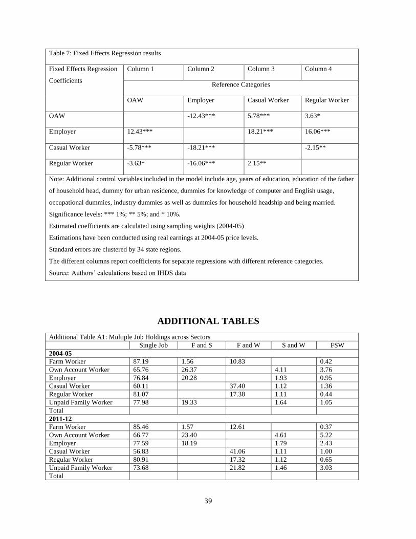
We finally a look at the impact of labour mobility on individual earnings. Taking a look at

Additional Table A3 and A6, we find that movements into statuses such as OAW, employer and

regular work from other sectors such as farm and casual work are associated with positive

changes in household consumption levels as well as wage levels. The aggregate statistics on

consumption and wage changes associated with worker mobility, however, do not control for

individual-level attributes. To look at the impact of worker mobility on earnings controlling for

observable and time-invariant unobservable worker attributes, we look at the results of the fixed

effects regression analysis.

As can be seen from Table 7, earnings are significantly higher in the employer group as

compared to all other sectors. The finding that employers earn significantly more than OAWs

22

along with our earlier observation about the attributes of the movers from OAW into employer

category offer further support to our earlier inference on employer category being the more

desired employment status. Our findings are also similar to those found in Vietnam and

Madagascar (Nguyen et al., 2013; Nordman et al., 2016). Similarly, casual workers fare the

worst in terms of wages in comparison to all other segments. OAWs and regular workers are

positioned in between the extreme cases of casual work and employers (Table 7).

We see that regular workers earn significantly better than their casual worker counterparts

(Table 7: Column 4). This result in combination with our earlier evidence on a lower turnover in

regular work as well as the superior attributes of the workers moving from casual to regular work

provides ample evidence in favour of the segmented labour market view at least within a formal

(or regular) vs informal (or casual) wage employment framework. Our findings are synonymous

with the literature on Latin America, Vietnam and Madagascar and South Africa which finds

overwhelming evidence of a formal wage premium over informal sector wage workers (Duryea

et al., 2006; Nguyen et al., 2013; Nordman et al., 2016; Pagés & Stampini, 2009).

[Insert Table 7]

4. ROBUSTNESS CHECKS

The authors conclude the discussion with a few robustness checks:

Firstly, we consider the issue of possible endogeneity in our earnings regression model.

Specifically, proper identification of the regression coefficients relies on the fact that movers do

not change their employment states systematically for better earnings, i.e. transition is random.

We follow Nordman et al., (2016) and check whether mobility is systematically associated with

earnings increase (or decrease) relative to the stayers. Out of the 12 cases, where workers change

23

employment status, earnings increase with regard to the stayers in five cases whereas we find

earnings decreasing compared to the stayers in six cases (Additional Table A6). This provides

some argument against the endogeneity concerns in the earnings function.

Secondly, it might be argued that the multinomial logistic regression results as well as the

results from the transition matrices are biased due to non-random attrition of individuals from the

sample. We accordingly model the attrition process and attempt to correct for any attrition bias

under the assumption of selection on observables (Wooldridge, 2010). Following Wooldridge,

(2010), let 𝑦 be the dependent variable or outcome of interest and 𝑋 be the vector of independent

variables as discussed earlier. We define 𝐴 to be the attrition dummy equal to 1 if 𝑦 is non-

missing in both the periods and 0 otherwise. Additionally, 𝑍 is a vector of auxiliary variables

affecting the probability of attrition such that,

𝑃(𝐴 = 1 𝑦, 𝑋, 𝑍) = 𝑃(𝐴 = 1 𝑍)…………(8)

Assumption (1) is referred to in the econometrics literature as ‘selection on observables’

(Wooldridge, 2010). Under the assumption of ‘selection on observables’, possible bias due to

non-random attrition can be corrected through the Inverse Probability Weighting (IPW)

estimation. IPW estimation relies on the presence of variables in 𝑍 which are good predictors of

attrition. We include in 𝑍 variables such as dummies for relationship with the household head as

well as the person identifier 16. Additionally, Fitzgerald, Gottschalk, & Moffitt, (1998), suggests

that 𝑍 should also include lagged values of the dependent variable. Hence, we also include in 𝑍,

dummies for employment status in the initial period. All the above variables are found to have a

significant influence on 𝐴.

16 Person identifier are numbers assigned to the family member by the interviewer. We posit that persons

interviewed first have a lesser probability of attrition than others.

24

Under IPW estimation, we estimate a probit model of 𝐴 on 𝑋 and 𝑍 and generate the fitted

probabilities 𝑝. In the second step, the outcome model is weighted by the inverse of 𝑝 i.e. 1/𝑝 to

give us our attrition-bias corrected estimates. Accordingly, we estimate our multinomial logistic

regression model as well as the transition matrices after correcting for possible attrition bias and

compare our results with the uncorrected models. Our results are effectively similar and our

conclusions remain the same under the attrition corrected case. We do not present the results for

The attrition-adjusted results are not presented here. Results are available upon request.

Finally, the analysis of our study is conducted considering all members of the household

irrespective of age. In developing countries like India, defining a working age group is difficult

as largescale poverty and informality means that a significant section of the population outside

the conventionally defined age groups are engaged in economic activities. As such, restricting

our sample to a particular working age group may lead to bias emanating from arbitrary selection

of cut-offs for the working age group. However, we check for the robustness of our results by

experimenting with different working age group samples and find the results are similar across

the different specifications. Results for the alternative specifications of working age groups are

not shown but are available upon request.

5. CONCLUSION

The present study contributes to the limited literature on the patterns and consequences of

labour mobility in the India. In doing so its provides robust empirical evidence on the segmented

labour market theory. Our study finds significant mobility across sectors in the economy.

Characteristics such as gender, caste, education, marital status, wealth as well as the occupation

of the father/husband’s father of the household head are found to influence mobility

significantly. Further, our study finds evidence of significant earnings differentials across paid

25

work statuses. The study finds evidence of segmentation with regard to regular (or formal) vis-à-

vis casual (or informal) wage employment. We also notice large-scale distress driven movements

of workers, especially from OAW and farm work into casual work.

Given the distress-driven nature of movement from OAW and farm work into casual work,

policy measures need to be taken to identify and alleviate the nature of the problems in such

activities. Further, adequate measures need to be taken to improve the growth prospects of the

small business enabling them to enlarge and generate decent employment. In this regard, policy

efforts need to be made especially towards alleviating capital constraints in small business given

the important role of capital availability in facilitating business growth. Furthermore, given the

gender-specific patterns of job mobility, policy measures need to be undertaken to improve the

workforce participation of females and their mobility into paid work statuses. Finally, policy

efforts should be directed to improve the self-employment prospects among the SC/STs.

REFERENCES

Ahn, T. (2011). Racial differences in self-employment exits. Small Business Economics, 36(2),

169–186. https://doi.org/10.1007/s11187-009-9209-3

Åstebro, T., & Chen, J. (2014). The entrepreneurial earnings puzzle: Mismeasurement or real?

Journal of Business Venturing, 29(1), 88–105.

https://doi.org/10.1016/j.jbusvent.2013.04.003

Azam, M. (2015). Intergenerational Occupational Mobility among Men in India. Journal of

Development Studies, 51(10), 1389–1408. https://doi.org/10.1080/00220388.2015.1036040

Bernabe, S., & Stampini, M. (2009). Labour mobility during transition. Economics of Transition,

17(2), 377–409. https://doi.org/10.1111/j.1468-0351.2009.00345.x

26

Blanchflower, D. (2004). Self-Employment: More may not be better. Swedish Economic Policy

Review, 11, 15–73. https://doi.org/10.3386/w10286

Boskin, M. J. (1974). A Conditional Logit Model of Occupational Choice. Journal of Political

Econoomy, 82(2), 389–398. Retrieved from http://www.jstor.org/stable/1831185

Buchinsky, M., & Hunt, J. (1999). Wage Mobility in the United States. The Review of Economics

and Statistics, 81(3), 351–368.

Cain, G. C. (1976). The challenge of segmented labor market theories to orthodox theory: A

survey. Journal of Economic Literature, 14(4), 1215–1257. https://doi.org/10.2307/2722547

Davis, B., Winters, P., Carletto, G., Covarrubias, K., Quiñones, E. J., Zezza, A., … DiGiuseppe,

S. (2010). A Cross-Country Comparison of Rural Income Generating Activities. World

Development, 38(1), 48–63. https://doi.org/10.1016/j.worlddev.2009.01.003

Deokar, B. K., & Shetty, S. L. (2014). Growth in Indian Agriculture. Economic and Political

Weekly, XLIX(26&27), 101–105.

Desai, S., & Reeve, V. (2015a). Indian Human Development Survey, 2005. Ann Arbor, MI,

USA: Inter-university Consortium for Political and Social Research.

https://doi.org/10.3886/ICPSR22626.v8

Desai, S., & Reeve, V. (2015b). Indian Human Development Survey, 2011-12. Ann Arbor, MI,

USA: Inter-university Consortium for Political and Social Research.

https://doi.org/10.3886/ICPSR36151.v2

Deshpande, A., & Sharma, S. (2016). Disadvantage and discrimination in self-employment: caste

gaps in earnings in Indian small businesses. Small Business Economics, 46(2), 325–346.

27

https://doi.org/10.1007/s11187-015-9687-4

Douglass, M. E. (1976). Relating Education to Entrepreneurial Success. Business Horizons,

19(6), 40–44. https://doi.org/10.1109/EMR.1985.4306138

Duryea, S., Márquez, G., Pagés, C., & Scarpetta, S. (2006). For Better or for Worse? Job and

Earnings Mobility in Nine Middle- and Low-Income Countries. Brookings Trade Forum,

(1), 187–203. https://doi.org/10.1353/btf.2007.0002

Fairlie, R. W. (1999). The Absence of the African- American Owned Business: An Analysis of

the Dynamics of Self-Employment. Journal of Labor Economics, 17(1), 80–108.

Fields, G. S. (2009). Segmented Labor Market Models in Developing Countries. In The Oxford

Handbook of Philosophy of Economics (pp. 476–510). New York: Oxford University Press.

Fields, G. S. (2011). Informality: Its time to stop being Alice-in-Wonderland-ish. Retrieved from

http://wiego.org/sites/wiego.org/files/publications/files/Fields_IE.Alice_.in_.Wonderland.pd

f

Fitzgerald, J., Gottschalk, P., & Moffitt, R. (1998). An Analysis of Sample Attrition in Panel

Data : The Michigan Panel Study of Income Dynamics. The Journal of Human Resources,

33(2), 251–299.

Fortin, N., Lemieux, T., & Firpo, S. (2011). Decomposition methods in economics. In Handbook

of Labour Economics Vol. 4 (pp. 1–102). Amsterdam, The Netherlands: North Holland.

Gong, X., van Soest, A., & Villagomez, E. (2004). Mobility in the Urban Labor Market: A Panel

Data Analysis for Mexico. Economic Development and Cultural Change, 53(1), 1–36.

https://doi.org/10.1086/423251

28

Harris, J. R., & Todaro, M. P. (1970). Migration, Unemployment and Developmnent : A Two-

Sector Analysis. American Economic Review, 60(1), 126–142.

Hart, K. (1973). Informal Income Opportunities and Urban Employment in Ghana. The Journal

of Modern African Studies, 11(1), 61–89.

Hout, M., & Rosen, H. (2000). Self-Employment , Family Background , and Race. The Journal

of Human Resources, 35(4), 670–692.

Jantti, M., & Jenkins, S. P. (2015). Income Mobility. In A. Atkinson & F. Bourguignon (Eds.),

Handbook of Income Distribution (2A ed., pp. 808–924). Amsterdam, The Netherlands:

Elsevier.

Khandker, S. R. (1992). Earnings, Occupational Choice, and Mobility in Segmented Labor

Markets of India (World Bank Discussion Papers No. 154). Washington D.C., USA.

Lanjouw, J., & Lanjouw, P. (2001). The rural non-farm sector: issues and evidence from

developing countries. Agricultural Economics, 26, 1–23. Retrieved from

http://onlinelibrary.wiley.com/doi/10.1111/j.1574-0862.2001.tb00051.x/abstract

Lanjouw, P., & Shariff, A. (2004). Rural Non-Farm Employment in India: Access, Incomes and

Poverty Impact. Economic and Political Weekly, 39(40), 4429–4446.

Leontaridi, M. R. (1998). Segmented Labour Markets : Theory and Evidence. Journal of

Economic Surveys, 12(1), 63–101. https://doi.org/10.1111/1467-6419.00048

Magnac, T. (1991). Segmented or Competitive Labor Markets. Econometrica, 59(1), 165–187.

Maloney, W. F. (1999). Does informality imply segmentation in urban labor markets? Evidence

from sectoral transitions in Mexico. World Bank Economic Review, 13(2), 275–302.

29

https://doi.org/10.1093/wber/13.2.275

Maloney, W. F. (2004). Informality revisited. World Development, 32(7), 1159–1178.

https://doi.org/10.1016/j.worlddev.2004.01.008

Mishra, S., & Reddy, D. N. (2010). Agrarian Crisis in India. New Delhi, India: Oxford

University Press.

Motiram, S., & Sarma, N. (2014). Polarization, Inequality, and Growth: The Indian Experience.

Oxford Development Studies, 42(3), 297–318.

https://doi.org/10.1080/13600818.2014.897319

Motiram, S., & Singh, A. (2012). How Close Does the Apple Fall to the Tree? Economic and

Political Weekly, 47(40), 56–65.

Narayanan, A. (2015). Informal employment in India: Voluntary choice or a result of labor

market segmentation? Indian Journal of Labour Economics, 58(1), 119–167.

https://doi.org/10.1007/s41027-015-0009-9

Neog, B. J., & Sahoo, B. K. (2015). Labour Market Segmentation in the Indian Economy: An

Investigation. Kharagpur, WB, India. https://doi.org/10.2139/ssrn.2728192

Neog, B. J., & Sahoo, B. K. (2016). Informality in Non-Cultivation Labour Mrket in India.

Kharagpur, WB, India. https://doi.org/10.2139/ssrn.2813501

Nguyen, C., Nordman, C., & Roubaud, F. (2013). Who Suffers the Penalty? A Panel Data

Analysis of Earning Gaps in Vietnam. Journal of Development Studies, 49(12), 1694–1710.

https://doi.org/10.1080/00220388.2013.822069

Nordman, C. J., Rakotomanana, F., & Roubaud, F. F. (2016). Informal versus Formal: A Panel

30

Data Analysis of Earnings Gaps in Madagascar. World Development, 86, 1–17.


Paci, P., & Serneels, P. (2007). Introduction. In Employment and Shared Growth (pp. 1–21).

Washington, DC: The World Bank.

Pagés, C., & Stampini, M. (2009). No education, no good jobs? Evidence on the relationship

between education and labor market segmentation. Journal of Comparative Economics,

37(3), 387–401. https://doi.org/10.1016/j.jce.2009.05.002

Pal, S., & Kynch, J. (2000). Determinants of occupational change and mobility in rural India.

Applied Economics, 32(November), 1559–1573. https://doi.org/10.1080/000368400418961

Parker, S. C. (2009). The Economics of Entrepreneurship (1st ed.). Cambridge, UK: Cambridge

University Press.

Planning Commission. (2009). Report of the Expert Group to Review the Methodology for

Estimation of Poverty. New Delhi, India. Retrieved from

http://planningcommission.nic.in/reports/genrep/rep_pov.pdf

Ranganathan, T., Tripathi, A., & Pandey, G. (2017). Income Mobility among Social Groups.

Economic and Political Weekly, 52(41), 73–76.

Reddy, A. B. (2015). Changes in Intergenerational Occupational Mobility in India: Evidence

from National Sample Surveys, 1983-2012. World Development, 76, 329–343.


Rees, H., & Shah, A. (1986). An Empirical Analysis of Self-Employment in the U . K . Journal

of Applied Econometrics, 1(1), 95–108. Retrieved from http://www.jstor.org/stable/2096539

31

Robinson, P. B., & Sexton, E. A. (1994). The effect of education and experience on self-

employment success. Journal of Business Venturing, 9(2), 141–156.

https://doi.org/10.1016/0883-9026(94)90006-X

Rosenzweig, M. R. (1988). Labor Markets in Low Income Countries. In Handbook of

Development Economics (Vol. I) (pp. 714–762). Amsterdam, The Netherlands: Elsevier.

Royalty, A. B. (1998). Job‐to‐Job and Job‐to‐Nonemployment Turnover by Gender and

Education Level. Journal of Labor Economics, 16(2), 392–433.

https://doi.org/10.1086/209894

Simoes, N., Crespo, N., & Moreira, S. B. (2016). Individual Determinants of Self-Employment

Entry: What Do We Really Know? Journal of Economic Surveys, 30(4), 783–806.

https://doi.org/10.1111/joes.12111

Subramanian, S., & Jayaraj, D. (2015). Growth and Inequality in the Distribution of India’s

Consumption Expenditure: 1983 to 2009–10. Economic and Political Weekly, 50(32), 39–

47.

Taubman, P., & Wachter, M. L. (1987). Segmented Labor Markets. In Handbook of Labor

Economics (Vol. II) (pp. 1183–1217). Amsterdam, The Netherlands: Elsevier.

Theodossiou, I., & Zangelidis, A. (2009). Should I stay or should I go? The effect of gender,

education and unemployment on labour market transitions. Labour Economics, 16(5), 566–

577. https://doi.org/10.1016/j.labeco.2009.01.006

Thorat, A., Vanneman, R., Desai, S., & Dubey, A. (2017). Escaping and Falling into Poverty in

India Today. World Development, 93, 413–426.

32


Uusitalo, R. (2001). Homo entreprenaurus? Applied Economics, 33(13), 1631–1638.

https://doi.org/10.1080/00036840010015778

Verbeek, M., & Nijman, T. (2008). Testing for Selectivity Bias in Panel Data Models.

International Economic Review, 33(3), 681–703.

Wachter, M. L., Gordon, R. a, Piore, M. J., & Hall, R. E. (1974). Primary Labor the Dual and of

Secondary Markets : A critique of the dual approach. Brookins Papers on Economic

Activity, 5(3), 637–693.

Wooldridge, J. M. (2010). Econometric Analyis of Cross Section and Panel Data (2nd., Vol. 2).

Cambridge, MA, USA: The MIT Press. https://doi.org/10.1037/023990

TABLES

Table 1: Descriptive Statistics

Farm

worker

OAW Employer Casual

Worker

Regular

Worker

Unpaid

Family

Worker

Student UNLF

Urbana 0.05 0.40 0.54 0.21 0.55 0.44 0.30 0.35

Age 36.97 41.05 40.95 36.84 40.23 32.75 11.22 32.55

Years of Edu 4.63 6.93 9.27 4.29 9.93 7.07 5.06 3.84

Malea 0.47 0.84 0.94 0.69 0.81 0.61 0.54 0.31

Caste Groups a (Column totals for all caste groups sum to 1)

General 0.28 0.32 0.47 0.17 0.38 0.34 0.29 0.31

OBC 0.46 0.48 0.42 0.39 0.35 0.50 0.42 0.43

SC/ST 0.26 0.20 0.11 0.44 0.27 0.17 0.29 0.26

Hindua 0.86 0.79 0.77 0.84 0.82 0.77 0.81 0.79

Marrieda 0.74 0.89 0.90 0.82 0.85 0.61 0.01 0.62

33

Household

Poora b

0.26 0.20 0.07 0.36 0.10 0.18 0.31 0.33

Monthly per

Capita

household real

Income

735.03 1002.44 2295.59 717.36 2158.56 1127.21 851.91 941.65

Assets 11.51 14.53 18.55 10.49 17.89 15.87 13.16 13.26

Mean per hour

real earnings

(Std.

Deviation)

27.27 40.41 49.74 9.49 28.08

Annual hours

worked

729.60 2104.67 2328.13 1529.99 2472.93 1163.93

Obs. Total 67928 9202 2964 58498 14225 5787 64867 77895

Obs. 2004-05 30037 3987 1311 26437 5245 2293 33126 48247

Obs. 2011-12 37891 5215 1653 32061 8980 3494 31741 29648

Notes: a indicates proportionate shares of the variable in total population of the different groups.

b The poverty rates are calculated using per capita household consumption and the official poverty lines

(Tendulkar Committee poverty lines) (Planning Commission, 2009).

Estimated results are calculated using sampling weights (2004-05).

Figures shown are means of the variables unless otherwise mentioned.

OAW refers to Own Account Workers.

UNLF refers to Unemployed and Not in the Labour Force.

Source: Authors’ calculations based on IHDS data.

Table 2: Transition Probabilities (P Matrix)

Terminal Sector

Initial Sector Farm

worker

OAW Employers Casual

Worker

Regular

Worker

Unpaid

Family

Worker

Student UNLF

Farm worker 57.30 2.11 0.48 19.48 2.11 1.23 1.84 15.45

OAW 14.65 27.36 6.37 25.74 5.23 6.75 0.19 13.71

Employer 10.87 26.32 20.84 15.99 8.35 7.14 0.11 10.37

Casual

Worker 17.37 4.42 0.85 58.08 8.09 1.10 0.16 9.92

Regular

Worker 6.79 3.53 1.45 20.63 52.16 0.70 0.05 14.69

34

Unpaid

Family

Worker 11.63 16.65 4.94 19.14 4.35 19.87 2.35 21.07

Student 22.71 0.82 0.29 11.92 2.93 2.72 49.90 8.72

UNLF 17.16 1.74 0.47 10.64 2.62 1.72 31.53 34.13

Notes: OAW refers to Own Account Workers.

UNLF refers to Unemployed and Not in the Labour Force.

Estimated coefficients are calculated using sampling weights (2004-05).


Table 3: Transition Probabilities (V Matrix)

Terminal Sector

Initial Sector Farm

worker

OAW Employer Casual

Worker

Regular

Worker

Unpaid

Family

Worker

Student UNLF

Farm worker 2.09 1.55 4.87 1.99 1.69 0.41 2.91

OAW 1.81 12.19 3.78 2.90 5.44 0.02 1.52

Employer 1.23 14.07 2.16 4.25 5.28 0.01 1.05

Casual

Worker 3.72 4.46 2.82 7.77 1.54 0.04 1.90

Regular

Worker 1.28 3.12 4.20 4.60 0.86 0.01 2.47

Unpaid

Family

Worker 1.30 8.79 8.56 2.55 2.19 0.28 2.11

Student 4.07 0.69 0.80 2.54 2.36 3.18 1.40

UNLF 2.34 1.12 0.98 1.72 1.60 1.53 4.51

See Notes in Table 2.


Table 4: Transition Probabilities (T Matrix)

Terminal Sector

Initial Sector Farm

worker

OAW Employer Casual

Worker

Regular

Worker

Unpaid

Family

Worker

Student UNLF

Farm worker 0.76 0.58 1.53 0.53 0.61 0.16 1.75

35

OAW 0.71 5.95 1.55 1.00 2.56 0.01 1.19

Employer 0.50 6.92 0.91 1.52 2.58 0.01 0.86

Casual

Worker 1.20 1.74 1.13 2.20 0.60 0.02 1.23

Regular

Worker 0.49 1.45 2.00 1.84 0.40 0.00 1.90

Unpaid

Family

Worker 0.52 4.24 4.23 1.06 0.76 0.14 1.68

Student 1.35 0.28 0.33 0.88 0.68 1.26 0.93

UNLF 0.82 0.47 0.43 0.63 0.49 0.64 2.07



Table 5: Mobility and individual characteristics

Status of Destination

Status of Departure Farm

worker

OAW Employer Casual

Worker

Regular

Worker

Unpaid

Family

Worker

UNLF &

Student

Farm worker

Urbana 1.56*** 1.58** 1.51*** 2.70*** 3.20*** 2.53***

Age 0.98** 0.97*** 0.97*** 0.99*** 1.01 1.05***

Years of Education 1.05*** 1.07*** 0.98** 1.18*** 1.01 0.98**

Speaks Englishb 1.14 2.08** 1.01 1.28* 0.7 1.1

Education of Father of

Household head 1.01 1.01 0.95*** 0.95*** 0.98 0.99

Genderc 3.43*** 8.75*** 2.36*** 1.43*** 0.57*** 0.28***

Dummy for Caste Affiliation (Base: General category)

Other Backward Caste 1.52*** 0.79 1.31** 1.01 1.02 0.81**

SC/ST 0.98 0.8 2.16*** 1.59* 1.07 0.96

Religiond 1.18 0.64 1.01 1.18 1.2 0.93

Marital Statuse 1.29 1.93** 1.12 0.52*** 0.22*** 0.08***

Assets 1.04** 1.17*** 0.90*** 1.01 1.07*** 1.03***

Member of Employee

Union/Business Groupf 1.08 1.41 1.04 1.22 1.44 1.05

Member of SHGf 1.17 1.67 1.12 1.62** 0.75 0.98

36

Member of Savings groupf 0.93 0.78 1.03 1.17 1.06 0.96

Dependency ratio 1.01 0.29** 1.36 1.67 1.81** 2.51***

Occupational Group of the father of the household head (Base: Farmers, Service and Production Workers)

Professional & Executive

Workers 1.58 1.05 1.08 1.63** 0.96 1.29

Sales Workers 5.12*** 2.29 1.03 2.74** 5.29*** 2.01***

Clerical, Service &

Production Workers 1.91*** 1.27 1.50** 1.76*** 1.51** 1.37***

Own Account Work (OAW)

Urbana 0.15*** 1.29 0.89 1.63** 0.82 1.22

Age 1.02*** 0.99** 0.97*** 0.96*** 1.01 1.06***

Years of Education 1.01 1.03 0.96 1.04 0.97 0.98

Speaks Englishb 1.19 1.05 0.79 1.09 0.8 0.93


Household head 1.02 1.05** 1.02 1.01 0.98 0.98

Genderc 0.31*** 0.97 0.94 1.19 0.36*** 0.08***


Other Backward Caste 0.83 0.8 0.99 0.82 0.62** 0.79

SC/ST 0.62** 0.85 1.41 0.94 0.62 0.70*

Religiond 1.28 0.69* 1.18 1.05 1.40** 1.23

Marital Statuse 0.39** 1.75*** 0.93 0.65 0.34*** 0.15***

Assets 0.96*** 1.05** 0.91*** 1.04 1.08*** 1.02

Member of Employee

Union/Business Groupf 1.79 1.19 1.04 0.89 1.38 0.79

Member of SHGf 1.86* 0.87 1.26 0.5 0.76 0.9


Dependency ratio 1.22 1.8 0.72 0.58 0.9 1.14



Workers 0.51 0.9 1.36 2.09 2.96*** 1.67

Sales Workers 0.21*** 1.26 0.56*** 0.66 2.36*** 1.26

Clerical, Service &

Production Workers 0.47*** 1.04 1.11 1.08 2.32*** 1.16

Note: a Urban is equal to one if the individual resides in an urban location, zero otherwise;

b Speaks English equals one if the individual can converse in English, zero otherwise;

c Gender is equal to one if male, zero otherwise;

37

d Religion is equal to one if Hindu, zero otherwise;

e Marital Status is equal to one if married, zero otherwise.;

f The variable takes the value of one if anyone in the household is a member of the respective group, zero

otherwise.

Significance levels: *** 1%; ** 5% and * 10%.

Additional controls used in the model include 18 dummies for state regions with Uttar Pradesh as

the reference category.

Estimated coefficients are calculated using sampling weights (2004-05).

Estimated coefficients reported are odd ratios.

Standard errors are clustered by 34 state regions.


Table 6: Mobility and individual characteristics



worker

OAW Employer Casual

Worker

Regular

Worker

Unpaid

Family

Worker

UNLF &

Student

Casual Worker

Urbana 0.15*** 1.35** 0.99 1.64*** 1.71** 1.26

Age 1.03*** 1.02*** 1.02** 1.01 1.01 1.08***

Years of Education 1.03*** 1.06*** 1.08*** 1.16*** 1.01 1.03***

Speaks Englishb 0.9 1.08 0.8 1.40*** 1.32 0.99


Household head 1.01 1.01 0.99 1.02** 1.01 1.04

Genderc 0.49*** 1.56** 4.14*** 0.83 0.41*** 0.14***


Other Backward Caste 0.77** 0.89 0.66** 0.81 1.18 0.73**

SC/ST 0.54*** 0.62*** 0.58** 0.65*** 0.48** 0.67***

Religiond 1.22 0.87 0.87 1.50*** 0.77 1.06

Marital Statuse 0.84* 1.13 0.94 0.99 0.56* 0.18***

Assets 1.05*** 1.11*** 1.20*** 1.12*** 1.10*** 1.09***

Member of Employee

Union/Business Groupf 0.56*** 0.8 1.66* 1.56*** 1.43 1.68***

Member of SHGf 0.91 0.68* 0.59* 0.93 0.52** 0.77*

Member of Savings groupf 1.04 0.92 0.98 0.96 1.08 0.86*

Dependency ratio 1.38 1.09 2.24 1.61* 0.25** 1.22

38



Workers 0.62** 1.37** 1.52 1.01 1.78 0.99

Sales Workers 0.83 2.27*** 2.83*** 1.02 2.17* 1.25

Clerical, Service &

Production Workers 0.39*** 1.03 1.38 1.07 1.76 1.07

Regular Worker

Urbana 0.12*** 1.28 1.08 0.95 1.08 1.19

Age 1.11*** 1.01 0.98 0.99 1.01 1.16***

Years of Education 0.94* 0.94* 0.93** 0.89*** 1.04 0.99

Speaks Englishb 0.68 0.94 0.64 1.04 0.33*** 0.85


Household head 0.98 1.01 1.02 1.04 1.06 0.95***

Genderc 0.62** 4.00*** 7.95** 1.75*** 0.53 0.23***


Other Backward Caste 0.52** 1.27 1.66 0.91 2.36* 0.84

SC/ST 0.67 0.44*** 0.62 0.54*** 1.65 0.70**

Religiond 0.86 0.62 1.01 0.78** 1.48 0.73

Marital Statuse 0.20*** 1.94 1.02 0.57 0.13*** 0.16***

Assets 0.97 0.99 1.05 0.89*** 1.13*** 1.02

Member of Employee

Union/Business Groupf 0.62 0.7 0.41* 0.60* 0.4 0.78*

Member of SHGf 1.12 1.28 0.51 1.25 0.27 1.55*

Member of Savings groupf 2.25*** 1.7 1.46 1.11 1.01 1.14

Dependency ratio 3.76*** 0.63 0.99 2.12 4.89 1.19



Workers 0.65 0.48** 0.62 0.64* 0.64 0.94

Sales Workers 1.13 0.89 0.94 1.3 2.25 1.22

Clerical, Service &

Production Workers 0.49** 0.89 0.73 1.11 0.79 1.25

Note: See Notes in Table 5.


39

Table 7: Fixed Effects Regression results

Fixed Effects Regression

Coefficients

Column 1 Column 2 Column 3 Column 4

Reference Categories

OAW Employer Casual Worker Regular Worker

OAW -12.43*** 5.78*** 3.63*

Employer 12.43*** 18.21*** 16.06***

Casual Worker -5.78*** -18.21*** -2.15**

Regular Worker -3.63* -16.06*** 2.15**

Note: Additional control variables included in the model include age, years of education, education of the father

of household head, dummy for urban residence, dummies for knowledge of computer and English usage,

occupational dummies, industry dummies as well as dummies for household headship and being married.

Significance levels: *** 1%; ** 5%; and * 10%.

Estimated coefficients are calculated using sampling weights (2004-05)

Estimations have been conducted using real earnings at 2004-05 price levels.

Standard errors are clustered by 34 state regions.

The different columns report coefficients for separate regressions with different reference categories.

Source: Authors’ calculations based on IHDS data

ADDITIONAL TABLES

Additional Table A1: Multiple Job Holdings across Sectors

Single Job F and S F and W S and W FSW

2004-05

Farm Worker 87.19 1.56 10.83 0.42

Own Account Worker 65.76 26.37 4.11 3.76

Employer 76.84 20.28 1.93 0.95

Casual Worker 60.11 37.40 1.12 1.36

Regular Worker 81.07 17.38 1.11 0.44

Unpaid Family Worker 77.98 19.33 1.64 1.05

Total

2011-12

Farm Worker 85.46 1.57 12.61 0.37

Own Account Worker 66.77 23.40 4.61 5.22

Employer 77.59 18.19 1.79 2.43

Casual Worker 56.83 41.06 1.11 1.00

Regular Worker 80.91 17.32 1.12 0.65

Unpaid Family Worker 73.68 21.82 1.46 3.03

Total

40

Notes: Table shows the share of workers employed across multiple job holding groups for each sector.

F, S and W denotes Farm Work, Self-Employment and Wage Employment respectively.

Row totals sum up to 100.


Additional Table A2: Mobility and individual characteristics



worker

OAW Employer Casual

Worker

Regular

Worker

Unpaid

Family

Worker

UNLF &

Student

Employer

Urbana 0.17*** 1.37 1.11 1.84** 0.96 1.90**

Age 1.02 1.01 0.98 0.98 1.01 1.04***

Years of Education 0.97 0.97 0.86*** 1.02 0.89*** 0.87***

Speaks Englishb 0.48 0.49*** 0.72 1.19 0.78 0.86


Household head

0.99 1.01 1.03 1.05* 1.04 1.11***

Genderc 0.09* 0.82 0.46 3.81 0.07** 0.05***


Other Backward Caste 1.02 0.96 1.08 1.35 1.91*** 0.93

SC/ST 4.60*** 3.53*** 6.27*** 2.76 2.02 2.59***

Religiond 1.63 2.54*** 1.01 1.14 1.11 1.33

Marital Statuse 0.33** 0.58 0.43** 0.29** 0.18** 0.43

Assets 0.91*** 0.96 0.90** 0.91 1.02 1.01

Member of Employee

Union/Business Groupf

5.16*** 1.19 0.99 1.8 1.43 0.81

Member of SHGf 1.18 1.05 0.52** 1.24 0.27 0.15***

Member of Savings groupf 0.7 0.52* 0.98 0.51 0.51 1.38

41

Dependency ratio 2.49 1.35 0.55 3 0.6 0.18***



Workers

0.27 0.49** 0.39** 0.49 0.57 0.26***

Sales Workers 0.25** 0.74 0.56* 0.29*** 1.32 0.51***

Clerical, Service &

Production Workers

0.23*** 0.57** 0.62* 0.56 0.43** 0.39***

Unpaid Family Worker

Urbana 0.12*** 0.76 0.87 0.73 0.87 0.94

Age 1.03*** 0.99 1.01 0.99 0.98 1.05***

Years of Education 1.01 0.98 1.08 0.97* 1.19*** 0.97

Speaks Englishb 0.85 1.18 0.94 0.94 1.51 1.58**


Household head

1.02 0.99 1.04 0.96 0.99 1.03

Genderc 0.59 3.19*** 6.60*** 2.96*** 1.68 0.31***


Other Backward Caste 0.48** 0.91 1.36 0.96 0.56 0.77

SC/ST 1.2 1.54 0.54* 2.39* 3.31*** 2.06

Religiond 1.61 1.18 0.99 0.78 2.15* 1.12

Marital Statuse 0.86 2.59*** 2.13*** 1.4 1.5 0.36***

Assets 0.92*** 0.95*** 1.02 0.86*** 0.95 0.94***

Member of Employee


1.35 0.83 1.1 0.78 0.55 1.51

Member of SHGf 2.61** 1.25 0.73 1.52 1.33 0.66

Member of Savings groupf 0.92 1.62 2.80*** 2.51** 1.82 1.96**

Dependency ratio 5.24** 0.49 3.94 2.06 2.77 1.68


42


Workers

0.29*** 1.5 0.66 0.72 1.39 0.6

Sales Workers 0.14*** 1.39* 0.89 0.30*** 0.37** 0.82

Clerical, Service &

Production Workers

0.46*** 1.12 1.13 0.81 1.22 0.44***



Additional Table A3: Mobility and individual characteristics



worker

OAW Employer Casual

Worker

Regular

Worker

Unpaid

Family

Worker

UNLF &

Student

Students, Unemployed and Not in the Labour Force

Urbana 0.14*** 1.08 1.03 0.84* 1.44*** 0.79***

Age 1.00** 1.01 0.99** 1.01 0.99* 0.99*

Years of Education 1.14*** 1.23*** 1.32*** 1.22*** 1.39*** 1.14***

Speaks Englishb 0.81** 0.73** 0.59** 0.9 1.11 0.79


Household head

0.97*** 0.93*** 0.93*** 0.92*** 0.96*** 0.95***

Genderc 1.33*** 6.75*** 19.72*** 3.21*** 3.98*** 2.14***


Other Backward Caste 1.12 1.37** 0.99 1.37*** 1.14 1.32***

SC/ST 0.97 0.92 0.89 2.03*** 1.73*** 0.97

Religiond 1.06 0.83* 0.75 0.62*** 0.92 0.83*

Marital Statuse 2.17*** 4.80*** 6.39*** 3.19*** 1.77*** 1.43***

Assets 0.93*** 0.93*** 1.06*** 0.84*** 0.93*** 0.99

43

Member of Employee


0.80** 0.91 0.85 1.38 1.17 0.94

Member of SHGf 1.05 0.91 0.35** 0.98 1.1 0.57**


Dependency ratio 0.19*** 0.13*** 0.11*** 0.05*** 0.12*** 0.08***



Workers

0.84 2.01*** 1.15 1.27 1.45*** 1.74***

Sales Workers 0.52*** 2.48*** 2.09*** 1.02 0.9 3.09***

Clerical, Service &

Production Workers

0.59*** 1.76*** 1.23 1.27*** 1.35** 1.89***



Additional Table A4: Mobility and poverty



worker

OAW Employer Casual

Worker

Regular

Worker

Unpaid

Family

Worker

UNLF &

Student

Farm worker

Household Poor (2005) 0.33 0.30 0.13 0.46 0.26 0.33 0.31

Household Poor (2011) 0.17 0.16 0.02 0.31 0.13 0.13 0.22

OAW

Household Poor (2005) 0.29 0.28 0.17 0.34 0.17 0.23 0.27

Household Poor (2011) 0.19 0.13 0.04 0.21 0.09 0.11 0.17

Employer

Household Poor (2005) 0.17 0.11 0.09 0.14 0.11 0.08 0.11

44

Household Poor (2011) 0.16 0.08 0.04 0.18 0.09 0.10 0.08

Casual Worker

Household Poor (2005) 0.53 0.45 0.31 0.49 0.29 0.48 0.40

Household Poor (2011) 0.26 0.14 0.04 0.28 0.11 0.20 0.22

Regular Worker

Household Poor (2005) 0.25 0.13 0.10 0.25 0.09 0.14 0.10

Household Poor (2011) 0.11 0.05 0 0.16 0.04 0.06 0.07

Unpaid Family Worker

Household Poor (2005) 0.39 0.24 0.19 0.35 0.26 0.16 0.23

Household Poor (2011) 0.23 0.14 0.12 0.23 0.15 0.15 0.19

Students, Unemployed and Not in the Labour Force

Household Poor (2005) 0.47 0.33 0.13 0.50 0.24 0.36 0.37

Household Poor (2011) 0.21 0.15 0.04 0.23 0.08 0.12 0.20

Notes: The numbers reported are the shares of poor individuals under different groups.



Additional Table A5: Persistence in labour market status and individual characteristics

Farm

worker

OAW Employer Casual

Worker

Regular

Worker

Unpaid

Family

Worker

UNLF &

Student

Urbana

0.47*** 1.25 0.86 1.1 1.14 1.48 2.15***

Age 0.99* 0.99 0.99 0.96*** 0.94*** 0.98** 1.01

Years of Education 1.01 1.02 1.08** 0.94*** 1.07*** 1.01 0.84***

Speaks Englishb

0.88 0.99 1.45 0.79*** 1.18* 0.81 1.05


Household head 1.02** 0.99 0.97* 0.98* 0.99 0.99 1.05***

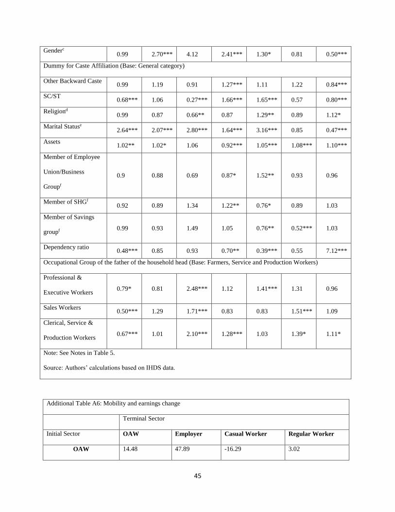
45

Genderc

0.99 2.70*** 4.12 2.41*** 1.30* 0.81 0.50***


Other Backward Caste 0.99 1.19 0.91 1.27*** 1.11 1.22 0.84***

SC/ST 0.68*** 1.06 0.27*** 1.66*** 1.65*** 0.57 0.80***

Religiond

0.99 0.87 0.66** 0.87 1.29** 0.89 1.12*

Marital Statuse

2.64*** 2.07*** 2.80*** 1.64*** 3.16*** 0.85 0.47***

Assets 1.02** 1.02* 1.06 0.92*** 1.05*** 1.08*** 1.10***

Member of Employee

Union/Business

Groupf

0.9 0.88 0.69 0.87* 1.52** 0.93 0.96

Member of SHGf 0.92 0.89 1.34 1.22** 0.76* 0.89 1.03

Member of Savings

groupf 0.99 0.93 1.49 1.05 0.76** 0.52*** 1.03

Dependency ratio 0.48*** 0.85 0.93 0.70** 0.39*** 0.55 7.12***


Professional &

Executive Workers 0.79* 0.81 2.48*** 1.12 1.41*** 1.31 0.96

Sales Workers 0.50*** 1.29 1.71*** 0.83 0.83 1.51*** 1.09

Clerical, Service &

Production Workers 0.67*** 1.01 2.10*** 1.28*** 1.03 1.39* 1.11*



Additional Table A6: Mobility and earnings change

Terminal Sector

Initial Sector OAW Employer Casual Worker Regular Worker

OAW 14.48 47.89 -16.29 3.02

46

Employer -5.03 22.90 -85.63 -12.68

Casual Worker 52.13 71.88 33.30 34.17

Regular Worker 7.57 61.07 22.40 22.40

Notes: See Notes in Table 2.

The numbers reported are percentage change in real earnings associated with change in employment status.


Additional Table A7: Multiple job holding among movers between farm and casual work

Farm work to casual work Casual work to farm work

2004-05 2011-12 2004-05 2011-12

Single Job 76.14 29.17 30.97 61.42

F & S 1.55 1.56

F & W 21.33 68.79 65.55 36.10

S & W 0.43 0.89

F, S & W 0.98 1.61 2.58 0.92

Notes: See Notes in Additional Table A1.

Column Totals add to 100.

Source: Authors calculations based on IHDS data.

SEGMENTATION AND MOBILITY IN THE INDIAN LABOUR MARKETepu/acegd2018/papers/BhaskarJyotiNeog.pdf · 2...

Documents

Transcript of SEGMENTATION AND MOBILITY IN THE INDIAN LABOUR MARKETepu/acegd2018/papers/BhaskarJyotiNeog.pdf · 2...