Sefton Jessop - Getting Performance Out of Risk Parity

UBS Investment Research

Understanding Risk Parity

Getting performance out of risk parity

� Risk parity is fashionable but limited Risk parity is an approach to portfolio construction and asset allocation which iscurrently in vogue. We see two major limitations, however, to the risk parityapproach: it can only be used in a long only framework and it does not allow forthe inclusion of return forecasts.

� Approaching risk parity as a form of robust optimisation In this publication we look at risk parity as a special case of a more general robustoptimisation problem. This more general problem encompasses both meanvariance – minimally robust - and risk parity – maximally robust - as special cases; and overcome the limitations set out above.

� A simple example Our simple simulation example demonstrates that our robust approach has at leasttwo distinct advantages over mean variance. In the presence of estimation error, itgenerates portfolios closer to the true efficient frontier – better performance, and has a lower turnover at monthly rebalancing due to changes in the risk matrix –more stable.

� Risk parity optimisation available in the UBS Portfolio Analysis System The more general approach to using risk parity has been implemented within ourportfolio analysis and risk modelling software: UBS PAS. There is a companionpublication to this, Risk Parity Optimisation in PAS, which details how to use the more general risk parity type optimisation we describe herein with PAS.

Global Equity Research

Global

Quantitative

Quantitative

7 February 2013

www.ubs.com/investmentresearch

David Jessop

[email protected]

+44-20-7567 9882

Claire Jones, CFAAssociate Analyst

[email protected]+44-20-7568 1873

Sebastian Lancetti, CFAAnalyst


Simon StoyeAnalyst


Kenneth TanAnalyst

[email protected]+852-2971 7772

Paul WinterAnalyst


Heran ZhangAssociate Analyst

[email protected]+44 20756 83560

This report has been prepared by UBS Limited ANALYST CERTIFICATION AND REQUIRED DISCLOSURES BEGIN ON PAGE 32. UBS does and seeks to do business with companies covered in its research reports. As a result, investors should be aware that the firm may have a conflict of interest that could affect the objectivity of this report. Investors should consider this report as only a single factor in making their investment decision.

��

mailto:[email protected]

Sanchit Gupta

Sanchit Gupta







Understanding Risk Parity 7 February 2013

UBS 2

Introduction1 Risk Parity as an approach to portfolio construction is currently in fashion. This might simply due to the fact that a few well-known funds, who espouse this technique, have performed very respectably throughout the very volatile conditions of the past few years. However it might be down to the real need for a more robust approach to portfolio construction.

As readers of UBS Quantitative Research have come to expect, we have no intention of simply regurgitating the standard arguments for and against the approach (though we will summarise them shortly for completeness). We shall attempt something – we hope – far more useful. We shall see risk parity as just a very special case of a more general robust portfolio construction framework.

What do we get out of our more general framework as opposed to the risk-parity problem? We can:

(1) Introduce information on expected returns into the problem

(2) We can look at long-short problems (in absolute and benchmark relative space) as well as the long only case used exclusively in risk parity work.

(3) Introduce easily and naturally other investment constraints; such as country, sector neutrality, liability matching, turnover constraints etc.

(4) Look at less extreme robust portfolio problems that might offer a better trade-off between robustness and performance.

We also demonstrate in a simulation exercise, where both the risk matrix and return forecasts are estimated with error, that this approach:

(1) Generates portfolios closer to the efficient frontier than traditional mean variance,

(2) And generates less turnover at monthly rebalancing due to changes in the risk matrix.

And finally all this can be done within our Portfolio Analysis System (UBS-PAS)! Please see the companion note – Risk Parity Optimisation in PAS.

The idea is very simple. In standard portfolio theory, the return to any position is modelled as being equal to the size of that position times its expected return - that is, its return is linear in the weight. We modify this assumption and argue that the return to holding any position will exhibit a diminishing return. Thus holding 10% of the portfolio in a position might be expected to earn, say, a 2% return. However holding 20% will not earn a full extra 4%, but something more than 2 but strictly less than 4%.

Why introduce diminishing returns? There are a number of reasons. They can be seen as a way of incorporating the non-linear aspects of trading costs; taking

1 The authors would like to thank Professor James Sefton of Imperial College, London for the significant contribution he provided to this report.

Sanchit Gupta

Sanchit Gupta

Sanchit Gupta

Sanchit Gupta


UBS 3

larger positions increases transaction costs directly as price impact effects become significant, and taking larger positions reduces portfolio liquidity - an opportunity cost. Secondly, diminishing returns will improve robustness by scaling back the influence of extreme values. Finally, they promote portfolio diversification, and hence increase fund capacity.

We hope that gives you the incentive to read the rest of this note!

A Quick Overview In portfolio construction, all paths start at mean-variance. Mean variance is the search for portfolio weights w that maximise the expected return to a portfolio, T

i iiw wµ µ=¦ (where µ is the vector of expected returns to the

assets) subject to a risk constraint. This constraint is that the volatility of the portfolio, σ(w), is less than some pre-specified target volatility;

Target( ) Tw w wσ σ= Σ ≤ where Σ refers to the risk matrix and σTarget the target

volatility. If the weights of the portfolio are defined in terms of their absolute position, then it is the total volatility of the portfolio that is constrained; if the weights are defined relative to a benchmark, then it is the portfolio’s tracking error that is constrained.

In contrast, in the risk parity problem, the portfolio weights are chosen so that the contributions to risk (or the risk budgets) from each asset are equal2. We give a more detailed definition below. It is argued by its advocates that this approach distributes risk more equally across assets than mean variance and so its performance is more robust. Yet, due the way the problem is set up, it is a very rigid approach, and can only be used for simplest asset allocation problems. This report attempts to show how we can define a more general robust portfolio problem that nests both the mean variance and risk parity problems as special cases; the former being the minimally robust and the latter maximally robust. Further, and this is where we get the pay-off, it allows us to incorporate all the flexibility of mean-variance in the more robust framework of risk parity.

We write down our optimisation problem, which we shall call a robust portfolio optimisation of order k as

1

TTarget

Maximise

subject to w

1 if weights are absoluteand

0 if weights are relative

ki i

i

ii

w

w

cw c

c

µ

σΣ ≤

== ® =¯

¦

¦

2 Please see our report Understanding MCARs (October 2003, Simon Stoye) for a detailed discussion of marginal contributions to risk and their use in decomposing the risk of a portfolio

Mean variance

Standard risk parity

The robust Optimisation Problem

Sanchit Gupta

Sanchit Gupta

Sanchit Gupta


UBS 4

This is mean variance except that in the expression for the portfolio expected return the weight is now raised to the power of 1/k. Therefore when k=1, this is the standard mean-variance portfolio construction problem with an investment constraint. When k>1, we introduce the notion of diminishing returns to holding large positions. The impact of this generalisation is surprisingly dramatic and promotes both diversification and robustness.

As an illustration, suppose you have 2 highly correlated assets with expected returns of 5.1% and 5% (often referred to as the near perfect substitutes problem). In the mean-variance problem, you would choose to take advantage of this near arbitrage opportunity and go very long the slightly higher yielding asset and short the lower yielding one. However if the expected return forecasts were reversed – which amounts to a small change in the forecasts - the optimal portfolio positions would be reversed too – which amounts to a large change in portfolio weights! This is one of the well documented difficulties with mean-variance; small changes in forecasts cause large shifts in portfolio positions; and is one of the principal reasons the approach is not regarded as robust. In contrast with diminishing returns, say k=3, you will choose to hold close to 50% in both assets, and if the forecasts are reversed the portfolio positions will only alter marginally too! Though this is a rather prosaic example, it illustrates the two problems can have very different solutions, and that introducing diminishing returns could offer significant improvements in robustness.

Now we shall show that this problem framework encompasses the risk parity problem. The risk parity portfolio allocates an equal risk budget to each asset; where the risk budget has its standard definition as the Weighted Marginal Contribution to Risk. The Marginal Contribution to Risk (MCR) of an asset is defined as the marginal change in the portfolio’s volatility for a marginal change in the weight of the asset, that is

( )w ii T

i

VwMCRw w Vwσ∂= =

∂

where the notation (.)i denotes the ith element of a vector. The weighted marginal contribution to risk is simply the asset’s weight multiplied by its MCR, that is wiMCRi. These weighted MCRs are called the risk budgets and can be thought of as a decomposition of the portfolio risk as the sum of the weighted MCRs across all assets equals the total risk of the portfolio3. The risk parity problem searches for the portfolio where the weighted MCRs of each position are equal.

How does our general problem encompass this rather idiosyncratic one? On page 18 we will derive the first order conditions (i.e. the equation our optimal solution weights must satisfy) for our generalised optimisation problem but for now we simply quote it. The first order condition for each asset i is

1 ( )iki i i T

Vww ww Vw

λµ κ§ ·

= −¨ ¸© ¹

3 This follows immediately from the above formula for

( ) TTi i

i i T Ti

w Vw w Vww MCR w Vww Vw w Vw

= = =¦

k = 1 gives us mean variance …

Definition of risk parity

Fitting risk parity into our framework

Sanchit Gupta

Sanchit Gupta


UBS 5

where the constants λ and κ are the Lagrange multipliers corresponding to the two constraints in the general optimisation problem. It is not difficult to show that one can always choose a target volatility σTarget such that the multiplier κ=0. Hence if the expected returns are equal, µi= µ for all i, the first order conditions simplify to

1 ( )iki i i iT

Vww w w MCRw Vw

λµ = =

Hence our robust problem is equivalent to a risk parity problem as k→∞ .

To summarise then, when k=1, our problem is mean variance. We regard this as the minimally robust case. As k increases, our problem trades off a little performance for both diversification and robustness. As k→∞ the problem becomes equivalent to risk parity problem which can be regarded as a maximally robust problem.

However, because we have phrased the problem as a slight modification of the textbook mean-variance problem, all the usual bells and whistles that can be added to the mean-variance problem can be added to our problem, too. Thus we can introduce turnover constraints, risk exposure constraints, examine long-short problems etc.

.

We can cope with negative weights too


UBS 6

The Success of Risk Parity Bridgewater’s All Weather Fund is the first fund credited with adopting the risk-parity approach to portfolio construction. According to Bridgewater ‘risk parity is about balance’; it is about ‘balancing one’s risk exposures’ across assets to achieve ‘consistent performance’. Over the last few years, many other funds have adopted this technique.

The motivation is simple. In a standard asset allocation portfolio with 60% invested in equities and 40% invested in bonds, around 90% of the risk emanates from the equity component. Equities are just much more volatile than bonds. Hence balancing the risks leads to a portfolio more heavily invested in bonds. However if it is required that this risk balanced fund is to have a similar level of risk to a standard 60-40 allocation, it is then necessary to leverage up the positions.

There are many recent papers (e.g. Allen (2010), Foresti and Rush (2010)) showing that such an allocation would have outperformed the more traditional allocation over the last 30 years. This has led to enormous interest in the approach. However, Anderson et al (2011) show in a very long back-test that although risk parity outperformed over the whole period “levered risk parity underperformed during a relatively long sub period” and “transaction costs negated the gains over the full 85-year horizon”.

More recently Asness and Pedersen (2012) have offered a reason for the outperformance of these risk parity funds. They argue that investors are leverage averse; hence return seeking investors tend to bid up assets with a high risk premium relative to those with a low premium. This flattens the security market line, implying that investors willing to use leverage can earn a higher risk adjusted return.

The risk parity approach is not without its critics; see Inker (2010), O’Gorman (2012). Here we summarise the principal criticisms;

(1) Risk Parity asset allocation strategies allocate far more weight to bonds in their portfolio. As we have seen a bull run to bonds over the last 30 years, it is not surprising that these allocations have outperformed. More importantly, though, with yields at historic lows surely this run cannot continue.

(2) Risk Parity asset allocation strategies can use substantial leverage. This leverage comes with a risk and can make the strategies vulnerable to a market turns and significant draw-downs.

(3) The approach offers no guidance as to what assets should be included in the strategy. Given a particular asset class you are either in or out – there is no half-way house. Thus if the decision is taken to hold commodities in the portfolio, the strategy will hold a considerable weight in commodities as it is given the same risk budget as equities and bonds.

(4) Risk Parity does not use any information on expected returns. Thus the allocation to commodities will be the same as equities (in risk terms) even though the risk premiums are very different.

Risk parity in asset allocation

Sanchit Gupta

Sanchit Gupta

Sanchit Gupta

Sanchit Gupta

Sanchit Gupta


UBS 7

(5) It is a heuristic approach – there is no real fundamental rationale (though we believe we offer something of a rationale in this paper). So why prefer this heuristic over others such as minimum variance, equally weighting and so on?

Sanchit Gupta


UBS 8

An experiment to show that this approach works The idea of introducing diminishing returns in the performance measure is a simple extension, but it does have strong implications. We believe the best way to explore these ideas is through an example. We start by discussing the problem of portfolio construction in the face of estimation error. We then show how our robust approach to portfolio construction delivers better performance than mean variance optimisation in the face of this estimation error.

Our example is inspired by the work of Broadie (1993). If one knew the ‘true’ underlying process driving equity returns, portfolio construction would be easy. The difficulty arises because one must use estimates; in practise build a risk matrix and forecast expect returns. These estimates are subject to error, and if your portfolio construction process is very sensitive to these errors, your chosen portfolio might be very different from a desired portfolio (the portfolio you would have held in you had know the truth).

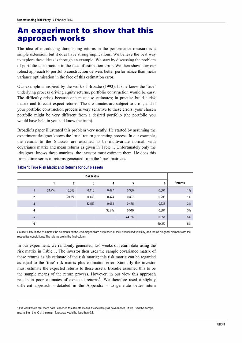
Broadie’s paper illustrated this problem very neatly. He started by assuming the experiment designer knows the ‘true’ return generating process. In our example, the returns to the 6 assets are assumed to be multivariate normal, with covariance matrix and mean returns as given in Table 1. Unfortunately only the ‘designer’ knows these matrices, the investor must estimate them. He does this from a time series of returns generated from the ‘true’ matrices.

Table 1: True Risk Matrix and Returns for our 6 assets

Risk Matrix

1 2 3 4 5 6 Returns

1 24.7% 0.308 0.413 0.477 0.380 0.304 1%

2 29.6% 0.430 0.474 0.397 0.298 1%

3 32.5% 0.062 0.475 0.336 3%

4 33.7% 0.519 0.384 3%

5 44.6% 0.351 5%

6 60.2% 5%

Source: UBS. In the risk matrix the elements on the lead diagonal are expressed at their annualised volatility, and the off diagonal elements are the respective correlations. The returns are in the final column

In our experiment, we randomly generated 156 weeks of return data using the risk matrix in Table 1. The investor then uses the sample covariance matrix of these returns as his estimate of the risk matrix; this risk matrix can be regarded as equal to the ‘true’ risk matrix plus estimation error. Similarly the investor must estimate the expected returns to these assets. Broadie assumed this to be the sample means of the return process. However, in our view this approach results in poor estimates of expected returns4. We therefore used a slightly different approach - detailed in the Appendix – to generate better return

4 It is well known that more data is needed to estimate means as accurately as covariances. If we used the sample means then the IC of the return forecasts would be less than 0.1.


UBS 9

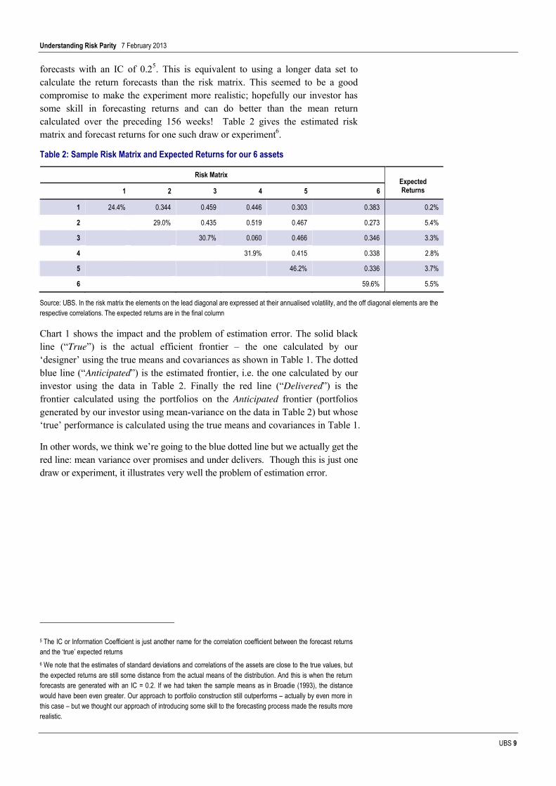
forecasts with an IC of 0.25. This is equivalent to using a longer data set to calculate the return forecasts than the risk matrix. This seemed to be a good compromise to make the experiment more realistic; hopefully our investor has some skill in forecasting returns and can do better than the mean return calculated over the preceding 156 weeks! Table 2 gives the estimated risk matrix and forecast returns for one such draw or experiment6.

Table 2: Sample Risk Matrix and Expected Returns for our 6 assets

Risk Matrix

1 2 3 4 5 6 Expected Returns

1 24.4% 0.344 0.459 0.446 0.303 0.383 0.2%

2 29.0% 0.435 0.519 0.467 0.273 5.4%

3 30.7% 0.060 0.466 0.346 3.3%

4 31.9% 0.415 0.338 2.8%

5 46.2% 0.336 3.7%

6 59.6% 5.5%

Source: UBS. In the risk matrix the elements on the lead diagonal are expressed at their annualised volatility, and the off diagonal elements are the respective correlations. The expected returns are in the final column

Chart 1 shows the impact and the problem of estimation error. The solid black line (“True”) is the actual efficient frontier – the one calculated by our ‘designer’ using the true means and covariances as shown in Table 1. The dotted blue line (“Anticipated”) is the estimated frontier, i.e. the one calculated by our investor using the data in Table 2. Finally the red line (“Delivered”) is the frontier calculated using the portfolios on the Anticipated frontier (portfolios generated by our investor using mean-variance on the data in Table 2) but whose ‘true’ performance is calculated using the true means and covariances in Table 1.

In other words, we think we’re going to the blue dotted line but we actually get the red line: mean variance over promises and under delivers. Though this is just one draw or experiment, it illustrates very well the problem of estimation error.

5 The IC or Information Coefficient is just another name for the correlation coefficient between the forecast returns and the ‘true’ expected returns 6 We note that the estimates of standard deviations and correlations of the assets are close to the true values, but the expected returns are still some distance from the actual means of the distribution. And this is when the return forecasts are generated with an IC = 0.2. If we had taken the sample means as in Broadie (1993), the distance would have been even greater. Our approach to portfolio construction still outperforms – actually by even more in this case – but we thought our approach of introducing some skill to the forecasting process made the results more realistic.


UBS 10

Chart 1: Efficient frontiers

Source: UBS. The True efficient frontier is calculated using the true data in Table 1. The Anticipated frontier is calculated using the estimated data in Table 2. The Delivered frontier is the frontier generated using the portfolios on the anticipated frontier but with the performance calculated using the true data.

As an interesting aside, we note that the estimated minimum variance portfolio lies quite close to the actual minimum variance portfolio. As we move along the curve and take our return estimates more into account then the distance between the Delivered and True frontier increases. This is, in a picture, part of the justification for minimum variance investing; generally your estimates of risk are much better than your estimates of return and so you can get closer to the efficient frontier and deliver better performance by effectively ignoring your return estimates.

Comparison of approaches to portfolio construction? We chose 3 points on the efficient frontier to analyse, targeting a volatility of 24%, 26% and 28%; a low, medium and high risk portfolio. The method is as follows. Using the procedure in the previous section, we generate an estimated risk matrix and a set of return forecasts. From these, we build a mean-variance portfolio (MV) and a maximally robust portfolio (RP) that maximises performance subject to the risk limits of 24%, 26% and 28%. As in the previous section, we then calculate the delivered performance of these portfolios using the ‘true’ risk and return matrices. This gives a single data point. We then repeat this a 1000 times, to establish average performance of these difference portfolio construction approaches in the face of estimation error.

Results

We illustrate the results of 1000 simulations in Chart 2 and Chart 3 for the maximally robust and mean variance portfolios when the target volatility is 26%. We can see in the charts that the distribution of maximally robust portfolios looks to be far closer to the efficient frontier than the mean variance portfolios. But how can we quantify this?

Sanchit Gupta


UBS 11

Chart 2: Distribution of maximally robust portfolios targeting a volatility of 26%

Chart 3: Distribution of mean variance portfolios targeting a volatility of 26%

Source: UBS Source: UBS

First we use two informal measures to compare the performance of the portfolios construction process. The first is the average distance in risk-return space of the portfolios to the point on the efficient frontier with the respective target volatility7.

Chart 4: Distance measures we use

Source: UBS

The second is the average distance of the portfolios to the respective nearest point on the efficient frontier. Thus in Chart 4, for the example portfolio (Green point), Distance 1 is the distance to the point on the efficient frontier with desired target volatility, and Distance 2 is distance to the nearest point on the efficient frontier.

Table 3 shows the median distances for the various portfolios under the three measures described above. The maximally robust portfolios are closer to both

7 Where we measure distance as the usual Euclidian measure.


UBS 12

the target risk point on the efficient frontier and to the efficient frontier in general.

Table 3: Median distances from the simulated portfolios

Distance 1: Average distance to point on frontier with required

target volatility Distance 2: Average distance to nearest point on frontier

Maximally Robust Portfolio Mean-Variance Portfolio Maximally Robust Portfolio Mean-Variance Portfolio

Target Volatility of 24% 1.25 1.49 0.66 0.84



Source: UBS. The table shows the median distances from the simulated portfolios to the True portfolio (i.e. the portfolio calculated using the actual parameters), the MV portfolio with the same risk constraint and the nearest point on the efficient frontier. Distances are effectively in % return units; thus a distance of 1 is equivalent to 1% in the return units or 1% in risk units.

Though informative, the distance unit in risk-return space can only be used as an informal guide. To do it more formally requires a more rigorous approach to weighting risk and return. Assume our investor chooses a portfolio w, and assume his utility from owning this portfolio is measured by the function

( ) 21 1 T TT w w Vw

w rE e eλλ µλ

λ λ

§ ·− −¨ ¸− © ¹− −=

where λ is the parameter of risk aversion and the equality follows form the fact that the returns, r, are normally distributed. This utility function is called a Constant Absolute Risk Aversion (CARA) utility function and is arguably the

standard the asset-pricing literature. The term 2

T Tw w Vwλµ − is referred to as

the certainty equivalent return (CER). It is the level of certain (or guaranteed) return one would exchange for the exposure to a higher but uncertain return. Effectively it weights together return and variance using the parameter of risk aversion. But what risk aversion should we use? This is easy. When comparing the mean-variance and maximally robust portfolios, we use the risk aversion parameter that would imply we would hold the portfolio on the efficient frontier with that respective target volatility (if we knew the true risk and return matrices)8

Chart 5 to Chart 7 shows the empirical cumulative density functions for the CERs for the three different target volatilities. With respect to the middle case, Chart 6, the red describes the performance of the robust portfolio approach. It says that the robust portfolio delivers a CER less than 0% roughly 12.5% of the time; a CER less than 0.05% roughly 50% of the time, and a CER of less than 1% 87% of the time. In contrast mean-variance delivers a CER of less than 0% 37% of the time, less than 0.05% about 70% of the time and a CER of less than 1% 90% of the time. In short, one can say that the maximally robust portfolio construction technique stochastically dominates mean-variance in that whatever your choice of CER level, it is more likely that robust portfolio construction will deliver this return than mean-variance.

8 For this example, a target volatility of 24% corresponds to a λ of 1.03, a volatility of 26% a λ of 0.64 and a volatility of 28% a λ of 0.46.

Certainty equivalent return


UBS 13

Chart 5: 24% risk – cumulative density Chart 6: 26% risk – cumulative density Chart 7: 28% risk – cumulative density

Source: UBS. Charts show the cumulative density functions for the CER for the simulated portfolios.

So how much better is the maximally robust portfolio technique? We could ask how much cost in return units would an investor be willing to pay to use the robust portfolio technique relative to mean variance. Denote the cost as c and the portfolio built using our robust approach as wRP and the portfolio built using mean-variance as wR .Then this cost can be estimated as the level solving the following equation

2 21 1RP RP RP MV MV MVw w Vw c w w VwE e E e

λ λλ µ λ µ

λ λ

§ · § ·− − − − −¨ ¸ ¨ ¸© ¹ © ¹

§ · § ·− −=¨ ¸ ¨ ¸¨ ¸ ¨ ¸© ¹ © ¹

where the expectation is with respect to the 1000 simulations. The Table below gives the results for the three different target volatilities.

Table 4: A measure of the value in % return units of the robust portfolio construction technique relative to mean variance.

Target Volatility 24% 26% 28%

Difference 0.22% 0.34% 0.43%

Source: UBS

As the average return to the portfolios in these three cases is roughly 2.4%, 2.6% and 2.75% and an investor can get 1.6% from the minimum variance portfolio, we could argue that the our robust portfolio approach gives a performance uplift of 34% (= 0.34/(2.6-1.6)), which is considered valuable.


UBS 14

Testing the sensitivity of the solution to changes in the covariance matrix The second test we undertook was to investigate the sensitivity of the solution weights to a change in the covariance matrix. When creating the random return series we generated an extra four weeks of returns (so 160 in total) and then calculated two covariance matrices: one from the first 156 data points and one from the last 156 data points, so moving the calculations forward by one month.

We ran two sets of optimisations using these two covariance matrices together with the true returns and measured the turnover between the two groups of resulting portfolios.

Table 5 shows the results from 1000 simulations9. What is pleasing from our point of view is that the robust portfolios have a lower turnover than the mean variance portfolio with the same risk. The turnover falls as we increase the risk as for these higher risk portfolios the relative importance of the (unchanging) returns against the (changing) risk matrices increases.

Table 5: Turnover due to changes in the covariance matrix

1st Qu. Median 3rd Qu.

Maximally Robust Portfolio – Target Volatility 24% 2.31% 3.67% 5.77%

Maximally Robust Portfolio – Target Volatility 26 % 1.67% 2.66% 4.25%

Maximally Robust Portfolio – Target Volatility 28% 1.13% 2.04% 3.48%

Mean Variance Portfolio – Target Volatility 24% 3.56% 5.61% 8.68%



Source: UBS. The table shows the summary statistics of the two way monthly turnover.

9 The minimum variance portfolio (unreported) has a much higher turnover than any of the maximally robust portfolios.


UBS 15

A Robust Approach to Portfolio Optimisation Risk Parity has so far only been applied to long-only asset allocation problems where there are a few assets and no investment constraints. As we have already outlined, our aim is to nest both the risk-parity approach and the mean variance approach in the same generalised framework and so overcome these limitations. It turns out that mean-variance can be regarded as minimally robust and risk parity as maximally robust in this framework.

The pay-off is that because this framework is very general, long-short and benchmark relative problems as well as all the various investment constraints used by practitioners can be easily incorporated too; therefore making a risk parity based approach far more flexible. Perhaps surprisingly – given risk parity is exclusively concerned with risk - we do this by introducing a slightly modified performance measure whilst leaving the risk measure unchanged! Simply, it proves easier to place risk parity into the standard optimisation framework by modifying the return measure rather than risk measure.

First though we introduce our risk measure. We base our notation on Maillard, Roncalli and Teiletche (2010) as closely as possible.

Contribution to Risk Consider a portfolio of weights w = (w1, w2, ..., wn) in the n securities. Let the covariance (or risk) matrix of return to these assets be Σ with elements σij . Then the volatility of the portfolio is

( ) Tw w wσ = Σ

The marginal contribution to risk (MCR) is defined to be the increase in volatility for a marginal increase in the position in security i

( )( )

w ii

i

wMCR

w wσ

σΣ∂= =

∂

where (.)i denotes the ith element of the vector. In a standard mean variance portfolio construction problem, the marginal contribution to risk from each asset is equated to their marginal returns.

The weighted marginal contribution to risk – referred to more simply as the contribution to risk or just the risk budget and is defined as

( )( ) :

( )i i

i i i

w ww w MCR

wσ

σΣ

= =

The contribution to risk satisfies the identity that their sum is the total volatility of the portfolio

( ) ( )ii

w wσ σ=¦


UBS 16

This is motivation for the term risk budget. It is a linear decomposition of the risk of the portfolio into the contribution from each of its positions.

The Risk Parity portfolio problem is the search to find the weights w such that the contribution to risk from each asset is equal. Thus in risk parity the aim is to share the risk budget equally between each of the assets.

A criticism of this approach has been that it is just a heuristic approach to portfolio construction, in that there is no clear overall performance objective. The manager adopts a rule to share out his risk budget evenly between the assets. The only control as such the manager has over the resulting portfolio is the choice of whether to include the asset in the optimisation. In particular, no importance is given to expected returns. We address this in the next section.

Contribution to Return Denote the expected return to the securities by the n-vector µ.. We shall define the robust return function of order k as

( ) ( ) ( )1

, , where , ki i i i

ir k w r k w r k w wµ= =¦

where k=1, 3, 5, ... Thus the robust return function is also a sum of the individual return contributions, ri(k,w). We focus on the odd integers for k only as then the return function is well defined for negative weights, too. This is so our formulation applies equally well to the case of long-short portfolios as it does to long only. However, with very little effort, one could adapt the notation so that the function is well behaved for all k>=1. All that is required is that the function, f(w) is continuous around 0, and that f(-w)=-f(w). Though simple, the notation is a little clumsy, so we stick with the odd integers.

We shall now motivate this choice of return function. When k = 1, the robust return function is just the standard linear return function used in mean-variance analysis; there is no diminishing return to the asset. Thus doubling the position doubles the expected return.

For larger k, there is now a diminishing return to holding more of any security i. Thus doubling a position no longer doubles its return contribution; the marginal contribution to return from increasing your position in any asset falls off as the size of the position increases.

In Chart 8 we plot the contribution to return as a function of the weight in security i for different values of k. As k increases, the benefits of holding a large position in any asset diminish rapidly. Thus the impact of having diminishing returns will be to shrink positions back towards a more equally weighted portfolio. It is in this sense that the approach is considered robust; it behaves in a similar way to a James-Stein or Bayesian shrinkage approach.


UBS 17

Chart 8: Contribution to Return for different order k

0.0%

0.2%

0.4%

0.6%

0.8%

1.0%

1.2%

1.4%

1.6%

0.00% 0.20% 0.40% 0.60% 0.80% 1.00% 1.20% 1.40% 1.60% 1.80% 2.00%

Cont

ribut

ion

to Re

turn

Weight invested inSecurity i

k= 1

k=3

k=5

k=9

Increasing k

Source: UBS

How could one theoretically justify this robust performance measure? Though we have no intention of building up this function from micro-foundations, we can see a number of reasons why there are diminishing returns to taking a large position in any asset. The most obvious involve the implicit trading and liquidity costs in holding a large position.

(1) As an investor builds up a position, it will cost him a more to trade out of this position due to direct market impact costs of the trade. Work on modelling these costs – see for example Kissell (2008), Almgren (2005) – suggest these costs rise almost linearly with the size of the position. Hence, if the expected return is net of these costs, the return derived from holding the asset will diminish with the size of the position.

(2) Similarly the size of the position will have an impact on the ability of the manager to change his portfolio positions quickly if new information becomes available. This loss of liquidity clearly has a cost too and will be a function of the size of the individual portfolio positions.

One might also argue that there are more indirect costs of holding large positions,

(3) Taking a large position in an asset runs the risk of reputational loss and ensuing funds outflow if that position does particularly badly. This is always the risk of ‘putting all your eggs in a one basket’. If the manager is risk averse, this will induce a diminishing return to taking large positions.

Hence the diminishing marginal returns model of performance could be justified as a reduced form model of expected returns net of trading, liquidity and reputational costs.

An alternative approach to justifying diminishing return performance measures could be based on the work of Ferson and Siegel (2001) in the Journal of Finance.


UBS 18

(4) Asset managers are generally judged on their unconditional or average performance over long periods. They therefore should pursue a strategy of maximising their average performance, not their instantaneous performance. This implies that if there are assets with high returns, managers should use this opportunity to reduce risk. This effectively introduces a diminishing marginal return performance function (their figure 1 on page 971).

This paper then goes onto remark how their performance function is similar to the empirically motivated robust estimators of Hampel (1974), Carroll (1989).

(5) Robust estimators limit the influence of extreme signal observations. Introducing diminishing influence (or return) functions results in portfolios that are likely to be robust to estimation errors in expected returns. This conjecture is supported by the out-of-sample experiments of Bekaert and Liu (2004) and Ferson and Siegel (2003).

A major appeal of this problem specification is that it encompasses the risk parity approach to portfolio optimisation. The robust return function has a well behaved limit as k tends to infinity. This follows immediately from the following relationship

( )1

log lim 1ki ik

w k w→∞

§ ·= −¨ ¸

© ¹

Thus maximising the robust return function r(∞,w) is equivalent to maximizing the function

( )logi ii

wµ¦

as these two functions are just affine transformations of each other. As Maillard, Roncalli and Teiletche (2010) show (and we intend to, also) maximizing this function subject to a risk constraint delivers the RP portfolio when expected returns are equal. The RP portfolio can therefore be regarded as a special case of robust portfolio optimisation, or in some sense as a maximally robust approach.

Optimisation We can now set out the optimisation problem; maximising the robust return subject to a risk and investment constraint

We define the Lagrangian of the problem of maximizing r(k,w) subject to the risk of the portfolio, σ(w), being less than the target risk of as

( ) ( )( )Targetmax , ( 1)T

wL r k w w e wλ σ σ κ= − − − − (1)

where λ and κ are the Lagrangian multipliers associated with the risk and investment constraint respectively and e is a vector of 1s. The first order condition of optimality is therefore

( ),ii

i

r k wMCR

wλ κ= +

(2)


UBS 19

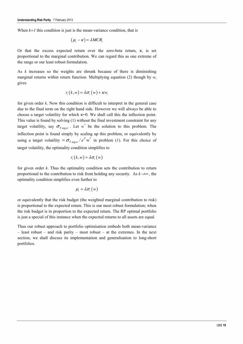
When k=1 this condition is just is the mean-variance condition, that is

( )i iMCRµ κ λ− =

Or that the excess expected return over the zero-beta return, κ, is set proportional to the marginal contribution. We can regard this as one extreme of the range or our least robust formulation.

As k increases so the weights are shrunk because of there is diminishing marginal returns within return function. Multiplying equation (2) though by wi gives

( ) ( ),i i ir k w w wλσ κ= +

for given order k. Now this condition is difficult to interpret in the general case due to the final term on the right hand side. However we will always be able to choose a target volatility for which κ=0. We shall call this the inflection point. This value is found by solving (1) without the final investment constraint for any target volatility, say etT argσ . Let w* be the solution to this problem. The

inflection point is found simply by scaling up this problem, or equivalently by using a target volatility *

arg / weTetTσ= in problem (1). For this choice of

target volatility, the optimality condition simplifies to

( ) ( ),i ir k w wλσ=

for given order k. Thus the optimality condition sets the contribution to return proportional to the contribution to risk from holding any security. As k→∞ , the optimality condition simplifies even further to

( )i i wµ λσ=

or equivalently that the risk budget (the weighted marginal contribution to risk) is proportional to the expected return. This is our most robust formulation; when the risk budget is in proportion to the expected return. The RP optimal portfolio is just a special of this instance when the expected returns to all assets are equal.

Thus our robust approach to portfolio optimisation embeds both mean-variance – least robust – and risk parity – most robust – at the extremes. In the next section, we shall discuss its implementation and generalisation to long-short portfolios.


UBS 20

A detailed look at the portfolios The idea of introducing diminishing returns in the performance measure is a simple extension, but it does have strong implications. We believe the best way to explore these ideas is through an example. We shall first discuss the long only or asset allocation case. Then we turn to the long-short case. Our final example is a more extended simulation which highlights some of the features of the extended risk parity solution.

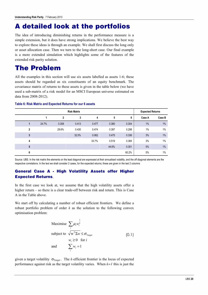
The Problem All the examples in this section will use six assets labelled as assets 1-6; these assets should be regarded as six constituents of an equity benchmark. The covariance matrix of returns to these assets is given in the table below (we have used a sub-matrix of a risk model for an MSCI European universe estimated on data from 2008-2012).

Table 6: Risk Matrix and Expected Returns for our 6 assets

Risk Matrix Expected Returns

1 2 3 4 5 6 Case A Case B

1 24.7% 0.308 0.413 0.477 0.380 0.304 1% 1%

2 29.6% 0.430 0.474 0.397 0.298 1% 1%

3 32.5% 0.062 0.475 0.336 3% 1%

4 33.7% 0.519 0.384 3% 1%

5 44.6% 0.351 5% 1%

6 60.2% 5% 1%

Source: UBS. In the risk matrix the elements on the lead diagonal are expressed at their annualised volatility, and the off diagonal elements are the respective correlations. In the text we shall consider 2 cases, for the expected returns; these are given in the last 2 columns

General Case A - High Volatility Assets offer Higher Expected Returns.

In the first case we look at, we assume that the high volatility assets offer a higher return – so there is a clear trade-off between risk and return. This is Case A in the Table above.

We start off by calculating a number of robust efficient frontiers. We define a robust portfolio problem of order k as the solution to the following convex optimisation problem:

1

TTarget

Maximise

subject to w

0 for and 1

ki i

i

i

ii

w

ww i

w

µ

σΣ ≤≥

=

¦

¦

(0.1)

given a target volatility σTarget . The k-efficient frontier is the locus of expected performance against risk as the target volatility varies. When k=1 this is just the


UBS 21

standard long-only mean-variance efficient frontier. This is the blue (highest) line plotted in the diagram below.

Chart 9: The efficient frontiers for k=1,3,5,11,∞

1

1.5

2

2.5

3

3.5

4

4.5

5

21.3% 23.6% 26.0% 28.4% 30.8% 33.1% 35.5% 37.9% 40.3%

Mean Variance

k=3

k=5

k=11

k = Infinity

3

3.2

3.4

3.6

3.8

4

4.2

27.0% 27.9% 28.9% 29.8% 30.8% 31.7%

YY

X

X

1

1.5

2

2.5

3

3.5

4

4.5

5

21.3% 23.6% 26.0% 28.4% 30.8% 33.1% 35.5% 37.9% 40.3%

Mean Variance

k=3

k=5

k=11

k = Infinity

3

3.2

3.4

3.6

3.8

4

4.2

27.0% 27.9% 28.9% 29.8% 30.8% 31.7%

YY

X

X

Source: UBS

We can highlight 2 points on this frontier. The frontier starts in the bottom left hand corner at the minimum variance portfolio. This portfolio has a risk of 21.2% and return of 1.27%. In the top right hand corner is the maximum return portfolio which is invested entirely in assets 5 and 6; it has risk of 41% and a return of 5%.

The other frontiers on the chart plot the corresponding achieved risk-return trade-off for k-robust frontiers when k=3, 5, 11 and∞. These frontiers all lie below the mean-variance frontier; some performance has been sacrificed for greater diversification. However, in this example, the sacrifice is small. (Obviously if the frontiers were plotted instead in the risk versus robust return space - where robust return is measured 1 kwµ - then the respective k frontier would be the envelope frontier with all the others lying below).

Now where an investor chooses to be on the risk return frontier depends on their preferences. However we wish to know about the properties of the portfolios on these different frontiers. We therefore cut across the frontiers either keeping risk constant (line X-X in the inset) or return constant (line Y-Y in the inset). Both cuts pass through the same point on k=∞ frontier. This point was chosen as it is the unique point on the k=∞ frontier where the weighted marginal contribution to risk from each asset is equal to the expected return. We shall call this point the inflection point. It was defined precisely in the previous section.


UBS 22

Table 7 and Table 8 below give details of the portfolio weights, the weighted and unweighted marginal contribution to risks of the portfolios on the frontiers for these 2 cuts. In Table 7 (the vertical cut X-X) the risk is held constant at 28.6%. The mean-variance portfolio delivers an expected return of 3.51% with the portfolio on the k=∞ frontier delivering a lower expected return of 3.42%. Though the expected return difference is not very great, the portfolio weights vary considerably. (This is the point made forcibly by Mark Kritzman (2006) that two portfolios can look very different but have a very similar expected performance). In the mean variance efficient portfolio, 60% of the portfolio weight is concentrated in assets 3 and 5. In contrast, in the robust portfolios only allocate 40%. This the principal impact of including a diminishing marginal return to holding any asset; as the holding becomes larger there is less and less benefit to increasing the weight any further and as a result the optimal portfolio are more diversified.

Table 7: The Portfolio weights, MCR and weighted MCR along the line X-X

Mean-Variance (k=1) Robust Portfolio, k = 3 Robust Portfolio, k = 5 Robust Portfolio, k = ∞

Risk = 28.6%, Return = 3.51% Risk = 28.6%, Return = 3.44% Risk = 28.6%, Return = 3.42% Risk = 28.6%, Return = 3.417%

µi Weights MCR Weighted MCR Weights MCR Weighted

MCAR Weights MCR Weighted MCR Weights MCR Weighted

MCR

1 1% 0.135 0.146 0.02 0.112 0.143 0.016 0.112 0.142 0.016 0.112 0.142 0.016

2 1% 0 0.154 0 0.079 0.17 0.013 0.085 0.171 0.015 0.092 0.172 0.016

3 3% 0.307 0.258 0.079 0.215 0.24 0.052 0.208 0.239 0.05 0.202 0.237 0.048

4 3% 0.166 0.258 0.043 0.186 0.26 0.048 0.185 0.26 0.048 0.184 0.259 0.048

5 5% 0.280 0.369 0.103 0.236 0.353 0.084 0.232 0.352 0.082 0.228 0.349 0.079

6 5% 0.111 0.369 0.041 0.172 0.427 0.074 0.177 0.431 0.076 0.182 0.436 0.079

Source: UBS Quants

From the table, we can assess the impact of introducing the diminishing marginal return function on the respective un-weighted and weighted marginal contributions to risk of any asset. The first order condition for optimality in all these optimization problems is

( )1

MCR

iki i i T

ww w

w wµ λ κ

§ ·¨ ¸Σ

= +¨ ¸Σ¨ ¸¨ ¸

© ¹��

where λ, κ are constants (the Lagrangian multipliers for the risk and investment constraints respectively). For the mean-variance case, k=1, the optimisation sets the expected returns to a security proportional to its marginal contribution to risk (MCR) plus a constant κ; in this particular example κ =-0.09 and λ=0.17. (The term wi on the left and right hand side cancels when k = 1). This equality is clear in the table as the 2nd column of expected returns µi, is proportional to MCR of each asset in column 4 (on the proviso that the portfolio weight is greater than zero).

In contrast for the maximally robust case, k=∞, the optimisation sets the expected returns proportional to the weighted marginal contribution to risk plus


UBS 23

a constant (The term wi1/k on the left hand of the equation tends to 1 as k tends to

∞). We chose the line X-X so that this constant is zero κ =0.0 – the inflection point - and λ=0.6. To check this, note that the 2nd column of expected returns µi, is proportional to portfolio weighted MCR in the final column of the table. Thus in the mean variance portfolio returns are related to MCRs, whereas in the robust portfolio returns are related to their risk budgets.

The other two cases corresponding to k =3, 5 are also documented in the table. It is evident that these cases lie between the extremes.

In Chart 10, we look at weighted MCR of the assets as one moves along the k-efficient frontier when k=∞. For very low risk, the portfolio approximates the minimum variance portfolio with the entire portfolio’s risk budget allocated to the low volatility assets. As we move along the frontier, relaxing the target volatility, more of the risk budget is allocated to the volatile but higher return assets. There is a unique value for the target volatility (marked by A-A in the figure) where the risk budgets are precisely proportional the expected returns. This is the inflection point. Though analytically ‘neat’, we believe there is little special about this point. An investor should choose their preferred point on the frontier based on their desired risk to return trade-off.

Finally as the target volatility is relaxed further, the optimisation allocates even more of the risk budget to the high volatility assets. However it reaches the maximum adjusted return – not when it has allocated all its weight to highest yielding asset as in the mean variance case – but when the portfolio weights are proportional to the vector of expected returns.

Chart 10: Weighted marginal contribution to risk for each of 6 assets

0.00

0.02

0.04

0.06

0.08

0.10

0.12

0.14

0.16

21.3% 23.6% 26.0% 28.4% 30.8% 33.1% 35.5% 37.9% 40.3%

Portfolio Risk

Weig

hted M

CAR

Asset 1

Asset 2

Asset 3

Asset 4

Asset 5

Asset 6

A

A

Source: UBS. The line A-A shows the level of risk where the weighted marginal contributions to risk are proportional to the returns.

In Table 8 we detail similar results for the horizontal cut (Y-Y) in Chart 9. Returns to each portfolio are now all equal to 3.42%. The mean-variance portfolio achieves this return with a risk of 28.1%, whereas the robust portfolios


UBS 24

have a slightly higher risk around 28.6%. The story for this cut is similar; the performances of the portfolios are only slight different but this belies large difference in the asset weights.

Table 8: The Portfolio weights, MCR and weighted MCR along the line Y-Y


Risk = 28.1%, Return = 3.42% Risk = 28.5%, Return = 3.42% Risk = 28.6%, Return = 3.42% Risk = 28.6%, Return = 3.42%

µi Weights MCR Weighted MCR Weights MCR Weighted

MCAR Weights MCR Weighted MCR Weights MCR Weighted

MCR

1 1% 0.164 0.151 0.025 0.116 0.144 0.017 0.114 0.143 0.016 0.112 0.142 0.016

2 1% 0 0.154 0 0.081 0.17 0.014 0.086 0.171 0.015 0.093 0.172 0.016

3 3% 0.303 0.259 0.078 0.215 0.241 0.052 0.209 0.239 0.05 0.202 0.237 0.048

4 3% 0.163 0.259 0.042 0.185 0.261 0.048 0.185 0.26 0.048 0.184 0.259 0.048

5 5% 0.265 0.366 0.097 0.233 0.353 0.082 0.231 0.351 0.081 0.228 0.349 0.079

6 5% 0.105 0.366 0.038 0.169 0.426 0.072 0.175 0.431 0.075 0.182 0.436 0.079

Source: UBS Quants

Risk Parity - Case B - Expected Returns to each Asset are Equal

The risk parity problem is a special case of our generalised problem when the returns to each asset are the equal. Hence we shall quickly look at Case B in Table 6 when the expected return to each asset is 1%.

Under this assumption, the mean-variance frontier collapses to a single point – the minimum variance portfolio. However the other k-efficient frontiers are still well defined. We therefore chose to analyse the unique inflection point (when κ = 0.0) on these frontiers. In Table 9 we document these inflection point portfolios (along with Long-only Minimum Variance Portfolio and the Equally Weighted Portfolio).


UBS 25

Table 9: Details of the Minimum Variance Portfolios and the Inflection Portfolios

Minimum Variance Minimum Variance, Long Only Robust Portfolio, k = 3

Risk = 21.2%, Return = 1% Risk = 21.2%, Return = 1% Risk = 23.9%, Return = 1%

Weights MCR Weighted MCR Weights MCR Weighted

MCR Weights MCR Weighted

MCR

1 0.560 0.213 0.119 0.552 0.213 0.118 0.274 0.174 0.048

2 0.320 0.213 0.068 0.313 0.213 0.067 0.214 0.206 0.044

3 0.140 0.213 0.030 0.131 0.213 0.028 0.166 0.243 0.040

4 0.019 0.213 0.004 0.005 0.213 0.001 0.146 0.266 0.039

5 -0.024 0.213 -0.005 0.000 0.229 0.000 0.111 0.318 0.035

6 -0.015 0.213 -0.003 0.000 0.237 0.000 0.088 0.370 0.033

Robust Portfolio, k = 5 Robust Portfolio, k = ∞ Equally Weighted

Risk = 24.2%, Return = 1% Risk = 24.5%, Return = 1% Risk = 26.7%, Return = 1%

Weights MCR Weighted MCR

Weights MCR

Weighted MCR

Weights MCR

Weighted MCR

1 0.259 0.171 0.044 0.243 0.168 0.041 0.167 0.152 0.025

2 0.208 0.204 0.043 0.202 0.202 0.041 0.167 0.189 0.032

3 0.168 0.243 0.041 0.169 0.242 0.041 0.167 0.235 0.039

4 0.150 0.266 0.040 0.154 0.266 0.041 0.167 0.261 0.043

5 0.118 0.321 0.038 0.126 0.324 0.041 0.167 0.333 0.055

6 0.096 0.378 0.036 0.106 0.387 0.041 0.167 0.435 0.072

Source: UBS Quants. Expected returns are assumed to be 1% for all assets. The table documents the portfolio weights, MCR and weighted MCR for the minimum variance portfolios, the inflection portfolios for k=3, 5,∞ and the equally weighted portfolio.

As the expected returns are equal in this case, the optimal portfolio when k=∞ corresponds to the solution to the risk parity problem –that is weighted MCRs for each asset are equal. This is our point - that our generalised robust portfolio problem nests the risk parity problem as a special case.

Though it is always possible to calculate these inflection portfolios, we believe there is little to differentiate these portfolios in terms of the risk return trade-off from other portfolios that are close in the robust risk-return space. They should simply be treated as just a special cases of a more general robust portfolio problem, that satisfy an additional constraint, κ = 0.0. This constraint can be given an economic interpretation – it is equivalent to assuming that risk free rate of return is zero. However, it is our view that this is not particularly relevant to the long only portfolio design problem. It seems more relevant to choose the tangency portfolio corresponding current risk-free rate!


UBS 26

Long Short Portfolios In many ways, long short portfolio construction is more straightforward than the long only case. This is because all portfolios along the efficient frontier have the same relative weights and differ only in size of leverage.

Long-short portfolios are usually constructed so that they are market neutral (the sum of the long positions equals the sum of short positions). However this will not always be the case. Imagine a situation where you want to be long low risk/quality stocks and short high risk stocks. In this portfolio, one would wish to have beta neutrality to limit market risk exposure, but this constraint is not compatible with market neutrality. For this reason we shall look at the simpler problem first – when there is no market neutrality constraint – and discuss later how this constraint is added.

Long-Short without Market Neutrality In this long short problem it is necessary to pre-specify which assets you wish to be long and which to be short. This is done by giving a positive return µi to all assets you wish to be long, and a negative return µi to those you wish to be short.

The problem definition is now very similar to the long only case except we have dropped the investment constraint,

1

TTarget

Maximise

subject to w

ki i

iw

w

µ

σΣ ≤

¦ (0.2)

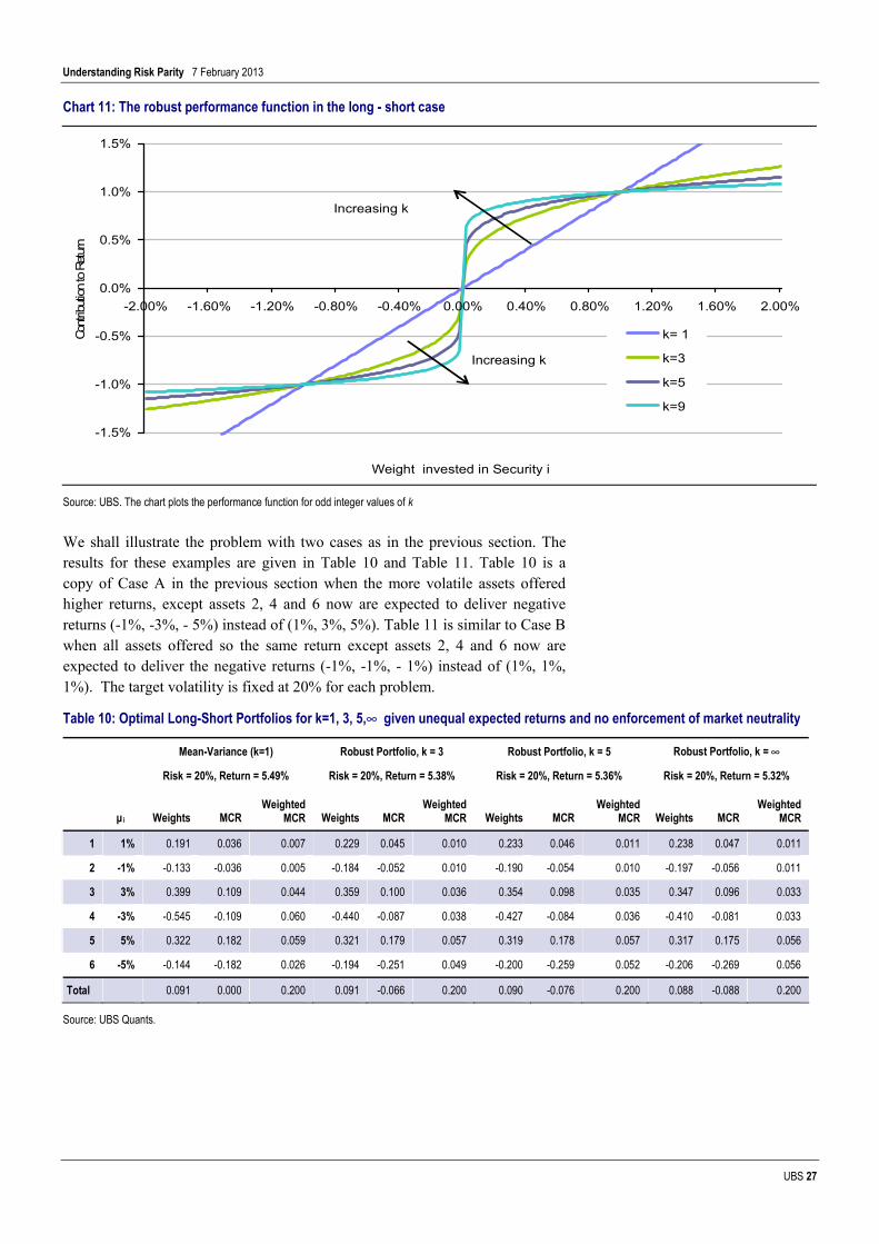
Again this is very similar to the standard problem except we have introduced diminishing marginal returns to taking a large position in any asset. On the long side, the argument is identical to the long only case. On the short side, the arguments are just mirrored. As you take a larger and larger negative position, the marginal return decreases as the performance measure is symmetric around 0, see the figure below.


UBS 27

Chart 11: The robust performance function in the long - short case

-1.5%

-1.0%

-0.5%

0.0%

0.5%

1.0%

1.5%

-2.00% -1.60% -1.20% -0.80% -0.40% 0.00% 0.40% 0.80% 1.20% 1.60% 2.00%

Weight invested in Security i

Contr

ibutio

n to R

eturn

k= 1

k=3

k=5

k=9

Increasing k

Increasing k

Source: UBS. The chart plots the performance function for odd integer values of k

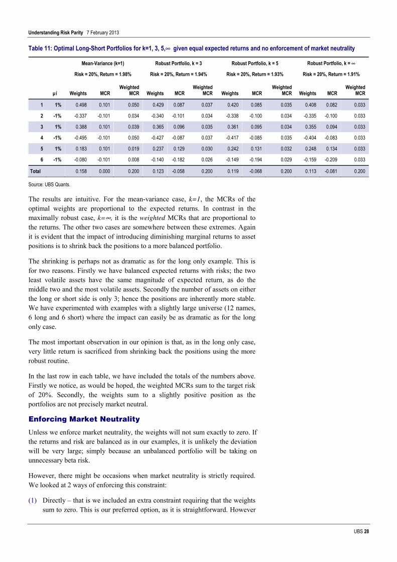
We shall illustrate the problem with two cases as in the previous section. The results for these examples are given in Table 10 and Table 11. Table 10 is a copy of Case A in the previous section when the more volatile assets offered higher returns, except assets 2, 4 and 6 now are expected to deliver negative returns (-1%, -3%, - 5%) instead of (1%, 3%, 5%). Table 11 is similar to Case B when all assets offered so the same return except assets 2, 4 and 6 now are expected to deliver the negative returns (-1%, -1%, - 1%) instead of (1%, 1%, 1%). The target volatility is fixed at 20% for each problem.

Table 10: Optimal Long-Short Portfolios for k=1, 3, 5,∞ given unequal expected returns and no enforcement of market neutrality


Risk = 20%, Return = 5.49% Risk = 20%, Return = 5.38% Risk = 20%, Return = 5.36% Risk = 20%, Return = 5.32%

µi Weights MCR Weighted




MCR

1 1% 0.191 0.036 0.007 0.229 0.045 0.010 0.233 0.046 0.011 0.238 0.047 0.011

2 -1% -0.133 -0.036 0.005 -0.184 -0.052 0.010 -0.190 -0.054 0.010 -0.197 -0.056 0.011

3 3% 0.399 0.109 0.044 0.359 0.100 0.036 0.354 0.098 0.035 0.347 0.096 0.033

4 -3% -0.545 -0.109 0.060 -0.440 -0.087 0.038 -0.427 -0.084 0.036 -0.410 -0.081 0.033

5 5% 0.322 0.182 0.059 0.321 0.179 0.057 0.319 0.178 0.057 0.317 0.175 0.056

6 -5% -0.144 -0.182 0.026 -0.194 -0.251 0.049 -0.200 -0.259 0.052 -0.206 -0.269 0.056

Total 0.091 0.000 0.200 0.091 -0.066 0.200 0.090 -0.076 0.200 0.088 -0.088 0.200

Source: UBS Quants.


UBS 28

Table 11: Optimal Long-Short Portfolios for k=1, 3, 5,∞ given equal expected returns and no enforcement of market neutrality







MCR

1 1% 0.498 0.101 0.050 0.429 0.087 0.037 0.420 0.085 0.035 0.408 0.082 0.033

2 -1% -0.337 -0.101 0.034 -0.340 -0.101 0.034 -0.338 -0.100 0.034 -0.335 -0.100 0.033

3 1% 0.388 0.101 0.039 0.365 0.096 0.035 0.361 0.095 0.034 0.355 0.094 0.033

4 -1% -0.495 -0.101 0.050 -0.427 -0.087 0.037 -0.417 -0.085 0.035 -0.404 -0.083 0.033

5 1% 0.183 0.101 0.019 0.237 0.129 0.030 0.242 0.131 0.032 0.248 0.134 0.033

6 -1% -0.080 -0.101 0.008 -0.140 -0.182 0.026 -0.149 -0.194 0.029 -0.159 -0.209 0.033

Total 0.158 0.000 0.200 0.123 -0.058 0.200 0.119 -0.068 0.200 0.113 -0.081 0.200

Source: UBS Quants.

The results are intuitive. For the mean-variance case, k=1, the MCRs of the optimal weights are proportional to the expected returns. In contrast in the maximally robust case, k=∞, it is the weighted MCRs that are proportional to the returns. The other two cases are somewhere between these extremes. Again it is evident that the impact of introducing diminishing marginal returns to asset positions is to shrink back the positions to a more balanced portfolio.

The shrinking is perhaps not as dramatic as for the long only example. This is for two reasons. Firstly we have balanced expected returns with risks; the two least volatile assets have the same magnitude of expected return, as do the middle two and the most volatile assets. Secondly the number of assets on either the long or short side is only 3; hence the positions are inherently more stable. We have experimented with examples with a slightly large universe (12 names, 6 long and 6 short) where the impact can easily be as dramatic as for the long only case.

The most important observation in our opinion is that, as in the long only case, very little return is sacrificed from shrinking back the positions using the more robust routine.

In the last row in each table, we have included the totals of the numbers above. Firstly we notice, as would be hoped, the weighted MCRs sum to the target risk of 20%. Secondly, the weights sum to a slightly positive position as the portfolios are not precisely market neutral.

Enforcing Market Neutrality

Unless we enforce market neutrality, the weights will not sum exactly to zero. If the returns and risk are balanced as in our examples, it is unlikely the deviation will be very large; simply because an unbalanced portfolio will be taking on unnecessary beta risk.

However, there might be occasions when market neutrality is strictly required. We looked at 2 ways of enforcing this constraint:

(1) Directly – that is we included an extra constraint requiring that the weights sum to zero. This is our preferred option, as it is straightforward. However


UBS 29

we lose the property that the weighted MCRs are proportional to the expected returns in the maximally robust case.

(2) Indirectly –we scale the expected returns on the short side up to induce the optimizer to take larger positions until the constraint is satisfied. Remember in this example, the optimiser preferred being slightly long. This approach had the advantage of preserving the property that weighted MCRs are proportional to the expected returns. Its disadvantage is that the scaling factor had to be estimated using an iterative search procedure.

We show the results of using these two different procedures in Table 12 and Table 13 below just for our case A (when returns vary across assets). Case B is has the same properties. Perhaps surprisingly, the final portfolio weights look very similar whichever approach is used. However, the adjustment in positions is slightly less using the first and simpler approach. This is because it puts fewer constraints on how the weights can be adjusted in order to achieve neutrality than the second approach (which effectively searches in 1 direction only).

Table 12: Optimal Long-Short Portfolios for k=1, 3, 5,∞ given unequal expected returns and direct enforcement of market neutrality







MCR

1 1% 0.141 0.016 0.002 0.190 0.025 0.005 0.196 0.026 0.005 0.203 0.028 0.006

2 -1% -0.162 -0.057 0.009 -0.210 -0.073 0.015 -0.215 -0.075 0.016 -0.221 -0.077 0.017

3 3% 0.388 0.089 0.035 0.345 0.077 0.027 0.340 0.075 0.026 0.333 0.073 0.024

4 -3% -0.549 -0.130 0.072 -0.450 -0.112 0.050 -0.438 -0.109 0.048 -0.422 -0.106 0.045

5 5% 0.326 0.163 0.053 0.320 0.154 0.049 0.318 0.152 0.048 0.315 0.150 0.047

6 -5% -0.143 -0.204 0.029 -0.194 -0.276 0.054 -0.200 -0.285 0.057 -0.207 -0.295 0.061

Total 0.000 -0.124 0.200 0.000 -0.205 0.200 0.000 -0.215 0.200 0.000 -0.228 0.200

Source: UBS Quants.

Table 13: Optimal Long-Short Portfolios for k=1, 3, 5,∞ given unequal expected returns & indirect enforcement of market neutrality







MCR

1 1% 0.236 0.019 0.005 0.233 0.027 0.006 0.234 0.028 0.006 0.235 0.029 0.007

2 -2.3% -0.086 -0.055 0.005 -0.181 -0.074 0.013 -0.189 -0.076 0.014 -0.199 -0.078 0.015

3 3% 0.353 0.057 0.020 0.333 0.063 0.021 0.329 0.063 0.021 0.323 0.062 0.020

4 -6.9% -0.591 -0.165 0.098 -0.445 -0.122 0.054 -0.430 -0.118 0.051 -0.411 -0.113 0.047

5 5% 0.261 0.096 0.025 0.281 0.118 0.033 0.281 0.119 0.033 0.281 0.119 0.034

6 -11.5% -0.174 -0.275 0.048 -0.220 -0.326 0.072 -0.225 -0.331 0.074 -0.230 -0.337 0.077

Total 0.000 -0.323 0.200 0.000 -0.314 0.200 0.000 -0.316 0.200 0.000 -0.318 0.200

Source: UBS Quants.


UBS 30

Appendix: generating return forecasts with a given IC We wish to generate a set of random forecasts of return with a given expected IC. If we take the vector of true returns as ȝ and the vector of forecast returns as r then we want

ICCorE =)),(( rȝ

Let us assume that

İȝr )1( kk −+=

where the İ are randomly distributed as N(0, ĳ2). Given there are two unknowns: k and ĳ then we need another equation to specify them both, so we choose

)()( ȝr VarVar =

where the variances are cross sectional.

Some algebra gets us to the result that k = IC and

2

22

)1()1(*)(

ICICVar

−−= µϕ


UBS 31

References Allen, Gregory (2010), ‘The Risk Parity Approach to Asset Allocation,’ Callan Investments Institute, Callan Associates, February.

Almgren, R., Thum, C., Hauptmann, E., & Li, H. (2005). Direct estimation of equity market impact. Risk, 18(7), 58-62.

Anderson, R.M., S.W. Bianchi and L.R. Goldberg (2012) Will my risk parity strategy outperform? Available at SSRN: http://ssrn.com/abstract=2101898 or http://dx.doi.org/10.2139/ssrn.2101898

Asness, C., Frazzini, A., & Pedersen, L. H. (2012). Leverage Aversion and Risk Parity. Financial Analysts Journal, 68(1), 47-59.

Bekaert, G., & Liu, J. (2004). Conditioning information and variance bounds on pricing kernels. Review of Financial Studies, 17(2), 339-378.

Broadie, M. (1993) Computing efficient frontiers using estimated parameters Annals of Operations Research, Vol 45, Issue 1, pp 21-58.

Carroll, Raymond J., (1989). Redescending M-Estimators; in Encyclopedia of Statistical Sciences, Supplement Volume, pp. 134-137 (John Wiley, New York).

Ferson, W. E., & Siegel, A. F. (2003). Stochastic discount factor bounds with conditioning information. Review of Financial Studies, 16(2), 567-595.

Ferson, W. E., & Siegel, A. F. (2001). ‘The efficient use of conditioning information in portfolios’, The Journal of Finance, 56(3), 967-982.

Foresti, Steven, and Michael Rush (2010), “Risk-Focused Diversification: Utilizing Leverage within Asset Allocation,” Wilshire Consulting, February 11, 2010.

Hampel, Frank R., (1974). The influence curve and its role in robust estimation, Journal of the American Statistical Association, 69, 383-393.

Inker, Ben (2010). ‘The Hidden Risk of Risk Parity Portfolios’, GMO White Paper, March 2010.

Lee, Wai (2011). "Risk-Based Asset Allocation: A New Answer to an Old Question?", The Journal of Portfolio Management 37(4), 11-28.

Kissell, R. (2008). Transaction Cost Analysis. The Journal of Trading, 3(2), 29-37.

Kritzman, M. (2006). Are Optimizers Error Maximizers? The Journal of Portfolio Management, 32(4), 66-69.

Teiletche, J., Roncalli, T., & Maillard, S. (2010). The properties of equally-weighted risk contributions portfolios. Journal of Portfolio Management, 36(4), 60.

O’Gorman, Aongus (2012). Risk Parity and Portfolio Construction, Round Tower Perspectives, August 2012.

http://dx.doi.org/10.2139/ssrn.2101898


UBS 32

Q Analyst Certification

Each research analyst primarily responsible for the content of this research report, in whole or in part, certifies that with respect to each security or issuer that the analyst covered in this report: (1) all of the views expressed accurately reflect his or her personal views about those securities or issuers and were prepared in an independent manner, including with respect to UBS, and (2) no part of his or her compensation was, is, or will be, directly or indirectly, related to the specific recommendations or views expressed by that research analyst in the research report.


UBS 33

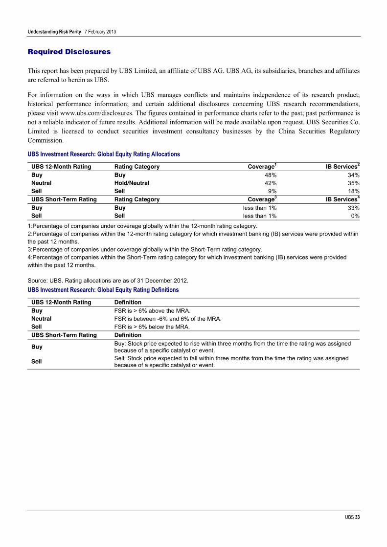
Required Disclosures This report has been prepared by UBS Limited, an affiliate of UBS AG. UBS AG, its subsidiaries, branches and affiliates are referred to herein as UBS.

For information on the ways in which UBS manages conflicts and maintains independence of its research product; historical performance information; and certain additional disclosures concerning UBS research recommendations, please visit www.ubs.com/disclosures. The figures contained in performance charts refer to the past; past performance is not a reliable indicator of future results. Additional information will be made available upon request. UBS Securities Co. Limited is licensed to conduct securities investment consultancy businesses by the China Securities Regulatory Commission.

UBS Investment Research: Global Equity Rating Allocations

UBS 12-Month Rating Rating Category Coverage1 IB Services2

Buy Buy 48% 34%Neutral Hold/Neutral 42% 35%Sell Sell 9% 18%UBS Short-Term Rating Rating Category Coverage3 IB Services4

Buy Buy less than 1% 33%Sell Sell less than 1% 0%

1:Percentage of companies under coverage globally within the 12-month rating category. 2:Percentage of companies within the 12-month rating category for which investment banking (IB) services were provided within the past 12 months. 3:Percentage of companies under coverage globally within the Short-Term rating category. 4:Percentage of companies within the Short-Term rating category for which investment banking (IB) services were provided within the past 12 months. Source: UBS. Rating allocations are as of 31 December 2012. UBS Investment Research: Global Equity Rating Definitions

UBS 12-Month Rating Definition Buy FSR is > 6% above the MRA. Neutral FSR is between -6% and 6% of the MRA. Sell FSR is > 6% below the MRA. UBS Short-Term Rating Definition

Buy Buy: Stock price expected to rise within three months from the time the rating was assigned because of a specific catalyst or event.

Sell Sell: Stock price expected to fall within three months from the time the rating was assigned because of a specific catalyst or event.


UBS 34

KEY DEFINITIONS Forecast Stock Return (FSR) is defined as expected percentage price appreciation plus gross dividend yield over the next 12 months. Market Return Assumption (MRA) is defined as the one-year local market interest rate plus 5% (a proxy for, and not a forecast of, the equity risk premium). Under Review (UR) Stocks may be flagged as UR by the analyst, indicating that the stock's price target and/or rating are subject to possible change in the near term, usually in response to an event that may affect the investment case or valuation. Short-Term Ratings reflect the expected near-term (up to three months) performance of the stock and do not reflect any change in the fundamental view or investment case. Equity Price Targets have an investment horizon of 12 months. EXCEPTIONS AND SPECIAL CASES UK and European Investment Fund ratings and definitions are: Buy: Positive on factors such as structure, management, performance record, discount; Neutral: Neutral on factors such as structure, management, performance record, discount; Sell: Negative on factors such as structure, management, performance record, discount. Core Banding Exceptions (CBE): Exceptions to the standard +/-6% bands may be granted by the Investment Review Committee (IRC). Factors considered by the IRC include the stock's volatility and the credit spread of the respective company's debt. As a result, stocks deemed to be very high or low risk may be subject to higher or lower bands as they relate to the rating. When such exceptions apply, they will be identified in the Company Disclosures table in the relevant research piece. Research analysts contributing to this report who are employed by any non-US affiliate of UBS Securities LLC are not registered/qualified as research analysts with the NASD and NYSE and therefore are not subject to the restrictions contained in the NASD and NYSE rules on communications with a subject company, public appearances, and trading securities held by a research analyst account. The name of each affiliate and analyst employed by that affiliate contributing to this report, if any, follows. UBS Limited: David Jessop; Claire Jones, CFA; Simon Stoye; Heran Zhang. UBS Securities LLC: Sebastian Lancetti, CFA. UBS Securities Asia Limited: Kenneth Tan. UBS Securities Australia Ltd: Paul Winter. Unless otherwise indicated, please refer to the Valuation and Risk sections within the body of this report.


UBS 35

Global Disclaimer This document has been prepared by UBS Limited, an affiliate of UBS AG. UBS AG, its subsidiaries, branches and affiliates are referred to herein as UBS. This document is for distribution only as may be permitted by law. It is not directed to, or intended for distribution to or use by, any person or entity who is a citizen or resident of or located in any locality, state, country or other jurisdiction where such distribution, publication, availability or use would be contrary to law or regulation or would subject UBS to any registration or licensing requirement within such jurisdiction. It is published solely for information purposes; it is not an advertisement nor is it a solicitation or an offer to buy or sell any financial instruments or to participate in any particular trading strategy. No representation or warranty, either express or implied, is provided in relation to the accuracy, completeness or reliability of the information contained in this document (‘the Information’), except with respect to Information concerning UBS. The Information is not intended to be a complete statement or summary of the securities, markets or developments referred to in the document. UBS does not undertake to update or keep current the Information. Any opinions expressed in this document may change without notice and may differ or be contrary to opinions expressed by other business areas or groups of UBS. Nothing in this document constitutes a representation that any investment strategy or recommendation is suitable or appropriate to an investor’s individual circumstances or otherwise constitutes a personal recommendation. Investments involve risks, and investors should exercise prudence and their own judgement in making their investment decisions. The financial instruments described in the document may not be eligible for sale in all jurisdictions or to certain categories of investors. Options, derivative products and futures are not suitable for all investors, and trading in these instruments is considered risky. Mortgage and asset-backed securities may involve a high degree of risk and may be highly volatile in response to fluctuations in interest rates or other market conditions. Foreign currency rates of exchange may adversely affect the value, price or income of any security or related instrument referred to in the document. For investment advice, trade execution or other enquiries, clients should contact their local sales representative. The value of any investment or income may go down as well as up, and investors may not get back the full amount invested. Past performance is not necessarily a guide to future performance. Neither UBS nor any of its directors, employees or agents accepts any liability for any loss (including investment loss) or damage arising out of the use of all or any of the Information. Any prices stated in this document are for information purposes only and do not represent valuations for individual securities or other financial instruments. There is no representation that any transaction can or could have been effected at those prices, and any prices do not necessarily reflect UBS's internal books and records or theoretical model-based valuations and may be based on certain assumptions. Different assumptions by UBS or any other source may yield substantially different results. Research will initiate, update and cease coverage solely at the discretion of UBS Investment Bank Research Management. The analysis contained in this document is based on numerous assumptions. Different assumptions could result in materially different results. The analyst(s) responsible for the preparation of this document may interact with trading desk personnel, sales personnel and other parties for the purpose of gathering, applying and interpreting market information. UBS relies on information barriers to control the flow of information contained in one or more areas within UBS into other areas, units, groups or affiliates of UBS. The compensation of the analyst who prepared this document is determined exclusively by research management and senior management (not including investment banking). Analyst compensation is not based on investment banking revenues; however, compensation may relate to the revenues of UBS Investment Bank as a whole, of which investment banking, sales and trading are a part. For financial instruments admitted to trading on an EU regulated market: UBS AG, its affiliates or subsidiaries (excluding UBS Securities LLC) acts as a market maker or liquidity provider (in accordance with the interpretation of these terms in the UK) in the financial instruments of the issuer save that where the activity of liquidity provider is carried out in accordance with the definition given to it by the laws and regulations of any other EU jurisdictions, such information is separately disclosed in this document. For financial instruments admitted to trading on a non-EU regulated market: UBS may act as a market maker save that where this activity is carried out in the US in accordance with the definition given to it by the relevant laws and regulations, such activity will be specifically disclosed in this document. UBS may have issued a warrant the value of which is based on one or more of the financial instruments referred to in the document. UBS and its affiliates and employees may have long or short positions, trade as principal and buy and sell in instruments or derivatives identified herein; such transactions or positions may be inconsistent with the opinions expressed in this document.


UBS 36

United Kingdom and the rest of Europe: Except as otherwise specified herein, this material is distributed by UBS Limited to persons who are eligible counterparties or professional clients. UBS Limited is authorised and regulated by the Financial Services Authority (FSA). France: Prepared by UBS Limited and distributed by UBS Limited and UBS Securities France S.A. UBS Securities France S.A. is regulated by the Autorité des Marchés Financiers (AMF). Where an analyst of UBS Securities France S.A. has contributed to this document, the document is also deemed to have been prepared by UBS Securities France S.A. Germany: Prepared by UBS Limited and distributed by UBS Limited and UBS Deutschland AG. UBS Deutschland AG is regulated by the Bundesanstalt fur Finanzdienstleistungsaufsicht (BaFin). Spain: Prepared by UBS Limited and distributed by UBS Limited and UBS Securities España SV, SA. UBS Securities España SV, SA is regulated by the Comisión Nacional del Mercado de Valores (CNMV). Turkey: Prepared by UBS Menkul Degerler AS on behalf of and distributed by UBS Limited. No information in this document is provided for the purpose of offering, marketing and sale by any means of any capital market instruments and services in the Republic of Turkey. Therefore, this document may not be considered as an offer made or to be made to residents of the Republic of Turkey. UBS AG is not licensed by the Turkish Capital Market Board under the provisions of the Capital Market Law (Law No. 2499). Accordingly, neither this document nor any other offering material related to the instruments/services may be utilized in connection with providing any capital market services to persons within the Republic of Turkey without the prior approval of the Capital Market Board. However, according to article 15 (d) (ii) of the Decree No. 32, there is no restriction on the purchase or sale of the securities abroad by residents of the Republic of Turkey. Poland: Distributed by UBS Limited (spolka z ograniczona odpowiedzialnoscia) Oddzial w Polsce. Russia: Prepared and distributed by UBS Securities CJSC. Switzerland: Distributed by UBS AG to persons who are institutional investors only. Italy: Prepared by UBS Limited and distributed by UBS Limited and UBS Italia Sim S.p.A. UBS Italia Sim S.p.A. is regulated by the Bank of Italy and by the Commissione Nazionale per le Società e la Borsa (CONSOB). Where an analyst of UBS Italia Sim S.p.A. has contributed to this document, the document is also deemed to have been prepared by UBS Italia Sim S.p.A. South Africa: Distributed by UBS South Africa (Pty) Limited, an authorised user of the JSE and an authorised Financial Services Provider. Israel: UBS Limited and its affiliates incorporated outside Israel are not licensed under the Investment Advice Law. This material is being issued only to and/or is directed only at persons who are Sophisticated Investors within the meaning of the Israeli Securities Law, and this material must not be relied or acted upon by any other persons. Whilst UBS Limited holds insurance for its activities, it does not hold the same insurance that would be required for an investment advisor or investment marketer under the relevant Investment Advice Law Regulations. Saudi Arabia: This document has been issued by UBS AG (and/or any of its subsidiaries, branches or affiliates), a public company limited by shares, incorporated in Switzerland with its registered offices at Aeschenvorstadt 1, CH-4051 Basel and Bahnhofstrasse 45, CH-8001 Zurich. This publication has been approved by UBS Saudi Arabia (a subsidiary of UBS AG), a foreign closed joint stock company incorporated in the Kingdom of Saudi Arabia under commercial register number 1010257812 having its registered office at Tatweer Towers, P.O. Box 75724, Riyadh 11588, Kingdom of Saudi Arabia. UBS Saudi Arabia is authorized and regulated by the Capital Market Authority to conduct securities business under license number 08113-37. United States: Distributed to US persons by either UBS Securities LLC or by UBS Financial Services Inc., subsidiaries of UBS AG; or by a group, subsidiary or affiliate of UBS AG that is not registered as a US broker-dealer (a ‘non-US affiliate’) to major US institutional investors only. UBS Securities LLC or UBS Financial Services Inc. accepts responsibility for the content of a document prepared by another non-US affiliate when distributed to US persons by UBS Securities LLC or UBS Financial Services Inc. All transactions by a US person in the securities mentioned in this document must be effected through UBS Securities LLC or UBS Financial Services Inc., and not through a non-US affiliate. Canada: Distributed by UBS Securities Canada Inc., a registered investment dealer in Canada and a Member-Canadian Investor Protection Fund, or by another affiliate of UBS AG that is registered to conduct business in Canada or is otherwise exempt from registration. Hong Kong: Distributed by UBS Securities Asia Limited. Singapore: Distributed by UBS Securities Pte. Ltd. [mica (p) 016/11/2011 and Co. Reg. No.: 198500648C] or UBS AG, Singapore Branch. Please contact UBS Securities Pte. Ltd., an exempt financial adviser under the Singapore Financial Advisers Act (Cap. 110); or UBS AG, Singapore Branch, an exempt financial adviser under the Singapore Financial Advisers Act (Cap. 110) and a wholesale bank licensed under the Singapore Banking Act (Cap. 19) regulated by the Monetary Authority of Singapore, in respect of any matters arising from, or in connection with, the analysis or document. The recipients of this document represent and warrant that they are accredited and institutional investors as defined in the Securities and Futures Act (Cap. 289). Japan: Distributed by UBS Securities Japan Co., Ltd. to institutional investors only. Where this document has been prepared by UBS Securities Japan Co., Ltd., UBS Securities Japan Co., Ltd. is the author, publisher and distributor of the document. Australia: Distributed by UBS AG (Holder of Australian Financial Services License No. 231087) and/or UBS Securities Australia Ltd (Holder of Australian Financial Services License No. 231098). The Information in this document has been prepared without taking into account any investor’s objectives, financial situation or needs, and investors should, before acting on the Information, consider the appropriateness of the Information, having regard to their objectives, financial situation and needs. If the Information contained in this document relates to the acquisition, or potential acquisition of a particular financial product by a ‘Retail’ client as defined by section 761G of the Corporations Act 2001 where a Product Disclosure Statement would be required, the retail client should obtain and consider the Product Disclosure Statement relating to the product before making any decision about whether to acquire the product. New Zealand: Distributed by UBS New Zealand Ltd. The information and recommendations in this publication are provided for general information purposes only. To the extent that any such information or recommendations constitute financial advice, they do not take into account any person’s particular financial situation or goals. We recommend that recipients seek advice specific to their circumstances from their financial advisor. Dubai: The research prepared and distributed by UBS AG Dubai Branch is intended for Professional Clients only and is not for further distribution within the United Arab Emirates. Korea: Distributed in Korea by UBS Securities Pte. Ltd., Seoul Branch. This document may have been edited or contributed to from time to time by affiliates of UBS Securities Pte. Ltd., Seoul Branch. Malaysia: This material is authorized to be distributed in Malaysia by UBS Securities Malaysia Sdn. Bhd (253825-x). India: Prepared by UBS Securities India Private Ltd. 2/F, 2 North Avenue, Maker Maxity, Bandra Kurla Complex, Bandra (East), Mumbai (India) 400051. Phone: +912261556000 SEBI Registration Numbers: NSE (Capital Market Segment): INB230951431, NSE (F&O Segment) INF230951431, BSE (Capital Market Segment) INB010951437. The disclosures contained in research documents produced by UBS Limited shall be governed by and construed in accordance with English law. UBS specifically prohibits the redistribution of this document in whole or in part without the written permission of UBS and UBS accepts no liability whatsoever for the actions of third parties in this respect. Images may depict objects or elements which are protected by third party copyright, trademarks and other intellectual property rights. © UBS 2013. The key symbol and UBS are among the registered and unregistered trademarks of UBS. All rights reserved.

��

Sefton Jessop - Getting Performance Out of Risk Parity

Documents

Transcript of Sefton Jessop - Getting Performance Out of Risk Parity