SECURE BIOMETRIC COMPUTATION AND …fbayatba/Publications/Thesis-phd.pdfSECURE BIOMETRIC COMPUTATION...

SECURE BIOMETRIC COMPUTATION AND OUTSOURCING

A Dissertation

Submitted to the Graduate School

of the University of Notre Dame

in Partial Fulfillment of the Requirements

for the Degree of

Doctor of Philosophy

by

Fattaneh Bayatbabolghani

Marina Blanton, Co-Director

Aaron Striegel, Co-Director

Graduate Program in Computer Science and Engineering

Notre Dame, Indiana

June 2017

SECURE BIOMETRIC COMPUTATION AND OUTSOURCING

Abstract

by


Biometric computations are becoming increasingly popular, and their impact in

real world applications is undeniable. There are di↵erent types of biometric data used

in a variety of applications such as biometric recognition including verification and

identification. Because of the highly sensitive nature of biometric data, its protection

is essential during biometric computations.

Based on the computations that need to be carried out and the type of biometric

data, there is a need for application-specific privacy preserving solutions. These so-

lutions can be provided by developing secure biometric computations in a way that

no information gets revealed during the protocol execution. In some biometric ap-

plications (e.g. verification and identification), data is distributed amongst di↵erent

parties engaged in computations. In some other applications, the execution of com-

putations is bounded by the computational power of the parties, motivating the use

of cloud or external servers. In both these cases, 1) there is a higher risk for sensitive

data to be disclosed, making secure biometric protocols a prominent need for such

practical applications, 2) it is more challenging to develop novel and e�cient solutions

for these computational settings, making the design of secure biometric protocols a

research-worthy e↵ort.


In our research, we worked on three di↵erent biometric modalities which require

various computational settings. In more detail:

• We focused on voice recognition in semi-honest and malicious adversarial mod-els using floating point arithmetic (the most common and accurate type ofdata for voice recognition). Based on the application, we considered two securecomputational settings which are two-party and multi-party settings. For thispurpose, we designed new secure floating-point operations necessary for voicerecognition computations.

• We designed novel and general approaches to securely compute three genomictests (i.e., paternity, ancestry, and genomic compatibility). We consideredserver aided two-party computation for those applications. Also, based on thegenomic computational settings we proposed novel certified inputs technique toprovide stronger security guarantees with respect to malicious users.

• We built secure fingerprint recognition protocols which include both alignment(for the first time) and matching processes. The solutions were proposed in bothtwo-party and multi-party computational settings. We also designed a num-ber of new secure and e�cient protocols for essential operations in fingerprintrecognition process.

To the best of our knowledge, our unique contributions in di↵erent biometric

modalities largely benefit the field of secure biometric computation. Our solutions

consider the nature of computational setting (two-party and multi-party settings) of

biometric applications in practice, and e�ciently protect the data during the com-

putations. In addition, our secure protocols and building blocks are general and can

be used for other applications where the same data types and settings are used.

CONTENTS

FIGURES . . . . . . . . . . . . . . . . . . . . . . . . . . . . . . . . . . . . . . vi

TABLES . . . . . . . . . . . . . . . . . . . . . . . . . . . . . . . . . . . . . . vii

ACKNOWLEDGMENTS . . . . . . . . . . . . . . . . . . . . . . . . . . . . . viii

CHAPTER 1: INTRODUCTION . . . . . . . . . . . . . . . . . . . . . . . . . 11.1 Voice Recognition . . . . . . . . . . . . . . . . . . . . . . . . . . . . . 31.2 DNA Computation . . . . . . . . . . . . . . . . . . . . . . . . . . . . 41.3 Fingerprint Recognition . . . . . . . . . . . . . . . . . . . . . . . . . 51.4 Organization . . . . . . . . . . . . . . . . . . . . . . . . . . . . . . . 6

CHAPTER 2: RELATED WORK . . . . . . . . . . . . . . . . . . . . . . . . 72.1 Related Work in Secure Voice Recognition . . . . . . . . . . . . . . . 72.2 Related Work in Secure DNA Computation . . . . . . . . . . . . . . 92.3 Related Work in Secure Fingerprint Recognition . . . . . . . . . . . . 11

CHAPTER 3: PRELIMINARIES . . . . . . . . . . . . . . . . . . . . . . . . . 133.1 Secure Two-Party and Multi-Party Computational Techniques . . . . 13

3.1.1 Homomorphic Encryption . . . . . . . . . . . . . . . . . . . . 133.1.2 Secret Sharing . . . . . . . . . . . . . . . . . . . . . . . . . . . 143.1.3 Garbled Circuit Evaluation . . . . . . . . . . . . . . . . . . . 16

3.2 Secure Building Blocks . . . . . . . . . . . . . . . . . . . . . . . . . . 173.2.1 Fixed-Point and Integer Building Blocks . . . . . . . . . . . . 183.2.2 Floating-Point Building Blocks . . . . . . . . . . . . . . . . . 22

3.3 Signature and Commitment Schemes . . . . . . . . . . . . . . . . . . 233.4 Zero-Knowledge Proofs of Knowledge . . . . . . . . . . . . . . . . . . 263.5 Security Model . . . . . . . . . . . . . . . . . . . . . . . . . . . . . . 28

CHAPTER 4: VOICE RECOGNITIONS . . . . . . . . . . . . . . . . . . . . 314.1 Motivation . . . . . . . . . . . . . . . . . . . . . . . . . . . . . . . . . 324.2 Contributions . . . . . . . . . . . . . . . . . . . . . . . . . . . . . . . 334.3 Hidden Markov Models and Gaussian Mixture Models . . . . . . . . . 354.4 Framework . . . . . . . . . . . . . . . . . . . . . . . . . . . . . . . . . 36

4.4.1 Two-Party Computation . . . . . . . . . . . . . . . . . . . . . 37

iii

4.4.2 Multi-Party Computation . . . . . . . . . . . . . . . . . . . . 384.5 Secure HMM and GMM Computation in the Semi-Honest Model . . . 394.6 Secure HMM and GMM Computation in the Malicious Model . . . . 45

4.6.1 Multi-Party Setting . . . . . . . . . . . . . . . . . . . . . . . . 454.6.2 Two-Party Setting . . . . . . . . . . . . . . . . . . . . . . . . 46

4.6.2.1 Secure Multiplication . . . . . . . . . . . . . . . . . . 474.6.2.2 Secure Comparison . . . . . . . . . . . . . . . . . . . 494.6.2.3 Secure Truncation . . . . . . . . . . . . . . . . . . . 544.6.2.4 Secure Inversion . . . . . . . . . . . . . . . . . . . . 574.6.2.5 Secure Prefix Multiplication . . . . . . . . . . . . . . 594.6.2.6 Secure Bit Decomposition . . . . . . . . . . . . . . . 634.6.2.7 Performance of the New Building Blocks . . . . . . . 68

CHAPTER 5: DNA COMPUTATIONS . . . . . . . . . . . . . . . . . . . . . 705.1 Motivation . . . . . . . . . . . . . . . . . . . . . . . . . . . . . . . . . 705.2 Contributions . . . . . . . . . . . . . . . . . . . . . . . . . . . . . . . 715.3 Genomic Testing . . . . . . . . . . . . . . . . . . . . . . . . . . . . . 755.4 Security Model . . . . . . . . . . . . . . . . . . . . . . . . . . . . . . 785.5 Server-Aided Computation . . . . . . . . . . . . . . . . . . . . . . . . 81

5.5.1 Semi-Honest A and B, Malicious S . . . . . . . . . . . . . . . 815.5.2 Semi-Honest S, Malicious A and B . . . . . . . . . . . . . . . 855.5.3 Semi-Honest S, Malicious A and B with Input Certification . . 90

5.6 Private Genomic Computation . . . . . . . . . . . . . . . . . . . . . . 945.6.1 Ancestry Test . . . . . . . . . . . . . . . . . . . . . . . . . . . 965.6.2 Paternity Test . . . . . . . . . . . . . . . . . . . . . . . . . . . 965.6.3 Genetic Compatibility Test . . . . . . . . . . . . . . . . . . . 97

5.7 Performance Evaluation . . . . . . . . . . . . . . . . . . . . . . . . . 1005.7.1 Ancestry Test . . . . . . . . . . . . . . . . . . . . . . . . . . . 1015.7.2 Paternity Test . . . . . . . . . . . . . . . . . . . . . . . . . . . 1035.7.3 Genetic Compatibility Test . . . . . . . . . . . . . . . . . . . 106

CHAPTER 6: FINGERPRINT RECOGNITIONS . . . . . . . . . . . . . . . 1086.1 Motivation . . . . . . . . . . . . . . . . . . . . . . . . . . . . . . . . . 1096.2 Contributions . . . . . . . . . . . . . . . . . . . . . . . . . . . . . . . 1096.3 Fingerprint Background . . . . . . . . . . . . . . . . . . . . . . . . . 112

6.3.1 Fingerprint Recognition Using Brute Force Geometrical Trans-formation . . . . . . . . . . . . . . . . . . . . . . . . . . . . . 113

6.3.2 Fingerprint Recognition Using High Curvature Points for Align-ment . . . . . . . . . . . . . . . . . . . . . . . . . . . . . . . . 113

6.3.3 Fingerprint Recognition based on Spectral Minutiae Represen-tation . . . . . . . . . . . . . . . . . . . . . . . . . . . . . . . 118

6.4 Problem Statement . . . . . . . . . . . . . . . . . . . . . . . . . . . . 1216.5 Secure Building Blocks . . . . . . . . . . . . . . . . . . . . . . . . . . 122

6.5.1 New Building Blocks . . . . . . . . . . . . . . . . . . . . . . . 123

iv

6.5.1.1 Sine, Cosine, and Arctangent . . . . . . . . . . . . . 1236.5.1.2 Square Root . . . . . . . . . . . . . . . . . . . . . . 1326.5.1.3 Selection . . . . . . . . . . . . . . . . . . . . . . . . 135

6.6 Secure Fingerprint Recognition . . . . . . . . . . . . . . . . . . . . . 1396.6.1 Secure Fingerprint Recognition Using Brute Force Geometrical

Transformation . . . . . . . . . . . . . . . . . . . . . . . . . . 1406.6.2 Secure Fingerprint Recognition Using High Curvature Points

for Alignment . . . . . . . . . . . . . . . . . . . . . . . . . . . 1446.6.3 Secure Fingerprint Recognition based on Spectral Minutia Rep-

resentation . . . . . . . . . . . . . . . . . . . . . . . . . . . . . 1496.7 Performance Evaluation . . . . . . . . . . . . . . . . . . . . . . . . . 153

CHAPTER 7: CONCLUSIONS AND FUTURE DIRECTIONS . . . . . . . . 1567.1 Conclusions . . . . . . . . . . . . . . . . . . . . . . . . . . . . . . . . 156

7.1.1 Voice Recognition . . . . . . . . . . . . . . . . . . . . . . . . . 1567.1.2 DNA Computation . . . . . . . . . . . . . . . . . . . . . . . . 1577.1.3 Fingerprint Recognition . . . . . . . . . . . . . . . . . . . . . 157

7.2 Future Plan . . . . . . . . . . . . . . . . . . . . . . . . . . . . . . . . 1587.2.1 E�cient Input Certification Protocols . . . . . . . . . . . . . . 1587.2.2 Secure Protocols in the Presence of a Covert Adversary . . . . 1587.2.3 Data Mining Computations on Large-Scale Data Sets . . . . . 159

BIBLIOGRAPHY . . . . . . . . . . . . . . . . . . . . . . . . . . . . . . . . . 160

v

FIGURES

4.1 Performance of integer HMM’s building blocks in the homomorphicencryption setting. . . . . . . . . . . . . . . . . . . . . . . . . . . . . 41

4.2 Performance of floating-point HMM’s building blocks in the homomor-phic encryption setting. . . . . . . . . . . . . . . . . . . . . . . . . . . 42

4.3 Performance of HMM computation for varying N and T in the homo-morphic encryption setting. . . . . . . . . . . . . . . . . . . . . . . . 43

4.4 Performance of HMM computation for varying N and T in the secretsharing setting. . . . . . . . . . . . . . . . . . . . . . . . . . . . . . . 44

5.1 Illustration of Protocol 1 with weak A (who contributes only garbledlabels for her input wires to the computation). . . . . . . . . . . . . . 83

5.2 Illustration of Protocol 2. . . . . . . . . . . . . . . . . . . . . . . . . . 88

6.1 A set of minutiae with orientations. The image is generated by NIST’sFingeprint Minutiae Viewer (FpMV) software [7] using a fingerprintfrom NIST’s Special Database 4 [5]. . . . . . . . . . . . . . . . . . . . 110

vi

TABLES

3.1 PERFORMANCE OF KNOWN SECURE BUILDING BLOCKS ONINTEGER AND FIXED-POINT VALUES IN SECRET SHARING . 21

3.2 PERFORMANCE OF KNOWN SECURE BUILDING BLOCKS ONINTEGER AND FIXED-POINT VALUES IN GARBLED CIRCUIT 22

3.3 COMPLEXITY OF FLOATING-POINT PROTOCOLS IN SECRETSHARING . . . . . . . . . . . . . . . . . . . . . . . . . . . . . . . . . 24

3.4 COMPLEXITY OF FLOATING-POINT PROTOCOLS IN HOMO-MORPHIC ENCRYPTION . . . . . . . . . . . . . . . . . . . . . . . 25

3.5 COMPLEXITY OF ZKPKS IN HOMOMORPHIC ENCRYPTION . 27

4.1 COMPLEXITY OF BUILDING BLOCKS IN THE TWO-PARTYSETTING BASED ON HOMOMORPHIC ENCRYPTION . . . . . . 69

5.1 PERFORMANCEOF ANCESTRY TESTWITHOUT/WITH HALF-GATES . . . . . . . . . . . . . . . . . . . . . . . . . . . . . . . . . . 102

5.2 PERFORMANCEOF ANCESTRY TESTWITHOUT SERVERWITH-OUT/WITH HALF-GATES . . . . . . . . . . . . . . . . . . . . . . . 103

5.3 PERFORMANCE OF PATERNITY TEST (NO HALF-GATES) . . 104

5.4 PERFORMANCE OF COMPATIBILITY TEST (NO HALF-GATES) 106

6.1 PERFORMANCE OF PROPOSED SECURE BUILDING BLOCKSBASED ON SECRET SHARING FOR FIXED-POINT VALUES . . 129

6.2 PERFORMANCE OF PROPOSED SECURE BUILDING BLOCKSBASED ON GARBLED CIRCUIT FOR FIXED-POINT VALUES . 130

6.3 EXECUTION TIME OF PROTOCOL SpectralFR IN SECONDS US-ING THE SECRET SHARING . . . . . . . . . . . . . . . . . . . . . 154

6.4 EXECUTION TIME OF PROTOCOL SpectralFR IN SECONDS ANDTHE TOTAL NUMBER OF GATES (IN MILLIONS) IN ITS IMPLE-MENTATION USING THE GARBLED CIRCUIT . . . . . . . . . . 155

vii

ACKNOWLEDGMENTS

I would like to thank so many people for helping me during this journey. They

made my last four years a lot easier that I thought it was going to be. I am truly

appreciative for their support.

I would like to genuinely thank my advisor, Prof. Marina Blanton. I learned many

lessons from her, from foundations of scientific research, to being a hard-working,

motivated, passionate, and professional researcher. I also learned from her to be

much more open to discussions and to take into account di↵erent points of view

before proposing a new idea. I will always be grateful for the opportunity that I was

given to work under her advice.

In addition, I was privileged to work with Prof. Mehrdad Aliasgari, a knowledge-

able and inspiring researcher, in di↵erent research projects. I am really thankful for

all his support throughout my Ph.D. years, and his early guidance before starting

my work at Notre Dame.

I would like to deeply thank Prof. Aaron Striegel, Prof. Walter Scheirer, and

Prof. Scott Emrich for providing invaluable guidance and being always available to

help and support me during the last year of my Ph.D.

I also would like to thank the CSE family especially, Joyce Yeats and Ivor Zhang

among all. Joyce was truly helpful to me particularly in academic procedures, and

Ivor was a friendly collaborator and his ideas were always constructive in my research.

Moreover, I am thankful for having wonderful and supportive friends; they kept me

energetic and delighted during the last four years.

viii

Last but not least, I would like to acknowledge with support and love of my family-

My parents, Asgar and Ehteram; my husband, Kayhan; my brother and sister, Saeed

and Maryam. Without all their helps I doubt that I would reach up to this place

today.

ix

CHAPTER 1

INTRODUCTION

Biometric data is a type of data which comes from human characteristics such as

iris, voice, fingerprint, and DNA. Also, di↵erent types of biometric data have become

increasingly ubiquitous during recent decades. Because of the highly sensitive nature

of biometric data, protection is crucial in a variety of applications such as biometric

recognition for verification and identification.

Secure computation on biometric data is an emerging topic and it has been draw-

ing growing attention during recent years. There are di↵erent types of biometric data

with a variety of usages. Based on the type of biometric modality and its application,

we need to follow specific computations. These computations are usually carried out

on a large number of inputs, and it demands high computational power. Therefore,

optimizing the computations is necessary and makes this problem more challenging.

Also, oftentimes the data owner is computationally limited. Thus, outsourcing

the computations makes the solution more e�cient and more practical in real world

settings. However, assigning computations to the cloud or servers increases the risk

of revealing sensitive data. Thus, designing secure solutions for outsourced biometric

computations is even more challenging than the standard case.

Consequently, to address secure regular and outsourced biometric computations,

di↵erent computational settings are considered as follows:

• Two-party computation: Each party has his/her own inputs, and both are goingto jointly compute a function. Eventually, one party or both learn the outputdepending on the predefined settings and the utilized techniques.

1

• Server aided two-party computation: In some applications such as non-medicaluse of genomic data, computations often take place in a server-mediated settingwhere the server o↵ers the ability for joint computations between the users. Inthis setting, the two-party scenario is enhanced with a server which helps theparties to compute the function, while no information is being revealed to theserver.

• Multi-party computation: In this setting, usually one or two parties are going tooutsource data to a collection of outside parties to carry out computations col-lectively. The assumption here is the number of non-colluding parties is biggerthan a predetermined threshold; otherwise, the data can be compromised.

In addition to the computational settings introduced above, there are adversarial

models to be considered for the secure computations. Here, we consider two standard

adversarial models:

• Semi-honest or passive: This type of adversary is a party who correctly followsthe protocol specification, but it attempts to learn additional information byanalyzing the transcript of messages received during the execution.

• Malicious or active: This type of adversary is a party who can arbitrarilydeviate from the protocol specification.

Furthermore, each solution (based on the biometric modality and its usage) carries

out specific computations which contain some operations as building blocks. In addi-

tion, the structure of the building blocks may di↵er depending on the data type (i.e.,

integer, fixed point, and floating point), the secure computational setting, adversarial

model, and applied tools (e.g., garbled circuit and secret sharing). Therefore, this

demands some e↵ort to address all the security concerns and consider all varieties of

settings in biometric applications.

As a result of these research pursuits, one of the innovative contributions of our

work is the building of general and time-e�cient privacy-preserving solutions and

protocols which may be used not only with other biometric modalities, but also

in other types of computations where the privacy of the data is one of the main

concerns [12, 24, 31, 32, 109]. Furthermore, we worked on three common modalities

2

that have di↵erent real world applications: (1) Voice is utilized for speaker-based

authentication. (2) Genomic tests are used for a verity of purposes; for instance,

they help find common ancestors between two people (i.e., an ancestry test). (3)

Fingerprint is one of the most accurate types of biometric data for the purpose of

verification and identification. The following three sections will address these common

modalities in more detail.

1.1 Voice Recognition

Voice recognition includes speech recognition and speaker recognition. For both

tasks Hidden Markov Models (HMMs) are the most common and accurate approaches.

Thus, we concentrated on secure computation of HMMs. Furthermore, to ensure that

Gaussian mixture models (GMMs), which are commonly used in HMM computation,

can be a part of the secure computation, GMM computation is integrated into the

privacy-preserving solution.

In [12], we provided a privacy-preserving solution for the Viterbi decoding algo-

rithm (the most commonly used in voice recognition), but the techniques can be used

to securely execute other HMM decoding algorithms (e.g. the forward and the expec-

tation maximization algorithms) as well. In addition, we developed secure techniques

for computation with floating-point numbers, which provide adequate precision and

are the most appropriate for HMM computation. As a matter of fact, we developed

and implemented secure HMM computations in semi-honest model using floating

point numbers. The solution is also proven to have a reasonable performance.

From that point onward we continued to designed secure floating-point protocols

for necessary HMM operations (multiplication, comparison, truncation, inversion,

prefix multiplication, and bit decomposition) in stronger security circumstances for

the first time where the computational parties can arbitrarily deviate from the pro-

tocol specification (named as the malicious party). These protocols also have appli-

3

cability well beyond the HMM domain. Their rigorous simulation-based proofs of

security are constructed from scratch. They are the most challenging part of this

work, but constitute substantial contributions.

1.2 DNA Computation

During recent years the use of genomic data in a variety of applications has rapidly

expanded. It is especially important to protect genomic data because it can reveal

information not only about the data owner but also his/her relatives. Thus, this

portion of our research focused on general privacy-preserving protocols and solutions

which can be used for common DNA applications such as ancestry, paternity, and

genomic compatibility tests. These applications are normally facilitated by some

service provider or third party. Such service providers are as a point of contact for

aiding the individuals with private computations of their sensitive genomic data.

Therefore, it is more appropriate to assume that such computations are carried out

by two individuals through some third-party service provider.

Another important consideration from a security point of view is enforcing correct

(i.e., truthful) inputs to be entered into the computation. This requirement is outside

of the traditional security model and normally is not addressed, but it becomes

important in the context of genomic computation. This is because for certain types

of genomic tests it is easy for one participant to modify his inputs and learn sensitive

information about genetic conditions of the other party. For these reasons it is vital

that participants should be prevented from modifying their inputs used in genomic

computations.

In [31, 32], I studied private genomic computations in the light of server-mediated

or server-aided settings and utilized the server to lower the cost of the computations

for the participants. In addition, and also for the first time, stronger security guar-

antees with respect to malicious parties are provided. In particular, novel certified

4

inputs are incorporated into secure computations to guarantee that a malicious user

is unable to modify her inputs in order to learn information about the data of the

other user. The solutions are general in the sense that they can be used for other

computations and o↵er reasonable performance compared to the state of the art.

1.3 Fingerprint Recognition

Fingerprint recognition is an accurate method of identification. Fingerprints need

to be protected because they can reveal the identity of their owners. There are some

di↵erent techniques for fingerprint recognition, but most of them have two main

steps: the first step is alignment and the second one is matching. The purpose of

the alignment step is to improve the accuracy of the matching step. To the best of

our knowledge, all existing articles on secure fingerprint recognition focused on the

matching step because the alignment step is computationally expensive, albeit an

interesting challenge.

Therefore, we aimed to design an e�cient solution to the entire recognition process

including both the alignment and matching steps for the first time, in order to achieve

more reliable results [24]. We focused on three algorithms that compare fingerprints

using both alignment and matching. The algorithms are selected based on their

precision, speed, and/or popularity, with the goal of building e�cient and practical

security solutions.

The proposed solutions carry out specific computations, and they contain complex

operations that require dealing with non-integer values. As a result, a substantial

part of this work is dedicated to building practical and time-e�cient secure protocols

(sine, cosine, arctangent, square-root, and selecting the fth smallest element) for

non-integer operations.

5

1.4 Organization

In the rest of this dissertation: The related literature to this work is described

in Chapter 2. Chapter 3 provides all necessary cryptographic background and no-

tations. In Chapters 4–6, we describe our main contributions in terms of designing

secure, e�cient, and novel privacy-preserving protocols, and our proposed solutions

respectively for voice recognition, DNA computation, and fingerprint recognition.

And finally, at the end we discuss some conclusionary remarks and future directions

in Chapter 7.

6

CHAPTER 2

RELATED WORK

In this chapter, we are going to describe the related literature in secure biometric

computations. Firstly, we introduce previous voice recognition works in Section 2.1,

then we provide the recent works in the context of secure genomic computation

in Section 2.2. Finally, Section 2.3 is dedicated to explain related work in secure

fingerprint recognition.

2.1 Related Work in Secure Voice Recognition

To the best of our knowledge, privacy-preserving HMM computation was first con-

sidered in [113], which provides a secure two-party solution based on homomorphic

encryption for speech recognition using integer representation of values. In general,

integer representation is not su�cient for HMM computation because it involves var-

ious operations on probability values, which occupy a large range of real numbers and

demand high precision. In particular, probabilities need to be repeatedly multiplied

during HMM computation, and the resulting product can quickly diminish with each

multiplication, leading to inability to maintain precision using integer or fixed-point

representation. [113] computes this product using logarithms of the values, which

becomes the sum of logarithms (called logsum in [113]). This allows the solution

to retain some precision even with (scaled) integer representation, but the computa-

tion was nevertheless not shown to be computationally stable and the error was not

quantified. Also, as was mentioned in [60], one of the building blocks in [113] is not

secure.

7

The techniques of [113] were later used as-is in [111] for Gaussian mixture models.

The same idea was used in [104], [105] to develop privacy-preserving speaker veri-

fication for joint two-party computation, where the HMM parameters were stored

in an encrypted domain. Also, [106] treats speaker authentication and identifica-

tion and speech recognition in the same setting. Similar to [111], [103] aimed at

providing secure two-party GMM computation using the same high-level idea, but

with implementation di↵erences. The solution of [103], however, has security weak-

nesses. In particular, the protocol reveals a non-trivial amount of information about

the private inputs, which, in combination with other computation or outside knowl-

edge, may allow for full recovery of the inputs (additional detail about this security

weakness is provided in [10]). Some of the above techniques were also used in privacy-

preserving network analysis and anomaly detection in two-party or multi-party com-

putation [100, 101].

Another work [107] builds a privacy-preserving protocol for HMM computation in

the two-party setting using a third-party commodity server to aid the computation.

In [107], one participant owns the model and the other holds observations. We build

a more general solution that can be applied to both two-party (without an additional

server) and multi-party settings, uses high precision floating-point arithmetic, and is

secure in a stronger security setting (in the presence of malicious participants).

All of the above work uses integer-based representations, where in many cases

multiplications were replaced with additions of logarithms, as originated in [113].

With the exception of [106], these publications did not quantify the error, while us-

ing integer (or fixed-point) representation demands substantially larger bit length

representation than could be used otherwise and the error can accumulate and in-

troduce fatal inaccuracies. [106] evaluated the error and reports that it amounted to

0.52% for their specific set of parameters.

The need to use non-integer representation for HMM computation was recognized

8

in [61] and the authors proposed solutions for secure HMM forward algorithm com-

putation in the two-party setting using logarithmic representation of real numbers.

The solution that uses logarithmic representation was shown to be accurate for HMM

computation used in bioinformatics (see [60]), but it still has its limitations. In par-

ticular, the look-up tables used in [61] to implement certain operations in logarithmic

representations grow exponentially in the bitlength of the operands. This means that

the approach might not be suitable for some HMM applications or a set of param-

eters. The use of floating-point numbers, on the other hand, allows one to avoid

the di�culties mentioned above and provides a universal solution that works for any

application with a bounded (and controlled) error. Thus, we decided to address the

need to develop secure computation techniques for HMMs on standard real number

representations and provide the first provably secure floating-point solution for HMM

algorithms, which initially appeared in [10].

2.2 Related Work in Secure DNA Computation

There are a number of publications, e.g., [16, 18, 19] and others, that treat the

problem of privately computing personalized medicine tests with the goal of choosing

an optimal medical treatment or drug prescription. Ayday et al. [17] also focus

on privacy-preserving systems for storing genomic data by means of homomorphic

encryption.

To the best of our knowledge, privacy-preserving paternity testing was first con-

sidered by Bruekers et al. in [36]. The authors propose privacy-preserving protocols

for a number of genetic tests based on Short Tandem Repeats (STRs) (see Section

5.3 for detail). The tests include identity testing, paternity tests with one and two

parents, and common ancestry testing on the Y chromosome. The proposed proto-

cols for these tests are based on additively homomorphic public key encryption and

are secure in the presence of semi-honest participants. Implementation results were

9

not given in [36], but Baldi et al. [20] estimates that the paternity test in [36] is

several times slower than that in [20]. We thus compare our paternity test to the

performance of an equivalent test in [20].

Baldi et al. [20] concentrate on a di↵erent representation of genomic data (in

the form of fully-sequenced human genome) and provide solutions for paternity, drug

testing for personalized medicine, and genetic compatibility. The solutions use private

set intersection as the primary cryptographic building block in the two-party server-

client setting. They were implemented and shown to result in attractive runtimes and

we compare the performance of our paternity and compatibility tests to the results

reported in [20] in Section 5.7.

Related to that is the work of De Cristofaro et al. [56] that evaluates the possi-

bility of using smartphones for performing private genetic tests. It treated paternity,

ancestry, and personalized medicine tests. The protocol for the paternity test is the

same as in [20] with certain optimizations for the smartphone platform (such as per-

forming pre-processing on a more powerful machine). The ancestry test is performed

by sampling genomic data as using inputs of large size deemed infeasible on a smart-

phone. The implementation also used private set intersection as the building block.

Our implementation, however, can handle inputs of very large sizes at low cost.

Two recent articles [69, 72] describe mechanisms for private testing for genetic rel-

atives and can detect up to fifth degree cousins. The solutions rely on fuzzy extractors.

They encode genomic data in a special form and conduct testing on encoded data.

The approach is not comparable to the solutions we put forward here as [69, 72] are

based on non-interactive computation and is limited to a specific set of functions.

Although not as closely related to our work as publications that implement specific

genetic tests, there are also publications that focus on applications of string matching

to DNA testing. One example is the work of De Cristofaro et al. [57] that provides

a secure and e�cient protocol that hides the size of the pattern to be searched and

10

its position within the genome. Another example is the work of Katz et al. [81] that

applies secure text processing techniques to DNA matching.

2.3 Related Work in Secure Fingerprint Recognition

The first work to treat secure fingerprint comparisons in particular is due to

Barni et al. [22]. Their method utilizes the FingerCode representation of fingerprints

(which uses texture information from a fingerprint) and they secure their method

using a homomorphic encryption scheme. FingerCode-based fingerprint comparisons

can be implemented e�ciently; hence, the method of Barni et al. is relatively fast.

Unfortunately, the FingerCode approach is not as discriminative as other fingerprint

recognition algorithms (in particular, minutia-based algorithms) and is not considered

suitable for fingerprint-based identification suitable for criminal trials.

Huang et al. [74] propose a privacy-preserving protocol for biometric identifica-

tion that is focused on fingerprint matching and uses homomorphic encryption and

garbled circuit evaluation. In their fingerprint matching protocol, the FingerCode

representation is utilized and the matching score is computed using the Euclidean

distance. They provide some optimizations, such as using o↵-line execution and fewer

circuit gates, which make their solution more e�cient than prior work. Nevertheless,

their method still su↵ers from the lack of accuracy derived from being based on the

FingerCode representation.

Blanton and Gasti [33, 34] also improve the performance of secure fingerprint com-

parisons based on FingerCodes and additionally provide the first privacy-preserving

solution for minutia-based fingerprint matching. Their methods use a combination of

homomorphic encryption and garbled circuit evaluation, but assume that fingerprints

are independently pre-aligned. That is, they treat the matching step only, not the

more di�cult alignment step. To compare two fingerprints, T and S, consisting of

pre-aligned sets of m and n minutia points, respectively, their algorithm considers

11

each point ti

of T in turn, determines the list of points in S within a certain distance

and orientation from si

that have not yet been paired up with another point in T . If

this list is not empty, ti

is paired up with the closest point on its list. The total num-

ber of paired up points is the size of matching, which can consequently be compared

to a threshold to determine whether the fingerprints are related or not. Although

their method is lacking in the alignment step, we use similar logic for computing

matching between two transformed fingerprints in our protocols.

Shahandashti et al. [108] also propose a privacy-preserving protocol for minutia-

based fingerprint matching, which uses homomorphic encryption and is based on

evaluation of polynomials in encrypted form. The complexity of their protocol is

substantially higher than that of Blanton and Gasti [34], however, and their method

can also introduce an error when a minutia point from one fingerprint has more than

one minutia point from the other fingerprint within a close distance and orientation

from it.

More recently, Blanton and Saraph [35] introduce a privacy-preserving solution for

minutia-based fingerprint matching that formulates the problem as determining the

size of the maximum flow in a bipartite graph, which raises questions of practicality

for this method. The algorithm is guaranteed to pair the minutiae from S with

the minutiae from T in such a way that the size of the pairing is maximal (which

previous solutions could not achieve). The algorithm can be used in both two-party

and multi-party settings, but only the two-party protocol based on garbled circuit

evaluation was implemented.

Lastly, Kerschbaum et al. [82] propose a private fingerprint verification protocol

between two parties that includes both alignment and matching steps. Unfortunately,

the solution leaks information about fingerprint images used and the authors also used

a simplified alignment and matching computation that is not as robust to fingerprint

variations as other algorithms.

12

CHAPTER 3

PRELIMINARIES

In this chapter, we describe some essential cryptographic background that we

used in our work. Firstly, we talk about homomorphic encryption, secret sharing,

and garbled circuit evaluation techniques in Sections 3.1.1–3.1.3. Then, we talk about

essential and known building blocks which are used in this thesis in Section 3.2. We

discuss signature scheme, commitment scheme, and zero-knowledge proofs of knowl-

edge in Sections 3.3 and 3.4. Lastly, we discuss the security model in Section 3.5.

3.1 Secure Two-Party and Multi-Party Computational Techniques

In this section, we explain the two-party (homomorphic encryption and garbled

circuit evaluation) and multi-party (secret sharing) computational techniques that

we use in our research.

3.1.1 Homomorphic Encryption

Homomorphic encryption is a type of encryption that allows computations to be

performed on encrypted data without revealing any information from the data. In

this thesis, we use an specific type of homomorphic encryption where its key is defined

in a public-key cryptosystem. This scheme is defined by three algorithms (Gen, Enc,

Dec), where Gen is a key generation algorithm that on input of a security parameter

1 produces a public-private key pair (pk, sk); Enc is an encryption algorithm that

on input of a public key pk and message m produces ciphertext c; and Dec is a

13

decryption algorithm that on input of a private key sk and ciphertext c produces

decrypted message m or special character ? that indicates failure. For conciseness,

we use notation Encpk

(m) or Enc(m) and Decsk

(c) or Dec(c) in place of Enc(pk,m) and

Dec(sk, c), respectively. An encryption scheme is said to be additively homomorphic

if applying an operation to two ciphertexts results in the addition of the messages

that they encrypt, i.e., Encpk

(m1

) · Encpk

(m2

) = Enc(m1

+ m2

). This property also

implies that Encpk

(m)k = Encpk

(k ·m) for a known k. In a public-key (np, t)-threshold

encryption scheme, the decryption key sk is partitioned among np parties, and t np

of them are required to participate in order to decrypt a ciphertext while t � 1

or fewer parties cannot learn anything about the underlying plaintext. Lastly, a

semantically secure encryption scheme guarantees that no information about the

encrypted message can be learned from its ciphertext with more than a negligible

(in ) probability. One example of a semantically secure additively homomorphic

threshold public-key encryption scheme is Paillier encryption [102].

In this setting, computation of a linear combination of protected values (addition,

subtraction, multiplication by a known integer) can be performed locally by each

participant on encrypted values, while multiplication is interactive. In the two-party

setting based on homomorphic encryption, interactive operation (e.g. multiplication

and jointly decrypting a ciphertext) in particular the round complexity determines

e�ciency of a computation. In this setting, public-key operations (and modulo expo-

nentiations in particular) also impose a significant computational overhead, and are

used as an additional performance metric.

3.1.2 Secret Sharing

Secret sharing techniques allow for private values to be split into random shares,

which are distributed among a number of parties, and perform computation directly

on secret shared values without computationally expensive cryptographic operations.

14

Of a particular interest to us are linear threshold secret sharing schemes. With a

(np, t)-secret sharing scheme, any private value is secret-shared among np parties

such that any t + 1 shares can be used to reconstruct the secret, while t or fewer

parties cannot learn any information about the shared value, i.e., it is perfectly pro-

tected in the information-theoretic sense. In a linear secret sharing scheme, a linear

combination of secret-shared values can be performed by each party locally, without

any interaction, but multiplication of secret-shared values requires communication

between all of them. In a linear secret sharing scheme, any linear combination of

secret shared values is performed by each participant locally (which in particular

includes addition and multiplication by a known), while multiplication requires in-

teraction of the parties. It is usually required that t < np/2 which implies np � 3.

In here, we assume that Shamir secret sharing scheme [110] is used with t < np/2 in

the semi-honest setting for any np � 3 malicious players.

In this setting, we can distinguish between the input owner who provide input

data into the computation (by producing secret shares), computational parties who

conduct the computation on secret-shared values, and output recipients who learn

the output upon computation termination (by reconstructing it from shares). These

groups can be arbitrarily overlapping and be composed of any number of parties as

long as there are at least 3 computational parties.

Also, in secret sharing, as we mentioned, computation of a linear combination of

protected values can be performed locally by each participant, while multiplication

is interactive. Because often the overhead of interactive operations dominates the

runtime of a secure multi-party computation algorithm base on secret sharing, its

performance is measured in the number of interactive operations (such as multiplica-

tions, as well as other instances which, for example, include opening a secret-shared

value). Furthermore, the round complexity, i.e., the number of sequential interac-

tions, can have a substantial impact on the overall execution time, and serves as the

15

second major performance metric.

3.1.3 Garbled Circuit Evaluation

The use of garbled circuit allows two parties P1

and P2

to securely evaluate a

Boolean circuit of their choice. That is, given an arbitrary function f(x1

, x2

) that

depends on private inputs x1

and x2

of P1

and P2

, respectively, the parties first

represent is as a Boolean circuit. One party, say P1

, acts as a circuit generator and

creates a garbled representation of the circuit by associating both values of each

binary wire with random labels. The other party, say P2

, acts as a circuit evaluator

and evaluates the circuit in its garbled representation without knowing the meaning

of the labels that it handles during the evaluation. The output labels can be mapped

to their meaning and revealed to either or both parties.

An important component of garbled circuit evaluation is 1-out-of-2 Oblivious

Transfer (OT). It allows the circuit evaluator to obtain wire labels corresponding to

its inputs. In particular, in OT the sender (i.e., circuit generator in our case) possesses

two strings s0

and s1

and the receiver (circuit evaluator) has a bit �. OT allows

the receiver to obtain string s�

and the sender learns nothing. An oblivious transfer

extension allows any number of OTs to be realized with small additional overhead per

OT after a constant number of regular more costly OT protocols (the number of which

depends on the security parameter). The literature contains many realizations of OT

and its extensions, including very recent proposals such as [14, 76, 99] and others.

The fastest currently available approach for circuit generation and evaluation we

are aware of is by Bellare et al. [26]. It is compatible with earlier optimizations,

most notably the “free XOR” gate technique [84] that allows XOR gates to be pro-

cessed without cryptographic operations or communication, resulting in virtually no

overhead for such gates. A recent half-gates optimization [116] can also be applied

to this construction to reduce communication associated with garbled gates.

16

Note that, in the two-party setting solution based on garbled circuit, the complex-

ity of an operation is measured in the number of non-free (i.e., non-XOR) Boolean

gates because of optimization in XOR gate. Also, some computations like shift op-

eration does not consist of any kind of gate and it is totally free. Therefore, to have

an optimize solution, we need to minimize the number of non-XOR gates by using

more free operations during the computation instead.

3.2 Secure Building Blocks

In this section, we give a brief description of the building blocks for integer, fixed-

point, and floating-point operations from the literature used in our solutions. First

note that having secure implementations of addition and multiplication operations

alone can be used to securely evaluate any functionality on protected values repre-

sented as an arithmetic circuit. Prior literature, however, concentrated on developing

secure protocols for commonly used operations which are more e�cient than general

techniques. In particular, the literature contains a large number of publications for

secure computation on integers such as comparisons, bit decomposition, and other

operations. From all of the available techniques, we have chosen the building blocks

that yield the best performance for our construction because e�cient performance of

the developed techniques is one of our primary goals.

Throughout this thesis, we use notation [x] to denote that the value of x is pro-

tected and not available to any participant in the clear. In the complexity of two-party

setting based in homomorphic encryption, notation C denotes the ciphertext length

in bits, and D denotes the length of the auxiliary decryption information, which when

sent by one of the parties allows the other party to decrypt a ciphertext. Communica-

tion is also measured in bits. In this thesis, we list computational overhead incurred

by each party (in homomorphic encryption) separately, with the smaller amount of

work first (which can be carried out by a client) followed by the larger amount of

17

work (which can be carried out by a server).

3.2.1 Fixed-Point and Integer Building Blocks

Some of the operations for multi-party computation based on secret sharing and

two-party computation based on garbled circuit used in this thesis are elementary

and are well-studied in the security literature (e.g., [29, 30, 45, 46]), while others are

more complex, but still have presence in prior work (e.g., [15, 28, 29, 46]). When it is

relevant to the discussion, we assume that integer values are represented using ` bits

and fixed-point values are represented using the total of ` bits, k of which are stored

after the radix point (and thus ` � k are used for the integer part). Here is the list

of fixed-point and/or integer building blocks for multi-party setting based on secret

sharing and/or two-party setting based on garbled circuit:

• Addition [c] [a] + [b] and subtraction [c] [a] � [b] are considered free(non-interactive) using secret sharing using both fixed-point and integer repre-sentations [46]. Their cost is ` non-free gates for `-bit a and b [85] using garbledcircuit for both integer and fixed-point representations.

• Multiplication [c] [a] · [b] of integers involves 1 interactive operation (in 1round) using secret sharing. For fixed-point numbers, truncation of k bitsis additionally needed, resulting in 2k + 2 interactive operations in 4 rounds(which reduces to 2 rounds after pre-computation) [46]. Using garbled circuit,multiplication of `-bit values (both integer and fixed-point) involves 2`2 � `non-free gates using the traditional algorithm [85]. This can be reduced usingthe Karatsuba’s method [80], which results in fewer gates when ` > 19 [70].Note that truncation has no cost in Boolean circuits.

• Comparison [c] LT([a], [b]) that tests for a < b (and other variants) andoutputs a bit involves 4`� 2 interactive operations in 4 rounds (which reducesto 3 rounds after pre-computation) using secret sharing [45] (alternatively, 3`�2interactive operations in 6 rounds). This operation costs ` non-free gates usinggarbled circuit [85]. Both implementations work with integer and fixed-pointvalues of length `.

• Equality testing [c] EQ([a], [b]) similarly produces a bit and costs ` + 4 log `interactive operations in 4 rounds using secret sharing [45]. Garbled circuitbased implementation requires ` non-free gates [84]. The implementations workwith both integer and fixed-point representations.

18

• Division [c] Div([a], [b]) is available in the literature based on di↵erent under-lying algorithms and we are interested in the fixed-point version. A fixed-pointdivision based on secret sharing is available from [46] which uses Goldschmidt’smethod. The algorithm proceeds in ⇠ iterations, where ⇠ = dlog

2

( `

3.5

)e. Thesame underlying algorithm could be used to implement division using garbledcircuit, but we choose to use the readily available solution from [29] that usesthe standard (shift and subtraction) division algorithm. The complexities ofthese implementations are given in Tables 3.1 and 3.2.

• Integer to fixed-point conversion [b] Int2FP([a]) converts an integer to thefixed-point representation by appending a number of zeros after the radix point.It involves no interactive operations using secret sharing and no gates usinggarbled circuit.

• Fixed-point to integer conversion [b] FP2Int([a]) truncates all bits after theradix point of its input. It involves no gates using garbled circuit and costs 2k+1interactive operations in 3 rounds to truncate k bits using secret sharing [46].

• Conditional statements with private conditions of the form “if [priv] then [a] =[b]; else [a] = [c];” are transformed into statements [a] = ([priv]^[b])_(¬[priv]^[c]), where b or cmay also be the original value of a (when only a single branch ispresent). Our optimized implementation of this statement using garbled circuitcomputes [a] = ([priv] ^ ([b] � [c])) � [c] with the number of non-XOR gatesequal to the bitlength of variables b and c. Using secret sharing , we implementthe statement as [a] = [priv] · ([b]� [c])+ [c] using a single interactive operation.

• Maximum or minimum of a set h[amax

], [imax

]i Max ([a1

], . . . , [am

]) orh[a

min

], [imin

]i Min([a1

], . . . , [am

]), respectively, is defined to return the max-imum/minimum element together with its index in the set. The operationcosts 2`(m � 1) + m + 1 non-free gates using garbled circuit, where ` is thebitlength of the elements a

i

. Using secret sharing , the cost is dominated bythe comparison operations, giving us 4`(m� 1) interactive operations. Insteadof performing comparisons sequentially, they can be organized into a binarytree with dlogme levels of comparisons. Then in the first iteration, m/2 com-parisons are performed, m/4 comparisons in the second iteration, etc., with asingle comparison in the last iteration. This allows the number of rounds togrow logarithmically with m and give us 4dlogme+ 1 rounds.

When each record of the set contains multiple fields (i.e., values other thanthose being compared), the cost of the operation increases by m � 1 non-freegates for each additional bit of the record using garbled circuit and by m � 1interactive operations for each additional field element of the record withoutincreasing the number of rounds.

• Prefix multiplication h[b1

], . . ., [bm

]i PreMul([a1

], . . ., [am

]) simultaneouslycomputes [b

i

] =Q

i

j=1

[aj

] for i = 1, . . . ,m. We also use an abbreviated no-tation h[b

1

], . . ., [bm

]i PreMul([a],m) when all ai

’s are equal. In the secret

19

sharing setting, this operation saves the number of rounds (with garbled circuit,the number of rounds is not the main concern and multiple multiplications canbe used instead of this operation). The most e�cient constant-round imple-mentation of PreMul for integers is available from [45] that takes only 2 roundsand 3m � 1 interactive operations. The solution, however, is limited to non-zero integers. We are interested in prefix multiplication over fixed-point valuesand suggest a tree-based solution consisting of fixed-point multiplications, sim-ilar to the way minimum/maximum protocols are constructed. This requires(m� 1)(2k + 2) interactive operations in 2dlogme+ 2 rounds.

• Compaction h[b1

], . . ., [bm

]i Comp([a1

], . . ., [am

]) pushes all non-zero elementsof its input to appear before any zero element of the set. We are interestedin order-preserving compaction that also preserves the order of the non-zeroelements in the input set. A solution from [35] (based on data-oblivious order-preserving compaction in [67]) can work in both garbled circuit and secretsharing settings using any type of input data. In this work, we are interested inthe variant of compaction that takes a set of tuples ha0

i

, a00i

i as its input, whereeach a0

i

is a bit that indicates whether the data item a00i

is zero or not (i.e.,comparison of each data item to 0 is not needed). The complexities of thisvariant are given in Tables 3.1 and 3.2.

• Array access at a private index allows to read or write an array element ata private location. In this work we utilize only read accesses and denote theoperation as a table lookup [b] TLookup (h[a

1

], . . ., [am

]i, [ind]). The arrayelements a

i

might be protected or publically known, but the index is alwaysprivate. Typical straightforward implementations of this operations include amultiplexer (as in, e.g., [117]) or comparing the index [ind] to all positions of thearray and obliviously choosing one of them. Both implementations have com-plexity O(m logm) and work with garbled circuit and secret sharing techniquesand data of di↵erent types. Based on our analysis and performance of com-ponents of this functionality, a multiplexer-based implementation outperformsthe comparison-based implementation for garbled circuit, while the opposite istrue for secret sharing based techniques. We thus report performance of thebest option for secret sharing and garbled circuit settings in Tables 3.1 and 3.2.

Each record ai

can be large, in which case the complexity of the operationadditionally linearly grows with the size of array elements (or the number offield elements that each array stores in the secret sharing setting).

• Oblivious sorting h[b1

], . . . , [bm

]i Sort([a1

], . . . , [am

]) obliviously sorts an m-element set. While several algorithms of complexity O(m logm) are known, inpractice the most e�cient oblivious sorting is often the Batcher’s merge sort[23]. According to [30], the algorithm involves 1

4

m(log2 m� logm+4) compare-and-exchange operations that compare two elements and conditionally swap them.

The complexities of all building blocks are listed in Tables 3.1 and 3.2, and no-

20

tation is explained with each respective protocol. All functions with the exception

of Int2FP and FP2Int the associated integer and fixed-point variants, performance of

which might di↵er in the secret sharing sharing. Because most protocols exhibit the

same performance for integer and fixed-point variants, for the functions with di↵erent

performance, we list both variants (integer followed by fixed-point) separated by “:”.

TABLE 3.1

PERFORMANCE OF KNOWN SECURE BUILDING BLOCKS ON

INTEGER AND FIXED-POINT VALUES IN SECRET SHARING

Protocol Rounds Interactive operations

Add/Sub 0 0

LT 4 4`� 2

EQ 4 `+ 4 log `

Mul 1 : 4 1 : 2k + 2

Div � : 3 log `+ 2⇠ + 12 � : 1.5` log `+ 2`⇠ + 10.5`+ 4⇠ + 6

PreMul 2 : 2 logm+ 2 3m� 1 : (m� 1)(2k + 2)

Max/Min 4 logm+ 1 4`(m� 1)

Int2FP 0 0

FP2Int 3 2k + 1

Comp logm+ log logm+ 3 m logm log logm+ 4m logm�m+ logm+ 2

Sort 2 logm(logm+ 1) + 1 `(m� 0.25)(log2 m+ logm+ 4)

TLookup 5 m logm+ 4m log logm+m

21

TABLE 3.2

PERFORMANCE OF KNOWN SECURE BUILDING BLOCKS ON

INTEGER AND FIXED-POINT VALUES IN GARBLED CIRCUIT

Protocol XOR gates Non-XOR gates

Add/Sub 4` `

LT 3` `

EQ ` `

Mul 4`2 � 4` 2`2 � `

Div 7`2 + 7` 3`2 + 3`

Max/Min 5`(m� 1) 2`(m� 1)

Int2FP 0 0

FP2Int 0 0

Comp(`+ 4)m logm (2`+ 1)m logm� 2`m

�m`� 4 logm+ ` +(`� 1) logm+ 2`

Sort 1.5m`(log2 m+ logm+ 4)0.5m`(log2 m+ logm+ 4)

TLookup m`+ logm� ` m logm+m(`� 1)

3.2.2 Floating-Point Building Blocks

For floating-point operations, we adopt the same floating-point representation as

in [11]. Namely, a real number x is represented as 4-tuple hv, p, s, zi, where v is

an `-bit normalized significand (i.e., the most significant bit of v is 1), p is a k-bit

(signed) exponent, z is a bit that indicates whether the value is zero, and s is a bit

22

set only when the value is negative. We obtain that x = (1 � 2s)(1 � z)v · 2p. As

in [11], when x = 0, we maintain that z = 1, v = 0, and p = 0.

The work [11] provides a number of secure floating-point protocols, some of which

we use in our solution as floating-point building blocks. While the techniques of [11]

also provide the capability to detect and report errors (e.g., in case of division by 0,

overflow or underflow, etc.), for simplicity of presentation, we omit error handling in

this work. The building blocks from [11] that we use here are:

• Multiplication h[v], [p], [z], [s]i FLMul(h[v1

], [p1

], [z1

], [s1

]i, h[v2

], [p2

], [z2

], [s2

]i)performs floating-point multiplication of its two real valued arguments.

• Division h[v], [p], [z], [s]i FLDiv(h[v1

], [p1

], [z1

], [s1

]i, h[v2

], [p2

], [z2

], [s2

]i) al-lows the parties to perform floating-point division using h[v

1

], [p1

], [z1

], [s1

]i asthe dividend and h[v

2

], [p2

], [z2

], [s2

]i as the divisor.

• Addition h[v], [p], [z], [s]i FLAdd(h[v1

], [p1

], [z1

], [s1

]i, h[v2

], [p2

], [z2

], [s2

]i) per-forms the computation of addition (or subtraction) of two floating-point argu-ments.

• Comparison [b] FLLT(h[v1

], [p1

], [z1

], [s1

]i, h[v2

], [p2

], [z2

], [s2

]i) produces a bit,which is set to 1 i↵ the first floating-point argument is less than the secondargument.

• Exponentiation h[v], [p], [z], [s]i FLExp2(h[v1

], [p1

], [z1

], [s1

]i) computes thefloating-point representation of exponentiation [2x], where [x] = (1� 2[s

1

])(1�[z

1

])[v1

]2[p1].

These protocols were given in [11] only for secret sharing, but we also evaluate

their performance in homomorphic encryption using the most e�cient currently avail-

able integer building blocks (as specified in [11]). The complexities of the resulting

floating-point protocols in secret sharing and homomorphic encryption can be found

in Tables 3.3 and 3.4 respectively.

3.3 Signature and Commitment Schemes

Here, we introduce additional building blocks, which are signature schemes with

protocols and commitment schemes.

23

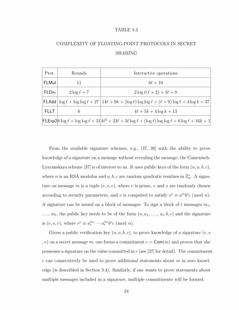
TABLE 3.3

COMPLEXITY OF FLOATING-POINT PROTOCOLS IN SECRET

SHARING

Prot. Rounds Interactive operations

FLMul 11 8`+ 10

FLDiv 2 log `+ 7 2 log `(`+ 2) + 3`+ 8

FLAdd log `+ log log `+ 27 14`+ 9k + (log `) log log `+ (`+ 9) log `+ 4 log k + 37

FLLT 6 4`+ 5k + 4 log k + 13

FLExp26 log `+ log log `+ 314`2 + 23`+ 3` log `+ (log `) log log `+ 6 log `+ 16k + 1

From the available signature schemes, e.g., [37, 38] with the ability to prove

knowledge of a signature on a message without revealing the message, the Camenisch-

Lysyanskaya scheme [37] is of interest to us. It uses public keys of the form (n, a, b, c),

where n is an RSA modulus and a, b, c are random quadratic residues in Z⇤n

. A signa-

ture on message m is a tuple (e, s, v), where e is prime, e and s are randomly chosen

according to security parameters, and v is computed to satisfy ve ⌘ ambsc (mod n).

A signature can be issued on a block of messages. To sign a block of t messages m1

,

. . . , mt

, the public key needs to be of the form (n, a1

, . . . , at

, b, c) and the signature

is (e, s, v), where ve ⌘ am11

· · · amt

t

bsc (mod n).

Given a public verification key (n, a, b, c), to prove knowledge of a signature (e, s

, v) on a secret message m, one forms a commitment c = Com(m) and proves that she

possesses a signature on the value committed in c (see [37] for detail). The commitment

c can consecutively be used to prove additional statements about m in zero knowl-

edge (is describled in Section 3.4). Similarly, if one wants to prove statements about

multiple messages included in a signature, multiple commitments will be formed.

24

TABLE 3.4

COMPLEXITY OF FLOATING-POINT PROTOCOLS IN

HOMOMORPHIC ENCRYPTION

Prot. Rounds Communication sizeComputation complexity

Client Server

FLMul 13 39C + 10D 17 25

FLDiv 2 log `+ 8 4 log `(3C +D) + 18C + 4D 6 log `+ 12 12 log `+ 16

FLAdd

(` log `+ 14 log `+ log log `⇥ 18`+ k + 2`⇥ 21`+ k + 3`⇥

log `+ 45 log `+ 6 log k + 54)D + (15` log `+ 32 log ` log `+ 40 log `

+ log log ` +3` log `+ 19 log `+ 13 log k +14 log k + 2 log `+17 log k + 3 log `

+3 log ` log log `+ 155)C ⇥ log log `+ 125 ⇥ log log `+ 144

FLLT 10(6 log `+ 20)D

k + 14 log k + 41 k + 17 log k + 57+(13 log `+ 63)C

FLExp2

(10`+ ` log `+ 12 log ` 40`+ 2` log `+ 53`+ 3` log `+

15 log ` + log ` log log `+ 35)D + (34` 28 log `+ 3 log ` log log `+

+38 +3` log `+ 26 log `+ 2 log ` log log ` 34 log `

3 log ` log log `+ 107)C +44 +59

The commitment scheme used in [37] is that of Damgard and Fujisaki [51]. The

setup consists of a public key (n, g, h), where n is an RSA modulus, h is a random

quadratic residue in Z⇤n

, and g is an element in the group generated by h. The

modulus n can be the same as or di↵erent from the modulus used in the signature

scheme. For simplicity, we assume that the same modulus is used. To produce

a commitment to x using the key (n, g, h), one randomly chooses r 2 Zn

and sets

25

Com(x, r) = gxhr mod n. When the value of r is not essential, we may omit it and use

Com(x) instead. This commitment scheme is statistically hiding and computationally

binding. The values x, r are called the opening of Com(x, r).

3.4 Zero-Knowledge Proofs of Knowledge

Zero-knowledge proofs of knowledge (ZKPKs) allow one to prove a particular

statement about private values without revealing additional information besides the

statement itself. Following [40], we use notation PK{(vars) : statement} to denote

a ZKPK of the given statement, where the values appearing in the parentheses are

private to the prover and the remaining values used in the statement are known to

both the prover and verifier. If the proof is successful, the verifier is convinced of the

statement of the proof. For example, PK{(↵) : y = g↵1

_ y = g↵2

} denotes that the

prover knows the discrete logarithm of y to either the base g1

or g2

.

In Chapter 4, we utilize four particular ZKPKs: a proof that a ciphertext en-

crypts a value in an specific range, a proof that a ciphertext encrypts one of the two

given values, a proof of plaintext knowledge, and a proof of plaintext multiplication.

Below we specify these ZKPKs more formally using the popular notation of [41],

ZKPK{(S, P ): R}, which states that the prover possesses set S as her secret values,

the values in set P are known to both parties, and the prover proves statement R.

• RangeProof((x, ⇢), (e, L,H)) = ZKPK{(x, ⇢), (e, L,H) : (e = Enc(x, ⇢)) ^ (L x H)}. The prover wishes to prove to the verifier that a ciphertext e en-crypts a value x where x 2 [L,H]. In Chapter 4, we use RangeProof(x, L,H, e)instead of RangeProof((x, ⇢), (e, L,H)) because we do not use parameter ⇢ inthe solutions.

• PK12((a, ⇢), (a0, p1

, p2

)) = ZKPK{(a, ⇢), (a0, p1

, p2

) : (a0 = Enc(a, ⇢)) ^ ((a =p1

) _ (a = p2

))}. Here, the prover wishes to prove to the verifier that a0 =Enc(a, ⇢) is an encryption of one of the two known plaintexts p

1

and p2

.

• PKP((a, ⇢), (a0)) = ZKPK{(a, ⇢), (a0) : (a0 = Enc(a, ⇢))}. The prover wishes toprove to the verifier that he knows the value a that the ciphertext a0 encrypts(and thus that a0 is a valid ciphertext).

26

• PKPM((b, ⇢b

), (a0, b0, c0)) = ZKPK{(b, ⇢b

), (a0, b0, c0) : (b0 = Enc(b, ⇢b

)) ^ (a0 =Enc(a)) ^ (c0 = Enc(c)) ^ (c = ab)}. The prover wishes to prove to the verifierthat c0 encrypts the product of the corresponding plaintexts of a0 and b0, wherethe prover knows the plaintext of b0 (i.e., this is multiplication of an encryptedvalue by a known plaintext value).

For additional information (such as the appropriate choice of parameters), we refer

the reader to [50, 52]. Also, complexity of the above ZKPKs based on homomorphic

encryption can be found in Table 3.5.

TABLE 3.5

COMPLEXITY OF ZKPKS IN HOMOMORPHIC ENCRYPTION

Protocol Rounds Communication sizeComputation complexity

Client Server

RangeProof 1 6 log(H � L)C 5 log(H � L) 6 log(H � L)

PK12 1 4C 3 2

PKPK 1 2.5C 2 2

PKPM 1 4.5C 4 4

Also, in Chapter 5 we use abbreviation Sig(x) and Com(x) to indicate the knowl-

edge of a signature and commitment, respectively. For example, PK{(↵) : Sig(↵) ^

y = Com(↵) ^ (↵ = 0 _ ↵ = 1)} denotes a proof of knowledge of a signature on a

bit committed to in y. Because proving the knowledge of a signature on x in [37]

requires a commitment to x (which is either computed as part of the proof or may

already be available from prior computation), we explicitly include the commitment

27

into all proofs of a signature.

3.5 Security Model

Security of any multi-party protocol (with two or more participants) can be for-

mally shown according to one of the two standard security definitions (see, e.g., [65])

based on hybrid model. The first, weaker security model assumes that the partici-

pants are semi-honest (also known as honest-but-curious or passive), defined as they

follow the computation as prescribed, but might attempt to learn additional infor-

mation about the data from the intermediate results. The second, stronger security

model allows dishonest participants to arbitrarily deviate from the prescribed compu-

tation. The definition of security in the semi-honest model is given in the following.

Definition 1 Let parties P1

, . . ., Pnp

engage in a protocol ⇧ that computes a (possi-

bly probabilistic) np-ary function f : ({0, 1}⇤)np ! ({0, 1}⇤)np, where Pi

contributes

input ini

and receives output outi

. Let VIEW⇧

(Pi

) denote the view of participant

Pi

during the execution of protocol ⇧. More precisely, Pi

’s view is formed by its

input and internal random coin tosses ri

, as well as messages m1

, . . .,mk

passed be-

tween the parties during protocol execution: VIEW⇧

(Pi

) = (ini

, ri

,m1

, . . .,mk

). Let

I = {Pi1 , Pi2 , . . ., Pi

t

} denote a subset of the participants for t < np and VIEW⇧

(I)

denote the combined view of participants in I during the execution of protocol ⇧

(i.e., VIEW⇧

= (VIEW⇧

(Pi1 , . . .,VIEW⇧

(Pi

t

))) and fI

(in1

, . . ., innp

) denote the pro-

jection of f(in1

, . . ., innp

) on the coordinates in I (i.e., fI

(in1

, . . ., innp

) consists of the

i1

th, . . . , it

th elements that f(in1

, . . ., innp

) outputs). We say that protocol ⇧ is t-

private in the presence of semi-honest adversaries if for each coalition I of size at

most t and all ini

2 {0, 1}⇤ there exists a probabilistic polynomial time simulator SI

such that {SI

(inI

, fI

(in1

, . . ., innp

)), f(in1

, . . ., innp

)} ⌘ {VIEW⇧

(I), (out1

, . . ., outnp

)},

where inI

= (in1

, . . ., int

) and “⌘” denotes computational or statistical indistinguisha-

bility.

28

In the two-party setting, we have that np = 2, t = 1. The participants’ inputs

in1

, in2

and outputs out1

, out2

are set as described above. In the multi-party setting,

np > 2, t < np/2, and the computational parties are assumed to contribute no

input and receive no output (to ensure that they can be disjoint from the input

and output parties). Then the input parties secret-share their inputs among the

computational parties prior the protocol execution takes place and the output parties

receive shares of the output and reconstruct the result after the protocol termination.

This setting then implies that, in order to comply with the above security definition,

the computation used in protocol ⇧ must be data-oblivious, which is defined as

requiring the sequence of operations and memory accesses used in ⇧ to be independent

of the input.

Security of a protocol in the malicious model is shown according to the ideal/real

simulation paradigm. In the ideal execution of the protocol, there is a trusted third

party (TTP) that evaluates the function on participants’ inputs. The goal is to build

a simulator S who can interact with the TTP and the malicious party and construct

a protocol’s view for the malicious party. A protocol is secure in the malicious

model if the view of the malicious participants in the ideal world is computationally

indistinguishable from their view in the real world where there is no TTP. Also the

honest parties in both worlds receive the desired output. This gives us the following

definition of security in the malicious model.

Definition 2 Let ⇧ be a protocol that computes function f : ({0, 1}⇤)np ! ({0, 1}⇤)np,

with party Pi

contributing input ini

. Let A be an arbitrary algorithm with auxiliary in-

put x and S be an adversary/simulator in the ideal model. Let REAL⇧,A(x),I

(in1

, . . ., innp

)

denote the view of adversary A controlling parties in I together with the honest par-

ties’ outputs after real protocol ⇧ execution. Similarly, let IDEALf,S(x),I

(in1

, . . ., innp

)

denote the view of S and outputs of honest parties after ideal execution of function

f . We say that ⇧ t-securely computes f if for each coalition I of size at most t,

29

every probabilistic A in the real model, all ini

2 {0, 1}⇤ and x 2 {0, 1}⇤, there is

probabilistic S in the ideal model that runs in time polynomial in A’s runtime and

{IDEALf,S(x),I

(in1

, . . ., innp

)} ⌘ {REAL⇧,A(x),I

(in1

, . . ., innp

)}.

30

CHAPTER 4

VOICE RECOGNITIONS

Hidden Markov Model is a popular statistical tool with a large number of applica-

tions in pattern recognition. In some of these applications, such as speaker recogni-

tion, the computation involves personal data that can identify individuals and must

be protected. We thus treat the problem of designing privacy-preserving techniques

for HMM and companion Gaussian mixture model (GMM) computation suitable for

use in speaker recognition and other applications. We provide secure solutions for

both two-party and multi-party computation models and both semi-honest and ma-

licious settings. In the two-party setting, the server does not have access in the clear

to either the user-based HMM or user input (i.e., current observations) and thus the

computation is based on threshold homomorphic encryption, while the multi-party

setting uses threshold linear secret sharing as the underlying data protection mecha-

nism. All solutions use floating-point arithmetic, which allows us to achieve high ac-

curacy and provable security guarantees, while maintaining reasonable performance.

The rest of this chapter is organized as follows: We first talk about the motivation

of this work and our main contributions in Sections 4.1 and 7.1. Then, we provide

background information regarding HMMs and GMMs in Section 4.3. In Section 4.4,

we describe the security model. We then describe our overall solution in the semi-

honest model in Section 4.5. Section 4.5 reports on the results of our implementation,

and in Section 4.6 we present new techniques to enable secure execution of our solution

in the malicious setting.

31

4.1 Motivation

Hidden Markov Models (HMMs) have been an invaluable and widely used tool in

the area of pattern recognition. They have applications in bioinformatics, credit card

fraud detection, intrusion detection, communication networks, machine translation,

cryptanalysis, robotics, and many other areas. An HMM is a powerful statistical tool

for modeling sequences that can be characterized by an underlying Markov process

with unobserved (or hidden) states, but visible outcomes. One important application

of HMMs is voice recognition, which includes both speech and speaker recognition.

For both, HMMs are the most common and accurate approach, and we use this

application as a running example that guides the computation and security model

for this work.

When an HMM is used for the purpose of speaker recognition, usually one party

supplies a voice sample and the other party holds a description of an HMM that

represents how a particular individual speaks and processes the voice sample using its

model and the corresponding HMM algorithms. Security issues arise in this context

because one’s voice sample and HMMs are valuable personal information that must

be protected. In particular, a server that stores hidden Markov models for users is

in possession of sensitive biometric data, which, once leaked to insiders or outsiders,

can be used to impersonate the users. For that reason, it is desirable to minimize

exposure of voice samples and HMMs corresponding to individuals when such data are

being used for authentication or other purposes. To this end, we design solutions for

securely performing computation on HMMs in such a way that no information about

private data is revealed as a result of execution other than the agreed upon output.

This immediately implies privacy-preserving techniques for speaker recognition as

well as other applications of HMMs.

In more detail, in the speaker recognition application the overall process consists

of two phases: (i) feature extraction in the form of creating an HMM and (ii) speaker

32

authentication in the form of evaluating an HMM. The same two phases would need

to be executed in other applications as well. Feature extraction constitutes a one-time

enrollment process, during which information about how user U speaks is extracted

and privately stored at a server or servers that will later authenticate the user (i.e.,

the HMM is not available to the servers in the clear and prevents leakage of user

information and consequently user impersonation by unauthorized parties). At the

time of user authentication, an individual U 0 wanting to gain access to the system as

user U engages in privacy-preserving user authentication by evaluating a voice sample

that U 0 supplies on U ’s HMM that the server stores. This takes the form of a secure

protocol run between the client U 0 and the server. Note that user authentication can

never be performed locally by the client because U 0 can always return the desired

value as the final outcome to the server.

4.2 Contributions

There are three di↵erent types of problems and corresponding algorithms for

HMM computation: the Forward algorithm, the Viterbi algorithm, and the Expecta-

tion Maximization (EM) algorithm. Because the Viterbi algorithm is most commonly

used in voice recognition, we provide a privacy-preserving solution for that algorithm,

but the techniques can be used to securely execute other HMM algorithms as well.

Furthermore, to ensure that Gaussian mixture models (GMMs), which are commonly

used in HMM computation, can be a part of secure computation as well, we integrate

GMM computation in our privacy-preserving solutions.

One significant di↵erence between our and prior work on secure HMM computa-

tion is that we develop techniques for computation on floating-point numbers, which

provide adequate precision and are most appropriate for HMM computation. We

also do not compromise on security, and all of the techniques we develop are prov-

ably secure under standard and rigorous security models, while at the same time

33

providing reasonable performance (we implement the techniques and experimentally

show performance in the semi-honest setting).

To cover as wide of a range of application scenarios as possible, we consider

multiple settings: (i) the two-party setting in which a client interacts with a server

and (ii) the multi-party setting in which the computation is carried out by np > 2

parties, which is suitable for collaborative computation by several participants as

well as secure outsourcing of HMM computation to multiple servers by one or more

computationally limited clients. In the two-party setting, the server should have

no access in the clear to either the user-based (private) HMM or user input (i.e.,

current observations) and thus the server stores the encrypted HMM and computation

proceeds on encrypted data (see Section 4.4.1 for justification of this setup). In the

multi-party setting, on the other hand, threshold linear secret sharing is employed as

the underlying mechanism for privacy-preserving computation.

We provide techniques for both semi-honest and malicious security models using

secure floating-point operations from [11]. Because [11] treats only the semi-honest

setting, equivalent solution secure in the stronger malicious model are not available

for the two-party case based on homomorphic encryption. We thus develop neces-

sary protocols to support general secure floating-point operations in the two-party

computation setting based on homomorphic encryption.

To summarize, our contributions consist of developing provably secure HMM and

GMM computation techniques based on Viterbi algorithm using floating-point arith-

metic. Our techniques are suitable for homomorphic encryption and secret sharing

computations in a variety of settings and are designed with their e�ciency in mind,

which we evaluate through experimental results of an implementation.

34

4.3 Hidden Markov Models and Gaussian Mixture Models

A Hidden Markov Model (HMM) is a statistical model that follows the Markov

property with hidden states, but visible outcomes. The inputs are a sequence of

observations, and for each sequence of observations (or outcomes), the computation

consists of determining a path of state transitions which is the likeliest among all

paths that could produce the given observations. An HMM consists of: 1) N states,

2) M possible outcomes, 3) a vector ⇡ = h⇡1

, . . ., ⇡N

i that contains the initial state

probability distribution, 4) a matrix A of size N ⇥ N that contains state transition

probabilities, 5) a matrix B of size N⇥M that contains output probabilities. In most

cases, matrix B is computed based on observations (X1

, . . ., XT

). Therefore, we refer

to the elements of B chosen based on, or computed from, the current observations as

N ⇥ T matrix �. More information can be found in [9].

GMMs are mixtures of Gaussian distributions that represent the overall distribu-

tion of observations. In the case of HMMs, we use a GMM to compute the output

probability of state number j (Sj

) producing an observation at time k as follows:

�jk

=↵X

i=1

wi

e�12 (Xk

�µ

i

)

T

⌃

�1i

(X

k

�µ

i

) (4.1)

where Xk

is a vector of size f that represents the random variable corresponding

to the observation at time k. The parameter ↵ is the total number of mixture

components. µi

is a mean vector of ith component with size f ; also, ith component

has a covariance matrix ⌃i

of size f ⇥ f . The components are added together, each

weighted by a mixture weight wi

, to produce the probability distribution of state Sj

when the observed random variable is Xk

. We use notation µ, ⌃, and w to refer to

the sequence of µi

, ⌃i

, and wi

, respectively, for i = 1, . . .,↵.

In this work, we focus on the Viterbi algorithm (with complexity of O(TN2))

used in speaker recognition. In Algorithm 1, we provide a brief description of HMM

35

Algorithm 1: HMM algorithmInput: N, T, ⇡, A,↵, w, µ,⌃, and XOutput: P ⇤ that is the probability of the most likely path for a given sequenceof observations and q⇤ = hq⇤

1

, . . ., q⇤T

i that denotes the most likely path itself.

1. For j = 1 to N and k = 1 to T , compute �jk

as in Equation 4.1 using ↵, wi

’s,µi

’s, ⌃i

’s, and Xk

.

2. Set � = hN, T, ⇡, A, �i.

(a) Initialization Step: for i = 1 to N do

i. �1

(i) = ⇡i

�i1

ii. 1

(i) = 0

(b) Recursion Step: for k = 2 to T and j = 1 to N do

i. �k

(j) =

✓max1iN

[�k�1

(i)aij

]

◆�jk

ii. k

(j) = argmax1iN

[�k�1

(i)aij

]

(c) Termination Step:

i. P ⇤ = max1iN

[�T

(i)]

ii. q⇤T

= argmax1iN

�T

(i)

iii. for k = T � 1 to 1 do q⇤k

= k+1

(q⇤k+1

)

3. Return hP ⇤, q⇤i

computation by computing the Viterbi algorithm (step 2). The computation uses

dynamic programming to store intermediate probabilities in �, after which the path

of the maximum likelihood is computed and placed in q⇤. For additional information,

we refer the reader to [9].

4.4 Framework

In this section, we introduce two categories of secure computation that we consider

in this work (two-party and multi-party), and precisely define the computation to be

carried out.

36

4.4.1 Two-Party Computation

The first category of secure computation that we consider is secure two-party

computation. Without loss of generality, we will refer to the participants as the client

and the server. Using speaker recognition as the example application, the setting can

be described as follows: the client possesses a voice sample, the server stores a model

that represents how a registered user speaks, and user authentication is performed

by conducting HMM computation on the client’s and server’s inputs. Therefore,

for the purposes of this work, we assume that the client owns the observations to

an HMM, i.e., X1

, . . ., XT

, and the server holds the parameters of the HMM and

GMM, i.e., N , vector ⇡, matrix A, ↵, mixture weights w, vectors µ, and matrices ⌃.

Because even the parameters of HMM might reveal information about the possible

input observations, to build a fully privacy-preserving solution in which the server

does not learn information about user biometrics, the server should not have access

to the HMM parameters in the clear. For that reason, we assume that the server

holds the parameters ⇡, A, B, w, µ, and ⌃ in an encrypted form and computation

proceeds on encrypted data. While there are other underlying techniques for secure

two-party computation (such as garbled circuit evaluation), we view storing HMM

data encrypted at the server and evaluating the function on encrypted data as the

best option, despite high computational overhead associated with this approach. If

encryption is not used, the HMM values will need to be split into random shares,

with one share of each value stored by the client and the other share stored by the

server. This creates multiple issues, one of which is that the client’s state is large and

the shares of the HMM must be present on each device from which the client wants

to authenticate. The second issue is that a malicious user will need to be forced to

enter the original HMM data into each authentication session to avoid tampering

with the authentication process, which is generally not known how to do.

To permit the computation to take place on encrypted data, we resort to an

37

encryption scheme with special properties, namely, semantically secure additively

homomorphic public-key encryption scheme. Furthermore, to ensure that neither the

server can decrypt the data it stores, nor the (untrusted) client can decrypt the data

(or a function thereof) without the server’s consent, we utilize a (2, 2)-threshold en-

cryption scheme. Informally, it means that the decryption key is partitioned between

the client and the server, and each decryption requires that both of them participate.

This means that the client and the server can jointly carry out the HMM compu-

tation and make the result available to either or both of them. For concreteness of

exposition, we will assume that the server learns the outcome.

We obtain that in the two-party setting, the client and the server share the decryp-

tion key to a semantically secure additively homomorphic (2, 2)-threshold public-key

encryption scheme. The client has private input X1

, . . ., XT

and its share of the de-

cryption key sk; the server has input Encpk

(⇡i

) for i 2 [1, N ], Encpk

(aij

) for i 2 [1, N ]

and j 2 [1, N ], Encpk

(wi

) for i 2 [1,↵], encryption of each element of µi

and ⌃i

for

i 2 [1,↵], and its share of sk. The computation consists of executing the Viterbi algo-

rithm on their inputs, at the end of which the server learns P ⇤ and q⇤i

for i = 1, . . ., T .

The size of the problem, i.e., parameters N , T , ↵, and f , are assumed to be known

to both parties.

4.4.2 Multi-Party Computation

The second category of secure computation that we consider is secure multi-party

computation on HMMs. In this setting, either a number of parties hold inputs to a

multi-observer HMM or one or more clients wish to outsource HMM computations to

a collection of servers. More generally, we divide all participants into three groups: (i)

the input parties who collectively possess the private inputs, (ii) the computational

parties who carry out the computation, and (iii) the output parties who receive the

result(s) of the computation. These groups can be arbitrarily overlapping, which

38

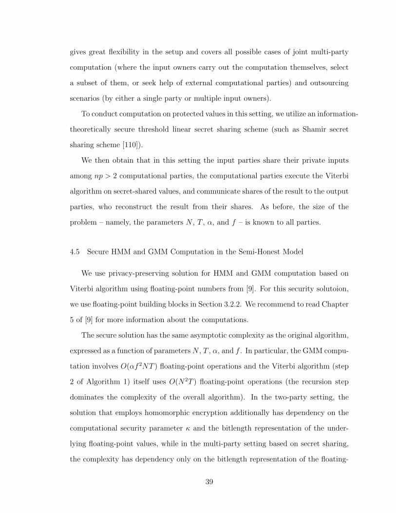
gives great flexibility in the setup and covers all possible cases of joint multi-party

computation (where the input owners carry out the computation themselves, select

a subset of them, or seek help of external computational parties) and outsourcing

scenarios (by either a single party or multiple input owners).

To conduct computation on protected values in this setting, we utilize an information-

theoretically secure threshold linear secret sharing scheme (such as Shamir secret

sharing scheme [110]).

We then obtain that in this setting the input parties share their private inputs

among np > 2 computational parties, the computational parties execute the Viterbi

algorithm on secret-shared values, and communicate shares of the result to the output

parties, who reconstruct the result from their shares. As before, the size of the

problem – namely, the parameters N , T , ↵, and f – is known to all parties.

4.5 Secure HMM and GMM Computation in the Semi-Honest Model

We use privacy-preserving solution for HMM and GMM computation based on

Viterbi algorithm using floating-point numbers from [9]. For this security solutoion,

we use floating-point building blocks in Section 3.2.2. We recommend to read Chapter

5 of [9] for more information about the computations.

The secure solution has the same asymptotic complexity as the original algorithm,

expressed as a function of parametersN , T , ↵, and f . In particular, the GMM compu-

tation involves O(↵f 2NT ) floating-point operations and the Viterbi algorithm (step

2 of Algorithm 1) itself uses O(N2T ) floating-point operations (the recursion step

dominates the complexity of the overall algorithm). In the two-party setting, the

solution that employs homomorphic encryption additionally has dependency on the

computational security parameter and the bitlength representation of the under-

lying floating-point values, while in the multi-party setting based on secret sharing,

the complexity has dependency only on the bitlength representation of the floating-

39

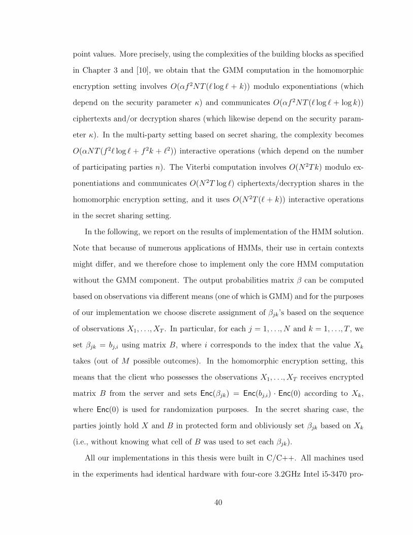
point values. More precisely, using the complexities of the building blocks as specified

in Chapter 3 and [10], we obtain that the GMM computation in the homomorphic

encryption setting involves O(↵f 2NT (` log ` + k)) modulo exponentiations (which

depend on the security parameter ) and communicates O(↵f 2NT (` log ` + log k))

ciphertexts and/or decryption shares (which likewise depend on the security param-

eter ). In the multi-party setting based on secret sharing, the complexity becomes

O(↵NT (f 2` log ` + f 2k + `2)) interactive operations (which depend on the number

of participating parties n). The Viterbi computation involves O(N2Tk) modulo ex-

ponentiations and communicates O(N2T log `) ciphertexts/decryption shares in the

homomorphic encryption setting, and it uses O(N2T (` + k)) interactive operations

in the secret sharing setting.

In the following, we report on the results of implementation of the HMM solution.

Note that because of numerous applications of HMMs, their use in certain contexts

might di↵er, and we therefore chose to implement only the core HMM computation

without the GMM component. The output probabilities matrix � can be computed

based on observations via di↵erent means (one of which is GMM) and for the purposes

of our implementation we choose discrete assignment of �jk

’s based on the sequence

of observations X1

, . . ., XT

. In particular, for each j = 1, . . ., N and k = 1, . . ., T , we

set �jk

= bj,i

using matrix B, where i corresponds to the index that the value Xk

takes (out of M possible outcomes). In the homomorphic encryption setting, this

means that the client who possesses the observations X1

, . . ., XT

receives encrypted

matrix B from the server and sets Enc(�jk

) = Enc(bj,i

) · Enc(0) according to Xk

,

where Enc(0) is used for randomization purposes. In the secret sharing case, the

parties jointly hold X and B in protected form and obliviously set �jk

based on Xk

(i.e., without knowing what cell of B was used to set each �jk

).

All our implementations in this thesis were built in C/C++. All machines used

in the experiments had identical hardware with four-core 3.2GHz Intel i5-3470 pro-

40

Figure 4.1. Performance of integer HMM’s building blocks in thehomomorphic encryption setting.

cessors with Red Hat Linux 2.6.32 and were connected via a 1Gb LAN. Only one

core was used during the experiments (i.e., multi-threading was not used).

In what follows, we first describe our homomorphic encryption experiments fol-

lowed by the experiments in the secret sharing setting. In our implementations we

represent floating-point numbers using 32-bit significands and (signed) 9-bit expo-

nents (plus sign and zero bits as described earlier in this work).

In the homomorphic encryption setting, we utilized (2, 2)-threshold Paillier en-

cryption, which was implemented using Miracl library [47] for large number arith-

metic. The experiments we report were conducted using a 1536-bit modulus for

Paillier encryption. Because performance of our building blocks is not available in

prior literature, we provide runtimes of integer and floating-point operations used in

our implementation in Figures 4.1 and 4.2 and overall HMM computation in Fig-

41

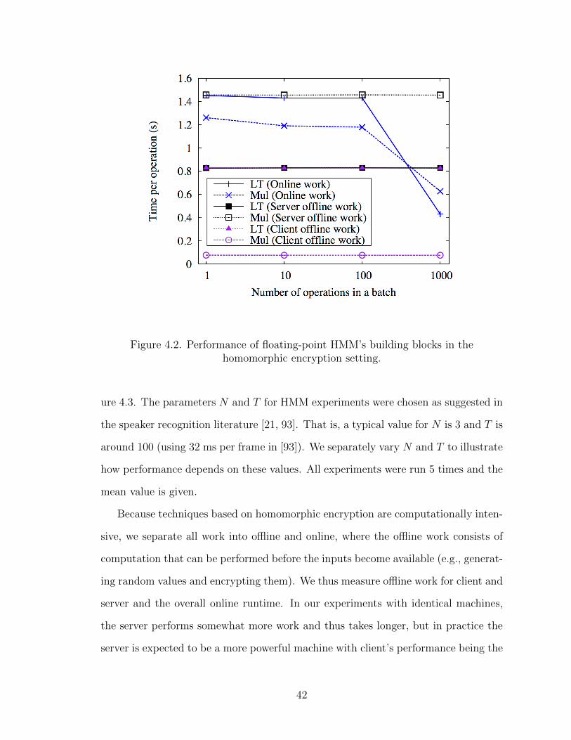
Figure 4.2. Performance of floating-point HMM’s building blocks in thehomomorphic encryption setting.

ure 4.3. The parameters N and T for HMM experiments were chosen as suggested in

the speaker recognition literature [21, 93]. That is, a typical value for N is 3 and T is

around 100 (using 32 ms per frame in [93]). We separately vary N and T to illustrate

how performance depends on these values. All experiments were run 5 times and the

mean value is given.

Because techniques based on homomorphic encryption are computationally inten-

sive, we separate all work into o✏ine and online, where the o✏ine work consists of

computation that can be performed before the inputs become available (e.g., generat-

ing random values and encrypting them). We thus measure o✏ine work for client and

server and the overall online runtime. In our experiments with identical machines,

the server performs somewhat more work and thus takes longer, but in practice the

server is expected to be a more powerful machine with client’s performance being the

42

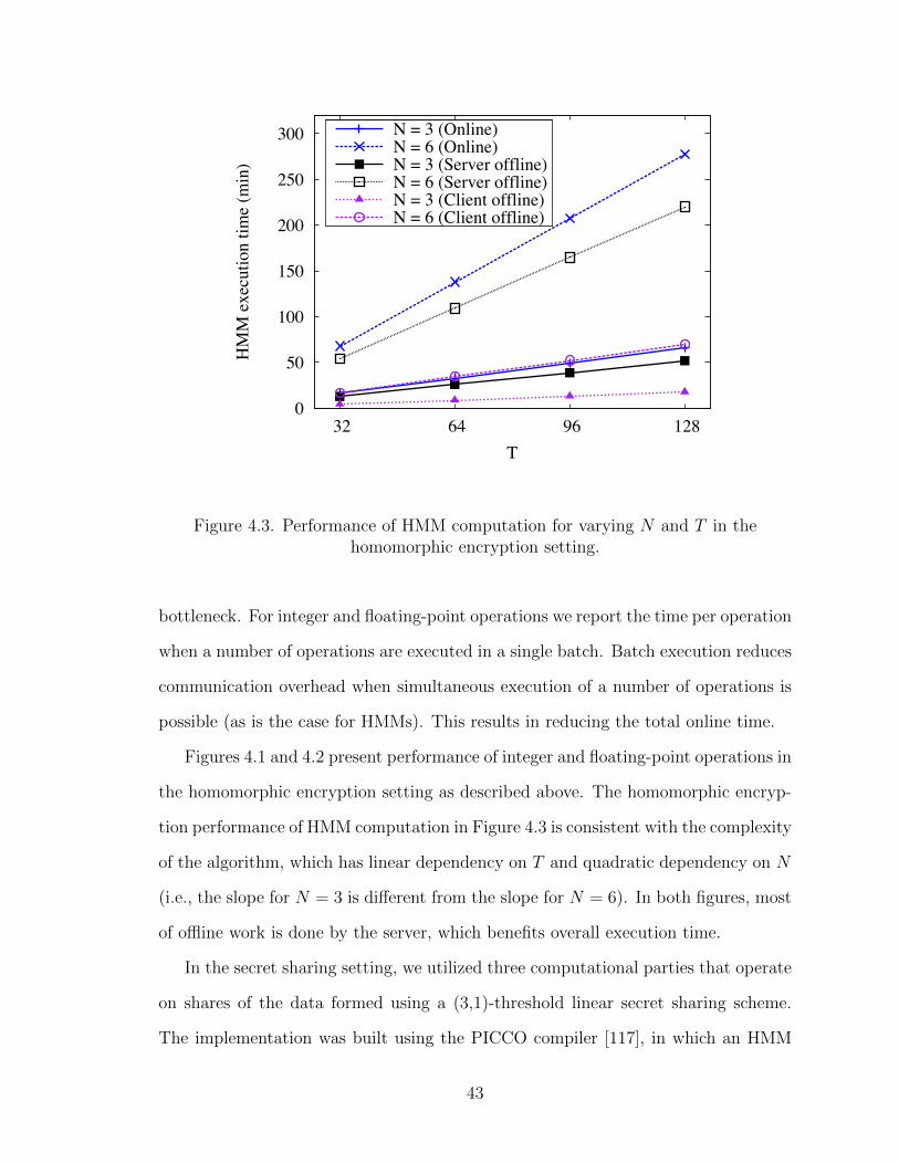
0

50

100

150

200

250

300

32 64 96 128

HM

M e

xecu

tion

time

(min

)

T

N = 3 (Online)N = 6 (Online)N = 3 (Server offline)N = 6 (Server offline)N = 3 (Client offline)N = 6 (Client offline)

Figure 4.3. Performance of HMM computation for varying N and T in thehomomorphic encryption setting.

bottleneck. For integer and floating-point operations we report the time per operation

when a number of operations are executed in a single batch. Batch execution reduces

communication overhead when simultaneous execution of a number of operations is

possible (as is the case for HMMs). This results in reducing the total online time.

Figures 4.1 and 4.2 present performance of integer and floating-point operations in

the homomorphic encryption setting as described above. The homomorphic encryp-

tion performance of HMM computation in Figure 4.3 is consistent with the complexity

of the algorithm, which has linear dependency on T and quadratic dependency on N

(i.e., the slope for N = 3 is di↵erent from the slope for N = 6). In both figures, most

of o✏ine work is done by the server, which benefits overall execution time.

In the secret sharing setting, we utilized three computational parties that operate

on shares of the data formed using a (3,1)-threshold linear secret sharing scheme.

The implementation was built using the PICCO compiler [117], in which an HMM

43

0

10

20

30

40

32 64 96 128

HM

M e

xecu

tion

time

(s)

T

N = 3N = 6

Figure 4.4. Performance of HMM computation for varying N and T in thesecret sharing setting.

program written in an extension of C was compiled into its secure distributed imple-

mentation. PICCO is a source-to-source compiler that produces a C program and

utilizes the GMP [4] library for the underlying arithmetic and OpenSSL [6] imple-

mentation of AES for protecting communication. All arithmetic was performed in

field Fp

for a 114-bit prime p (the modulus size was determined as described in [117]).

The results of HMM experiments are given in Figure 4.4. While separation between

online and o✏ine work is also possible in this setting (e.g., the parties generate a

large number of random values throughout the protocol execution), we do not dis-

tinguish between these types of work and list the overall performance in the online

category. This is in part because we use an existing tool for our experiments and

in part because the secret sharing performance is orders of magnitude faster than

encryption-based two-party computation and is already practical.

In conclusion, we note that our two-party setting was constrained in terms of the

44

tools that could be employed for secure computation. That is, in order to provably

protect HMMs from the server, we have to resort to strong protection mechanisms

such as homomorphic encryption, the threshold version of which was required to

ensure that no individual party could independently decrypt ciphertexts and learn

unauthorized information. In general, alternative techniques of better performance

(such as garbled circuit) are possible and even additively homomorphic encryption can

be substantially faster (see, e.g., [33]) when threshold decryption is not required. One

suggestion for improving performance of the two-party setting for this application is to

involve neutral third parties, which would allow for the use of multi-party techniques.

4.6 Secure HMM and GMM Computation in the Malicious Model

We next show how strengthen the solution to maintain security in the presence of

malicious participants who can arbitrarily deviate from the prescribed behavior. The

solution for the multi-party setting based on secret sharing, covered in Section 4.6.1.

Most of the section is dedicated to the two-party setting based on homomorphic en-

cryption, where in Section 4.6.2 we describe the necessary components for building a

solution secure against malicious adversaries and in Sections 4.6.2.1–4.6.2.6 present

protocols for two-party multiplication, comparison, truncation, inversion, prefix mul-

tiplication, and bit decomposition, respectively, together with their malicious-model

security analysis.

4.6.1 Multi-Party Setting

The security of the solution in the secret sharing setting can be extended to the

malicious security model. In that case, to show security in the presence of malicious

adversaries, we need to ensure that (i) all participants prove that each step of their

computation was performed correctly and that (ii) if some dishonest participants

quit, others will be able to reconstruct their shares and proceed with the rest of

45

the computation. The above is normally achieved using a verifiable secret sharing

scheme (VSS), and a large number of results have been developed over the years.

More information can be found in [9].

4.6.2 Two-Party Setting

To show security of our solution in the presence of malicious adversaries in the

homomorphic encryption setting, we likewise need to enforce correct execution of all

operations. However, unlike the secret sharing setting, this time security no longer

follows from prior work and requires new tools.

To ensure that both participants follow all steps of the computation, we employ

zero-knowledge proofs of knowledge from Section 3.4. Because such proofs are usually

tied to the internal workings of the underlying homomorphic encryption scheme, we

develop our solution based on the Paillier encryption scheme.

Our approach consists of using designed protocols secure in the presence of ma-

licious adversaries for a number of building blocks used to build floating-point oper-

ations. Then after applying Canetti’s composition theorem [44], we can guarantee

security of larger building blocks and the overall solution. To determine which build-

ing blocks need to be implemented in the stronger security model with fully malicious

participants, we analyze each floating-point operation used in this work.

• FLMul is implemented using protocols Trunc, LT, OR, XOR, and Mul as thebuilding blocks. Trunc in turn depends on TruncPR and LT protocols1. OR andXOR protocols are built directly from Mul. This means that we need to realizemalicious versions of multiplicationMul, truncation TruncPR, and comparison LT.

• Besides some of the building blocks listed above, FLDiv additionally uses SDiv,which in turn is built using Mul and TruncPR protocols. Thus, no additionalprotocols are needed.

1Throughout this description we don’t describe the functionality of each building block. Such

description will be given only for the building blocks that we need to implement in the malicious

model.

46

• FLAdd calls new building blocks EQ, Pow2, BitDec, PreOR, and Inv. Our imple-mentation of EQ is built on LT and Mul. Pow2 calls BitDec and PreMul. PreOrcalls PreMul and Mod2, which is equivalent to Trunc.

• FLLT does not call any new building blocks.

• Similarly, FLExp calls only integer building blocks discussed above and FLMulthat can be assembled from integer building blocks.

To summarize, we need to provide implementations of six functionalities secure

in the malicious model, which are described next:

• Enc(xy) MalMul(Enc(x),Enc(y)) is a fundamental building block, which per-forms multiplication of its two encrypted input values x and y.

• Enc(b) MalLT(Enc(x),Enc(y), `) performs comparison of two encrypted val-ues x and y of size ` and outputs encrypted bit b, where b = 1 i↵ x < y.

• Enc(y) MalTruncPR(Enc(x), `, k) truncates k bits of encrypted x, which hasbitlength `. The output is probabilistic, where the least significant bit of theresult y may di↵er from that of bx/2kc.2

• Enc(y) MalInv(Enc(x)) produces (encrypted) inversion y = x�1 of encrypted x.

• Enc(y1

), ...,Enc(yk

) MalPreMul(Enc(x1

), ..., Enc(xk

)) performs prefix multi-plication of k non-zero encrypted values x

1

, . . ., xk

, where the result is computedas y

i

=Q

i

j=1

xj

for each i 2 [1, k].

• Enc(xk�1

), ...,Enc(x0

) MalBitDec(Enc(a), `, k) extracts k least significant bitsof (encrypted) x, where ` is the bitlength of x.

In the rest of this section we treat one protocol (two-party setting based on ho-

momorphic encryption) at a time and report performance of each new protocol in

the malicious model in Table 4.1.

4.6.2.1 Secure Multiplication

Now we describe a two-party multiplication protocol secure in the presence of a

malicious participant. In this protocol, both parties hold Enc(x),Enc(y) without any

2We note that such probabilistic version is su�cient in some cases, while in others the function

can be changed to always produce correct truncation with the use of extra comparison.

47

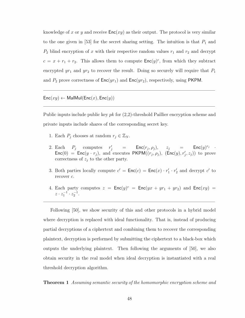
knowledge of x or y and receive Enc(xy) as their output. The protocol is very similar

to the one given in [53] for the secret sharing setting. The intuition is that P1

and

P2

blind encryption of x with their respective random values r1

and r2

and decrypt

c = x + r1

+ r2

. This allows them to compute Enc(y)c, from which they subtract

encrypted yr1

and yr2

to recover the result. Doing so securely will require that P1

and P2

prove correctness of Enc(yr1

) and Enc(yr2

), respectively, using PKPM.

Enc(xy) MalMul(Enc(x),Enc(y))

Public inputs include public key pk for (2,2)-threshold Paillier encryption scheme and

private inputs include shares of the corresponding secret key.

1. Each Pj

chooses at random rj

2 ZN

.

2. Each Pj

computes r0j

= Enc(rj

, ⇢j

), zj

= Enc(y)rj ·Enc(0) = Enc(y · r

j

), and executes PKPM((rj

, ⇢j

), (Enc(y), r0j

, zj

)) to provecorrectness of z

j

to the other party.

3. Both parties locally compute c0 = Enc(c) = Enc(x) · r01

· r02

and decrypt c0 torecover c.

4. Each party computes z = Enc(y)c = Enc(yx + yr1

+ yr2

) and Enc(xy) =z · z�1

1

· z�1

2

.

Following [50], we show security of this and other protocols in a hybrid model

where decryption is replaced with ideal functionality. That is, instead of producing

partial decryptions of a ciphertext and combining them to recover the corresponding

plaintext, decryption is performed by submitting the ciphertext to a black-box which

outputs the underlying plaintext. Then following the arguments of [50], we also

obtain security in the real model when ideal decryption is instantiated with a real

threshold decryption algorithm.

Theorem 1 Assuming semantic security of the homomorphic encryption scheme and

48

security of the building blocks, the above MalMul is secure in the malicious setting in

the hybrid model with ideal decryption.

Proof: We prove security of MalMul based on Definition 2. Because this protocol

is completely symmetric, without loss of generality we assume P1

is malicious. In

that case, in the ideal world a simulator S1

locates between P1

and the TTP and

simulates P1

’s view after receiving Enc(x) and Enc(y), as well as Enc(xy) from the

TTP. During step 2, S1

receives r01

and z1

, and acts as a verifier for PKPM (extracting

r1

). Then, S1

sets r02

= Enc(w � r1

� x) for a randomly chosen w 2 ZN

, computes

z2

= (Enc(xy))�1(Enc(y))w�r1 , and uses the simulator of PKPM to interact with P1

and prove validity of r02

, z2

. During step 3, S1

sends w as the decrypted value c to P1

.

To show that P1

’s output at the end of the simulation corresponds to correct

Enc(xy), recall that the simulator sets r2

= w� r1

� x. Thus, w = x+ r1

+ r2

in step

3 is exactly what the simulator needs to decrypt. Therefore, P1

correctly computes

the output in step 4.

To show that the simulated view is indistinguishable from the view in the hybrid

model (with ideal decryption), we note that the simulator produces encrypted val-

ues in step 2, which are indistinguishable from ciphertexts sent during the protocol

execution because of semantic security of the encryption scheme. Similarly, the simu-

lation of PKPM is indistinguishable from real execution due to its security properties.

Lastly, the value w returned by the simulator in step 3 is distributed identically to

the value c decrypted during protocol execution. We also note that both during the

simulation and real execution the computation aborts only when a malicious party

fails to correctly complete. 2

4.6.2.2 Secure Comparison

Our comparison protocol secure in the malicious model is given next. In what

follows, we use the fact that (�1)b = 1 � 2b and (�1)1�b = 2b � 1 when b is a bit.

49

We also express a01

as Enc(1 + 2b1

b2

� b1

� b2

) and a02

as Enc(b1

+ b2

� 2b1

b2

).

Enc(b) MalLT(Enc(x),Enc(y), `)

Public inputs include public key pk for a (2,2)-threshold Paillier encryption scheme

and private inputs consist of shares of the corresponding secret key.

1. Each Pj

sets e1

= Enc(1, 0), e�1

= Enc(�1, 0) = (e1

)�1, and Enc(c) = Enc(x �y) = Enc(x) · Enc(y)�1.

2. Each Pj

chooses bj

2 {0, 1}, rj

, r0j

2 {0, 1}`+ at random s.t. rj

> r0j

, and sendsto P

3�j

z(j,1)

= Enc(bj

, ⇢j

), z(j,2)

= Enc(rj

, ⇢0j

) and z(j,3)

= Enc(r0j

, ⇢00j

). Pj

exe-cutes PK12((b

j

, ⇢j

), (z(j,1)

, 0, 1)), RangeProof(rj

, 0, H, z(j,2)

), RangeProof(r0j

, 0, H,z(j,3)

), and RangeProof(rj

� r0j

, 1, H, z(j,2)

· z�1

(j,3)

) to prove that z(j,1)

, z(j,2)

, and

z(j,3)

are well-formed, where H = 2`+ � 1.

3. Each party locally computes z(j,4)

= Enc(1 � 2bj

) = e1

· (z(j,1)

)�2 and z(j,5)

=Enc(2b

j

� 1) = (z(j,1)

)2 · e�1

.

4. P1

computes z6

= Enc((1 � 2b1

)c)) = Enc(c)1�2b1 · Enc(0,↵1

), where ↵1

isnewly selected as randomness during encryption, z

7

= Enc(r1

(1� 2b1

)c) = zr16

,

and z8

= Enc((2b1

� 1)r01

) = zr

01

(1,5)

, and sends to P2

z6

, z7

, and z8

. P1

also executes PKPM((1 � 2b1

mod N, ⇢�2

1

), (Enc(c), z(1,4)

, z6

)), PKPM((r1

, ⇢01

+↵1

), (z6

, z(1,2)

, z7

)), and PKPM((r01

, ⇢001

), (z(1,5)

, z(1,3)

, z8

)) to prove that z6

, z7

,and z

8

are well-formed.

5. Each party locally computes a3

= Enc(r1

(1� 2b1

)c) + (2b1

� 1)r01

) = z7

· z8

.

6. P2

computes z06

= Enc(b1

b2

) = zb2(1,1)

· Enc(0,↵2

), z07

= a1�2b23

· Enc(0,↵3

), where↵2

and ↵3

are newly selected as randomness during encryption, z08

= (z07

)r2 ,

and z09

= zr

02

(2,5)

, and sends to P1

z06

, z07

, z08

, and z09

. P2

executes PKPM((b2

, ⇢2

+

↵2

), (z(1,1)

, z(2,1)

, z06

)), PKPM((1� 2b2

mod N, ⇢�2

2

+ ↵3

), (a3

, z(2,4)

, z07

)),PKPM((r

2

, ⇢02

), (z07

, z(2,2)

, z08

)), and PKPM((r02

, ⇢002

), (z(2,5)

, z(2,3)

, z09

)) to prove thatz06

, z07

, z08

, and z09

are well-formed.

7. Each party locally computes a03

= z08

· z09

.

8. The parties decrypt a03

. If the decrypted value is < N2/2, output z(1,1)

· z(2,1)

·(z0

6

)�2; otherwise, output e1

(z06

)2 · (z(1,1)

· z(2,1)

)�1.

50

Our protocol closely follows the logic of the semi-honest solution [9], where we

additionally need to employ zero-knowledge proofs to provide each party with the

ability to verify that the computation was performed correctly by the other party.

We do not explicitly compute both a01

and a02

as in the semi-honest version, but rather

compute and return either a01

or a02

in step 8 after decrypting the content of a03

. We

also explicitly keep track of random values used for creating ciphertexts and use them

as input into ZKPKs. This ensures that the protocol is fully specified.

Our security result can be stated as given next. Recall that we use a hybrid model

with ideal decryption, which we then replace with a real instantiation of threshold

decryption.

Theorem 2 Assuming semantic security of the homomorphic encryption and secu-

rity of the building blocks, MalLT protocol is secure in the presence of a malicious

adversary in the hybrid model with ideal decryption.

Proof: We prove security of MalLT based on Definition 2. We separately consider

the cases when P1

is malicious and when P2

is malicious. In the ideal world, we build

a simulator Sj

that is located between malicious party Pj

and the TTP and simulates

Pj

’s view of the protocol after querying the TTP for Pj

’s output.

First, we treat the case of malicious P1

and build the corresponding simulator S1

.

Upon obtaining the input Enc(x),Enc(y), `, S1

queries the TTP for Enc(b). In step

1, S1

performs the same computation as P2

. In step 2, S1

acts as a verifier for P1

’s

ZKPKs PK12 and RangeProofs and extracts P1

’s input to the proofs. It also chooses a

random bit w and computes Enc(b⇤) = Enc(b)1�w · (e1

(Enc(b))�1)w = Enc(b · (1�w)+

(1�b)·w) = Enc(b�w). In other words, if w = 0 then b⇤ = b and otherwise b⇤ = 1�b.

S1

similarly computes Enc(b2

) = Enc(b⇤ � b1

) and chooses and encrypts two random

values r2

and r02

according to the protocol. S1

now simulates P2

’s proofs PK12 and

RangeProof using Enc(b2

), Enc(r2

), and Enc(r02

). In steps 3–5, S1

acts like P2

, i.e., S1

51

performs the prescribed computation in steps 3 and 5 and acts as a verifier for P1

’s

proofs PKPMs during step 4. During step 6, S1

computes z06

= Enc(b2

)b1 · Enc(0, �1

)

and z07

= a1�2w

0

3

· Enc(0, �2

), where w0 is a newly generated random bit and �1

, �2

correspond to freshly chosen randomness during encryption. S1

also computes the

remaining z08

and z09

according to the protocol. Note that using random w0 in place

of b2

makes the content of ciphertexts z07

and z08

inconsistent with other encrypted

values, but P1

cannot tell this fact due to security of the encryption scheme. S1

then

simulates the PKPM proofs in step 6. Finally, in step 7, S1

sends a positive properly

chosen value c 2 [0, N2/2) to P1

if w = 0, and a negative properly chosen value

c 2 [N2/2, N2) otherwise. To form c, S1

randomly samples the distribution of the

absolute value of x�y (using application-specific knowledge of distributions of x and

y); let the randomly chosen value be denoted by d. S1

then sets c = (r1

·d�r01

)r2

�r02

if w = 0 and c = N2 � (r1

· d � r01

)r2

+ r02

otherwise. Note that ciphertexts z07

and

z08

are not used by the simulator beyond step 6 and thus their contents do not a↵ect

correctness of the output.

To show that the view simulated by S1

results in P1

obtaining correct output, we

note that w = b1

�b2

�b (because b1

= b2

�b�w). Now, if w = 0, b = b1

�b2

= b1

+b2

�

2b1

b2

. Thus, S1

needs to produce a positive value (< N2/2) as the decryption of a03

in

step 8, so that z(1,1)

· z(2,1)

· (z06

)�2 = Enc(b1

+ b2

� 2b1

b2

) = Enc(b) is produced as the

output in step 8. Otherwise, if w = 1, b = 1�b1

�b2

= 1�(b1

�b2

) = 1�b1

�b2

+2b1

b2

.

Thus, S1

needs to produce a negative value (� N2/2) as the decryption of a03

in step

8, so that P1

uses e1

(z06

)2 · (z(1,1)

z(2,1)

)�1 = Enc(1 + 2b1

b2

� b1

� b2

) = Enc(b) as the

output.


is indistinguishable from P1

’s view in

the hybrid model (with ideal decryption), we note that most values the simulator

sends to P1

(e.g., steps 2 and 6) are encrypted and thus are indistinguishable from

ciphertexts sent during the protocol execution because of semantic security of the

52

encryption scheme. Similarly, the simulations of PK12, RangeProofs, and PKPMs are

indistinguishable from real execution due to their security properties. The only value

that S1

provides to P1

in the clear is the decryption of a03

in step 7. This value

was chosen by S1

in the same way as during the protocol after randomly sampling

the absolute value of x � y according to what is known about distributions of x

and y. Thus, P1

is unable to distinguish the value received during the simulation

from the value received during the protocol execution. We also note that during the

simulation S1

aborts the computation in exactly the same circumstances when the

computation is aborted in the real execution (namely, when a ZKPK does not verify)

and thus the simulation cannot be distinguished from real execution on the grounds

of computation termination.

Now let P2

be malicious. We build a simulator S2

that constructs P2

’s view

similar to the way S1

did for P1

. Most of S2

’s computations are the same as S1

’s

computations, and thus we concentrate on the di↵erences. In this case, S2

computes

Enc(b⇤) in step 2 in the same way S1

did (i.e., by choosing a random bit w and using

b⇤ = b � w) and then sets Enc(b1

) = Enc(b⇤ � b2

). In step 4, S2

selects a random

bit w0 and a random number ⇠1

to be used as randomness during encryption and

computes z6

= Enc(c)1�2w

0 · Enc(0, ⇠1

). S2

also computes z7

and z8

according the

protocol and simulates the PKPM proofs (step 4). Note that using w0 instead of b1

(which S2

doesn’t know) in the computation of z6

makes the content of ciphertexts

z7

, a3

, z07

, z08

, and a03

inconsistent with other encrypted values, but P2

is unable to tell

this fact because of security of the encryption scheme. In steps 5 and 6, S2

acts like

P1

. Finally, in step 7, S2

provides a positive properly chosen value c 2 [0, N2/2) to

P2

if w was 0, and otherwise a negative properly chosen value c 2 [N2/2, N2). Note

that none of incorrectly formed ciphertexts (z6

, z7

, a3

, z07

, z08

, and a03

) are used in the

computation of the protocol’s output and correctness of the result is not a↵ected.

Correctness of the output that P2

learns at the end of S2

’s simulation can be

53

shown in a way similar to that of S1

’s simulation. In other words, we now also have

that w = b1

� b2

� b and producing a positive value as the decryption of a03

when

w = 0 and producing a negative value when w = 1 results in P2

computing Enc(b).

What remains to show is that the view simulated by S2

is indistinguishable from

P2

’s view in the hybrid model. Similar to S1

’s case, we have that all values that S2

sends to P2

are either protected via semantically secure encryption (steps 2 and 6),

are simulated ZKPKs, or a plaintext c chosen in the same way as c in S1

simulation

and is indistinguishable from the value decrypted during real protocol execution.

Thus, assuming security of the building blocks, the claim follows. 2

4.6.2.3 Secure Truncation

In this section we are going to describe our (probabilistic) truncation protocol

MalTruncPR secure in the malicious model. Our starting point was the semi-honest

TruncPR from [45], which we adjusted to the two-party setting based on homomorphic

encryption.3 On input of an `-bit encrypted x and a positive integer k < `, the

protocol computes bx/2kc+ b, where b is either 0 or 1. In other words, the protocol

truncates k least significant bits of x, but might also increment the result by 1.

At high level, the solution proceeds by the parties jointly and privately choosing

two random values r0 and r00 of bitlength k and `� k + , respectively, where is a

statistical security parameter. The parties then blind x by (+`)-bit random number

r = 2kr00 + r0 and decrypt the sum c = x + r. The encrypted output y is computed

as (x+ r0 � (c mod 2k))2�k.

We next present our MalTruncPR protocol. As before, we follow the logic of the

semi-honest protocol, but need to employ stronger building blocks and ZKPKs.

3We also note that TruncPR in [45] was designed to work on both positive and negative integers,

while in our case supporting only non-negative integers is su�cient.

54

Enc(y) MalTruncPR(Enc(x), `, k)

Public inputs include public key pk = (g,N, ✓) for a (2,2)-threshold Paillier encryp-

tion scheme and private inputs consist of shares of the corresponding secret key.

1. Each Pj

randomly chooses r0(j,i)

2 {0, 1} for i 2 [1, k], computes z(j,i)

=Enc(r0

(j,i)

, ⇢(j,i)

) using randomness ⇢(j,i)

, sends to the other party each z(j,i)

, andexecutes PK12((r0

(j,i)

, ⇢(j,i)

), (z(j,i)

, 0, 1)) to prove that z(j,i)

encrypts a bit.

2. The parties compute z0i

= Enc(ri

) = Enc(r0(1,i)

�r0(2,i)

) = z(1,i)

·z(2,i)

·(MalMul(r0(1,i)

,

r0(2,i)

))�2 for i 2 [1, k].

3. Each party locally computes Enc(r0) = Enc(P

k

i=1

r2i

i

) =Q

k

i=1

(z0i

)2i

.

4. Each Pj

randomly chooses r00j

2 [0, 2`+�k�1], computes z00j

= Enc(r00j

, ⇢0j

), sendsto the other party z00

j

, and executes RangeProof((r00j

, ⇢0j

), (0, 2`+�k � 1, z00j

)) toprove that z00

j

is well-formed.

5. Each party locally computes Enc(r00) = Enc(r001

+ r002

) = Enc(r001

) · Enc(r002

).

6. The parties locally compute Enc(c) = Enc(x + 2kr00 + r0) = Enc(x) · Enc(r00)2k ·Enc(r0) and jointly decrypt c.

7. Each party locally computes c00 = b c

2

k

c and and produces Enc(y) = Enc(c00 �r00) = Enc(c00, 0) · Enc(r00)�1 as the output.

One significant di↵erence from the semi-honest protocol is the way random k-bit

value r0 is generated. In the semi-honest version, r0 is set to the sum r01

+ r02

, where r0i

is a (k � 1)-bit random value chosen by Pi

. To make this stronger for the malicious

model, we could enforce that each party chooses its respective r0i

from the correct

range using a range proof. Unfortunately, this is not su�cient for security. In the

malicious model, the parties are not guaranteed to draw random values uniformly at

random from the specified range and we can no longer expect that the sum r01

+ r02

is

k bits long. Suppose that a malicious party Pi

sets its r0i

to 0, which guarantees that

the sum r0 is k � 1 bits long. Then after the sum c = x+ 2kr00 + r0 is decrypted, the

55

adversary can learn unintended information about the kth bit of x. In particular, if

the kth bit of c is 0, the malicious party knows that the kth bit of x is 0. To eliminate

this vulnerability, we instead require that both participants select their r0i

’s to be k

bits long and r0 is computed via XOR as r01

� r02

.

Another conceptual di↵erence from the semi-honest solution is that instead of

using c mod 2k in computing the result, the parties now use bc/2kc. This simplifies

computation of the output, but results in identical outcome. As before, we explicitly

keep track of random values used for creating ciphertexts and use them as input into

ZKPKs. We next show security of this protocol.


rity of the building blocks, MalTruncPR protocol is secure in the presence of a malicious


Proof: We prove security of MalTruncPR based on Definition 2. When Pj

is mali-

cious, we need to construct simulator Sj

that provides a view for Pj

in the ideal world,

which is indistinguishable from the protocol execution in the hybrid model. In what

follows, without loss of generality, let us assume that P1

is malicious; a very similar

proof can be given for the case of malicious P2

because of the protocol’s symmetry.

In step 1, S1

acts similar to what the protocol prescribes for P2

: it receives P1

’s

ciphertexts z(1,i)

’s, acts as a verifier for P1

’s ZKPKs (extracting P1

’s inputs), forms

P2

’s random bits and corresponding ciphertexts, and acts as a prover in ZKPKs to

show their correctness. During step 2, S1

invokes MalMul’s simulator. In step 4, S1

receives z001

from P1

and acts as a verifier for P1

’s RangeProof for z001

(extracting r001

). S1

also chooses random c 2 {0, 1}`+, computes c = c+2kr001

and z002

= Enc(bc/2kc�y) =

Enc(bc/2kc)Enc(y)�1, sends z002

to P1

, and simulates the RangeProof for z002

. In step

6, S1

outputs c as the decrypted value. We note that c is formed by the simulator

inconsistently with the values used for computing r0. This is not a problem because

56

P1

does not use r0 in producing its output and inconsistency of encrypted values

cannot be detected as well.

To see that P1

obtains the correct (encrypted) output at the end of S1

’s simulation,

recall that S1

sets z002

= Enc(bc/2kc � y) in step 4. This means that P1

computes in

step 5 encryption of r00 = bc/2kc � y + r001

. P1

also learns c = c = c + 2kr001

in step

6 and consequently sets c00 = bc/2kc + r001

. P1

then sets the (encrypted) output to

c00 � r00 = bc/2kc+ r001

� (bc/2kc � y + r001

) = y, as desired.


is indistinguishable from the view in the

hybrid model execution, we note that indistinguishability of encrypted data and all

building blocks (i.e., ZKPKs, andMalMul) follows security of the building blocks. The

only value revealed to P1

in the clear is c = c in step 6. The value produced by the

simulator, however, is statistically indistinguishable from the value of c used during

real execution (using statistical security parameter ). In addition, both during

the simulation and real execution the computation aborts in identical circumstances

when the malicious party fails to correctly complete ZKPKs as the prover. Thus,

indistinguishability of simulated and real views follows. 2

4.6.2.4 Secure Inversion

The next protocol that we treat is computation of a multiplicative inverse of an

encrypted integer x, where x is treated as a group element. As before, our starting

point was a semi-honest inversion protocol, which we adapt to the two-party setting

based on homomorphic encryption. The main idea of this protocol is for the parties to

jointly generate a random element r of the group, compute and decrypt c = r·x, invert

plaintext c, and then compute the inverse of x as r · c�1 = x�1 in the encrypted form.

Our protocol in the malicious model follows the logic of the semi-honest solution,

but we modify the way Enc(rx) is computed from Enc(x). In particular, instead of

having the parties compute Enc(r) and call multiplication on Enc(r) and Enc(x), we

57

avoid calling relatively costly MalMul. We instead have each party Pj

compute (and

prove correctness of) Enc(x)rj = Enc(rj

x) for its respective share rj

of r. The parties

then locally compute Enc(rx) = Enc(r1

x + r2

x) and proceed with the rest of the

protocol as before. Security of the protocol is stated after protocol description.

Enc(y) MalInv(Enc(x))



1. Each Pj

chooses at random rj

2 Z⇤N

, computes zj

= Enc(rj

, ⇢j

) using freshrandomness ⇢

j

, sends zj

to the other party, and executes PKP((rj

, ⇢j

), (zj

)) toprove that z

j

was formed correctly.

2. Each Pj

computes z0j

= Enc(rj

x) = Enc(x)rj , sends z0j

to the other party, andexecutes PKPM((r

j

, ⇢j

), (Enc(x), zj

, z0j

)) to prove correctness of z0j

.

3. Each party locally computes Enc(c) = Enc((r1

x + r2

x) = Enc(r1

x) · Enc(r2

x)and the parties jointly decrypt c.

4. Each party locally computes and outputs Enc(y) = Enc((r1

+r2

)c�1) = (z1

z2

)c�1.


rity of the building blocks, MalInv protocol is secure in the presence of a malicious


Proof: We prove security of MalInv based on Definition 2. Because the protocol is

symmetric, we assume without loss of generality that P1

is malicious and build the

corresponding simulator S1

. In the beginning of the protocol (step 1), S1

receives

z1

, chooses a random number c 2 Z⇤N

, computes z2

= Enc(c · y � r1

) = Enc(y)c · z�1

1

using output Enc(y) received from the TTP, and sends z2

to P1

. S1

also simulates

its PKP proof and acts as a verifier for P1

’s proof obtaining r1

. In step 2, S1

receives

z01

, chooses a random number r2

2 Z⇤N

, computes z02

= Enc(r2

x) = Enc(x)r2 , and

58

sends z02

to P1

. Both parties also execute their respective PKPM proofs, where S1

uses simulation. Note that now z2

and z02

have inconsistent contents, but this fact is

not known to P1

due to security of encryption. In step 3, S1

output c as the result

of decryption.

To show that P1

computes correct output Enc(x�1), recall that the simulator

outputs c = c and P1

computes the result as (z1

z2

)c�1. In the simulated view, we

have (z1

z2

)c�1

= (Enc(r1

) · Enc(cy � r1

))c�1

= Enc(c · y · c�1) = Enc(y), as desired.


is indistinguishable from the execution

view in the hybrid model, notice that all information that P1

receives is indistin-

guishable in both views due to security of the underlying building blocks with the

exception of plaintext c that P1

learns in step 3, which we need to analyze. During

the simulation, S1

outputs c chosen uniformly at random from the group. In the

real execution, P1

learns (r1

+ r2

)x, which is also a random element of the group.

Thus, the values produced in the two worlds are indistinguishable. Lastly, in both

worlds the execution aborts only when the malicious party fails to correctly complete

ZKPKs, which completes this proof. 2

4.6.2.5 Secure Prefix Multiplication

We next present prefix multiplication protocol, which on input of integers x1

, . . ., xk

,

outputs y1

, . . ., yk

, where each yi

=Q

i

j=1

xj

. We provide the semi-honest prefix multi-

plication protocol adapted to the two-party setting based on homomorphic encryption

from [45]. We used the protocol as our starting point and modified it to be secure in

the stronger security model with malicious participants.

The main idea behind PreMul protocol is for the parties to compute and open

Enc(mi

) = Enc(ri

· xi

· r�1

i�1

) for i 2 [2, k] and Enc(m1

) = r1

x1

, where each ri

is a

random element of the group and the revealed values completely hide each input

xi

. Then, each party can compute the output as yi

= r�1

i

· (Q

i

j=1

mj

) = r�1

i

· ri

·

59

xi

· r�1

i�1

· · · r2

· x2

· r�1

1

· r1

· x1

in the encrypted form using encryptions of r�1

i

’s and

plaintext mi

’s. Each ri

is jointly chosen by the parties at random and computation of

each r�1

i

proceeds similar to the inversion protocol. Namely, the parties also generate

encryptions of random values si

’s, decrypt products ui

= ri

· si

, and use inverses of

ui

’s in the consecutive computation.

Enc(y1

), . . .,Enc(yk

) MalPreMul(Enc(x1

), . . .,Enc(xk

))



1. Each Pj

chooses r(j,i)

, s(j,i)

2 Z⇤N

at random for i 2 [1, k], computes z(j,i)

=Enc(r

(j,i)

, ⇢(j,i)

) and z0(j,i)

= Enc(s(j,i)

, ⇢0(j,i)

), and sends each z(j,i)

and z0(i,j)

to theother party. P

j

also executes PKP((r(j,i)

, ⇢(j,i)

), (z(j,i)

)) and PKP((s(j,i)

, ⇢0(j,i)

),(z0

(j,i)

)) for each i to prove that z(j,i)

’s and z0(j,i)

’s are well-formed.

2. Each Pj

locally computes zi

= Enc(ri

) = Enc(r(1,i)

+ r(2,i)

) = z(1,i)

· z(2,i)

andz0i

= Enc(si

) = Enc(s(1,i)

+ s(2,i)

) = z0(1,i)

· z0(2,i)

for i 2 [1, k].

3. Each Pj

computes a(j,i)

= Enc(ri

·s(j,i)

) = (zi

)s(j,i) for i 2 [1, k], sends to the otherparty a

(j,i)

’s, and executes PKPM((s(j,i)

, ⇢0(j,i)

), (zi

, z0(j,i)

, a(j,i)

) to prove that eacha(j,i)

is well-formed.

4. Each Pj

computes b(j,i)

= Enc(ri+1

· s(j,i)

) = (zi+1

)s0(j,i) for i 2 [1, k � 1], sends

to the other party b(j,i)

’s, and executes PKPM((s(j,i)

, ⇢0(j,i)

), (zi+1

, z0(j,i)

, b(j,i)

)) toprove that b

(j,i)

is well-formed.

5. The parties locally compute Enc(ui

) = Enc(ri

· si

) = a1,i

· a2,i

for i 2 [1, k] andjointly decrypt each u

i

.

6. Each party locally computes Enc(vi

) = Enc(ri+1

·si

) = b(1,i)

·b(2,i)

for i 2 [1, k�1].

7. Each party locally sets Enc(w1

) = Enc(r1

) = z1

and for i 2 [2, k] computesEnc(w

i

) = Enc(vi�1

· (ui�1

)�1) = Enc(vi�1

)(ui�1)�1.

8. Each party also locally computes Enc(ti

) = Enc(si

· (u�1

i

)) = (z0i

)(ui

)

�1for

i 2 [1, k].

9. For i 2 [1, k], the parties compute Enc(mi

) = MalMul (Enc(wi

),Enc(xi

)) and

60

decrypt each mi

.

10. Each party sets Enc(y1

) = Enc(x1

) and locally computes Enc(yi

) = Enc(tiQ

i

j=1

mj

) = (Enc(ti

))Q

i

j=1 mj for i 2 [2, k] as the output.

The high-level logic of our solution is the same as in the semi-honest setting, but

we modify how some encrypted values are computed to result in a faster solution. In

particular, we avoid the use of the multiplication protocol for computing encrypted

ui

’s and vi

’s and instead employ local multiplications and proofs of correctness using

PKPM’s. The computed values are the same, but the mechanism for their computa-

tion di↵ers resulting in computational savings. We next show security of this protocol:


rity of the building blocks, MalPreMul protocol is secure in the presence of a malicious


Proof: As before, we proceed according to the security notion from Definition 2

and build a simulator Sj

that creates a view for Pj

in the ideal model, which is

indistinguishable from Pj

’s view in protocol’s real execution. Because MalPreMul is

symmetric, we assume without loss of generality that P1

is malicious and build a

corresponding simulator S1

.

In the beginning, S1

submits inputs to the TTP and receives the output Enc(yi

)’s.

S1

also chooses random mi

, di

2 Z⇤N

and computes ui

= di

(Q

i

j=1

mj

) for i 2 [1, k].

In step 1, S1

receives z(1,i)

and z0(1,i)

from P1

for each i. It chooses its own random

r(2,i)

’s, encrypts them as z(2,i)

= Enc(r(2,i)

, ⇢(2,i)

), computes z0(2,i)

= Enc(yi

·ti

�s(1,i)

) =

Enc(yi

)ti ·(z0(1,i)

)�1, re-randomizes each z0(2,i)

(by multiplying it to a fresh encryption of

0), and sends to P1

each z(2,i)

and z0(2,i)

. S1

invokes simulator for its own and P1

’s PKP

proofs (extracting P1

’s inputs). S1

doesn’t perform any computation in step 2. In step

3, S1

receives a(1,i)

’s from P1

, chooses random elements a(2,i)

from the ciphertext space,

and sends these a(2,i)

’s to P1

. S1

uses simulation for PKPM interaction. Similarly, in

61

step, S1

receives b(1,i)

’s from P1

, chooses random elements b(2,i)

from the ciphertext

space, and sends these a(2,i)

’s to P1

. S1

also uses simulation for PKPM interactions.

Note that using random a(2,i)

’s and b(2,i)

’s makes the content of ciphertexts Enc(ui

)

and Enc(vi

) in consecutive steps inconsistent with other encrypted values, but P1

cannot tell this fact. In step 5, S1

uses ui

’s as decryptions and then skips steps 6–8.

In step 9, S1

invokes simulator for MalMul to interact with P1

, and provides mi

’s to

P1

as decrypted values.

To show that P1

computes correct output during S1

’s simulation, first notice that

each ui

= di

(Q

i

j=1

mj

) and thusQ

i

j=1

mj

= ui

· d�1

i

, where ui

’s and mi

’s are used as

ui

’s and mi

’s, respectively. In addition, the simulator sets s(2,i)

= di

· yi

� s(1,i)

, so

that si

= s(1,i)

+ s(2,i)

= di

· yi

. Now, when P1

computes the ith component of the

output, it uses computation (on encrypted values) ti

(Q

i

j=1

mj

) = si

·u�1

i

(Q

i

j=1

mi

) =

di

· yi

· u�1

i

(Q

i

j=1

mi

) = di

· yi

· u�1

i

· ui

· d�1

i

= yi

, as required.



’s view in the

hybrid model, we only need to show that plaintexts ui

’s and mi

’s that the simulator

outputs do not violate indistinguishability, as the remaining portions of the protocol

are indistinguishable because of the assumption that all building blocks and ZKPKs

are secure. Similarly, indistinguishability cannot be violated if the execution aborts in

the ideal or real model, but not in the other because the only time the execution ter-

minates in either world is when the malicious party does not follow the computation

and fails to complete a ZKPK.

Regarding the release of mi

’s and ui

’s by the simulator, we first note that the

release of mi

’s only reveals no information to P1

because each mi

was chosen uniformly

at random. Each ui

, on the other hand, is a function of mi

’s, but each ui

was

randomized by a new random value di

and thus ui

is also a random element of the

group. In the real protocol execution, each ui

is formed as ri

· si

and each mi

(except

m1

) is formed as ri

· xi

· r�1

i�1

, which are also distributed as random elements of the

62

group. Thus, we obtain that P1

cannot tell the di↵erence between the simulated and

real protocol execution with a non-negligible probability. 2

4.6.2.6 Secure Bit Decomposition

Finally, we describe our last, bit decomposition, protocol secure in the malicious

model. Our starting point was the bit composition protocol in the semi-honest set-

ting from [46], which we adapted to the two-party setting based on homomorphic

encryption. On input of an `-bit encrypted integer a, the protocol performs bit

decomposition of k least significant bits of a.

The main idea of BitDec protocol for the parties to compute Enc(c) = Enc(2`+k +

a � r), where r is a random (` + )-bit value and the k least significant bits of r

are available to the parties in encrypted form, and decrypt c. The plaintext lets

each party to compute the bits of 2`+ + a � r while providing statistical hiding of

a. The random r is created in the same way as in the truncation protocol, where

the parties separately create k least significant bits of r and choose a single random

r0 for the remaining bits of r. The parties then call a protocol called BitAdd that

takes k least significant (plaintext) bits of c and k least significant (encrypted) bits of

r and performs addition of the values provided by their bitwise representation (i.e.,

addition of two k-bit quantities). BitAdd outputs k encrypted bits of the sum, which

are used as the output of the BitDec protocol.

In our MalBitDec protocol we need to employ a stronger version of BitAdd, which

was provided for the semi-honest setting. We, however, notice that BitAdd is com-

posed entirely of addition and multiplication operations [46] and we can obtain a

protocol secure in the malicious model, which we denote by MalBitAdd, by employing

protocol MalMul in place of ordinary multiplications. Adding two integers x and y

in bitwise form involves computing sum and carry bits si

and ei

, which can be se-

quentially computed as e0

= x0

^ y0

= x0

· y0

, s0

= x0

� y0

= x0

+ y0

� 2e0

, and

63

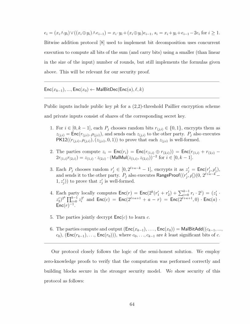
ei

= (xi

^yi

)_((xi

�yi

)^ei�1

) = xi

·yi

+(xi

�yi

)ei�1

, si

= xi

+yi

+ei�1

�2ei

for i � 1.

Bitwise addition protocol [8] used to implement bit decomposition uses concurrent

execution to compute all bits of the sum (and carry bits) using a smaller (than linear

in the size of the input) number of rounds, but still implements the formulas given

above. This will be relevant for our security proof.

Enc(xk�1

), ...,Enc(x0

) MalBitDec(Enc(a), `, k)

Public inputs include public key pk for a (2,2)-threshold Paillier encryption scheme

and private inputs consist of shares of the corresponding secret key.

1. For i 2 [0, k � 1], each Pj

chooses random bits r(j,i)

2 {0, 1}, encrypts them asz(j,i)

= Enc(r(j,i)

, ⇢(j,i)

), and sends each z(j,i)

to the other party. Pj

also executesPK12((r

(j,i)

, ⇢(j,i)

), (z(j,i)

, 0, 1)) to prove that each z(j,i)

is well-formed.

2. The parties compute zi

= Enc(ri

) = Enc(r(1,i)

� r(2,i)

)) = Enc(r(1,i)

+ r(2,i)

�2r

(1,i)

r(2,i)

) = z(1,i)

· z(2,i)

· (MalMul(z(1,i)

, z(2,i)

))�2 for i 2 [0, k � 1].

3. Each Pj

chooses random r0j

2 [0, 2`+�k � 1], encrypts it as z0j

= Enc(r0j

, ⇢0j

),and sends it to the other party. P

j

also executes RangeProof((r0j

, ⇢0i

)(0, 2`+�k�1, z0

j

)) to prove that z0j

is well-formed.

4. Each party locally computes Enc(r) = Enc(2k(r01

+ r02

) +P

k�1

i=0

ri

· 2i) = (z01

·z02

)2k

Qk�1

i=0

z2i

i

and Enc(c) = Enc(2`++1 + a � r) = Enc(2`++1, 0) · Enc(a) ·Enc(r)�1.

5. The parties jointly decrypt Enc(c) to learn c.

6. The parties compute and output (Enc(xk�1

), . . . , Enc(x0

)) = MalBitAdd((ck�1

, ...,c0

), (Enc(rk�1

), . . ., Enc(r0

))), where c0

, . . ., ck�1

are k least significant bits of c.

Our protocol closely follows the logic of the semi-honest solution. We employ

zero-knowledge proofs to verify that the computation was performed correctly and

building blocks secure in the stronger security model. We show security of this

protocol as follows:

64


rity of the building blocks, MalBitDec protocol is secure in the presence of a malicious


Proof: We prove security of MalBitDec based on Definition 2. We construct Pj

’s

view in the ideal model by building simulator Sj

, and we show it is indistinguishable

form view of Pj

in protocol’s real execution. We assume without loss of generality

that P1

is malicious, and we build simulator S1

. We can use similar proof in case P2

is malicious because MalBitDec is symmetric.

In step 1, S1

receives z(1,i)

’s, and acts as a verifier for PK12’s (extracting r(1,i)

’s).

S1

then chooses a random number c 2 {0, 1}`+ and computes

1. Enc(ri

) = Enc(xi

� ci

) = Enc(xi

) · Enc(�ci

) for i 2 [2, k � 1], where ci

denotesith least significant bit of c,

2. Enc(r1

) = Enc(x1

� c1

� c0

r0

) (if k > 1) as Enc(x1

) ·Enc(c1

) ·Enc(r0

)�1 if c0

= 1and Enc(x

1

) · Enc(c1

) otherwise, and

3. Enc(r0

) = Enc(x0

� c0

) as Enc(x0

)·Enc(0) if c0

= 0 and Enc(1�x0

) = Enc(x0

)�1 ·Enc(1) otherwise

using fresh randomness for each newly formed encryption. Note that as a result of this

computation the value that ri

takes may no longer be a bit (e.g., when xi

= 0 and ci

=

1 for i � 2). For each i 2 [0, k � 1], if r(1,i)

= 0, S1

computes z(2,i)

= Enc(ri

) · Enc(0)

and otherwise computes z(2,i)

= Enc(1 � ri

) = Enc(ri

)�1 · Enc(1) (using a freshly

formed encryption of 0 or 1). S1

then sends each z(2,i)

to P1

and simulates PK12’s as

a prover. During step 2, S1

uses MalMul’s simulator to produce P1

’s view. In step

3, S1

follows the protocol similar to P2

’s computation: it receives z01

, verifies P1

’s

RangeProof (extracting r01

), produces r02

and its corresponding ciphertext, and acts

as a prover in RangeProof. S1

skips step 4. In step 5, S1

outputs c + 2`+ � 2kr01

as

decrypted value. As a result, in the consecutive step MalBitAdd will be called on k

least significant bits of c and k ciphertexts Enc(ri

). In step 6, S1

uses MalBitAdd’s

65

simulator to interact with P1

, but introduces changes in the simulation. In particular,

S1

forces each encrypted carry bit (for i � 1) to become 0 as follows. The computation

in MalBitAdd consists of computing pi

= xi

+ yi

� 2xi

yi

and gi

= xi

yi

for each bit i

of inputs x and y, followed by computing carry bits as e0

= g0

and ei

= gi

+ pi

ei�1

for i 2 [1, k � 1] (the sum bits are computed from xi

’s, yi

’s and ei

’s as previously

described). Because one of the arguments to MalBitAdd is given in the plaintext form,

computation of pi

’s and gi

’s is local and beyond the simulator’s control. Computing

each ei

(for i � 1), however, involves a call to MalMul, where we instruct S1

to deviate

from MalMul’s simulation. In particular, when S1

simulates P1

’s view during a call

to MalMul(Enc(pi

),Enc(ei�1

)), instead of setting z2

to Enc(pi

ei�1

)�1Enc(ei�1

)w�r1 in

step 2 as MalMul’s simulation prescribes, S1

sets z2

to Enc(gi

)Enc(ei�1

)w�r1 . This

will cause the product to evaluate to �gi

and consequently result in ei

being 0 for

each i � 1. (We note that ei

’s are not computed sequentially in BitAdd to reduce the

number of rounds, but this does not a↵ect how we instruct the simulator to work.)

The remaining multiplications are simulated according to MalMul’s simulator.

Now we show that P1

’s output at the end of simulation is computed correctly.

During the simulation, S1

sets each r2,i

such that r(2,i)

= ri

� r(1,i)

and consequently

ri

= r(1,i)

� r(2,i)

, where ri

= xi

� ci

for i � 2, r0

= x0

� c0

, and r1

= x1

� c1

� c0

r0

.

Then because k least significant bits of c = c + 2`+ � 2kr01

correspond to k least

significant bits c, MalBitAdd is going to be called on arguments (ck�1

, . . ., c0

) and

(Enc(rk�1

), . . .,Enc(r0

)). As part of MalBitAdd P1

then computes the carry bit e0

as

c0

r0

, while all other carry bits ei

for i � 1 will be forced to be 0 (by changing what

MalMul returns) as described earlier. Recall that the output bits of MalBitAdd (and

the output bits of BitDec are computed as s0

= c0

+r0

�2e0

and si

= ci

+ri

+ei�1

�2ei

.

Because all ei

= 0 for i � 1, but e0

can be set to 1, we obtain that

1. s0

= c0

+ r0

� 2c0

r0

= c0

� r0

= x0

as required;

2. s1

is supposed to be computed as s1

= c1

+ r1

+ e0

� 2e1

, but we instead have

66

s1

= c1

+ r1

+ e0

. Recall, however, that r1

was set to r1

= x1

� c1

� c0

r0

=x1

� c1

� e0

, which gives us s1

= c1

+ x1

� c1

� e0

+ e0

= x1

as required;

3. si

for i � 2 becomes ci

+ ri

as a result of S1

’s simulation. Because ri

was set toxi

� ci

, we obtain that si

= ci

+ xi

� ci

= xi

as required as well.

The last piece that we wanted to demonstrate is that P1

will compute each ri

according to the value that S1

expects even when ri

is not a bit (which would be a vi-

olation of the real protocol execution). During the simulation, r0

is always computed

as a bit, r1

may take values �1 and �2 (in addition to 0 and 1), and ri

may take

value �1 (in addition to 0 and 1). S1

sets each r2,i

as XOR of ri

and r(1,i)

using the

formula ri

+r(1,i)

�2ri

r(1,i)

(i.e., r(2,i)

is either ri

or 1�ri

based on the value of the bit

r(1,i)

) and later P1

computes ri

= r(1,i)

+ r(2,i)

� 2r(1,i)

r(2,i)

. The crucial fact that we

are using here is that ri

� r(1,i)

� r(1,i)

= ri

for any value of ri

as long as r(1,i)

is a bit.

In other words, during the simulation r(2,i)

= ri

and then ri

= r(2,i)

when r(1,i)

= 0;

and r(2,1)

= 1 � ri

and then ri

= 1 � r(2,i)

= 1 � (1 � ri

) = ri

when r(1,i)

= 1. We

conclude that P1

learns the correct (encrypted) output bits x0

, . . ., xk�1

as a result of

this simulation.



’s view in the

hybrid model, we need to show the plaintext value the simulator produces in step 5 is

indistinguishable from the value c in real execution (as the remaining building blocks

have been shown to guarantee indistinguishability and all encrypted values achieve

indistinguishability as well). Recall that in the real protocol execution c is formed as

2`++1�r+x = 2`++1�2k(r01

+r02

)�P

k�1

i=0

2iri

+x, while in the simulation S1

outputs

c = c + 2`+k � 2kr01

. Let c = 2`+ � 2kr02

�P

k�1

i=0

. Because no information about r02

and ri

’s is available to P1

, c in the simulation and 2`+ � 2kr02

�P

k�1

i=0

during real

execution are distributed identically. We obtain that during the real execution P1

observes 2`++1�r+x, while during the simulation P1

observes 2`++1�r. These two

values are statistically indistinguishable using statistical security parameter . Note

that we have to take the value of r01

into account when forming c during the simulation

67

to ensure that c that the simulator outputs falls in the correct range (according to P1

’s

knowledge of r01

). Lastly, we note that both during the simulation and real execution

the computation aborts only when a malicious party fails to correctly complete ZKPKs

as the prover. Therefore, simulated and real views are indistinguishable. 2

4.6.2.7 Performance of the New Building Blocks

With MalMul, MalLT, RangeProof, MalTruncPR, MalInv, MalPreMul, MalBitDec,

and previously mentioned prior work, we achieve security of the HMM and GMM

protocols in the malicious model in the homomorphic encryption setting. The com-

plexities of the new protocols are provided in Table 4.1.

68

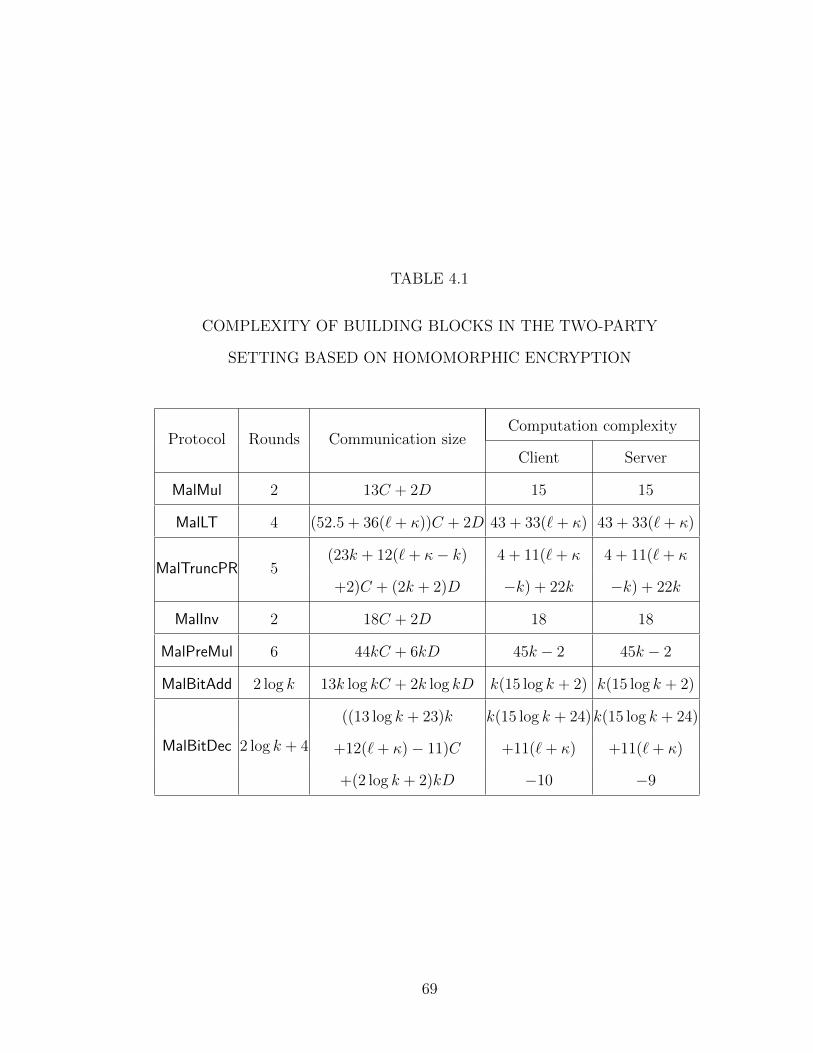
TABLE 4.1

COMPLEXITY OF BUILDING BLOCKS IN THE TWO-PARTY

SETTING BASED ON HOMOMORPHIC ENCRYPTION

Protocol Rounds Communication sizeComputation complexity

Client Server

MalMul 2 13C + 2D 15 15

MalLT 4 (52.5 + 36(`+ ))C + 2D 43 + 33(`+ ) 43 + 33(`+ )

MalTruncPR 5(23k + 12(`+ � k) 4 + 11(`+ 4 + 11(`+

+2)C + (2k + 2)D �k) + 22k �k) + 22k

MalInv 2 18C + 2D 18 18

MalPreMul 6 44kC + 6kD 45k � 2 45k � 2

MalBitAdd 2 log k 13k log kC + 2k log kD k(15 log k + 2) k(15 log k + 2)

MalBitDec 2 log k + 4

((13 log k + 23)k k(15 log k + 24)k(15 log k + 24)

+12(`+ )� 11)C +11(`+ ) +11(`+ )

+(2 log k + 2)kD �10 �9

69

CHAPTER 5

DNA COMPUTATIONS

Computation based on genomic data is becoming increasingly popular today, be it

for medical or other purposes such as ancestry or paternity testing. Non-medical uses

of genomic data in a computation often take place in a server-mediated setting where

the server o↵ers the ability for joint genomic testing between the users. Undeniably,

genomic data is highly sensitive, which in contrast to other biometry types, discloses

a plethora of information not only about the data owner, but also about his or her

relatives. Thus, there is an urgent need to protect genomic data, especially when it

is used in computation for what we call as recreational non-health-related purposes.

Towards this goal, in this work we put forward a framework for server-aided secure

two-party computation with the security model motivated by genomic applications.

In this chapter, we talk about motivation and contributions in Sections 5.1 and

5.2. Section 5.3 provides necessary information about the selected genomic tests.

Sections 5.4 and 5.5 describe the security model and our proposed solutions. Then

Section 5.6 provides private genomic computations based on the proposed protocols.

Experimental evaluation of our secure genomic tests is given in Section 5.7.

5.1 Motivation

The motivation for this work comes from rapidly expanding availability and use of

genomic data in a variety of applications and the need to protect such highly sensitive

data from potential abuse. The cost of sequencing one’s genome has dramatically

decreased in the recent years and is continuing to decrease, which makes such data

70

more readily available for a number of applications. Examples of such applications

include:

• Personalized medicine, where genomic tests are performed prior to prescribinga drug treatment to ensure its e↵ectiveness;

• Paternity testing, which use DNA data to determine whether one individual isthe father of another individual;

• Genomic compatibility tests, which allow potential or current partners to de-termine whether their future children are likely to inherit genetic conditions;

• Determining ancestry and building genealogical trees by examining DNA dataof many individuals and finding relationships among specific individuals.

Genomic tests are increasingly used for medical purposes to ensure the best treat-

ment. A number of services for what we call the “leisure” use of DNA data has

flourished as well (examples are [1–3, 66]) allowing for various forms of comparing

DNA data, be it for the purposes of building ancestry trees, genomic compatibility

or other.

It is clear that DNA is highly sensitive and needs to be protected from unintended

uses. It can be viewed as being even more sensitive than other types of biometry as-

sociated with an individual, as not only it allows for unique identification of an indi-

vidual, but it also allows to learn a plethora of information about the individual such

as predisposition to medical conditions and relatives of the individual thus exposing

information about others as well. Furthermore, our understanding of genomes is con-

tinuously growing and exposure of DNA data now can lead to consequences which

we cannot even anticipate today.

5.2 Contributions

The first observation we make about such types of genomic computation is that

they are normally facilitated by some service or third party. For example, both ances-

try and gene-based matchmaking web sites allow participants to interact with each

71

other through the service provider. Such service providers serve as a natural point

for aiding the individuals with private computation on their sensitive genomic data.

In some prior publications on genomic computation (e.g., [20]), it is assumed that

computation such as paternity testing or genetic compatibility is run between a client

and a server, while we believe that it is more natural to assume that such compu-

tation is carried out by two individuals through some third-party service provider.

Thus, in this work we look at private genomic computation in the light of server-

mediated setting and utilize the server to lower the cost of the computation for the

participants. Throughout this chapter, we will refer to the participants as Alice (A),

Bob (B), and the server (S).

From the security point of view, participants in a protocol that securely evalu-

ates a function are normally assumed to be either semi-honest or malicious. In our

application domain, we may want to distinguish between di↵erent security settings

depending on how well Alice and Bob know each other. For example, if Alice and

Bob are relatives and would like to know how closely they are related (i.e., how

closely their genealogical trees overlap), it would be reasonable to assume that they

will not deviate from the prescribed computation in the attempt to cheat each other,

i.e., they can be assumed to be semi-honest. On the other hand, if Alice and Bob

meet each other through a matchmaking web site and do know each other well, it

is reasonable for them to be cautious and engage in a protocol that ensures security

(i.e., correctness and privacy) even in presence of malicious participants. The server

can typically be expected not to deviate from its prescribed behavior, as it would lose

its reputation and consequently revenue if any attempts at cheating become known.

If, however, adding protection against server’s malicious actions is not very costly, it

can also be meaningful to assume a stronger security model.

Another important consideration from a security point of view is enforcing correct

inputs to be entered in the computation when, for instance, the inputs are certified

72

by some authority. This requirement is outside the traditional security model for

secure multi-party computation (even in presence of fully malicious actors), and to

the best of our knowledge certified inputs were previously considered only for specific

functionalities such as private set intersection [42, 55] or anonymous credentials and

certification [43], but not for general secure function evaluation. We bring this up in

the context of genomic computation because for certain types of genomic computation

it is very easy for one participant to modify his inputs and learn sensitive information

about genetic conditions of the other participant. For example, genetic compatibility

tests evaluate the possibility of two potential or existing partners to determine the

possibility of transmitting to their children a genetic disease. Such possibility is

present when both partners are (silent) carriers of that disease (see Section 5.3 for

more detail). Then if the partners can each separately evaluate their DNA for a

fingerprint of specific disease, the joint computation can consist of a simple AND of

the bits provided by both parties (for one or more conditions). Now if a malicious

participant sets all of his input bits to 1 and the outcome is positive, the participant

learns that the other party is a carrier for a specific medical condition (or at least one

condition from the set of specific conditions). We thus would like prevent malicious

participants from modifying their inputs used in genomic computation in cases such

data can be certified by certification authorities such as medical facilities.

The aspect of secure computation related to security properties that we treat in

this work is fairness. In particular, it is known that full fairness cannot be achieved

in the case of two-party computation in the malicious security model [49], but it

becomes possible in the server-aided setting. Fairness has been considered in the

server-aided literature in the past [71, 79] and achieving fairness only adds minimal

overhead to the solutions in the settings we consider.

Thus, we categorize our contributions in two main groups: (i) results applicable

to general secure function evaluation and (ii) results specific to genomic tests, both

73

of which we consequently describe. All constructions rely on garbled circuit evalua-

tion typically used in the two-party setting, but which we adopt to the three-party

computation between the server and two users. We present from the simplest and

enabling most e�cient solutions to the most complex with added security guarantees.

1. Our most e�cient solution is designed for the setting where A and B are semi-honest and S can be malicious (as in the ancestry testing scenario). In thissetting, the solution consists of a single circuit garbling and single evaluation ofthe garbled circuit and the need for oblivious transfer is eliminated all together.

2. Our second solution works in the setting where A and B can be malicious, but Sis semi-honest (applicable to the paternity test) and achieves fairness for A andB. In this solution, the combined work for all participants is approximately thesame as the combined work of two participants in a two-party protocol basedon garbled circuit in presence of semi-honest participants only.

3. Our last solution strengthens the model of malicious A and B with input cer-tification (applicable to the genomic compatibility test). In more detail, inaddition to being able to behave arbitrarily, A and B may maliciously modifytheir true inputs. To combat this, the function f being evaluated is modifiedto mark any suitable subset of the inputs as requiring certification. At thetime of secure function evaluation, A and B have to prove that the inputs thatthey enter in the protocol are identical to the values signed by a trusted au-thority (a medical facility that performs genomic tests in our case). Achievingthis involves the use of additional tools such as a signature scheme and ZKPKs.Handling of the remaining inputs and the rest of the computation is not a↵ectedby the shift to a stronger security model.

All of our constructions o↵er conceptual simplicity and at the same time achieve

highly attractive performance. To the best of our knowledge, the strongest of our

models which enforces correctness of the inputs have not been treated in the context

of general secure multi-party computation and computation based on garbled circuit

in particular. Despite the drastic di↵erences in the techniques for garbled circuit eval-

uation and data certification, we show how they can be integrated by using oblivious

transfer as the connecting point or even when oblivious transfer is not used.

Based on the solutions described above, we build implementations of three genetic

tests, namely, genetic common ancestry, paternity, and genetic compatibility tests.

74

Each test uses a di↵erent security setting. We show through experimental results that

each of the implemented tests is e�cient with the worst runtime being on the order

of a couple of seconds. The performance favorably compares to the state of the art

(as detailed in Section 5.7), in some cases achieving orders of magnitude performance

improvement over existing solutions.

5.3 Genomic Testing

Genomes represent complete hereditary information of an individual. Information

extracted from one’s genome can take di↵erent forms. One type is called Single Nu-

cleotide Polymorphisms (SNPs), each of which corresponds to a well known variation

in a single nucleotide.1 Because SNP mutations are often associated with how one

develops diseases and responds to treatments, they are commonly used in genetic

disease and disorder testing. The same set of SNPs (i.e., nucleotides in the same po-

sitions) would be extracted for each individual, but the values associated with each

SNP di↵er from one individual to another. Normally each SNP is referenced by a spe-

cific index and its value in a individual is represented as a bit, while representations

consisting of 3 values 0, 1, 2 are used as well.

Another type of data extracted from a genome is based on Short Tandem Repeats

(STRs). STRs occur when a short region consisting of two or more nucleotides is

repeated and the occurrences are adjacent to each other. Unrelated individuals are

likely to have a di↵erent number of repeats of a given STR sequence in certain regions

in their DNA and thus STRs are often used for identity testing or testing between

close relatives (such as paternity testing).

Paternity test. This test is normally done based on STRs. STR profile of a per-

son consists of an ordered sequence of N 2-element sets S = h{x1,1

, x1,2

}, {x2,1

, x2,2

},

1A nucleotide can be viewed as a simple unit represented by a letter A, C, G, or T.

75

. . ., {xN,1

, xN,2

}i, where each value corresponds to the number of repeats of a specific

STR sequence at specific locations in the genome. For each STR i, one of xi,1

and

xi,2

is inherited from the mother and the other from the father.

Thus in the paternity test with a single parent, there are two STR profiles S =

h{xi,1

, xi,2

}i and S 0 = h{x0i,1

, x0i,2

}i corresponding to the child and the contested father,

respectively. To determine whether S 0 corresponds to the father’s child, the test

computes whether for each i the child’s set {xi,1

, xi,2

} contains (at least) one element

from the contested father’s set {x0i,1

, x0i,2

}. In other words, the test corresponds to

the computation

N^

i=1

[{x1,i

, x2,i

} \ {x01,i

, x02,i

} 6= ;] = True (5.1)

when testing with both parents is performed, for each STR i one of xi,1

and xi,2

must

appear in the mother’s set and the other in the father’s set. Using both parents’

profiles in the computation increases the accuracy of the test, but even the single

parent test has high accuracy for a small number N of well-chosen STRs (e.g., the

US CODIS system utilizes N = 13, while the European SGM Plus identification

method uses N = 10).

Genetic compatibility test. While there is a variety of genetic tests that can

be used for several purposes, we concentrate on the genetic compatibility test where

potential (or existing) partners would like to determine the possibility of transmitting

to their children a genetic disease with Mendelian inheritance. In particular, if a

specific mutation occurs in one allele2 (called minor), it often has no impact on one’s

quality of life, but when the mutation occurs in both alleles (called major), the disease

manifests itself in severe forms. If both partners silently carry a single mutation, they

have a noticeable chance of conceiving a child carrying the major variety. Thus, a

2An allele is one of the alternative versions of a gene at a given location.

76

genetic compatibility test for a given genetic disease would test for the presence of

minor mutations in both partners.

The current practice for screening for most genetic diseases consists of testing one

SNP in a specific gene. It is, however, expected that in the future tests for more

complex diseases (that involve multiple genes and mutations) will become available.

Thus, a genetic disease can be characterized by a set of SNP indices and the corre-

sponding values (i1

, b1

), . . ., (it

, bt

), where ij

is the SNP index and bj

2 {0, 1} is the

value it takes. Then if the same values are found in the appropriate SNPs of an

individual, we assume that the individual is tested as positive (i.e., the individual is

the disease carrier). If both partners test as positive, then the outcome of the genetic

compatibility test will be treated as positive and otherwise it is negative.

Ancestry test. There are a number of tests that allow for various forms of

ancestry testing, for example, tests using Y-chromosome STRs (applicable to males

only), mitochondrial DNA (mtDNA) test on the maternal line, and more general

SNP-based tests for common ancestry or one’s genealogy. Many such tests are not

standardized and in addition current ancestry and genealogy service providers often

use proprietary algorithms. The advantage of STR-based tests is that normally only

a relatively small number of STRs are tested, while SNP-based tests often utilize

a large number of (or even all available) SNPs, but more distant ancestry can be

learned from SNP-based tests. For improved accuracy it is also possible to perform

one type of testing after the other. In either case, to determine the most recent

common ancestor between two individuals, the markers from the two individuals

are compared and their number determines how closely the individuals are related.

Certain tests such as determining geographical regions of one’s ancestors normally

require genetic data from many individuals.

77

5.4 Security Model

We formulate security using the standard ideal/real model for secure multi-party

computation, where the view of any adversary in the real protocol execution should

be indistinguishable from its view in the ideal model where a trusted party (TP)

evaluates the function. Because the server does not contribute any input, it is mean-

ingful to consider that either A or B is honest since the goal is to protect the honest

party.

We are primarily interested in the setting where the server is semi-honest, but

parties A and B may either be semi-honest or fully malicious. Thus, we target security

models where S complies with the computation, with the exception of the first setting

of semi-honest A and B, where we get security in the presence of a malicious server

for free. We similarly assume that the server will not collude with users (putting its

reputation at risk) or let users a↵ect its operation.

We obtain security settings where (1) A and B can be corrupted by a semi-honest

adversary, while S can act on behalf of a fully malicious adversary and (2) A and B

can be malicious, but the server is semi-honest. Because we assume that the parties

(or the adversaries who corrupt them) do not collude, at any given point of time

there might be multiple adversaries, but they are independent of each other. This is

similar to the setting used in [78, 79]. We note that based on the security settings

listed above, at most one adversary would be fully malicious. In other words, if in (2)

A is malicious, the goal is to protect B who is assumed to not be malicious and S is

semi-honest, while in (1) S can be malicious, while A and B are semi-honest. Kamara

et al. [78], however, show that in the presence of non-cooperating adversaries who

corrupt only one party, showing security can be reduced to showing that the protocol

is secure in the presence of semi-honest adversaries only, followed by proving for each

malicious adversary Ai

that the solution is secure in the presence of Ai

when all other

parties are honest. More precisely, we rely on the following lemma:

78

Lemma 1 ([78]) If a multi-party protocol ⇧ between n parties P1

, . . . , Pnp

securely

computes f in the presence of (i) independent and semi-honest adversaries and (ii) a

malicious Ai

and honest {Aj

}j 6=i

, then ⇧ is also secure in the presence of an adversary

Ai

that is non-cooperative with respect to all other semi-honest adversaries.

This implies that in our setting (2) a solution secure in the presence of malicious

A or B will also remain secure when A and B are corrupted by two independent

malicious adversaries.

To model fairness, we modify the behavior of the TP in the ideal model to send

? to all parties if any party chooses to abort (note that fairness is only applicable

to A and B). We assume that A and B learn the result of evaluation of a predefined

function f that takes input x1

from A and x2

from B, and the server learns nothing.

Because our primary motivation is genomic computation, we consider single-output

functions, i.e., both A and B learn f(x1

, x2

) (but two of our constructions support

functions where A’s and B’s outputs di↵er and the remaining protocol in the present

form loses only fairness).

Execution in the real model. The execution of protocol ⇧ in the real model

takes place between parties A, B, S and a subset of adversaries AA

, AB

, AS

who can

corrupt the corresponding party. LetA denote the set of adversaries present in a given

protocol execution. A and B receive their respective inputs xi

and a set of random

coins ri

, while S receives only a set of random coins r3

. All parties also receive security

parameter 1. Each adversary receives all information that the party it corrupted

has and a malicious adversary can also instruct the corresponding corrupted party

to behave in a certain way. For each AX

2 A, let VIEW⇧,A

X

denote the view of the

adversary AX

at the end of an execution of ⇧. Also let OUThon

⇧,A denote the output

of the honest parties (if any) after the same execution of the protocol. Then for each

AX

2 A, we define the partial output of a real-model execution of ⇧ between A, B,

S in the presence of A by REAL⇧,A

X

(, x1

, x2

, r1

, r2

, r3

)def

= VIEW⇧,A

X

[OUThon

⇧,A.

79

Execution in the ideal model. In the ideal model, all parties interact with

a TP party who evaluates f . Similar to the real model, the execution begins with

A and B receiving their respective inputs xi

and each party (A, B, and S) receiving

security parameter 1. Each honest (semi-honest) party sends to the TP x0i

= xi

and each malicious party can send an arbitrary value x0i

to the TP. If x1

or x2

is

equal to ? (empty) or if the TP receives an abort message, the TP returns ? to all

participants. Otherwise, A and B receive f(x01

, x02

). Let OUThon

f,A denote the output

returned by the TP to the honest parties and let OUTf,A

X

denote the output that

corrupted party AX

2 A produces based on an arbitrary function of its view. For

each AX

2 A, the partial output of an ideal-model execution of f between A, B, S

in the presence of A is denoted by IDEALf,A

X

(, x1

, x2

)def

= OUTf,A

X

[OUThon

f,A.

Definition 3 (Security) A three-party protocol ⇧ between A, B, and S securely

computes f if for all sets of probabilistic polynomial time (PPT) adversaries A in

the real model, for all xi

and 2 Z, there exists a PPT transformation SX

for each

AX

2 A such that REAL⇧,A

X

(, x1

, x2

, r1

, r2

, r3

)c⇡ IDEAL

f,SX

(, x1

, x2

), where each

ri

is chosen uniformly at random andc⇡ denotes computational indistinguishability.

To model the setting where some of the inputs of A and/or B are certified, we

augment the function f to be executed with the specification of what inputs are to

be certified and two additional inputs y1

and y2

that provide certification for A’s and

B’s inputs, respectively. Then in the ideal model execution, the TP will be charged

with additionally receiving yi

’s. If the TP does not receive all inputs or if upon

receiving all inputs some inputs requiring certification do not verify, it sends ? to

all parties. In the real model execution, verification of certified inputs is built into ⇧

and besides using two additional inputs y1

and y2

the specification of the execution

remains unchanged.

Definition 4 (Security with certified inputs) A three-party protocol ⇧ between

A, B, and S securely computes f if for all sets of PPT adversaries A in the real model,

80

for all xi

, yi

, and 2 Z, there exists a PPT transformation SX

for each AX

2 A

such that REAL⇧,A

X

(, x1

, x2

, y1

, y2

, r1

, r2

, r3

)c⇡ IDEAL

f,SX

(, x1

, x2

, y1

, y2

), where

each ri

is chosen uniformly at random.

5.5 Server-Aided Computation

In this section we detail our solutions for server-aided two party computation

based on garbled circuit. The current description is general and can be applied to

any function f . In Section 5.6 we describe how these constructions can be applied to

genomic tests to result in fast performance. For the rest of this chapter, t1

(t2

) shows

the number of A’s (B’s) input bits, and t3

represents the number of output bits.

5.5.1 Semi-Honest A and B, Malicious S

Our first security setting is where A and B are semi-honest and S can be malicious.

The main intuition behind the solution is that when A and B can be assumed to be

semi-honest and a solution based on garbled circuit evaluation is used, we will charge

S with the task of evaluating a garbled circuit. That is, security is maintained in the

presence of malicious server because garbled circuit evaluation techniques are secure

in the presence of a malicious evaluator. Next, we notice that if A and B jointly form

garbled representation of the circuit for the function f they would like to evaluate,

both of them can have access to the pairs of labels (`0i

, `1i

) corresponding to the

input wires. Thus, they can simply send the appropriate label `bi

to S for evaluation

purposes for their value of the input bit b for each input wire. This eliminates the

need for OT and results in a solution that outperforms a garbled circuit protocol in

the presence of only semi-honest participants. The same idea was sketched in [58]

(with the di↵erence that S was to learn the output). The use of a pseudo-random

function PRF : {0, 1}⇥{0, 1}⇤ ! {0, 1} with security parameter for deriving wire

labels in the scheme is as in [97].

81

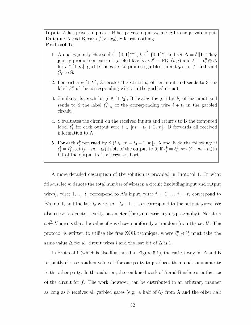
Input: A has private input x1

, B has private input x2

, and S has no private input.Output: A and B learn f(x

1

, x2

), S learns nothing.Protocol 1:

1. A and B jointly choose �R {0, 1}�1, k

R {0, 1}, and set � = �||1. Theyjointly produce m pairs of garbled labels as `0

i

= PRF(k, i) and `1i

= `0i

��for i 2 [1,m], garble the gates to produce garbled circuit G

f

for f , and sendGf

to S.

2. For each i 2 [1, t1

], A locates the ith bit bi

of her input and sends to S thelabel `bi

i

of the corresponding wire i in the garbled circuit.

3. Similarly, for each bit j 2 [1, t2

], B locates the jth bit bj

of his input and

sends to S the label `b

j

i+t1of the corresponding wire i + t

1

in the garbledcircuit.

4. S evaluates the circuit on the received inputs and returns to B the computedlabel `b

i

for each output wire i 2 [m � t3

+ 1,m]. B forwards all receivedinformation to A.

5. For each `bi

returned by S (i 2 [m� t3

+ 1,m]), A and B do the following: if`bi

= `0i

, set (i�m+ t3

)th bit of the output to 0, if `bi

= `1i

, set (i�m+ t3

)thbit of the output to 1, otherwise abort.

A more detailed description of the solution is provided in Protocol 1. In what

follows, letm denote the total number of wires in a circuit (including input and output

wires), wires 1, . . ., t1

correspond to A’s input, wires t1

+ 1, . . ., t1

+ t2

correspond to

B’s input, and the last t3

wires m� t3

+1, . . .,m correspond to the output wires. We

also use to denote security parameter (for symmetric key cryptography). Notation

aR U means that the value of a is chosen uniformly at random from the set U . The

protocol is written to utilize the free XOR technique, where `0i

� `1i

must take the

same value � for all circuit wires i and the last bit of � is 1.

In Protocol 1 (which is also illustrated in Figure 5.1), the easiest way for A and B

to jointly choose random values is for one party to produces them and communicate

to the other party. In this solution, the combined work of A and B is linear in the size

of the circuit for f . The work, however, can be distributed in an arbitrary manner

as long as S receives all garbled gates (e.g., a half of Gf

from A and the other half

82

Figure 5.1. Illustration of Protocol 1 with weak A (who contributes onlygarbled labels for her input wires to the computation).

from B). Besides equally splitting the work of circuit garbling between the parties,

an alternative possibility is to let the weaker party (e.g., a mobile phone user) to do

work sublinear in the circuit size. Let A be a weak client, who delegates as much

work as possible to B. Then B generates the entire garbled circuit and sends it to S,

while A will only need to create t1

label pairs corresponding to her input, to be used

in step 2 of the protocol. Upon completion of the result, A learns the output from

B (i.e., there is no need for A to know labels for the output wires). Thus, the work

and communication of the weaker client is only linear in the input and output sizes.

Security of this solution can be stated as follows:

Theorem 7 Protocol 1 fairly and securely evaluates function f in the presence of

semi-honest A and B and malicious S.

Proof: Fairness is achieved based on the fact that A and B are semi-honest. This

means that if B ever learns any output, he will share (the part of) the output he

83

receives with the other party. Thus, either both of them learn the (possibly partial)

output or neither party learns the output.

To show simulation-based security, we build three independent simulators SS

, SB

,

and SA

for three independent adversaries AS

, AB

, and AA

, respectively. Note that

AS

can act in an arbitrary way while AB

and AA

are semi-honest.

We first consider a simulator SS

that communicates with malicious AS

pretending

to be A and B (without access to their private inputs) in such a way that SS

is unable

to distinguish it from an execution in the real model. SS

proceeds by garbling a circuit

corresponding to f and sending it to AS

. For each wire i 2 [1, t1

+ t2

], SS

sends label

`bii

for a randomly chosen bit bi

. If AS

does not abort, SS

obtains from AS

a set of

labels corresponding to the output wires. It is easy to see that the view simulated

by SS

is indistinguishable from the view of AS

in the real model execution (since the

view of garbled circuit evaluator is independent of the input on which the circuit is

evaluated). Note that the simulator can safely use random inputs because S is not

entitled to receiving any information about the result of function evaluation.

We next consider a simulator SB

for semi-honest AB

. Note that AB

’s advantage

is maximized when B constructs the entire garbled circuit (or simply knows the

random label pairs for all wires of the circuit), which we assume is the case. After

AB

constructs the circuit and forms the input labels according to x2

, SB

queries the

trusted party and obtains B’s output f(x1

, x2

). SB

then extracts from AB

’s view

the output labels corresponding to the received output f(x1

, x2

) from the set of the

label pairs for the output wires and sends them to AB

. SB

also receives assembled

f(x1

, x2

) from AB

destined to A. This view is the same as the view of AB

in the real

model execution given the same set of random coins.

A simulator for AA

is built analogously with the exception that AA

receives (from

SA

) f(x1

, x2

) directly instead of learning labels for the output wires. 2

84

5.5.2 Semi-Honest S, Malicious A and B

To maintain e�ciency of the previous solution by avoiding the cost of OT, we

might want to preserve the high-level structure of the computation in the first solu-

tion. Now, however, because A and B can be malicious, neither of them can rely on

the other party in garbling the circuit correctly. To address this, each of A and B

may garble their own circuit for f , send it to S, and S will be in charge of evaluating

both of them and performing a consistency check on the results (without learning

the output). With this solution, A would create label pairs for her input bits/wires

for both garbled circuit and communicate one set of pairs to B who uses them in

constructing his circuit. What this achieves is that now A can directly send to S

the labels corresponding to her input bits for circuit evaluation for both circuits. B

performs identical operations. There is still no need to perform OT, but two secu-

rity issues arise: (1) A and B must be forced to provide consistent inputs into both

circuits and (2) regardless of whether the parties learn the output (e.g., whether the

computation is aborted or not), a malicious party can learn one bit of information

about the other party’s input (by constructing a circuit that does not correspond to

f) [75, 95]. While the first issue can be inexpensively addressed using the solution

of [86] (which works in the presence of malicious users and semi-honest server), the

second issue will still stand with this structure of the computation.

Instead of allowing for (1-bit) information leakage about private inputs, we change

the way the computation takes place. If we now let the server garble the circuit and

each of the remaining parties evaluate a copy of it, the need for OT (for both A and

B’s inputs) arises. We, however, were able to eliminate the use of OT for one of A and

B and construct a solution that has about the same cost as a single garbled circuit

solution in the semi-honest model. At a high-level, it proceeds as follows: A creates

garbled label pairs (`0i

, `1i

) for the wires corresponding to her inputs only and sends

them to S. S uses the pairs to construct a garbled circuit for f and sends it to B. S

85

and B engage in OT, at the end of which B learns labels corresponding to his input

bits. Also, A sends to B the labels corresponding to her input bits, which allows B

to evaluate the circuit. We note that because A may act maliciously, she might send

to B incorrect labels, which will result in B’s inability to evaluate the circuit. This,

however, is equivalent to A aborting the protocol. In either case, neither A nor B

learn any output and the solution achieves fairness. Similarly, if B does not perform

circuit evaluation correctly, neither party learns the output.

The next issue that needs to to addressed is that of fairly learning the output.

We note that S cannot simply send the label pairs for the output wires to A and B

as this would allow B to learn the output and deny A of this knowledge. Instead,

upon completion of garbled circuit evaluation, B sends the computed labels to A.

With the help of S, A verifies that the labels A possesses are indeed valid labels for

the output wires without learning the meaning of the output. Once A is satisfied,

she notifies S who sends the label pairs to A and B, both of whom can interpret and

learn the result. We note that malicious A can report failure to S even if verification

of the validity of the output labels received from B was successful. Once again, this is

equivalent to A aborting the protocol, in which case neither party learns the output

and fairness is maintained.

Our solution is given as Protocol 2 below (which is also illustrated in Figure 5.2)

and uses a hash function H : {0, 1}⇤ ! {0, 1} that we treat as a random oracle. We

show security of this solution in a hybrid model where the parties are given access to

a trusted entity computing OT.


malicious A or B and semi-honest S in the hybrid model with ideal implementation

of OT and where H is modeled as a random oracle.

Proof: As before, we start by showing fairness and then proceed with security. The

only way for A or B to learn any output is when A is satisfied with the verification

86


, B has private input x2

, and S has no private input.Output: A and B learn f(x

1

, x2


1. S chooses �R! {0, 1}�1, k

1

R! {0, 1}, k2

R! {0, 1} and sets � = �||1. Ssends � and k

1

to A.

2. S computes wire labels `0i

= PRF(k1

, i) for i 2 [1, t1

], `0i

= PRF(k2

, i� t1

) fori 2 [t

1

+ 1,m], and sets `1i

= `0i

�� for i 2 [1,m]. S then constructs garbledgates G

f

and sends Gf

to B.

3. S and B engage in t2

instances of 1-out-of-2 OT, where S assumes the roleof the sender and uses t

2

label pairs (`0t1+i

, `1t1+i

) for i 2 [1, t2

] correspondingto B’s input wires as its input and B assumes the role of the receiver anduses his t

2

input bits bi

as the input into the protocol. As the result of theinteraction, B learns garbled labels `bi

t1+i

for i 2 [1, t2

].

4. A computes labels `0i

= PRF(k1

, i) for i 2 [1, t1

] and sends to B `bii

for herinput bits b

i

, where `1i

= `0i

�� for any bi

= 1.

5. After receiving the labels for his own and A’s input, B evaluates the circuit,learns the output labels `bi

i

for i 2 [m� t3

+ 1,m] and sends them to A.

6. A requests from S output verification constructed as follows: For each outputwire i, S computes H(`0

i

), H(`1i

), randomly permutes the tuple, and sends itto A.

7. For each label `i

received from B in step 5, A computes H(`i

) and checkswhether the computed value appear among H(`b

i

), H(`1�b

i

) received from Sin step 6. If the check succeeds for all output wires, A notifies S of success

8. Upon receiving confirmation of success from A, S sends (`0i

, `1i

) for all outputwires i to A and B, who recover the output.

87

Figure 5.2. Illustration of Protocol 2.

of the output labels she received from B. Recall that each received label ì

is checked

against H(`bi

), H(`1�b

i

) for some bit b, where H is a collision-resistant hash function.

The probability that this check succeeds for some ì

that is not equal to `0i

or `1i

is

negligible. Thus, A is guaranteed to possess the result of garbled circuit evaluation,

at which point both parties are given access to the output.

We next construct simulators for all of the (independent) adversaries AA

, AB

,

and AS

. We start with a simulator SA

for malicious AA

. SA

runs AA

and simulates

the remaining parties. AA

produces t1

random labels `0i

and sends them to SA

, while

SA

chooses � and sends it to AA

. If at least one label is of an incorrect bitlength, SA

aborts. If SA

did not abort, AA

sends t1

labels to SA

. If the ith label sent by AA

does

not correspond to one of the labels in the ith pair of labels (`0i

, `0i

��) corresponding

to AA

’s inputs, SA

aborts. If SA

did not abort, it interprets the meaning of the

input labels received from AA

and stores the input as x01

. At some point SA

creates a

random label ì

for each bit of the output and sends them to AA

. Upon AA

’s request,

88

SA

also chooses another random label `0i

for each bit of the output. For each bit i of

the output, SA

sends to AA

the pair H(ì

), H(`0i

) in a randomly permuted order. If

AA

notifies SA

of successful verification of the output labels, SA

queries the trusted

party for the output f(x01

, x2

). For each ith bit bi

of the output, if bi

= 0, SA

sends

to AA

the pair (ì

, `0i

), otherwise, SA

sends the pair (`0i

, ì

).

Now we examine the view of AA

in the real and ideal model executions and cor-

rectness of the output. After receiving the label pairs from AA

, SA

performs the

same checks on them as S would and thus both would abort in the same circum-

stances. Similarly, if AA

provides malformed labels for circuit evaluation, SA

will

immediately detect this in the ideal model and abort, while B in the real world will

be unable to evaluate the circuit and also abort. Otherwise, in both cases the func-

tion will be correctly evaluated on the input provided by AA

and B’s input. In the

remaining interaction, AA

sees only random values, which in the ideal world are con-

structed consistently with AA

’s view in the real model execution. Thus, AA

’s view

is indistinguishable in the two executions.

Let us now consider malicious AB

, for which we construct simulator SB

in the

ideal model execution who simulates correct behavior of A and S. First, SB

simulates

the OT. It records the input bits used by AB

during the simulation, which it stores as

x02

and returns t2

random labels to AB

. SB

also sends another set of t1

random labels

to SB

. SB

queries the trusted party for AB

’s output f(x1

, x02

) and chooses a pair of

random labels (`0i

, `1i

) for each bit i of the output. SB

gives to AB

a simulated garbled

circuit (as described in [90]) so that the ith computed output label corresponds to the

ith bit of f(x1

, x02

). If after circuit evaluation, AB

does not send the correct output

labels to SB

, SB

aborts the execution. Otherwise, SB

sends the pairs (`0i

, `1i

) to AB

.

The only di↵erence between the view of AB

during real model execution and the

view simulated by SB

in the ideal model is that AB

evaluates a simulated circuit in

the ideal model. Computational indistinguishability of the simulated circuit follows

89

from the security proofs of Yao’s garbled circuit construction [90]. Thus, AB

is unable

to tell the two worlds apart.

It is also straightforward to simulate the view of semi-honest AS

because it con-

tributes no input and receives no output. 2

5.5.3 Semi-Honest S, Malicious A and B with Input Certification

We next consider an enhanced security setting in which malicious A and B are

enforced to provide correct inputs in the computation. This enforcement is performed

by requiring A and B to certify their inputs prior to protocol execution and prove

the existence of certification on the inputs they enter.

The basic structure of our solution in this stronger security model remains the

same as in Protocol 2, but we extend it with a novel mechanism for obliviously ver-

ifying correctness of the inputs. The intricate part of this problem is that signature

schemes use public-key operations, while garbled circuit evaluation deals with ran-

domly generated labels and symmetric key operations. In what follows, we describe

the intuition behind our solution followed by more detailed explanation.

Suppose that the party whose inputs are to be verified participates in an OT

protocol on her inputs as part of garbled circuit evaluation (i.e., the party is the

circuit evaluator and acts as the receiver in the OT). Then if we use the variant of

OT known as committed oblivious transfer (COT) (also called verifiable OT in some

literature), the party will submit commitments to the bits of her input as part of OT

computation and these commitments can be naturally tied to the values signed by

a third party authority by means of ZKPKs (i.e., without revealing anything other

than equality of the signed values and the values used in the commitments). Several

COT schemes that we examined (such as in [77, 83]), however, had disadvantages in

their performance and/or complex setup assumptions (such as requiring the sender

and receiver to hold shares of the decryption key for a homomorphic public-key

90

encryption scheme). We thus choose to integrate input certification directly with a

conventional OT protocol by Naor and Pinkas [99].

Before we proceed with further description, we discuss the choice of the signature

scheme and the way knowledge of a signature is proved. Between the main two can-

didates of signature schemes with protocols [37] and [38], we chose the one from [37]

because it uses an RSA modulus. In application like ours, zero-knowledge statements

are to be proved across di↵erent groups. This requires the use of statistically-hiding

zero-knowledge proofs that connect two di↵erent groups through a setting in which

the Strong RSA assumption (or, more generally, the di�culty of eth root extraction)

holds [39, 51, 62]. Thus, the public key of the third party certification authority can

be conveniently used as the common setup for other interaction between the prover

and verifier. This has important implications on the use of such solutions in practice.

(If multiple signatures are issued by multiple authorities, i.e., medical facilities in our

application, one of the available public keys can be used to instantiate the common

setup.)

Recall that in Protocol 2, B obtains the labels corresponding to his input from

S via OT, while A knows all label pairs for her input wires and simply sends the

appropriate labels to B. Now both of them have to prove to S that the inputs they

enter in the protocol have been certified by a certain authority. For simplicity, in

what follows we assume that all of A’s and B’s inputs are to be verified. (If this

is not the case and only a subset of the inputs should be verified, the computation

associated with input verification described below is simply omitted for some of the

input bits.) Let us start with the verification mechanism for B, after which we treat

the case of A.

B engages in the Naor-Pinkas OT in the role of the receiver. As part of OT, B

forms two keys PK0

and PK1

, where PK�

is the key that will be used to recover

m�

. Thus, if we want to enforce that � corresponds to the bit for which B has a

91

Input: Sender S has two strings m0

and m1

, receiver R has a bit �. Commoninput consists of prime p, generator g of subgroup of Z⇤

p

of prime order q, and arandom element C from the group generated by g (chosen by S).Output: R learns m

�

and S learns nothing.Naor-Pinkas OT Protocol:

1. S chooses random r 2 Zq

and computes Cr and gr.

2. R chooses k 2 Z⇤q

, sets public keys PK�

= gk and PK1��

= C/PK�

, andsends PK

0

to S.

3. After receiving PK0

, S computes (PK0

)r and (PK1

)r = Cr/(PK0

)r. S sendsto R gr and two encryptionsH((PK

0

)r, 0)�m0

andH((PK1

)r, 1)�m1

, whereH is a hash function (modeled as a random oracle).

4. R computes H((gr)k) = H((PK�

)r) and uses it to recover m�

.

signature from a certification authority, B must prove that he knows the discrete

logarithm of PK�

where � is the signed bit. More formally, the statement B has to

prove in zero knowledge is PK{(�, �) : Sig(�) ^ y = Com(�) ^ ((� = 0 ^ PK0

=

g�) _ (� = 1 ^ PK1

= g�))}. In other words, B has a signature on 0 and knows

the discrete logarithm of PK0

to the base g (i.e., constructed PK0

as gk) or B has

a signature on 1 and knows the discrete logarithm of PK1

to the same base. Using

a technically more precise PK statement for showing that � is 0 or 1 would result in

the PK statement above be re-written as PK{(�,↵, �) : Sig(�) ^ y = Com(�,↵) =

g�h↵ ^ ((y = h↵ ^ PK0

= g�) _ (y/g = h↵ ^ PK1

= g�))}. We note that it is known

how to realize this statement as a ZKPK as it uses only conjunction and disjunction

of discrete logarithm-based sub-statements (see, e.g., [41]). Executing this ZKPK

would allow S to verify B’s input for a particular input wire if B has a signature on

a bit. In practice, however, a signature is expected to be on messages from a larger

space than {0, 1} and thus a single signature will need to be used to provide inputs

for several input wires in the circuit. This can be accomplished by, in addition to

using a commitment on the signed message, creating commitments to the individual

bits and showing that they correspond to the binary representation of the signed

92

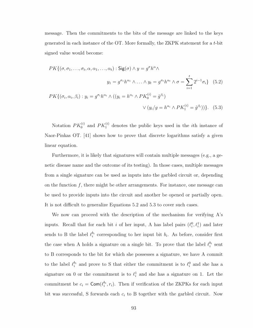
message. Then the commitments to the bits of the message are linked to the keys

generated in each instance of the OT. More formally, the ZKPK statement for a t-bit

signed value would become:

PK{(�, �1

, . . ., �t

,↵,↵1

, . . .,↵t

) : Sig(�) ^ y = g�h↵^

y1

= g�1h↵1 ^ . . . ^ yt

= g�th↵

t ^ � =tX

i=1

2i�1�i

} (5.2)

PK{(�i

,↵i

, �i

) : yi

= g�ih↵

i ^ ((yi

= h↵

i ^ PK(i)

0

= g�i)

_ (yi

/g = h↵

i ^ PK(i)

1

= g�i))}. (5.3)

Notation PK(i)

0

and PK(i)

1

denotes the public keys used in the ith instance of

Naor-Pinkas OT. [41] shows how to prove that discrete logarithms satisfy a given

linear equation.

Furthermore, it is likely that signatures will contain multiple messages (e.g., a ge-

netic disease name and the outcome of its testing). In those cases, multiple messages

from a single signature can be used as inputs into the garbled circuit or, depending

on the function f , there might be other arrangements. For instance, one message can

be used to provide inputs into the circuit and another be opened or partially open.

It is not di�cult to generalize Equations 5.2 and 5.3 to cover such cases.

We now can proceed with the description of the mechanism for verifying A’s

inputs. Recall that for each bit i of her input, A has label pairs (`0i

, `1i

) and later

sends to B the label `bii

corresponding to her input bit bi

. As before, consider first

the case when A holds a signature on a single bit. To prove that the label `bii

sent

to B corresponds to the bit for which she possesses a signature, we have A commit

to the label `bii

and prove to S that either the commitment is to `0i

and she has a

signature on 0 or the commitment is to `1i

and she has a signature on 1. Let the

commitment be ci

= Com(`bii

, ri

). Then if verification of the ZKPKs for each input

bit was successful, S forwards each ci

to B together with the garbled circuit. Now

93

when A sends her input label `bii

to B, she is also required to open the commitment

ci

by sending ri

to B. B will proceed with circuit evaluation only if ci

= gˆ

`

b

i

i hr

i for

each bit i of A’s input, where ˆbii

and ri

are the values B received from A.

More formally, the statement A proves to S in ZK is PK{(�,↵, �, �) : Sig(�)^y =

g�h↵ ^ z = g�h� ^ ((y = h↵ ^ z/g`0i = h�)_ (y/g = h↵ ^ z/g`1i = h�))}. Similar to the

case of B’s input verification, this ZKPK can be generalized to use a single signature

with multiple bits input into the circuit. More precisely, the statement in Equation

5.2 remains unchanged, while the second statement becomes:

PK{(�i

,↵i

, �i

, �i

) : yi

= g�ih↵

i ^ zi

= g�ih�

i^

((yi

= h↵

i ^ zi

/g`0i = h�

i) _ (yi

/g = h↵

i ^ zi

/g`1i = h�

i))}. (5.4)

We summarize the overall solution as Protocol 3 below.

The security of Protocol 3 can be stated as follows:


malicious A or B and semi-honest S in the hybrid model with ideal implementation

of OT and where H is a hash function modeled as a random oracle and inputs of A

and B are verified according to Definition 4.

Because the structure of the computation in Protocol 3 is the same as in Protocol

2 and primarily only ZKPKs have been added (that have corresponding simulators

in the ideal model), we do not mention the proof here.

5.6 Private Genomic Computation

For all types of genomic computation we assume that A has information extracted

from her genome, which she privately stores. Similarly, B stores data associated with

his genome. A and B may enter some or all of their data into the computation and

94


and signature Sig(x1

), B has private input x2

andSig(x

2

), and S has no private input.Output: A and B learn f(x

1

, x2


1. (a) S chooses �R! {0, 1}�1, k

1

R! {0, 1}, k2

R! {0, 1} and sets � = �||1.S sends � and k

1

to A. S also computes labels `0i

= PRF(k1

, i) and`1i

= `0i

�� for i 2 [1, t1

].

(b) A computes labels `0i

= PRF(k1

, i) and `1i

= `0i

� � for i 2 [1, t1

]. Foreach bit b

i

of her input, A commits ci

= Com(bi

, ri

) and c0i

= Com(`bii

, r0i

)using fresh randomness r

i

and r0i

. A sends to S Sig(x1

) and ci

, c0i

fori 2 [1, t

1

].

(c) A proves in ZK the statement in Equation 5.2 using private inputsx1

, b1

, . . ., bt1 , r1, . . ., rt1 . For each i 2 [1, t

1

], A also proves in ZK thestatement in Equation 5.4 using private inputs b

i

, ri

, `bii

, r0i

.

2. S computes wire labels `0i

= PRF(k2

, i� t1

) and `1i

= `0i

�� for i 2 [t1

+1,m].S then construct garbled gates G

f

and sends Gf

and A’s commitments c0i

fori 2 [1, t

1

] to B.

3. S and B engage in t2

instances of 1-out-of-2 OT as in Protocol 2 together withverification of B’s input. Before B can learn labels `bi

t1+i

, B forms t2

commit-ments c00

i

= Com(bi

, r00i

) using fresh randomness r00i

and proves in ZK the state-ments in Equations 5.2 and 5.3 using private input x

2

, b1

, . . ., bt2 , r

001

, . . ., r00t2

and bi

, r00i

, ki

, respectively. Here ki

denotes the value chosen during step 2 ofthe ith instance of the OT protocol.

4. A opens commitments c0i

by sending to B pairs (`bii

, r0i

) for i 2 [1, t1

]. B checkswhether Com(`

i

, r0i

) = c0i

for each i and aborts if at least one check fails.

5. The remaining steps are the same as in Protocol 2.

95

they may also compute a function of their individual data, which will be used as the

input into the joint computation.

5.6.1 Ancestry Test

This test would often be invoked when A and B already know to be related or

have reasons to believe to be related. Under such circumstances, they are unlikely

to try to cheat each other. For that reason, we use the solution with semi-honest A

and B to realize this test. Because SNP-based tests are most general and can provide

information about recent as well as distant ancestry, we build a circuit that takes a

large number of SNPs from two individuals and counts the number of positions with

the same values. The computed value is then compared to a number of thresholds to

determine the closest generation in which the individuals have the same ancestor.

To compute the number of SNPs which are equal in the DNA of two individuals,

the circuit first proceeds by XORing two binary input vectors from A and B (recall

that the value of each SNP is a bit) and then counts the number of bits that di↵er

in a hierarchical manner. That is, in the first round of additions, every two adjacent

bits are added and the result is a 2-bit integer. In the second round of additions,

every two adjacent results from the first round are added resulting in 3-bit sums.

This process continues in dlog2

te rounds of additions, where t is the size of A’s and

B’s input, and the last round performs only a single addition. As mentioned earlier,

the result can be interpreted by performing a number of comparisons at the end, but

the cost of final comparisons is insignificant compared to the remaining size of the

circuit.

5.6.2 Paternity Test

We assess that the security setting with malicious users A and B is the most suit-

able for running paternity tests. That is, the participants may be inclined to tamper

96

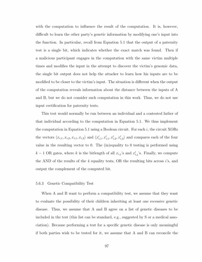
with the computation to influence the result of the computation. It is, however,

di�cult to learn the other party’s genetic information by modifying one’s input into

the function. In particular, recall from Equation 5.1 that the output of a paternity

test is a single bit, which indicates whether the exact match was found. Then if

a malicious participant engages in the computation with the same victim multiple

times and modifies the input in the attempt to discover the victim’s genomic data,

the single bit output does not help the attacker to learn how his inputs are to be

modified to be closer to the victim’s input. The situation is di↵erent when the output

of the computation reveals information about the distance between the inputs of A

and B, but we do not consider such computation in this work. Thus, we do not use

input certification for paternity tests.

This test would normally be run between an individual and a contested father of

that individual according to the computation in Equation 5.1. We thus implement

the computation in Equation 5.1 using a Boolean circuit. For each i, the circuit XORs

the vectors hxi,1

, xi,2

, xi,1

, xi,2

i and hx0i,1

, x0i,1

, x0i,2

, x0i,2

i and compares each of the four

value in the resulting vector to 0. The (in)equality to 0 testing is performed using

k � 1 OR gates, where k is the bitlength of all xi,j

’s and x0i,j

’s. Finally, we compute

the AND of the results of the 4 equality tests, OR the resulting bits across i’s, and

output the complement of the computed bit.

5.6.3 Genetic Compatibility Test

When A and B want to perform a compatibility test, we assume that they want

to evaluate the possibility of their children inheriting at least one recessive genetic

disease. Thus, we assume that A and B agree on a list of genetic diseases to be

included in the test (this list can be standard, e.g., suggested by S or a medical asso-

ciation). Because performing a test for a specific genetic disease is only meaningful

if both parties wish to be tested for it, we assume that A and B can reconcile the

97

di↵erences in their lists.

To maximize privacy, we construct the function f to be as conservative as possible.

In particular, given a list of genetic diseases L, A and B run a compatibility test for

each disease D 2 L, and if at least one test resulted in a positive outcome, the

function will output 1, and otherwise it will output 0. That is, the function can

be interpreted as producing 1 if A and B’s children have a chance of inheriting the

major variety for at least one of the tested diseases; and producing 0 means that their

children will not inherit the major variety for any of the diseases in L. Evaluating

this function can be viewed as the first step in A and B’s interaction. If the output

was 1, they may jointly decide to run more specific computation to determine the

responsible disease or diseases themselves.

The above means that for each D 2 L, A can locally run the test to determine

whether she is a carrier of D. B performs the same test on his data. Thus, A’s and

B’s input into f consists of |L| bits each and the result is 1 i↵ 9i such that A’s and

B’s ith input bits are both 1. This computation can be realized as a simple circuit

consisting of |L| AND and |L|� 1 OR gates.

Next, notice is that it is easy for malicious A or B to learn sensitive information

about the other party by using certain inputs. That is, if a malicious user sets all

his input bits to 1, he will be able to learn whether the other party is a carrier

of least one disease in L. This poses substantial privacy concerns, particularly for

matchmaking services that routinely run genetic compatibility tests between many

individuals. Thus, we require that A and B certify the results of testing for each

genetic disease on the list (e.g., by a medical facility) and enter certified inputs into

the computation. (Note that the medical facility that performs sequencing can also

certify the test results; alternatively, the medical facility performing test certification

will require genome certification from the facility that performed sequencing.) This

means that the server-aided solution with certified inputs will be used for secure

98

computation.

For each disease D 2 L, the signature will need to include the name of the disease

D and the test outcome �, which we assume is a bit. Then if we target e�cient the

computation, the disease names will not be input into the circuit, but instead S will

verify that A’s signature used for a particular input wire includes the same disease

name as B’s signature used for an equivalent input wire. A simple way to achieve this

is to reveal list L to S and reveal the name of the disease including in each signature

(without revealing the signature itself). If we assume that each issued signature is

on the tuple (D, �), i.e., the signature was produced as ve ⌘ aD1

a�2

bsc, all that is

needed is to adjust the value used in the ZKPK of the signature by 1

a

D

2by both the

sender and the verifier for each D 2 L (we refer the reader to [37] for details). S

will need to check that all conditions appear in the same order among A’s and B’s

inputs (i.e., the sequences of diseases are identical) before proceeding with the rest of

the protocol. Revealing the set of diseases used in the compatibility test would not

constitute violation of privacy if such a set of conditions is standard or suggested by

S itself.

When, however, the parties compose a custom set of genetic diseases for their

genetic compatibility testing and would like to keep the set private, they may be

unwilling reveal the set of diseases to S. We propose that the parties instead prove that

they are providing results for the same conditions without revealing the conditions

themselves to the server. The di�culty in doing so arises from the fact that S interacts

independently with A and B (possibly at non-overlapping times) and A and B are

not proving any joint statements together. Our idea of proving that inputs of A

and B correspond to the same sequence of diseases consists of forming a sequence

of commitments to the diseases in L, the openings of which are known to both

A and B. That is, A and B jointly generate a commitment to each disease using

shared randomness and used those commitments at the time of proving that their

99

inputs have been certified. Then if A supplies commitments Com1

, . . . , Comt

and

proves that the committed values correspond to the diseases in her signatures, S will

check that B supplies the same sequence of commitments and also proves that the

committed values are equal to the diseases in the signatures he possesses. This will

ensure that A and B supply input bits for the same sequence of diseases. To jointly

produce the commitments, we have both A and B contribute their own randomness

and the resulting commitment will be a function of A’s and B’s contribution. It can

proceed as follows (recall that A and B can be malicious):

1. A chooses a random rA

and sends to B cA

= Com(rA

, z).

2. B chooses a random rB and sends to A

3. A and B open their commitments by exchanging (rA

, z) and (rB

, z0) and verifythat they match c

A

and cB

, resp.

4. They form joint randomness as r = rA

�rB

and use it to construct commitmentCom(D, r).

Then the (high-level) statement that A and B prove about their inputs is PK{(↵, �) :

Sig(↵, �)^ y1

= Com(↵)^ y2

= Com(�)} using y1

shared between A and B, while the

remaining portion is specific to A and B as detailed in Section 5.5.3.

5.7 Performance Evaluation

In this section, we report on the results of our implementation. The implemen-

tation used Miracl library [47] for large number arithmetic and JustGarble library

[25] for garbled circuit implementation. We provide experimental results for ancestry,

paternity, and compatibility tests implemented as described in Section 5.6. The se-

curity parameters for symmetric key cryptography and statistical security were set to

128. The security parameter for public key cryptography (for both RSA modulus and

discrete logarithm setting) was set to 1536. Additionally, the security parameter for

the group size in the discrete logarithm setting was set to 192. Note that in practice

100

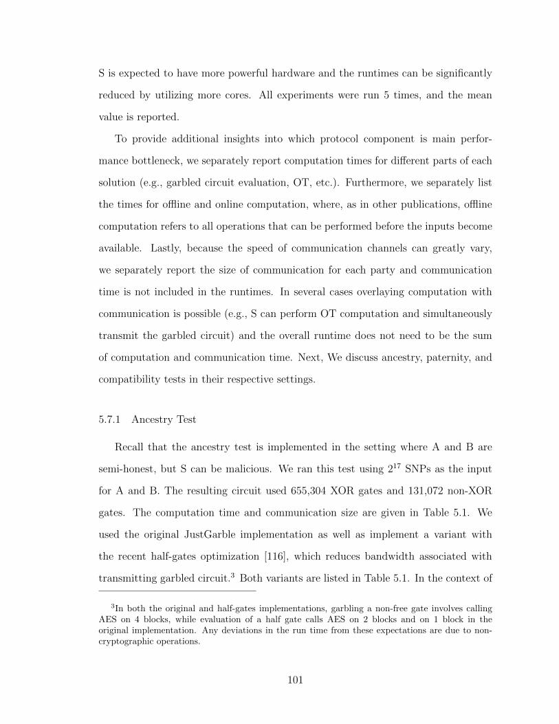
S is expected to have more powerful hardware and the runtimes can be significantly

reduced by utilizing more cores. All experiments were run 5 times, and the mean

value is reported.

To provide additional insights into which protocol component is main perfor-

mance bottleneck, we separately report computation times for di↵erent parts of each

solution (e.g., garbled circuit evaluation, OT, etc.). Furthermore, we separately list

the times for o✏ine and online computation, where, as in other publications, o✏ine

computation refers to all operations that can be performed before the inputs become

available. Lastly, because the speed of communication channels can greatly vary,

we separately report the size of communication for each party and communication

time is not included in the runtimes. In several cases overlaying computation with

communication is possible (e.g., S can perform OT computation and simultaneously

transmit the garbled circuit) and the overall runtime does not need to be the sum

of computation and communication time. Next, We discuss ancestry, paternity, and

compatibility tests in their respective settings.

5.7.1 Ancestry Test

Recall that the ancestry test is implemented in the setting where A and B are

semi-honest, but S can be malicious. We ran this test using 217 SNPs as the input

for A and B. The resulting circuit used 655,304 XOR gates and 131,072 non-XOR

gates. The computation time and communication size are given in Table 5.1. We

used the original JustGarble implementation as well as implement a variant with

the recent half-gates optimization [116], which reduces bandwidth associated with

transmitting garbled circuit.3 Both variants are listed in Table 5.1. In the context of

3In both the original and half-gates implementations, garbling a non-free gate involves calling

AES on 4 blocks, while evaluation of a half gate calls AES on 2 blocks and on 1 block in the

original implementation. Any deviations in the run time from these expectations are due to non-

cryptographic operations.

101

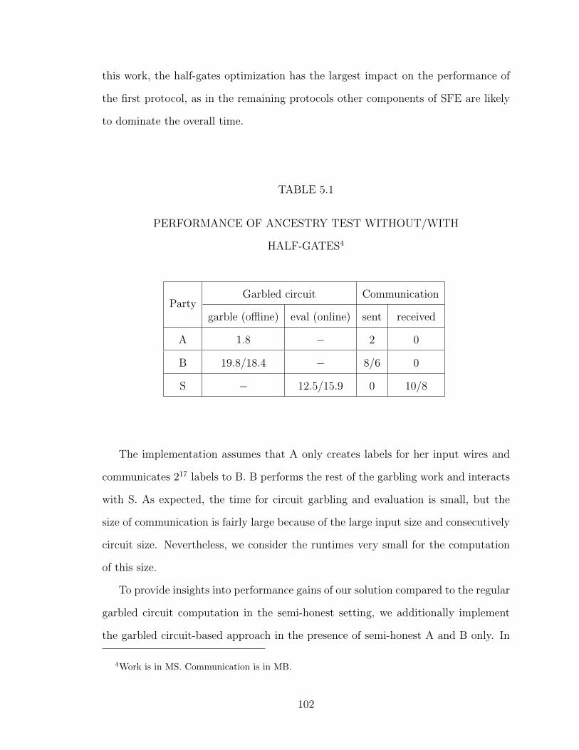
this work, the half-gates optimization has the largest impact on the performance of

the first protocol, as in the remaining protocols other components of SFE are likely

to dominate the overall time.

TABLE 5.1

PERFORMANCE OF ANCESTRY TEST WITHOUT/WITH

HALF-GATES4

PartyGarbled circuit Communication

garble (o✏ine) eval (online) sent received

A 1.8 � 2 0

B 19.8/18.4 � 8/6 0

S � 12.5/15.9 0 10/8

The implementation assumes that A only creates labels for her input wires and

communicates 217 labels to B. B performs the rest of the garbling work and interacts

with S. As expected, the time for circuit garbling and evaluation is small, but the

size of communication is fairly large because of the large input size and consecutively

circuit size. Nevertheless, we consider the runtimes very small for the computation

of this size.

To provide insights into performance gains of our solution compared to the regular

garbled circuit computation in the semi-honest setting, we additionally implement

the garbled circuit-based approach in the presence of semi-honest A and B only. In

4Work is in MS. Communication is in MB.

102

addition to circuit garbling and evaluation, this also requires the use of OT, which we

implement using a recent optimized OT extension construction from [14] (including

optimizations specific to Yao’s garbled circuit evaluation). As in [14], we use Naor-

Pinkas OT for 128 base OTs [99]. The results are given in Table 5.2. Compared to

the server-aided setting, computation is higher by at least two orders of magnitude

for each party and communication is noticeably increased as well.

TABLE 5.2

PERFORMANCE OF ANCESTRY TEST WITHOUT SERVER

WITHOUT/WITH HALF-GATES5

PartyGarbled circuit OT Total time Comm

garble eval o✏ineonline o✏ine online sent received

A 21.6/20.2 � 195.2 1983 216.8/215.4 1983 10.02/8.02 2.03

B � 12.5/15.9 2003 218.6 2003 231.1/234.5 2.03 10.02/8.02

5.7.2 Paternity Test

Next, we look at the paternity test, implemented as described in Section 5.6 in

the presence of malicious A and B and semi-honest S. The inputs for both A and

B consisted of 13 2-element sets, where each element is 9 bits long. We use OT

extension from [14] with 128 Naor-Pinkas base OTs. The circuit consisted of 468

5Work is in MS. Communication is in MB.

103

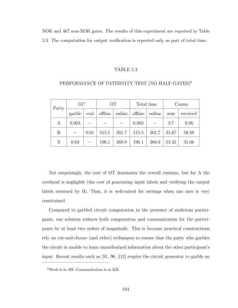
XOR and 467 non-XOR gates. The results of this experiment are reported in Table

5.3. The computation for output verification is reported only as part of total time.

TABLE 5.3

PERFORMANCE OF PATERNITY TEST (NO HALF-GATES)6

PartyGC OT Total time Comm

garble eval o✏ine online o✏ine online sent received

A 0.003 � � � 0.003 � 3.7 0.06

B � 0.01 515.5 201.7 515.5 201.7 31.67 56.88

S 0.03 � 196.1 260.9 196.1 260.9 53.32 31.66

Not surprisingly, the cost of OT dominates the overall runtime, but for A the

overhead is negligible (the cost of generating input labels and verifying the output

labels returned by B). Thus, it is well-suited for settings when one user is very

constrained.

Compared to garbled circuit computation in the presence of malicious partici-

pants, our solution reduces both computation and communication for the partici-

pants by at least two orders of magnitude. This is because practical constructions

rely on cut-and-choose (and other) techniques to ensure that the party who garbles

the circuit in unable to learn unauthorized information about the other participant’s

input. Recent results such as [91, 96, 112] require the circuit generator to garble on

6Work is in MS. Communication is in KB.

104

the order of 125 circuits for cheating probability of at most 2�40, some of which are

checked (i.e., re-generated) by the circuit evaluator, while the remaining circuits are

evaluated. Thus, the work of each of A and B will have to increase by at least two

orders of magnitude just for circuit garbling and evaluation, not counting other tech-

niques that deter a number of known attacks and result in increasing the input size

and introducing expensive public key operations. A notable exception to the above

is the work of Lindell [89] that reduces the number of circuits to 40 for the same

cheating probability. The construction, however, results in savings only for circuits

of large size as it introduces a large number of additional public key operations. Thus,

for paternity tests using constructions with a larger number of circuits is very likely

to be faster in practice, which results in a drastic di↵erence between our solution

and regular garbled circuit protocol with malicious participants. This di↵erence in

performance can be explained by the fact that in our setting one party is known not

to deviate from the protocol allowing for a more e�cient solution.

Baldi et al. [20] also provide a private paternity test in the two-party setting

(between a client and a server). It uses a di↵erent computation based on Restriction

Fragment Length Polymorphisms (RFLPs) and relies on private set intersection as

a cryptographic building block. Both o✏ine and online times for the client and the

server are 3.4 ms and the communication size is 3KB for the client and 3.5KB for the

server when the test is performed with 25 markers. All times and communication sizes

double when the test is run with 50 markers. While the runtimes we report are higher,

the implementation of [20] did not consider malicious participants. If protection

against malicious A and B in our solution is removed, the work for all parties reduces

to well below 0.1 millisecond and communication becomes a couple of KBs.

105

5.7.3 Genetic Compatibility Test

The last genetic compatibility test is run in the setting where A and B are mali-

cious and their inputs must be certified. We choose the variant of the solution that

reveals the list of diseases L to the server (i.e., a standard list is used). We imple-

ment the signature scheme, OT, and ZKPKs as described earlier. All ZKPKs are

non-interactive using the Fiat-Shamir heuristic [59]. We used |L| = 10 and thus A

and B provide 10 input bits into the circuit accompanied by 10 signatures. The circuit

consisted of only 19 non-XOR gates. The performance of the test is given in Table

5.4. We divide all ZKPKs into a proof of signature possession (together with a com-

mitment), denoted by “Sign PK” in the table, and the remaining ZK proofs, denoted

by “Other PK.” As it is clear from the table, input certification contributes most of

the solution’s overhead, but it is still on the order of 1–3 seconds for all parties.

TABLE 5.4

PERFORMANCE OF COMPATIBILITY TEST (NO HALF-GATES)7

PartyGarbled circuit OT Sign PK Other PK Total time Comm

garble

eval

o✏ine

online

o✏ine

online

o✏ine

online

o✏ine

online

sent

received

A 0 � � � 1170 42.1 616.8 20.6 1790 62.7 34.35 0.06

B � 0.001 15.4 14.6 1170 42.1 282.4 15.7 1470 72.4 36.41 2.98

S 0.003 � 29.3 15.2 0 2060 0 756 29.3 2830 2.87 70.59

7Work is in MS. Communication is in KB.

106

As mentioned earlier, we are not aware of general results that achieve input certi-

fication for comparison. However, the comparison to general garbled circuit compu-

tation in the presence of malicious parties or server-aided garbled circuit computation

from Section 5.7.2 applies here as well.

Baldi et al. [20] also build a solution and report on the performance of genetic

compatibility test. In [20], testing for presence of a genetic disease that client carries

in the server genome consists of the client providing the disease fingerprint in the

form of (nucleotide, location) pairs (which is equivalent to a SNP) and both parties

searching whether the disease fingerprint also appears in the server’s DNA. This

requires scanning over the entire genome, which our solution avoids. As a result,

the solution of [20] incurs substantial o✏ine overhead for the server (67 minutes)

and large communication size (around 4GB) even for semi-honest participants. The

solution utilizes authorized private set intersection, which allows inputs of one party

(as opposed to both in our work) to be verified. Compared to [20], in our framework,

testing for a single disease requires a fraction of a second for each party with malicious

A and B, where inputs of both of them are certified. The computation is greatly

simplified because the list of diseases is assumed to be known by both users. When

this is the case, the cost of input certification greatly dominates the overall time.

107

CHAPTER 6

FINGERPRINT RECOGNITIONS

Fingerprint is one of the most accurate type of biometric data that used for ver-

sification and identification; therefore, protecting the data is crucial during the fin-

gerprint recognition computations. In this chapter, we present three secure privacy-

preserving protocols for fingerprint alignment and matching, based on what are con-

sidered to be the most precise and e�cient fingerprint recognition algorithms—those

based on the geometric matching of “landmarks” known as minutia points. Our

protocols allow two or more honest-but-curious parties to compare their respective

privately-held fingerprints in a secure way such that they each learn nothing more

than a highly-accurate score of how well the fingerprints match. To the best of our

knowledge, this is the first time fingerprint alignment based on minutiae is considered

in a secure computation framework.

In this chapter, we briefly describe motivation and contributions in Sections 6.1

and 6.2. Section 6.3 provides necessary fingerprint background, including the three

fingerprint comparison algorithms which are the focus of this work. Section 6.4 de-

scribes the problem statement which we rely to realize secure fingerprint comparisons.

Then Section 6.5 describes new secure sub-protocols not available in the prior litera-

ture that we design to enable secure fingerprint comparisons. Our main protocols for

the three selected fingerprint alignment and matching algorithms are given in Sec-

tion 6.6. Lastly, experimental evaluation of our secure realization of the third spectral

minutia representation algorithm in two di↵erent secure computation frameworks is

given in Section 6.7.

108

6.1 Motivation

Computing securely with biometric data is challenging because biometric identi-

fication applications often require accurate metrics and recognition algorithms, but

the data involved is so sensitive that if it is ever revealed or stolen the victim may be

vulnerable to impersonation attacks for the rest of their life. This risk is particularly

true for fingerprints, which have been used since the 19th century for identifica-

tion purposes and are being used for such purposes ubiquitously today, including for

cellphones, laptops, digital storage devices, safes, immigration, and physical build-

ing/room access, as well as the classic application of identifying criminals. Thus,

there is a strong motivation for fast and secure fingerprint recognition protocols that

protect fingerprint data but nevertheless allow for highly accurate scores for finger-

print comparison.

6.2 Contributions

The setting we consider in this work is one where the parties involved are honest-

but-curious (although, in some cases, malicious parties can also be tolerated using

known hardening techniques). That is, two or more parties hold private fingerprint

data that they would like to compare in a fast way that provides an accurate score

for the comparison but does not reveal the actual fingerprint data. For example,

the computation could involve comparing multiple pairs of fingerprint representa-

tions stored in two privacy-sensitive databases (e.g., one owned by the FBI and the

other owned by a university), or it could involve a single comparison of a suspected

criminal’s fingerprint to a fingerprint found at a crime scene.

According to accepted best practices (e.g., see [92, 98, 115]) the most accurate

fingerprint recognition algorithms are based on the use of minutia points, which are

fingerprint “landmarks,” such as where two ridges merge or split. (See Figure 6.1.)

109

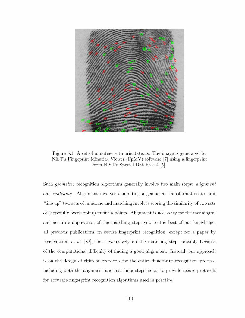
Figure 6.1. A set of minutiae with orientations. The image is generated byNIST’s Fingeprint Minutiae Viewer (FpMV) software [7] using a fingerprint

from NIST’s Special Database 4 [5].

Such geometric recognition algorithms generally involve two main steps: alignment

and matching. Alignment involves computing a geometric transformation to best

“line up” two sets of minutiae and matching involves scoring the similarity of two sets

of (hopefully overlapping) minutia points. Alignment is necessary for the meaningful

and accurate application of the matching step, yet, to the best of our knowledge,

all previous publications on secure fingerprint recognition, except for a paper by

Kerschbaum et al. [82], focus exclusively on the matching step, possibly because

of the computational di�culty of finding a good alignment. Instead, our approach

is on the design of e�cient protocols for the entire fingerprint recognition process,

including both the alignment and matching steps, so as to provide secure protocols

for accurate fingerprint recognition algorithms used in practice.

110

In this work, we focus on three algorithms that compare fingerprints using both

alignment and matching:

1. A simple geometric transformation algorithm that searches for the maximummatching by considering each pair of minutia [92].

2. An algorithm aligns fingerprints based on high curvature points [98].

3. An algorithm based on a spectral minutia representation [115].

These algorithms were selected due to their precision, speed, and/or popularity,

with the goal of building e�cient and practical security solutions. Our main contri-

butions can be summarized as follows:

• We design new secure sine, cosine, and arctangent sub-protocols for fixed-pointarithmetic, for both two-party (garbled circuit) and multi-party (secret sharing)cases.

• We design a new secure square-root sub-protocol for fixed-point arithmetic.Our solution is for the two-party (garbled circuit) setting and is based on Gold-schmidt’s method with the last iteration replaced by Newton-Raphson’s methodto eliminate accumulated errors.

• We design a new secure sub-protocol for selecting the fth smallest element ina set of comparable elements. Our method is based on an e�cient square-rootsampling algorithm.

• We build three secure and e�cient protocols for fingerprint alignment andmatching, based on the use of the above new building blocks applied to the threewell-known fingerprint recognition algorithms mentioned above. The construc-tions work in both two-party (garbled circuit) and multi-party (secret sharing)settings.

• We implement one of the secure fingerprint recognition protocols and show itse�ciency in practice.

Our constructions are presented in the semi-honest model. However, a number

of available techniques can be used to achieve security in the malicious model (e.g.,

[13, 54, 64] and others in the multi-party (secret sharing) setting and [87] among

others in the two-party (garbled circuit) setting).

111

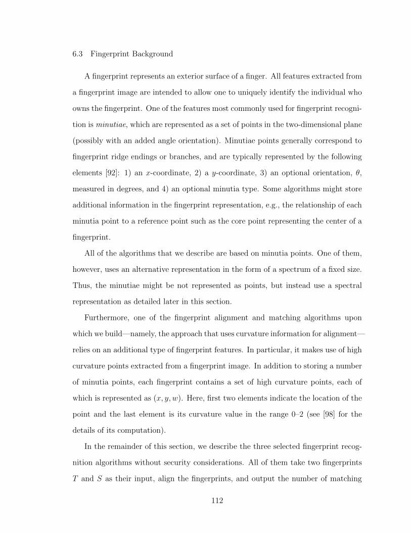
6.3 Fingerprint Background

A fingerprint represents an exterior surface of a finger. All features extracted from

a fingerprint image are intended to allow one to uniquely identify the individual who

owns the fingerprint. One of the features most commonly used for fingerprint recogni-

tion is minutiae, which are represented as a set of points in the two-dimensional plane

(possibly with an added angle orientation). Minutiae points generally correspond to

fingerprint ridge endings or branches, and are typically represented by the following

elements [92]: 1) an x-coordinate, 2) a y-coordinate, 3) an optional orientation, ✓,

measured in degrees, and 4) an optional minutia type. Some algorithms might store

additional information in the fingerprint representation, e.g., the relationship of each

minutia point to a reference point such as the core point representing the center of a

fingerprint.

All of the algorithms that we describe are based on minutia points. One of them,

however, uses an alternative representation in the form of a spectrum of a fixed size.

Thus, the minutiae might be not represented as points, but instead use a spectral

representation as detailed later in this section.

Furthermore, one of the fingerprint alignment and matching algorithms upon

which we build—namely, the approach that uses curvature information for alignment—

relies on an additional type of fingerprint features. In particular, it makes use of high

curvature points extracted from a fingerprint image. In addition to storing a number

of minutia points, each fingerprint contains a set of high curvature points, each of

which is represented as (x, y, w). Here, first two elements indicate the location of the

point and the last element is its curvature value in the range 0–2 (see [98] for the

details of its computation).

In the remainder of this section, we describe the three selected fingerprint recog-

nition algorithms without security considerations. All of them take two fingerprints

T and S as their input, align the fingerprints, and output the number of matching

112

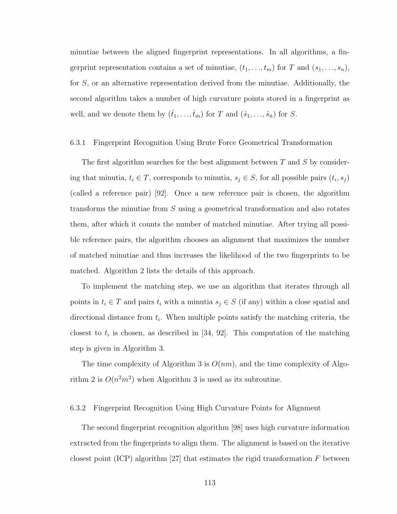
minutiae between the aligned fingerprint representations. In all algorithms, a fin-

gerprint representation contains a set of minutiae, (t1

, . . ., tm

) for T and (s1

, . . ., sn

),

for S, or an alternative representation derived from the minutiae. Additionally, the

second algorithm takes a number of high curvature points stored in a fingerprint as

well, and we denote them by (t1

, . . ., tm

) for T and (s1

, . . ., sn

) for S.

6.3.1 Fingerprint Recognition Using Brute Force Geometrical Transformation

The first algorithm searches for the best alignment between T and S by consider-

ing that minutia, ti

2 T , corresponds to minutia, sj

2 S, for all possible pairs (ti

, sj

)

(called a reference pair) [92]. Once a new reference pair is chosen, the algorithm

transforms the minutiae from S using a geometrical transformation and also rotates

them, after which it counts the number of matched minutiae. After trying all possi-

ble reference pairs, the algorithm chooses an alignment that maximizes the number

of matched minutiae and thus increases the likelihood of the two fingerprints to be

matched. Algorithm 2 lists the details of this approach.

To implement the matching step, we use an algorithm that iterates through all

points in ti

2 T and pairs ti

with a minutia sj

2 S (if any) within a close spatial and

directional distance from ti

. When multiple points satisfy the matching criteria, the

closest to ti

is chosen, as described in [34, 92]. This computation of the matching

step is given in Algorithm 3.

The time complexity of Algorithm 3 is O(nm), and the time complexity of Algo-

rithm 2 is O(n2m2) when Algorithm 3 is used as its subroutine.

6.3.2 Fingerprint Recognition Using High Curvature Points for Alignment

The second fingerprint recognition algorithm [98] uses high curvature information

extracted from the fingerprints to align them. The alignment is based on the iterative

closest point (ICP) algorithm [27] that estimates the rigid transformation F between

113

Algorithm 2: Fingerprint Recognition based on Geometrical Transformation

Input: Two fingerprints T = {ti

= (xi

, yi

, ✓i

)}mi=1

and S = {si

= (x0i

, y0i

, ✓0i

)}ni=1

.Output: The largest number of matching minutiae, C

max

, and thecorresponding alignment.

1. Initialize Cmax

= 0.

2. For i = 1, . . .,m and j = 1, . . ., n, use (ti

, sj

) as a reference pair and perform

(a) Compute transformation �x = x0j

� xi

, �y = y0j

� yi

, and �✓ = ✓0j

� ✓i

.

(b) Transfer each minutia sk

2 S as x00k

= cos(�✓) · x0k

+ sin(�✓) · y0k

��x,y00k

= � sin(�✓) · x0k

+ cos(�✓) · y0k

��y, and ✓00k

= ✓0k

��✓ and save theresult as S 00 = {s00

i

= (x00i

, y00i

, ✓00i

)}ni=1

.

(c) Compute the number C of matched minutiae between T and S 00 (e.g.,using Algorithm 3).

(d) If Cmax

< C, then set Cmax

= C and(�x

max

,�ymax

,�✓max

) = (�x,�y,�✓).

3. Return Cmax

and its corresponding alignment (�xmax

,�ymax

,�✓max

).

T and S. Once this transformation is determined, it is applied to the minutia points

of S. Then the algorithm computes the number of matched minutiae between T and

transformed S. The ICP algorithm assumes that the fingerprints are roughly pre-

aligned, which can be done, e.g., by aligning each fingerprint independently using

its core point, and iteratively finds point correspondences and the transformation

between them. To eliminate alignment errors when the overlap between the two sets

is partial, [98] suggests using the trimmed ICP (TICP) algorithm [48]. The TICP

algorithm ignores a proportion of the points in T whose distances to the corresponding

points in S are large, which makes it robust to outliers in the data.

The details of this fingerprint recognition approach are given in Algorithm 4.

Steps 1–10 correspond to the TICP algorithm that proceeds with iterations, aligning

the fingerprints closer to each in each successive iteration. The algorithm termination

parameters � and � correspond to the threshold for the total distance between the

matched points of T and S and the limit on the number of iterations, respectively.

114

Algorithm 3: Fingerprint matching

Input: Two fingerprints T = {ti

= (xi

, yi

, ✓i

)}mi=1

, S = {si

= (x0i

, y0i

, ✓0i

)}ni=1

andthresholds � and �

✓

for distance and orientation.Output: The number C of matched minutia pairs between T and S.

1. Set C = 0.

2. Mark each sj

2 S as available.

3. For i = 1, . . .,m, do

(a) Create a list Li

consisting of all available points sj

2 S that satisfy

min(|✓i

� ✓0j

|, 360� |✓i

� ✓0j

|) < �✓

andq

(xi

� x0j

)2 + (yi

� y0j

)2 < �.

(b) If Li

is not empty, select the closest minutia sk

to ti

from Li

, mark sk

asunavailable and set C = C + 1.

4. return C.

For robustness, the alignment is performed using only a subset of the points (f

closest pairs computed in step 4). The optimal motion for transforming one set of

the points into the other (treated as two 3-D shapes) is computed using the union

quaternion method due to Horn [73], and is given in Algorithm 5. The transformation

is represented as a 3 ⇥ 3 matrix R and a vector v of size 3, which are consequently

used to align the points in S (step 8).

Once the fingerprints are su�ciently aligned using the high curvature points, the

overall transformation between the original and aligned S is computed (step 11).

The resulting transformation is applied to the minutia points of S. The new x and y

coordinates of the minutiae can be computed directly using the transformation (R, v),

while orientation ✓ requires a special handling (since it is not used in computing the

optimal motion). We compute the di↵erence in the orientation between the original

and aligned S as the angle between the slopes of two lines drawn using two points

from the original and transformed S, respectively (step 12).

The original ICP algorithm [27] lists expected and worst case complexities of

computing the closest points (step 3 of Algorithm 4) to be O(m log n) and O(mn),

115

Algorithm 4: Fingerprint recognition based on high curvature points for align-mentInput: Two fingerprints consisting of minutiae and high curvature pointsT = ({t

i

= (xi

, yi

, ✓i

)}mi=1

, {ti

= (xi

, yi

, wi

)}mi=1

) and S = ({si

= (x0i

, y0i

, ✓0i

)}ni=1

,{s

i

= (x0i

, y0i

, w0i

)}ni=1

); a minimum number of matched high curvature pointsf ; and algorithm termination parameters � and �.Output: The largest number of matching minutiae, C, and the correspondingalignment.

1. Set SLTS

= 0.

2. Store a copy of si

’s as si

= (xi

, yi

, wi

) for i = 1, . . . , n.

3. For i = 1, . . ., n, find the closest to si

point tj

in T and store their distance di

.Here, the distance between any s

i

and tj

is defined asp(x0

i

� xj

)2 + (y0i

� yj

)2 + �|w0i

� wj

|.

4. Find f smallest di

’s and calculate their sum S 0LTS

.

5. If S 0LTS

� or � = 0, proceed with step 11.

6. Set SLTS

= S 0LTS

.

7. Compute the optimal motion (R, v) for the selected f pairs using Algorithm 5.

8. For i = 1, . . . , n, transform point si

according to (R, v) as si

= Rsi

+ v.

9. Set � = � � 1.

10. Repeat from step 3.

11. Compute the optimal motion (R, v) for n pairs (si

, si

) using Algorithm 5. Letri,j

denote R’s cell at row i and column j and vi

denote the ith element of v.

12. Compute c1

= (y2

� y1

)/(x2

� x1

), c2

= (y02

� y01

)(x02

� x01

), and�✓ = arctan((c

1

� c2

)/(1 + c1

c2

)).

13. For i = 1, . . ., n, apply the transformation to minutia si

by computingx0i

= r1,1

x0i

+ r1,2

y0i

+ v1

,y0i

= r2,1

x0i

+ r2,2

y0i

+ v2

,and ✓0

i

= ✓0i

��✓.

14. Compute the number, C, of matched minutiae between ti

’s and transformedsi

’s (e.g., using Algorithm 3).

15. Return C and the transformation (R, v).

116

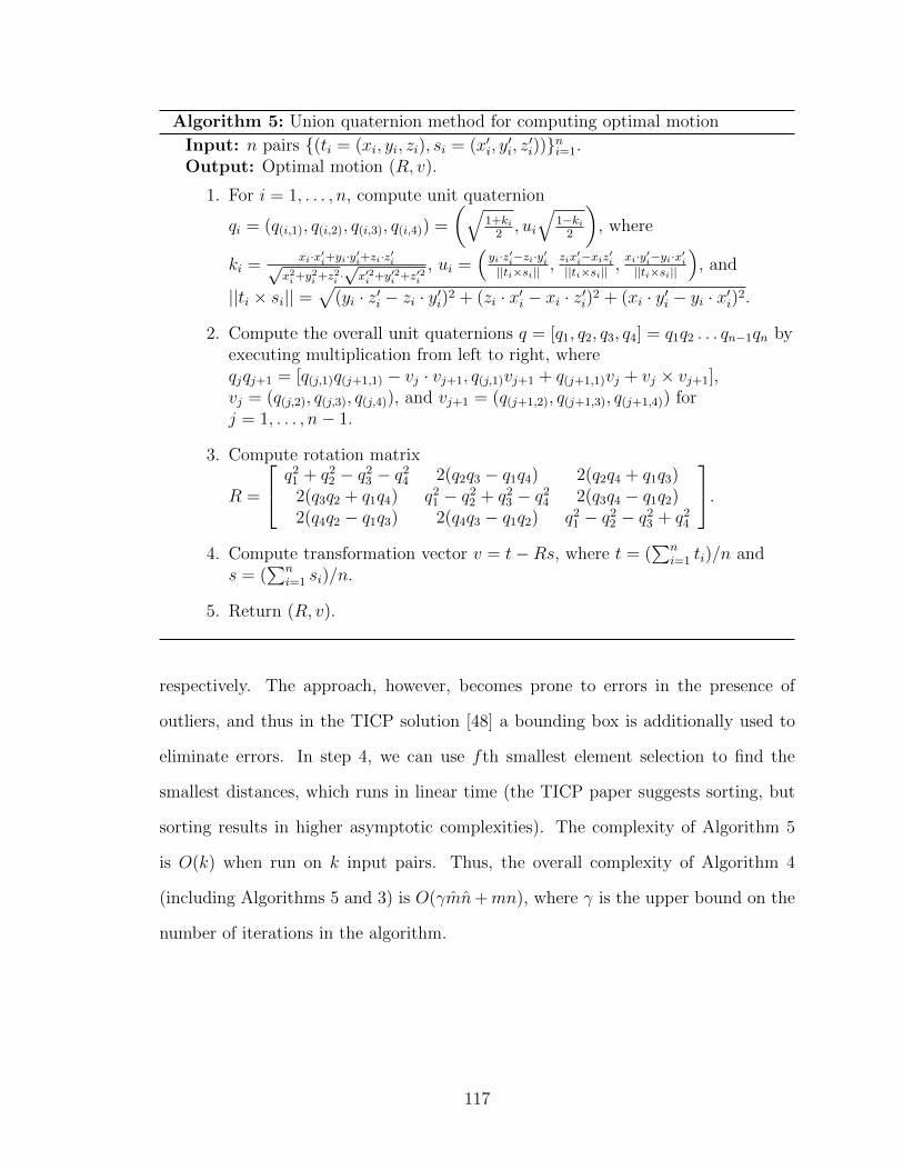
Algorithm 5: Union quaternion method for computing optimal motion

Input: n pairs {(ti

= (xi

, yi

, zi

), si

= (x0i

, y0i

, z0i

))}ni=1

.Output: Optimal motion (R, v).

1. For i = 1, . . . , n, compute unit quaternion

qi

= (q(i,1)

, q(i,2)

, q(i,3)

, q(i,4)

) =

✓q1+k

i

2

, ui

q1�k

i

2

◆, where

ki

= x

i

·x0i

+y

i

·y0i

+z

i

·z0ip

x

2i

+y

2i

+z

2i

·p

x

02i

+y

02i

+z

02i

, ui

=⇣

y

i

·z0i

�z

i

·y0i

||ti

⇥s

i

|| , zix0i

�x

i

z

0i

||ti

⇥s

i

|| ,x

i

·y0i

�y

i

·x0i

||ti

⇥s

i

||

⌘, and

||ti

⇥ si

|| =p(y

i

· z0i

� zi

· y0i

)2 + (zi

· x0i

� xi

· z0i

)2 + (xi

· y0i

� yi

· x0i

)2.

2. Compute the overall unit quaternions q = [q1

, q2

, q3

, q4

] = q1

q2

. . . qn�1

qn

byexecuting multiplication from left to right, whereqj

qj+1

= [q(j,1)

q(j+1,1)

� vj

· vj+1

, q(j,1)

vj+1

+ q(j+1,1)

vj

+ vj

⇥ vj+1

],vj

= (q(j,2)

, q(j,3)

, q(j,4)

), and vj+1

= (q(j+1,2)

, q(j+1,3)

, q(j+1,4)

) forj = 1, . . . , n� 1.

3. Compute rotation matrix

R =

2

4q21

+ q22

� q23

� q24

2(q2

q3

� q1

q4

) 2(q2

q4

+ q1

q3

)2(q

3

q2

+ q1

q4

) q21

� q22

+ q23

� q24

2(q3

q4

� q1

q2

)2(q

4

q2

� q1

q3

) 2(q4

q3

� q1

q2

) q21

� q22

� q23

+ q24

3

5.

4. Compute transformation vector v = t�Rs, where t = (P

n

i=1

ti

)/n ands = (

Pn

i=1

si

)/n.

5. Return (R, v).

respectively. The approach, however, becomes prone to errors in the presence of

outliers, and thus in the TICP solution [48] a bounding box is additionally used to

eliminate errors. In step 4, we can use fth smallest element selection to find the

smallest distances, which runs in linear time (the TICP paper suggests sorting, but

sorting results in higher asymptotic complexities). The complexity of Algorithm 5

is O(k) when run on k input pairs. Thus, the overall complexity of Algorithm 4

(including Algorithms 5 and 3) is O(�mn+mn), where � is the upper bound on the

number of iterations in the algorithm.

117

6.3.3 Fingerprint Recognition based on Spectral Minutiae Representation

The last fingerprint recognition algorithm by Xu et al. [115] uses minutia-based

representation of fingerprints, but o↵ers greater e�ciency than other algorithms be-

cause of an alternative form of minutia representation. The spectral minutia represen-

tation [114] that it uses is a fixed-length feature vector, in which rotation and scaling

can be easily compensated for, resulting in e�cient alignment of two fingerprints.

In the original spectral minutia representation [114], a set of minutiae corresponds

to a real-valued vector of a fixed length D, which is written in the form of a matrix

of dimensions M ⇥N (= D). The vector is normalized to have zero mean and unit

energy. Thus, we now represent T and S as matrices of dimensions M⇥N and denote

their individual elements as ti,j

’s and si,j

’s, respectively. In [114], there are two types

of minutia spectra (location-based and orientation-based), each with M = 128 and

N = 256, and a fingerprint represented by their combination consists of 65,536 real

numbers.

To compare two fingerprints in the spectral representation, two-dimensional cor-

relation is used as a measure of their similarity. Furthermore, to compensate for

fingerprint image rotations, which in this representation become circular shifts in the

horizontal direction, the algorithm tries a number of rotations in both directions and

computes the highest score among all shifts. This alignment and matching algorithm

is presented as Algorithm 6. It is optimized to perform shifts from �15 to 15 units

(which correspond to rotations from �10� to +10�) and computes only 9 similarity

scores instead of all 31 of them. Later in this section, we show how the algorithm can

be generalized to work with any amount of shift � resulting in only O(log �) score

computations.

Xu et al. [115] apply feature reduction to the spectral minutia representation to

reduce the size of the feature vector and consequently improve the time of fingerprint

comparisons without losing precision. That work describes two types of feature re-

118

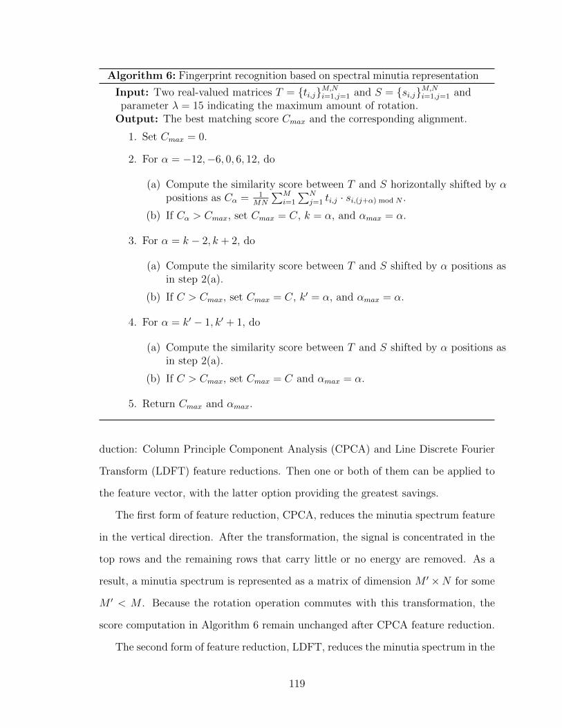
Algorithm 6: Fingerprint recognition based on spectral minutia representation

Input: Two real-valued matrices T = {ti,j

}M,N

i=1,j=1

and S = {si,j

}M,N

i=1,j=1

andparameter � = 15 indicating the maximum amount of rotation.Output: The best matching score C

max

and the corresponding alignment.

1. Set Cmax

= 0.

2. For ↵ = �12,�6, 0, 6, 12, do

(a) Compute the similarity score between T and S horizontally shifted by ↵positions as C

↵

= 1

MN

PM

i=1

PN

j=1

ti,j

· si,(j+↵) mod N

.

(b) If C↵

> Cmax

, set Cmax

= C, k = ↵, and ↵max

= ↵.

3. For ↵ = k � 2, k + 2, do

(a) Compute the similarity score between T and S shifted by ↵ positions asin step 2(a).

(b) If C > Cmax

, set Cmax

= C, k0 = ↵, and ↵max

= ↵.

4. For ↵ = k0 � 1, k0 + 1, do

(a) Compute the similarity score between T and S shifted by ↵ positions asin step 2(a).

(b) If C > Cmax

, set Cmax

= C and ↵max

= ↵.

5. Return Cmax

and ↵max

.

duction: Column Principle Component Analysis (CPCA) and Line Discrete Fourier

Transform (LDFT) feature reductions. Then one or both of them can be applied to

the feature vector, with the latter option providing the greatest savings.

The first form of feature reduction, CPCA, reduces the minutia spectrum feature

in the vertical direction. After the transformation, the signal is concentrated in the

top rows and the remaining rows that carry little or no energy are removed. As a

result, a minutia spectrum is represented as a matrix of dimension M 0 ⇥N for some

M 0 < M . Because the rotation operation commutes with this transformation, the

score computation in Algorithm 6 remain unchanged after CPCA feature reduction.

The second form of feature reduction, LDFT, reduces the minutia spectrum in the

119

horizontal direction and returns a feature matrix of dimension M ⇥N 0 (or M 0 ⇥N 0

if applied after the CPCA feature reduction) for some N 0 < N . The matrix consists

of complex numbers as a result of applying Fourier transform. After the LDFT, the

energy is concentrated in the middle columns and other columns are consequently

removed. Shifting matrix S in the resulting representation by ↵ positions now trans-

lates into setting its cell at location k, j to e�i

2⇡N

j↵·sk,j

, where i indicates the imaginary

part of a complex number. Note that circular shifts are no longer applied to matrix

rows (including when the LDFT is applied after the CPCA feature reduction).

The resulting matrices of complex numbers T and S are then converted to real-

valued matrices and processed using Algorithm 6. If we express a cell of T or S at

location k, j as ak,j

+ ibk,j

by separating its real and imaginary parts, then the kth

row of T and S is now expressed as a real-valued vector

r1

Nak,1

,

r2

Nak,2

, . . . ,

r2

Nak,N

,

r2

Nbk,2

, . . . ,

r2

Nbk,N

0 .

Computing the score between T and S then corresponds to computing the dot

product of each kth row of T and S and adding the values across all k. When

we use Algorithm 6 to compute the best similarity score, we need to adjust the

computation in step 2(a) for the new matrix dimensions and also implement rotation

as a multiplication instead of a shift. If we expand the quantity e�i

2⇡N

j↵ using the

formula ei' = cos(') + i sin('), the real part of each score between T and S rotated

by ↵ positions now becomes:

C↵

=1

MN2

M

0X

k=1

✓ak,1

✓a0k,1

cos

✓�2⇡↵

N

◆� b0

k,1

sin

✓�2⇡↵

N

◆◆+ (6.1)

+ 2N

0X

j=2

✓cos

✓�2⇡j↵

N

◆�ak,j

a0k,j

+ bk,j

b0k,j

�+ sin

✓�2⇡j↵

N

◆�a0k,j

bk,j

� ak,j

b0k,j

�◆!

where tk,j

= ak,j

+ ibk,j

and original sk,j

= a0k,j

+ ib0k,j

.

120

Returning to Algorithm 6, we generalize the algorithm to work for any value of

� so that only O(log �) score computations are necessary. Let � = c · 3k for some

constants c � 2 and k � 1. Our algorithm proceeds in k + 1 iterations computing c

scores in the first iteration and 2 scores in each consecutive iteration, which results in

the total of c+2k score computations. In the initial iteration 0, we compute c scores at

indices � = d3k/2e, . . ., d3k(2c� 1)/2e, then determine their maximum Cmax

and the

index of the maximum score ↵max

. In iteration i = 1, . . ., k, the algorithm computes

two scores at indices ↵max

± 3k�i, determines the maximum of the computed scores

and Cmax

, and updates the value of ↵max

as needed. Compared to Algorithm 6, this

approach covers 54 shifts using 8 score computations instead of 9 score computations

for 31 shifts. The best performance is achieved when � = 2 ·3k for some k. If � is not

of that form, we could use a di↵erent value of c, cover a wider range of shifts than

required, or decrease the step size of the algorithm slower than by a factor of 3 (as

was done in Algorithm 6), which results in redundant coverage.

In, [115], parameters M 0 and N 0 are chosen to retain most of the signal’s energy

after the transformations (e.g., 90%) and may be dependent on the data set. The

complexity of Algorithm 6 for two fingerprints after both types of feature reduction

is O(M 0N 0 log �).

6.4 Problem Statement

Because of the variety of settings in which fingerprint recognition may be used,

we distinguish between di↵erent computation setups and the corresponding security

settings.

1. There will be circumstances when two entities would like to compare fingerprintsthat they respectively possess without revealing any information about theirdata to each other. This can correspond to the cases when both entities own afingerprint database and would like to find entries common to both of them orwhen one entity would like to search a database belonging to a di↵erent entityfor a specific fingerprint. In these settings, the computation takes the form of

121

secure two-party computation, where the participants can be regarded as semi-honest or fully malicious depending on the application and their trust level.

2. There will also be circumstances when one or more data owners are computa-tionally limited and would like to securely o✏oad their work to more powerfulservers or cloud providers (this applies even if all fingerprints used in the com-putation belong to a single entity). Then multi-party settings that allow forinput providers to be di↵erent from the computational parties apply. In suchsettings, the computational parties are typically treated as semi-honest, butstronger security models can also be used for added security guarantees.

The focus of this work is on the semi-honest adversarial model, although standard

techniques for strengthening security in the presence of fully malicious participants

can be used as well.

In addition, to realize our constructions in a variety of settings, two secure com-

putation frameworks are of interest to us. In the two-party setting, we build on

garbled circuit evaluation techniques, while in the multi-party setting, we employ

linear secret sharing techniques.

6.5 Secure Building Blocks

To be able to build secure protocols for di↵erent fingerprint recognition algo-

rithms, we will need to rely on secure algorithms for performing a number of arith-

metic operations. Most of the computation described in Section 6.3 is performed on

real numbers, while for some of its components integer arithmetic will su�ce (e.g.,

Algorithm 3 can be executed on integers when its inputs are integer values). Com-

plex numbers are represented as a pair (a real part and an imaginary part) of an

appropriate data type.

For the purposes of this work, we choose to use fixed-point representation for real

numbers. Operations on fixed-point numbers are generally faster than operations

using floating-point representation (see, e.g., [11]), and fixed-point representation

provides su�cient precision for this application.

122

In Section 3.2.1, we listed building blocks from prior literature that we utilize

in our solutions. Now, we proceed with presenting our design for a number of new

building blocks for which we did not find secure realizations in the literature (Sec-

tion 6.5.1).

6.5.1 New Building Blocks

To build secure fingerprint recognition algorithms, we also need a number of se-

cure building blocks for rather complex operations that previously have not been

su�ciently treated in the literature. Thus, in this section, we present secure con-

structions for a number of operations, including trigonometric operations, square

root, and selection of the fth smallest element of a set.

We explore the available algorithms for computing these functions (e.g., Cheby-

shev polynomials for trigonometric functions) and build protocols that optimize per-

formance in each of the chosen settings of garbled circuit and secret sharing com-

putation. Our optimizations for designing the building blocks as well as the overall

protocols focus on the specific costs of the underlying techniques for secure arithmetic

and ensure that we achieve e�ciency together with precision and provable security

guarantees.

6.5.1.1 Sine, Cosine, and Arctangent

We now give new secure building blocks for three trigonometric functions, which

are sine, cosine, and arctangent. We denote secure protocols as [b] Sin([a]), [b]

Cos([a]), and [b] Arctan([a]) for each respective function. The output b is a fixed-

point value, while the input a (for sine and cosine) represented in degrees can be either

integer or fixed-point. For generality, we will assume that a used with trigonometric

functions is also a fixed-point value, while slight optimizations are possible when a is

known to be an integer (as in the fingerprint algorithms considered in this work).

123

There are a variety of di↵erent approximation algorithms that can be used for

trigonometric functions, many of which take the form of polynomial evaluation. Upon

examining the options, we chose to proceed with the polynomials described in [68,

Chapter 6], as they achieve good precision using only small degree polynomials. Note,

that Taylor series of trigonometric functions achieve an approximation when the

input is very close to a fixed point. However, in secure computation, we can only

assume the input value belongs to a known range (e.g., [0, 2⇡]). Therefore, polynomial

approximation over a range for inputs from [68] was chosen. The polynomials used in

[68] for trigonometric functions take the form P (x2) or xP (x2) for some polynomial

P over variable x (i.e., use only odd or even powers), which requires one to compute

only half as many multiplications as in a polynomial with all powers present.

The approach used in [68] o↵ers two types of polynomial approximations. The first

type uses a regular polynomial P (x) of degree N to approximate the desired function.

The second type uses a rational function of the form P (x)/Q(x), where P and Q are

polynomials of degree N and M , respectively. For the same desired precision, the

second option will yield lower degrees N and M and thus fewer multiplications to

approximate the function. This option, however, is undesirable when the division

operation is much costlier than the multiplication operation. In our setting, the

rational form is preferred in the case of garbled circuit evaluation (at least for higher

precisions) where multiplication and division have similar costs. However, with secret

sharing, the cost of division is much higher than that of multiplication, and we use

the first option with regular polynomial evaluation.

It is assumed in [68] that the initial range reduction to [0, ⇡/2] is used for the

input to trigonometric functions. This means that if input a to sine or cosine is

given in degrees, it needs to be reduced to the range [0, 90] and normalized to the

algorithm’s expectations. Note that it is straightforward to extend the result of the

computation to cover the entire range [0, 2⇡] given the output of this function and

124

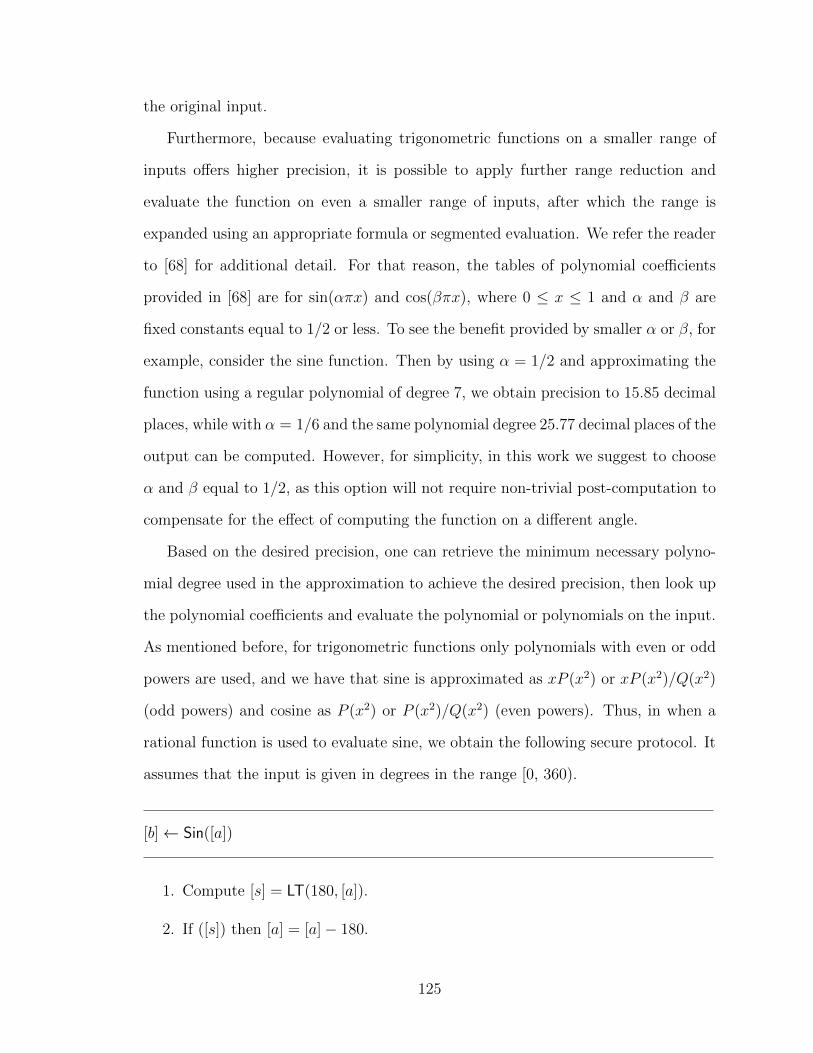
the original input.

Furthermore, because evaluating trigonometric functions on a smaller range of

inputs o↵ers higher precision, it is possible to apply further range reduction and

evaluate the function on even a smaller range of inputs, after which the range is

expanded using an appropriate formula or segmented evaluation. We refer the reader

to [68] for additional detail. For that reason, the tables of polynomial coe�cients

provided in [68] are for sin(↵⇡x) and cos(�⇡x), where 0 x 1 and ↵ and � are

fixed constants equal to 1/2 or less. To see the benefit provided by smaller ↵ or �, for

example, consider the sine function. Then by using ↵ = 1/2 and approximating the

function using a regular polynomial of degree 7, we obtain precision to 15.85 decimal

places, while with ↵ = 1/6 and the same polynomial degree 25.77 decimal places of the

output can be computed. However, for simplicity, in this work we suggest to choose

↵ and � equal to 1/2, as this option will not require non-trivial post-computation to

compensate for the e↵ect of computing the function on a di↵erent angle.

Based on the desired precision, one can retrieve the minimum necessary polyno-

mial degree used in the approximation to achieve the desired precision, then look up

the polynomial coe�cients and evaluate the polynomial or polynomials on the input.

As mentioned before, for trigonometric functions only polynomials with even or odd

powers are used, and we have that sine is approximated as xP (x2) or xP (x2)/Q(x2)

(odd powers) and cosine as P (x2) or P (x2)/Q(x2) (even powers). Thus, in when a

rational function is used to evaluate sine, we obtain the following secure protocol. It

assumes that the input is given in degrees in the range [0, 360).

[b] Sin([a])

1. Compute [s] = LT(180, [a]).

2. If ([s]) then [a] = [a]� 180.

125

3. If (LT(90, [a])) then [a] = 180� [a].

4. Compute [x] = 1

90

[a] and then [w] = [x]2.

5. Lookup the minimum polynomial degrees N and M using ↵ = 1/2 for whichprecision of the approximation is at least k bits.

6. Lookup polynomial coe�cients p0

, . . ., pN

and q0

, . . ., qM

for sine approximation.

7. Compute ([z1

], . . . , [zmax(N,M)

]) PreMul([w],max(N,M)).

8. Set [yP

] = p0

+P

N

i=1

pi

[zi

].

9. Set [yQ

] = q0

+P

M

i=1

qi

[zi

].

10. Compute [y] Div([yP

], [yQ

]).

11. If ([s]) then [b] = 0� [x] else [b] = [x].

12. Compute and return [b] = [b] · [y].

Recall that we recommend using a rational function in the form of P (x)/Q(x)

as in the above protocol for garbled circuit based implementation of high precision.

With secret sharing, we modify the protocol to evaluate only a single polynomial P

of (a di↵erent) degree N and skip the division operation in step 10. Also, based on

our calculations, the single polynomial variant is also slightly faster in the garbled

circuit setting when precision is not high (e.g., with 16 bits of precision).

As far as optimizations go, we, as usual, simultaneously execute independent

operations in the secret sharing setting. Also, note that because coe�cients pi

’s and

qj

’s are not integers, evaluations of polynomials in steps 8 and 9 is not local in the

secret sharing setting and requires truncation. We, however, can reduce the cost of

truncating N (respectively, M) values to the cost of one truncation. This is because

we first add the products and truncate the sum once. This also applies to polynomial

evaluation in other protocols such as cosine and arctangent.

When input a is known to lie in the range [0, 90] (as in the fingerprint algorithms

126

we consider in this work), steps 1, 2, 3, 11, and 12 are not executed and instead

we return [y] · [x] after evaluating step 10. Lastly, when input a is known to be an

integer, the comparisons in steps 1 and 3 and the multiplication of [a] and a fixed-

point constant 1

90

in step 4 become more e�cient in both secret sharing and garbled

circuit based implementations (i.e., both settings benefit from the reduced bitlength

of a if only integer part is stored and the cost of the multiplication in the secret

sharing setting becomes 1 interactive operation).

To show security of this protocol, we need to build simulators according to Defi-

nition 1. The main argument here is that because we only use secure building blocks

that do not reveal any private information, we apply Canetti’s composition theo-

rem [44] to result in security of the overall construction. More precisely, to simulate

the adversarial view, we invoke simulators corresponding to the building blocks. In

more detail, if we assume an implementation based on a (np, t)-threshold linear secret

sharing, our protocols inherit the same security guarantees as those of the building

blocks (i.e., perfect or statistical security in the presence of secure channels between

the parties with at most t corrupt computational parties) because no information

about private values is revealed throughout the computation. More formally, to com-

ply with the security definition, it is rather straightforward to build a simulator for

our protocols by invoking simulators of the corresponding building blocks to result

in the environment that will be indistinguishable from the real protocol execution

by the participants. The same argument applies to other protocols presented in this

work and we do not include explicit analysis.

The cosine function is evaluated similarly to sine. The main di↵erence is in the

way the input is pre- and post-processed for polynomial evaluation due to the behav-

ior of this function. When cosine is evaluated using a rational function, we have the

following secure protocol:

127

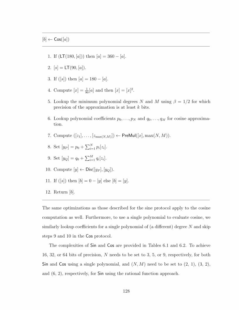
[b] Cos([a])

1. If (LT(180, [a])) then [a] = 360� [a].

2. [s] = LT(90, [a]).

3. If ([s]) then [a] = 180� [a].

4. Compute [x] = 1

90

[a] and then [x] = [x]2.

5. Lookup the minimum polynomial degrees N and M using � = 1/2 for whichprecision of the approximation is at least k bits.


, . . ., pN

and q0

, . . ., qM

for cosine approxima-tion.

7. Compute ([z1

], . . . , [zmax(N,M)

]) PreMul([x],max(N,M)).

8. Set [yP

] = p0

+P

N

i=1

pi

[zi

].

9. Set [yQ

] = q0

+P

M

i=1

qi

[zi

].

10. Compute [y] Div([yP

], [yQ

]).

11. If ([s]) then [b] = 0� [y] else [b] = [y].

12. Return [b].

The same optimizations as those described for the sine protocol apply to the cosine

computation as well. Furthermore, to use a single polynomial to evaluate cosine, we

similarly lookup coe�cients for a single polynomial of (a di↵erent) degree N and skip

steps 9 and 10 in the Cos protocol.

The complexities of Sin and Cos are provided in Tables 6.1 and 6.2. To achieve

16, 32, or 64 bits of precision, N needs to be set to 3, 5, or 9, respectively, for both

Sin and Cos using a single polynomial, and (N,M) need to be set to (2, 1), (3, 2),

and (6, 2), respectively, for Sin using the rational function approach.

128

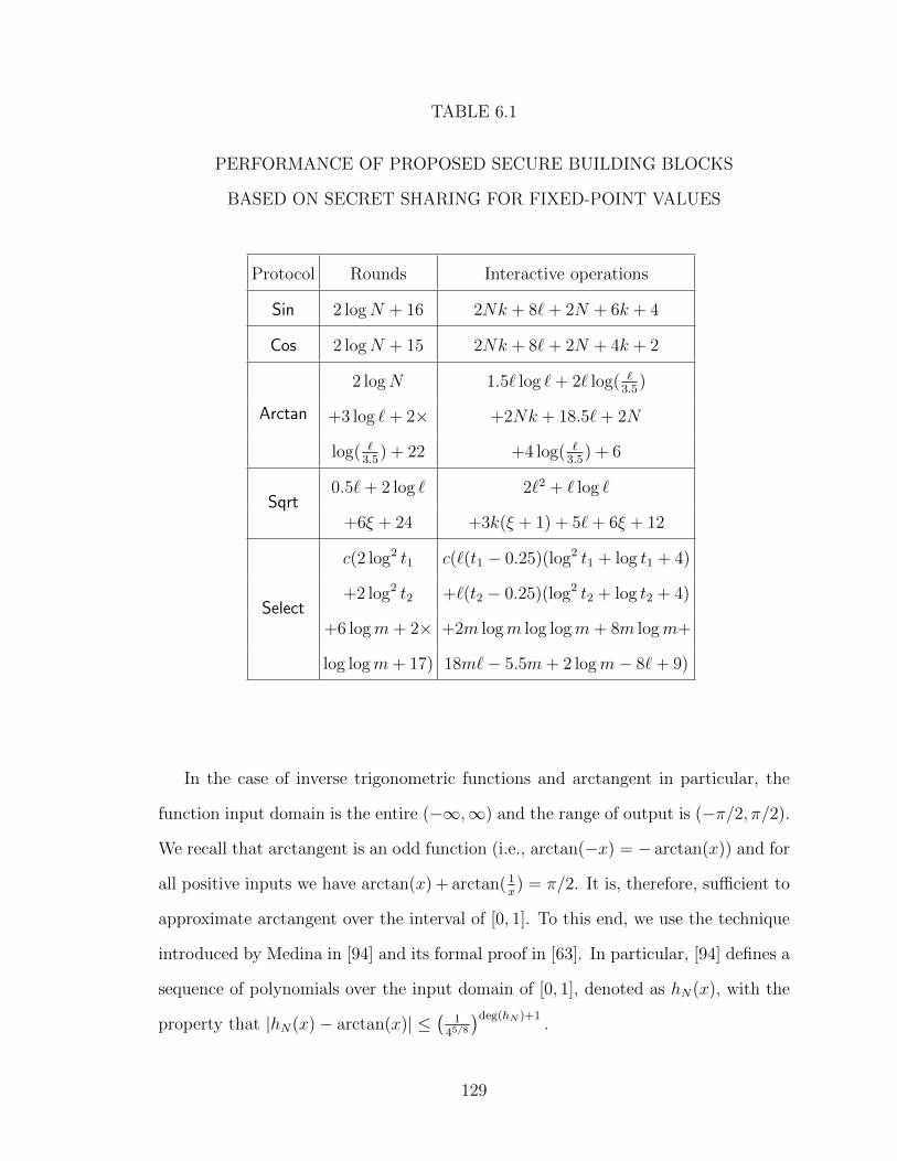
TABLE 6.1

PERFORMANCE OF PROPOSED SECURE BUILDING BLOCKS

BASED ON SECRET SHARING FOR FIXED-POINT VALUES

Protocol Rounds Interactive operations

Sin 2 logN + 16 2Nk + 8`+ 2N + 6k + 4

Cos 2 logN + 15 2Nk + 8`+ 2N + 4k + 2

Arctan

2 logN 1.5` log `+ 2` log( `

3.5

)

+3 log `+ 2⇥ +2Nk + 18.5`+ 2N

log( `

3.5

) + 22 +4 log( `

3.5

) + 6

Sqrt0.5`+ 2 log ` 2`2 + ` log `

+6⇠ + 24 +3k(⇠ + 1) + 5`+ 6⇠ + 12

Select

c(2 log2 t1

c(`(t1

� 0.25)(log2 t1

+ log t1

+ 4)

+2 log2 t2

+`(t2

� 0.25)(log2 t2

+ log t2

+ 4)

+6 logm+ 2⇥ +2m logm log logm+ 8m logm+

log logm+ 17) 18m`� 5.5m+ 2 logm� 8`+ 9)

In the case of inverse trigonometric functions and arctangent in particular, the

function input domain is the entire (�1,1) and the range of output is (�⇡/2, ⇡/2).

We recall that arctangent is an odd function (i.e., arctan(�x) = � arctan(x)) and for

all positive inputs we have arctan(x) + arctan( 1x

) = ⇡/2. It is, therefore, su�cient to

approximate arctangent over the interval of [0, 1]. To this end, we use the technique

introduced by Medina in [94] and its formal proof in [63]. In particular, [94] defines a

sequence of polynomials over the input domain of [0, 1], denoted as hN

(x), with the

property that |hN

(x)� arctan(x)| �

1

4

5/8

�deg(h

N

)+1

.

129

TABLE 6.2

PERFORMANCE OF PROPOSED SECURE BUILDING BLOCKS

BASED ON GARBLED CIRCUIT FOR FIXED-POINT VALUES

Protocol XOR gates Non-XOR gates

Sin

(max(N,M) +N +M + 2) (max(N,M) +N +M + 2)

⇥(4`2 � 4`) + 7`2 ⇥(2`2 � `) + 3`2

+4`(N +M) + 31` +`(N +M) + 11`

Cos

(max(N,M) +N +M + 1) (max(N,M) +N +M

⇥(4`2 � 4`) + 7`2 ⇥(2`2 � `) + 3`2

+4`(N +M) + 31` +`(N +M) + 11`

Arctan 8N`2 + 3`2 � 4N`+ 43` 4N`2 + `2 �N`+ 15`

Sqrt12⇠`2 + 12.5`2 � k2 6⇠`2 + 6.5`2 � k2

+`k � 8⇠`� 7.5`+ k � 2 +`k � 2⇠`� 0.5`+ k � 4

Select

c(1.5t1

`(log2 t1

+ log t1

+ 4) c(0.5t1

`(log2 t1

+ log t1

+ 4)

+1.5t2

`(log2 t2

+ log t2

+ 4) +0.5t2

`(log2 t2

+ log t2

+ 4)

+(2`+ 20.5)m logm+m +(4`+ 5)m logm+m

+12.5m`� 6 logm� 8`) +4m`+ (2`� 1) logm)

We use this formula to determine the degreeN for any k-bit precision. This degree

N is logarithmic with respect to the desired precision. Afterwards, the coe�cients of

hN

(x) are computed from the recursive definitions in [94]. We choose this approach

over other alternatives such as [68] for its e�ciency. As an example, in [68] the authors

propose to divide [0,1) into s+1 segments for some value of s and perform a search

to discover in which interval the input falls. Afterwards, the input is transformed into

130

another variable (involving division) whose value is guaranteed to be within a small

fixed interval and arctangent of this new variable is approximated using standard

polynomial approximation techniques. In this approach, the search can be performed

using binary search trees whose secure realization is non-trivial or alternatively will

involve s steps. This extra computation makes the overall performance of the solution

in [68] worse than that of [94]’s approach used here. Another candidate for arctangent

evaluation is the well-known Taylor series of arctangent. However, Taylor series

provides possibly reasonable precision if the input is bound to be very close to one

point from the input domain, which we cannot assume. In addition, arctangent

Taylor series converges very slowly. For example, for a three decimal precision on

inputs around 0.95 Taylor series requires a polynomial of degree 57, whereas [94]’s

approach requires a 7th-degree polynomial [63]. Our secure protocol to approximate

arctangent based on the approach from [94] is given next:

[b] Arctan([a])

1. Compute [s] LT([a], 0).

2. If ([s]) then [x] = 0� [a] else [x] = [a].

3. Compute [c] LT(1, [x]).

4. If ([c]) then [d] = ⇡/2, [y] Div(1, [x]); else [d] = 0, [y] = [x].

5. Lookup the minimum polynomial degree N for which precision of the approxi-mation is at least k bits.


, . . ., pN

for arctangent approximation from[94].

7. Compute ([z1

], . . . , [zN

]) PreMul([y], N).

8. Set [z] = p0

+P

N

i=1

pi

[zi

].

131

9. If ([c]) then [z] = [d]� [z] else [z] = [d] + [z].

10. If ([s]) then [b] = 0� [z] else [b] = [z].

11. Return [b].

The complexity of this protocol can be found in Tables 6.1 and 6.2.

6.5.1.2 Square Root

We now proceed with the square root computation defined by the interface [b]

Sqrt([a]), where a and b are fixed-point values to cover the general case.

Secure multi-party computation of the square root based on secret sharing has

been treated by Liedel in [88]. The approach is based on the Goldschmidt’s algo-

rithm, which is faster than the Newton-Raphson’s method. However, to eliminate

the accumulated errors, the last iteration of the algorithm is replaced with the self-

correcting iteration of the Newton-Raphson’s method. For an `-bit input a with k

bits after the radix point, this protocol uses 2`2 + ` log ` + 3k(⇠ + 1) + 5` + 6⇠ + 12

interactive operations in 0.5` + 2 log ` + 6⇠ + 24 rounds, where ` is assumed to be

a power of 2 and ⇠ = dlog2

(`/5.4)e is the number of algorithm iterations. For the

purposes of this work, we use the protocol from [88] for the secret sharing setting. We

also optimize the computation to be used with garbled circuit based on the specifics

of that technique as described next.

Goldschmidt’s method starts by computing an initial approximation for 1pa

, de-

noted by b0

, that satisfies 1

2

ab20

< 3

2

. It then proceeds in iterations increasing the

precision of the approximation with each consecutive iteration. To approximate 1pa

,

[88] uses an e�cient method (a linear equation) that expects that input a is in the

range [12

, 1). Thus, there is a need to first normalize a to a0 such that 1

2

a0 < 1 and

a = a0 · 2w. Note that 1pa

= 1pa

0

p2�w, therefore, once we approximate 1p

a

0 , we can

multiply it byp2�w to determine an approximation of 1p

a

.

132

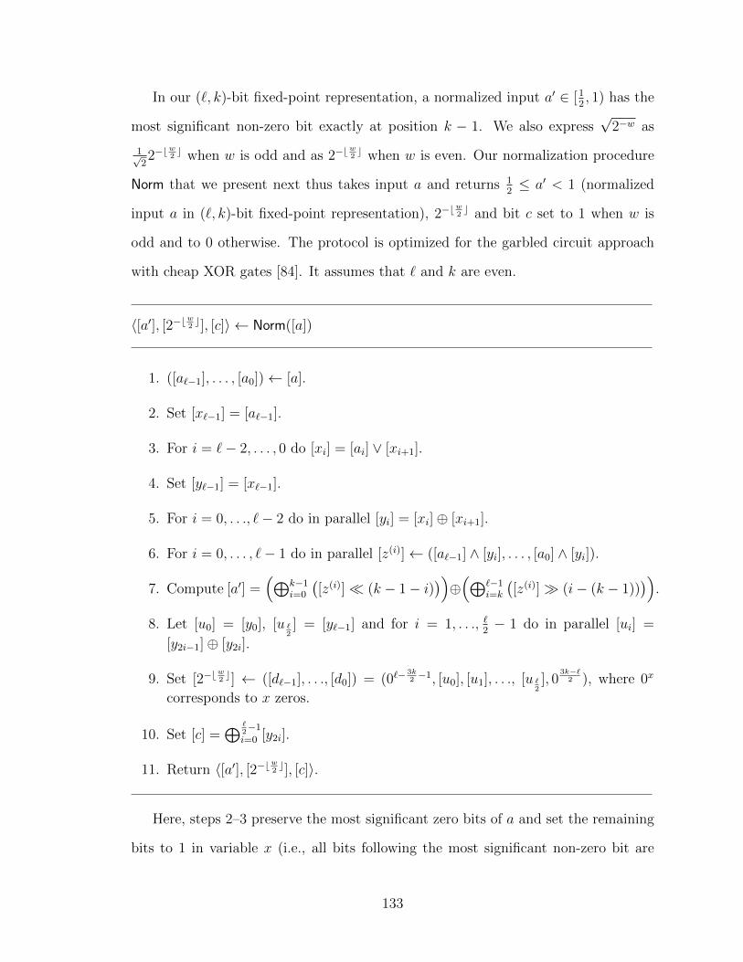
In our (`, k)-bit fixed-point representation, a normalized input a0 2 [12

, 1) has the

most significant non-zero bit exactly at position k � 1. We also expressp2�w as

1p2

2�bw

2 c when w is odd and as 2�bw

2 c when w is even. Our normalization procedure

Norm that we present next thus takes input a and returns 1

2

a0 < 1 (normalized

input a in (`, k)-bit fixed-point representation), 2�bw

2 c and bit c set to 1 when w is

odd and to 0 otherwise. The protocol is optimized for the garbled circuit approach

with cheap XOR gates [84]. It assumes that ` and k are even.

h[a0], [2�bw

2 c], [c]i Norm([a])

1. ([a`�1

], . . . , [a0

]) [a].

2. Set [x`�1

] = [a`�1

].

3. For i = `� 2, . . . , 0 do [xi

] = [ai

] _ [xi+1

].

4. Set [y`�1

] = [x`�1

].

5. For i = 0, . . ., `� 2 do in parallel [yi

] = [xi

]� [xi+1

].

6. For i = 0, . . . , `� 1 do in parallel [z(i)] ([a`�1

] ^ [yi

], . . . , [a0

] ^ [yi

]).

7. Compute [a0] =⇣L

k�1

i=0

�[z(i)]⌧ (k � 1� i)

�⌘�⇣L

`�1

i=k

�[z(i)]� (i� (k � 1))

�⌘.

8. Let [u0

] = [y0

], [u `

2] = [y

`�1

] and for i = 1, . . ., `

2

� 1 do in parallel [ui

] =

[y2i�1

]� [y2i

].

9. Set [2�bw

2 c] ([d`�1

], . . ., [d0

]) = (0`�3k2 �1, [u

0

], [u1

], . . ., [u `

2], 0

3k�`

2 ), where 0x

corresponds to x zeros.

10. Set [c] =L `

2�1

i=0

[y2i

].

11. Return h[a0], [2�bw

2 c], [c]i.

Here, steps 2–3 preserve the most significant zero bits of a and set the remaining

bits to 1 in variable x (i.e., all bits following the most significant non-zero bit are

133

1). Steps 4–5 compute y as a vector with the most significant non-zero bit of a set

to 1 and all other bits set to 0. On step 6, each vector z(i) is either filled with 0s

or set to a depending on the ith bit of y (thus, all but one z(i) can be non-zero).

Step 7 computes the normalized value of a by aggregating all vectors z(i) shifted an

appropriate number of positions. Here operation x⌧ y shifts `-bit representation of

x y positions to the left by discarding y most significant bits of x and appending y 0s

in place of least significant bits. Similarly, x� y shifts x to the right by prepending

y 0s in place of most significant bits and discarding y least significant bits of x. Note

that we can use cheap XOR gates for this aggregation operation because at most one

yi

can take a non-zero value.

Steps 8 and 9 compute [2�bw

2 c]. Because a pair of consecutive i’s results in the

same value of w, we first combine the pairs on step 8 and shift them in place on step

9. As before, we can use cheap XOR and free shift operations to accomplish this

task because at most one yi

is set. Lastly, step 10 computes the bit c, which is set

by combining all flags yi

’s at odd distances from k � 1.

Note that for simplicity of exposition, we AND and XOR all bits in steps 6 and

7. There is, however, no need to compute the AND for the bits discarded in step

7 or compute the XOR with newly appended or prepended 0s. We obtain that this

protocol can be implemented as a circuit using 0.5`2 � k2 + `k + 1.5` � 4 non-XOR

and 0.5`2 � k2 + `k + 0.5`� 3 XOR gates.

Once we determine normalized input a0, Liedel [88] approximates 1pa

0 , denoted by

b00

, by a linear equation b00

= ↵a0 + �, where ↵ and � are precomputed. The values

of these coe�cients are set to ↵ = �0.8099868542 and � = 1.787727479 in [88] to

compute an initial approximation b00

with almost 5.5 bits of precision (when a0 is in the

range [12

, 1)). We then use b00

to compute b0

that approximates 1pa

as described above.

After the initialization, Goldschmidt’s algorithm sets g0

= xb0

and h0

= 0.5b0

and

proceeds in ⇠ iterations that compute: gi+1

= gi

(1.5�gi

hi

), hi+1

= hi

(1.5�gi

hi

). The

134

last iteration is replaced with one iteration of Newton-Raphson’s method to eliminate

accumulated errors that computes the following: hi+1

= hi

(1.5�0.5ah2

i

). This gives us

the following square root protocol, which we present optimized for the garbled circuit.

[b] Sqrt([a])

1. Let ⇠ = dlog2

( `

5.4

)e.

2. Execute h[a0], [2�bw

2 c], [c]i Norm([a]).

3. Let ↵ = �0.8099868542, � = 1.787727479 and compute [b00

] = ↵ · [a0] + �.

4. Compute [b0

] =⇣⇣

[c] ^ 1p2

⌘� ¬[c]

⌘· [2�bw

2 c] · [b00

].

5. Compute [g0

] = [a] · [b0

] and [h0

] = ([b0

]� 1).

6. For i = 0, . . . , ⇠ � 2 do

(a) [x] = 1.5� [gi

] · [hi

].

(b) if (i < ⇠ � 2) then [gi+1

] = [gi

] · [x].

(c) [hi+1

] = [hi

] · [x].

7. Compute [h⇠

] = [h⇠�1

](1.5� ([a] · [h⇠�1

]2 � 1)).

8. Return [b] = [h⇠

].

Here multiplication by 0.5 is replaced by shift to the right by 1 bit that has no

cost. Complexity of this protocol can be found in Table 6.2.

6.5.1.3 Selection

There are multiple ways to find the fth smallest element of a set. The most

straightforward method is to obliviously sort the input set and return the fth element

of the sorted set. This approach is often beneficial when the input set is small. It is

135

usually faster to use a selection algorithm, and the goal of this section is to design

an oblivious selection protocol for finding the fth smallest element of a set.

The regular non-oblivious selection algorithms run in O(m) time on m-element

sets. We considered both deterministic and probabilistic algorithms and settled on

a probabilistic algorithm that performs the best in the secure setting in practice.

Its complexity is O(m logm) due to the use of data-oblivious compaction. Goodrich

[67] proposed a probabilistic oblivious selection algorithm that works in linear time.

Our starting point, however, is a di↵erent simpler algorithm that performs well in

practice. Our algorithm proceeds by scanning through the input set and selects each

element with probability c1pm

for some constant c1

. The expected number of selected

elements is O(pm). The algorithm then sorts the selected elements and determines

two elements x and y between which the fth smallest element is expected to lie

based on f , m, and the number of selected elements. Afterwards, we scan the input

set again retrieving all elements with values between x and y and simultaneously

computing the ranks of x and y in the input set; let rx

and ry

denote the ranks. The

expected number of retrieved elements is O(pm). We sort the retrieved elements

and return the element at position f � rx

in the sorted set. Let t1

denote the number

of elements randomly selected in the beginning of the algorithm and t2

denote the

number of elements with values between x and y.

Because of the randomized nature of our algorithm, it can fail at multiple points

of its execution. In particular, if the number of elements selected in the beginning of

the algorithm is too large or too small (and the performance guarantees cannot be

met), we abort. Similarly, if the number of the retrieved elements that lie between

x and y is too small, we abort. Lastly, if f does not lie between the ranks of x and

y, the fth smallest element will not be among the retrieved elements and we abort.

It can be shown using the union bound that all of the above events happen with a

probability negligible in the input size. By using the appropriate choice of constants

136

we can also ensure that faults are very rare in practice (see below). Thus, in the rare

event of failure, the algorithm needs to be restarted using new random choices, and

the expected number of times the algorithm is to be executed is slightly above 1.

Our protocol Select is given below. Compared to the algorithm structure outlined

above, we need to ensure high probability of success through the appropriate selection

of x and y as well as some constant parameters. We also need to ensure that the

execution can proceed obliviously without compromising private data. To achieve

this, we use three constants c1

, c2

, and c. The value of c1

influences the probability

with which an element is selected in the beginning of the algorithm. The value

of c influences the distance between x and y in the set of t1

selected elements. In

particular, we first determine the position where f is expected to be positioned among

the t1

selected elements as (ft1

)/m. We then choose x to be c elements before that

position and choose y to be 3c elements after that position. Lastly, c2

is used to

control the size of t2

. When t2

is too small due to the random choices made during

the execution, we abort.

To turn this logic into a data-oblivious protocol, we resort to secure and oblivious

set operations. In particular, after we mark each element of the input set as selected

or not selected, we use data-oblivious compaction to place all selected elements in

the beginning of the set. Similarly, we use data-oblivious sorting to sort t1

and t2

elements.

[b] Select(h[a1

], . . . , [am

]i, f)

1. Set constants c1

, c2

, and c; also set n =pm, [t

1

] = 0, and [t2

] = 0.

2. For i = 1, . . . ,m set [bi

] = 0.

3. For i = 1, . . . ,m do in parallel

(a) Generate random [ri

] 2 Zn

.

137

(b) If LT([ri

], c1

) then [bi

] = 1.

4. For i = 1, . . . ,m do [t1

] = [t1

] + [bi

].

5. Open the value of t1

.

6. If ((t1

> 2c1

n) _ (t1

< 1

2

c1

n)) then abort.

7. Execute h[a01

], . . . , [a0m

]i Comp(h[b1

], [a1

] ^ [b1

]i, . . . , h[bm

], [am

] ^ [bm

]i).

8. Execute h[a001

], . . . , [a00t1]i Sort([a0

1

], . . . , [a0t1]).

9. Compute k as the closest integer to (ft1

)/m.

10. If (k � c < 1) then [x] Min([a1

], . . . , [am

]); else [x] = [a00k�c

].

11. If (k + 3c > t1

) then [y] Max([a1

], . . . , [am

]); else [y] = [a00k+3c

].

12. Set [rx

] = 0 and [ry

] = 0.

13. For i = 1, . . . ,m do in parallel [gi

] = LT([ai

], [x]) and [g0i

] = LT([ai

], [y]).

14. For i = 1, . . . ,m do in parallel [b0i

] = ¬[gi

] ^ [g0i

].

15. For i = 1, . . . ,m do [rx

] = [rx

] + [gi

] and [t2

] = [t2

] + [b0i

].

16. Open the values of rx

and t2

.

17. If ((t2

< 4cc2

n) _ ((f � rx

) < 0) _ ((f � rx

) > t2

)) then abort.

18. Execute h[d1

], . . . , [dm

]i Comp(h[b01

], [a1

] ^ [b01

]i, . . . , h[b0m

], [am

] ^ [b0m

]i).

19. Execute h[d01

], . . . , [d0t2]i Sort([d

1

], . . . , [dt2 ]).

20. Return [b] = [d0f�r

x

].

Note that because maximum and minimum functions are evaluated on the same

set, we reduce the overhead of evaluating them simultaneously compared to evaluating

them individually. In particular, when min and max functions are evaluated in a tree-

like fashion on an m-element set, we use the m/2 comparison in the first layer to set

138

both minimum and maximum elements of each pair using the same cost as evaluating

only one of them. The rest is evaluated as before, and we save about 1/2 overhead

of one of min or max.

Complexity of this protocol is given in Tables 6.1 and 6.2 as a function of param-

eters m, t1

, t2

, c, and bitlength `. The expected value of t1

is c1

pm, the expected

value of t2

is (4cpm)/c

1

, and c indicates the average number of times the algorithm

needs to be invoked, which is a constant slightly larger than 1 (see below).

We experimentally determined the best values for c1

, c2

, and c for di↵erent values

of n to ensure high success of the algorithm. Based on the experiments, we recom-

mend to set c1

= 2, c2

= 2, and c = 10. Using these values, the probability of the

protocol’s failure on a single run is at most a few percent up to input size 10,000.

With larger input sizes, a larger value of c might be preferred.

Unlike all other protocols presented in this work, three values t1

, t2

, and rx

pri-

vately computed in Select are opened during its execution. Thus, to guarantee se-

curity, we need to show that these values are independent of the private input set

and result in no information leakage. First, observe that the value of t1

is computed

purely based on random choices made in step 3(a) of the protocol. Thus, its value

is data-independent. Second, the rank of x; rx

, is determined by random choices,

but not the data values themselves. Similarly, the value of t2

depends only on the

ranks of the randomly chosen pivots, but not on the actual data values. Therefore,

execution is data-oblivious and security is maintained.

6.6 Secure Fingerprint Recognition

We are now ready to proceed with the description of our solutions for secure

fingerprint recognition using the building blocks introduced in Sections 3.2.1 and

6.5.1. We provide three constructions, one for each fingerprint recognition approach

described in Section 6.3.

139

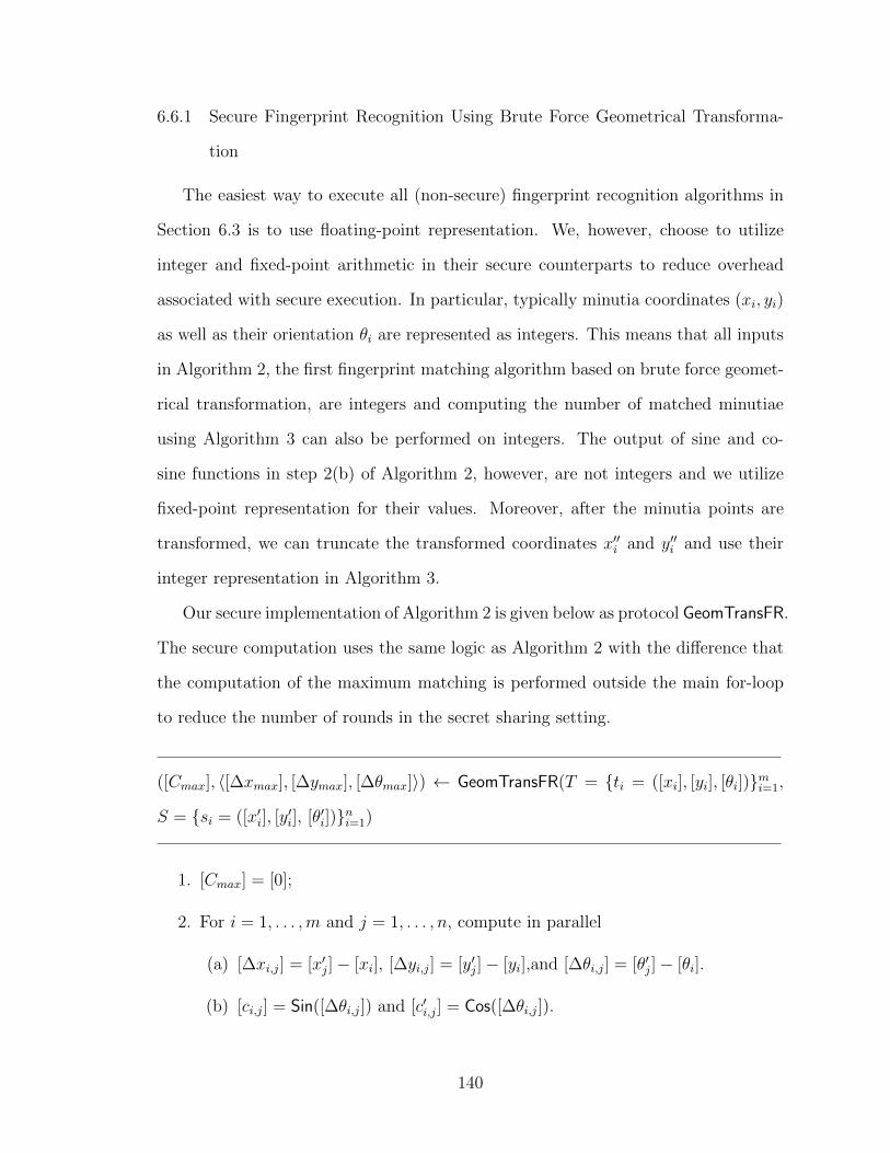
6.6.1 Secure Fingerprint Recognition Using Brute Force Geometrical Transforma-

tion

The easiest way to execute all (non-secure) fingerprint recognition algorithms in

Section 6.3 is to use floating-point representation. We, however, choose to utilize

integer and fixed-point arithmetic in their secure counterparts to reduce overhead

associated with secure execution. In particular, typically minutia coordinates (xi

, yi

)

as well as their orientation ✓i

are represented as integers. This means that all inputs

in Algorithm 2, the first fingerprint matching algorithm based on brute force geomet-

rical transformation, are integers and computing the number of matched minutiae

using Algorithm 3 can also be performed on integers. The output of sine and co-

sine functions in step 2(b) of Algorithm 2, however, are not integers and we utilize

fixed-point representation for their values. Moreover, after the minutia points are

transformed, we can truncate the transformed coordinates x00i

and y00i

and use their

integer representation in Algorithm 3.

Our secure implementation of Algorithm 2 is given below as protocol GeomTransFR.

The secure computation uses the same logic as Algorithm 2 with the di↵erence that

the computation of the maximum matching is performed outside the main for-loop

to reduce the number of rounds in the secret sharing setting.

([Cmax

], h[�xmax

], [�ymax

], [�✓max

]i) GeomTransFR(T = {ti

= ([xi

], [yi

], [✓i

])}mi=1

,

S = {si

= ([x0i

], [y0i

], [✓0i

])}ni=1

)

1. [Cmax

] = [0];

2. For i = 1, . . . ,m and j = 1, . . . , n, compute in parallel

(a) [�xi,j

] = [x0j

]� [xi

], [�yi,j

] = [y0j

]� [yi

],and [�✓i,j

] = [✓0j

]� [✓i

].

(b) [ci,j

] = Sin([�✓i,j

]) and [c0i,j

] = Cos([�✓i,j

]).

140

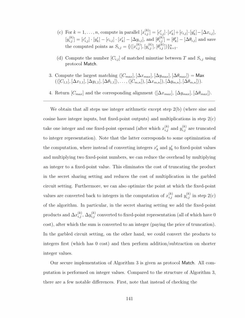
(c) For k = 1, . . . , n, compute in parallel [x(k)

i,j

] = [c0i,j

]· [x0k

]+[ci,j

]· [y0k

]� [�xi,j

],

[y(k)i,j

] = [c0i,j

] · [y0k

]� [ci,j

] · [x0k

]� [�yi,j

], and [✓(k)i,j

] = [✓0k

]� [�✓i,j

] and save

the computed points as Si,j

= {([x(k)

i,j

], [y(k)i,j

], [✓(k)i,j

])}nk=1

.

(d) Compute the number [Ci,j

] of matched minutiae between T and Si,j

usingprotocol Match.

3. Compute the largest matching h[Cmax

], [�xmax

], [�ymax

], [�✓max

]i = Max(h[C

1,1

], [�x1,1

], [�y1,1

], [�✓1,1

]i, . . . , h[Cm,n

]), [�xm,n

]), [�ym,n

], [�✓m,n

]i).

4. Return [Cmax

] and the corresponding alignment h[�xmax

], [�ymax

], [�✓max

]i.

We obtain that all steps use integer arithmetic except step 2(b) (where sine and

cosine have integer inputs, but fixed-point outputs) and multiplications in step 2(c)

take one integer and one fixed-point operand (after which x(k)

i,j

and y(k)i,j

are truncated

to integer representation). Note that the latter corresponds to some optimization of

the computation, where instead of converting integers x0k

and y0k

to fixed-point values

and multiplying two fixed-point numbers, we can reduce the overhead by multiplying

an integer to a fixed-point value. This eliminates the cost of truncating the product

in the secret sharing setting and reduces the cost of multiplication in the garbled

circuit setting. Furthermore, we can also optimize the point at which the fixed-point

values are converted back to integers in the computation of x(k)

i,j

and y(k)i,j

in step 2(c)

of the algorithm. In particular, in the secret sharing setting we add the fixed-point

products and �x(k)

i,j

, �y(k)i,j

converted to fixed-point representation (all of which have 0

cost), after which the sum is converted to an integer (paying the price of truncation).

In the garbled circuit setting, on the other hand, we could convert the products to

integers first (which has 0 cost) and then perform addition/subtraction on shorter

integer values.

Our secure implementation of Algorithm 3 is given as protocol Match. All com-

putation is performed on integer values. Compared to the structure of Algorithm 3,

there are a few notable di↵erences. First, note that instead of checking the

141

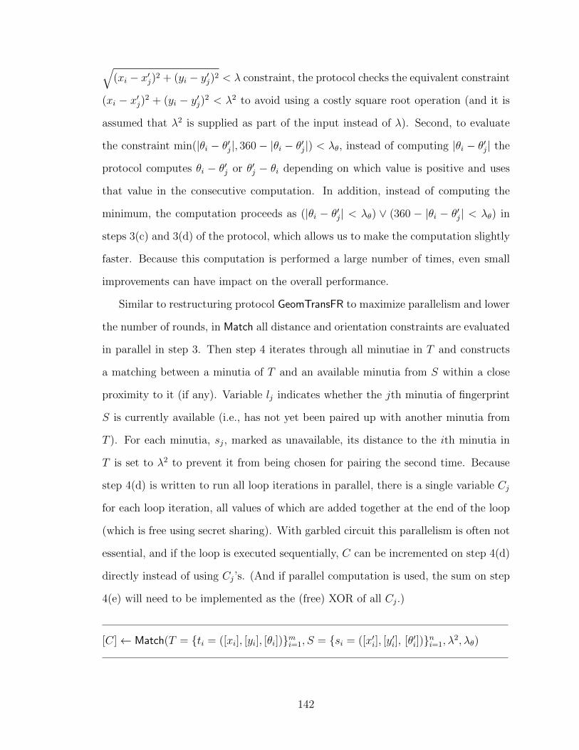
q(x

i

� x0j

)2 + (yi

� y0j

)2 < � constraint, the protocol checks the equivalent constraint

(xi

� x0j

)2 + (yi

� y0j

)2 < �2 to avoid using a costly square root operation (and it is

assumed that �2 is supplied as part of the input instead of �). Second, to evaluate

the constraint min(|✓i

� ✓0j

|, 360 � |✓i

� ✓0j

|) < �✓

, instead of computing |✓i

� ✓0j

| the

protocol computes ✓i

� ✓0j

or ✓0j

� ✓i

depending on which value is positive and uses

that value in the consecutive computation. In addition, instead of computing the

minimum, the computation proceeds as (|✓i

� ✓0j

| < �✓

) _ (360 � |✓i

� ✓0j

| < �✓

) in

steps 3(c) and 3(d) of the protocol, which allows us to make the computation slightly

faster. Because this computation is performed a large number of times, even small

improvements can have impact on the overall performance.

Similar to restructuring protocol GeomTransFR to maximize parallelism and lower

the number of rounds, in Match all distance and orientation constraints are evaluated

in parallel in step 3. Then step 4 iterates through all minutiae in T and constructs

a matching between a minutia of T and an available minutia from S within a close

proximity to it (if any). Variable lj

indicates whether the jth minutia of fingerprint

S is currently available (i.e., has not yet been paired up with another minutia from

T ). For each minutia, sj

, marked as unavailable, its distance to the ith minutia in

T is set to �2 to prevent it from being chosen for pairing the second time. Because

step 4(d) is written to run all loop iterations in parallel, there is a single variable Cj

for each loop iteration, all values of which are added together at the end of the loop

(which is free using secret sharing). With garbled circuit this parallelism is often not

essential, and if the loop is executed sequentially, C can be incremented on step 4(d)

directly instead of using Cj

’s. (And if parallel computation is used, the sum on step

4(e) will need to be implemented as the (free) XOR of all Cj

.)

[C] Match(T = {ti

= ([xi

], [yi

], [✓i

])}mi=1

, S = {si

= ([x0i

], [y0i

], [✓0i

])}ni=1

,�2,�✓

)

142

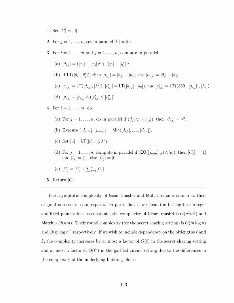
1. Set [C] = [0].

2. For j = 1, . . . , n, set in parallel [lj

] = [0].

3. For i = 1, . . . ,m and j = 1, . . . , n, compute in parallel

(a) [di,j

] = ([xi

]� [x0j

])2 + ([yi

]� [y0j

])2.

(b) If LT([✓i

], [✓0j

]), then [ai,j

] = [✓0j

]� [✓i

], else [ai,j

] = [✓i

]� [✓0j

].

(c) [ci,j

] = LT([di,j

], [�2]), [c0i,j

] = LT([ai,j

], [�✓

]), and [c00i,j

] = LT((360�[ai,j

]), [�✓

]).

(d) [vi,j

] = [ci,j

] ^ ([c0i,j

] _ [c00i,j

]).

4. For i = 1, . . . ,m, do

(a) For j = 1, . . . , n, do in parallel if ([lj

] _ ¬[vi,j

]), then [di,j

] = �2.

(b) Execute ([dmin

], [jmin

]) = Min([di,1

], . . . , [di,n

]).

(c) Set [u] = LT([dmin

],�2).

(d) For j = 1, . . . , n, compute in parallel if (EQ([jmin

], j)^ [u]), then [Cj

] = [1]and [l

j

] = [1], else [Cj

] = [0].

(e) [C] = [C] +P

n

j=1

[Cj

].

5. Return [C].

The asymptotic complexity of GeomTransFR and Match remains similar to their

original non-secure counterparts. In particular, if we treat the bitlength of integer

and fixed-point values as constants, the complexity of GeomTransFR is O(n2m2) and

Match is O(nm). Their round complexity (for the secret sharing setting) is O(m log n)

and O(m log n), respectively. If we wish to include dependency on the bitlengths ` and

k, the complexity increases by at most a factor of O(`) in the secret sharing setting

and at most a factor of O(`2) in the garbled circuit setting due to the di↵erences in

the complexity of the underlying building blocks.

143

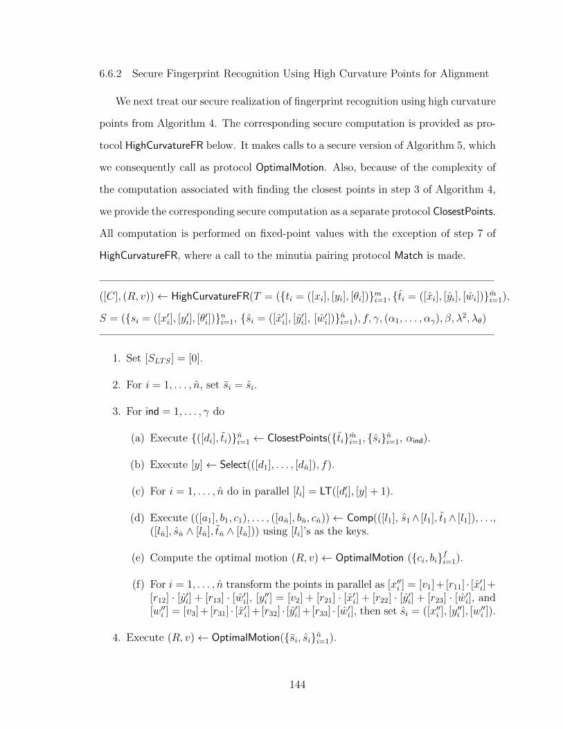
6.6.2 Secure Fingerprint Recognition Using High Curvature Points for Alignment

We next treat our secure realization of fingerprint recognition using high curvature

points from Algorithm 4. The corresponding secure computation is provided as pro-

tocol HighCurvatureFR below. It makes calls to a secure version of Algorithm 5, which

we consequently call as protocol OptimalMotion. Also, because of the complexity of

the computation associated with finding the closest points in step 3 of Algorithm 4,

we provide the corresponding secure computation as a separate protocol ClosestPoints.

All computation is performed on fixed-point values with the exception of step 7 of

HighCurvatureFR, where a call to the minutia pairing protocol Match is made.

([C], (R, v)) HighCurvatureFR(T = ({ti

= ([xi

], [yi

], [✓i

])}mi=1

, {ti

= ([xi

], [yi

], [wi

])}mi=1

),

S = ({si

= ([x0i

], [y0i

], [✓0i

])}ni=1

, {si

= ([x0i

], [y0i

], [w0i

])}ni=1

), f, �, (↵1

, . . . ,↵�

), �,�2,�✓

)

1. Set [SLTS

] = [0].

2. For i = 1, . . . , n, set si

= si

.

3. For ind = 1, . . . , � do

(a) Execute {([di

], ti

)}ni=1

ClosestPoints({ti

}mi=1

, {si

}ni=1

, ↵ind).

(b) Execute [y] Select(([d1

], . . . , [dn

]), f).

(c) For i = 1, . . . , n do in parallel [li

] = LT([d0i

], [y] + 1).

(d) Execute (([a1

], b1

, c1

), . . . , ([an

], bn

, cn

)) Comp(([l1

], s1

^ [l1

], t1

^ [l1

]), . . .,([l

n

], sn

^ [ln

], tn

^ [ln

])) using [li

]’s as the keys.

(e) Compute the optimal motion (R, v) OptimalMotion ({ci

, bi

}fi=1

).

(f) For i = 1, . . . , n transform the points in parallel as [x00i

] = [v1

]+ [r11

] · [x0i

]+[r

12

] · [y0i

] + [r13

] · [w0i

], [y00i

] = [v2

] + [r21

] · [x0i

] + [r22

] · [y0i

] + [r23

] · [w0i

], and[w00

i

] = [v3

]+ [r31

] · [x0i

]+ [r32

] · [y0i

]+ [r33

] · [w0i

], then set si

= ([x00i

], [y00i

], [w00i

]).

4. Execute (R, v) OptimalMotion({si

, si

}ni=1

).

144

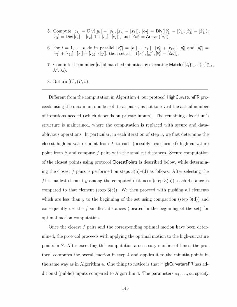
5. Compute [c1

] = Div([y2

] � [y1

], [x2

] � [x1

]), [c2

] = Div([y02

] � [y01

], [x02

] � [x01

]),[c

3

] = Div([c1

]� [c2

], 1 + [c1

] · [c2

]), and [�✓] = Arctan([c3

]).

6. For i = 1, . . . , n do in parallel [x00i

] = [v1

] + [r11

] · [x0i

] + [r12

] · [y0i

] and [y00i

] =[v

2

] + [r21

] · [x0i

] + [r22

] · [y0i

], then set si

= ([x00i

], [y00i

], [✓0i

]� [�✓]).

7. Compute the number [C] of matched minutiae by executingMatch ({ti

}mi=1

, {si

}ni=1

,�2,�

✓

).

8. Return [C], (R, v).

Di↵erent from the computation in Algorithm 4, our protocol HighCurvatureFR pro-

ceeds using the maximum number of iterations �, as not to reveal the actual number

of iterations needed (which depends on private inputs). The remaining algorithm’s

structure is maintained, where the computation is replaced with secure and data-

oblivious operations. In particular, in each iteration of step 3, we first determine the

closest high-curvature point from T to each (possibly transformed) high-curvature

point from S and compute f pairs with the smallest distances. Secure computation

of the closest points using protocol ClosestPoints is described below, while determin-

ing the closest f pairs is performed on steps 3(b)–(d) as follows. After selecting the

fth smallest element y among the computed distances (step 3(b)), each distance is

compared to that element (step 3(c)). We then proceed with pushing all elements

which are less than y to the beginning of the set using compaction (step 3(d)) and

consequently use the f smallest distances (located in the beginning of the set) for

optimal motion computation.

Once the closest f pairs and the corresponding optimal motion have been deter-

mined, the protocol proceeds with applying the optimal motion to the high-curvature

points in S. After executing this computation a necessary number of times, the pro-

tocol computes the overall motion in step 4 and applies it to the minutia points in

the same way as in Algorithm 4. One thing to notice is that HighCurvatureFR has ad-

ditional (public) inputs compared to Algorithm 4. The parameters ↵1

, . . .,↵�

specify

145

bounding box sizes for the purposes of closest points computation in step 3(a) (see

below). The remaining new parameters �2, �✓

and � are made explicit as inputs to

the minutia pairing protocol Match and the scaling factor in distance computation

(step 3 of Algorithm 4).

The protocol ClosestPoints below takes two sets of points ti

’s and si

’s (represented

using three coordinates each) and for each point si

returns the closest element among

the ti

’s and the corresponding distance. As mentioned in Section 6.3.2, the TICP

algorithm on which our construction builds uses the bounding box approach to elim-

inate errors during this computation. In particular, only points within a certain

distance from a point are considered, and the maximum allowable distance (i.e., the

bounding box size) is denoted by ↵i

in the ith iteration of HighCurvatureFR or Algo-

rithm 4. The sizes of the bounding boxes become smaller with each iteration as the

two sets of points become closer to each other. When we make a call to ClosestPoints,

we pass a single bounding box size for the current iteration and that parameter is

denoted as ↵ in the interface of ClosestPoints.

{([di

], ti

)}ni=1

ClosestPoints({ti

= (xi

, yi

, wi

)}mi=1

, {si

= (x0i

, y0i

, w0i

)}ni=1

,↵, �)

1. For i = 1, . . . , n and for j = 1, . . . , m do in parallel

(a) Set [d(i,j)

] = Sqrt([xj

]� [x0i

])2 + ([yj

]� [y0i

])2.

(b) If (LT([wj

], [w0i

])) then [a(i,j)

] = [w0i

]� [wj

]; else [a(i,j)

] = [wj

]� [w0i

].

(c) Set [d(i,j)

] + � · [a(i,j)

].

2. For i = 1, . . . , m do in parallel [li

] = 1.

3. For i = 1, . . . , n do in parallel [l0i

] = 1.

4. For i = 1, . . . , n do

(a) For j = 1, . . . , m do in parallel if (¬[lj

]) then [d(i,j)

] =1.

146

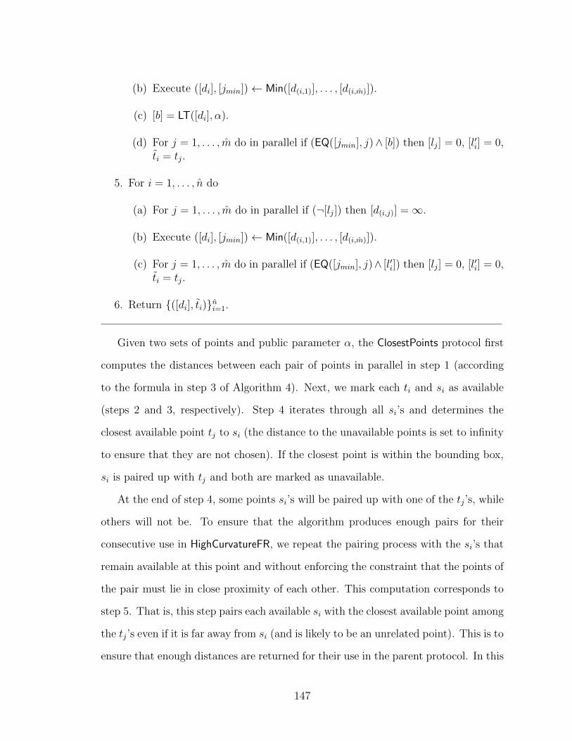
(b) Execute ([di

], [jmin

]) Min([d(i,1)

], . . . , [d(i,m)

]).

(c) [b] = LT([di

],↵).

(d) For j = 1, . . . , m do in parallel if (EQ([jmin

], j)^ [b]) then [lj

] = 0, [l0i

] = 0,ti

= tj

.

5. For i = 1, . . . , n do

(a) For j = 1, . . . , m do in parallel if (¬[lj

]) then [d(i,j)

] =1.

(b) Execute ([di

], [jmin

]) Min([d(i,1)

], . . . , [d(i,m)

]).

(c) For j = 1, . . . , m do in parallel if (EQ([jmin

], j)^ [l0i

]) then [lj

] = 0, [l0i

] = 0,ti

= tj

.

6. Return {([di

], ti

)}ni=1

.

Given two sets of points and public parameter ↵, the ClosestPoints protocol first

computes the distances between each pair of points in parallel in step 1 (according

to the formula in step 3 of Algorithm 4). Next, we mark each ti

and si

as available

(steps 2 and 3, respectively). Step 4 iterates through all si

’s and determines the

closest available point tj

to si

(the distance to the unavailable points is set to infinity

to ensure that they are not chosen). If the closest point is within the bounding box,

si

is paired up with tj

and both are marked as unavailable.

At the end of step 4, some points si

’s will be paired up with one of the tj

’s, while

others will not be. To ensure that the algorithm produces enough pairs for their

consecutive use in HighCurvatureFR, we repeat the pairing process with the si

’s that

remain available at this point and without enforcing the constraint that the points of

the pair must lie in close proximity of each other. This computation corresponds to

step 5. That is, this step pairs each available si

with the closest available point among

the tj

’s even if it is far away from si

(and is likely to be an unrelated point). This is to

ensure that enough distances are returned for their use in the parent protocol. In this

147

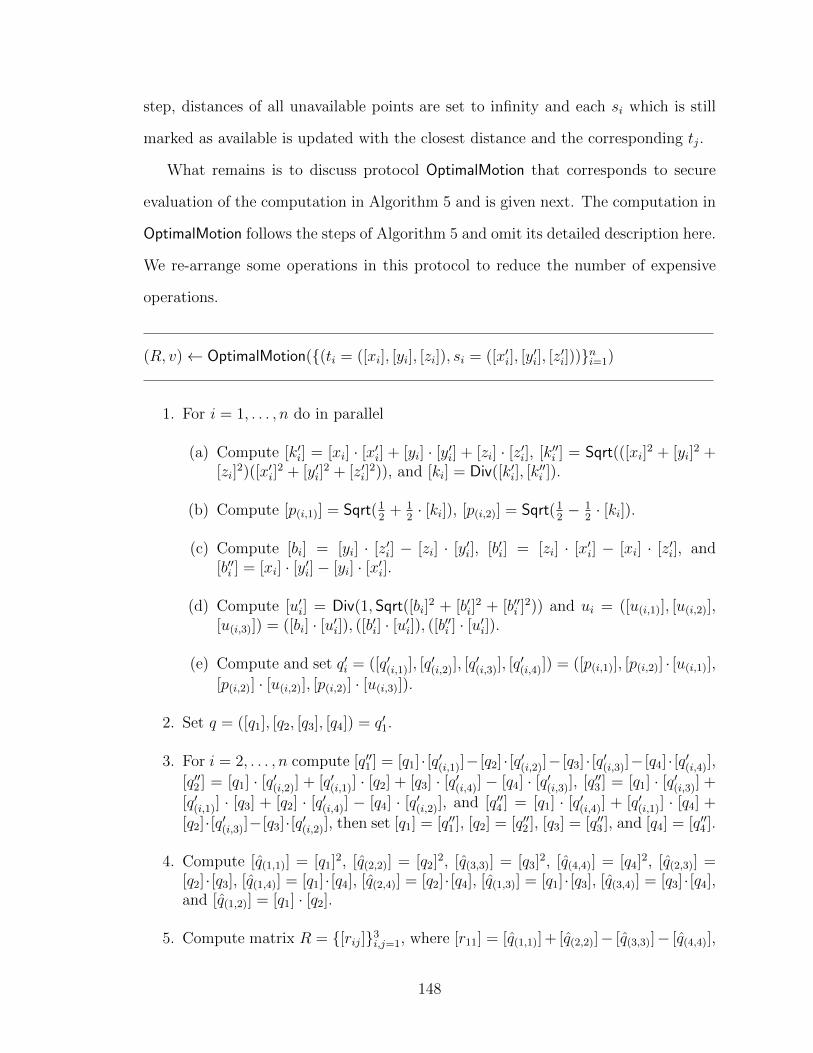
step, distances of all unavailable points are set to infinity and each si

which is still

marked as available is updated with the closest distance and the corresponding tj

.

What remains is to discuss protocol OptimalMotion that corresponds to secure

evaluation of the computation in Algorithm 5 and is given next. The computation in

OptimalMotion follows the steps of Algorithm 5 and omit its detailed description here.

We re-arrange some operations in this protocol to reduce the number of expensive

operations.

(R, v) OptimalMotion({(ti

= ([xi

], [yi

], [zi

]), si

= ([x0i

], [y0i

], [z0i

]))}ni=1

)

1. For i = 1, . . . , n do in parallel

(a) Compute [k0i

] = [xi

] · [x0i

] + [yi

] · [y0i

] + [zi

] · [z0i

], [k00i

] = Sqrt(([xi

]2 + [yi

]2 +[z

i

]2)([x0i

]2 + [y0i

]2 + [z0i

]2)), and [ki

] = Div([k0i

], [k00i

]).

(b) Compute [p(i,1)

] = Sqrt(12

+ 1

2

· [ki

]), [p(i,2)

] = Sqrt(12

� 1

2

· [ki

]).

(c) Compute [bi

] = [yi

] · [z0i

] � [zi

] · [y0i

], [b0i

] = [zi

] · [x0i

] � [xi

] · [z0i

], and[b00

i

] = [xi

] · [y0i

]� [yi

] · [x0i

].

(d) Compute [u0i

] = Div(1, Sqrt([bi

]2 + [b0i

]2 + [b00i

]2)) and ui

= ([u(i,1)

], [u(i,2)

],[u

(i,3)

]) = ([bi

] · [u0i

]), ([b0i

] · [u0i

]), ([b00i

] · [u0i

]).

(e) Compute and set q0i

= ([q0(i,1)

], [q0(i,2)

], [q0(i,3)

], [q0(i,4)

]) = ([p(i,1)

], [p(i,2)

] · [u(i,1)

],[p

(i,2)

] · [u(i,2)

], [p(i,2)

] · [u(i,3)

]).

2. Set q = ([q1

], [q2

, [q3

], [q4

]) = q01

.

3. For i = 2, . . . , n compute [q001

] = [q1

] · [q0(i,1)

]� [q2

] · [q0(i,2)

]� [q3

] · [q0(i,3)

]� [q4

] · [q0(i,4)

],[q00

2

] = [q1

] · [q0(i,2)

] + [q0(i,1)

] · [q2

] + [q3

] · [q0(i,4)

] � [q4

] · [q0(i,3)

], [q003

] = [q1

] · [q0(i,3)

] +[q0

(i,1)

] · [q3

] + [q2

] · [q0(i,4)

] � [q4

] · [q0(i,2)

], and [q004

] = [q1

] · [q0(i,4)

] + [q0(i,1)

] · [q4

] +[q

2

]·[q0(i,3)

]�[q3

]·[q0(i,2)

], then set [q1

] = [q001

], [q2

] = [q002

], [q3

] = [q003

], and [q4

] = [q004

].

4. Compute [q(1,1)

] = [q1

]2, [q(2,2)

] = [q2

]2, [q(3,3)

] = [q3

]2, [q(4,4)

] = [q4

]2, [q(2,3)

] =[q

2

]· [q3

], [q(1,4)

] = [q1

]· [q4

], [q(2,4)

] = [q2

]· [q4

], [q(1,3)

] = [q1

]· [q3

], [q(3,4)

] = [q3

]· [q4

],and [q

(1,2)

] = [q1

] · [q2

].

5. Compute matrix R = {[rij

]}3i,j=1

, where [r11

] = [q(1,1)

]+ [q(2,2)

]� [q(3,3)

]� [q(4,4)

],

148

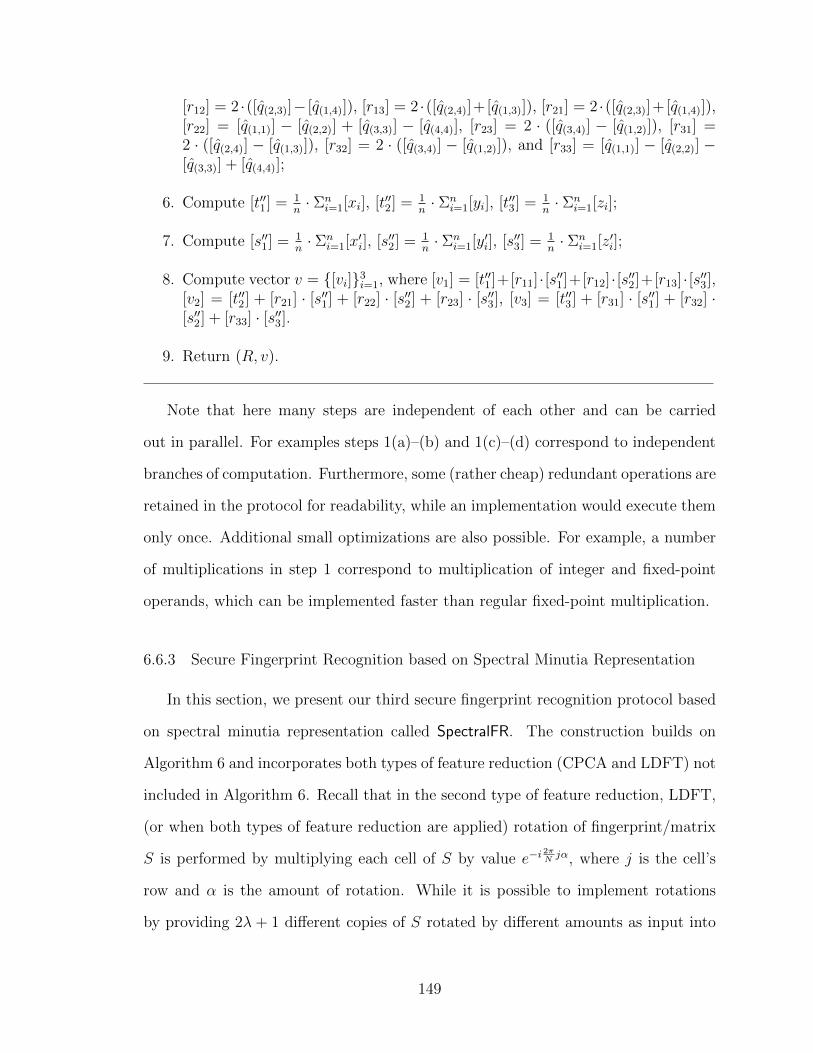
[r12

] = 2 ·([q(2,3)

]� [q(1,4)

]), [r13

] = 2 ·([q(2,4)

]+[q(1,3)

]), [r21

] = 2 ·([q(2,3)

]+[q(1,4)

]),[r

22

] = [q(1,1)

] � [q(2,2)

] + [q(3,3)

] � [q(4,4)

], [r23

] = 2 · ([q(3,4)

] � [q(1,2)

]), [r31

] =2 · ([q

(2,4)

] � [q(1,3)

]), [r32

] = 2 · ([q(3,4)

] � [q(1,2)

]), and [r33

] = [q(1,1)

] � [q(2,2)

] �[q

(3,3)

] + [q(4,4)

];

6. Compute [t001

] = 1

n

· ⌃n

i=1

[xi

], [t002

] = 1

n

· ⌃n

i=1

[yi

], [t003

] = 1

n

· ⌃n

i=1

[zi

];

7. Compute [s001

] = 1

n

· ⌃n

i=1

[x0i

], [s002

] = 1

n

· ⌃n

i=1

[y0i

], [s003

] = 1

n

· ⌃n

i=1

[z0i

];

8. Compute vector v = {[vi

]}3i=1

, where [v1

] = [t001

]+[r11

]·[s001

]+[r12

]·[s002

]+[r13

]·[s003

],[v

2

] = [t002

] + [r21

] · [s001

] + [r22

] · [s002

] + [r23

] · [s003

], [v3

] = [t003

] + [r31

] · [s001

] + [r32

] ·[s00

2

] + [r33

] · [s003

].

9. Return (R, v).

Note that here many steps are independent of each other and can be carried

out in parallel. For examples steps 1(a)–(b) and 1(c)–(d) correspond to independent

branches of computation. Furthermore, some (rather cheap) redundant operations are

retained in the protocol for readability, while an implementation would execute them

only once. Additional small optimizations are also possible. For example, a number

of multiplications in step 1 correspond to multiplication of integer and fixed-point

operands, which can be implemented faster than regular fixed-point multiplication.

6.6.3 Secure Fingerprint Recognition based on Spectral Minutia Representation

In this section, we present our third secure fingerprint recognition protocol based

on spectral minutia representation called SpectralFR. The construction builds on

Algorithm 6 and incorporates both types of feature reduction (CPCA and LDFT) not

included in Algorithm 6. Recall that in the second type of feature reduction, LDFT,

(or when both types of feature reduction are applied) rotation of fingerprint/matrix

S is performed by multiplying each cell of S by value e�i

2⇡N

j↵, where j is the cell’s

row and ↵ is the amount of rotation. While it is possible to implement rotations

by providing 2� + 1 di↵erent copies of S rotated by di↵erent amounts as input into

149

the protocol where � is the maximum amount of rotation, we perform any necessary

rotation inside the protocol to avoid the price of significantly increasing the input size.

We were also able to maintain performing only O(log �) score computations instead

of all 2� + 1 scores in our secure and oblivious protocol, which is an important

contribution of this work. Combined with avoiding to increase the input size to

have a linear dependency on �, this allows us to achieve low asymptotic complexity

and high e�ciency. Low asymptotic complexity is important because the size of

fingerprint representation is already large in this approach.

In what follows, we treat the case when � = 15 (with the total of 31 rotations

to be considered) as in the original algorithm [114], but it is not di�cult to gener-

alize the computation to any �. We apply our generalization and optimization of

Algorithm 6 described in Section 6.3.3 with 4 · 32 = 36 di↵erent rotations to cover

at least 31 necessary alignments. Note that this approach computes 8 similarity

scores instead of 9 in the original algorithm. We number all 36 rotations as ↵ =

�17, . . . , 18. The rotation constants e�i

2⇡N

j↵ = cos(�2⇡

N

j↵) + i sin(�2⇡

N

j↵) are fixed

and can be precomputed for each j = 1, . . . , N 0 and ↵ = �17, . . ., 18 by each party.

We denote these values by public matrix Z = {z↵,j

}18,N0

↵=�17,j=1

which each party stores

locally. Each z↵,j

is a tuple (z(1)↵,j

= cos(�2⇡

N

j↵), z(2)↵,j

= sin(�2⇡

N

j↵)), and Z is specified

as part of the input in SpectralFR.

To be able to compute only O(log �) scores in the protocol, we need to obliviously

determine the correct amount of rotation in steps 3 and 4 of Algorithm 6 without

revealing any information about k or k0 in those steps. We securely realize this

functionality by placing the values associated with each possible k or k0 in an array

and retrieving the right elements at a private index. In more detail, the protocol first

computes four scores that correspond to rotations by �13, �4, 3, and 12 positions

and computes the best among them (steps 3 and 4 below). Because the location of

the best score cannot be revealed, in the next step of the algorithm we put together

150

an array consisting of four vectors and one of them is privately selected using TLookup

(steps 4–5 of the protocol). The selected vector consists of 2N 0 values that allow us to

compute two new scores and the maximum score for the next iteration of algorithm.

We repeat the process of private retrieval of the necessary rotation coe�cients, this

time using an array consisting of twelve vectors. After computing two more scores

and determining the best score, the algorithm outputs the best score together with

the amount of rotation that resulted in that score.

The protocol SpectralFR is given next. Because SpectralFR corresponds to the

computation with both types of feature reduction, input matrices T and S are com-

posed of complex values. Thus, we represent each cell of T as a pair (ai,j

, bi,j

) with

the real and imaginary parts, respectively, and each cell of S as a pair (a0i,j

, b0i,j

). All

computations proceed over fixed-point values.

([Cmax

], [↵max

]) SpectralFR(T = {[ti,j

] = ([ai,j

], [bi,j

])}M0,N

0

i=1,j=1

, S = {[si,j

] = ([a0i,j

],

[b0i,j

])}M0,N

0

i=1,j=1

, Z = {zi,j

}18,N0

i=�17,j=1

,� = 15)

1. Set [Cmax

] = [0].

2. For i = 1, . . . ,M 0 and j = 1, . . . , N 0 do in parallel if (j 6= 1) then [xi,j

] =2([a

i,j

]·[a0i,j

]+[bi,j

]·[b0i,j

]), [yi,j

] = 2([a0i,j

]·[bi,j

]�[ai,j

]·[b0i,j

]), else [xi,j

] = [ai,j

]·[a0i,j

],[y

i,j

] = �[ai,j

] · [b0i,j

].

3. For k = 0, . . . , 3, do in parallel

(a) [C�13+9k

] = 0.

(b) For i = 1, . . . ,M 0 and j = 1, . . . , N 0 do [C�13+9k

] = [C�13+9k

] + z(1)�13+9k,j

·[x

i,j

] + z(2)�13+9k,j

· [yi,j

].

4. Compute the maximum as ([Cmax

], [↵max

]) Max([C�13

], [C�4

], [C5

], [C14

]).

5. For i = 0, . . . , 3 and j = 1, . . . , N 0 do in parallel z0i,j

= z�16+9i,j

and z0i,N

0+j

=z�10+9i,j

.

151

6. Let Z 0i

= (z0i,1

, . . ., z0i,2N

0) for i = 0, . . ., 3 and execute [Z 0max

] TLookup((Z 00

, . . .,Z 0

3

), [↵max

]); let [Z 0max

] = ([z1

], . . ., [z2N

0 ]).

7. For i = 1, . . . ,M 0 and j = 1, . . . , N 0 do [C↵

max

�3

] = [C↵

max

�3

] + [z(1)j

] · [xi,j

] +

[z(2)j

] · [yi,j

], [C↵

max

+3

] = [C↵

max

+3

] + [z(1)N

0+j

] · [xi,j

] + [z(2)N

0+j

] · [yi,j

].

8. Compute ([Cmax

], [↵max

]) Max([C↵

max

�3

], [Cmax

], [C↵

max

+3

]).

9. For i = 0, . . . , 11 and j = 1, . . . , N 0 do in parallel z0i,j

= z�17+3i,j

and z0i,N

0+j

=z�15+3i,j

.

10. Let Z 0i

= (z0i,1

, . . ., z0i,2N

0) for i = 0, . . ., 11 and execute [Z 0max

] TLookup((Z 00

, . . .,Z 0

11

), [↵max

]); let [Z 0max

] = ([z1

], . . ., [z2N

0 ]).

11. For i = 1, . . . ,M 0 and j = 1, . . . , N 0 do [C↵

max

�1

] = [C↵

max

�1

] + [z(1)j

] · [xi,j

] +

[z(2)j

] · [yi,j

], [C↵

max

+1

] = [C↵

max

+1

] + [z(1)N

0+j

] · [xi,j

] + [z(2)N

0+j

] · [yi,j

].

12. Compute ([Cmax

], [↵max

]) Max([C↵

max

�1

], [Cmax

], [C↵

max

+1

]).

13. Return [Cmax

] and [↵max

].

For e�ciency reasons, we perform all multiplications associated with the score

computation without any rotation in the beginning of the protocol (step 1). This

computation (i.e., multiplications of the real and imaginary components of each ti,j

and si,j

) is common to all score computations (see Equation 6.1) and is reused later

in the protocol. Then to compute a score between T and S rotated by ↵ positions,

the coe�cients from Z are multiplied to the computed products. In particular, the

computation takes form of {[z(1)↵,j

] · [xi,j

]}M0,N

0

i=1,j=1

and {[z(2)↵,j

] · [yi,j

]}M0,N

0

i=1,j=1

according to

Equation 6.1, which are added together to get the score. The rest of the protocol

proceeds as described above by using private table lookups twice. Note that the

result of each table lookup is an array as opposed to a single element. Also note

that the score computation uses public zi,j

’s in step 1(b), but the coe�cients become

private in steps 7 and 11 because they depend of private data. Finally, the factor 1

MN

2

present in Equation 6.1 is not included in the computation because it is public. The

computed score can be scaled down by this factor by an output recipient if necessary.

152

Recall that SpectralFR uses fixed-point arithmetic, but performance of some op-

erations can be optimized. For example, in the secret sharing setting, we can skip

truncation after each multiplication in step 7 or 11 and instead truncate the sum

after adding all products. In addition, we can restrict variables to shorter bitlength

representations when the range of values they store is known to be small. This is

relevant to multiplications in step 2 in the garbled circuit setting, where ti,j

and si,j

are known not to exceed N + 1 and can be represented using a short bitlength for

the integer part.

6.7 Performance Evaluation

In this section we evaluate performance of the spectral minutia representation

fingerprint recognition protocol SpectralFR to demonstrate that the proposed pro-

tocols are practical. We provide experimental results for both garbled circuit and

secret sharing settings. In the garbled circuit setting, our implementation uses the

JustGarble library [25, 26] for circuit garbling and garbled circuit evaluation which

we modified to support a half-gates optimization [116]. In the secret sharing setting,

we use PICCO [117] with three computational parties, which utilized linear threshold

secret sharing.

In our implementation, we assume that the inputs T and S are represented with

32-bit precision after the radix point. Our garbled circuit implementation maintains

56-bit fixed-point representation (24 and 32 bits before and after the radix point),

while in the secret sharing setting we let the numbers grow beyond the 56 bits to

avoid the cost of truncation, but perform truncation prior to returning the result.

We ran each experiment 10 times and report the mean value.

The results of SpectralFR performance evaluation can be found in Table 6.3 for the

three-party case and in Table 6.4 for the garbled circuit case. We report performance

for a range of parameters N 0 and M 0 that might be used in practice. All numbers

153

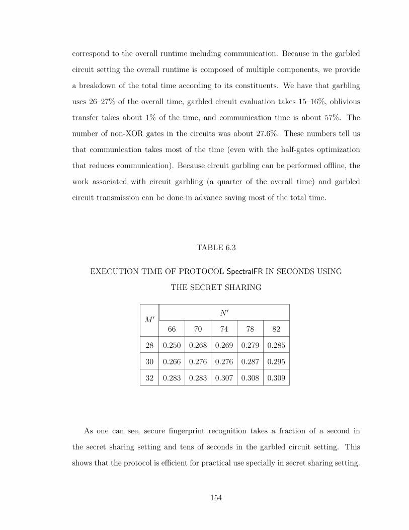
correspond to the overall runtime including communication. Because in the garbled

circuit setting the overall runtime is composed of multiple components, we provide

a breakdown of the total time according to its constituents. We have that garbling

uses 26–27% of the overall time, garbled circuit evaluation takes 15–16%, oblivious

transfer takes about 1% of the time, and communication time is about 57%. The

number of non-XOR gates in the circuits was about 27.6%. These numbers tell us

that communication takes most of the time (even with the half-gates optimization

that reduces communication). Because circuit garbling can be performed o✏ine, the

work associated with circuit garbling (a quarter of the overall time) and garbled

circuit transmission can be done in advance saving most of the total time.

TABLE 6.3

EXECUTION TIME OF PROTOCOL SpectralFR IN SECONDS USING

THE SECRET SHARING

M 0N 0

66 70 74 78 82

28 0.250 0.268 0.269 0.279 0.285

30 0.266 0.276 0.276 0.287 0.295

32 0.283 0.283 0.307 0.308 0.309

As one can see, secure fingerprint recognition takes a fraction of a second in

the secret sharing setting and tens of seconds in the garbled circuit setting. This

shows that the protocol is e�cient for practical use specially in secret sharing setting.

154

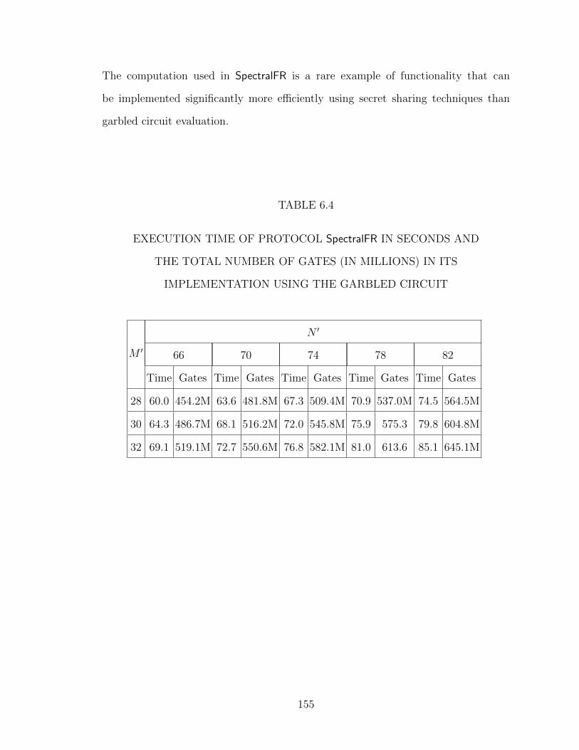
The computation used in SpectralFR is a rare example of functionality that can

be implemented significantly more e�ciently using secret sharing techniques than

garbled circuit evaluation.

TABLE 6.4

EXECUTION TIME OF PROTOCOL SpectralFR IN SECONDS AND

THE TOTAL NUMBER OF GATES (IN MILLIONS) IN ITS

IMPLEMENTATION USING THE GARBLED CIRCUIT

M 0

N 0

66 70 74 78 82

Time Gates Time Gates Time Gates Time Gates Time Gates

28 60.0 454.2M 63.6 481.8M 67.3 509.4M 70.9 537.0M 74.5 564.5M

30 64.3 486.7M 68.1 516.2M 72.0 545.8M 75.9 575.3 79.8 604.8M

32 69.1 519.1M 72.7 550.6M 76.8 582.1M 81.0 613.6 85.1 645.1M

155

CHAPTER 7

CONCLUSIONS AND FUTURE DIRECTIONS

In this chapter, we conclude our main contributions in this thesis in Section 7.1,

and then we focus on our future directions in Section 7.2.

7.1 Conclusions

In this thesis, we build general and time-e�cient privacy-preserving solutions

and protocols that can be used for di↵erent applications including voice recognition,

DNA computation, and fingerprint recognition where privacy of the data is one of

the main concerns. In the following, we conclude our main contributions for each

secure biometric modality.

7.1.1 Voice Recognition

We treat the problem of privacy-preserving Hidden Markov Models computation

which is commonly used for many applications including speaker recognition. We

develop provably secure techniques for HMM’s Viterbi and GMM computation using

floating-point arithmetic in both two-party setting using homomorphic encryption

and multi-party setting using secret sharing. These settings correspond to a variety

of real-life situations and the solutions were designed to minimize their overhead. A

significant part of this work is dedicated to new secure protocols for floating-point

operations in the malicious model in the two-party setting based on homomorphic en-

cryption. To the best of our knowledge, this is the first time such protocols are o↵ered

156

in the literature. We rigorously prove security of our protocols using simulation-based

proofs, which constitutes a distinct contribution of this work.

7.1.2 DNA Computation

We study server-aided secure garbled circuit computation in a number of security

settings. One of such security settings assumes that users A and B may act arbitrar-

ily and, in addition to requiring security in the presence of malicious users, we also

enforce that A and B enter their true inputs based on third party certification. We

are not aware of any prior work that combines input certification with general secure

multi-party computation based on Yao’s garbled circuits. We develop general solu-

tions in our server-aided framework. Despite their generality, they lead to e�cient

implementations of genetic tests. In particular, we design and implement genetic

paternity, compatibility, and common ancestry tests, all of which run in a matter of

seconds or less and favorably compare with the state of the art.

7.1.3 Fingerprint Recognition

We design three secure and e�cient protocols for fingerprint alignment and match-

ing for garbled circuit and secret sharing settings. They are based on popular algo-

rithms in the computer vision literature and employ new non-trivial techniques. The

constructions are presented in the semi-honest setting and known results can be ap-

plied to strengthen the security to sustain malicious actors. We believe that this is

the first work that treats the problem of secure fingerprint alignment. We also design

secure constructions for fundamental numeric and set operations. We present novel

secure protocols for sine, cosine, arctangent, and square root for fixed-point numbers,

as well as a novel secure and data-oblivious protocol for selection of the fth smallest

element of a set (for any type of data). The techniques are applicable to both garbled

circuit and secret sharing settings.

157

7.2 Future Plan

It is our goal to continue expanding upon our existing research as well as to

incorporate and design new techniques enhancing the research areas of of security,

privacy, and applied cryptography. This plan also includes exploring other research

directions within information security and how methods within this current field

could benefit biometric challenges. In particular, we are interested in working on the

following topics:

7.2.1 E�cient Input Certification Protocols

In the current literature, the strongest security settings are defined in the pres-

ence of malicious parties, and usually, the correctness of the entered inputs is not

considered in the computations. As a result, a malicious party can modify her in-

puts to learn more information about the other party’s inputs. Therefore, there is a

high-priority need for a stronger security model to guarantee that all parties provide

authorized information in the computations. For this purpose, we plan to provide ef-

ficient certified input solutions for di↵erent computational settings that could benefit

a variety of applications. In [118], you can find our progress in designing a certified

input solution based on garbled circuit evaluation.

7.2.2 Secure Protocols in the Presence of a Covert Adversary

There is another adversarial model known as “covert adversarial model”. Covert

adversaries may deviate arbitrarily from the protocol specification in an attempt to

cheat, but they do not wish to be caught. This unique property of the covert user

makes it more practical in real-world situations because it may be the case that the

risk of being caught is evaluated against the benefits of cheating. Therefore, we are

interested in building e�cient and secure protocols in this adversarial model and

in applying them to di↵erent applications including secure biometric computations.

158

These protocols will be secure enough, and well-suited to the downstream applica-

tions. In addition, these protocols designed under the covert adversarial assumption

will computationally outperform those under the malicious adversarial assumption.

7.2.3 Data Mining Computations on Large-Scale Data Sets

Classification, clustering, and frequent pattern mining are common practices for

knowledge discovery on large-scale data sets. In many cases the data is not public

and it is sensitive; therefore, protection of the data is a major requirement. In data

mining on large-scale data sets, utility and privacy of data are two main goals for

which accomplishing one may lead to an undesired impact on the other. Nowadays,

there is a big challenge and urgent need to achieve both practicality on downstream

applications and privacy preservation of sensitive data in data mining and knowledge

discovery solutions. As a future direction, we plan to design a set of practical in terms

of e�ciency and general-form secure solutions to carry out classification, clustering,

or frequent pattern mining algorithms to address the research challenge in this area.

159

BIBLIOGRAPHY

1. 23andMe – Genetic Testing for Ancestry; DNA Test. http://www.23andme.com.

2. Genealogy, Family Trees & Family History Records at Ancestry.com.http://www.ancestry.com.

3. GenePartner.com – DNA matching: Love is no coincidence.http://www.genepartner.com.

4. GMP – The GNU multiple precision arithmetic library. http://www.gmplib.org.

5. NIST special database 4. https://www.nist.gov/srd/nist-special-database-4.

6. OpenSSL: The open source toolkit for SSL/TLS. http://www.openssl.org.

7. Fingerprint minutiae viewer (FpMV). https://www.nist.gov/services-resources/software/fingerprint-minutiae-viewer-fpmv.

8. Secure supply chain management (SecureSCM) project deliverable: D9.2 secu-rity analysis, July 2009.

9. M. Aliasgari. Secure computation and outsourcing of biometric data. Universityof Notre Dame, 2013.

10. M. Aliasgari and M. Blanton. Secure computation of hidden markov models. InInternational Conference on Security and Cryptography, 2013.

11. M. Aliasgari, M. Blanton, Y. Zhang, and A. Steele. Secure computation onfloating point numbers. In Network and Distributed Security Symposium, 2013.

12. M. Aliasgari, M. Blanton, and F. Bayatbabolghani. Secure computation ofhidden markov models and secure floating-point arithmetic in the maliciousmodel. International Journal of Information Security, to appear.

13. G. Asharov, Y. Lindell, and T. Rabin. Perfectly-secure multiplication for anyt < n/3. In Cryptology Conference (CRYPTO), pages 240–258, 2011.

14. G. Asharov, Y. Lindell, T. Schneider, and M. Zohner. More e�cient oblivioustransfer and extensions for faster secure computation. In ACM Conference onComputer and Communications Security, pages 535–548, 2013.

160

15. M. Atallah, M. Bykova, J. Li, K. Frikken, and M. Topkara. Private collaborativeforecasting and benchmarking. In ACM Workshop on Privacy in the ElectronicSociety, pages 103–114, 2004.

16. E. Ayday, J. L. Raisaro, and J.-P. Hubaux. Privacy-enhancing technology formedical tests using genomic data. Technical Report EPFL-REPORT-182897,EPFL, 2012.

17. E. Ayday, J. L. Raisaro, and J. Hubaux. Personal use of genomic data: Privacyvs. storage cost. In IEEE Global Communications Conference, pages 2723–2729,2013.

18. E. Ayday, J. L. Raisaro, J.-P. Hubaux, and J. Rougemont. Protecting andevaluating genomic privacy in medical tests and personalized medicine. In ACMWorkshop on Privacy in the Electronic Society, pages 95–106, 2013.

19. E. Ayday, J. L. Raisaro, P. McLaren, J. Fellay, and J.-P. Hubaux. Privacy-preserving computation of disease risk by using genomic, clinical, and environ-mental data. In USENIX Workshop on Health Information Technologies, 2013.

20. P. Baldi, R. Baronio, E. De Cristofaro, P. Gasti, and G. Tsudik. CounteringGATTACA: E�cient and secure testing of fully-sequenced human genomes. InACM Conference on Computer and Communications Security, pages 691–702,2011.

21. P. Bansal, A. Kant, S. Kumar, A. Sharda, and S. Gupta. Improved hybrid modelof hmm/gmm for speech recognition. In Book 5 Intelligent Technologies andApplications. Institute of Information Theories and Applications FOI ITHEA,2008.

22. M. Barni, T. Bianchi, D. Catalano, M. Di Raimondo, R. Labati, P. Failla,D. Fiore, R. Lazzeretti, V. Piuri, F. Scotti, and A. Piva. Privacy-preservingFingerCode authentication. In ACM Workshop on Multimedia and Security,pages 231–240, 2010.

23. K. Batcher. Sorting networks and their applications. In AFIPS Spring JointComputer Conference, pages 307–314, 1968.

24. F. Bayatbabolghani, M. Blanton, M. Aliasgari, and M. Goodrich. Secure fin-gerprint alignment and matching protocols. arXiv Report 1702.03379, 2017.

25. M. Bellare, V. T. Hoang, S. Keelveedhi, and P. Rogaway. The JustGarblelibrary. http://cseweb.ucsd.edu/groups/justgarble/.

26. M. Bellare, V. Hoang, S. Keelveedhi, and P. Rogaway. E�cient garbling froma fixed-key blockcipher. In IEEE Symposium of Security and Privacy, pages478–492, 2013.

161

27. P. Besl and N. McKay. Method for registration of 3-D shapes. IEEE Transac-tions on Pattern Analysis and Machine Intelligence, 14(2):239–256, 1992.

28. M. Blanton. Empirical evaluation of secure two-party computation models.Technical Report TR 2005-58, CERIAS, Purdue University, 2005.

29. M. Blanton. Achieving full security in privacy-preserving data mining. In IEEEInternational Conference on Information Privacy, Security, Risk and Trust,pages 925–934, 2011.

30. M. Blanton and E. Aguiar. Private and oblivious set and multiset operations.International Journal of Information Security, 15(5):493–518, Oct. 2016.

31. M. Blanton and F. Bayatbabolghani. E�cient server-aided secure two-partyfunction evaluation with applications to genomic computation. Proceedings onPrivacy Enhancing Technologies, 4:144–164, 2016.

32. M. Blanton and F. Bayatbabolghani. An approach to improving security ande�ciency of private genomic computation using server aid. IEEE Security andPrivacy Magazine, 2017.

33. M. Blanton and P. Gasti. Secure and e�cient protocols for iris and fingerprintidentification. In European Symposium on Research in Computer Security, pages190–209, 2011.

34. M. Blanton and P. Gasti. Secure and e�cient iris and fingerprint identifica-tion. In D. Ngo, A. Teoh, and J. Hu, editors, Biometric Security, chapter 9.Cambridge Scholars Publishing, 2015.

35. M. Blanton and S. Saraph. Oblivious maximum bipartite matching size algo-rithm with applications to secure fingerprint identification. In European Sym-posium on Research in Computer Security, pages 384–406, 2015.

36. F. Bruekers, S. Katzenbeisser, K. Kursawe, and P. Tuyls. Privacy-preservingmatching of DNA profiles. IACR Cryptology ePrint Archive Report 2008/203,2008.

37. J. Camenisch and A. Lysyanskaya. A signature scheme with e�cient protocols.In Conference on Security and Cryptography for Networks, pages 268–289, 2002.

38. J. Camenisch and A. Lysyanskaya. Signature schemes and anonymous creden-tials from bilinear maps. In Cryptology Conference (CRYPTO), pages 56–72,2004.

39. J. Camenisch and M. Michels. Separability and e�ciency for generic groupsignature schemes. In Cryptology Conference (CRYPTO), 1999.

40. J. Camenisch and M. Stadler. E�cient group signature schemes for large groups.In Cryptology Conference (CRYPTO), 1997.

162

41. J. Camenisch and M. Stadler. Proof systems for general statements about dis-crete logarithms. Technical report, Institute for Theoretical Computer Science,ETH Zurich, 1997.

42. J. Camenisch and G. Zaverucha. Private intersection of certified sets. In Finan-cial Cryptography and Data Security, pages 108–127, 2009.

43. J. Camenisch, D. Sommer, and R. Zimmermann. A general certification frame-work with applications to privacy-enhancing certificate infrastructures. In Se-curity and Privacy in Dynamic Environments, pages 25–37, 2006.

44. R. Canetti. Security and composition of multiparty cryptographic protocols.Journal of Cryptology, 13(1):143–202, 2000.

45. O. Catrina and S. de Hoogh. Improved primitives for secure multiparty integercomputation. In Security and Cryptography for Networks, pages 182–199, 2010.

46. O. Catrina and A. Saxena. Secure computation with fixed-point numbers. InFinancial Cryptography and Data Security, pages 35–50, 2010.

47. CertiVox. Multiprecision integer and rational arithmetic cryptographic library(MIRACL). http://www.certivox.com/miracl/.

48. D. Chetverikov, D. Svirko, D. Stepanov, and P. Krsek. The trimmed iterativeclosest point algorithm. In International Conference on Pattern Recognition,pages 545–548, 2002.

49. R. Cleve. Limits on the security of coin flips when half the processors are faulty.In ACM Symposium on Theory of Computing, pages 573–588, 1986.

50. R. Cramer, I. Damgard, and J. Nielsen. Multiparty computation from thresholdhomomorphic encryption. In International Conference on the Theory and Ap-plications of Cryptographic Techniques (EUROCRYPT), pages 280–289, 2001.

51. I. Damgaard and E. Fujisaki. A statistically-hiding integer commitment schemebased on groups with hidden order. In International Conference on the Theoryand Application of Cryptology and Information Security (ASIACRYPT), pages125–142, 2002.

52. I. Damgard and M. Jurik. A generalisation, a simplification and some appli-cations of Paillier’s probabilistic public-key system. In International Workshopon Practice and Theory in Public Key Cryptography, pages 119–136, 2001.

53. I. Damgard and J. Nielsen. Universally composable e�cient multiparty com-putation from threshold homomorphic encryption. In Cryptology Conference(CRYPTO), pages 247–264, 2003.

163

54. I. Damgard, Y. Ishai, and M. Krøigaard. Perfectly secure multiparty com-putation and the computational overhead of cryptography. In InternationalConference on the Theory and Applications of Cryptographic Techniques (EU-ROCRYPT), pages 445–465, 2010.

55. E. De Cristofaro and G. Tsudik. Practical private set intersection protocols withlinear complexity. In Financial Cryptography and Data Security, pages 143–159,2010.

56. E. De Cristofaro, S. Faber, P. Gasti, and G. Tsudik. GenoDroid: Are privacy-preserving genomic tests ready for prime time? In ACM Workshop on Privacyin the Electronic Society, pages 97–107, 2012.

57. E. De Cristofaro, S. Faber, and G. Tsudik. Secure genomic testing with size-and position-hiding private substring matching. In ACM Workshop on Privacyin the Electronic Society, pages 107–118, 2013.

58. U. Feige, J. Kilian, and M. Naor. A minimal model for secure computation. InACM Symposium on Theory of Computing, pages 554–563, 1994.

59. A. Fiat and A. Shamir. How to prove yourself: Practical solutions to iden-tification and signature scheme. In Cryptology Conference (CRYPTO), pages186–194, 1986.

60. M. Franz. Secure Computations on Non-Integer Values. PhD thesis, TU Darm-stadt, 2011.

61. M. Franz, B. Deiseroth, K. Hamacher, S. Jha, S. Katzenbeisser, and H. Schroder.Towards secure bioinformatics services (short paper). In Financial Cryptographyand Data Security, pages 276–283. Springer, 2012.

62. E. Fujisaki and T. Okamoto. Statistical zero knowledge protocols to provemodular polynomial relations. In Cryptology Conference (CRYPTO), pages 16–30, 1997.

63. R. Gamboa and J. Cowles. Formal verification of medina’s sequence of polyno-mials for approximating arctangent. arXiv preprint arXiv:1406.1561, 2014.

64. R. Gennaro, M. Rabin, and T. Rabin. Simplified VSS and fast-track multipartycomputations with applications to threshold cryptography. In ACM Symposiumon Principles of Distributed Computing, pages 101–111, 1998.

65. O. Goldreich. Foundations of Cryptography: Volume 2, Basic Applications.Cambridge University Press, 2004.

66. M. Golestanian, H. Nikoo, and J. Sadri. Intron profile analysis approach for exondetection in dna sequences using spectral analysis. Journal of Bioinformaticsand Intelligent Control, 3(2):140–142, 2014.

164

67. M. Goodrich. Data-oblivious external-memory algorithms for the compaction,selection, and sorting of outsourced data. In ACM Symposium on Parallelismin Algorithms and Architectures, pages 379–388, 2011.

68. J. Hart, E. Cheney, C. Lawson, H. Maehly, C. Mesztenyi, J. Rice, H. Thacher,and C. Witzgall. Computer approximations. John Wiley & Sons, Inc., 1968.

69. D. He, N. Furlotte, F. Hormozdiari, J. Joo, A. Wadia, R. Ostrovsky, A. Sa-hai, and E. Eskin. Identifying genetic relatives without compromising privacy.Genome Research, 24:664–672, 2014.

70. W. Henecka, K. Stefan, A. R. Sadeghi, T. Schneider, and I. Wehrenberg. Tasty:Tool for automating secure two-party computations. In ACM Conference onComputer and Communications Security, pages 451–462. ACM, 2010.

71. A. Herzberg and H. Shulman. Oblivious and fair server-aided two-party com-putation. In International Conference on Availability, Reliability and Security,pages 75–84, 2012.

72. F. Hormozdiari, J. Joo, A. Wadia, F. Guan, R. Ostrovsky, A. Sahai, and E. Es-kin. Privacy preserving protocol for detecting genetic relatives using rare vari-ants. Bioinformatics, pages 204–2011, 2014.

73. B. Horn. Closed-form solution of absute orientation using unit quaternions.Journal of the Optical Society of America A, 4(4):629–642, 1987.

74. Y. Huang, L. Malka, D. Evans, and J. Katz. E�cient privacy-preserving bio-metric identification. In Network and Distributed System Security Symposium,2011.

75. Y. Huang, J. Katz, and D. Evans. Quid-pro-quo-tocols: Strengthening semi-honest protocols with dual execution. In IEEE Symposium of Security andPrivacy, 2012.

76. Y. Ishai, J. Kilian, K. Nissim, and E. Petrank. Extending oblivious transferse�ciently. In Cryptology Conference (CRYPTO), pages 145–161, 2003.

77. S. Jarecki and V. Shmatikov. E�cient two-party secure computation on com-mitted inputs. In International Conference on the Theory and Applications ofCryptographic Techniques (EUROCRYPT), pages 97–114, 2007.

78. S. Kamara, P. Mohassel, and M. Raykova. Outsourcing multi-party computa-tion. IACR Cryptology ePrint Archive Report 2011/272, 2011.

79. S. Kamara, P. Mohassel, and B. Riva. Salus: A system for server-aided securefunction evaluation. In ACM Conference on Computer and CommunicationsSecurity, pages 797–808, 2012.

165

80. A. Karatsuba and Y. Ofman. Multiplication of many-digital numbers by auto-matic computers. Doklady Akademii Nauk SSSR, 145:293–294, 1962.

81. J. Katz and L. Malka. Secure text processing with applications to private DNAmatching. In ACM Conference on Computer and Communications Security,pages 485–492, 2010.

82. F. Kerschbaum, M. Atallah, D. M’Raıhi, and J. Rice. Private fingerprint ver-ification without local storage. In International Conference on Biometric Au-thentication, pages 387–394, 2004.

83. M. Kiraz, T. Schoenmakers, and J. Villegas. E�cient committed oblivioustransfer of bit strings. In Information Security Conference, pages 130–144, 2007.

84. V. Kolesnikov and T. Schneider. Improved garbled circuit: Free XOR gatesand applications. In International Colloquium on Automata, Languages andProgramming, pages 486–498, 2008.

85. V. Kolesnikov, A. R. Sadeghi, and T. Schneider. Improved garbled circuit build-ing blocks and applications to auctions and computing minima. In Cryptologyand Network Security, pages 1–20. Springer, 2009.

86. V. Kolesnikov, R. Kumaresan, and A. Shikfa. E�cient verification of inputconsistency in server-assisted secure function evaluation. In Cryptology andNetwork Security, pages 201–217, 2012.

87. B. Kreuter, A. Shelat, and C. Shen. Billion-gate secure computation with ma-licious adversaries. In USENIX Security Symposium, 2012.

88. M. Liedel. Secure distributed computation of the square root and applications.In Information Security Practice and Experience, pages 277–288. Springer, 2012.

89. Y. Lindell. Fast cut-and-choose based protocols for malicious and covert adver-saries. In Cryptology Conference (CRYPTO), 2013.

90. Y. Lindell and B. Pinkas. A proof of security of Yao’s protocol for two-partycomputation. Journal of Cryptology, 22(2):161–188, 2009.

91. Y. Lindell and B. Pinkas. Secure two-party computation via cut-and-chooseoblivious transfer. Journal of Cryptology, 25(4):680–722, 2012.

92. D. Maltoni, D. Maio, A. K. Jain, and S. Prabhakar. Handbook of FingerprintRecognition. New York Springer-Verlag, 2003.

93. T. Matsui and S. Furui. Speaker adaptation of tied-mixture-based phonememodels for text-prompted speaker recognition. In IEEE International Confer-ence on Acoustics, Speech, and Signal Processing, volume 1, pages 125–128,1994.

166

94. H. A. Medina. A sequence of polynomials for approximating arctangent. TheAmerican Mathematical Monthly, 113(2):156–161, 2006.

95. P. Mohassel and M. Franklin. E�ciency tradeo↵s for malicious two-party com-putation. In Public Key Cryptography, pages 458–73, 2006.

96. P. Mohassel and B. Riva. Garbled circuits checking garbled circuits: More e�-cient and secure two-party computation. In Cryptology Conference (CRYPTO),pages 36–53, 2013.

97. P. Mohassel, M. Rosulek, and Y. Zhang. Fast and secure three-party compu-tation: The garbled circuit approach. In ACM Conference on Computer andCommunications Security, pages 591–602, 2015.

98. K. Nandakumar, A. K. Jain, and S. Pankanti. Fingerprint-based fuzzy vault:Implementation and performance. IEEE Transactions on Information Forensicsand Security, 2(4):744–757, 2007.

99. M. Naor and B. Pinkas. E�cient oblivious transfer protocols. In ACM-SIAMSymposium on Discrete Algorithms, pages 448–457, 2001.

100. H. Nguyen and M. Roughan. Multi-observer privacy-preserving hidden markovmodels. In Network Operations and Management Symposium, pages 514–517,2012.

101. H. Nguyen and M. Roughan. On the identifiability of multi-observer hiddenmarkov models. In International Conference on Acoustics, Speech and SignalProcessing, pages 1873–1876, 2012.

102. P. Paillier. Public-key cryptosystems based on composite degree residuosityclasses. In International Conference on the Theory and Applications of Crypto-graphic Techniques (EUROCRYPT), pages 223–238, 1999.

103. M. Pathak and B. Raj. Privacy preserving speaker verification using adaptedGMMs. In Interspeech, pages 2405–2408, 2011.

104. M. Pathak, S. Rane, W. Sun, and B. Raj. Privacy preserving probabilisticinference with hidden Markov models. In International Conference on Acoustics,Speech and Signal Processing, pages 5868–5871, 2011.

105. M. Pathak, J. Portelo, B. Raj, and I. Trancoso. Privacy-preserving speakerauthentication. Information Security Conference (ISC), pages 1–22, 2012.

106. M. Pathak, B. Raj, S. Rane, and P. Saragdis. Privacy-preserving speech pro-cessing: cryptographic and string-matching frameworks show promise. IEEESignal Processing Magazine, 30(2):62–74, 2013.

107. H. Polat, W. Du, S. Renckes, and Y. Oysal. Private predictions on hiddenMarkov models. Artificial Intelligence Review, 34(1):53–72, 2010.

167

108. S. Shahandashti, R. Safavi-Naini, and P. Ogunbona. Private fingerprint match-ing. In Australasian Conference on Information Security and Privacy, pages426–433, 2012.

109. A. Shahbazi, F. Bayatbabolghani, and M. Blanton. Private computation withgenomic data for genome-wide association and linkage studies. In InternationalWorkshop on Genomic Privacy and Security, 2016.

110. A. Shamir. How to share a secret. Communications of the ACM, 22(11):612–613,1979.

111. M. Shashanka. A privacy preserving framework for Gaussian mixture models.In IEEE International Conference on Data Mining Workshops, pages 499–506.IEEE, 2010.

112. A. Shelat and C. h. Shen. Two-output secure computation with malicious ad-versaries. In International Conference on the Theory and Applications of Cryp-tographic Techniques (EUROCRYPT), 2011.

113. P. Smaragdis and M. Shashanka. A framework for secure speech recognition.IEEE Transactions on Audio, Speech, and Language Processing, 15(4):1404–1413, 2007.

114. H. Xu, R. Veldhuis, A. Bazen, T. Kevenaar, T. Akkermans, and B. Gokberk.Fingerprint verification using spectral minutiae representations. IEEE Trans-actions on Information Forensics and Security, 4(3):397–409, 2009.

115. H. Xu, R. Veldhuis, T. Kevenaar, and T. Akkermans. A fast minutiae-basedfingerprint recognition system. IEEE Systems Journal, 3(4):418–427, 2009.

116. S. Zahur, M. Rosulek, and D. Evans. Two halves make a whole: Reducing datatransfer in garbled circuits using half gates. In International Conference on theTheory and Applications of Cryptographic Techniques (EUROCRYPT), pages220–250, 2015.

117. Y. Zhang, A. Steele, and M. Blanton. Picco: A general-purpose compiler forprivate distributed computation. In ACM Conference on Computer and Com-munications Security, pages 813–826, 2013.

118. Y. Zhang, M. Blanton, and F. Bayatbabolghani. Enforcing input correctnessvia certification in garbled circuit evaluation. Cryptology ePrint Archive Report2017/569, 2017.

This document was prepared & typeset with pdfL

AT

E

X, and formatted with

nddiss2" classfile (v3.2013[2013/04/16]) provided by Sameer Vijay and updated

by Megan Patnott.

168

SECURE BIOMETRIC COMPUTATION AND …fbayatba/Publications/Thesis-phd.pdfSECURE BIOMETRIC COMPUTATION...

Documents

Transcript of SECURE BIOMETRIC COMPUTATION AND …fbayatba/Publications/Thesis-phd.pdfSECURE BIOMETRIC COMPUTATION...