Secular Trends and Technological Progress

Robin Dottling1 and Enrico Perotti ∗2

1University of Amsterdam and Tinbergen Institute2University of Amsterdam, CEPR and Tinbergen Institute

October 2017

Abstract

Technological progress enhancing the productivity of skills and intangible capital can

account for long term financial trends since 1980. As creating intangibles requires commit-

ment of human capital rather than physical investment, firms need less external finance.

As intangible capital become more productive, innovators gain a rising income share. The

general equilibrium effect is a falling credit demand, consistent with falling trends in both

tangible investment and interest rates. Another effect is a boost to asset valuation and

rising credit demand to fund house purchases. The combination of rising house prices and

increasing inequality raises household leverage and default risk.

While demographics, capital flows and trade also contribute to a savings glut and

changes in factor productivity, only a strong technological shift towards intangibles can

account for all major trends, including income polarization and a reallocation of credit

from productive to asset financing.

Keywords. Intangible capital, skill-biased technological change, mortgage credit, human

capital, excess savings, house prices

JEL classifications. D33, E22, G32, J24

∗We are very grateful to Bjorn Brugemann for many helpful discussions, to Paul Romer, Viral Acharya,Dimitris Papanikolaou, Gregory Thwaites and Eric Bartelsman for their valuable comments, Kasper Goosenfor research assistance, and seminar participants at Columbia University, NYU, LSE, CREI-UPF, theUniversity of Amsterdam, Tinbergen Institute, European Central Bank, Free University Amsterdam, Bankof Finland, DNB and Bank of England. Earlier versions were circulated under the title ”TechnologicalChange and the Evolution of Finance”.

1

1. Introduction

This paper proposes a growth model describing the general equilibrium impact of technologi-

cal change on long term financial trends such as interest rates, asset prices and the allocation

of credit. It suggests that the transition to a knowledge-based economy and the associated

shift from physical to intangible capital is a primary cause for the rising excess savings over

productive investment in advanced economies, presented in the “secular stagnation” hypoth-

esis (Summers, 2014; Eichengreen, 2015). Falling interest rates and rising long term asset

values can be interpreted as a direct consequence of this gradual process. Critically, the

approach also allows to interpret the growing share of income gained by innovators, the pro-

gressive reallocation of credit from productive to asset financing uses (primarily for housing)

and the rise in household leverage.

Information technology is widely recognized as a main cause for the rising productivity of

high-skill workers, leading to a steady increase in wage inequality and skill premia (e.g. see

Autor et al., 1998, 2003). On the capital front it has led to an increasing ratio of intangible

to tangible investment (Corrado and Hulten, 2010a), as figure 1 documents.

Our focus is to understand the consequences of this transition. A key economic insight

is that intangible capital is mostly the result of human capital investment which, unlike

tangible capital, cannot be purchased by firms.1 The transition to intangible investment thus

requires less external funding, as compensation to motivate and retain creative employees

takes place over time as output is realized. Indeed, the evidence is that firms that invest more

in intangibles have lower or even negative net leverage. This shift is often explained by poor

pledgeability of intangible assets (Bates et al., 2009; Falato et al., 2013).

This paper suggests that a declining corporate demand appears a more likely explanation

than tighter financial constraints. More generally, it proposes that technological progress

underlying the evolution of corporate assets offers an interpretation for major financial and

economic trends since 1980, such as secular stagnation, credit reallocation and rising asset

1Hart and Moore (1994) offer the classic analysis on the inalienability of human capital.

2

Figure 1: Evolution of the intangible capital ratio since 1980.

The intangibles ratio is defined as the ratio of intangible capital to total capital. The Compustat

ratio is computed using the measure of intangible capital of Peters and Taylor (2017). In the

BEA data the intangibles ratio is defined as intellectual property products (IPP) over total fixed

assets in the NIPA tables.

valuations.

We consider an overlapping generation (OLG) growth model with several productive factors.

In its general formulation of production, physical capital is complementary with manual labor

while intangible capital is complementary with high-skill labor. As physical capital is fully

pledgeable, firms can scale up investment to the point where its marginal productivity equals

the cost of borrowing. In contrast, intangible capital is developed by innovative employees,

who capture part of its returns. The OLG setup describes life-cycle savings behavior, where

land serves as both durable consumption good and as a store of value. Young households save

by investing in financial claims and housing, and consume when old.

Our benchmark view of technological change is a steady increase in the relative productivity

of intangible capital and skilled labor. Over time intangibles become more productive, so

intangible investment rises relative to phsyical investment. This has two effects. Firms expand

3

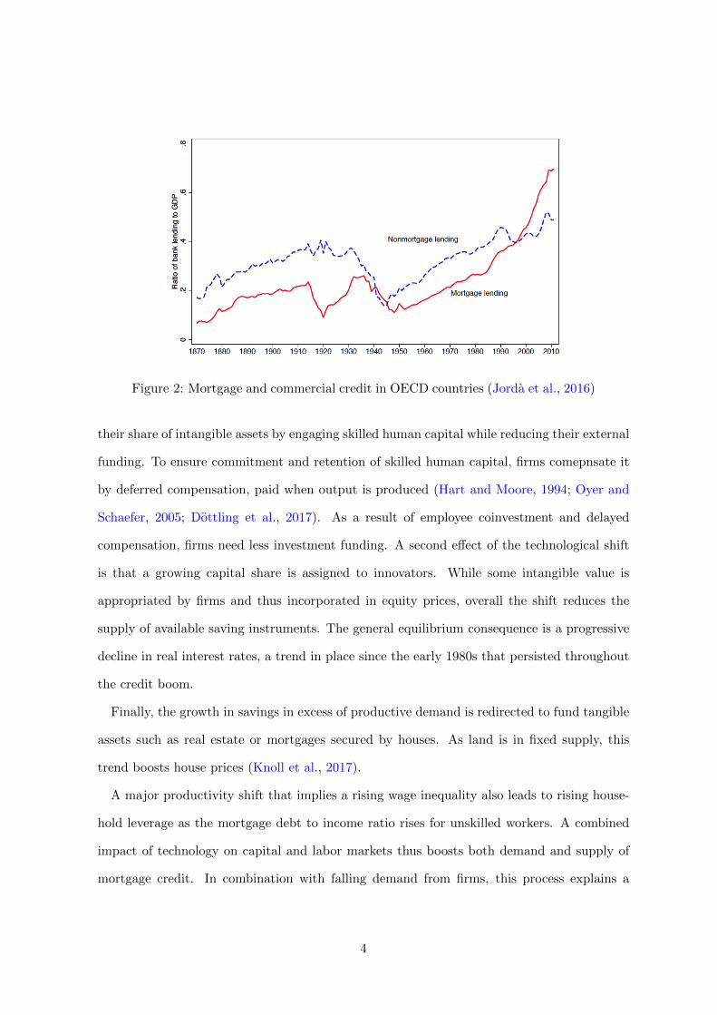
Figure 2: Mortgage and commercial credit in OECD countries (Jorda et al., 2016)

their share of intangible assets by engaging skilled human capital while reducing their external

funding. To ensure commitment and retention of skilled human capital, firms comepnsate it

by deferred compensation, paid when output is produced (Hart and Moore, 1994; Oyer and

Schaefer, 2005; Dottling et al., 2017). As a result of employee coinvestment and delayed

compensation, firms need less investment funding. A second effect of the technological shift

is that a growing capital share is assigned to innovators. While some intangible value is

appropriated by firms and thus incorporated in equity prices, overall the shift reduces the

supply of available saving instruments. The general equilibrium consequence is a progressive

decline in real interest rates, a trend in place since the early 1980s that persisted throughout

the credit boom.

Finally, the growth in savings in excess of productive demand is redirected to fund tangible

assets such as real estate or mortgages secured by houses. As land is in fixed supply, this

trend boosts house prices (Knoll et al., 2017).

A major productivity shift that implies a rising wage inequality also leads to rising house-

hold leverage as the mortgage debt to income ratio rises for unskilled workers. A combined

impact of technology on capital and labor markets thus boosts both demand and supply of

mortgage credit. In combination with falling demand from firms, this process explains a

4

declining stock of productive credit relative to mortgage credit across all OECD countries

(Jorda et al., 2016, see figure 2).

We compare this hypothesis with alternative views of the growth process consistent with

secular stagnation and other historical trends. Other formulations of technological change

include a rise in capital productivity, an increasing rate of innovation, more productive in-

tangibles and a higher level of education. Commonly listed non-technological drivers include

trade, capital flows and demographics.

Under the general production function in model, only a strongly redistributive process of

factor productivity growth since 1980 is analytically consistent with labor and financial trends.

Critically, growth over this period has been associated with both falling interest rates and a

drop in tangible investment, as well as in corporate net borrowing. Lower rates imply cheaper

funding and should boost investment. To account for both a drop in the price and quantity

of corporate investment and funding does require a structural decline in firm demand. More

precisely, a fall in the ratio of physical investment to GDP in a period of economic growth

suggests a major drop in its absolute productivity at the productive frontier (Acemoglu and

Autor, 2011).2

A savings glut is in part the result of growing capital flows from emerging markets as

well as demographic change. However, neither could be the primary growth driver, as none

is consistent with the drop in investment, the evolution in corporate capital structure and

relative wages. An increase in education level or the cost of creating intangible capital can

account for a rise in the absolute productivity and supply of intangible investment, but cannot

explain falling funding demand by firms in a period of falling interest rates.

To validate our interpretation of the growth process, we offer a simple quantitative exercise

using US data since 1980. The model’s long term framing is clearly not suitable for a cali-

bration with high frequency data, so our goal is to match the direction and scale of all major

economic trends.

2As we focus on production in OECD countries, this shift also reflects some relocation of production to lower

income countries.

5

We calibrate the starting point of the model as an initial steady state in 1980. We next

derive the implied evolution of individual growth drivers by matching the observed growth

of the intangible-tangible ratio and overall output over the following 35 years. Finally, we

evaluate the implied evolution of the main economic variables under each alternative driver.

Our postulated shift in relative capital productivity appears not only analytically consistent

with the observed trends, but also the best predictor for their historical evolution in the model

calibration.

A redistributive productivity trend implied by matching the evolution of intangibles and

output growth can generate all observed trends, and replicates well the fall in interest rates

and borrowing by firms. Once information on foreign capital inflows and rising levels of

education is incorporated, it also matches well the evolution of mortgage credit, while land

and stock prices are broadly consistent though higher than in the actual series. Overall, the

trends generated from our simple model fit the data surprisingly well.

It is clearly quite hard to validate empirically such a broad framework. As a simple empirical

measurement of the direct effect implied by the model, we present cross-country evidence of a

significant correlation between adoption of technological progress and the growth of mortgage

credit in OECD countries. While these simple regression results offer some comfort, they do

not imply causal identification for which more careful work is needed.

One of the theoretical implication worth highlighting is a steady rise in mortgage leverage

for lower income households, the result of concomitant trends in capital and labor markets. As

a result, even a constant house valuation risk produces a rising mortgage default rate. As in a

neoclassical setup without financial constraints the economy is dynamically efficient, there is

no case for a policy intervention. Tight loan-to-value (LTV) limits for mortgage loans would

have a major impact on house prices, while redirecting savings to production by subsidizing

physical investment. While resulting in higher labor wages and growth, this policy induces

a large intergenerational transfer so would not be Pareto-improving. Tighter restrictions on

mortgage credit may only be justified in the presence of a strong externality associated with

financial stability.

6

While the model formulation for production is quite general, our results require some

reasonable assumptions. We assume a low elasticity of savings to real interest rates and an

inelastic supply of housing. While higher prices may lead to more dense housing, population

growth and urban congestion have countervailing effects.3 Less essential is the assumption of

an exogenous supply of skilled labor. Endogenizing education dampens the effect on relative

wages and inequality, as our calibration shows, but implies quite different trends in skill

premia and credit allocation.

Most critical for our result is a limited supply elasticity of intangibles, which ensures that

innovator rewards rise over time. If all returns to innovation could be competed away there

would be no rise in excess savings. While this seems a plausible assumption, whether the

rate of innovation can be ramped up is a critical question in the debate on long term growth

(Gordon, 2012). Ultimately, any redistributive effect in a growth model results from different

supply and demand elasticities, an important empirical issue.

The rest of the paper is organized as follows. Section 2 discusses related literature, and

section 3 describes the model and its equilibrium. Section 4 discusses the secular trends we

seek to explain, and lists different potential drivers behind them. Subsequently, section 5

derives analytically our main result that among parsimonious drivers only a strongly redis-

tributive form of technological progress towards new technologies is consistent with all major

trends. Section 6 follows with a quantification exercise, and offers further empirical evidence

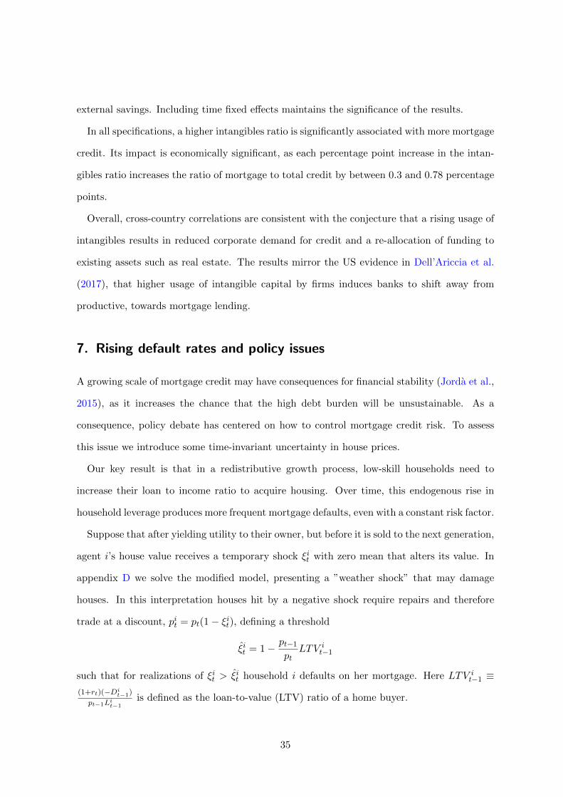
in line with our results. Finally, section 7 introduces mortgage default risk and studies policy

responses, and section 8 concludes.

2. Related literature

The paper describes how changes in factor productivity affect the allocation of income within

both the labor and capital income share, offering a neoclassical benchmark for rising inequality

3The Economist magazine (2015) stressed how technological progress favored urban locations, where real

estate prices climb under strict zoning rules.

7

(though it is not set up to describe changes in wealth distribution (Piketty, 2014)). It suggests

a key role of a rising income share of innovators (Smith et al., 2017; Koh et al., 2016), is

consistent with a rising profit share (Barkai, 2016) and an increasing wealth share for real

estate (Rognlie, 2015). The model suggests the growing productivity of intangible capital is

also a key driver for a rising savings surplus. The creation of intangible capital is largely driven

by human capital investment. Unlike physical capital, human capital cannot be purchased

(Hart and Moore, 1994). As it needs to be rewarded over time, firms can delay and thus

self finance its compensation. Research on employee compensation recognizes that short term

contracts cannot reward complex tasks. A leading survey states ”..the most common means

of rewarding white-collar workers for effort is by promotion” (Pendergast, 1999). Skilled

human capital receives direct and indirect claims on future profits via career advancement,

share and option grants. While in reality firms partially co-invest in intangible assets, a close

examination reveals that most R&D and organizational capital expenditures reflect skilled

labor compensation (Corrado and Hulten, 2010a). Even corporate brand equity may be quite

vulnerable to the departure of key employees (Rajan and Zingales, 2001).

The rise of intangible capital has also been related to the falling net leverage and increasing

cash hoardings (Falato et al., 2013). Empirical evidence suggests that firms with significant

intangibles maintain more internal resources to avoid becoming constrained, in the process

contributing to the savings glut (Dottling et al., 2017). Our approach adds to the tradi-

tional view that intangibles need to be internally financed because by their nature cannot be

pledged to investors, suggesting that the critical contractual issue is not verifiability allowed

by tangibility, but appropriability.

A fact consistent with a falling corporate demand for external finance is that the nonfinan-

cial corporate sector in most developed countries (with the exception fo France and Italy)

has progressively become a net lender (Gruber, 2015). This has led to concerns that new

technology may results in tighter financial constraints for firms Falato et al. (2013), Giglio

and Severo (2012) and Caggese and Perez-Orive (2017). Yet recent evidence suggests that

firms with more intangible capital do not appear ex ante constrained, as they have higher

8

free cash flow and do not pay out less to their shareholders (Dottling et al., 2017). This is

consistent with a rising human capital co-investment by skilled employees. Gutierrez and

Philippon (2016) find no support for rising financial frictions and evidence of industry effects

associated with globalization, competition and short termism. Alexander and Eberly (2016)

and Dottling et al. (2017) also find that both in the US and Europe weak investment is

associated with the growing role of intangible capital.

On aggregate, US listed firms have rising net equity ouflows, even since the crisis (Lazonick,

2015; Gruber, 2015). Thus overall the rise of intangible investment appears associated with

lower funding needs (a lower credit demand) rather than more binding financial constraints

(a tighter credit supply), a result consistent with record low borrowing rates.

A rising productivity of innovative human capital leads to an increasing income share for

innovators, either as start up entrepreneurs or top employees with significant outside options

(Oyer and Schaefer, 2005; Eisfeldt and Papanikolaou, 2014). As intangible value accrues

directly to its creators, it does not need to be funded by intermediaries or capital markets.

The net effect is a reduction in the supply of investables, and savings in excess of investment

that investors can appropriate.

Recent work shows a significant effect on asset pricing of shocks to the allocation of intangi-

ble value between firms and employees (Eisfeldt and Papanikolaou, 2013) or across investors

(Garlenau and Panageas, 2017). Eisfeldt and Papanikolaou (2013) develop the core idea that

key talent appropriates a large fraction of intangible value, and show how technological shocks

alter the outside option of key employees. Garlenau and Panageas (2017) study how disrup-

tive entry of new firms create unhedgeable investment risk, boosting demand for safe assets

and depressing interest rates, explaining a rising wealth share for innovators. Smith et al.

(2017) show how private business income accounts for most of the rise of top incomes since

2000, especially active owner-managers of mid-market firms in skill-intensive and unconcen-

trated industries. The key role of the owner-innovators is revealed by profit declines after a

premature death of the owner.

A related literature studies the effect of information technology on the relative productivity

9

of skilled labor to explain rising wage inequality since 1980 (e.g. see Katz and Murphy, 1992;

Autor et al., 1998, 2003). The increasing gap is in part due to a reduction in absolute real

wages for low educated workers in developed economies, a trend that cannot be explained

by a simple rise in the absolute productivity of intangibles and skilled human capital. The

assumption that skilled labor benefits most from new knowledge is consistent with Mankiw

et al. (1995). Acemoglu and Autor (2011) and other authors interpret it as the outcome

of automation of physical tasks. We show similarly that only strongly redistributive form

of technological progress can replicate all observed trends, in particular falling quantity of

price of corporate borrowing. Another likely cause is a spreading of technology to emerging

countries, leading to relocation of physical production.

Our model seeks to understand the impact of technological progress on both labor and

capital in general equilibrium. A general CES production function allows to compare how

different growth factors can account for the main trends, in particular the rise of excess savings

over productive investment. In his assessment of secular stagnation, Eichengreen (2015) finds

a fall in the relative price of investment goods a more explanation than a drop in investment

opportunities (see also Karabarbounis and Neiman, 2013; Sajedi and Thwaites, 2016). Our

setup can accommodate this interpretation, as redistributive progress leads to a fall in the

productivity-adjusted cost of physical equipment.4 Our empirical validation has focused on

showing how a redistributive technological shift represents the best parsimonious explanation

for the combination of observed economic trends. The model thus offers a technological

explanation for the rise in house prices, mortgage credit and default rates, reflecting falling

interest rates and household leverage as the general equilibrium effect of capital and labor

market trends.5 The rise in mortgage lending, household debt and default in the US has been

interpreted by country-specific factors, such as populist pressure (Rajan, 2010) or large capital

4This implies less demand for and a lower cost of physical equipment, so that the total productivity-adjusted

cost of each unit of capital falls.5As asset bubbles may well occur in equilibrium in an overlapping generation framework, the model is

consistent with speculative fluctuations around the trend.

10

inflows. Yet the share of mortgage to total credit has risen rapidly in all OECD countries

Jorda et al. (2016), and we show that its rise is related to the national adoption of intangible

investment. Dell’Ariccia et al. (2017) show how as firms increase intangibles, their creditor

banks shifts to more real estate funding.

3. Model Setup

This section describes the baseline model environment, solves the individual agents optimiza-

tion problems, and describes the equilibrium.

Time Overlapping generations live for two periods. Time starts at t = 0 and goes on to

infinity. There is an initial generation t = −1.

Goods There are two consumption goods, corn and land.6 There is a fixed amount of land

L, infinitely durable as it does not depreciate. We denote by pt the relative price of land in

terms of corn.

Households Each generation consists of a unit mass of households. Households have a

quasi-linear utility function U(ct+1, Lt) = ct+1 + v(Lt), where ct+1 denotes consumption of

corn and Lt are land holdings at the end of period t.7 The function v(L) with v′(L) > 0,

v′′(L) < 0 captures the utility households achieve from living in their house. A fraction φ

of households (i = h) is born with high human capital and offers h units of high-skill labor,

while the rest (i = l) provides l units of manual labor. Both types of labor endowments

are supplied inelastically. We assume that high-skill labor is relatively scarce, ensuring that

high-skill workers have a higher income than low-skill workers.

6We do not distinguish between houses and land, and will use the terms interchangeably.7This formulation of household preferences ensures that long-term interest rates are not pinned down by the

household’s discount factor (via an Euler equation), but instead by the relative supply of savings vehicles

versus household savings.

11

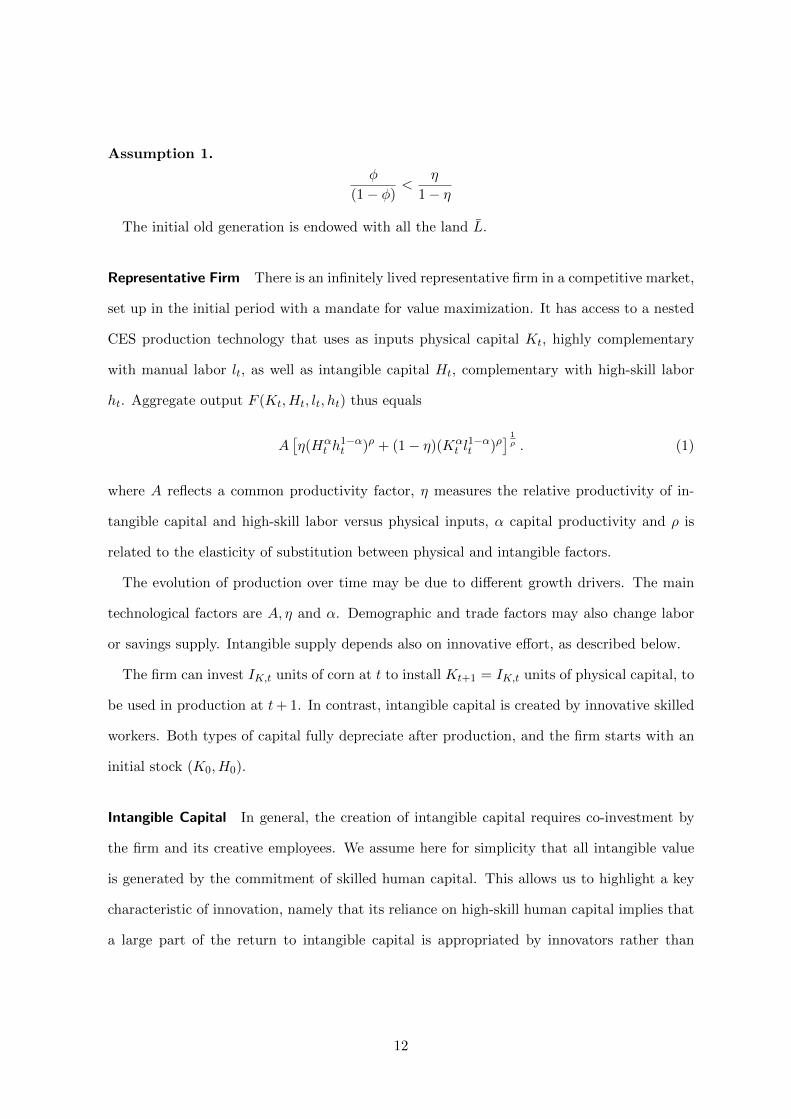
Assumption 1.

φ

(1− φ)<

η

1− η

The initial old generation is endowed with all the land L.

Representative Firm There is an infinitely lived representative firm in a competitive market,

set up in the initial period with a mandate for value maximization. It has access to a nested

CES production technology that uses as inputs physical capital Kt, highly complementary

with manual labor lt, as well as intangible capital Ht, complementary with high-skill labor

ht. Aggregate output F (Kt, Ht, lt, ht) thus equals

A[η(Hα

t h1−αt )ρ + (1− η)(Kα

t l1−αt )ρ

] 1ρ . (1)

where A reflects a common productivity factor, η measures the relative productivity of in-

tangible capital and high-skill labor versus physical inputs, α capital productivity and ρ is

related to the elasticity of substitution between physical and intangible factors.

The evolution of production over time may be due to different growth drivers. The main

technological factors are A, η and α. Demographic and trade factors may also change labor

or savings supply. Intangible supply depends also on innovative effort, as described below.

The firm can invest IK,t units of corn at t to install Kt+1 = IK,t units of physical capital, to

be used in production at t+ 1. In contrast, intangible capital is created by innovative skilled

workers. Both types of capital fully depreciate after production, and the firm starts with an

initial stock (K0, H0).

Intangible Capital In general, the creation of intangible capital requires co-investment by

the firm and its creative employees. We assume here for simplicity that all intangible value

is generated by the commitment of skilled human capital. This allows us to highlight a key

characteristic of innovation, namely that its reliance on high-skill human capital implies that

a large part of the return to intangible capital is appropriated by innovators rather than

12

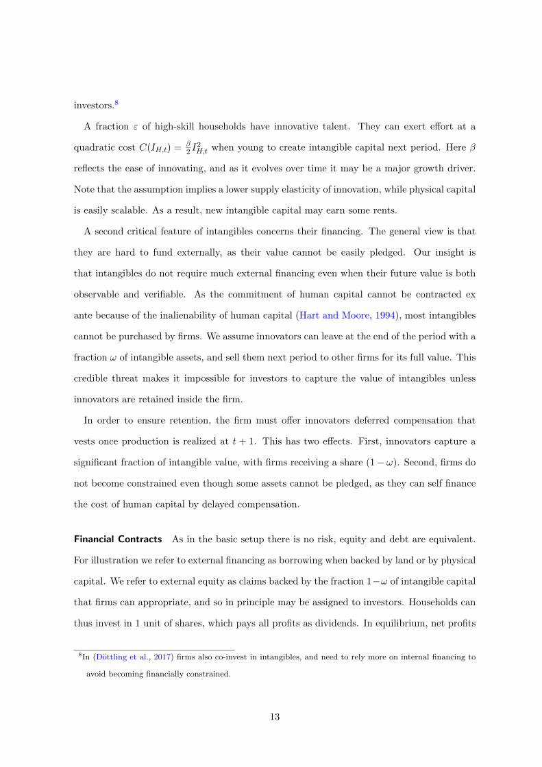
investors.8

A fraction ε of high-skill households have innovative talent. They can exert effort at a

quadratic cost C(IH,t) = β2 I

2H,t when young to create intangible capital next period. Here β

reflects the ease of innovating, and as it evolves over time it may be a major growth driver.

Note that the assumption implies a lower supply elasticity of innovation, while physical capital

is easily scalable. As a result, new intangible capital may earn some rents.

A second critical feature of intangibles concerns their financing. The general view is that

they are hard to fund externally, as their value cannot be easily pledged. Our insight is

that intangibles do not require much external financing even when their future value is both

observable and verifiable. As the commitment of human capital cannot be contracted ex

ante because of the inalienability of human capital (Hart and Moore, 1994), most intangibles

cannot be purchased by firms. We assume innovators can leave at the end of the period with a

fraction ω of intangible assets, and sell them next period to other firms for its full value. This

credible threat makes it impossible for investors to capture the value of intangibles unless

innovators are retained inside the firm.

In order to ensure retention, the firm must offer innovators deferred compensation that

vests once production is realized at t + 1. This has two effects. First, innovators capture a

significant fraction of intangible value, with firms receiving a share (1− ω). Second, firms do

not become constrained even though some assets cannot be pledged, as they can self finance

the cost of human capital by delayed compensation.

Financial Contracts As in the basic setup there is no risk, equity and debt are equivalent.

For illustration we refer to external financing as borrowing when backed by land or by physical

capital. We refer to external equity as claims backed by the fraction 1−ω of intangible capital

that firms can appropriate, and so in principle may be assigned to investors. Households can

thus invest in 1 unit of shares, which pays all profits as dividends. In equilibrium, net profits

8In (Dottling et al., 2017) firms also co-invest in intangibles, and need to rely more on internal financing to

avoid becoming financially constrained.

13

equal the appropriable revenues from intangible capital creation. Our results do not depend

on this interpretation of the firm’s capital structure. While consistent with the corporate

finance literature, it is not a direct outcome of the model. It may arise endogenously in a

model with a tax advantage for debt, in which firm income from intangible capital is a poor

source of debt collateral.

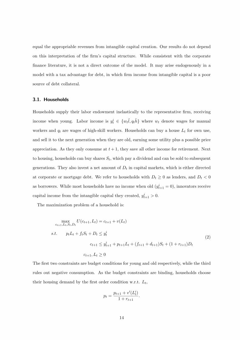
3.1. Households

Households supply their labor endowment inelastically to the representative firm, receiving

income when young. Labor income is yit ∈ {wt l, qth} where wt denote wages for manual

workers and qt are wages of high-skill workers. Households can buy a house Lt for own use,

and sell it to the next generation when they are old, earning some utility plus a possible price

appreciation. As they only consume at t+ 1, they save all other income for retirement. Next

to housing, households can buy shares St, which pay a dividend and can be sold to subsequent

generations. They also invest a net amount of Dt in capital markets, which is either directed

at corporate or mortgage debt. We refer to households with Dt ≥ 0 as lenders, and Dt < 0

as borrowers. While most households have no income when old (yit+1 = 0), innovators receive

capital income from the intangible capital they created, yit+1 > 0.

The maximization problem of a household is:

maxct+1,Lt,St,Dt

U(ct+1, Lt) = ct+1 + v(Lt)

s.t. ptLt + ftSt +Dt ≤ yit

ct+1 ≤ yit+1 + pt+1Lt + (ft+1 + dt+1)St + (1 + rt+1)Dt

ct+1, Lt ≥ 0

(2)

The first two constraints are budget conditions for young and old respectively, while the third

rules out negative consumption. As the budget constraints are binding, households choose

their housing demand by the first order condition w.r.t. Lt,

pt =pt+1 + v′(Lit)

1 + rt+1.

14

The price of housing reflects the discounted potential house price appreciation plus its

utility value. The relevant discount rate is either the mortgage interest (for a borrower) or

the opportunity cost of investing (for a lender), which in a competitive equilibrium is equal

to rt+1.

Note that housing demand is independent of income, as mortgages enable all households

to consume the same amount of housing.9 So the role of mortgage credit is to allocate land

efficiently, equalizing the marginal utility of housing across agents with heterogeneous income.

The first order condition w.r.t. St yields a pricing equation for share:

ft =ft+1 + dt1 + rt+1

. (3)

Investments in debt instruments follow as a residual Dit = yit − ftSt − ptLt. Households with

yit ≥ ptLt + ftSt have an income high enough to buy their house and invest the remainder in

shares and corporate debt. In contrast, those with yit < ptLt + ftSt need to borrow.

We focus on equilibria in which all households can afford to buy shares out of their income

and only borrow against their house, implying yit > ftSt. In this setup households with

Dit < 0 take out a mortgage loan provided by surplus households. In the absence of risk, the

intermediation process is not explicitly modelled.

3.2. Physical Capital and Labor

Firms employ labor lt and ht, and accumulate physical capital Kt, so as to maximize the

infinite stream of dividends dt:

maxKt,lt,ht

∞∑t=0

dt (4)

As investment in physical capital is financed by debt, credit demand is always equal to Kt.

Firm equity will also have positive value, since dividends can be written as

dt = F (Kt, Ht, lt, ht)− wtlt − qtht − (1 + rt)Kt − ωRtHt.

Here ωRtHt denotes the return to intangible capital appropriated by innovators, where Rt

is determined below. Under perfect competition, workers and suppliers of funding for physical

9We consider borrowing constraints in the extension on mortgage default.

15

capital are compensated according to their marginal productivity, wt = Fl,t and qt = Fh,t.

Since physical capital is fully eligible as collateral, firms are financially unconstrained and can

always scale up tangible investment until:

1 + rt = FK,t. (5)

3.3. Creation of Intangibles

A fraction of high-skill employees can exert effort to produce intangible capital for the next

period. Competitive firms are willing to pay Rt = FH,t per unit of intangible capital, reflecting

its productive value. Since the productive use of intangible capital requires the commitment of

creative human capital, innovators have a credible threat that enables them to capture some

value created.10 Firms need to match this outside option by adequate deferred compensation

equal to ωRtHt. That is, innovators capture a fraction ω of the return to the intangibles they

created.

Exerting effort innovators incur the cost C(IH,t) = β2 IH,t. They will scale up investment in

intangibles until

ωRt = βIH,t−1. (6)

As a result of a sharply increasing cost of innovation, new intangible capital earns positive

rents, unlike physical capital. Firms appropriate a fraction 1 − ω of intangible value, which

(conditional on successful retention) are verifiable and can be promised to investors. Since

production function has constant returns to scale, dividends are given by

dt = (1− ω)RtHt.

Note that the firm is never financially constrained over intangible investment, since it can

self-finance its formation by deferred equity to innovators that vest once intangible capital

produce output.

10In an alternative formulation, innovators create start up firms and sell intangible capital to other firms.

16

3.4. Equilibrium

Market clearing in the land market requires that∫ 1

0 Litdi = L. Since mortgages allow for an

efficient allocation of land, this implies Lit = L for both high-skill and manual workers.

Total net savings by households equal labor income earned by the young generation minus

their house purchases wt l+ qth− ptL. Net savings are invested in corporate debt Dt = Kt+1

and equities ft. Using that wt l+qth = (1−α)Yt, financial market clearing can thus be written

as

(1− α)Yt = ptL+ ft +Dt, (7)

where the LHS is the savings supply (labor income saved for retirement) while the RHS are

all assets that can carry savings over time, namely housing, corporate debt backed by physical

capital investment, and equity backed by the return on intangibles captured by firms.

3.5. Steady State

Our goal is to study the long-term impact of different drivers behind the growth process in our

model. To that end, it is useful to briefly consider how the relative importance of intangible

capital affects the steady state allocation in our model.

From financial market clearing (7) it is clear that households save a constant fraction (1−α)

of income. Our main focus is how these savings are allocated to the three savings vehicles in

our model. In steady state, share prices and house prices can be written as

f =(1− ω)RH

r, (8)

p =v′(L)

r. (9)

Both these long-term assets increase in value as interest rates fall. The value of intangibles

is another determinant of share prices.

As the relative role of intangible capital in the economy grows, firms demand relatively less

external finance in the form of corporate debt, which is backed by physical capital. Some of

the excess savings are absorbed by share prices, which rise in value as the return on intangibles

17

increases. However, as investors only appropriate a fraction (1−ω) of the return to intangibles,

innovators receive a rising share of total income. As an increasing share of the capital stock

is not investable, excess savings push down interest rates and boost land prices.

4. Secular trends

We now analyze alternative formulations of the growth process to assess what factors can

best explain the evolution of economic trends since the 1980s. After identifying the main

trends, we analyze analytically and quantitatively individual growth factors. Our main focus

is on technological progress, but we also consider globalization and social trends such as

demographics and rising education levels.

While some factors can account for some subset of trends, we find that only a strongly

redistributive form of technological progress can drive the combination of overall growth,

falling investment and interest rates. This set of core results in turn can produce all other

trends. After showing this result analytically, we evaluate empirically this interpretation by

a quantification exercise.

4.1. Major secular trends

This section lists major economic trends over the past 35 years, that a broadly specified

growth model should be able to explain.

Falling real interest rates Real rates have gradually fallen across advanced economies since

the early 1980s (King and Low, 2014). For the U.S. we compute the real interest rate as the

10 year treasury yield minus inflation.11 From a peak above 8% in the early 1980s, US real

rates have steadily been declining, to a level around 0% in recent years.

11Both series are downloaded from FRED.

18

Rising intangible relative to tangible investment Corporate investment in intangible assets

has risen while physical investment has declined (Corrado and Hulten, 2010b).12

We compute the ratio of intangible to total capital for the US economy aggregating firm-

level data from Compustat, combined with the measure of intangible capital of Peters and

Taylor (2017).13 We also compute the intangibles ratio from national accounts using data

from the BEA’s NIPA tables.

Figure 1 in the introduction plots the estimated intangible ratio from these two sources.

The Compustat intangibles ratio is on a higher level, since the approach by Peters and Taylor

(2017) capitalizes more spending flows than the BEA. For example, the BEA measure does

not capitalize any SG&A spending that contributes to a firm’s organizational structure. Im-

portantly for us, there is a clear upward trend in both series, highlighting the growing role of

intangible capital across data sources. In our model, this trend is represented by a growing

value of H relative to K.

Decreasing corporate net borrowing US corporations have been reducing their net bor-

rowing and repurchasing more shares than they issued. The left panel of figure 3 replicates

the drop in corporate net leverage of Compustat firms in Bates et al. (2009), next to own

calculations showing how the decrease is concentrated among firms with the most intangi-

ble assets.14 Among others, Lazonick (2015) shows how U.S. firms experienced net equity

12Intangible capital is here defined as the capitalization of expert human capital invested in corporate knowl-

edge, organizational capability, computerized information and internal software.13This approach capitalizes R&D and some SG&A expenses, as they represent investments in knowledge

capital, organizational structure, and brand equity. We then define the aggregate intangible ratio as the

ratio of aggregate intangible capital relative to aggregate total (physical plus intangible) capital. Physical

capital is defined as property plant and equipment (PPENT). Computing this metric, we restrict the sample

to firms with non-missing and at least $1m in total assets. We also exclude financial firms (SIC codes 6000

- 6999) and utilities (SIC codes 4900 - 4999).14The figure plots average total debt (DLTT + DLC) net of cash holdings (CHE) scaled by assets (AT) for

Compustat firms. HINT firms are in the highest tercile of the intangibles ratio distribution in a given year,

while LINT are in the lowest tercile.

19

Figure 3: Net leverage and borrowing by non-financial corporations

outflows since 1980, even after the recent crisis.

This overall decrease in external financing by corporations is further confirmed by data

on net borrowing of US non-financial businesses from the Flow of Funds, scaled by nominal

GDP.15 This series is plotted in the right panel of figure 3, and displays an even sharper

downward trend. This is puzzling as a fall in real rates reduces the marginal cost of tangible

investment and borrowing.

Note that consistently with the corporate finance literature, we interpret external financing

for tangible investment K as debt. For comparison, the right panel of figure 3 also plots

BEA data on non-residential, non-IPP investment relative to GDP, which can also represent

K/Y in our model. Both series exhibit an overall downward trend. Therefore, technological

progress should be able to account for a falling KY in our model.

Mortgage credit growth In contrast to falling corporate credit, mortgage credit has shown

a steady rise relative to GDP, as figure 4 shows using data from the Flow of Funds.16 While

15This series is defined as total liabilities minus total financial assets.16The left panel plots aggregate home mortgage credit by households. This series is derived from the Flow of

Funds and defined as the total amount of home mortgage debt outstanding by households and nonprofit

organizations, divided by nominal GDP. The right panel plots land values computed by (Davis and Heath-

cote, 2007), divided by nominal GDP. The red dashed line plots the trend components with an HP filter

with smoothing parameter 1600.

20

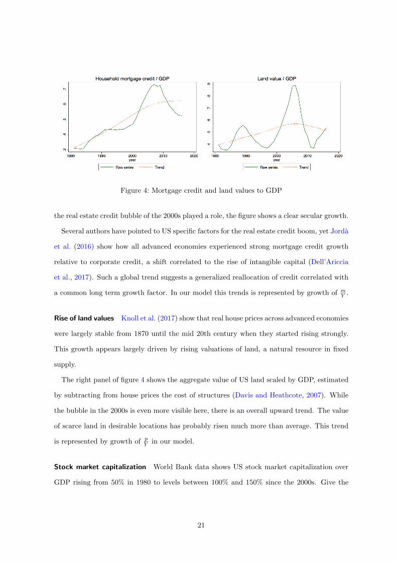
Figure 4: Mortgage credit and land values to GDP

the real estate credit bubble of the 2000s played a role, the figure shows a clear secular growth.

Several authors have pointed to US specific factors for the real estate credit boom, yet Jorda

et al. (2016) show how all advanced economies experienced strong mortgage credit growth

relative to corporate credit, a shift correlated to the rise of intangible capital (Dell’Ariccia

et al., 2017). Such a global trend suggests a generalized reallocation of credit correlated with

a common long term growth factor. In our model this trends is represented by growth of mY .

Rise of land values Knoll et al. (2017) show that real house prices across advanced economies

were largely stable from 1870 until the mid 20th century when they started rising strongly.

This growth appears largely driven by rising valuations of land, a natural resource in fixed

supply.

The right panel of figure 4 shows the aggregate value of US land scaled by GDP, estimated

by subtracting from house prices the cost of structures (Davis and Heathcote, 2007). While

the bubble in the 2000s is even more visible here, there is an overall upward trend. The value

of scarce land in desirable locations has probably risen much more than average. This trend

is represented by growth of pY in our model.

Stock market capitalization World Bank data shows US stock market capitalization over

GDP rising from 50% in 1980 to levels between 100% and 150% since the 2000s. Give the

21

evidence on large net equity outflows, this suggests a significant revaluation effect driven

by lower rates and rising profits. In the model this value is measured by fY , the value of

outstanding shares relative to income.

Rising wage inequality Survey data from the US Bureau of Labor Statistics show a sharp

increase in relative earnings of workers with at least a Bachelor degree since 1980. This skill

premium trend has been interpreted as the result of skill-biased technological change com-

plementary with high cognitive skills that replaces low skill functions (Acemoglu and Autor,

2011). It is represented by an increase in qw in the context of our model.

This list defines a set of trends that we seek to explain in the context of our model,

T ={r ↓, H

H+K ↑,KY ↓,

mY ↑,

pY ↑,

fY ↑,

qw ↓}

.

4.2. Key growth drivers

What parsimonious description of the growth progress can at best reproduce these secular

trends? Our general production function suggests some technological explanations. A uniform

growth effect driven by a rising common productivity factor A as in the classic Solow model

benefits all factors of production indiscriminatingly, and is inconsistent with the growing role

of intangible capital and high-skill workers.

Accordingly, we focus on intangible-biased growth drivers, and only adjust the common

technological progress component A in our quantitative exercise to match the overall level of

growth.

• An IT-induced reduction in the cost of producing intangible capital (a fall in β) is a

natural growth driver. It boosts the supply of intangible capital relative to physical

investment, and leads to higher rewards for complementary factors such as skilled la-

bor. A higher intangible capital creation also implies more total income accruing to

innovators. This form of progress is weakly redistributive, as it benefits indirectly also

physical factors through their complementarity.

22

• A more redistributive shift would interpret technological progress as a strong rise in

the productivity of intangible capital and skilled labor relative to physical capital and

labor at the technological frontier. Such a rise in η leads to aggregate income growth

provided there is sufficient skilled labor supply. In this formulation, the absolute pro-

ductivity of some factors in the optimal productive combination (1) may actually fall

over time, consistent with the notion that new technologies replace physical labor at

the technological frontier (Acemoglu and Autor, 2011).17

Given the evidence on a growing role of intangible capital, our focus is on technological

growth drivers. However, economic trends certainly reflect multiple causes, and we also

consider other relevant factors. We list here the drivers that we can directly study in our

model:

• The share of university educated workers has risen steadily in recent decades. More

skilled labor may explain a growing supply of intangible capital. This process is de-

scribed by an exogenous increase of φ, the fraction of skilled labor.

• Piketty (2014) highlights a historical fall in the labor share since the 1970s. This is a

redistributive factor that may explain some observed changes in the income distribution.

In our model it can be the results of a rising technological importance of capital α in

our model.

• A rising ω would reflect an increased bargaining power for innovators over corporations.

This factor may boost intangible capital and reduce the investment opportunities avail-

able to the public.

• A savings glut with significant capital inflows from abroad may have contributed to the

rise of housing prices and mortgage credit in the US. To study capital inflows in our

model, suppose foreigners invest a fraction xt of GDP in domestic financial claims. As

they live abroad, foreigners do not gain utility from housing, so holding land directly

17As we discuss later, this effect is reinforced by globalization of production as the result of knowledge spillovers.

23

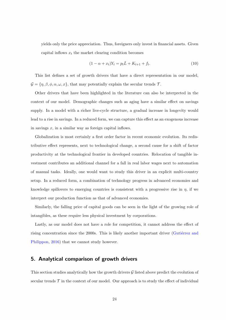
yields only the price appreciation. Thus, foreigners only invest in financial assets. Given

capital inflows xt the market clearing condition becomes

(1− α+ xt)Yt = ptL+Kt+1 + ft. (10)

This list defines a set of growth drivers that have a direct representation in our model,

G = {η, β, φ, α, ω, x}, that may potentially explain the secular trends T .

Other drivers that have been highlighted in the literature can also be interpreted in the

context of our model. Demographic changes such as aging have a similar effect on savings

supply. In a model with a richer live-cycle structure, a gradual increase in longevity would

lead to a rise in savings. In a reduced form, we can capture this effect as an exogenous increase

in savings x, in a similar way as foreign capital inflows.

Globalization is most certainly a first order factor in recent economic evolution. Its redis-

tributive effect represents, next to technological change, a second cause for a shift of factor

productivity at the technological frontier in developed countries. Relocation of tangible in-

vestment contributes an additional channel for a fall in real labor wages next to automation

of manual tasks. Ideally, one would want to study this driver in an explicit multi-country

setup. In a reduced form, a combination of technology progress in advanced economies and

knowledge spillovers to emerging countries is consistent with a progressive rise in η, if we

interpret our production function as that of advanced economies.

Similarly, the falling price of capital goods can be seen in the light of the growing role of

intangibles, as these require less physical investment by corporations.

Lastly, as our model does not have a role for competition, it cannot address the effect of

rising concentration since the 2000s. This is likely another important driver (Gutierrez and

Philippon, 2016) that we cannot study however.

5. Analytical comparison of growth drivers

This section studies analytically how the growth drivers G listed above predict the evolution of

secular trends T in the context of our model. Our approach is to study the effect of individual

24

drivers on the economy’s long-run allocation. This comparative static exercise assumes an

initial steady state around 1980, and a final steady state around 2015. Section 6 complements

this approach by calibrating the model and calculating the combined effect of different factors

across steady states. At this point we also simulate the perfect-foresight path between the

two long-run allocations.

5.1. Analytical results

For our analytical results we restrict attention to the Cobb-Douglas case (the limiting case

once ρ→ 0, see appendix A for the general CES case). We start with a simple observation:

Observation. To individually explain all secular trends T simultaneously, any growth driver

must be able to explain falling corporate borrowing and physical investment DY = K

Y , along

with falling interest rates r.

This observation conveys a simple intuition. Any driver behind the observed trends must

explain a simultaneous drop in the quantity and price of external finance.

Falling corporate net borrowing and interest rates are directly manifested in the data.

Moreover, in the model the financial market clearing condition (7) shows clearly that a rising

KY requires either p

Y or fY to be decreasing, directly contradicting their observed trend.

(1− α) =p

YL+

f

Y+K

Y.

This observation mirrors the insight in the labor literature that rising wage inequality

coupled with an increase in high-skill employment must be the result of growing demand for

skilled workers (e.g. Autor et al., 1998).

After this useful insight we can state our main result:

Theorem. Among all growth drivers in the set G, only a strongly redistributional form of

technological progress (defined as an increase of η) can produce simultaneously all the observed

trends T .

25

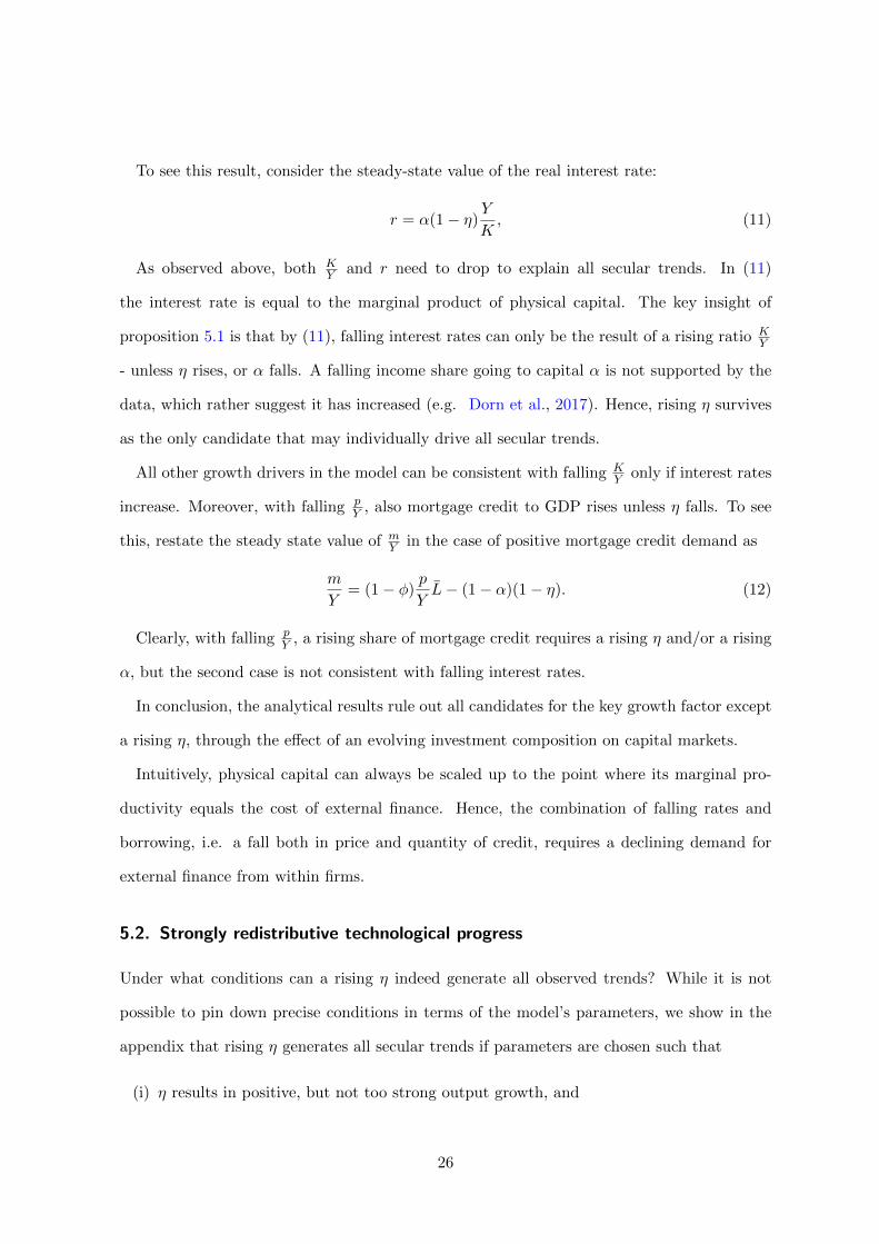
To see this result, consider the steady-state value of the real interest rate:

r = α(1− η)Y

K, (11)

As observed above, both KY and r need to drop to explain all secular trends. In (11)

the interest rate is equal to the marginal product of physical capital. The key insight of

proposition 5.1 is that by (11), falling interest rates can only be the result of a rising ratio KY

- unless η rises, or α falls. A falling income share going to capital α is not supported by the

data, which rather suggest it has increased (e.g. Dorn et al., 2017). Hence, rising η survives

as the only candidate that may individually drive all secular trends.

All other growth drivers in the model can be consistent with falling KY only if interest rates

increase. Moreover, with falling pY , also mortgage credit to GDP rises unless η falls. To see

this, restate the steady state value of mY in the case of positive mortgage credit demand as

m

Y= (1− φ)

p

YL− (1− α)(1− η). (12)

Clearly, with falling pY , a rising share of mortgage credit requires a rising η and/or a rising

α, but the second case is not consistent with falling interest rates.

In conclusion, the analytical results rule out all candidates for the key growth factor except

a rising η, through the effect of an evolving investment composition on capital markets.

Intuitively, physical capital can always be scaled up to the point where its marginal pro-

ductivity equals the cost of external finance. Hence, the combination of falling rates and

borrowing, i.e. a fall both in price and quantity of credit, requires a declining demand for

external finance from within firms.

5.2. Strongly redistributive technological progress

Under what conditions can a rising η indeed generate all observed trends? While it is not

possible to pin down precise conditions in terms of the model’s parameters, we show in the

appendix that rising η generates all secular trends if parameters are chosen such that

(i) η results in positive, but not too strong output growth, and

26

(ii) ω is sufficiently large.

While a rising η implies directly a decreasing relative productivity of K, by general comple-

mentarity all factors benefit from overall output growth. Provided the effect of η on growth

is not too strong the direct effect dominates, resulting in a falling equilibrium ratio of KY .

When rising η results in falling KY , firms demand less external financing, and excess savings

are absorbed by land and share prices. As long as ω is not too large, most of the returns to

innovation are captured by human capital, and hence do not constitute a savings vehicle for

the general public. As a result, the growth in stock prices is limited and land values rise to

absorb some of the slack savings.18

To summarize, strongly redistributive technological progress shifts firm investment to in-

tangible capital, inducing a fall in their external financing needs. As long as overall growth

is not too strong, firms decrease their leverage despite falling interest rates. It also results in

increasing house and share prices, a rising ratio of mortgage to productive credit and more

wage inequality.

6. Calibration and Empirical Validation

We now run a quantitative exercise on our model to see how well different drivers can explain

the observed trends in U.S. data. To that end, we calibrate our economy to 1980 and change

individual drivers to match the evolution of the intangible-tangible ratio over time. We

then compare the evolution of unmatched endogenous variables to the data, to see how well

individual drivers explain those trends.

While our model is not suited for a full-blown quantitative assessment of different drivers,

this exercise still allows us to get a sense of the magnitude of the effects. It also allows us to

elaborate in more detail why drivers other than η fail.

While a redistributive technological shift η emerges as the best growth driver able to explain

individually the evolution of investment, economic trends certainly reflect multiple causes.

18If ω were small most intangible value is reflected in shares, absorbing savings.

27

Accordingly, we also use our calibration to assess the joint effect of multiple drivers. While

capital inflows and rising education levels can help explain the magnitude of trends, a shift

towards intangibles still emerges as a necessary driver to explain why corporations borrow

less in the light of low interest rates.

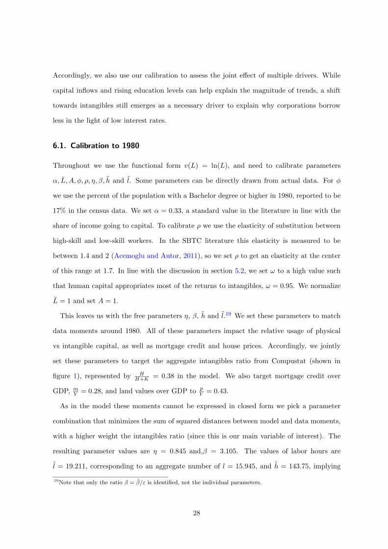
6.1. Calibration to 1980

Throughout we use the functional form v(L) = ln(L), and need to calibrate parameters

α, L, A, φ, ρ, η, β, h and l. Some parameters can be directly drawn from actual data. For φ

we use the percent of the population with a Bachelor degree or higher in 1980, reported to be

17% in the census data. We set α = 0.33, a standard value in the literature in line with the

share of income going to capital. To calibrate ρ we use the elasticity of substitution between

high-skill and low-skill workers. In the SBTC literature this elasticity is measured to be

between 1.4 and 2 (Acemoglu and Autor, 2011), so we set ρ to get an elasticity at the center

of this range at 1.7. In line with the discussion in section 5.2, we set ω to a high value such

that human capital appropriates most of the returns to intangibles, ω = 0.95. We normalize

L = 1 and set A = 1.

This leaves us with the free parameters η, β, h and l.19 We set these parameters to match

data moments around 1980. All of these parameters impact the relative usage of physical

vs intangible capital, as well as mortgage credit and house prices. Accordingly, we jointly

set these parameters to target the aggregate intangibles ratio from Compustat (shown in

figure 1), represented by HH+K = 0.38 in the model. We also target mortgage credit over

GDP, mY = 0.28, and land values over GDP to p

Y = 0.43.

As in the model these moments cannot be expressed in closed form we pick a parameter

combination that minimizes the sum of squared distances between model and data moments,

with a higher weight the intangibles ratio (since this is our main variable of interest). The

resulting parameter values are η = 0.845 and,β = 3.105. The values of labor hours are

l = 19.211, corresponding to an aggregate number of l = 15.945, and h = 143.75, implying

19Note that only the ratio β = β/ε is identified, not the individual parameters.

28

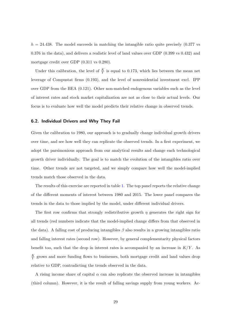
h = 24.438. The model succeeds in matching the intangible ratio quite precisely (0.377 vs

0.376 in the data), and delivers a realistic level of land values over GDP (0.399 vs 0.432) and

mortgage credit over GDP (0.311 vs 0.280).

Under this calibration, the level of KY is equal to 0.173, which lies between the mean net

leverage of Compustat firms (0.193), and the level of nonresidential investment excl. IPP

over GDP from the BEA (0.121). Other non-matched endogenous variables such as the level

of interest rates and stock market capitalization are not as close to their actual levels. Our

focus is to evaluate how well the model predicts their relative change in observed trends.

6.2. Individual Drivers and Why They Fail

Given the calibration to 1980, our approach is to gradually change individual growth drivers

over time, and see how well they can replicate the observed trends. In a first experiment, we

adopt the parsimonious approach from our analytical results and change each technological

growth driver individually. The goal is to match the evolution of the intangibles ratio over

time. Other trends are not targeted, and we simply compare how well the model-implied

trends match those observed in the data.

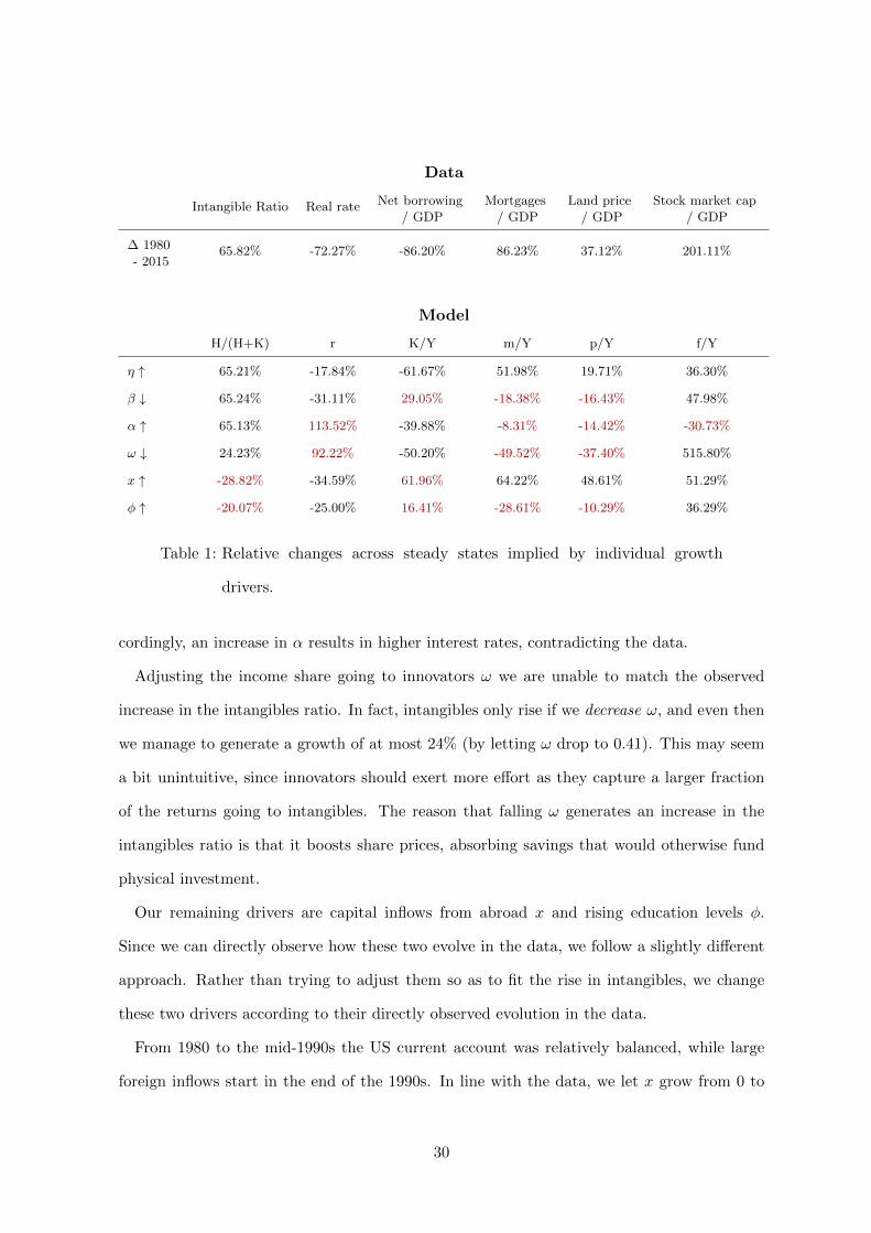
The results of this exercise are reported in table 1. The top panel reports the relative change

of the different moments of interest between 1980 and 2015. The lower panel compares the

trends in the data to those implied by the model, under different individual drivers.

The first row confirms that strongly redistributive growth η generates the right sign for

all trends (red numbers indicate that the model-implied change differs from that observed in

the data). A falling cost of producing intangibles β also results in a growing intangibles ratio

and falling interest rates (second row). However, by general complementarity physical factors

benefit too, such that the drop in interest rates is accompanied by an increase in K/Y . As

KY grows and more funding flows to businesses, both mortgage credit and land values drop

relative to GDP, contradicting the trends observed in the data.

A rising income share of capital α can also replicate the observed increase in intangibles

(third column). However, it is the result of falling savings supply from young workers. Ac-

29

Data

Intangible Ratio Real rate Net borrowing

/ GDP

Mortgages

/ GDP

Land price

/ GDP

Stock market cap

/ GDP

∆ 1980

- 201565.82% -72.27% -86.20% 86.23% 37.12% 201.11%

Model

H/(H+K) r K/Y m/Y p/Y f/Y

η ↑ 65.21% -17.84% -61.67% 51.98% 19.71% 36.30%

β ↓ 65.24% -31.11% 29.05% -18.38% -16.43% 47.98%

α ↑ 65.13% 113.52% -39.88% -8.31% -14.42% -30.73%

ω ↓ 24.23% 92.22% -50.20% -49.52% -37.40% 515.80%

x ↑ -28.82% -34.59% 61.96% 64.22% 48.61% 51.29%

φ ↑ -20.07% -25.00% 16.41% -28.61% -10.29% 36.29%

Table 1: Relative changes across steady states implied by individual growth

drivers.

cordingly, an increase in α results in higher interest rates, contradicting the data.

Adjusting the income share going to innovators ω we are unable to match the observed

increase in the intangibles ratio. In fact, intangibles only rise if we decrease ω, and even then

we manage to generate a growth of at most 24% (by letting ω drop to 0.41). This may seem

a bit unintuitive, since innovators should exert more effort as they capture a larger fraction

of the returns going to intangibles. The reason that falling ω generates an increase in the

intangibles ratio is that it boosts share prices, absorbing savings that would otherwise fund

physical investment.

Our remaining drivers are capital inflows from abroad x and rising education levels φ.

Since we can directly observe how these two evolve in the data, we follow a slightly different

approach. Rather than trying to adjust them so as to fit the rise in intangibles, we change

these two drivers according to their directly observed evolution in the data.

From 1980 to the mid-1990s the US current account was relatively balanced, while large

foreign inflows start in the end of the 1990s. In line with the data, we let x grow from 0 to

30

Data

Intangible

RatioReal GDP Real rate Net borrowing

/ GDP

Mortgages

/ GDP

Land price

/ GDP

Market cap

/ GDP

∆ 1980

- 201565.82% 140.82% -72.27% -86.20% 86.23% 37.12% 201.11%

Model

H/(H+K) Y r K/Y m/Y p/Y f/Y

η +A, φ, x 64.98% 140.78% -75.04% -74.52% 89.38% 66.42% 366.30%

β +A, φ, x 65.14% 140.88% -64.14% 107.33% 6.17% 15.78% 47.98%

α+A, φ, x 63.61% -48.84% 31.28% -14.55% 49.48% 48.90% 14.82%

ω +A, φ, x 51.90% -40.12% 43.81% -46.99% 5.87% 16.12% 727.73%

Table 2: Relative changes across steady states implied by combination of growth

drivers.

0.35 in the final steady state. While a savings glut pushes down interest rates, by itself it

cannot explain why foreign funding did not flow to corporations to fund physical investment.

Finally, we adjust the fraction of high-skill households from φ = 0.17 in 1980, to φ = 0.3 in

2015, in line with the evolution of the fraction of the U.S. population with a Bachelor degree

or higher. Higher incomes increase the savings supply, which pushes down interest rates but

also flows to firms and investment in physical capital.

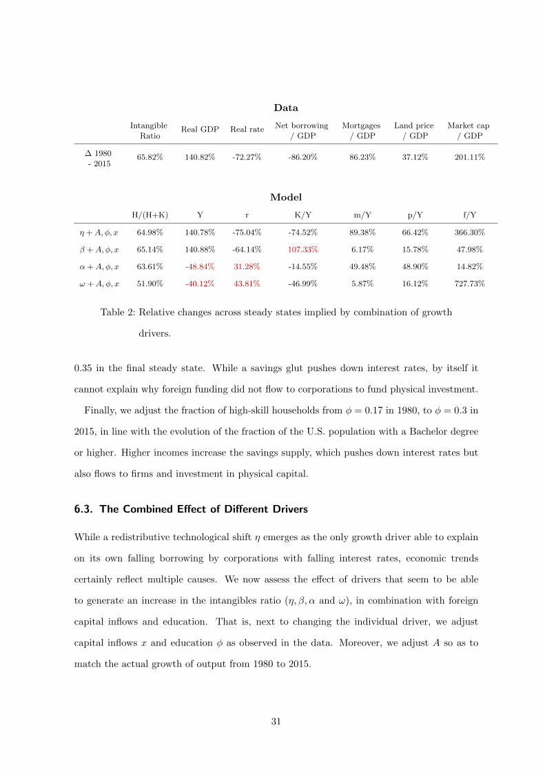
6.3. The Combined Effect of Different Drivers

While a redistributive technological shift η emerges as the only growth driver able to explain

on its own falling borrowing by corporations with falling interest rates, economic trends

certainly reflect multiple causes. We now assess the effect of drivers that seem to be able

to generate an increase in the intangibles ratio (η, β, α and ω), in combination with foreign

capital inflows and education. That is, next to changing the individual driver, we adjust

capital inflows x and education φ as observed in the data. Moreover, we adjust A so as to

match the actual growth of output from 1980 to 2015.

31

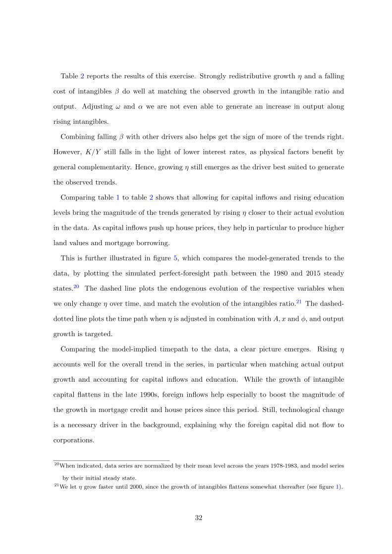
Table 2 reports the results of this exercise. Strongly redistributive growth η and a falling

cost of intangibles β do well at matching the observed growth in the intangible ratio and

output. Adjusting ω and α we are not even able to generate an increase in output along

rising intangibles.

Combining falling β with other drivers also helps get the sign of more of the trends right.

However, K/Y still falls in the light of lower interest rates, as physical factors benefit by

general complementarity. Hence, growing η still emerges as the driver best suited to generate

the observed trends.

Comparing table 1 to table 2 shows that allowing for capital inflows and rising education

levels bring the magnitude of the trends generated by rising η closer to their actual evolution

in the data. As capital inflows push up house prices, they help in particular to produce higher

land values and mortgage borrowing.

This is further illustrated in figure 5, which compares the model-generated trends to the

data, by plotting the simulated perfect-foresight path between the 1980 and 2015 steady

states.20 The dashed line plots the endogenous evolution of the respective variables when

we only change η over time, and match the evolution of the intangibles ratio.21 The dashed-

dotted line plots the time path when η is adjusted in combination with A, x and φ, and output

growth is targeted.

Comparing the model-implied timepath to the data, a clear picture emerges. Rising η

accounts well for the overall trend in the series, in particular when matching actual output

growth and accounting for capital inflows and education. While the growth of intangible

capital flattens in the late 1990s, foreign inflows help especially to boost the magnitude of

the growth in mortgage credit and house prices since this period. Still, technological change

is a necessary driver in the background, explaining why the foreign capital did not flow to

corporations.

20When indicated, data series are normalized by their mean level across the years 1978-1983, and model series

by their initial steady state.21We let η grow faster until 2000, since the growth of intangibles flattens somewhat thereafter (see figure 1).

32

Figure 5: Simulated perfect-foresight time path compared to actual series.

Actual series are naturally more volatile since our long term approach cannot match os-

cillations around trends. This is particularly visible in the land price and mortgage credit

series during the real estate bubble in the 2000s. Overall, given our simple model and given

that we do not match any trends other than the intangibles ratio and output growth, the

model-generated series are relatively close to the underlying trend in the data.

6.4. Cross-country evidence

According to the model, excess savings driven by intangible use by firms boost mortgage credit

over GDP. We further examine this empirical relationship in a panel of OECD countries,

seeking to explain the share of mortgage credit to total credit calculated by Jorda et al.

(2016).

33

Table 3: Cross country evidence on mortgage credit and intangible investment

Mortgage Ratio is the ratio of mortgage to total credit. Intangibles Ratio is the ratio of intan-

gibles to total assets. Reported t-statistics based on errors clustered at the firm level. ***, **,

* indicate significance at 1%, 5%, and 10% level. All independent variables are lagged one year.

(1) (2) (3) (4)

Mortgage Ratio Mortgage Ratio Mortgage Ratio Mortgage Ratio

Intangibles Ratio (INTAN-Invest) 0.777∗∗∗ 0.706∗∗∗

(5.00) (4.05)

Intangibles Ratio (Compustat) 0.299∗∗∗ 0.432∗∗∗

(3.29) (3.34)

Log GDP per capita 0.00360 -0.870

(0.04) (-1.70)

Current Account 0.00175 0.00928

(0.40) (1.37)

Year Fixed Effects No Yes No Yes

Observations 263 263 264 264

Adjusted R2 0.402 0.392 0.152 0.270

t statistics in parentheses

∗ p < 0.10, ∗∗ p < 0.05, ∗∗∗ p < 0.01

We use the intangible capital measures based on National Accounts, available through the

INTAN-Invest project (see Corrado et al., 2012). As an alternative measure we use Compu-

stat Global firm data, estimating intangibles by capitalizing R&D and SG&A expenditures

as in Dottling et al. (2017) and Peters and Taylor (2016).22

Table 3 presents the results of fixed effect and pooled OLS regressions using the two intan-

gible ratio measures, GDP per capita as a general control and capital inflows to include net

22For details see Dottling et al. (2017). Compustat Global data coverage is from 1989 to 2015, the INTAN-

Invest series from 1995 to 2010. These measures are strongly correlated, with an average of 0.82.

34

external savings. Including time fixed effects maintains the significance of the results.

In all specifications, a higher intangibles ratio is significantly associated with more mortgage

credit. Its impact is economically significant, as each percentage point increase in the intan-

gibles ratio increases the ratio of mortgage to total credit by between 0.3 and 0.78 percentage

points.

Overall, cross-country correlations are consistent with the conjecture that a rising usage of

intangibles results in reduced corporate demand for credit and a re-allocation of funding to

existing assets such as real estate. The results mirror the US evidence in Dell’Ariccia et al.

(2017), that higher usage of intangible capital by firms induces banks to shift away from

productive, towards mortgage lending.

7. Rising default rates and policy issues

A growing scale of mortgage credit may have consequences for financial stability (Jorda et al.,

2015), as it increases the chance that the high debt burden will be unsustainable. As a

consequence, policy debate has centered on how to control mortgage credit risk. To assess

this issue we introduce some time-invariant uncertainty in house prices.

Our key result is that in a redistributive growth process, low-skill households need to

increase their loan to income ratio to acquire housing. Over time, this endogenous rise in

household leverage produces more frequent mortgage defaults, even with a constant risk factor.

Suppose that after yielding utility to their owner, but before it is sold to the next generation,

agent i’s house value receives a temporary shock ξit with zero mean that alters its value. In

appendix D we solve the modified model, presenting a ”weather shock” that may damage

houses. In this interpretation houses hit by a negative shock require repairs and therefore

trade at a discount, pit = pt(1− ξit), defining a threshold

ξit = 1− pt−1

ptLTV i

t−1

such that for realizations of ξit > ξit household i defaults on her mortgage. Here LTV it−1 ≡

(1+rt)(−Dit−1)

pt−1Lit−1is defined as the loan-to-value (LTV) ratio of a home buyer.

35

As shown in the appendix, a stationary shock leaves the equilibrium allocation unchanged.

As a result we immediately have the following corollary:

Corollary 1. Define χt ≡ 1−G(ξlt) as the aggregate default of low-skill workers. Technological

progress that results in rising mortgage credit relative to GDP also produces increasing steady-

state default among low-skill workers (dχdη ≥ 0)

As technological progress increases income inequality and house prices, low-skill workers

end up with higher LTV-ratios, lowering the threshold ξl. Thus even for a given distribution

of shocks, default occurs more frequently.

While rising mortgage default rates were a main cause for the 2008 financial crisis, in our

current formulation any default is just an ex-post transfer with no aggregate welfare loss.

As lenders are compensated by a higher interest rate, there is no inefficiency that needs to

be addressed by a Pareto-improving policy intervention, since the economy is dynamically

efficient. If however mortgage defaults caused a financial externality, e.g. through fire sales

(Lorenzoni, 2008) or aggregate demand externalities (Korinek and Simsek, 2016), stronger

policy intervention over time may be warranted, for example through tightening loan-to-value

ratios.

Such a policy has interesting side effects for the long run allocation in our model. Restrain-

ing the borrowing of young home buyers restricts their ability to bid up the price of land,

reducing house prices while pushing interest rates even lower. As the released savings are

redirected towards physical investment, in general equilibrium both output and wages grow

via the indirect subsidy to production. The trade off is that the old generation suffers a capi-

tal loss, and the stock of housing is allocated less efficiently. Interestingly, the policy benefits

most those for whom the borrowing constraint becomes binding. Young low-skill workers gain

through smaller transfers to older generations and a higher capital stock - a consequence of

lower equilibrium land prices.23

This result mirrors Deaton and Laroque (2001), who show that introducing land in a base-

23We derive these results formally and they are available upon request.

36

line OLG growth model eliminates the ”Golden Rule” steady state that maximizes long-run

consumption. As land absorbs savings, there is generally an under-accumulation of produc-

tive capital. Our model highlights that this effect may be stronger in a knowledge economy

where capital is becoming more intangible-intensive over time.

8. Conclusion

This paper offers a neoclassical growth model where technological change can account for the

growing excess of savings over productive investment sometimes dubbed as ”secular stagna-

tion”.

While skill-biased technological progress is known to explain the evolution of relative wages,

our framework extends it to derive concomitant trends in credit allocation and asset prices. A

boost to the productivity of intangible investment increases the value captured by innovators

who invest their own human capital, resulting in a fall in corporate demand for finance. The

savings glut progressively lowers interest rates, leading to repricing of long term assets such

as houses and shares.

The model can endogenize popular explanations for a persistent period of low investment,

such as a drop in investment opportunities and a fall in the relative price of investment

goods. As Cochrane (1994) highlights, evolution in corporate investment may reflect other

economic forces besides technological improvements. The model is able to incorporate also

nontechnological factors, such as the effect of globalization on labor supply and the relocation

of production. The savings surplus is certainly affected by savings supply shocks driven by

demographic changes and capital outflows from emerging markets, although such nontech-

nological factors cannot explain all economic trends (Eichengreen, 2015). In particular, the

contemporaneous drop in interest rates and tangible investment requires a drop in credit

demand rather than a boost to credit supply.

Our redistributive growth model is aimed specifically at explaining the evidence on de-

veloped countries rather than describing a global production function. Thus the evolution

37

of relative factor productivity is reinforced by globalization, where advanced economies spe-

cialize in high intangible industries while some physical production is relocated to emerging

markets. This shift in comparative advantage may reflect a gradual knowledge spillover that

induces developed economies to specialize in innovative products to maintain growth. The

process has redistributive effects on physical and skilled labor as well as on the allocation of

intangible capital return between innovators and investors.

Critically, excess savings arise because savers cannot co-invest in the private development

of intangible capital (Hart and Moore, 1994). Innovative entrepreneurs are nowadays largely

self financed, as they need only modest upfront investment and can fund skilled human capital

investment via deferred compensation and equity grants. Anecdotal evidence suggests that

a large fraction of value created by innovative firms accrues to founders and employees, and

these firms maintain a steady share dilution rate via equity grants to employees. The fall in

investable and falling rates induces a shift to other long term investment such as housing.

Rognlie (2015) confirms that surging house prices account for a rising fraction of the capital

share of aggregate income.

In conclusion, our framing enables to assess what form of technological progress can best

account for major secular trends. While in the classic Solow growth model (Solow, 1956)

progress boosts equally all factors’ productivity, IT has clearly favored some factors. Our

evidence suggests that the trends cannot be explained simply by a rise in the productivity

of intangibles. Only a highly redistributive reallocation of productivity can account for the

observed trends, in particular with the combination of a steady fall in physical investment,

falling interest rates and labor wages in a context of aggregate growth (Acemoglu and Autor,

2011).

Overall, more insight is needed on the evolution of capital in a knowledge economy. We

have here highlighted the consequences of the special nature of intangible capital, where a

large share of its return must be assigned to innovative human capital that creates it. On

the other hand, while innovators may be richly rewarded, the knowledge they create is non

excludable. As it becomes available to others it contributes to the spread of knowledge, with

38

additional redistributive effects in a global economy.

39

References

Daron Acemoglu and David Autor. Skills, tasks and technologies: Implications for employ-

ment and earnings. Handbook of labor economics, 4:1043–1171, 2011.

Lewis Alexander and Janice Eberly. Investment hollowing out. In IMFs Jacques. Polak

conference, 2016.

David H. Autor, Lawrence F. Katz, and Alan B. Krueger. Computing inequality: Have

computers changed the labor market? The Quarterly Journal of Economics, 113(4):1169–

1213, 1998. doi: 10.1162/003355398555874.

David H. Autor, Frank Levy, and Richard J. Murnane. The Skill Content of Recent Technolog-

ical Change: An Empirical Exploration. The Quarterly Journal of Economics, 118(4):1279–

1333, 2003. URL https://ideas.repec.org/a/oup/qjecon/v118y2003i4p1279-1333.

.html.

Simcha Barkai. Declining labor and capital shares. Stigler Center for the Study of the Economy

and the State New Working Paper Series, (2), 2016.

Thomas W. Bates, Kathleen M. Kahle, and Ren M. Stulz. Why Do U.S. Firms Hold So Much

More Cash than They Used To? Journal of Finance, 64(5):1985–2021, October 2009.

Andrea Caggese and Ander Perez-Orive. Capital misallocation and secular stagnation. 2017.

John Cochrane. Shocks. Carnegie-Rochester Conference Series on Public Policy, 41(1):295–

364, 1994.

Carol A. Corrado and Charles R. Hulten. How do you measure a ”technological revolution”?

American Economic Review, 100(2):99–104, 2010a. doi: 10.1257/aer.100.2.99.

Carol A Corrado and Charles R Hulten. How do you measure a” technological revolution”?

The American Economic Review, pages 99–104, 2010b.

40

Carol A Corrado, Jonathan Haskel, Massimiliano Iommi, and Cecilia Jona Lasinio. Intangible

capital and growth in advanced economies: Measurement and comparative results. 2012.

Morris A Davis and Jonathan Heathcote. The price and quantity of residential land in the

united states. Journal of Monetary Economics, 54(8):2595–2620, 2007.

Angus Deaton and Guy Laroque. Housing, land prices, and growth. Journal of Economic

Growth, 6(2):87–105, 2001.

Giovanni Dell’Ariccia, Dalida Kadyrzhanova, Camelia Minoiu, and Lev Ratnovski. Bank

lending in the knowledge economy. 2017.

David Dorn, Lawrence F Katz, Christina Patterson, John Van Reenen, et al. Concentrating

on the fall of the labor share. American Economic Review, 107(5):180–85, 2017.

Robin Dottling, German Gutierrez, and Thomas Philippon. Is there an investment gap in

advanced economies? if so, why? Prepared for the ECB Forum on Central Banking, 2017.

Robin Dottling, Tomislav Ladika, and Enrico C Perotti. The (self-)funding of intangibles.

2017.

Barry Eichengreen. Secular Stagnation: The Long View. American Economic Review, 105

(5):66–70, May 2015.

Andrea L Eisfeldt and Dimitris Papanikolaou. Organization capital and the cross-section of

expected returns. The Journal of Finance, 68(4):1365–1406, 2013.

Andrea L Eisfeldt and Dimitris Papanikolaou. The value and ownership of intangible capital.

The American Economic Review, 104(5):189–194, 2014.

Antonio Falato, Dalida Kadyrzhanova, and Jae W. Sim. Rising intangible capital, shrinking

debt capacity, and the US corporate savings glut. Technical report, 2013.

Nicole Garlenau and Stavros Panageas. Finance in a time of disruptive growth. 2017.

41

Stefano Giglio and Tiago Severo. Intangible capital, relative asset shortages and bubbles.

Journal of Monetary Economics, 59(3):303–317, 2012. URL https://ideas.repec.org/

a/eee/moneco/v59y2012i3p303-317.html.

Robert J Gordon. Is us economic growth over? faltering innovation confronts the six head-

winds. Technical report, National Bureau of Economic Research, 2012.

Steven Kamin Gruber, Joseph. The corporate saving glut in the aftermath of the global

financial crisis. 2015.

German Gutierrez and Thomas Philippon. Investment-less growth: An empirical investiga-

tion. Technical report, National Bureau of Economic Research, 2016.

Oliver Hart and John Moore. A Theory of Debt Based on the Inalienability of Human

Capital. The Quarterly Journal of Economics, 109(4):841–79, November 1994. URL https:

//ideas.repec.org/a/tpr/qjecon/v109y1994i4p841-79.html.

Oscar Jorda, Moritz Schularick, and Alan M Taylor. Betting the house. Journal of Interna-

tional Economics, 2015.

Oscar Jorda, Moritz Schularick, and Alan M Taylor. The great mortgaging: housing finance,

crises and business cycles. Economic Policy, 31(85):107–152, 2016.

Loukas Karabarbounis and Brent Neiman. The global decline of the labor share. The Quar-

terly Journal of Economics, 129(1):61–103, 2013.

Lawrence F. Katz and Kevin M. Murphy. Changes in relative wages, 1963-1987: Supply

and demand factors. The Quarterly Journal of Economics, 107(1):pp. 35–78, 1992. ISSN

00335533.

Mervyn King and David Low. Measuring the”world”real interest rate. Technical report,

National Bureau of Economic Research, 2014.

Katharina Knoll, Moritz Schularick, and Thomas Steger. No price like home: global house

prices, 1870–2012. The American Economic Review, 107(2):331–353, 2017.

42

Dongya Koh, Raul Santaeulalia-Llopis, and Yu Zheng. Labor share decline and intellectual

property products capital. 2016.

Anton Korinek and Alp Simsek. Liquidity trap and excessive leverage. The American Eco-

nomic Review, 106(3):699–738, 2016.

William Lazonick. Stock buybacks: From retain-and-reinvest to downsize-and-distribute.

Center for Effective Public Management, Brookings Institution, April, 15, 2015.

Guido Lorenzoni. Inefficient credit booms. The Review of Economic Studies, 75(3):809–833,

2008.

N Gregory Mankiw, Edmund S Phelps, and Paul M Romer. The growth of nations. Brookings

papers on economic activity, 1995(1):275–326, 1995.

Paul Oyer and Scott Schaefer. Why do some firms give stock options to all employees?:

An empirical examination of alternative theories. Journal of financial Economics, 76(1):

99–133, 2005.

Candice Pendergast. The provision of incentives in firms. Journal of Economic Literature, 37

(1):7–63, 1999.

Ryan H. Peters and Lucian A. Taylor. Intangible capital and the investment-q relation.

Forthcoming, Journal of Financial Economics, 2016.

Ryan H Peters and Lucian A Taylor. Intangible capital and the investment-q relation. Journal

of Financial Economics, 123(2):251–272, 2017.

T. Piketty. Capital in the Twenty-First Century. Harvard University Press, 2014. ISBN

9780674369559. URL https://books.google.nl/books?id=J222AgAAQBAJ.

Raghuram G. Rajan. Fault Lines: How Hidden Fractures Still Threaten the World Economy.

Princeton University Press, 2010.

43

Raghuram G Rajan and Luigi Zingales. The influence of the financial revolution on the nature

of firms. The American Economic Review, 91(2):206–211, 2001.

Matthew Rognlie. Deciphering the fall and rise in the net capital share. In Brookings Papers

on Economic Activity, Conference Draft, March, pages 19–20, 2015.

Rana Sajedi and Gregory Thwaites. Why are real interest rates so low? the role of the relative

price of investment goods. IMF Economic Review, 64(4):635–659, 2016.

Matthew Smith, Danny Yagan, Owen Zidar, and Eric Zwick. Capitalists in the twenty-first

century. 2017.

Robert M. Solow. A contribution to the theory of economic growth. The Quarterly Journal of

Economics, 70(1):65–94, 1956. doi: 10.2307/1884513. URL http://qje.oxfordjournals.

org/content/70/1/65.abstract.

Lawrence H Summers. Us economic prospects: Secular stagnation, hysteresis, and the zero

lower bound. Business Economics, 49(2):65–73, 2014.

44

Appendix A General case

In the more general CES case (not restricted to Cobb-Douglas), the steady-state interest rate

(11) can be expressed as

r = Aρα(1− η)Y 1−ρ

K1−αρ l(1−α)ρ (A.1)

q

w=

η

1− η

(H

K

)αρ( l

h

)1−(1−α)ρ

(A.2)

Other conditions such as market clearing (7), and steady state mortgage credit to GDP (12)

remain the same.

Relative to the Cobb-Douglas case, the interest rate still depends on KY , though not linearly.

The new parameters that show up are ρ, A and l. A decrease in A or l could also explain

simultaneously falling KY and r. However, this would also lower output, while on average US

real GDP has grown by more than 2% a year since the 1980s. The effect of ρ on the secular

trends is ambiguous, but changing complementarity between intangible and tangible capital

seems an implausible driver behind the relevant secular trends.

Note that in the CES case income inequality depends on the ratio HK . The growth of

intangibles may therefore give an additional boost to inequality. Consequently, modeling

technological change other than growth in η may also produce rising income inequality.

Appendix B Strongly redistributive growth

This appendix elicits that when a rise in η results in positive but not too extreme growth

11−η ≥

dYdη ≥ 0. As a first step we collect the relevant equations and evaluate them in steady

state. The model’s core is defined by (1), (5), (6), (3), (3.1) and (7).

The steady-state equilibrium for the variables r,R,K,H, f, p and Y is defined by the fol-

45

lowing equations, together with the production function (1):

r = α(1− η)Y

K(B.1)

R = αηY

H(B.2)

H =ω

βR (B.3)

f =(1− ω)RH

r(B.4)

p =v′(L)

r(B.5)

(1− α)Y = pL+ f +K (B.6)

We start by showing that an increase in η results in falling KY if growth is not too strong,

i.e. if dY/dηY ≤ 1

1−η

Using (B.1) and (B.2) in (B.6), and solving for KY yields the following expression:

K

Y=

1− α1 + (1− ω)η(1 + η) + (1 + η)v

′(L)LαY

Taking a derivative w.r.t. η and evaluating when d(KY

)/dη ≤ 0 yields the following condition:

dY/dη

Y≤ 1

1 + η

[1 +

(1− ω)(1 + 2η)αY

v′(L)L

]Since ω ≤ 1 this condition is always satisfied if dY/dη

Y ≤ 11−η , showing that it is a necessary

condition for d(KY

)/dη ≤ 0.

We next show that when ω → 1, and dY/dηY ≤ 1

1−η holds, an increase in η can generate all

observed trends, here again summarized for convenience: (i) drdη ≥ 0, (ii)

d qwdη ≥ 0, (iii)

dHKdη ≥ 0,

(iv)dKYdη ≤ 0, (v)

d fYdη ≥ 0, (vi)

dmYdη ≥ 0, (vii)

d pYdη ≥ 0

Rising HK (iii) directly follows from rising η, as an increase in η directly boosts the produc-

tivity of H relative to K. Consequently, it must be that innovators want to create more H

relative to the usage of K by firms. By (A.2) it must then be that qw always increases in η,

showing trend (ii).

We already showed above that when dY/dηY ≤ 1

1−η , KY falls, as required for trend (iv). We

now proceed showing that from falling KY all other trends follow.

46

By (B.4), when ω → 1, f → 0. Using this, the market clearing condition (B.6) can be

written as

(1− α) =p

YL+

K

Y.

Since the left hand side is a constant and the right hand side is both increasing in pY and K

Y ,

it must be that when KY falls, p

Y increases, in line with trend (vi).

Observe that by (B.5), rising pY must mean that rY falls. But since technological progress

results in output growth (dYdη ≥ 0), this can only be if interest rates fall, as in trend (i).

Furthermore, with pY and η rising, by (12) it must also be that mortgage credit m

Y is rising,

consistent with trend (vii).

Finally, too see that share valuations rise, write them as

f

Y= (1− ω)

αη

r. (B.7)

Clearly, with falling rates, an increase in η must result in rising share values. This completes

the proof for all trends (i) - (vii).

Appendix C Steady state changes

Table C extends table 1 from the main text, and reports the changes in steady state value of

the intangibles ratio, output, stock market capitalization to GDP and wage inequality. The

unrealistically strong increase in wage inequality likely owes to the fact that all mortgage

credit is from rich to poor households. In a richer life-cycle growth in mortgage credit relies

less on rising inequality in incomes.

47

Table 4: Matched and implied changes across steady states.

Intangibles Ratio HH+K

1980 1995 2015 ∆ 1980 - 2015

Data 0.377 0.487 0.625 65.82%

Model: η only 0.378 0.487 0.625 65.21%

Model: η +A, φ, x 0.378 0.484 0.624 64.98%

Model: β only 0.378 0.487 0.625 65.24%

Model: β +A, φ, x 0.378 0.489 0.625 65.14%

GDP (normalized) Y

1980 1995 2015 ∆ 1980 - 2015

Data 1.000 1.572 2.408 140.82%

Model: η only 1.000 1.006 1.017 1.68%

Model: η +A, φ, x 1.000 1.604 2.408 140.78%

Model: β only 1.000 1.281 1.737 73.72%

Model: β +A, φ, x 1.000 1.575 2.409 140.88%

Stock Market Cap to GDP fY

1980 1995 2015 ∆ 1980 - 2015

Data: series 0.424 0.934 1.375 224.17%

Model: η only 0.493 0.589 0.672 36.30%

Model: η +A, φ, x 0.493 1.550 2.298 366.30%

Model: β only 0.493 0.591 0.729 47.98%

Model: β +A, φ, x 0.493 1.102 1.436 191.40%

Wage Inequality qw

1980 1995 2015 ∆ 1980 - 2015

Data: series 1.739 2.380 2.481 42.63%

Model: η only 3.733 6.759 13.184 253.18%

Model: η +A, φ, x 3.733 10.274 34.133 814.41%

Model: β only 3.733 3.966 4.279 14.64%

Model: β +A, φ, x 3.733 2.326 2.507 -32.83%

48

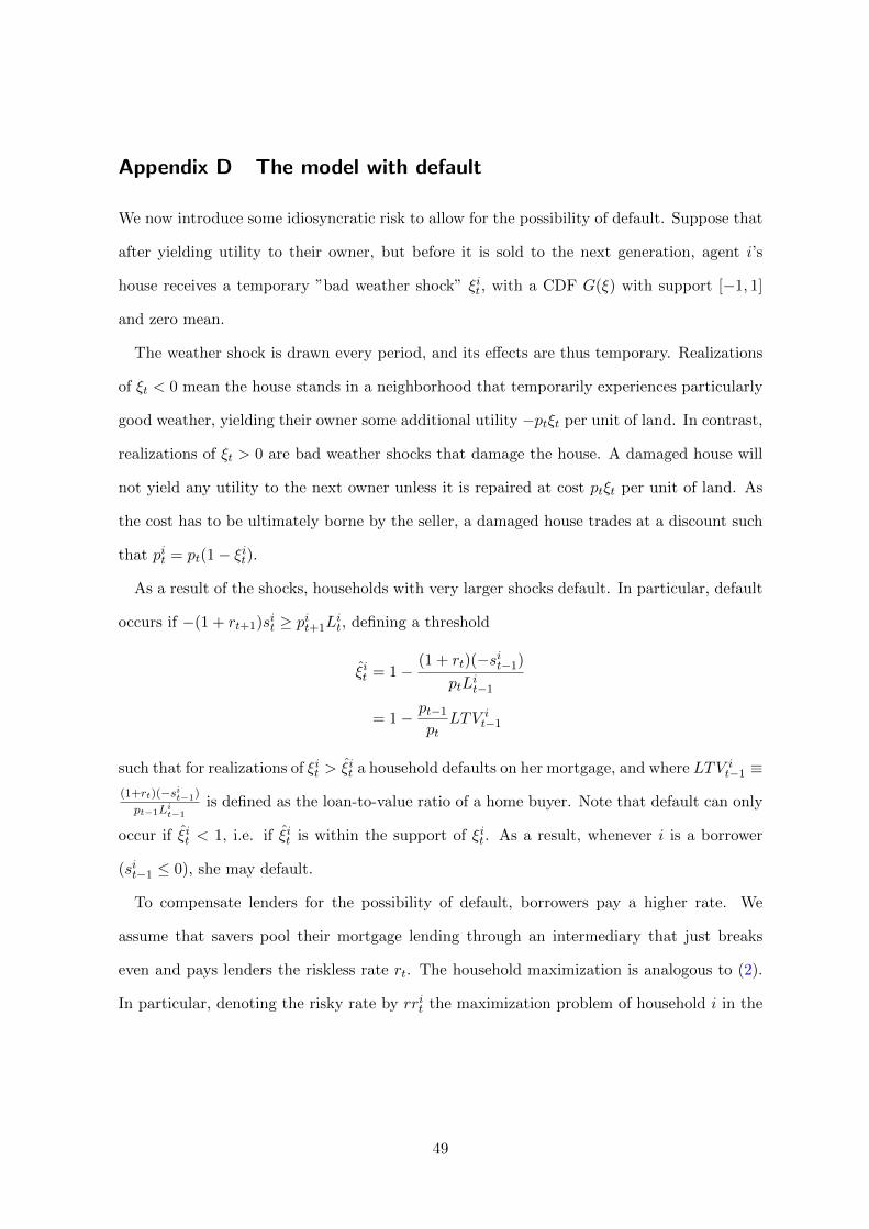
Appendix D The model with default

We now introduce some idiosyncratic risk to allow for the possibility of default. Suppose that

after yielding utility to their owner, but before it is sold to the next generation, agent i’s

house receives a temporary ”bad weather shock” ξit, with a CDF G(ξ) with support [−1, 1]

and zero mean.

The weather shock is drawn every period, and its effects are thus temporary. Realizations

of ξt < 0 mean the house stands in a neighborhood that temporarily experiences particularly

good weather, yielding their owner some additional utility −ptξt per unit of land. In contrast,

realizations of ξt > 0 are bad weather shocks that damage the house. A damaged house will

not yield any utility to the next owner unless it is repaired at cost ptξt per unit of land. As

the cost has to be ultimately borne by the seller, a damaged house trades at a discount such

that pit = pt(1− ξit).

As a result of the shocks, households with very larger shocks default. In particular, default

occurs if −(1 + rt+1)sit ≥ pit+1Lit, defining a threshold

ξit = 1−(1 + rt)(−sit−1)

ptLit−1

= 1− pt−1

ptLTV i

t−1

such that for realizations of ξit > ξit a household defaults on her mortgage, and where LTV it−1 ≡

(1+rt)(−sit−1)

pt−1Lit−1is defined as the loan-to-value ratio of a home buyer. Note that default can only

occur if ξit < 1, i.e. if ξit is within the support of ξit. As a result, whenever i is a borrower

(sit−1 ≤ 0), she may default.

To compensate lenders for the possibility of default, borrowers pay a higher rate. We

assume that savers pool their mortgage lending through an intermediary that just breaks

even and pays lenders the riskless rate rt. The household maximization is analogous to (2).

In particular, denoting the risky rate by rrit the maximization problem of household i in the

49

model with default becomes

maxcit+1,L

it,sit

EtU(cit+1, Lit) = Etcit+1 + v(Lit)

s.t. sit ≤ yit − ptLit

cit+1 ≤ max{yit+1 + pt+1(1 + ξit+1L

it + (1 + rrit+1)sit, 0

}cit+1, L

it ≥ 0

where the max-function in the t+ 1 budget constraint reflects that households are protected

by limited liability. The probability of default is [1 − G(ξit)], so that expected consumption

at t+ 1 can be written as

Etct+1 = G(ξit+1){pt+1(1 + Et[ξit+1|ξit+1 ≤ ξit+1])Lit + (1 + rrit+1)sit

}Now, the break even condition for the intermediary on borrower i is

−(1 + rt+1)sit = −G(ξit+1)(1 + rrit)sit + (1−G(ξit))pt+1(1 + Et[ξit+1|ξit+1 > ξit+1])Lit.

Plugging this condition into Etct+1 the objective function can be written as follows

EtU(cit+1, Lit) = yit+1 + pt+1L

it + (1 + rt+1)(yit − ptLit) + v(Lit)

The household problem boils down to choosing Lit to maximize EtU(cit+1, Lit). Differentiating

w.r.t Lit results in the first order condition and thus demand for land (??). It follows that

the allocation in the model with default is equivalent to the model without default. However,

now households with ξit > ξit default.

50