
Sectoral Imbalances and Long Run Crises* - Columbia ... · Sectoral Imbalances and Long Run Crises*...
48
1 | Page Greenwald etal 7 Sectoral Imbalances and Long Run Crises* Domenico Delli Gatti Università Cattolica, Italy Mauro Gallegati Università Politecnica delle Marche, Italy Bruce C. Greenwald Columbia University, USA Alberto Russo Università Politecnica delle Marche, Italy Joseph E. Stiglitz Columbia University, USA Abstract In this paper we propose an interpretation of the current Global Financial Crisis that emphasizes sectoral dislocation following localized technical change in the presence of barriers to labor mobility. This tale is reminiscent of the Great Depression. In the 1930s, technical change was localized in agriculture, where wages fell because of the costs of moving out of agriculture for unemployed workers. Shrinking wages in agriculture reverberated in the other sectors, causing a large depression. Now, it is manufacturing that plays the role of epicenter of technical change. Falling wages in manufacturing yield a lack of demand for goods produced in the rest of the economy, especially the service sector. This may be the underlying cause of the long-lasting slump and the painfully slow recovery. JEL Code numbers: G01, H12, J24, J61, O13, O14, O30, Q02 Key words: Crisis; Sector Imbalances; Productivity *Revised version of paper presented to the International Economic Association meetings, Beijing, July 8, 2011. Research assistance from Laurence Wilse-Samson and Eamon Kircher-Allen is gratefully acknowledged
Transcript of Sectoral Imbalances and Long Run Crises* - Columbia ... · Sectoral Imbalances and Long Run Crises*...
1 | P a g e G r e e n w a l d e t a l
7
Sectoral Imbalances and Long Run Crises*
Domenico Delli Gatti
Università Cattolica, Italy
Mauro Gallegati
Università Politecnica delle Marche, Italy
Bruce C. Greenwald
Columbia University, USA
Alberto Russo
Università Politecnica delle Marche, Italy
Joseph E. Stiglitz
Columbia University, USA
Abstract
In this paper we propose an interpretation of the current Global Financial Crisis that
emphasizes sectoral dislocation following localized technical change in the presence of barriers
to labor mobility. This tale is reminiscent of the Great Depression. In the 1930s, technical
change was localized in agriculture, where wages fell because of the costs of moving out of
agriculture for unemployed workers. Shrinking wages in agriculture reverberated in the other
sectors, causing a large depression. Now, it is manufacturing that plays the role of epicenter of
technical change. Falling wages in manufacturing yield a lack of demand for goods produced in
the rest of the economy, especially the service sector. This may be the underlying cause of the
long-lasting slump and the painfully slow recovery.
JEL Code numbers: G01, H12, J24, J61, O13, O14, O30, Q02
Key words: Crisis; Sector Imbalances; Productivity
*Revised version of paper presented to the International Economic Association meetings, Beijing, July 8,
2011. Research assistance from Laurence Wilse-Samson and Eamon Kircher-Allen is gratefully
acknowledged
2 | P a g e G r e e n w a l d e t a l
There has been a widespread presumption that the current economic crisis is a financial crisis, .
caused by the bursting of a credit bubble. Unjustified optimism about asset prices and associated risks
(primarily in housing but also in financial industry equities and even in equities generally),
accommodated by lax regulation, careless private lending and loose monetary policies led to
unsustainable levels of household and financial sector leverage. The inevitable collapse of the underlying
asset prices then caused widespread bankruptcies, foreclosures and impaired balance sheets among
households, firms and financial institutions. Combined with consequent large increases in the
incremental risks of lending and investing, these balance sheet effects induced large declines in
household spending, firm output and investment, and bank lending.1
This perspective has contributed to an understanding of what should be done, and the
economy's prospects. Consequently, U.S. government efforts to revitalize the economy focused on
pumping enormous sums into the banks. Now, more than four years since the beginning of the
recession, and more than three years since the enactment of TARP, the economy is not back to health,
and will likely not return to full employment for years to come.
1 Asymmetric information concerns have ruled out many natural financial market recapitalizations, like extensive
new equity issues. Some recapitalization was provided directly through government (TARP), but as we note later, most of the recapitalization was through retained earnings. The underlying theory, with its implications for banks, was set out several years before the crisis in Greenwald-Stiglitz (1993b, 2003) based on their work in the 1980s and early 1990s (see Greenwald and Stiglitz, 2003, for complete list), resting on micro-foundations provided by, for instance, Greenwald, Stiglitz, and Weiss (1984) and Majluf and Myers (1984). See also Bernanke, Gertler and Gilchrist(1999) on the working of the financial accelerator in an asymmetric information framework. For surveys, refer to Stiglitz (1988, 2011), Greenwald and Stiglitz (1993a). Many models focusing on balance sheet effects of financial disruption look not just at the financial sector (see, e.g. Greenwald and Stiglitz, 1993b; Adrian and Shin, 2008; and Shiller, 2008), though disruptions in the financial sector have particularly large systemic effects, and especially after the repeal of deposit rate restrictions, are particularly slow in reversing (Greenwald and Stiglitz, 2003). Household and company balance sheets are restored only slowly over time through accumulated savings and debt reductions associated with graduate declines in real asset holdings by means of inventory liquidations and gross investments levels below depreciation. The process has obvious adverse short run macroeconomic consequences.
3 | P a g e G r e e n w a l d e t a l
This paper provides an explanation for the depth and duration of the current downturn, in
contrast to other post-War recessions.2 Our assessment of the evidence suggests to us that the
underlying cause of the current crisis lies in real economic imbalances, exacerbated by financial crises to
which they gave rise (or hidden, for a time, by bubbles which led to unsustainable levels of
consumption). We argue that the structural transformation of the global economy from a manufacturing
economy to a service sector economy, necessitated, in a sense, by the impressive growth in
manufacturing productivity, is the real underlying cause of current problems in US and Europe. The
consequent adjustments have been exacerbated by globalization—the dramatic changes in comparative
advantages among countries of the world. But even had these not occurred, the increase in productivity
in manufacturing—at 6% or more per year, far outpacing growth in demand—would have meant a
decline in global manufacturing employment.3
While productivity gains are presumptively good for the economy, they are not unambiguously
so. There are losers and winners, and even if the winners could compensate the losers they seldom do.
But this paper is not concerned about the social consequences of these distributive impacts, but rather
with their macroeconomic consequences. Namely: In the absence of free migration, workers can
become trapped in the sector with rapidly increasing productivity. Especially if the elasticity of demand
for their output is limited, declining incomes in that sector translate into declining demands for goods in
2 There are other parts of the explanation that we cannot pursue here. For instance, countries, such as China, that
instituted strong Keynesian policies counteracted the decrease in global trade. Their policies were, at the same time, structural policies, sensitive to the changed composition of demand. 3 Indeed, Greenwald and Kahn (2008) estimate that between 1980 and 1991, a period of significant manufacturing
job loss, 85% of the decline in manufacturing employment was due to productivity growth, and only 15% was due to increased imports. While more recently, globalization has played a more important role, still, over the longer period from 1991 to 2007, two-thirds of the decline in manufacturing employment was due to productivity growth and only one-third to imports—the growth in China notwithstanding. If manufacturing productivity grows at 6%, even if the global economy grows at the impressive rate that it has been recently, say 4.5%, and manufacturing demands grows roughly commensurately, then global employment in manufacturing will decline. Globalization means that there is a global fight over where remaining jobs will be located, i.e. who has to make the largest adjustments.

4 | P a g e G r e e n w a l d e t a l
other sectors, with ambiguous welfare effects in other sectors4. Indeed, if there are efficiency wage
effects in the other sector(s), productivity shocks in one sector can give rise to unemployment in other
sectors, and be welfare-decreasing.
This paper thus illuminates the potential role of structural factors in crises, and highlights the
interactions between cyclical factors and structural factors. It distinguishes between “normal” business
cycles (typically generated by inventory fluctuations or by central banks stepping too hard on the brakes
in their inflation-fighting zeal5) and extended downturns. In the former, informational imperfections
giving rise to financial constraints amplify economic shocks6 . The latter are attributed to the collapse of
a major, often geographically isolated sector of the economy, though in these cases too financial
constraints amplify the consequences.7 8 The former are usually self-correcting and relatively short-lived.
The latter are long-lived and call for explicit government intervention.
4 Ambiguous because declining agricultural prices enhances urban worker welfare. Real wages measured in
manufactured goods may decline while real wages in agricultural goods may increase. This in fact happened in the Great Depression. In that case, urban real (consumption) wages, using the CPI, actually rose while manufacturing real product wages fell. But the appropriate model for describing what happened is one that incorporates unemployment, reflected in the efficiency wage model of section IV. (See Greenwald and Stiglitz, 1988). 5 The 1991-1992 recession is often related to the banking crisis that preceded it (see Stiglitz, 2003, Greenwald and
Stiglitz, 2003), and the 2001 downturn is generally related to the breaking of the tech bubble. But in both cases, as now, the bubbles that preceded these crises can be related to underlying problems in the real sector. 6 See, for instance, Greenwald and Stiglitz (1993b, 2003), Bernanke, Gertler and Gilchrist (1999 ), Korinek (2011)
or Stiglitz (2011). For surveys, see Stiglitz (1988) or Greenwald and Stiglitz (1993b). As Greenwald and Stiglitz (1993b) point out, these financial constraints not only can explain amplification (why small shocks can have large effects), but persistence, including why recoveries are so slow. These results stand in marked contrast to Real Business Cycle Models (RBC) without financial constraints, where the fluctuations simply reflect random real shocks to the economy. Indeed, in the absence of financial constraints, there are a number of “buffers,” like inventories, the effect of which is to dampen the impact of any real shock to the economy. 7 We should emphasize that there may be other real factors contributing to the insufficiency of aggregate demand.
In particular, the period before this crisis, as the period before the Great Depression, was marked by large increases in inequality. (Atkinson, Piketty, and Saez, 2011; United Nations, 2009; Rajan, 2010). With the marginal propensity to consume of high income households being less than that of low income households, such a redistribution would be expected to reduce aggregate demand. The necessary adjustments of factor and goods prices to restore a full employment general equilibrium may have been large, and evidently did not occur. Again, the financial sector played a role in forestalling the impacts: lower income individuals were able to continue to consume as if their incomes were not stagnating by borrowing.
One other real factor may have played a major role in this crisis: high oil prices redistributed income from the US and Europe and America to the oil producing countries, whose propensity to consume may be circumscribed by the recognition that given the high volatility of oil prices and the risks of Dutch disease problems, oil producers should set aside large fractions of their revenues.
5 | P a g e G r e e n w a l d e t a l
In the Great Depression, the collapsing sector was agriculture.9 Today, the sector in decline is
manufacturing. Increase in manufacturing productivity at a rate in excess of the rate of increase in
demand leads naturally to steadily declining manufacturing employment and income. Yet workers
continue to be trapped in the manufacturing economies both nationally, in countries like Japan, and
regionally, in U.S. states like Michigan.
The paper is organized into seven parts. The first describes in greater detail the evidence that
this crisis was not purely or fundamentally a financial one. The second provides a motivation for the
paper in terms of the Great Depression—arguing that just such a structural change, from agriculture to
manufacturing, was the real cause underlying the Great Depression. The third analyzes the
macroeconomics of a productivity increase in one sector in a simple model of an economy with free
migration among sectors. We structure the model in such a way that not only is GDP increased, but
everyone benefits. The fourth section describes what happen when the conditions necessary to support
migration no longer hold and workers are trapped in the high productivity but "dying" sector—dying
because it no longer generates jobs or because incomes are falling. The fourth section shows that the
problems are exacerbated if wages in the urban (manufacturing) sector are rigid, e.g. because of
efficiency wage consideration. The sixth then analyzes three policy responses—fiscal policies, wage
policies, and migration policies. The seventh then expands the analysis from a closed economy to an
open economy. It shows that in this situation of "blocked" migration, some individual nations/regions in
a global economy can (temporarily) improve their situation by, for instance, manipulating exchange
rates, with, however, adverse consequences for others. A brief conclusion follows.
Still another factor contributing to the global crisis was the large build-up of reserves by emerging
countries (motivated sometimes by a precautionary demand for savings, sometimes by the pursuit of export led development strategies in the presence of constraints on industrial policies). (See Greenwald and Stiglitz, 2010a and 2010b.) Whatever the motivation, the increase in reserves subtracted from global aggregate demand. 8 There is another major deficiency in RBC and related models. In those models, the shock to the economy is
exogenous and it is modeled by a simple stochastic process. In reality, the most important disturbances are endogenous and episodic—whether they are bubbles or the structural transformations upon which we focus here. 9 As well as, perhaps, marginal manufacturing using techniques pre-dating the rollout of electrification and mass
production.
6 | P a g e G r e e n w a l d e t a l
I. An Incomplete Explanation for the Crisis and the Great Recession
Understanding the nature of the crisis—and why the economy has remained weak—is essential
not only for interpreting the events of the past few years, but for ascertaining prospects and assessing
policies going forward.
Initial assessments and policy interventions have focused on the role of the leveraged financial
sector, and the subprime spark. Furthermore, recoveries from financial crises, it is said, are slow,
partially because bank and firm balance sheets recover only slowly.10 Financial crises are typically
associated with the destruction of information, e.g. about who is creditworthy, as banks are pushed into
bankruptcy. (Greenwald and Stiglitz, 2003). In contrast to the policies pushed by the IMF and the US
Treasury in Indonesia and elsewhere during the East Asia crisis, we congratulate ourselves in having
preserved these institutions, admittedly at some risk of moral hazard going forward. But there is still
the slow process of rebuilding bank balance sheets.
But, the failure of the strategies undertaken to end the crisis hints at the incompleteness of the
diagnosis that informed them. Since the crisis was deemed to be a financial one, lawmakers and central
bankers crafted policy on the assumption that if the financial system were repaired, the economy would
return to health. This gave a sense of priorities to government. It provided justification for the bank
bailout, and TARP; political leaders supporting this highly unpopular bailout could feel virtuous because
they put the well-being of the economy over pursuing short-term political advantage. With a quick
repair of the financial system in the offing, only a short-term stimulus was required to tide the economy
over.
The weaknesses in the economy have, however, turned out to be more persistent than this
diagnosis would have suggested; the Fed has (as of early 2012) committed itself to leaving interest rates
at near zero through the end of 2014. Though there are still many concerns with the financial system 10
See, e.g. Reinhart and Rogoff (2009). The theory is set forth, e.g. in Greenwald and Stiglitz (1993b)
7 | P a g e G r e e n w a l d e t a l
(lack of transparency, inadequate SME lending, weaknesses in many local and regional banks), it is not
apparent that finance is holding the economy back. (Of course, in any crisis, the real and financial
sectors are intertwined: any real crisis, lasting long enough, will have consequences for the financial
sector; and the subsequent weaknesses in the financial sector will have real consequences. That is why
ascertaining causality is always going to be difficult.11 )
If the financial sector were the cause of the economy’s current problems, it should be reflected
most strongly in investment. But business investment in the United States, as a percentage of GDP, is
not particularly low—certainly not in a way that would be suggested if the availability of funds were the
binding constraint. Indeed, large businesses are reportedly awash with cash.12
Of course, investment in real estate is constrained—less than half the pre-crisis level, but, with
real estate prices down 30 to 40%, that would presumably be the case even with perfectly functioning
financial markets. Indeed, the excessive investment in real estate was really a symptom of a
11
Financial sector problems arise both directly, as a result of a weak economy, and indirectly, as a result of government responses to the fear of a weak economy. Governments may respond to what otherwise would be a weak economy by lowering interest rates and weakening regulation, or undertaking other policies that help create future financial crises. Arguably, this was the case in the U.S. 12
Private non-residential fixed investment as a percentage of GDP was around 10.0% in the second quarter of 2011, while the historical post-war average is 10.7% (though, we note that GDP has fallen below trend). Equipment and software investment by firms in real terms was about 8.2 percent of GDP in early 2011 compared to a high of 8.4 percent in 2007 and 6.6 percent at the peak of the crisis in the fourth quarter of 2008. These investments, being difficult to collateralize, are the first to suffer when bank lending is restricted. Their relatively high level suggests that a shortage of bank lending has not had a significant dampening effect on business investment. Business investment in structures has fallen sharply but this appears to be due more to the overhang of empty buildings from the earlier boom than to limitations on bank lending. The level of commercial and industrial lending for small domestic banks rose in the second quarter of 2011 to 2
nd quarter 2007 levels, after a prolonged period of
being far lower. (Seasonally adjusted commercial and industrial loans at all commercial banks were $1.293 trillion on August 1, 2011, and $1.293 trillion on July 1, 2007, according to figures from the St. Louis Fed. Available at http://research.stlouisfed.org/fred2/categories/32389, accessed January 24, 2011). The trend toward industrial firms holding more cash is not new. Bates, Kahle and Stultz (2009) document between 1980 and 2006 a doubling in the average cash-to-assets ratio for US industrial firms, such that “at the end of the sample period, the average firm can retire all debt obligations with its cash holdings.” They find (p. 2018) that the “main reasons for the increase in the cash ratio are that inventories have fallen, cash flow risk for firms has increased, capital expenditures have fallen, and R&D expenditures have increased” (where cash flow risk is measured as the standard deviation of industry cash flow to assets). It may be that the post-crisis build-up in cash reflects increased uncertainty and the consequences of the extreme credit conditions of 2008, which many businesses fear may occur again.
8 | P a g e G r e e n w a l d e t a l
dysfunctional financial market; one can hardly complain about a market that finally begins to show some
sense of "rationality" after a prolonged period of excess.
There is another reason for suspecting that finance is not the major constraint in the economy’s
recovery—and therefore not the only explanation for its weakness. If the financial sector were really
broken, real lending rates would presumably be very high. With inflation around 2%, real T-bill rates
are now markedly negative, and even prime lending rates are very low (adjusted for inflation, a little
over 1%).13 This is in marked contrast to the Great Depression, in which prices were falling at 10% a
year, so real interest rates were, in fact, very high. Indeed, the low (negative) real interest rates raise
questions about conventional monetary theory and policy, which focus on real interest rates. Some
economists have even suggested that the limitation of monetary policy in restoring the economy is the
"zero lower bound," and some (such as Krugman14) have made reference to a (Keynesian) "liquidity
trap.” With real interest rates already negative, it is hard to believe that high interest rates are keeping
the economy from recovering, and the data on investment cited earlier is consistent with this
perspective. recession, where, It is hard to argue that with these low real interest rates, finance is the
critical constraint.15
Another aspect of the conventional wisdom is that if the economy is to recover, households
must deleverage. The fact that the process of deleveraging is so slow—in the absence of some process
of debt restructuring—adds pessimism about the economy's prospect. There is no doubt that the fact
that nearly one out of four Americans with a mortgage is underwater (an aggregate gap between what is 13
Inflationary expectations, as reflected by TIPS, are also low. The average spread between TIPS and 10-year treasuries (a good measure of expected inflation) was about 2 percent from 2010 through the summer of 2011. The CPI increase between August 2010 and August 2011 (excluding food and energy) was also 2 percent (although the overall index including food and energy increased by 3.6 percent). Data from St Louis Fed, available at http://research.stlouisfed.org/fred2/series/CPILFESL and http://research.stlouisfed.org/fred2/series/CPIAUCSL?cid=9. 14
Krugman (2009) and Eggertsson and Krugman (2010). 15
More accurately, it is hard to argue for this within the conventional models, in which credit rationing does not exist. Stiglitz and Weiss [1981] explain why there may be credit rationing, and Greenwald, Stiglitz and Weiss (1984) explain why the extent of credit rationing may vary over the business cycle. But as we noted, the level of investment in equipment and software and the magnitude of cash holdings by large firms suggests that by mid 2011 finance was not the major constraint on recovery.
9 | P a g e G r e e n w a l d e t a l
owed and the value of the underlying property estimated at some $700 billion16) causes anxiety and
considerable misery among a substantial fraction of American citizens, and one can argue that it was
unconscionable—and politically unwise—to ignore this, especially as money was shoveled to the big
banks. Others hope that, somehow, even with the slow pace of deleveraging, the American consumer
will return; they look carefully at the monthly sales data to see some indication that that might be the
case.
A closer look at the data, however, suggests that deleveraging, as desirable as it might be from a
welfare point of view, is not going to lead to significant increases in consumption—certainly not the
basis of a strong recovery.
Sustaining near full-employment in countries like the United States prior to the crisis of 2008
seems to have depended on extraordinarily profligate consumer behavior. Under ordinary
circumstances, a near zero savings rate like that of U.S. households in the mid-2000s should have
generated significant inflationary pressure. But in spite of the absence of inflationary pressures, the low
savings rate was clearly unsustainable. High income households, with roughly 40 percent of permanent
income, typically save 15 percent or more of their incomes17. By themselves, they account for a 6
percent savings rate out of total income: 15 percent of 40 percent. An overall zero savings rate,
therefore, required that middle and lower income households with 60 percent of permanent income
dis-save at a rate of 6 percent of total income per year. This, in turn, meant that these households had
to spend 110 percent of their incomes every year: -10 percent savings times 60 percent for -6 percent of
total income. The return to a zero savings rate by middle and lower income households in the wake of
the 2008 financial crisis, which eliminated their continuing ability to borrow, led to an increase in the
16
Moody’s estimates that some 14 million homeowners are in positions of negative equity, “half by more than 30% … (and) the average underwater homeowner’s debt exceeds market value by nearly $50,000” (Zandi 2011, p. 2). 17
Dynan, Skinner, and Zeldes (2004, pp 399-400) find savings rates varying from zero for the lowest quintile of the income distribution to in excess of 25 percent for the top.
10 | P a g e G r e e n w a l d e t a l
overall savings rate to roughly 6 percent.18 The consequent decline in consumption demand appears to
have been the proximate cause of the recession. (Housing demand began to decline in early 2006.)
Continued prosperity pre-crisis seems to have depended on continued bubble-driven consumption. If a
return to “normal” savings levels was inevitable, then the financial crisis affected the timing rather than
existence of a severe recession.19 By the same token, “fixing” the financial system, or even deleveraging,
is not likely to have a substantial, sustained effect on aggregate consumption, and therefore on
aggregate demand. The savings of the bottom 80% are not likely again to be negative, and those of the
upper 20%, are not likely to fall much below 15%.20 21
Looking at this and other crises around the world throws further doubt on the hypothesis that
this is centrally a financial sector crisis. First, the severity of the downturn has generally been unrelated
across countries to the financial origins of the crisis. The United States and the United Kingdom, both
countries with outsized financial sectors that failed spectacularly in the wake of widespread financial
misbehavior, suffered relatively less severe output declines than other nations with sounder financial
systems and no notable failures of financial institutions. Finland, Japan, Germany, Denmark and Italy all
suffered larger declines in GDP than the United States and the United Kingdom. In other countries—
18
Personal savings rates were around 5% in 2009, before rising towards 6% in 2010. At the end of 2011, rates dropped back down to 3.5% , around what they were in 2004. 19
The analysis of this paper does not deny the importance of the failings of the financial sector in determining not only the timing of the crisis, but also the depth and duration of the downturn. The legacy of excess investments in real estate and of excessive indebtedness by households is playing a role, just as— we argue below—the build-up of “forced savings” during World War II helped not just to prevent the US from sliding back into recession or worse, but to propel the country into a new prosperity. 20
Deleveraging could have one important effect on aggregate demand: lower expenditures servicing debt would leave more money to spend on real goods—illustrating another way in which the excessive financialization of the economy may have contributed to its weaknesses. But the data suggests that this effect is likely, at most, to be small—perhaps because of the innovativeness of the financial sector in finding new ways of extracting money from consumers, partly because some of the deleveraging is taking the form of home foreclosures, forcing individuals into rental properties, which over the longer run may actually reduce what can be spent on other goods and services. Non-consumption household outlays, which include household interest payments fell from 3.94% of total outlays at the peak of the borrowing boom in 2007 to 3.45% at the end of 2010. The resulting increase in funds available for consumption was less than .5 percent, and this includes the impact of lower household interest rates as well as deleveraging. 21
Once the deleveraging process is completed, the rate of growth of consumption might be restored to a more normal level. But full economic recovery, with a restoration of full employment, would require still more rapid growth.
11 | P a g e G r e e n w a l d e t a l
Spain, Ireland, Greece and Portugal—financial difficulties and banking insolvencies appeared late in the
crises following severe real economic contractions. In these cases, financial crises appear to have been
the consequence rather than the cause of the recession, though weak financial systems are more likely
to be damaged by a “real” economic downturn, and the consequent financial crisis may serve to prolong
the downturn.22
Moreover, for all the talk of a “great moderation,” the period since 1980 has been characterized
by severe persistent crises outside the United States23 and, in many quarters, slow growth.24 Crises, in
particular, have become far more frequent and more severe. What is striking is that this was in a period
where economists claimed we knew more about economic management, and more countries followed
the precepts advocated by economists. One explanation is that what was "learned" was wrong, and the
policy advice was a move in the wrong direction. Another explanation (not necessarily mutually
exclusive) was that there were real changes which lead even well-managed economies into crises, or at
least increased the difficulties of economic management.
22
This data is only meant to be suggestive, because many factors contributed to the depth of the downturn and the speed of recovery (and there are alternative measures of the depth of the downturn—Germany had a larger downturn in output, but a smaller downturn in employment). Some countries (such as China) took strong actions to offset the downward pressures. Still, these experiences suggest that it is structural factors (the composition of output and trade dependence), as much as weaknesses in the financial sector, that determined the depth of the downturn. With the precipitous fall in trade, especially in manufactured goods, countries that were more dependent on exports of manufactured goods suffered more, ceteris paribus. To be sure, with weak banking systems, precipitous declines in GDP can translate into financial sector problems, making the challenge of recovery greater. The evolution of the crisis has also thrown doubt on other shibboleths. A central contention of some central bankers (and many strands of macroeconomics) has been that it is wage rigidities which give rise to extended periods of unemployment. Yet, in this crisis, the United States, supposedly the advanced industrial country with the most flexible labor market, has been plagued with higher and more persistent unemployment (especially relative to the drop in GDP) than, say, Germany. This is consistent with both theoretical work (surveyed in Greenwald and Stiglitz, 1993a) that argues against the hypothesis that it is wage and price rigidities that are primarily responsible for the magnitude of employment and output fluctuations (on the contrary, fluctuations may be greater with more flexible wages and prices) and with the confirming empirical studies (Easterly, Islam, and Stiglitz, 2001a and 2001b). 23
Even the United States had one costly costly, the S & L crisis of the 1980s, and would have had more had the government not engineered (through the IMF) bailouts, e.g. as a result of the Latin American debt crisis. 24
Employing the definitions of Reinhart and Rogoff (2009), the proportion of countries experiencing new external debt crises reached as high as 40% in the mid-1980s, and the proportion of countries experiencing banking crises reached 30% in the late 1990s. These were the highest since the Second World War and represented a precipitous increase since the moderate period between 1945 and 1980 (Reinhart and Rogoff 2009, p. 74).
12 | P a g e G r e e n w a l d e t a l
While in some of the crises, bubble-like behavior played a relatively minor role, Japan in the
early 1990s did suffer from the collapse of a spectacular financial bubble and a badly impaired banking
system. But by 2000, these problems were in the past; yet stagnant economic growth continued. The
generally disappointing rate of recovery from the crisis in many countries besides the US (with the
important exception of the emerging markets) despite the marked improvement in the financial sectors
in these countries25, suggests that the Japanese experience may not be an isolated one.
The real changes in the economy that we believe are at the core of the problem of economic
adjustment are those caused by the enormous increase in productivity in manufacturing. The issue has
to be looked at, as we have noted, from a global perspective. While the increase in manufacturing
productivity in excess of the increase in demand for manufactured goods will mean that the global
manufacturing employment will decrease, there are, at the same time, shifting comparative advantages.
26 Countries that both have a large manufacturing sector and are losing their comparative advantage
will face the largest structural transformations—and thus may be the countries (ceteris paribus) most
affected by the crisis.
Not surprisingly, because the cause of this downturn is different from that of other more recent
recessions, it is plausible that the policy response might have to be different. There should be structural
policies to facilitate the movement of labor that is "trapped" in a dying sector, and that requires
understanding the economic forces that impede mobility. But even though structural policies are part
of the solution, traditional Keynesian policies play a role. The corrective intervention that brought about
25
There have been extensive recapitalizations, both through the issue of new shares and (sometimes forced) retention of high earnings (facilitated by the low interest rates at which the banks can get access to funds). Still, critics argue that what has been done is not enough, that banks continue with highly risky activities, that their lack of transparency makes it difficult to judge the adequacy of their capital, and that, as a result, weaknesses in the financial sector continue to plague the economy. The lack of confidence in the financial sector is manifested by the high volatility of bank share prices. Still, the most direct consequence of the weaknesses in the financial sector should be on the level of investment, and, apart possibly for the availability of finance to SME’s, this does not seem to be impaired by weaknesses in the financial sector. 26
Far more important than relative resource endowments is knowledge, so that what matters is dynamic comparative advantage, which is endogenous, and which can change markedly over time (Greenwald and Stiglitz, 2006 and 2012).

13 | P a g e G r e e n w a l d e t a l
the end of the Great Depression was World War II—but not as it is generally interpreted. As we explain,
the policies were both Keynesian (a massive economic stimulus) and structural. Today, correcting this
situation will require a focused effort in managing the transition of workers on a global basis out of
manufacturing into services with an impact comparable to that of World War II in moving workers off
the farm. Our analysis, which shows that well-designed Keynesian responses may be appropriate even
when there is a structural aspect to the underlying crisis, stands in marked contrast to those who now
claim that most of the remaining unemployment is structural—there is a new "normal" to which we
must now accommodate ourselves—and therefore policies designed to stimulate the economy may not
only be useless, they may be counterproductive.
II. The Great Depression as a "Model" for the Current Downturn
The depth and duration of the present crisis is outside the normal range of post-World-War-II
experience.27 Not surprisingly, then, there is renewed interest in the previous episode of a long
downturn, the Great Depression (Temin, 2010).28
Our thinking has also been greatly shaped by reflections on the Great Depression. Many
attribute that economic downturn (like this one) to the financial sector—a stock market bubble,
27
As this paper goes to press, it is far from clear that the crisis is over, despite fiscal and monetary interventions that have also been without precedent in the post-War era (and even the pre-War period). Most projections suggest that it will be years before unemployment returns to "normal" levels. 28
There is also a resurgence of interest in the ways in which deep downturns differ from ordinary downturns. See Stiglitz (2011). Interestingly, there is no consensus about the causes of the Great Depression, including the relative role of monetary versus real forces. See, for instance, Temin's Lionel Robbins Lecture (1991). The explanation we provide here focuses on the source of the underlying disturbance to the economy, and one of the impediments to the economy's adjustment to this disturbance. Greenwald and Stiglitz (1993b, 2003) discuss other factors that contribute to the amplification and persistence of shocks, including financial market constraints and imperfections. This analysis does not rule out that flawed monetary and regulatory policies and asset price bubbles might have contributed to the depth and duration of the Depression. As we argue below, however, increasing wage flexibility might have made matters worse (in contrast to much of standard New Keynesian analysis where the focus of attention is on nominal wage (or price) rigidities.) The analysis is also consistent with the hypothesis that asymmetries in adjustment speeds across sectors played an important role in the evolution of the crisis. See Stiglitz (1999).
14 | P a g e G r e e n w a l d e t a l
supported by excessive margin, which, when it broke, had large effects on balance sheets. Clearly, too,
the banking failures played an important role in the dynamics of the Great Depression. But was it not
possible that the stock market bubble itself was hiding underlying weaknesses and more fundamental
problems, just as the housing bubble did in the years before the Great Recession? Indeed, the global
banking crisis in 1931 appeared relatively late in the global decline. A country, like Canada, with no
significant banking issues, appears to have suffered as much in the Depression as countries that
experienced severe banking crises. The Depression, we believe, ultimately arose from real factors rather
than financial imbalances.29
In the case of the Great Depression, it is clear what the underlying real problem was: declining
prices and incomes in the agricultural sector.30 In the United States agricultural prices began to decline
precipitously in August 1929, well before the stock market crash in October of that year, and continued
to fall for years. It was to be another four years before banking failures reached their zenith, with the
enforced “bank holiday” in 1933.31
It is easy to infer both the causes and consequences of the decline in agricultural prices and
incomes. Long-term increases in global farm productivity coupled with increases in land under
cultivation had, since the second-half of the 19th century, led to long-term increases in farm output
above the rate of increase of farm demand and, thus, secularly declining farm prices. Harvest and
29
Reinhart and Rogoff (2009) claim to have identified the unusually prolonged consequences of business cycles associated with financial crises. But, they make no serious attempt to examine the original causes of these crises. To the extent that severe real imbalances that take a long time to resolve ultimately lead to financial crises more often than less severe ones, financial crises will be a symptom of severe real imbalances. In this case, they have merely discovered that severe imbalances are more prolonged than mild ones. 30
Contemporaneous work citing the importance of agriculture includes League of Nations (1931) and Timoshenko (1933). In a public lecture given in October 1931, Dennis Robertson ascribes the “primary cause” (original emphasis), as the ‘glut’ of capital goods and, in particular, “(i) the rapid application of science to agriculture […] leading […] leading to a decline in the total receipts even of [low-cost producers], (ii) the decline of the rate of growth of the population […] (iii) the durable nature of some new objects of consumption,” (Robertson 1956, p.72). 31
Initial banking distress was particularly acute in rural areas. Chandler (1970, p. 62) reports, “in the three years 1930-32, 5,096 banks failed in the United States, 3,448 of these […] were in places with populations below 2,500.”
15 | P a g e G r e e n w a l d e t a l
demand fluctuations32 meant that this trend was far from uniform and there were periods of high prices
and farm prosperity. But, by the late 1920s33, farm prices were in steady-decline, with consequent
effects on farm income.
Gross farm income in current dollars fell from $17.9 billion in 1919 to $13.9 billion in 1929 to
$6.4 billion in 1932—a decline of more than 50% in three years— before recovering to $11.4 billion in
1937.34
Given the size of the agricultural sector (farm population represented 30% of the total in 1920)
it is not surprising that a decline in that sector would have macro-economic consequences. These
declines represent losses that are a significant fraction of GDP. (The loss in gross farm income between
1929 and 1932 represented 13% of 1932 GDP.)
32
Combined with supply effects associated with expectations of future prices, the impact of financial constraints in limiting investment in agriculture, and speculative hoarding. 33
Chandler (1970) cites the 23m acres of farmland that became available from the replacement of draft animals by automobiles, trucks and tractors. He also notes as important (1970, p.55), “Continued advances in technology [which] were a major force tending to increase total farm output. These took many forms: improvements in methods of farm management, better adaptation of crops to soils, development of more efficient plants and animals, and so on.” 34
Net farm income after expenses fell from a peak of $9.6 billion in 1919 to $6.3 billion in 1929 to $1.9 billion in 1932. It recovered to $5.7 billion in 1937 and fell to $4.2 billion in 1938 where it remained through 1940. Net farm income deducts farm wages. Nominal GDP was: $84 billion in 1919, $103.1 billion in 1929, $58 billion in 1932, and $84.7 billion in 1937; while at 1958 prices it was, 146.4, 203.6, 144.2 and 203.2, respectively. Source: United States Bureau of the Census, 1975, Historical Statistics of the United States Colonial Times to 1970, pp. 483-4.
There are, of course, two possible reasons for the dramatic decline in income—a fall in prices or a fall in quantities. Our model is predicated on an increase in productivity which would have generated a decline in prices even in the absence of a recession/depression; but the recession/depression exacerbated the magnitude of the decline, as the model in the following section illustrates, but given the low income elasticity of food, the quantitative importance of this may be limited. Data for internationally traded goods (cotton, corn, and wheat) show dramatic declines in prices from 1929 to 1932. In some parts of the United States, these price declines were reinforced by quantity declines as a result of the environmental disaster (the dustbowl) (Hornbeck, 2011). However, in the aggregate, quantities actually increased. As detailed by Chandler (1970, p. 58), “In contrast to behavior in most other industries, real output in agriculture did not fall […] total farm output in 1931 and 1932 was slightly higher than in 1929. The most important reasons […] were the recognition by each individual farmer that he could not raise prices by reducing his output […]” Chandler concludes (1970, p. 59), “Thus, the entire decrease in the money incomes of farmers resulted from declines in the prices of farm products […] by 1932, prices received by farmers had fallen 56 percent below their levels in 1929, while prices paid by farmers had declined only 32 percent.” One might ask why, beside the fall in demand and the price inelasticity of demand, should there have been a decline in prices of this magnitude, given the limited rise in agricultural output. One explanation is that prior to 1929, farmers had been hoarding, in the anticipation that prices would rise, so that the flow of produce on the market was less than the output. Once storage capacity constraints are reached, the flow of produce must equal that of production; and if market participants anticipate that prices will not recover any time soon, or can no longer finance large stocks in storage, de-hoarding will occur, so that the flow of produce will exceed production.
16 | P a g e G r e e n w a l d e t a l
One would have anticipated that declines of this magnitude would have led to mass migration.
And in the 1920s, it did, with farm population as a percentage of the total falling from 29.9 to 24.8
percent of the total from 1920 to 1929. But remarkably, in the 1930s, migration was limited, with farm
population falling, proportionally, by just 1.4 percentage points in the 1930s (to 23.4 percent by 1940.)35
The explanation is easy: the effective push and pull were far weaker than the wage discrepancies would
have suggested. Farmers had almost all their capital invested in rural houses, farm equipment, land,
local structures, and related equipment. The sharp decline in the value of this capital coupled with the
simultaneous decline in farm income impaired the financial positions of farmers and their local lending
institutions. Thus, farmers could not afford to migrate to the cities. Moreover, with high urban
unemployment in the 1930s, the migrant's prospects were bleak.36 As a result of the inhibited
migration, the benefit that would have been enjoyed from higher farm productivity as a result of
reallocating labor was largely lost.
This loss of income to farmers itself led to weakening demand for urban goods, leading to lower
incomes and employment there, and this in turn led to declining demands for agricultural goods, in a
downward vicious circle. In short, we argue that the "shock" to the economy which led to the low level
equilibrium was a positive productivity shock in agricultural—combined with frictions that trapped
workers in the rural sector.
There is one obvious objection to this analysis: The fall in agricultural prices can be thought of
as purely redistributive: farmers lose, those in the urban sector gain.37 But there are several reasons
that the net effect on aggregate demand in the short run could be markedly negative. The resulting
decline in rural demand for industrial output would have outweighed any increase in urban demand as
35
In fact, between 1931 and 1934 there was net in-migration of around 700k (compared to, for example, net outmigration of 6.4m between 1942 and 1944). See Carter, et al. (2006). 36
The theory of migration from rural to urban sectors, taking account of the consequences of urban unemployment, and rural credit constraints, is well developed in the development literature. See, for instance, Harris and Todaro (1970) and Stiglitz (1969, 1974). 37
In an open economy, there is a net loss (if the country is a food exporter, like Argentina or the U.S.) or a net gain (if the country is a net food importer).
17 | P a g e G r e e n w a l d e t a l
long as the marginal propensity to increase consumption by urban households was lower than the
marginal propensity to reduce consumption by rural households. Several factors made such an outcome
likely. First, budget-constrained rural households would have been forced to reduce their consumption
of industrial goods sharply and immediately. Newly better-off industrial households would have had the
freedom to adjust more slowly to their higher real incomes. Secondly, if they were uncertain about the
permanence of the price changes (i.e. whether their permanent income had increased), they would not
have wanted to adjust their spending quickly. Thirdly, if the marginal propensity to consume declines
with income, the per dollar impact of declining incomes among already relatively poor rural households
would have been larger than the impact of rising incomes for richer urban households.38 Fourthly, the
failure of rural financial institutions and the impairment of rural assets would have greatly limited the
ability of borrowing to offset the effects on demand of declining rural incomes.39 The stimulating impact
of lower lending constraints on largely unconstrained urban households would have been far smaller.
(Consumers’ ability to borrow for purposes of consumption smoothing was limited, far more so than it
38
Hansen (1941, pp.232-234) derives numbers from the 1939 Consumer Expenditures in the United States indicating the propensity to consume for 1935-36. For income earners earning less than $500, consumption as a percent of income is found to be 149.4 percent, for those earning in excess of $20,000, this falls to 49.3 percent. Marriner Eccles (1951, p.76), appointed Chairman of the Federal Reserve by Roosevelt, framed the problem as “by taking purchasing power out of the hands of mass consumers, the savers denied to themselves the kind of effective demand for their products that would justify reinvestment of their capital accumulations in new plants. In consequence, as in a poker game where the chips are concentrated in fewer and fewer hands, the other fellows could stay in the game only by borrowing. When their credit ran out, the game stopped.” Attempting to explain his high, back-of-the-envelope estimated multipliers for the Depression period, Field (2011, p.240) observes, “[the] Depression reduced income, but it also reduced inequality, and this reduced saving both in the aggregate and as a share of GDP. Gross saving as a share of GDP was 18.6 percent of GDP in 1929, but fell to 5.6 percent in 1932. It recovered to 17.5 percent in 1937 and had risen to 23.5 percent in 1941.” 39
Between 1930 and 1932, 68% of bank failures were in rural areas --- where populations were below 2,500 people (Chandler, 1970, p. 62). Friedman and Schwartz describe the onset of the First Banking Crisis in October 1930 as beginning in the agricultural sector: "A contagion of fear spread among depositors, starting from the agricultural areas, which had experienced the heaviest impact of bank failures in the twenties" (Friedman and Schwartz 1963, p.308). Madsen (2001, p.328) makes similar points across countries --- “The declining real prices of agricultural products […] had adverse effects on consumption and investment. First, the marginal propensity to spend of those who lost income exceeded the marginal propensity to spend of those who experienced income gains. Second […] declining real prices of farmland […] increased the cost of borrowing for farmers, and thus adversely affected investment and […] consumption. Third, the declining ability of farmers to honor their debt obligation adversely affected the functioning of the banking sector […] For the United States […] William Arthur Lewis argues that the declining agricultural prices, the fall in real estate values, and the bankruptcy of farmers were the most important factors behind the bank failures.”
18 | P a g e G r e e n w a l d e t a l
was prior to this crisis.) Limitations in the ability of banks to lend to farmers is the one aspect in which
weaknesses in the financial sector contributed to the underlying macroeconomic weaknesses—and to
keeping workers trapped in the dying sector; but for most farmers, it was probably not the operative
constraint, for given the circumstances, even strong financial institutions would have been reluctant to
lend to farmers whose income was declining so rapidly.
In the formal model presented later, there is one further effect: the decline in prices leads to a
substitution away from manufactured goods. This strengthens the adverse impacts on the urban sector.
While the positive effect of the substitution effect partially offsets the direct negative effect of the
productivity shock on rural incomes, so long as the system is stable, it can only partially do so.
For all these reasons, the collapse of agriculture would have been expected to lead to a parallel
decline in overall urban industrial demand, and this is what happened.40 At the very least, incomes in the
industrial sector would have been expected to decline markedly, as labor demand fell. If wages were
flexible, there would have been large redistributions from labor to capital in the urban sector, with
further adverse effects on aggregate demand. But if wages were at all rigid, for instance, because of
efficiency wage considerations, then unemployment would increase markedly.
It is not surprising, given the magnitude of the negative shock from the agriculture sector, that
the limited increases in Federal spending during the New Deal (partially offset by decreases in state and
local spending) had limited effects.41 Moreover, Federal spending was variable, declining markedly in
1937.
40
For empirical data on the subject, see Bell (1940); Swanson and Williamson (1972). Note too that increased uncertainty of future income, as the crisis evolved, may have reinforced these effects, as even urban workers who retained their jobs and benefited from lower agricultural prices faced a risk of a job loss, with poor prospects of reemployment. The model below does not incorporate this effect, or one other, that may be playing a role in the current crisis: the resulting weaknesses in the urban labor market may lead to some lowering of real urban wages (even in the presence of efficiency wage concerns), and the resulting intra-sectoral redistribution may have an adverse effect on aggregate demand. 41
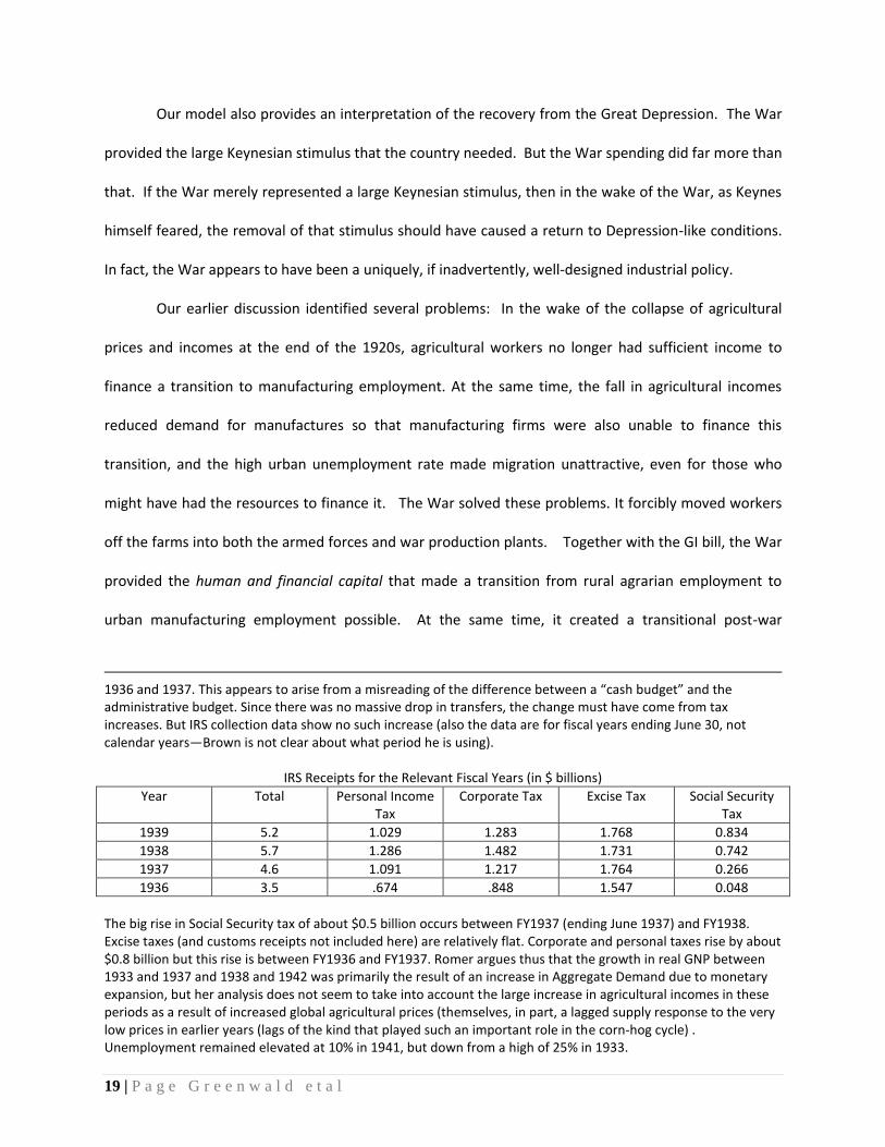
Romer (1992) finds almost no role for fiscal policy in the recovery from Great Depression between 1933 and 1942, “fundamentally due to the fact that the deviations of fiscal policy from normal were not large during the 1930s” (p.768). Cary Brown also shows an increase in net taxes (taxes minus transfers) of $2.9 billion between
19 | P a g e G r e e n w a l d e t a l
Our model also provides an interpretation of the recovery from the Great Depression. The War
provided the large Keynesian stimulus that the country needed. But the War spending did far more than
that. If the War merely represented a large Keynesian stimulus, then in the wake of the War, as Keynes
himself feared, the removal of that stimulus should have caused a return to Depression-like conditions.
In fact, the War appears to have been a uniquely, if inadvertently, well-designed industrial policy.
Our earlier discussion identified several problems: In the wake of the collapse of agricultural
prices and incomes at the end of the 1920s, agricultural workers no longer had sufficient income to
finance a transition to manufacturing employment. At the same time, the fall in agricultural incomes
reduced demand for manufactures so that manufacturing firms were also unable to finance this
transition, and the high urban unemployment rate made migration unattractive, even for those who
might have had the resources to finance it. The War solved these problems. It forcibly moved workers
off the farms into both the armed forces and war production plants. Together with the GI bill, the War
provided the human and financial capital that made a transition from rural agrarian employment to
urban manufacturing employment possible. At the same time, it created a transitional post-war
1936 and 1937. This appears to arise from a misreading of the difference between a “cash budget” and the administrative budget. Since there was no massive drop in transfers, the change must have come from tax increases. But IRS collection data show no such increase (also the data are for fiscal years ending June 30, not calendar years—Brown is not clear about what period he is using).
IRS Receipts for the Relevant Fiscal Years (in $ billions)
Year Total Personal Income Tax
Corporate Tax Excise Tax Social Security Tax
1939 5.2 1.029 1.283 1.768 0.834
1938 5.7 1.286 1.482 1.731 0.742
1937 4.6 1.091 1.217 1.764 0.266
1936 3.5 .674 .848 1.547 0.048
The big rise in Social Security tax of about $0.5 billion occurs between FY1937 (ending June 1937) and FY1938. Excise taxes (and customs receipts not included here) are relatively flat. Corporate and personal taxes rise by about $0.8 billion but this rise is between FY1936 and FY1937. Romer argues thus that the growth in real GNP between 1933 and 1937 and 1938 and 1942 was primarily the result of an increase in Aggregate Demand due to monetary expansion, but her analysis does not seem to take into account the large increase in agricultural incomes in these periods as a result of increased global agricultural prices (themselves, in part, a lagged supply response to the very low prices in earlier years (lags of the kind that played such an important role in the corn-hog cycle) . Unemployment remained elevated at 10% in 1941, but down from a high of 25% in 1933.
20 | P a g e G r e e n w a l d e t a l
demand for industrial workers through forced wartime savings in the United States and the demands of
reconstruction in Europe and Japan.
Significantly, countries like Argentina that did not participate in the War appear to have
recovered from the Depression much more slowly. This is true even though, because of flexible
exchange rates, they may have weathered the Depression better than the US. Without the War, the
required restructuring occurred only very slowly.
The model presented in the following sections tries to capture the spirit of our analysis of the
Great Depression. We begin with an analysis of what would have happened as a result of agricultural
productivity shock if there were perfect labor mobility. We then extend the analysis to successfully
more complicated situations, where there is imperfect labor mobility and urban wage rigidities.
21 | P a g e G r e e n w a l d e t a l
III: The Basic Model, with free mobility
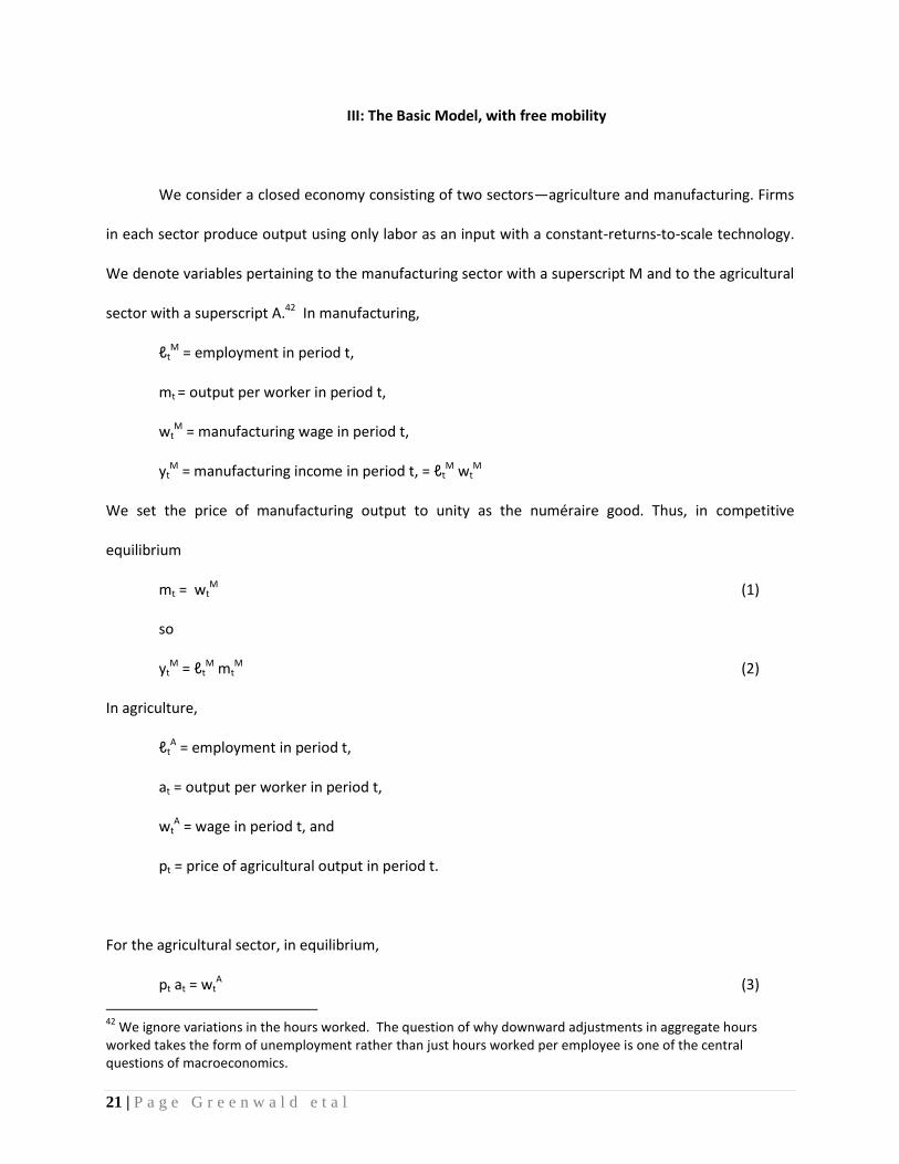
We consider a closed economy consisting of two sectors—agriculture and manufacturing. Firms
in each sector produce output using only labor as an input with a constant-returns-to-scale technology.
We denote variables pertaining to the manufacturing sector with a superscript M and to the agricultural
sector with a superscript A.42 In manufacturing,
ℓtM = employment in period t,
mt = output per worker in period t,
wtM = manufacturing wage in period t,
ytM = manufacturing income in period t, = ℓt
M wtM
We set the price of manufacturing output to unity as the numéraire good. Thus, in competitive
equilibrium
mt = wtM (1)
so
ytM = ℓt
M mtM (2)
In agriculture,
ℓtA = employment in period t,
at = output per worker in period t,
wtA = wage in period t, and
pt = price of agricultural output in period t.
For the agricultural sector, in equilibrium,
pt at = wtA (3)
42
We ignore variations in the hours worked. The question of why downward adjustments in aggregate hours worked takes the form of unemployment rather than just hours worked per employee is one of the central questions of macroeconomics.
22 | P a g e G r e e n w a l d e t a l
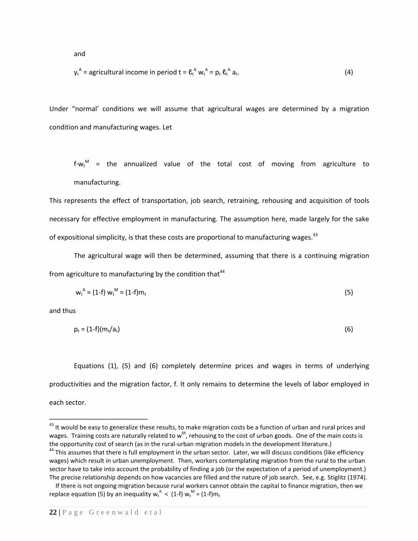
and
ytA = agricultural income in period t = ℓt
A wtA = pt ℓt
A at. (4)
Under “normal’ conditions we will assume that agricultural wages are determined by a migration
condition and manufacturing wages. Let
f·wtM = the annualized value of the total cost of moving from agriculture to
manufacturing.
This represents the effect of transportation, job search, retraining, rehousing and acquisition of tools
necessary for effective employment in manufacturing. The assumption here, made largely for the sake
of expositional simplicity, is that these costs are proportional to manufacturing wages.43
The agricultural wage will then be determined, assuming that there is a continuing migration
from agriculture to manufacturing by the condition that44
wtA = (1-f) wt
M = (1-f)mt (5)
and thus
pt = (1-f)(mt/at) (6)
Equations (1), (5) and (6) completely determine prices and wages in terms of underlying
productivities and the migration factor, f. It only remains to determine the levels of labor employed in
each sector.
43
It would be easy to generalize these results, to make migration costs be a function of urban and rural prices and wages. Training costs are naturally related to w
M, rehousing to the cost of urban goods. One of the main costs is
the opportunity cost of search (as in the rural-urban migration models in the development literature.) 44
This assumes that there is full employment in the urban sector. Later, we will discuss conditions (like efficiency wages) which result in urban unemployment. Then, workers contemplating migration from the rural to the urban sector have to take into account the probability of finding a job (or the expectation of a period of unemployment.) The precise relationship depends on how vacancies are filled and the nature of job search. See, e.g. Stiglitz (1974). If there is not ongoing migration because rural workers cannot obtain the capital to finance migration, then we replace equation (5) by an inequality wt
A < (1-f) wt
M = (1-f)mt
23 | P a g e G r e e n w a l d e t a l
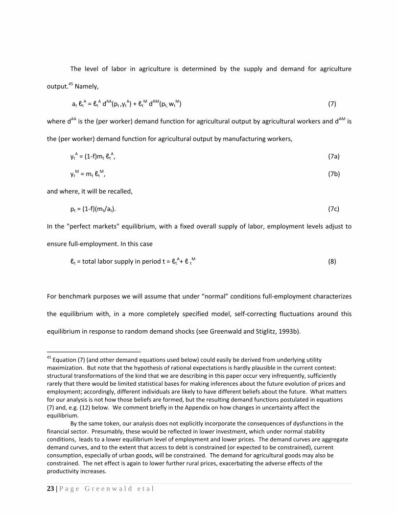
The level of labor in agriculture is determined by the supply and demand for agriculture
output.45 Namely,
at ℓtA = ℓt
A dAA(pt ,ytA) + ℓt
M dAM(pt, wtM) (7)
where dAA is the (per worker) demand function for agricultural output by agricultural workers and dAM is
the (per worker) demand function for agricultural output by manufacturing workers,
ytA = (1-f)mt ℓt
A, (7a)
ytM = mt ℓt
M, (7b)
and where, it will be recalled,
pt = (1-f)(mt/at). (7c)
In the "perfect markets" equilibrium, with a fixed overall supply of labor, employment levels adjust to
ensure full-employment. In this case
ℓt = total labor supply in period t = ℓtA+ ℓ t
M (8)
For benchmark purposes we will assume that under “normal” conditions full-employment characterizes
the equilibrium with, in a more completely specified model, self-correcting fluctuations around this
equilibrium in response to random demand shocks (see Greenwald and Stiglitz, 1993b).
45
Equation (7) (and other demand equations used below) could easily be derived from underlying utility maximization. But note that the hypothesis of rational expectations is hardly plausible in the current context: structural transformations of the kind that we are describing in this paper occur very infrequently, sufficiently rarely that there would be limited statistical bases for making inferences about the future evolution of prices and employment; accordingly, different individuals are likely to have different beliefs about the future. What matters for our analysis is not how those beliefs are formed, but the resulting demand functions postulated in equations (7) and, e.g. (12) below. We comment briefly in the Appendix on how changes in uncertainty affect the equilibrium. By the same token, our analysis does not explicitly incorporate the consequences of dysfunctions in the financial sector. Presumably, these would be reflected in lower investment, which under normal stability conditions, leads to a lower equilibrium level of employment and lower prices. The demand curves are aggregate demand curves, and to the extent that access to debt is constrained (or expected to be constrained), current consumption, especially of urban goods, will be constrained. The demand for agricultural goods may also be constrained. The net effect is again to lower further rural prices, exacerbating the adverse effects of the productivity increases.
24 | P a g e G r e e n w a l d e t a l
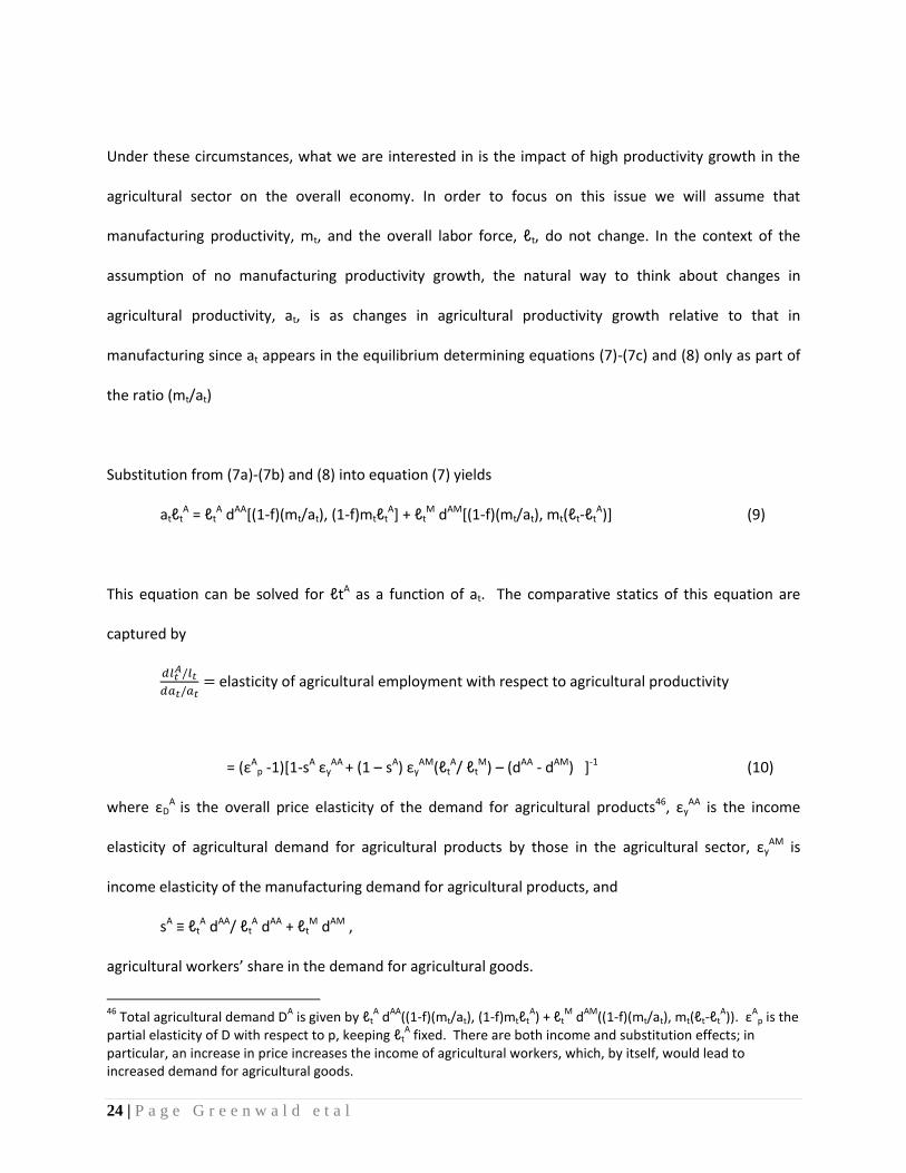
Under these circumstances, what we are interested in is the impact of high productivity growth in the
agricultural sector on the overall economy. In order to focus on this issue we will assume that
manufacturing productivity, mt, and the overall labor force, ℓt, do not change. In the context of the
assumption of no manufacturing productivity growth, the natural way to think about changes in
agricultural productivity, at, is as changes in agricultural productivity growth relative to that in
manufacturing since at appears in the equilibrium determining equations (7)-(7c) and (8) only as part of
the ratio (mt/at)
Substitution from (7a)-(7b) and (8) into equation (7) yields
atℓtA = ℓt
A dAA[(1-f)(mt/at), (1-f)mtℓtA] + ℓt
M dAM[(1-f)(mt/at), mt(ℓt-ℓtA)] (9)
This equation can be solved for ℓtA as a function of at. The comparative statics of this equation are
captured by
elasticity of agricultural employment with respect to agricultural productivity
= (εAp -1)[1-sA εy
AA + (1 – sA) εyAM(ℓt
A/ ℓtM) – (dAA - dAM) ]-1 (10)
where εDA is the overall price elasticity of the demand for agricultural products46, εy
AA is the income
elasticity of agricultural demand for agricultural products by those in the agricultural sector, εyAM is
income elasticity of the manufacturing demand for agricultural products, and
sA ≡ ℓtA dAA/ ℓt
A dAA + ℓtM dAM ,
agricultural workers’ share in the demand for agricultural goods.
46
Total agricultural demand DA is given by ℓt
A d
AA((1-f)(mt/at), (1-f)mtℓt
A) + ℓt
M d
AM((1-f)(mt/at), mt(ℓt-ℓt
A)). ε
Ap is the
partial elasticity of D with respect to p, keeping ℓtA fixed. There are both income and substitution effects; in
particular, an increase in price increases the income of agricultural workers, which, by itself, would lead to increased demand for agricultural goods.
25 | P a g e G r e e n w a l d e t a l
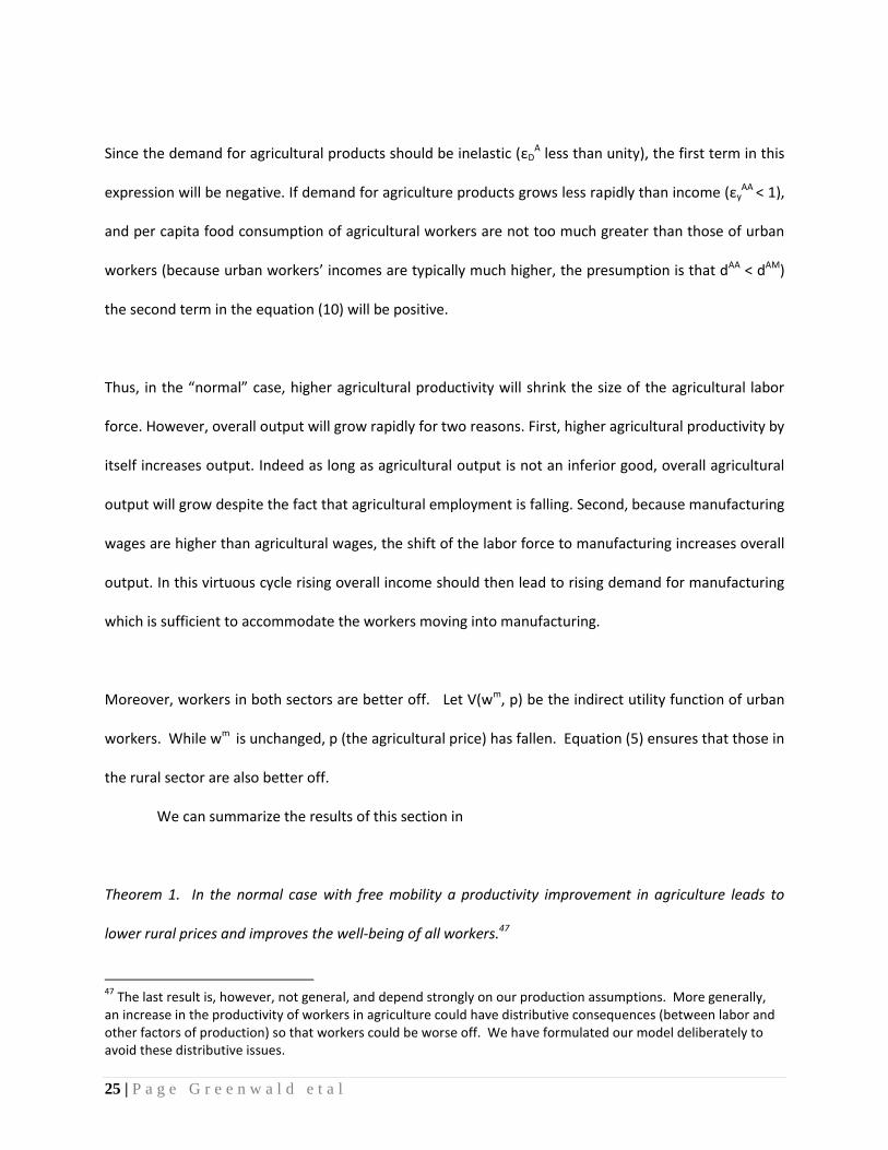
Since the demand for agricultural products should be inelastic (εDA less than unity), the first term in this
expression will be negative. If demand for agriculture products grows less rapidly than income (εyAA < 1),
and per capita food consumption of agricultural workers are not too much greater than those of urban
workers (because urban workers’ incomes are typically much higher, the presumption is that dAA < dAM)
the second term in the equation (10) will be positive.
Thus, in the “normal” case, higher agricultural productivity will shrink the size of the agricultural labor
force. However, overall output will grow rapidly for two reasons. First, higher agricultural productivity by
itself increases output. Indeed as long as agricultural output is not an inferior good, overall agricultural
output will grow despite the fact that agricultural employment is falling. Second, because manufacturing
wages are higher than agricultural wages, the shift of the labor force to manufacturing increases overall
output. In this virtuous cycle rising overall income should then lead to rising demand for manufacturing
which is sufficient to accommodate the workers moving into manufacturing.
Moreover, workers in both sectors are better off. Let V(wm, p) be the indirect utility function of urban
workers. While wm is unchanged, p (the agricultural price) has fallen. Equation (5) ensures that those in
the rural sector are also better off.
We can summarize the results of this section in
Theorem 1. In the normal case with free mobility a productivity improvement in agriculture leads to
lower rural prices and improves the well-being of all workers.47
47
The last result is, however, not general, and depend strongly on our production assumptions. More generally, an increase in the productivity of workers in agriculture could have distributive consequences (between labor and other factors of production) so that workers could be worse off. We have formulated our model deliberately to avoid these distributive issues.
26 | P a g e G r e e n w a l d e t a l
However, constraints on mobility may dramatically alter this picture, and that is what we examine next.
IV: Mobility Constraints
Workers moving from agriculture to manufacturing must usually be able to cover the whole
upfront cost F. Typically only a fraction of agricultural workers will have the necessary savings.48 We will
denote this fraction as γt in period t, where γt will typically vary with fluctuations in agricultural
prosperity. A sequence of poor agricultural years will reduce the value of agricultural investments,
especially local housing, and reduce the number of households able to finance a move to manufacturing.
The amount of surplus labor in agriculture in any given year will depend on the rate of
productivity growth in agriculture. In the previous section we showed that the higher productivity in
agriculture, the lower the demand for agricultural workers. This means that the greater the rate of
productivity growth, the higher the number of workers displaced. If the number of displaced workers
exceeds the number of agricultural workers able to finance the transition to manufacturing, then the
48
For an early discussion of the role of financial constraints in determining migration (and urban-rural equilibrium, in the context of a developing country), see Stiglitz, 1969. Note that in this model, the major effect of a disruption to the financial system is that it would make financing of moving more difficult, i.e. a smaller fraction of the population could obtain the funds required to move. In practice, few individuals actually finance migration through loans. Individuals differ, of course, not only in the access to funds, but in the returns to migration. If all individuals of the same age cohort are identical, then it would be the youngest people who would migrate first (in a world with perfect capital markets), since they could amortize the fixed costs of moving over a longer period. In addition, different individuals face different prospects of getting an urban job. The analogy in terms of transferring from manufacturing (or construction) to a job in services is the limited access to funds for human capital upgrading. Workers need to invest to develop the new skills needed for the new job (as well as move to where job prospects are better).
27 | P a g e G r e e n w a l d e t a l
wage equalization conditions, equation (6), will no longer apply. Formally, if Δat is the change in
agricultural productivity between t – 1 and t, then if
γtℓtA < |d ℓt
A /dat| ·Δat (11)
the agriculture wage will be determined by market clearing conditions in an isolated agricultural labor
market. The resulting equilibrium is self-reinforcing. The limitation on migration increases the
agricultural labor force and reduces agricultural wages from what they would otherwise be. The
reduction in agricultural wages increases agricultural output and reduces agricultural prices and incomes
(under the likely circumstances derived below). The reduction in agricultural incomes reduces the
fraction of agricultural workers able to finance a transition to manufacturing, which further increases
the agricultural labor supply (from what it would have been in the unconstrained migration
equilibrium.)49 In the end migration may essentially evaporate and, in equilibrium, further increases in
agricultural productivity will lead to further immiseration of the now trapped population of agricultural
workers.
Lower agricultural incomes, in turn, undermines demand for manufactured goods and may lead
to overall economic stagnation. Thus, if productivity growth in agriculture is high enough and/or
agricultural workers' ability to finance migration is impaired enough (γt falls enough), a transition to a
long-lived inferior equilibrium may replace the virtuous cycle of the previous section.
49
There is an alternative formulation that gives more ambiguous results, with the possibility of intermittent periods of migration. Assume that that there is a distribution of costs of capital. Then migration occurs to the
point where the annualized cost of migration equals – (assuming static expectations.) If, for the individual
with the lowest cost of capital, the cost of migration exceeds – then there will be no migration. But a fall in the agricultural wage relative to the urban wage might induce migration, even if worsening conditions in the agricultural sector led to an increase in cost of capital even for the individual with the lowest cost of capital. (In the efficiency wage version, to be discussed below, there is urban unemployment; what matters for migration is expected lifetime income of an individual who migrates to the city. That depends on how the urban labor market functions, e.g. if there is a daily labor market, so the expected wage is (1 – U) wm, or whether there is a queue for jobs, with migrants coming at the end of the queue. See Stiglitz (1974).

28 | P a g e G r e e n w a l d e t a l
To model this equilibrium, we will no longer assume that agricultural wages are determined by
the migration condition of equation (6). Instead we will assume that ℓtA is fixed and wages in agriculture
are set at a level necessary to employ this labor force. We will continue to assume that there are
constant-returns-to-scale in production in agriculture and that labor is the only input.
In the “normal” equilibrium, as surplus labor migrated from agriculture to manufacturing, the
rise in average wages generated sufficient income to absorb the greater level of manufacturing output.
In the no-mobility equilibrium, there is no longer any need to absorb surplus agricultural labor into the
manufacturing sector. But, the steady decline in agriculture incomes may, under circumstances outlined
below, actually reduce the overall demand for manufacturing in the short run and, as the decline in
agricultural incomes continues, in a longer run as well. The low income in agriculture not only weakens
demand in the urban sector, but the weaker urban economy has repercussions back to the agricultural
sector.
In this section, we assume that wages in the urban sector adjust to maintain full employment.
In the next, we assume that wage rigidities lead to unemployment in the urban sector.
We generalize the model slightly to assume that different workers in the urban sector have
different reservation wages, so that while potential labor supply in the urban sector is ℓtM, actual
employment is E(wt m) ≤ ℓt
M, and that output in the urban sector is H(E). We focus on the situation
where E = E(wt m), i.e. there is full employment in the urban sector, in the sense that everyone who
wants a job at the going wage (wtM-) can get one. Inverting, we obtain
wtM = E-1(Et ) ≡ ξ (Et )
Equilibrium agricultural prices are now determined by50
at ℓtA = ℓt
A dAA(pt , pt at ) + Et dAM(pt, ξ (Et )) (12a)
50
This equation might be interpreted as suggesting that those in the urban sector who are not employed have zero demand for food. A better way of thinking of equation (12a) is urban demand depends on urban income (E ξ (Et )) and relative prices, p: D
AM= D
AM (E ξ (Et )),p), where D
AM is total urban demand for agricultural goods. We have
simplified by assuming that DAM
takes on the special form: Et dAM
(pt, ξ (Et )). But the analysis does not depend on this parameterization.
29 | P a g e G r e e n w a l d e t a l
where ℓtA is now fixed by a no migration constraint. Equilibrium requires demand to equal supply:
H(E t) = ℓtA dAM (pt , pt at) + Et d
MM (pt ξ (Et ) ) +It (12b)
where dAM (dMM) is demand from those in the agricultural (manufacturing) sector for manufacturing
goods, and I is the level of investment (assumed to be industrial goods).
(12a) - (12b) can be solved simultaneously for {Et, pt } for any given value of at. The curve AA
gives the equilibrium combinations of urban employment (wages) and rural prices which clear the
agricultural market: for any given at, the higher urban employment (wages), the higher rural prices.
The curve MM in Figure 1 gives the equilibrium combinations of urban employment (wages)
and rural prices which clear the urban (manufacturing) market. Higher urban employment (wages)
increases supply (assuming that all workers who want to work are employed) and demand, but stability
implies that the effect on supply exceeds the effect on demand (otherwise, as labor is hired to meet a
shortfall of production and wages get bid up, demand would increase more than supply, and the
shortfall would increase).51 At the same time, higher rural prices increase demand, both because
farmers’ income is higher, and because consumers substitute urban goods for rural goods. Hence, as p
increases, equilibrium urban employment and wages increase.
[Figure 1 about here]
Since both curves are upward sloping, there can be more than one equilibrium as illustrated in
the figure—a high urban employment (wage)/higher rural price equilibrium, and a low urban
employment (wage)/low rural price equilibrium. Clearly, from the perspective of rural workers the
51
Technically, we assume that H’(E) > Et dMM
y ξ ‘(Et ) + dMM
, or h > sMM
(εdMMy μ + 1), where h = dln H/dln E, the elasticity of output with respect to employment, s
MM is the share of total manufactured goods purchased by urban
workers, εdMMy is the income elasticity of demand for urban goods by urban workers, and μ ≡ d ln ξ (Et )/ dln E, the percentage change in wages from a one percent increase in employment along the labor supply curve (the inverse of the labor supply elasticity.)
30 | P a g e G r e e n w a l d e t a l
former is preferable to the latter, and, under plausible conditions, so is it preferable for the urban
workers.52 For the rest of this paper, we focus on the case where there is a unique, stable equilibrium.
It can be shown that a “natural” stability condition requires the AA curve to be flatter than the MM
curve. Thus, we focus our analysis on the high price and employment equilibrium in Figure 1, and how it
shifts as agricultural productivity increases.
The effect of rising agricultural productivity is to sharply decrease agricultural incomes. The AA
curve shifts down (at any level of urban employment and income, the market clearing level of
agricultural prices is lower). At the same time, the MM curve shifts to the right: at any given rural price,
rural incomes are higher, and so will the demand for urban goods. Under plausible conditions, however,
the new equilibrium entails both lower urban employment (wages) and rural prices, and both urban and
rural workers are worse off. With restricted mobility, the productivity improvement in the rural sector
leads to universal immiseration.53 (See Figure 2)
[Figure 2 about here]
We summarize the results of this section in
Theorem 2. Normally, with restricted mobility, an increase in agricultural productivity leads to both
lower urban wages and lower rural prices, and both rural and urban workers are worse off.
52
From the indirect utility function, we require (1 + μ) > σ MA
(dln p/dln E)AA where σ MA
is the average propensity of those in the urban sector to consume agriculture goods (≡ pd
MA/w) and (dln p/dln E)AA denotes the elasticity of
the AA curve. If σ
MA is small enough, and the AA curve is flat enough (increases in urban employment have a
relatively small effect on the market clearing price in the rural sector) it is clear that urban workers are better off at the high price equilibrium. The slope of the AA curve can, in turn, be related to demand elasticities and labor supply elasticities. 53
The condition is simply that, at a fixed urban wage (employment level), the decrease in price as at increases in the agricultural sector (i.e. for the AA curve) is greater than the decrease in in the urban sector (i.e. for the MM curve). For the former, dln p/d ln a = - (1 – s
A ey
AA ) /ε
Ap and for the latter, dln p/d ln a = – s
M ey
AM / ε
M1/p, where ey
Ai is the income
elasticity of sector i goods of agricultural workers, sM
is the share of urban goods consumed by rural workers, εA
p is the (absolute value of) price elasticity of agricultural goods, and ε
M1/p is the (absolute value of) price elasticity of
manufactured goods (noting that the relative price of urban goods is 1/p). Normally, we would expect 1 – sA ≥ s
M
with strict inequality if there is savings; and low income elasticities (especially for food) so that (1 – sA ey
AA) > s
M
eyAM
, i.e. 1 > sA ey
AA +s
M ey
AM and ε
Ap << ε
M1/p—food consumption is also price inelastic. We will refer to the case
where (1 – s
A ey
AA ) /ε
Ap > s
M ey
AM / ε
M1/p and where the stability condition is satisfied as the “normal case.”
31 | P a g e G r e e n w a l d e t a l
V: Efficiency Wages and Induced Unemployment
In the previous section, we assumed only one market imperfection—there was a constraint on
labor mobility. Markets still cleared in both the urban and rural sectors. If, however, wages are not fully
flexible, e.g. because of efficiency wages, then there will be involuntary unemployment (as opposed to
the voluntary decision not to supply labor, discussed in the previous section.)
For simplicity, consider first the case where wages are totally rigid54, but there is zero labor
supply elasticity. We then replace equations (12) with equations (13)
at ℓtA = ℓt
A dAA(pt , ytA) + Et d
AM(pt ,w*) (13a)
H’(Et)= ℓtAdAM (pt , pt at) + Et d
MM (pt ,w* ) +It (13b)
(13a) and (13b ) can be solved simultaneously for {pt, Et}. The analysis parallels that of the previous
section, but now, the welfare costs of the productivity increase in agriculture are greater, because it
gives rise to induced urban unemployment.
It is possible to show (as before)
Theorem 3. “Normally,” with stability, equilibrium employment and prices will decrease as agriculture
productivity increases.
The equilibrium can be illustrated in a figure identical to Figure 2. Stability again requires that the slope
of the MM curve, giving the pair of {p,E} for which the demand for manufactured goods equals the
supply (eq. 13b is satisfied) be greater than the slope of the AA curve (the set of {p,E} for which the
54
It is easy to generalize these results to the case where the efficiency wage is, itself, a function of the employment (unemployment) level, as in the standard Shapiro-Stiglitz no-shirking model. We then replace w* with a function, w*(E).
32 | P a g e G r e e n w a l d e t a l
agricultural market clears). The footnote provides sufficient conditions for this condition to be satisfied
in terms of the underlying demand and supply functions.55
A special parameterization. The results can be seen especially easily in the following special
parameterization. Assume
Et mt = I+EcM(w*-pt dAM)+ ℓt
AcA(ytA-ptd
AA)
where individuals first decide on how much food to eat (food is a necessity, which is totally price
inelastic) and then workers in the urban sector spend a fraction of the residual, cM on urban goods, and
similarly for agricultural workers. Assume, further, that rural workers are limited in the amount that
they can spend on manufactured goods to what they receive from urban workers, and that they do in
fact spend that amount (a kind of balance of trade condition).56 Hence
EpdAM = ℓtA cA [pa – pdAA]
Substituting, we obtain
Et mt = I+Et cM(w*t
M-pt dAM)+ EpdAM
or
55
Define, as before, DA (p; E) ≡ ℓ
Ad
AA (p, pα) + Ed
MA (p , w* ) as total demand in the agricultural sector, and define
DM
(p, E) similarly. Then the slope (elasticity) of the AA curve is given by - EdMA
/pDA
p = (1 – sAA
)/εA
p where εA
p is the price elasticity of total demand in the agricultural sector (now, keeping E and ℓ
A fixed) and s
AA is the share of
consumption of food by those in the agricultural sector. The elasticity of the MM curve is –(H’E – Ed
MM )/pd
Mp = h – s
MM/ε
Mp, where, it will be recalled, s
MM is the share of
manufactured goods consumed by those in the urban sector, and εM
p is the (absolute value of the) elasticity of demand of manufactured goods with respect to the agricultural price. When the price of agricultural goods increases, there are two effects: a substitution effect away from food and towards manufactured goods, and an increase in real incomes of those in the rural sector and a decrease of those in the urban sector. In a representative agent model, the redistribution effects cancel and there is only the substitution effect. If the elasticity of substitution is low, ε
Mp will be small. On the other hand, an increase in agricultural prices results in a
substitution effect against agriculture (again related to the elasticity of substitution) combined with an income effect (farmers are better off, urban workers worse off). Hence, we assume (h – s
MM )/ε
Mp > ( 1 – s
AA )/ε
Ap . If price elasticities (appropriately defined) are approximately the
same, then stability (AA being flatter than MM) simply requires that (h – sMM
) > ( 1 – sAA
). This will be true if sAA
> s
MM and h is near unity , i.e. agriculture workers consume a larger fraction of their own goods than urban workers’
share of consumption (production) of their own good. 56
If it were not satisfied, it would mean that rural workers were getting increasingly indebted to the urban sector—they would be buying more than they are selling—or that they were saving (paying back prior debts). Given the constraints in financial markets, the former does not seem plausible; and in the presence of large declines in incomes, neither does the latter. This assumption allows us to greatly simplify the analysis.
33 | P a g e G r e e n w a l d e t a l
E = I / mt – [cM(w*tM-pt d
AM)+ pdAM],
so
dE/dp = EdAM(1 – cM)/ mt - cM(w*-pt d
AM) -pdAM
= EdAM(1 – cM)/ {(mt – w*)+ (1- cM )(w*-pt dAM)}
Assume, for instance, that those in the urban sector consume all of their “excess” income, so cM = 1.
Then,
dE/dp = 0.
The MM line is perfectly vertical at
E = I /mt – w*tm
Section VI: Policy
Government interventions can improve matters. In this section, we explore three possible
interventions: fiscal policy, wage policies, and policies to facilitate migration.
5.1 Impact of Keynesian stimulus
Assume now that we introduce government spending, replacing equation (13b) with
(14) H(Et)= ℓtADAM (pt , pt at) + Et D
MM (pt ,w* ) + It + G.
It immediately follows that even though the origins of the crisis was structural, a Keynesian (fiscal)
stimulus (an increase in G) increases both employment and rural prices. As G increases, MM shifts to the
right, as in Figure 3.
Theorem 4: Under the stability condition57, an increase in government expenditure increases urban
employment and raises agricultural prices and incomes.58
57
Defined earlier as the AA curve being flatter than the MM curve. 58
By hypothesis, we assume that Ricardian equivalence does not hold, so that the future tax liabilities do not lead to an equal and offsetting reduction in consumption today. This follows naturally from our assumptions of capital market imperfections, which underlies the entire analysis.
34 | P a g e G r e e n w a l d e t a l
[Figure 3 about here]
5.2 The effects of wage adjustments
We have assumed that urban wages are fixed, e.g. as a result of efficiency wages. Different efficiency
wage theories provide different predictions for what might happen to real wages denominated in
manufactured goods when food prices fall.59 Some versions (such as labor turnover theories) are
consistent with no changes in real wages, denominated in manufactured goods. Others, such as the
Shapiro-Stiglitz incentives-based model, predict a decline in real wages, denominated in manufactured
goods.
By the same token, many economists have blamed unemployment on excessively high wages. But in our
model—as almost surely in the real world in a severe economic downturn such as the Great Recession
or Great Depression—the effect on demand of falling wages worsens the downturn. A decrease in
urban real wages shifts down the AA curve (demand for food decreases with the decrease in urban
workers' incomes), which lowers employment and prices further. Such decreases did, of course, occur
in the Great Depression. But now, the second round effect in the urban sector reinforces this effect. At
any level of employment, for demand for urban goods to equal supply, the price of urban goods has to
fall, i.e. the price of rural goods has to rise, implying that the MM curve shifts up, so that in equilibrium,
urban employment is lowered even more (and agricultural goods prices are further lowered.)60
59
For a discussion, see, e.g. Sah and Stiglitz (1992) 60
Keynes anticipated this effect: "if labour were to respond to conditions of gradually diminishing employment by offering its services at a gradually diminishing money-wage, this would not, as a rule, have the effect of reducing real wages and might even have the effect of increasing them, through its adverse influence on the volume of output. The chief result of this policy would be to cause a great instability of prices, so violent perhaps as to make business calculations futile in an economic society functioning after the manner of that in which we live” (Keynes 1936, Chapter 19). The quotation makes clear that Keynes did not think that the "solution" to unemployment was to lower wages. Our model is consistent with this result, in that output falls, and since agricultural prices fall, real wages in agricultural goods could actually rise, and is likely to do so if the MM curve is very steep.
35 | P a g e G r e e n w a l d e t a l
[Figure 4 about here]
Theorem 5: Under the stability condition., a decrease in urban real product wages increases urban
unemployment and lowers agricultural prices and incomes.
5.3. Migration subsidies
Assume the government could facilitate migration, i.e. reduce ℓtA
. What happens to the equilibrium? We
focus our discussion here on the unemployment equilibrium of section IV. From equation (13), it is clear
that the AA curve shifts upwards (at each E , the equilibrium agricultural price increases, since net
supply—output minus consumption by agricultural workers—decreases). By itself, this leads to more
urban employment. The MM curve, on the other hand, shifts to the left—at each p, demand for urban
goods decreases, so employment falls. The net effect would appear to be ambiguous, but under
“normal” conditions, employment increases—given the price inelasticity, the decreased supply has a
larger impact on agricultural prices and income (and therefore urban employment) than the fact that, at
any price, there are fewer rural workers demanding urban goods.
[Figure 5 about here]
Section VII: Global Interactions
In a closed economy agricultural demand is limited to local demand. In a global economy individual local
economies can sustain employment in their agricultural sector by exporting into a global market. In
particular by devaluing its currency, any small country can increase output (although not the
international price at which it sells that output.) The advantages of doing so are threefold. First, the
local terms of trade between manufactures (urban goods) and agricultural products (the rural sector)
36 | P a g e G r e e n w a l d e t a l
can be improved. To the extent that there are manufactured goods locally produced and consumed
(including, and especially non-traded manufactured goods), a devaluation of the local currency which
raises the local price of agricultural output will increase the local currency value of rural income and
have a positive effect on rural demand for manufacturers. Second, if agricultural debts are denominated
in local currency, the devaluation will reduce the level of these debts relative to agricultural income and
perhaps relax the agricultural mobility constraint. Third, the rise in local currency agricultural incomes
may by itself relax the mobility constraint, specifically if migration costs are set in local currency terms.
These factors apply (mutatis mutandi) with special force today in the transition from
manufactures which are traded globally and are experiencing high current rates of productivity growth
to services which are overwhelmingly locally produced and consumed.
The problem with attempting to capture a greater share of international demand is that not all
countries can succeed in doing so. Surpluses and deficits across all countries must sum to zero. What
matters is relative prices—exchange rates—and a country’s trading partners can largely undo whatever
a country does to lower its exchange rate. It is only if some countries cannot devalue their currencies
either because they are reserve currencies against which all other currencies are measured (e.g. US) or
because they are part of a common currency area (e.g. Greece, Spain, Portugal, Italy and the other Euro
countries), that they can be taken advantage of in a global context.
In this connection, it is significant that relatively small countries like Australia and Argentina
which devalued their currencies early in the Depression were able successfully to limit the short run
impact of increasing global agricultural productivity. The adverse impact on reserve currency countries
or those that adhered strictly to the gold standard like the UK and the US was much more severe.
In the present crisis reserve currency countries like the US with very limited manufacturing
employment (relative to total employment) have still suffered from prolonged deflationary pressure.

37 | P a g e G r e e n w a l d e t a l
Other countries, such as Germany, Korea, and China, which have large manufacturing sectors but have
been able to limit the appreciation of their currencies, have fared unexpectedly well.

38 | P a g e G r e e n w a l d e t a l
VIII: Conclusion
We argue here that the relatively rare long-lived deflationary episodes arise from significant real
structural economic dislocations. Data presented here show that the Depression in the United States
was related to the decline of agriculture arising from the large increase in agricultural productivity. As
farm income—the income of almost 30% of the population at that time—fell in the 1920’s, workers left
the sector. But then in current dollars it fell by more than half from 1929 to 1932. Despite the relative
decline in farm returns, the agricultural population, which fell from 30 percent to 24.8 percent of the US
population over the course of the 1920s, actually rose slightly in 1930s (although it did fall as a percent
of the total population). Workers were “trapped” in the rural sector, reinforcing the income declines,
the effects of which were then felt strongly in the urban sector. The limited increases in government
spending could not offset the impact of declining agricultural incomes. With trapped labor, productivity
growth, rather than raising standards of living for all, could lower welfare.
World War II and the policies that were pursued in its aftermath had a major structural impact
on the US economy. These policies succeeded in helping the economy make the transformation that it
was unable to do on its own. In the 1940s with the impetus of war-driven dislocations, the agricultural
population fell sharply to 15.2 percent, with the vast majority of the shift occurring between 1940 and
1945.61 Today the challenge is to shift workers out of manufacturing into services. This will have to be
done globally. But globalization has made the global economy especially sensitive to shifting
comparative advantages. In the shift from agriculture to manufacturing, the US continued to be a strong
producer of agricultural goods, even as employment diminished, simply because there was an
abundance of one of the critical factors, productive land. That may happen in some manufacturing
sectors, where US production continues apace, but with a fraction of the employment. But the
dislocations may be larger, since in some sectors, there may be little reason that production should 61
It continued to fall rapidly in the 1950s and 1960s.
39 | P a g e G r e e n w a l d e t a l
continue at all inside the US. Employment will then decrease both because of the increase in
productivity and because of the loss of comparative advantage. Some countries may attempt to invest,
to restore their dynamic comparative advantage; but from a global perspective, this cannot be a
“solution” to the problem of declining global manufacturing employment. Indeed, to some extent, it will
exacerbate the problems, because the struggle to achieve dynamic comparative advantage will normally
be through further increases in productivity—meaning even less manufacturing employment.
If global growth continues to remain as robust as it has been at its peak, at some 4%62, global
growth in the demand for manufactured goods may fall only slightly short of the amazing growth in
manufacturing productivity (or may even slightly exceed it). In that case, the fight will be over where
the relatively fixed set of manufacturing jobs are located. For the world as a whole, the share of
employment in manufacturing will almost surely decline significantly, and in the longer run, almost
surely, productivity growth will outpace demand growth. Thus, in the long run, the countries that will
face the most serious adjustment problems are those that, in the short run, remain committed to strong
manufacturing sectors supported by exports and ultimately low exchange rates. For most countries,
continuing commitments to jobs in manufacturing (just as many countries remained committed to
agricultural employment throughout the 1930s) in the face of adverse productivity and demand
conditions is a recipe for problems, if not now, later .
Poorly managed transitions lead to financial sector problems—or crises—which, in turn, impede
the transition. The underlying weaknesses that our analysis has uncovered can, temporarily, be covered
up by a credit bubble, the breaking of which can (as in the current crisis) make the transition all the
more difficult, compounding the challenges of transition with excess capacity in, say, real estate.
62
Estimates of growth based on exchange rates are lower than those based on purchasing power parity. The latter is probably more relevant for estimating the growth in the demand for manufactures.
40 | P a g e G r e e n w a l d e t a l
As in the case of the transition out of agriculture, this transition will require major, carefully
conceived government intervention. Section 5 showed that even though the underlying problem may
be considered structural, austerity, of the kind currently being contemplated in Europe and America,
leads to higher unemployment. Keynesian policies can help address the unemployment problem, even
when the origins are linked with structural transformation. Well-targeted industrial policies can have an
even more positive effect. There is one more aspect of the current transition which suggests that
austerity is likely to have an even more adverse effect than our analysis suggested. This is a transition
from manufacturing to services, and among the services most in demand, and likely to provide
employment for those transitioning out of manufacturing, are health and education, sectors in which
government finance has, for good reasons, traditionally been important. Austerity will especially
weaken demand in these sectors, making the plight of those trapped in the declining sectors all the
worse.
This paper has not only argued that underlying current economic difficulties is a “real” shock to
the economy, but also explained why the single-minded focus on the financial sector is misguided. The
aftermath of a real estate bubble, the overhang of debt and low real estate prices, caused by financial
sector mismanagement does make the transition all the more difficult. Moreover, failing to fix the
financial and real estate sectors almost surely will impede the transition. In the end, though, “fixing” the
financial sector does not, itself, “solve” the transition problem. That requires, first, recognizing that this
is the underlying problem facing the economy today, and second, designing a package of fiscal,
structural, and financial responses that will facilitate a more rapid transition.
41 | P a g e G r e e n w a l d e t a l
References
Adrian, T., Shin, H. (2008) ‘Liquidity and Leverage’, Federal Reserve Bank of New York Staff Report #398.
Atkinson, A.B., Piketty, T., and E. Saez (2011) ‘Top Incomes in the Long Run of History’, Journal of Economic Literature, vol. 49(1)1, 3–71.
Bates, T.W., K.M. Kahle and R.M. Stulz (2009) ‘Why Do U.S. Firms Hold So Much More Cash than They Used To?’ Journal of Finance, vol. 64(5), pp. 1985-2021.
Bell, S. (1940) Productivity, Wages and National Income (Washington, D.C.: The Brookings Institution).
Bernanke, B., M. Gertler and S. Gilchrist (1999) ‘The Financial Accelerator in Quantitative Business Cycle Framework’, in Handbook of Macroeconomics, Vol. 1C, edited by L. Taylor and M. Woodford (Amsterdam: North Holland).
Carter, S.B., S.S. Gartner, M.R. Haines, A.L. Olmstead, R. Sutch and G. Wright, eds. (2006) Historical Statistics of the United States, Millennial Edition Online, (Cambridge: Cambridge University Press).
Chandler, L.V. (1970) America’s Greatest Depression (New York: Harper and Row).
Dynan, K.E., J. Skinner and S.P. Zeldes (2004), ‘Do the Rich Save More?’ Journal of Political Economy, University of Chicago Press, vol. 112(2), pp. 397-444.
Easterly, W., R. Islam and J. E. Stiglitz (2001a) ‘Shaken and Stirred: Explaining Growth Volatility’, Annual Bank Conference on Development Economics 2000 (Washington: World Bank), pp. 191-212.
Easterly, W., R. Islam and J. E. Stiglitz (2001b) ‘Volatility and Macroeconomic Paradigms for Rich and Poor Countries’, in Advances in Macroeconomic Theory: Volume 1, IEA Conference vol. 133, edited by Jacques H. Drèze (Houndsmill: Palgrave), pp. 353-372.
Eggertsson, G.B., and P. Krugman (2010) ‘Debt, Deleveraging, and the Liquidity Trap: A Fisher-Minsky-Koo Approach’, mimeo, Princeton University.
Field, A. (2011) A Great Leap Forward: 1930s Depression and Economic Growth (New Haven: Yale University Press).
Friedman, M., and A.J. Schwartz (1963) A Monetary History of the United States, 1867–1960 (Princeton, NJ: Princeton University Press).
Greenwald, B., and M. Kahn (2008) Globalization: The Irrational Fear that Someone in China will Take Your Job (New York: Wiley).
Greenwald, B., and J.E. Stiglitz, (1988) ‘Examining Alternative Macroeconomic Theories’, Brookings Papers on Economic Activity, vol. 1, pp. 207-270
Greenwald, B., and J.E. Stiglitz (1993a) ‘New and Old Keynesians’, Journal of Economic Perspectives, vol. 7(1), Winter 1993, pp. 23-44.
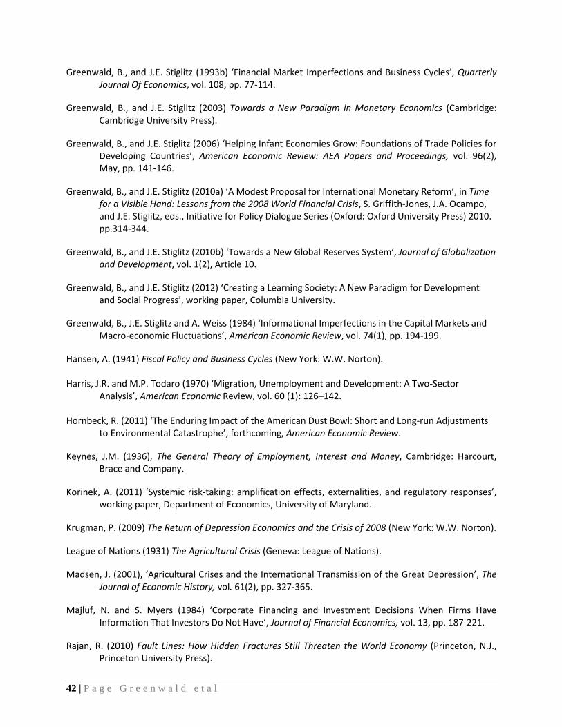
42 | P a g e G r e e n w a l d e t a l
Greenwald, B., and J.E. Stiglitz (1993b) ‘Financial Market Imperfections and Business Cycles’, Quarterly Journal Of Economics, vol. 108, pp. 77-114.
Greenwald, B., and J.E. Stiglitz (2003) Towards a New Paradigm in Monetary Economics (Cambridge: Cambridge University Press).
Greenwald, B., and J.E. Stiglitz (2006) ‘Helping Infant Economies Grow: Foundations of Trade Policies for Developing Countries’, American Economic Review: AEA Papers and Proceedings, vol. 96(2), May, pp. 141-146.
Greenwald, B., and J.E. Stiglitz (2010a) ‘A Modest Proposal for International Monetary Reform’, in Time for a Visible Hand: Lessons from the 2008 World Financial Crisis, S. Griffith-Jones, J.A. Ocampo, and J.E. Stiglitz, eds., Initiative for Policy Dialogue Series (Oxford: Oxford University Press) 2010. pp.314-344.
Greenwald, B., and J.E. Stiglitz (2010b) ‘Towards a New Global Reserves System’, Journal of Globalization and Development, vol. 1(2), Article 10.
Greenwald, B., and J.E. Stiglitz (2012) ‘Creating a Learning Society: A New Paradigm for Development and Social Progress’, working paper, Columbia University.
Greenwald, B., J.E. Stiglitz and A. Weiss (1984) ‘Informational Imperfections in the Capital Markets and Macro-economic Fluctuations’, American Economic Review, vol. 74(1), pp. 194-199.
Hansen, A. (1941) Fiscal Policy and Business Cycles (New York: W.W. Norton). Harris, J.R. and M.P. Todaro (1970) ‘Migration, Unemployment and Development: A Two-Sector
Analysis’, American Economic Review, vol. 60 (1): 126–142. Hornbeck, R. (2011) ‘The Enduring Impact of the American Dust Bowl: Short and Long-run Adjustments
to Environmental Catastrophe’, forthcoming, American Economic Review.
Keynes, J.M. (1936), The General Theory of Employment, Interest and Money, Cambridge: Harcourt, Brace and Company.
Korinek, A. (2011) ‘Systemic risk-taking: amplification effects, externalities, and regulatory responses’, working paper, Department of Economics, University of Maryland.
Krugman, P. (2009) The Return of Depression Economics and the Crisis of 2008 (New York: W.W. Norton).
League of Nations (1931) The Agricultural Crisis (Geneva: League of Nations).
Madsen, J. (2001), ‘Agricultural Crises and the International Transmission of the Great Depression’, The Journal of Economic History, vol. 61(2), pp. 327-365.
Majluf, N. and S. Myers (1984) ‘Corporate Financing and Investment Decisions When Firms Have Information That Investors Do Not Have’, Journal of Financial Economics, vol. 13, pp. 187-221.
Rajan, R. (2010) Fault Lines: How Hidden Fractures Still Threaten the World Economy (Princeton, N.J., Princeton University Press).
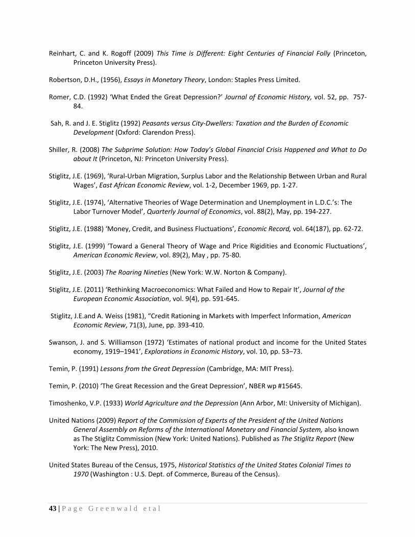
43 | P a g e G r e e n w a l d e t a l
Reinhart, C. and K. Rogoff (2009) This Time is Different: Eight Centuries of Financial Folly (Princeton, Princeton University Press).
Robertson, D.H., (1956), Essays in Monetary Theory, London: Staples Press Limited.
Romer, C.D. (1992) ‘What Ended the Great Depression?’ Journal of Economic History, vol. 52, pp. 757-84.
Sah, R. and J. E. Stiglitz (1992) Peasants versus City-Dwellers: Taxation and the Burden of Economic Development (Oxford: Clarendon Press).
Shiller, R. (2008) The Subprime Solution: How Today’s Global Financial Crisis Happened and What to Do about It (Princeton, NJ: Princeton University Press).
Stiglitz, J.E. (1969), ‘Rural-Urban Migration, Surplus Labor and the Relationship Between Urban and Rural Wages’, East African Economic Review, vol. 1-2, December 1969, pp. 1-27.
Stiglitz, J.E. (1974), ‘Alternative Theories of Wage Determination and Unemployment in L.D.C.’s: The Labor Turnover Model’, Quarterly Journal of Economics, vol. 88(2), May, pp. 194-227.
Stiglitz, J.E. (1988) ‘Money, Credit, and Business Fluctuations’, Economic Record, vol. 64(187), pp. 62-72.
Stiglitz, J.E. (1999) ‘Toward a General Theory of Wage and Price Rigidities and Economic Fluctuations’, American Economic Review, vol. 89(2), May , pp. 75-80.
Stiglitz, J.E. (2003) The Roaring Nineties (New York: W.W. Norton & Company).
Stiglitz, J.E. (2011) ‘Rethinking Macroeconomics: What Failed and How to Repair It’, Journal of the European Economic Association, vol. 9(4), pp. 591-645.
Stiglitz, J.E.and A. Weiss (1981), “Credit Rationing in Markets with Imperfect Information, American Economic Review, 71(3), June, pp. 393-410.
Swanson, J. and S. Williamson (1972) ‘Estimates of national product and income for the United States economy, 1919–1941’, Explorations in Economic History, vol. 10, pp. 53–73.
Temin, P. (1991) Lessons from the Great Depression (Cambridge, MA: MIT Press).
Temin, P. (2010) ‘The Great Recession and the Great Depression’, NBER wp #15645.
Timoshenko, V.P. (1933) World Agriculture and the Depression (Ann Arbor, MI: University of Michigan).
United Nations (2009) Report of the Commission of Experts of the President of the United Nations General Assembly on Reforms of the International Monetary and Financial System, also known as The Stiglitz Commission (New York: United Nations). Published as The Stiglitz Report (New York: The New Press), 2010.
United States Bureau of the Census, 1975, Historical Statistics of the United States Colonial Times to 1970 (Washington : U.S. Dept. of Commerce, Bureau of the Census).

44 | P a g e G r e e n w a l d e t a l
Zandi, M., 2011, ‘To Shore Up the Recovery, Help Housing’, Special Report, Moody’s Analytics, 25 May 2011.
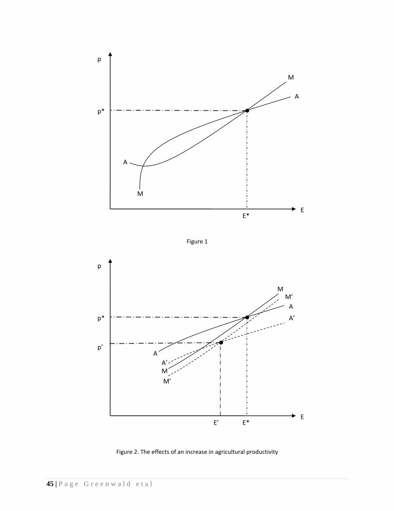
45 | P a g e G r e e n w a l d e t a l
Figure 1
Figure 2. The effects of an increase in agricultural productivity
E
p
A
M
M
A
E*
p*
E
p
A
M
M
A
A’
A’
M’
M’
E*
p*
E’
p’

46 | P a g e G r e e n w a l d e t a l
Figure 3. Impact of Keynesian stimulus:
an increase of G shifts the MM curve shifts from M’M’ to M’’M’’ and increases both employment and rural prices.
E
p
A
M
M
A
A’
A’
M’
M’
E*
p*
E’
p’
M’’
M’’
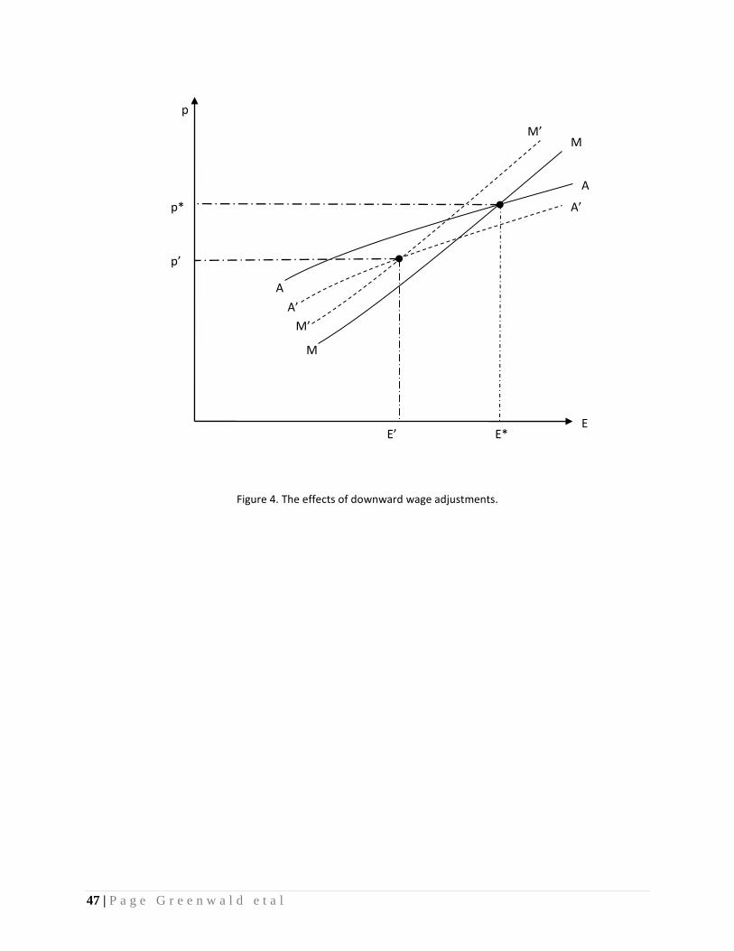
47 | P a g e G r e e n w a l d e t a l
Figure 4. The effects of downward wage adjustments.
E
p
A
M
M
A
A’
A’
M’
M’
E*
p*
E’
p’
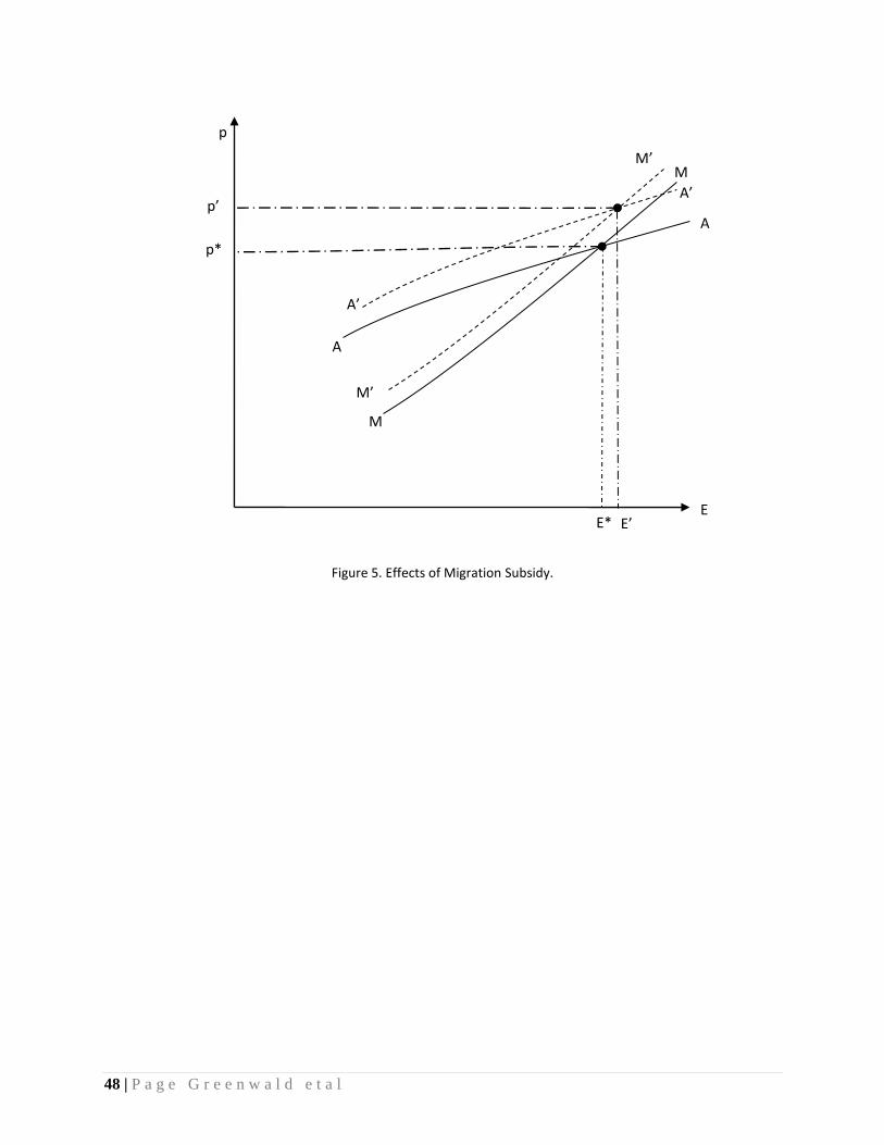
48 | P a g e G r e e n w a l d e t a l
Figure 5. Effects of Migration Subsidy.
E
p
A
M
M
A
A’
A’
M’
M’
E*
p*
E’
p’