SECTION ONE Equipment Design

S E C T I O N O N E

Equipment Design

H7856-Ch001.qxd 7/4/05 6:44 PM

1Fluid Flow

Velocity Head............................................................... 3Full Plant Piping ......................................................... 4Partially Full Horizontal Pipes.................................. 5Equivalent Length....................................................... 6Recommended Velocities ............................................ 7Two-phase Flow........................................................... 9Compressible Flow—Short (Plant) Lines.................12Compressible Flow—Long Pipelines ........................18Sonic Velocity...............................................................21Metering.......................................................................21Control Valves .............................................................22Safety Relief Valves.....................................................25

2

H7856-Ch001.qxd 7/4/05 6:44 PM

Fluid Flow 3

Sonic Velocity

For the situations covered here, compressible fluidsmight reach sonic velocity. When this happens, furtherdecreases in downstream pressure do not produce addi-tional flow. Sonic velocity occurs at an upstream to down-stream absolute pressure ratio of about 2 : 1. This isshown by the formula for sonic velocity across a nozzleor orifice.

To determine sonic velocity, use

where

Vs = Sonic velocity, ft/secK = Cp/Cv, the ratio of specific heats at constant pres-

sure to constant volumeg = 32.2 ft/sec2

R = 1,544/mol.wt.T = Absolute temperature, °R

P1, P2 = Inlet, outlet pressures, psia

Critical flow due to sonic velocity has practically noapplication to liquids. The speed of sound in liquids isvery high.

For sonic velocity in piping see the section on “Com-pressible Flow.”

Bernoulli Equation

Still more mileage can be gotten out of Dh = u2/2gwhen using it with Equation 2, which is the famousBernoulli equation. The terms are

1. The PV change2. The kinetic energy change or “velocity head”3. The elevation change4. The friction loss

These contribute to the flowing head loss in a pipe.However, there are many situations where by chance, or

V KgRTS = ( )0 5.

critical pressure ratio P P Kwhen K ratio so P P

K K= = +( )[ ]= = =

-( )2 1

1

1 2

2 11 4 0 528 1 89. , . , .

Velocity Head

Two of the most useful and basic equations are

(1)

(2)

where

Dh = Head loss in feet of flowing fluidu = Velocity in ft/secg = 32.2 ft/sec2

P = Pressure in lb/ft2

V = Specific volume in ft3/lbZ = Elevation in feetE = Head loss due to friction in feet of flowing fluid

Applications

In Equation 1 Dh is called the “velocity head.” Thisexpression has a wide range of utility not appreciated bymany. It is used “as is” for

1. Sizing the holes in a sparger2. Calculating leakage through a small hole3. Sizing a restriction orifice4. Calculating the flow with a pilot tube

With a coefficient it is used for

1. Orifice calculations2. Relating fitting losses, etc.

Why a Coefficient?

For a sparger consisting of a large pipe having smallholes drilled along its length Equation 1 applies directly.This is because the hole diameter and the length of fluidtravel passing through the hole are similar dimensions.An orifice, on the other hand, needs a coefficient in Equation 1 because hole diameter is a much larger dimen-sion than length of travel (say 1/8 in for many orifices).Orifices will be discussed under “Metering” in thischapter.

D D DP Vug

Z E( ) + + + =2

20

Dhug

=2

2

H7856-Ch001.qxd 7/4/05 6:44 PM

exchanger tubeside pressure drop calculations), a con-stant of 23,000 should be used instead of 20,000.

The equation applies to:

LiquidsCompressible fluids at:

Non-critical flowDP less than 10% of inlet pressure

It was derived from the Fanning equation:

and the approximate relationship:2

f Re= 0 0540 2

..

DP f u L DF = ( ) ( )2 32 22 r .

Full Plant Piping

A handy relationship for turbulent flow in full com-mercial steel pipes is:

where:

DPF = Frictional pressure loss, psi/100 equivalent ft ofpipe

W = Flow rate, lb/hrm = Viscosity, cpr = Density, lb/ft3

d = Internal pipe diameter, in.

This relationship holds for a Reynolds number rangeof 2,100 to 106. For smooth tubes (assumed for heat

DP W dF = 1 8 0 2 4 820 000. . .,m r

4 Rules of Thumb for Chemical Engineers

Calculations:

Use DH = u2/2g.Flow is sonic, so use DP = 100 - 50 = 50 psi (2 : 1

pressure drop).Hole diameter = 1/8 in = 0.125 inHole area = p ¥ (0.1252)/4 = 0.0123 in2 =

0.0000852 ft2

Density of methane = (16lb/76ft3) ¥ (100/76) ¥[(460 + 76)/(460 + 60)] = 0.285 lb/ft3

(See “Approximate Physical Properties” in Section 25,“Properties,” for the rule-of-76.)

DH = 50 lb/in2 ¥ 144 in2/ft2 ¥ ft3/0.285 lb = 25,263 ftu2 = 25,263(64.4) = 1,626,900u = 1275 ft/secFlow = 1275 ft/sec ¥ 0.0000852 ft2 ¥ 0.285 lb/ft3 ¥

3600 sec/hr = 111 lb/hr

Source

Branan, C.R. The Process Engineer’s Pocket Handbook,Vol. 1, Gulf Publishing Co., Houston, Texas, p. 1. 1976.

on purpose, u2/2g head is converted to PV or vice versa.We purposely change u2/2g to PV gradually in the fol-lowing situations:

1. Entering phase separator drums to cut down on turbulence and promote separation

2. Entering vacuum condensers to cut down on pressure drop

We build up PV and convert it in a controlled manner tou2/2g in a form of tank blender. These examples are dis-cussed under appropriate sections.

Example

Given:

Methane (Mw = 16)Line @ 100 psia and 60°FHole in the line of 1/8 in diameterHole discharges to atmosphere (15 psia)Assume Z = compressibility = 1.0

Find:

Flow through the hole in lb/hr

H7856-Ch001.qxd 7/4/05 6:44 PM

Fluid Flow 5

Sources

1. Branan, C. R., Rules of Thumb for Chemical Engi-neers, Butterworth-Heineman, 2002, p. 4.

2. Simpson, L.L., “Sizing Piping for Process Plants”,Chemical Engineering, June 17, 1968, p. 197.

where:

u = velocity, ft/secL = length, ftf = Fanning friction factor = Moody’s / 4

D = diameter, ftRe = Reynold’s Number

Partially Full Horizontal Pipes

The equations in the previous section are, of course,intended for use with full pipes. Durand provides a rapidway to estimate whether a horizontal pipe carrying liquidis full. The criteria are

If Q/d2.5 ≥ 10.2 the pipe is full.If Q/d2.5 < 10.2 do a partially full flow analysis as

follows.Let x = ln (Q/d2.5) and find the height of liquid in the

pipe by:

Find the “equivalent diameter” by:

[This is an empirical way to avoid getting De from De = 4 (cross-sectional flow area/wetted perimeter)]

Note that for 1.0 > H/D > 0.5, De/D > 1.0. My calcu-lations and all references confirm this.

De is substituted for D in subsequent flow analysis.

Nomenclature

D = pipe diameter, ftDe = equivalent diameter, ftH = height of liquid in the pipe, ftQ = flow rate, gpmd = pipe diameter, inq = flow rate, ft/secu = velocity, ft/sec

D D H D H DH D H D

e = - + ( ) - ( )+ ( ) - ( )

0 01130 3 040 3 4614 108 2 638

2

3 4. . .. .

H D x x xx

= + + --0 446 0 272 0 0397 0 0153

0 003575

2 3

4. . . .

.

Example

Given:

Horizontal piped = 4 in IDQ = 100 gpm

Find:

Is the pipe full?If not, what is the liquid height?Also, what is the pipe’s equivalent diameter?

Calculations:

Source

Durand, A. A. and M. Marquez-Lucero, “DeterminingSealing Flow Rates in Horizontal Run Pipes”, Chem-ical Engineering, March 1998, p. 129.

D DD in

e

e

== ( ) =

1 2271 227 4 4 91

.. .

xH DH in

= ( ) ==

= ( ) =

ln . ..

. .

3 125 1 13940 779

0 779 4 3 12

Q dNot full ce Q d

2 5

2 5100 32 3 125

10 2

.

..

sin .= =

<

H7856-Ch001.qxd 7/4/05 6:44 PM


Sources

1. GPSA Engineering Data Book, Gas Processors Sup-pliers Association, 10th Ed. 1987.

2. Branan, C. R., The Process Engineer’s Pocket Hand-book, Vol. 1, Gulf Publishing Co., p. 6, 1976.

Equivalent Length

The following table gives equivalent lengths of pipe forvarious fittings.

Table 1Equivalent Length of Valves and Fittings in Feet

H7856-Ch001.qxd 7/4/05 6:44 PM

Fluid Flow 7

Sizing Cooling Water Piping in New Plants MaximumAllowable Flow, Velocity and Pressure Drop

Recommended Velocities

Here are various recommended flows, velocities, andpressure drops for various piping services.

Sizing Steam Piping in New Plants Maximum AllowableFlow and Pressure Drop

Note:(1) 600PSIG steam is at 750°F., 175PSIG and 30PSIG are saturated.(2) On 600PSIG flow ratings, internal pipe sizes for larger nominal

diameters were taken as follows: 18/16.5≤, 14/12.8≤, 12/11.6≤,10/9.75≤.

(3) If other actual I.D. pipe sizes are used, or if local superheat existson 175PSIG or 30PSIG systems, the allowable pressure drop shallbe the governing design criterion.

Sizing Piping for Miscellaneous Fluids

H7856-Ch001.qxd 7/4/05 6:44 PM


Suggested Fluid Velocities in Pipe and Tubing(Liquids, Gases, and Vapors at Low Pressures to 50psig and 50°F–100°F)

Note: R. L. = Rubber-lined steel.

H7856-Ch001.qxd 7/4/05 6:44 PM

Fluid Flow 9

Typical Design* Velocities for Process SystemApplications

Typical Design Vapor Velocities* (ft./sec.)

*Values listed are guides, and final line sizes and flow velocities mustbe determined by appropriate calculations to suit circumstances.Vacuum lines are not included in the table, but usually tolerate highervelocities. High vacuum conditions require careful pressure drop evaluation.

Usual Allowable Velocities for Duct and Piping Systems*

*By permission, Chemical Engineer’s Handbook, 3rd Ed., p. 1642,McGraw-Hill Book Co., New York, N.Y.

*To be used as guide, pressure drop and system environment governfinal selection of pipe size.For heavy and viscous fluids, velocities should be reduced to about 1/2values shown.Fluids not to contain suspended solid particles.

Suggested Steam Pipe Velocities in Pipe Connecting toSteam Turbines

Sources

1. Branan, C. R., The Process Engineer’s Pocket Hand-book, Vol. 1, Gulf Publishing Co., 1976.

2. Ludwig, E. E., Applied Process Design for Chemicaland Petrochemical Plants, 2nd Ed., Gulf PublishingCo.

3. Perry, R. H., Chemical Engineer’s Handbook, 3rd Ed.,p. 1642, McGraw-Hill Book Co.

Two-phase Flow

Two-phase (liquid/vapor) flow is quite complicated andeven the long-winded methods do not have high accuracy.You cannot even have complete certainty as to which flowregime exists for a given situation. Volume 2 of Ludwig’sdesign books1 and the GPSA Data Book2 give methodsfor analyzing two-phase behavior.

For our purposes, a rough estimate for general two-phase situations can be achieved with the Lockhart andMartinelli3 correlation. Perry’s4 has a writeup on this cor-relation. To apply the method, each phase’s pressure dropis calculated as though it alone was in the line. Then thefollowing parameter is calculated:

where: DPL and DPG are the phase pressure dropsThe X factor is then related to either YL or YG.

Whichever one is chosen is multiplied by its companionpressure drop to obtain the total pressure drop. The fol-lowing equation5 is based on points taken from the YL andYG curves in Perry’s4 for both phases in turbulent flow(the most common case):

YL = 4.6X-1.78 + 12.5X-0.68 + 0.65YG = X2YL

X P PL G= [ ]D D 1 2

H7856-Ch001.qxd 7/4/05 6:44 PM


cally to select a 11/2 in for a 0.28psi/100ft pressure drop.Note that the velocity given by this lines up if 16.5 ft/s areused; on the insert at the right read up from 600psig to 200psig to find the velocity correction factor 0.41, so thatthe corrected velocity is 6.8 ft/s.

Lockhart and Martinelli Example

Given:

Saturated 600 psig condensate flashed to 200 psig11/2 in line, sch. 80 (ID = 1.500 in)Flow = 1000 lb/hr

The X range for Lockhart and Martinelli curves is 0.01to 100.

For fog or spray type flow, Ludwig1 cites Baker’s6

suggestion of multiplying Lockhart and Martinelli bytwo.

For the frequent case of flashing steam-condensatelines, Ruskan7 supplies the handy graph shown above.

This chart provides a rapid estimate of the pressure dropof flashing condensate, along with the fluid velocities.Example: If 1,000 lb/hr of saturated 600-psig condensate isflashed to 200psig, what size line will give a pressure dropof 1.0psi/100ft or less? Enter at 600psig below insert onthe right, and read down to a 200psig end pressure. Readleft to intersection with 1,000 lb/hr flowrate, then up verti-

H7856-Ch001.qxd 7/4/05 6:44 PM

Fluid Flow 11

Total Pressure Drop

Sources

1. Ludwig, E. E., Applied Process Design For Chemicaland Petrochemical Plants, Vol. 1, Gulf Publishing Co.2nd Edition., 1977.

2. GPSA Data Book, Vol. II, Gas Processors SuppliersAssociation, 10th Ed., 1987.

3. Lockhart, R. W., and Martinelli, R. C., “Proposed Correlation of Data for Isothermal Two-Phase, Two-Component Flow in Pipes,” Chemical EngineeringProgress, 45:39–48, 1949.

4. Perry, R. H., and Green, D., Perry’s Chemical Engineering Handbook, 6th Ed., McGraw-Hill BookCo., 1984.

5. Branan, C. R., The Process Engineer’s Pocket Hand-book, Vol. 2, Gulf Publishing Co., 1983.

6. Baker, O., “Multiphase Flow in Pipe Lines,” Oil andGas Journal, November 10, 1958, p. 156.

7. Ruskan, R. P., “Sizing Lines For Flashing Steam-Condensate,” Chemical Engineering, November 24,1975, p. 88.

8. Cameron, Hydraulic Data, Ingersoll-Rand Co., 17thEd.

9. Flow of Fluids, Technical Paper No. 410, Crane CO.,1981.

Total P psi ftRuskan

D = ( ) ==

29 0 017 0 49 1000 287

. ..

YL = ( ) + ( ) + =- -4 6 0 615 12 5 0 615 0 65 29

1 78 0 68. . . . .

. .

X P PL G= [ ] = [ ] =D D 0 5 0 50 017 0 045 0 615

. .. . .

LiquidP

psi ftCameron

Crane

FD = ( ) ( ) ( ) ( )[ ]===

865 0 14 20 000 1 5 55 50 017 1000 020 01

1 8 0 2 4 8

8

9

. . .. , . .

.

.

.

VaporP

psi ftCameron

FD = ( ) ( ) ( ) ( )[ ]==

135 0 015 20 000 1 5 0 4680 045 1000 05

1 8 0 2 4 8

8

. . .. , . .

.

.

Steam CondensateSat. 615 psia

T, °F 489 489V, ft3/lb 0.7504 0.0202H, btu/lb 1203.0 474.7

Sat. 215 psiaT 388 388V 2.135 0.018H 1199.3 361.9m, cp 0.015 0.14

Find:

The flash amounts of steam and condensate, lb/hrIndividual pressure drops if alone in the line,

psi/100 ftTotal pressure drop, psi/100 ft

Calculations:

Flash

Individual pressure drops

where

DPF = psi/100 ftW = lb/hrm = cpd = inr = lb/ft3

DP W d See Full Plant Pipingin Section Fluid Flow

F = ( ) ()

1 8 0 2 4 820 0001

. . ., “ ”, “ ”

m r

Solving X lb hrY lb hr

: ==

135865

X YX Y

+ =+ = ( )

10001199 3 361 9 474 7 1000. . .

Let X lb hr vaporY lb hr liquid

==

H7856-Ch001.qxd 7/4/05 6:44 PM


2. Determine fL/D. 2. Same.3. Obtain Z. Figures 3. Same.

5, 6, and 7 are provided forconvenience.

4. Calculate P2/P1. 4. Calculate M2.See Equation 3. If M2 > 1 flow is choked, so set M2 at 1 and determine a reduced W.

5. Get M2 from 5. Get P2/P1 from Figure 1. Figure 1.If below the Read at the reset valuecritical flow line, of M2 = 1 if use M2 = 1. applicable.

6. Calculate W. See 6. Calculate P1.Equation 3. Note: This case (given

P2 and W) is the same as an individual lateral in relief manifold design.

Compressible Flow—Short (Plant) Lines

For compressible fluid flow in plant piping, one can use Mak’s1 Isothermal flow chart (Figure 1). Mak’s chartwas provided originally for relief valve manifold designand adopted by API.2 The relief valve manifold designmethod, and its derivation, is discussed in Section 20,“Safety.” Mak’s methods can be applied to other commonplant compressible flow situations.

Since Mak’s Isothermal flow chart is intended for reliefmanifold design, it supports calculations starting with P2,the outlet pressure, that is atmospheric at the flare tip, and back-calculates each lateral’s inlet pressure, P1. Theseinlet pressures are the individual relief valves’ back pres-sures. The chart parameter is M2, the Mach number at thepipe outlet. Having M2 is very useful in monitoring prox-imity to sonic velocity, a common problem in compress-ible flow.

For individual plant lines the following cases are easilysolved with Figure 1 and the tabulated steps.

Given: P2 and P1 P2 and WFind: W P1

Steps: 1. Get f from GPSA 1. Same.graph (Figure 4).

Based on outlet pressure

Figure 1. Isothermal flow chart based on M2.

H7856-Ch001.qxd 7/4/05 6:44 PM

Fluid Flow 13

1

0.05

0.07 0.

1

0.2

0.22

0.12

0.15

0.17

0.25

0.3

0.4

Critica

l0.

35

0.45

0.5

0.55

0.6

0.65

0.7

0.8

0.75

0.27

9

8

7

6

5

4

3

2

9

8

7

6

5

4

3

2

1

9

8

7

6

5

4

3

2

1

1.0

0.9

0.8

0.7

0.6

0.5

P2/P1

0.4

0.3

0.2

0.1 0

0.1

.2.3

.4.5

.6.7

.8.9

1.0

23

fL/D

45

67

89

2030

4050

6070

8090

100

10

1

Fig

ure

2.

Flo

w c

hart

bas

ed o

n M

1.

H7856-Ch001.qxd 7/4/05 6:44 PM


M1 Graph

0.01

0.1

1

10

100

0.90.80.70.60.50.40.30.20.1

P2/P1

fL/D

M-0.1M-0.2M-0.3M-0.4M-0.5M-0.6M-0.7M-0.8M-0.9Critical

Figure 3. Excel® version of M1 chart.

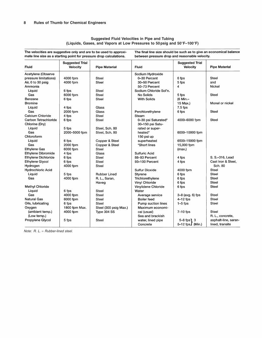
The Mak Isothermal flow chart is such a useful tool thatthe author has used it for cases where P1 is known insteadof P2 with a trial and error approach. The author has nowgenerated a graph (Figure 2) based upon M1 using Equa-tion 2. The Isothermal flow chart (Figure 1) based on M2

uses Equation 4. Figure 2 facilitates the following case.

Given: P1 and WFind: P2

Steps: 1. Get f from GPSA graph (Figure 4).2. Determine fL/D.3. Obtain Z. Figures 5, 6, and 7 are provided

for convenience.4. Calculate M1. See Equation 1.5. Get P2/P1 from Figure 2. The critical curve

indicates where M1 = P2/P1. When thishappens M2 = 1 since M2 = M1(P1/P2). Thedesign pipe diameter might have to bechanged to provide a possible set ofconditions.

6. Calculate P2.

Some calculations require knowing the critical pres-sure at which sonic velocity occurs. This is calculatedwith Equation 5.

The applicable equations are

Based on M1

(1)

(2)

Based on M2

(3)M W P D ZT Mw25

22 0 5

1 702 10= ¥ ( )[ ]( )-..

fL D M P P P P= ( ) - ( )[ ] - ( )1 11 2 12

1 222 ln

M W P D ZT Mw15

12 0 5

1 702 10= ¥ ( )[ ]( )-..

(4)

Critical pressure at the pipe outlet in psia

(5)

For comparison the author has generated an Excel® plot(Figure 3) using the data from Figure 2. This is for thosereaders who work with this popular spreadsheet.

Example

Given (see sketch following):

Calculate how much gas will flow to the vessel throughthe 1 in line with the normally closed hand valvefully opened.

Use the psv full open pressure of 136 psia as the vesselpressure.

The equivalent length of 200 ft includes the fullyopened hand valve.

The 1 in pipe’s inside diameter is 1.049 in.Assume Z = 1.0.

Calculations:

Note that if the DP was across a restriction orifice, sonicvelocity would occur since the DP is greater than 2 : 1 (315/136 = 2.31). However, the DP is along alength of pipe, so we will use Mak’s method.

For commercial steel pipe:

Note that if the flow were critical, M2 would be 1.

W lb hr= ¥ ¥ ¥( ) =0 28 1 039 10 5 70 1 702 30005. . . .

0 28 1 702 10 136 0 00764 1 0 520 165 0 5. . . .

.= ¥ ¥( )[ ] ( )[ ]- W

M W P D ZT MP psia

DT R

MZ given

W

W

25

22 0 5

22 2

1 702 101360 0874 0 00764460 60 520161 0

= ¥ ( )[ ][ ]== == + = ∞== ( )

-.

. .

.

.

fid in ft

P PfL D

M from Figure

== == == ( ) == ( )

0 0231 049 0 0874136 135 0 430 023 200 0 0874 52 60 28 1

2 1

2

.. .

.. . ..

P W d ZT Mcrit W= ( )( )408 2 0 5.

fL D M P P P P P P= ( )( ) - ( )[ ] - ( )1 12 1 22

2 12

1 222 ln

H7856-Ch001.qxd 7/4/05 6:44 PM

Fluid Flow 15

Figure 4. Friction factor chart.

H7856-Ch001.qxd 7/4/05 6:44 PM


Figure 5. Z factor for natural gas.

H7856-Ch001.qxd 7/4/05 6:44 PM

Fluid Flow 17

Fig

ure

6.

Z f

acto

r at

low

red

uced

pre

ssur

es.

Fig

ure

7.

Z f

acto

r fo

r ne

ar a

tmos

pher

ic p

ress

ure.

H7856-Ch001.qxd 7/4/05 6:45 PM

Compressible Flow—Long Pipelines

Equations Commonly Used for Calculating Hydraulic Datafor Gas Pipe Lines

Panhandle A.

Panhandle B.

Q T P D E

P PG h h PT Z

G L Z

b b b

avg

avg avg

avg avg

= ¥ ( ) ¥ ¥

¥- - ¥ ¥ -( ) ¥

¥¥ ¥ ¥

È

Î

ÍÍÍÍ

˘

˚

˙˙˙˙

737

0 0375

1 020 2 53

12

22 2 1

2

0 961

0 51

. .

.

..

T

Q T P D E

P PG h h PT Z

G L Z

b b b

avg

avg avg

avg avg

= ¥ ( ) ¥ ¥ ¥

- - ¥ ¥ -( ) ¥¥

¥ ¥ ¥

È

Î

ÍÍÍÍ

˘

˚

˙˙˙˙

435 87

0 0375

1 0778 2 6182

12

22 2 1

2

0 8539

0 5394

.

.

. .

.

.

T

Weymouth.

Pavg is used to calculate gas compressibility factor Z

Nomenclature for Panhandle Equations

Qb = flow rate, SCFDPb = base pressure, psiaTb = base temperature, °R

Tavg = average gas temperature, °RP1 = inlet pressure, psiaP2 = outlet pressure, psiaG = gas specific gravity (air = 1.0)L = line length, milesZ = average gas compressibilityD = pipe inside diameter, in.h2 = elevation at terminus of line, ft

P P P P P P Pavg = + - ¥( ) +[ ]2 3 1 2 1 2 1 2

Q T PP PGLTZ

D Eb b= ¥ ( ) ¥ -È

ÎÍ

˘

˚˙ ¥ ¥433 5 1

22

2 0 5

2 667.

.

.


Mw = Gas molecular weightP1,P2 = Inlet and outlet line pressures, psiaPcrit = Critical pressure for sonic velocity to occur, psiaT = Absolute temperature, °RW = Gas flow rate, lb/hrZ = Gas compressibility factor

Sources

1. Mak, Henry Y., “New Method Speeds Pressure-ReliefManifold Design,” Oil and Gas Journal, Nov. 20,1978, p. 166.

2. API Recommended Practice 520, “Sizing, Selection,and Installation of Pressure Relieving Devices IRefineries,” 1993.

3. “Flow of Fluids through Valves, Fittings, and Pipe,”Crane Co. Technical paper 410, 1981.

4. Crocker, Sabin, Piping Handbook, McGraw-Hill, Inc.,1945.

5. Standing, M.B. and D. L. Katz, Trans. AIME, 146, 159(1942).

NC

1in

C1

200 equiv. ft

300 psig = 315 psia60 °F

60 °F100 psig

15 psia

psv set @ 110 psig ¥ 1.1 accumulation = 121 psig = 136 psia

Example sketch

Nomenclature

D = Pipe diameter, ftd = Pipe diameter, inf = Moody friction factorL = Line equivalent length, ftM1,M2 = Mach number at the line inlet, outlet

H7856-Ch001.qxd 7/4/05 6:45 PM

Fluid Flow 19

Panhandle A.

Qb = 16,577 MCFD

Panhandle B.

Qb = 17,498 MCFD

Weymouth.

Q = 11,101 MCFD

Source

Pipecalc 2.0, Gulf Publishing Company, Houston,Texas. Note: Pipecalc 2.0 will calculate the compressibil-ity factor, minimum pipe ID, upstream pressure, down-stream pressure, and flow rate for Panhandle A, PanhandleB, Weymouth, AGA, and Colebrook-White equations.The flow rates calculated in the above sample calculationswill differ slightly from those calculated with Pipecalc 2.0since the viscosity used in the examples was extractedfrom Reference 2. Pipecalc uses the Dranchuk et al.method for calculating gas compressibility.

Q = ¥ ( ) ¥ ( ) - ( )[¥ ¥ ¥( )] ¥ ( )

0 433 520 14 7 2 000 1 500

0 6 20 560 0 835 4 026

2 2

1 2 2 667

. . , ,

. . ..

Qb = ¥ ( ) ¥ ( ) ¥ ¥

( ) - ( ) - ¥ ¥ ¥ ( )¥

( ) ¥ ¥ ¥

È

Î

ÍÍÍÍ

˘

˚

˙˙˙˙

737 520 14 7 4 026 1

2 000 1 5000 0375 0 6 100 1 762

560 0 835

0 6 20 560 835

1 020 2 53

2 22

961

0 51

. .

, ,. . ,

.

. .

. .

.

.

Qb = ¥ ( ) ¥ ( ) ¥ ¥

( ) - ( ) - ¥ ¥ ¥ ( )¥

( ) ¥ ¥ ¥

È

Î

ÍÍÍÍ

˘

˚

˙˙˙˙

435 87 520 14 7 4 026 1

2 000 1 5000 0375 0 6 100 1 762

560 0 835

0 6 20 560 835

1 0788 2 6182

2 22

8539

0 5394

. . .

, ,. . ,

.

. .

. .

.

.

h1 = elevation at origin of line, ftPavg = average line pressure, psia

E = efficiency factorE = 1 for new pipe with no bends, fittings, or pipe

diameter changesE = 0.95 for very good operating conditions, typically

through first 12–18 monthsE = 0.92 for average operating conditionsE = 0.85 for unfavorable operating conditions

Nomenclature for Weymouth Equation

Q = flow rate, MCFDTb = base temperature, °RPb = base pressure, psiaG = gas specific gravity (air = 1)L = line length, milesT = gas temperature, °RZ = gas compressibility factorD = pipe inside diameter, in.E = efficiency factor. (See Panhandle nomenclature for

suggested efficiency factors)

Sample Calculations

Q = ?G = 0.6T = 100°FL = 20 milesP1 = 2,000psiaP2 = 1,500psia

Elev diff. = 100ftD = 4.026-in.Tb = 60°FPb = 14.7psiaE = 1.0

Pavg = 2/3(2,000 + 1,500 - (2,000 ¥ 1,500/2,000 + 1,500))

= 1,762psia

Z at 1,762psia and 100°F = 0.835.

H7856-Ch001.qxd 7/4/05 6:45 PM


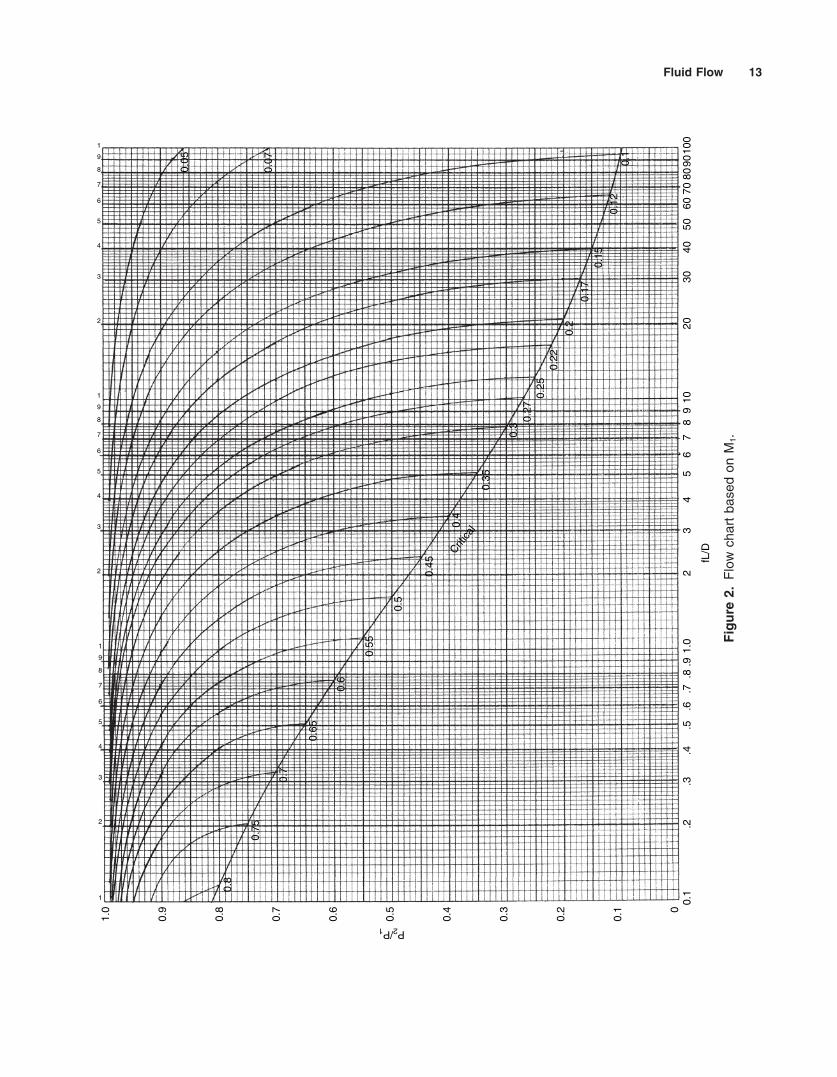
Equivalent Lengths for Multiple Lines Based on Panhandle A

Condition I.A single pipe line which consists of two or more dif-

ferent diameter lines.

Let LE = equivalent lengthL1, L2, . . . Ln = length of each diameterD1, D2, . . . Dn = internal diameter of each separate

line corresponding to L1, L2, . . .Ln

DE = equivalent internal diameter

Example. A single pipe line, 100 miles in length con-sists of 10 miles 103/4-in. OD; 40 miles 123/4-in. OD and50 miles of 22-in. OD lines.

Find equivalent length (LE) in terms of 22-in. OD pipe.

= 50 + 614 + 364= 1,028 miles equivalent length of 22-in. OD

Condition II.A multiple pipe line system consisting of two or

more parallel lines of different diameters and differentlengths.

Let LE = equivalent lengthL1, L2, L3, . . . Ln = length of various looped sectionsd1, d2, d3, . . . dn = internal diameter of the individ-

ual line corresponding to lengthL1, L2, L3 & Ln

Let LE = equivalent lengthL1, L2, L3 & Ln = length of various looped sections

L Ld

d d d d

Ld

d d d d

EE

n

nE

n

=+ + +

È

ÎÍ

˘

˚˙

+

+ + +

È

ÎÍ

˘

˚˙

1

2 6182

12 6182

22 6182

32 6182 2 6182

1 8539

2 6182

12 6182

22 6182

32 6182 2 6182

1 8539

.

. . . .

.

.

. . . .

.

. . .

. . .

. . .

LE = + ÈÎÍ

˘˚̇

+ ÈÎÍ

˘˚̇

50 4021 5

12 2510

21 510 25

4 8539 4 8539.

..

.

. .

L LDD

LDD

LDD

eE E

nE

n

= ÈÎÍ

˘˚̇

+ ÈÎÍ

˘˚̇

+ ÈÎÍ

˘˚̇1

1

4 8539

22

4 8539 4 8539. . .

. . .

d1, d2, d3 & dn = internal diameter of individualline corresponding to lengths L1,L2, L3 & Ln

when L1 = length of unlooped sectionL2 = length of single looped sectionL3 = length of double looped sectiondE = d1 = d2

then:

when dE = d1 = d2 = d3

then LE = L1 + 0.27664 L2 + 0.1305 L3

Example. A multiple system consisting of a 15 mile section of 3–85/8-in. OD lines and 1–103/4-in. OD line,and a 30 mile section of 2–85/8-in. lines and 1–103/4-in. ODline.

Find the equivalent length in terms of single 12-in. IDline.

= 5.9 + 18.1= 24.0 miles equivalent of 12-in. ID pipe

Example. A multiple system consisting of a single 12-in. ID line 5 miles in length and a 30 mile section of3–12-in. ID lines.

Find equivalent length in terms of a single 12-in. IDline.

LE =( ) +

È

ÎÍ

˘

˚˙

+( ) +

È

ÎÍ

˘

˚˙

1512

3 7 981 10 02

3012

2 7 981 10 02

2 6182

2 6182 2 6182

1 8539

2 6182

2 6182 2 6182

1 8539

.

. .

.

.

. .

.

. .

. .

L L L Ld

d dE = + +

+

È

ÎÍ

˘

˚˙1 2 3

12 6182

12 6182

32 6182

1 8539

0 276642

..

. .

.

L Ld

d d d d

Ld

d d d d

EE

n

nE

n

=+ + +

È

ÎÍ

˘

˚˙

+

+ + +

È

ÎÍ

˘

˚˙

1

2 6182

12 6182

22 6182

32 6182 2 6182

1 8539

2 6182

12 6182

22 6182

32 6182 2 6182

1 8539

.

. . . .

.

.

. . . .

.

. . .

. . .

. . .

H7856-Ch001.qxd 7/4/05 6:45 PM

Fluid Flow 21

2. McAllister, E. W., Pipe Line Rules of Thumb Handbook,3rd Ed., Gulf Publishing Co., pp. 247–248, 1993.

3. Branan, C. R., The Process Engineer’s Pocket Hand-book, Vol. 1, Gulf Publishing Co., p. 4, 1976.

LE = 5 + 0.1305 ¥ 30= 8.92 miles equivalent of single 12-in. ID line

References

1. Maxwell, J. B., Data Book on Hydrocarbons, Van Nostrand, 1965.

Sonic Velocity

To determine sonic velocity, use

where

Vs = Sonic velocity, ft/secK = Cp/Cv the ratio of specific heats at constant pressure

to constant volume. This ratio is 1.4 for mostdiatomic gases.

g = 32.2ft/sec2

R = 1,544/mol. wt.T = Absolute temperature in °R

V KgRTs =

To determine the critical pressure ratio for gas sonicvelocity across a nozzle or orifice use

If pressure drop is high enough to exceed the critical ratio,sonic velocity will be reached. When K = 1.4, ratio =0.53.

Source

Branan, C. R., The. Process Engineer’s Pocket Hand-book, Vol. 1, Gulf Publishing Co., 1976.

critical pressure ratio Kk k

= +( )[ ] -( )2 1

1

Metering

Orifice

Permanent head loss % of DhPermanent

Do/Dp Loss0.2 950.4 820.6 630.8 40

One designer uses permanent loss = Dh (1 - Co)

where

Uo = Velocity through orifice, ft/secUp = Velocity through pipe, ft/sec

U U C g ho p o2 2 1 2 1 2

2-( ) = ( )D

2g = 64.4ft/sec2

Dh = Orifice pressure drop, ft of fluidD = DiameterCo = Coefficient. (Use 0.60 for typical application where

Do/Dp is between 0.2 and 0.8 and Re at vena con-tracta is above 15,000.)

Venturi

Same equation as for orifice:

Co = 0.98

Permanent head loss approximately 3–4% Dh.

H7856-Ch001.qxd 7/4/05 6:45 PM


Pitot Tube

Source

Branan, C. R., The Process Engineer’s Pocket HandbookVol. 1, Gulf Publishing Co., 1976.

Dh u g= 2 2

Rectangular Weir

where

FV = Flow in ft3/secL = Width of weir, ftH = Height of liquid over weir, ft

F L H Hv = -( )3 33 0 2 3 2. .

where

DPallow = Maximum allowable differential pressure forsizing purposes, psi

Km = Valve recovery coefficient (see Table 3)rc = Critical pressure ratio (see Figures 1 and 2)

P1 = Body inlet pressure, psiaPv = Vapor pressure of liquid at body inlet tempera-

ture, psia

This gives the maximum DP that is effective in produc-ing flow. Above this DP no additional flow will be pro-duced since flow will be restricted by flashing. Do not usea number higher than DPallow in the liquid sizing formula.

Notes:

1. References 1 and 2 were used extensively for thissection. The sizing procedure is generally that ofFisher Controls Company.

2. Use manufacturers’ data where available. This hand-book will provide approximate parameters applicableto a wide range of manufacturers.

3. For any control valve design be sure to use one ofthe modern methods, such as that given here, thattakes into account such things as control valve pres-sure recovery factors and gas transition to incom-pressible flow at critical pressure drop.

Liquid Flow

Across a control valve the fluid is accelerated to some maximum velocity. At this point the pressurereduces to its lowest value. If this pressure is lower thanthe liquid’s vapor pressure, flashing will produce bubblesor cavities of vapor. The pressure will rise or “recover”downstream of the lowest pressure point. If the pressurerises to above the vapor pressure, the bubbles or cavitiescollapse. This causes noise, vibration, and physicaldamage.

When there is a choice, design for no flashing. Whenthere is no choice, locate the valve to flash into a vesselif possible. If flashing or cavitation cannot be avoided,select hardware that can withstand these severe condi-tions. The downstream line will have to be sized for twophase flow. It is suggested to use a long conical adaptorfrom the control valve to the downstream line.

When sizing liquid control valves first use

DP K P r Pallow m c v= -( )1

Figure 1. Enter on the abscissa at the water vapor pres-sure at the valve inlet. Proceed vertically to intersect thecurve. Move horizontally to the left to read rc on the ordi-nate (Reference 1).

Control Valves

H7856-Ch001.qxd 7/4/05 6:45 PM

Fluid Flow 23

Gas and Steam Flow

The gas and steam sizing formulas are Gas

CQ

GTP

CP

P

g =ÈÎÍ

˘˚̇

520 34171

1 1

sindeg.

DSome designers use as the minimum pressure for flashcheck the upstream absolute pressure minus two timescontrol valve pressure drop.

Table 1 gives critical pressures for miscellaneousfluids. Table 2 gives relative flow capacities of varioustypes of control valves. This is a rough guide to use inlieu of manufacturer’s data.

The liquid sizing formula is

where

Cv = Liquid sizing coefficientQ = Flow rate in GPM

DP = Body differential pressure, psiG = Specific gravity (water at 60°F = 1.0)

Two liquid control valve sizing rules of thumb are

1. No viscosity correction necessary if viscosity �20centistokes.

2. For sizing a flashing control valve add the Cv’s ofthe liquid and the vapor.

C QGP

v =D

Figure 2. Determine the vapor pressure/critical pressureratio by dividing the liquid vapor pressure at the valve inletby the critical pressure of the liquid. Enter on the abscissaat the ratio just calculated and proceed vertically to inter-sect the curve. Move horizontally to the left and read rc

on the ordinate (Reference 1).

Table 1Critical Pressure of Various Fluids, Psia*

Table 2Relative Flow Capacities of Control Valves (Reference 2)

*For values not listed, consult an appropriate reference book.

Note: This table may serve as a rough guide only since actual flowcapacities differ between manufacturer’s products and individual valvesizes. (Source: ISA “Handbook of Control Valves” Page 17).*Valve flow coefficient Cv = Cd ¥ d2 (d = valve dia., in.).†Cv/d2 of valve when installed between pipe reducers (pipe dia. 2 ¥ valvedia.).**Cv/d2 of valve when undergoing critical (choked) flow conditions.

H7856-Ch001.qxd 7/4/05 6:45 PM


G = Gas specific gravity = mol. wt./29P1 = Valve inlet pressure, psia

DP = Pressure drop across valve, psiQ = Gas flow rate, SCFHQs = Steam or vapor flow rate, lb/hrT = Absolute temperature of gas at inlet, °R

Tsh = Degrees of superheat, °F

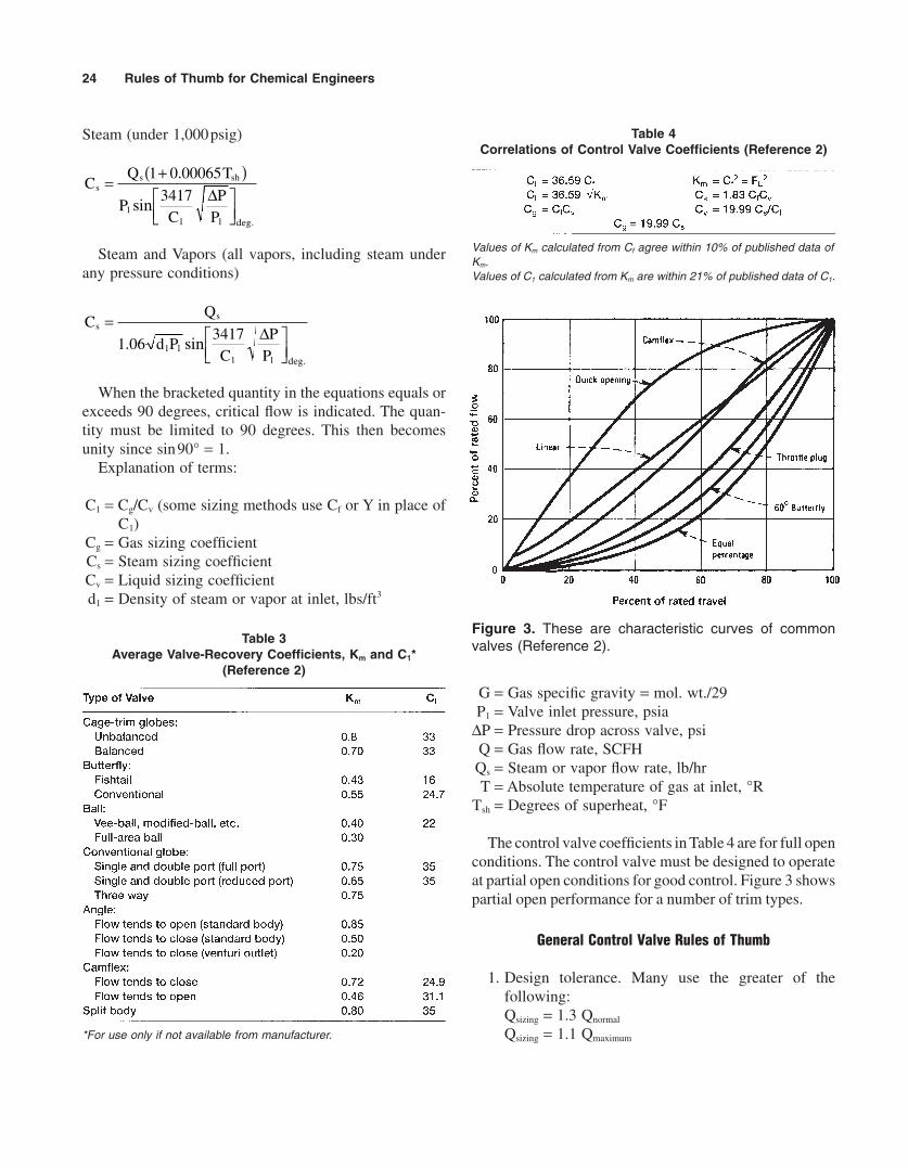
The control valve coefficients in Table 4 are for full openconditions. The control valve must be designed to operateat partial open conditions for good control. Figure 3 showspartial open performance for a number of trim types.

General Control Valve Rules of Thumb

1. Design tolerance. Many use the greater of the following:Qsizing = 1.3 Qnormal

Qsizing = 1.1 Qmaximum

Steam (under 1,000psig)

Steam and Vapors (all vapors, including steam underany pressure conditions)

When the bracketed quantity in the equations equals orexceeds 90 degrees, critical flow is indicated. The quan-tity must be limited to 90 degrees. This then becomesunity since sin90° = 1.

Explanation of terms:

C1 = Cg/Cv (some sizing methods use Cf or Y in place ofC1)

Cg = Gas sizing coefficientCs = Steam sizing coefficientCv = Liquid sizing coefficientd1 = Density of steam or vapor at inlet, lbs/ft3

CQ

d PC

PP

ss=

ÈÎÍ

˘˚̇

1 063417

1 11 1

. sindeg.

D

CQ T

PC

PP

ss sh= +( )

ÈÎÍ

˘˚̇

1 0 00065

34171

1 1

.

sindeg.

D

Figure 3. These are characteristic curves of commonvalves (Reference 2).Table 3

Average Valve-Recovery Coefficients, Km and C1*(Reference 2)

*For use only if not available from manufacturer.

Table 4Correlations of Control Valve Coefficients (Reference 2)

Values of Km calculated from Cf agree within 10% of published data ofKm.Values of C1 calculated from Km are within 21% of published data of C1.

H7856-Ch001.qxd 7/4/05 6:45 PM

Fluid Flow 25

Safety Relief Valves

The ASME code1 provides the basic requirements forover-pressure protection. Section I, Power Boilers, coversfired and unfired steam boilers. All other vessels in-cluding exchanger shells and similar pressure containingequipment fall under Section VIII, Pressure Vessels. APIRP 520 and lesser API documents supplement the ASMEcode. These codes specify allowable accumulation, whichis the difference between relieving pressure at which thevalve reaches full rated flow and set pressure at which thevalve starts to open. Accumulation is expressed as per-centage of set pressure in Table 1. The articles by Rearick2

and Isqacs3 are used throughout this section.Full liquid containers require protection from thermal

expansion. Such relief valves are generally quite small.Two examples are

1. Cooling water that can be blocked in with hot fluidstill flowing on the other side of an exchanger.

2. Long lines to tank farms that can lie stagnant andexposed to the sun.

Sizing

Use manufacturer’s sizing charts and data where avail-able. In lieu of manufacturer’s data use the formula

where

Dh = Head loss in feet of flowing fluidu = Velocity in ft/secg = 32.2ft/sec2

This will give a conservative relief valve area. Forcompressible fluids use Dh corresponding to 1/2P1 if headdifference is greater than that corresponding to 1/2P1 (sincesonic velocity occurs). If head difference is below thatcorresponding to 1/2P1 use actual Dh.

For vessels filled with only gas or vapor and exposedto fire use

(API RP 520, Reference 4)

A = Calculated nozzle area, in.2

P1 = Set pressure (psig) ¥ (1 + fraction accumulation) +atmospheric pressure, psia. For example, if accu-mulation = 10%, then (1 + fraction accumulation) =1.10

Ad = Exposed surface of vessel, ft2

AA

Ps= 0 042

1

.

u g h= 0 4 2. D

2. Type of trim. Use equal percentage whenever thereis a large design uncertainty or wide rangeability isdesired. Use linear for small uncertainty cases.

Limit max/min flow to about 10 for equal per-centage trim and 5 for linear. Equal percentage trimusually requires one larger nominal body size thanlinear.

3. For good control where possible, make the controlvalve take 50%–60% of the system flowing head loss.

4. For saturated steam keep control valve outlet veloc-ity below 0.25 mach.

5. Keep valve inlet velocity below 300ft/sec for 2≤ andsmaller, and 200ft/sec for larger sizes.

References

1. Fisher Controls Company, Sizing and Selection Data,Catalog 10.

2. Chalfin, Fluor Corp., “Specifying Control Valves,”Chemical Engineering, October 14, 1974.

Table 1Accumulation Expressed as Percentage of Set Pressure

H7856-Ch001.qxd 7/4/05 6:45 PM


Plants, situations, and causes of overpressure tend tobe dissimilar enough to discourage preparation of gener-alized calculation procedures for the rate of discharge. Inlieu of a set procedure most of these problems can besolved satisfactorily by conservative simplification andanalysis. It should be noted also that, by general assump-tion, two unrelated emergency conditions will not occursimultaneously.

The first three causes of overpressure on our list aremore amenable to generalization than the others and willbe discussed.

Fire

The heat input from fire is discussed in API RP 520(Reference 4). One form of their equation for liquid con-taining vessels is

Q = 21,000FAw0.82

where

Q = Heat absorption, Btu/hrAw = Total wetted surface, ft2

F = Environment factor

This will also give conservative results. For heat inputfrom fire to liquid containing vessels see “Determinationof Rates of Discharge.”

The set pressure of a conventional valve is affected byback pressure. The spring setting can be adjusted to com-pensate for constant back pressure. For a variable backpressure of greater than 10% of the set pressure, it is cus-tomary to go to the balanced bellows type which can gen-erally tolerate variable back pressure of up to 40% of setpressure. Table 2 gives standard orifice sizes.

Determination of Rates of Discharge

The more common causes of overpressure are

1. External fire2. Heat Exchanger Tube Failure3. Liquid Expansion4. Cooling Water Failure5. Electricity Failure6. Blocked Outlet7. Failure of Automatic Controls8. Loss of Reflux9. Chemical Reaction (this heat can sometimes exceed

the heat of an external fire). Consider bottom ventingfor reactive liquids.5

Table 2Relief Valve Designations

H7856-Ch001.qxd 7/4/05 6:45 PM

Fluid Flow 27

Liquid Expansion

The following equation can be used for sizing reliefvalves for liquid expansion.

(API RP 520, Reference 4)

where

Q = Required capacity, gpmH = Heat input, Btu/hrB = Coefficient of volumetric expansion per °F:

= 0.0001 for water= 0.0010 for light hydrocarbons= 0.0008 for gasoline= 0.0006 for distillates= 0.0004 for residual fuel oil

G = Specific gravityC = Specific heat, Btu/lb °F

Rules of Thumb for Safety Relief Valves

1. Check metallurgy for light hydrocarbons flash-ing during relief. Very low temperatures can be produced.

2. Always check for reaction force from the tailpipe.3. Hand jacks are a big help on large relief valves for

several reasons. One is to give the operator a chanceto reseat a leaking relief valve.

4. Flat seated valves have an advantage over bevelseated valves if the plant forces have to reface thesurfaces (usually happens at midnight).

5. The maximum pressure from an explosion of ahydrocarbon and air is 7 ¥ initial pressure, unless itoccurs in a long pipe where a standing wave can be set up. It may be cheaper to design some smallvessels to withstand an explosion than to provide asafety relief system. It is typical to specify 1/4≤ asminimum plate thickness (for carbon steel only).

Sources

1. ASME Boiler and Pressure Vessel Code, Sections Iand VIII.

2. Rearick, “How to Design Pressure Relief Systems,”Parts I and II, Hydrocarbon Processing, August/September 1969.

QBH

GC=

500

The environmental factors represented by F are

Bare vessel = 1.0Insulated = 0.3/insulation thickness, in.Underground storage = 0.0Earth covered above grade = 0.03

The height above grade for calculating wetted surfaceshould be

1. For vertical vessels—at least 25 feet above grade orother level at which a fire could be sustained.

2. For horizontal vessels—at least equal to themaximum diameter.

3. For spheres or spheroids—whichever is greater, theequator or 25 feet.

Three cases exist for vessels exposed to fire as pointedout by Wong.6 A gas filled vessel, below 25ft (flameheights usually stay below this), cannot be protected bya PSV alone. The metal wall will overheat long before thepressure reaches the PSV set point. Wong discusses anumber of protective measures. A vessel containing ahigh boiling point liquid is similar because very littlevapor is formed at the relieving pressure, so there is verylittle heat of vaporization to soak up the fire’s heat input.

A low-boiling-point liquid, in boiling off, has a goodheat transfer coefficient to help cool the wall and buytime. Calculate the time required to heat up the liquid andvaporize the inventory. If the time is less than 15 minutestreat the vessel as being gas filled. If the time is more than15–20 minutes treat it as a safe condition. However, inthis event, be sure to check the final pressure of the vesselwith the last drop of liquid for PSV sizing.

Heat Exchanger Tube Failure

1. Use the fluid entering from twice the cross sectionof one tube as stated in API RP 5204 (one tube cutin half exposes two cross sections at the cut).4

2. Use Dh = u2/2g to calculate leakage. Since this actssimilar to an orifice, we need a coefficient; use 0.7.So,

For compressible fluids, if the downstream head is lessthan 1/2 the upstream head, use 1/2 the upstream head as Dh.Otherwise use the actual Dh.

u g h= 0 7 2. D

H7856-Ch001.qxd 7/4/05 6:45 PM


5. Walter, Y. L. and V. H. Edwards,” Consider BottomVenting for Reactive Liquids,” Chemical EngineeringProgress, June 2000, p. 34.

6. Wong, W. Y., “Improve the Fire Protection of PressureVessels,” Chemical Engineering, October, 1999, p.193.

3. Isaacs, Marx, “Pressure Relief Systems,” ChemicalEngineering, February 22, 1971.

4. Recommended Practice for the Design and Installationof Pressure Relieving Systems in Refineries, Part I—“Design,” latest edition, Part II—“Installation,” latestedition RP 520 American Petroleum Institute.

H7856-Ch001.qxd 7/4/05 6:45 PM

SECTION ONE Equipment Design

Documents

Transcript of SECTION ONE Equipment Design