Section 8.3 - A Confidence Interval for the Difference of Two Proportions Objectives: 1.To find the...
27
Section 8.3 - A Confidence Interval for the Difference of Two Proportions Objectives: • To find the mean and standard error of the sampling distribution for the difference of two proportions. • To construct and interpret a confidence interval for the difference of two proportions.
-
Upload
marilyn-kennedy -
Category
Documents
-
view
215 -
download
1
Transcript of Section 8.3 - A Confidence Interval for the Difference of Two Proportions Objectives: 1.To find the...

Section 8.3 - A Confidence Interval for the Difference of Two Proportions
Objectives:
• To find the mean and standard error of the sampling distribution for the difference of two proportions.
• To construct and interpret a confidence interval for the difference of two proportions.

Introduction
A recent poll of 29,700 U.S. households found that 63% owned a pet. The percentage in 1994 was 56%.
What was the change in the percentage of U.S. households that own a pet?
Section 8.3 - A Confidence Interval for the Difference of Two Proportions

Introduction
A recent poll of 29,700 U.S. households found that 63% owned a pet. The percentage in 1994 was 56%.
What was the change in the percentage of U.S. households that own a pet?
The obvious answer, that the percentage increased by 7 percentage points, is only an estimate because 7% is the difference of two sample percentages. These sample percentages, 56% and 63%, are probably not equal to the population percentages.
We would like to find a confidence interval and margin of error to go with the difference of 7%.
Section 8.3 - A Confidence Interval for the Difference of Two Proportions

The Formula for the Confidence Interval
Section 8.3 - A Confidence Interval for the Difference of Two Proportions
A confidence interval for the difference of the two proportions,
p1 −p2 , has the form: p1 −p2( )±z* ⋅SEp1−p2
What is the standard error of the difference?

The Formula for the Confidence Interval
Section 8.3 - A Confidence Interval for the Difference of Two Proportions
Let p1 and p2 be the two population proportions.
Let p1 and p2 be the two sample proportions.
We are interested in the random variable that is the difference
of the two sample proportions : p1 −p2
From Section 6.1, we know that (1) the mean of the difference is equal to the difference of the means, and (2), if the variablesare independent, the variance of the difference is equal to thesum of the variances : μ p1−p2
=μ p1−μ p2
σ p1−p22 =σ p1
2 +σ p22 ⇒ σ p1−p2
= σ p12 +σ p2
2

The Formula for the Confidence Interval
Section 8.3 - A Confidence Interval for the Difference of Two Proportions
The two means are μ p1= p1 and μ p2
= p2 , so μ p1− p2= p1 − p2 .
The two standard errors are σ p1
2 =p1(1− p1)
n1
and
σ p2
2 =p2 (1− p2 )
n2
where n1 and n2 are the two sample sizes.
We can estimate these two standard errors by
p1(1− p1)n1
and p2 (1− p2 )
n2
and we can estimate the standard error of the difference by
σ p1− p2=
p1(1− p1)n1
+p2 (1− p2 )
n2

Confidence Interval for the Difference of Two Proportions
Section 8.3 - A Confidence Interval for the Difference of Two Proportions
Let p1 and p2 be the proportions of successes in two random
samples of size n1 and n2 , respectively. (The sample sizes do
not have to be equal.)
The confidence interval for the difference, p1 −p2 ,of the proportion of successes in the two populations is
p1 −p2( ) ±z*p1(1−p1 )
n1+p2 (1−p2 )
n2
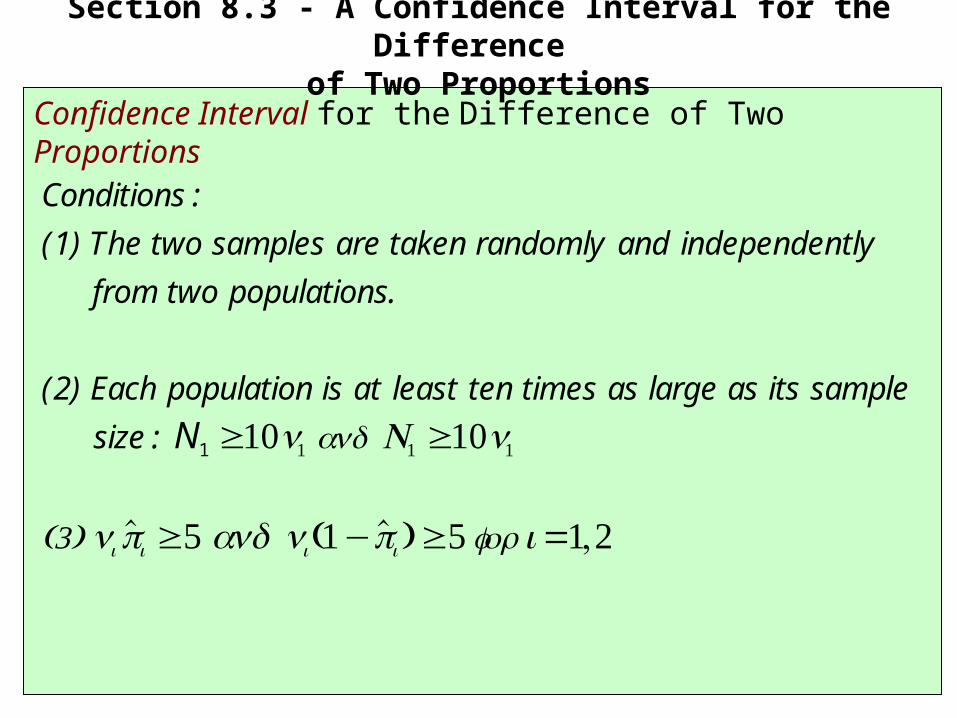
Confidence Interval for the Difference of Two Proportions
Section 8.3 - A Confidence Interval for the Difference of Two Proportions
Conditions :
(1) The two samples are taken randomly and independently
from two populations.
(2) Each population is at least ten times as large as its sample
size: N1 ≥10n1 and N1 ≥10n1
(3) ni pi ≥5 and ni (1−pi )≥5 for i=1,2

E50. The USC Annenberg School Center for the Digital Future found that 66.9% of Americans used the Internet in 2000 and 78.6% used the Internet in 2005. Assume that the samples were independently and randomly selected and that the sample size was 2000 in both years.
• Check the conditions for constructing a confidence interval for the difference of two proportions.
• Find a 99% confidence interval for the difference of proportions.
• Interpret the resulting interval in the context of the problem.
• Is 0 in the confidence interval? What does your answer imply?
Section 8.3 - A Confidence Interval for the Difference of Two Proportions

E50a. The USC Annenberg School Center for the Digital Future found that 66.9% of Americans used the Internet in 2000 and 78.6% used the Internet in 2005. Assume that the samples were independently and randomly selected and that the sample size was 2000 in both years.
Section 8.3 - A Confidence Interval for the Difference of Two Proportions
Conditions :
(1) The two samples are taken randomly and independently
from the two populations.
(2) The population in 2000 and 2005 was at least 10n = 20,000
(3) n2000 p2000 =(2000)(0.669) =1338≥5; n2000 (1−p2000 )=662 ≥5 n2005 p2005 =(2000)(0.786) =1572≥5; n2000 (1−p2000 )=428 ≥5

E50b. The USC Annenberg School Center for the Digital Future found that 66.9% of Americans used the Internet in 2000 and 78.6% used the Internet in 2005. Assume that the samples were independently and randomly selected and that the sample size was 2000 in both years.
Section 8.3 - A Confidence Interval for the Difference of Two Proportions
The 99% confidence interval for the difference, p2005 −p2000 :
p1 −p2( ) ±z*p1(1−p1 )
n1+p2 (1−p2 )
n2
= 0.7861 −0.669( ) ±2.576(0.786)(0.214)
2000+(0.669)(0.331)
2000
=0.117 ±0.036
= 0.081, 0.153[ ]

E50c. The USC Annenberg School Center for the Digital Future found that 66.9% of Americans used the Internet in 2000 and 78.6% used the Internet in 2005. Assume that the samples were independently and randomly selected and that the sample size was 2000 in both years.
We are 99% confident that the difference between the proportion of Americans who used the Internet in 2005 and the proportion who used the Internet in 2000 is between 8.1% and 15.3%.
We are 99% confident that the interval from 0.081 to 0.153 contains the difference in the proportions of Americans who used the Internet in 2005 and 2000.
Section 8.3 - A Confidence Interval for the Difference of Two Proportions

E50d. The USC Annenberg School Center for the Digital Future found that 66.9% of Americans used the Internet in 2000 and 78.6% used the Internet in 2005. Assume that the samples were independently and randomly selected and that the sample size was 2000 in both years.
No, 0 is not in the interval [0.081, 0.153].
The proportions in 2000 and 2005 were different.
We are 99% confident that the proportion of Americans who used the Internet increased from 2000 to 2005.
Section 8.3 - A Confidence Interval for the Difference of Two Proportions

Objectives:
1. To use simulation to construct an approximate sampling distribution for the difference of two proportions
2. To review the sampling distribution for the difference of two proportions when p1 = p2.
3. To use a test of significance to decide whether to reject a claim that two samples were drawn from two binomial populations that have the same proportion of successes.
Section 8.4 - A Significance Test for the Difference of Two Proportions

Introduction
In Section 8.3, we extended our knowledge of confidence intervals and sampling distributions and learned how to compute a confidence interval for the difference of two proportions.
We will now extend our knowledge of tests of significance to differences of two proportions.
We want to be able to determine if an observed difference can reasonably be attributed to chance, or if the observed difference is large enough to be able to rule out chance as a likely explanation.
Section 8.4 - A Significance Test for the Difference of Two Proportions

The Test Statistic
Section 8.4 - A Significance Test for the Difference of Two Proportions
test statistic =statistic−parameter
standard deviation of statisticstatistic= p1 −p2
parameter =p1 −p2
standard error =p1(1−p1 )
n1+p2 (1−p2 )
n2

The Test Statistic
Section 8.4 - A Significance Test for the Difference of Two Proportions
In order to compute the standard error, we need estimates of p1 and p2 .
We could estimate p1 and p 2 by p1 and p 2 , respectively.
However, under the null hypothesis p = p1 = p 2 .
We can estimate p = p1 = p2 by combining the data from both samples
into a pooled estimate, p :
p=p1n1 + p2n2n1 +n2
Note that the pooled estimate is a weighted average of the two sampleproportions.Another way to think of the pooled estimate is
p=total number of successes in both samplestotal sample size

The Test Statistic
Section 8.4 - A Significance Test for the Difference of Two Proportions
standard error =p1(1−p1 )
n1+p2 (1−p2 )
n2
=p(1−p)
n1+p(1−p)
n2
= p(1−p)1n1
+1n2
⎛
⎝⎜⎞
⎠⎟

The Test Statistic
Section 8.4 - A Significance Test for the Difference of Two Proportions
test statistic =statistic−parameter
standard error
z=p1 −p2( )− p1 −p2( )
p(1−p)1n1
+1n2
⎛
⎝⎜⎞
⎠⎟

The USC Annenberg School Center for the Digital Future found that 66.9% of Americans used the Internet in 2000 and 78.6% used the Internet in 2005. Assume that the samples were independently and randomly selected and that the sample size was 2000 in both years.
Test the claim that the proportion of Americans using the Internet increased between 2000 and 2005. Use a significance level of = 0.01.
Section 8.4 - A Significance Test for the Difference of Two Proportions

Check conditions for inference.
Section 8.3 - A Significance Test for the Difference of Two Proportions
We are conducting a significance test for the difference
of two proportions, with = 0.01
Conditions :(1) The two samples are taken randomly and independently from the two populations.
(2) The population in 2000 and 2005 was at least 10n = 20,000
(3) n2000 p2000 = (2000)(0.669) = 1338 ≥ 5; n2000 (1− p2000 ) = 662 ≥ 5
n2005 p2005 = (2000)(0.786) = 1572 ≥ 5; n2000 (1− p2000 ) = 428 ≥ 5

Write a null and alternative hypothesis.
Section 8.4 - A Significance Test for the Difference of Two Proportions
Claim: the proportion of Americans using the Internet increased
from 2000 to 2005.
Opposite claim: The proportion of Americans using the Internet
did not increase between 2000 and 2005.
Let p2000 and p2005 represent the proportion of Americans using
the Internet in 2000 and 2005, respectively.
Claim : p2005 > p2000Opposite claim: p2005 ≤p2000
H0 : p2005 −p2000 =0 This is a right - tailed test.H1 : p2005 −p2000 > 0 =0.01 is placed in the right tail.

Compute the test statistic.
Section 8.4 - A Significance Test for the Difference of Two Proportions
p2000 =0.669; n2000 =2000p2005 =0.786; n2005 =2000
p=1338 +15722000 + 2000
=0.7275
z=p2005 −p2000( )− p2005 −p2000( )
p(1−p)1
n2005
+1
n2000
⎛
⎝⎜⎞
⎠⎟
=0.786 −0.669( )− 0( )
(0.7275)(0.2725)1
2000+
12000
⎛⎝⎜
⎞⎠⎟
=8.31

Compute the P-value.
Section 8.4 - A Significance Test for the Difference of Two Proportions
P −value=P(z≥8.31)=1−P(z≤8.31)=0.0001

Determine the critical value.
Section 8.4 - A Significance Test for the Difference of Two Proportions
Right - tailed test with =0.01⇒ area of 0.01 in the right tail⇒ area of 0.9900 to the left of the critical value [2ND VARS] DISTR 3 invNorm(.99) 2.326347877
⇒ z* =2.33

Write a conclusion.
Critical value method:
Because the test statistic z = 8.31 falls to the right of the critical value z* = 2.33, we reject the null hypothesis that
p2005 - p2000 = 0 at the = 0.01 level.
P-value method:
Because the P-value of 0.0001 is less than the significance level 0.01, we reject the null hypothesis that p2005 - p2000 = 0 at the = 0.01 level.
Section 8.4 - A Significance Test for the Difference of Two Proportions

Write a conclusion.
We conclude that there is sufficient sample evidence to support the claim that the proportion of Americans who use the Internet has increased between 2000 to 2005.
Section 8.4 - A Significance Test for the Difference of Two Proportions