SECTION 8: RELIABILITY DATA COLLECTION AND ANALYSIS ...

MIL-HDBK-338B

SECTION 8: RELIABILITY DATA COLLECTION AND ANALYSIS,DEMONSTRATION, AND GROWTH

8-170

• Highly Accelerated Stress Screens (HASS) (Equipment-level)• Highly Accelerated Temperature and Humidity Stress Test (HAST) (Part-level)

Highly accelerated testing is the systematic application of environmental stimuli at levels wellbeyond those anticipated during product use. Thus, the results need to be carefully interpreted. Itis used to identify relevant faults and to assure that the resulting products have a sufficientmargin of strength above that required to survive the normal operating environments. Highlyaccelerated testing attempts to greatly reduce the time needed to precipitate these defects. Theapproach may be used either for development testing or for screening.

HALT is a development tool and HASS is a screening tool. They are frequently employed inconjunction with one another. They are new, and are in conflict with the classical approach toaccelerated testing; thus, they are controversial. Their specific goal, however, is to improve theproduct design to a point where manufacturing variations and environment effects have minimalimpact on performance and reliability. There is usually no quantitative life or reliabilityprediction associated with highly accelerated testing.

8.7.6.1 Step Stress Profile Testing

Using a step stress profile, test specimens are subjected to a given level of stress for a presetperiod of time, then they are subjected to a higher level of stress for a subsequent period of time.The process continues at ever increasing levels of stress, until either; all specimens fail, or thetime period at the maximum level stress ends, as shown in Figure 8.7-2. This approach providesmore rapid failures for analysis, but with this technique it is very difficult to properly model theacceleration and hence to quantitatively predict the item life under normal usage.

Stress

Time

FIGURE 8.7-2: STEP STRESS PROFILE

中国可靠性网 http://www.kekaoxing.com

http://www.kekaoxing.com

MIL-HDBK-338B


8-171

How much to increase the stress in any single step is a function of many variables and is beyondthe scope of this discussion. However, the general rule to follow in the design of such a test is toeventually exceed the expected environments by a comfortable margin so that all members of thepopulation can be expected to survive both the field environment and the screen environments,assuming of course that they are defect free.

8.7.6.2 Progressive Stress Profile Testing

A progressive stress profile or “ramp test” is another frequently used approach (see Figure 8.7-3).With this approach the level of stress is continuously increased with time. The advantages anddisadvantages are the same as those for step stress testing, but with the additional difficulty ofaccurately controlling the rate of increase, of the stress.

FIGURE 8.7-3: PROGRESSIVE STRESS PROFILE

8.7.6.3 HALT Testing

The term HALT was coined in 1988 by Gregg K. Hobbs (Ref. [8]). HALT (also, sometimesreferred to as STRIFE (Stress plus Life) testing) is a development test, an enhanced form of stepstress testing. It is typically used to identify design weaknesses and manufacturing processproblems and to increase the margin of strength of the design rather than to predict quantitativelife or reliability of the product.

HALT testing begins with step stress testing in generic stresses such as temperature, rate ofchange of temperature, vibration, voltage, power cycling and humidity. In addition, productunique stresses such as clock frequency, DC voltage variation and even component valuevariation may be the accelerated stimuli.

Stress

Time

MIL-HDBK-338B


8-172

The type of the vibration stimuli used for HALT (and HASS) testing is unique. It is not basedupon the universally accepted accelerated (power) spectral density concept. Thus it does notutilize classical, single-axis, sinusoidal vibration or a random vibration spectrum, generated byacceleration-controlled electro-dynamic shakers. Instead an unconventional multi-axialpneumatic (six degree of freedom) impact exciter is typically used. This type of equipmentgenerates a highly unique broadband accelerated shock response spectrum (SRS). This iseffectively a repeated shock environment rather than a vibration environment and is, in its self,much more severe than a classical vibration spectrum. Because of the choice of this shock stimulispectrum, the resulting data cannot be easily correlated with either: (a) the normal environmentor with (b) classical vibration testing using classical vibration modeling approaches. Thusquantitative prediction of life or reliability is not usually possible with HALT and HASS.

Using HALT the step stress process continues until stress levels well above those expected in thenormal operational environments are exceeded. Throughout the process continuous evaluation isperformed to determine how to make the unit able to withstand the increasing stress. Generallytemporary fixes are implemented just so that the test can continue. When a group of fixes isidentified, a permanent block change is then implemented.

After one stimuli has been elevated to a level felt to be sufficient, another stimuli is selected forstep stress testing. This progression continues until all stimuli have been applied separately.Then combined stresses are run to exploit the synergism between the stresses, that is, thecombined effect may generate larger stresses than either stress alone would create. After designfixes for the identified problems have been implemented, a second series of step stresses are runto verify the fixes, assure that the fixes themselves have not introduced new problems and to lookfor additional problems which may have been missed due to the limited sample size. This aspectof HALT must be taken into account in selecting the appropriate stress levels since a slightincrease in stress can greatly reduce the number of cycles to failure.

For all of these stimuli, the upper and lower operating limits and the destruct limits should befound or at least understood. Understood means that although the limits are not actually found,they are verified to be well beyond the limits which may be used in any future HASS test andeven farther beyond the normal field environments. For example, a product may be able to

withstand an hour of random vibration at 20 Grms without failure. Although the destruct limitmay not have been found, it is certainly high enough for most commercial equipment intended

for non-military environments where the screen environment may be 10 Grms random vibrationfor 5 minutes and the worst field environment is a truck ride while in an isolation container. Thisexample of the capability far exceeding the field environment is quite common when HALT isproperly applied.

There are several reasons for ascertaining both the operating limits and the destruct limits.Knowledge of the operating limits is necessary in order to assess if suitable design margins existand how large the margins are likely to be as a function of population. It is also necessary toformulate failure detection tests. These can be run during any future HASS test since the



MIL-HDBK-338B


8-173

detection tests run during stimulation are necessary for high detectability of precipitated defects.Knowledge of the destruct limits is required in order to determine the design margins in non-operating environments and to assure that any future HASS environments are well below destructlevels.

8.7.6.4 HASS Testing

HASS is a form of accelerated environmental stress screening. It presents the most intenseenvironment of any seen by the product, but it is typically of a very limited duration. HASS isdesigned to go to “the fundamental limits of the technology.” This is defined as the stress levelat which a small increase in stress causes a large increase in the number of failures. An exampleof such a fundamental limit might be the softening point of plastics.

HASS requires that the product have a sufficient margin of strength above that required tosurvive the normal use environments. Temperature, vibration levels, voltage and other stimuliexceeding the normal levels are used in HASS to force rapid defect precipitation in order to makethe screens more effective and economical. The use of HASS requires a thorough knowledge ofthe product’s ability to function at the extended ranges of simulation and also detailed knowledgeabout the failure mechanisms which limit these stimuli levels. Design and process changes areusually made to extend the functional and destruct levels of the equipment in order to assurelarge design and process margins as well as to allow HASS, with its attendant cost savings, to beperformed. These saving can potentially produce orders of magnitude reduction in screening costas well as significant quality improvements. One risk is that the item may be overdesigned.

Development of screening levels to be used in HASS begins during HALT testing. Operationallevels and destruct levels are used as guidelines to select environmental limits during HASS.Two levels of environmental stimuli are chosen for each accelerated screening environment: theprecipitation level and the detection level. Precipitation is the manifestation of a latent, ordormant, product flaw (i.e., it changes from a latent state to a patent or evident, detectable state).Detection is the observation that an abnormality exists. The observation may be made visually,electronically, audibly, etc.

The precipitation levels are chosen to be well below the destruct level, but beyond theoperational limits. During the precipitation screen, the test item may not operate within therequired limits but functional operation must be maintained and it must be monitored. Theselevels serve as the acceleration factor to minimize the time necessary to precipitate faults. Thedetection stress level is chosen outside of or just below the operational level determined duringHALT testing. During the detection portion of the screen, operational parameters are monitoredfor compliance with the requirements. Once the screening parameters have been set, a proof-of-screen test must be performed to ensure that the accelerated screening levels are not damagingthe product. The proof-of-screen is performed by simply running multiply accelerated screeningprofiles until either the product wears out or assurance is gained that the screen is not devouringappreciable useful life. Typically, repeating the screening environment 10 times is acceptable

MIL-HDBK-338B


8-174

proof, provided there is no evidence of product wear out.

Its is critical that the product be powered up and monitored during HASS. A large portion,typically greater than 50%, of the faults identified during screening are soft or intermittent faults.Not having complete diagnostics and detection these faults can be disastrous. An intermittentfault in the factory is very likely to be an early failure in the field.

HASS is a time compressed environmental stress screen applied at the earliest functional level ofassembly. Complete functional monitoring of the test item is extremely important. Non-detectedfaults correlate with early life failures and dissatisfied customers. A poorly designed screen canbe worse than no screen at all! Thus it is important to perform proof-of-screen evaluations priorto screening in production, to ensure that the screen does not appreciably reduce the useful life ofthe product. One must be receptive to changing the screen if field data indicates that a specificfailure mechanism is escaping the screen. Thus an effective screening process is a dynamicprocess.

8.7.6.5 HAST (Highly Accelerated Temperature and Humidity Stress Test)

With the vast recent improvements in electronics technology and the speed with which thesetechnology improvements are occurring, accelerated tests which were designed just a few yearsago may no longer be adequate and efficient for today’s technology. This is especially true forthose accelerated tests intended specifically for microelectronics. For example, due to theimprovements in plastic IC packages, the previous virtually universally accepted 85°C/85%RHTemperature/Humidity test now typically takes thousand of hours to detect any failures in newintegrated circuits. In most cases the test samples finish the entire test without any failures. Atest without any failures tells us very little. Yet we know that products still fail occasionally inthe field; thus, we need to further improved our accelerated tests.

Without test sample failures we lack the knowledge necessary to make product improvements.Therefore the accelerated test conditions must be redesigned accordingly (e.g., utilize highertemperatures) to shorten the length of time required for the test, to make it more efficient andhence more cost effective. This is the background for today’s focus (at the component level)upon Highly Accelerated Temperature and Humidity Stress Testing.

8.7.7 Accelerated Testing Data Analysis and Corrective Action Caveats

An accelerated test model is derived by testing the item of interest at a normal stress level andalso at one or more accelerated stress levels. Extreme care must be taken when using acceleratedenvironments to recognize and properly identify those failures which will occur in normal fielduse and conversely those that are not typical of normal use. Since an accelerated environmenttypically means applying a stress level well above the anticipated field stress, accelerated stresscan induce false failure mechanisms that are not possible in actual field use. For example,raising the temperature of the test item to a point where the material properties change or where a



MIL-HDBK-338B


8-175

dormant activation threshold is exceeded could identify failures which cannot occur duringnormal field use. In this situation, fixing the failure may only add to the product cost without anassociated increase in reliability. Understanding the true failure mechanism is paramount toelimination of the root cause of the failure.

The key to a successful accelerated testing program is to properly identify the failure mechanismand then eliminate the fault. Accelerating an environment such as temperature or vibration willuncover a multitude of faults. Each of these faults must be analyzed until the failure mechanismis fully understood. Chasing the wrong failure mechanism and implementing corrective actionwhich does not eliminate the true cause of failure adds to the product’s cost but does not improveproduct reliability.

A systematic method of tracking faults identified during accelerated testing ensures that problemsare not forgotten or conveniently ignored. Each fault must then be tracked from the moment it isidentified until either: a) corrective action is verified and documented or, b) a decision is madenot to implement correction action. The failure tracking system must be designed to track theshort term progress of failures over time.

When quantitative estimate of life or reliability is needed, the failure distribution must bedetermined for each stress condition. Next a model is derived to correlate the failuredistributions. This is done to quantitatively predict performance under normal use, based uponthe observed accelerated test data.

Constant stress prediction models frequently employ a least-square fit to the data using graphicalmethods such as those previously described in Section 8.3.1 or statistical methods such as thosedescribed in Section 8.3.2. However, when non-constant stresses are used, correctly plotting thedata is much more complicated. Also, in many cases it may be necessary to use more elaboratetechniques, such as those described in Section 8.3.2.4, to account for censored data. Censored data is defined as data for test specimens which do not have a recorded time to failure.Some of the reasons for censoring data include:

(1) A unit may still be running without failure when the test ends

(2) The failure may be for some reason other than the applied test stress (e.g. mishandling)

(3) The item may have been removed from the test before failure for various reasons.

Complex censored data cases usually require powerful analysis tools, e.g., maximum likelihoodmethods, and cumulative damage models. Such tools can be cumbersome to use, but fortunatelythere are a number of statistically based computer programs to assist in these analyses.

Identifying which corrective action will solve the problem frequently involves multiple

MIL-HDBK-338B


8-176

engineering and production disciplines. Multiple discipline involvement is necessary to preventfinding a “fix” which cannot be economically built in production. Corrective action frequentlyinvolves a pilot build process which confirms that the “fix” does not introduce unanticipated newproblems.

Corrective action verification should be performed in quick steps whenever possible. Theaccelerated testing environment is reapplied to verify that the proposed corrective action doeseliminate the problem. Documenting the action taken is necessary to prevent reoccurrence and toensure that production is modified to conform to the design change. Documentation should beshared throughout the organization to ensure that reoccurrence is indeed prevented. Conversely,a decision might be made not to implement corrective action based upon a monetary riskassessment.

Corrective action is expensive, if the problem affects only a small portion of the productpopulation, the anticipated warranty repair cost will probably also be low. Thus the programmanagement may elect to live with the identified risk. The decision, however, must always bebased upon the root cause of the failure not applying to the intended use of the product, e.g., thefailure mechanism cannot occur in normal field usage. This decision should always be madewith due caution. Historically, some “non-relevant” or “beyond normal use” failures do recur inthe field and become very relevant.

8.8 References for Section 8

1. Engineering Design Handbook: Reliability Measurement. January 1976, AMCP-706-198,AD#A027371.

2. Horn, R., and G. Shoup, “Determination and Use of Failure Patterns,” Proceedings of theEighth National Symposium on Reliability and Quality Control, January 1962.

3. VanAlvin, W. H., ed., Reliability Engineering. Englewood Cliffs, NJ: Prentice-Hall Inc.,1966.

4. Lloyd, R.K. and M. Lipow, Reliability: Management, Methods, and Mathematics, TRW,Redondo Beach, CA, second edition, 1977.

5. Mann, N., R. Schafer and N. Singpurwalla, Methods of Statistical Analysis of Reliabilityand Life Data. New York, NY: John Wiley and Sons, 1974.

6. Quality Assurance Reliability Handbook. AMCP 702-3, U.S. Army Materiel Command,Washington DC 20315, October, 1968, AD#702936.

7. Turkowsky, W., Nonelectronic Reliability Notebook. RADC-TR-69-458, March 1970.



MIL-HDBK-338B


8-177

8. Hobbs, G. K., Highly Accelerated Life Tests - HALT, unpublished, contained in seminarnotes, “Screening Technology” April 1990.

9. Harris, C.M., Crede, C.E, “Shock and Vibration Handbook,” McGraw-Hill, 1961.

10. Nelson, Dr. Wayne, “Accelerated Testing,” John Wiley & Sons, 1990.

11. “Sampling Procedures and Tables for Life and Reliability Testing Based on the WeibullDistribution (Mean Life Criterion),” Quality Control and Reliability Technical Report,TR3, Office of the Assistant Secretary of Defense (Installations and Logistics), September30, 1961.

12. “Sampling Procedures and Tables for Life and Reliability Testing Based on the WeibullDistribution (Hazard Rate Criterion),” Quality Control and Reliability Technical ReportTR4, Office of the Assistant Secretary of Defense (Installations and Logistics), February28, 1962.

13. “Sampling Procedures and Tables for Life and Reliability Testing Based on the WeibullDistribution (Reliable Life Criterion),” Quality Control and Reliability Technical Report,TR6, Office of the Assistant Secretary of Defense (Installations and Logistics), February15, 1963.

14. Crow, L. H., “On Tracking Reliability Growth,” Proceedings 1975 Annual Reliability &Maintainability Symposium, pp 438-443.

15. Discrete Address Beacon System (DABS) Software System Reliability Modeling andPrediction, Report No. FAA-CT-81-60, prepared for U.S. Department of Transportation,FAA Technical Center, Atlantic City, New Jersey 08405, June 1981.

16. Reliability Growth Study, RADC-TR-75-253, October 1975, ADA023926.

17. Green, J. E., “Reliability Growth Modeling for Avionics,” Proceedings AGARD LectureSeries No 81, Avionics Design for Reliability, April 1976.

18. MIL-HDBK-781A, “Reliability Test Methods, Plans and Environments for Engineering,Development, Qualification and Production,” April 1996.

MIL-HDBK-338B


8-178

THIS PAGE HAS BEEN LEFT BLANK INTENTIONALLY



MIL-HDBK-338B

SECTION 9: SOFTWARE RELIABILITY

9-1

9.0 SOFTWARE RELIABILITY

9.1 Introduction

Hardware reliability engineering was first introduced as a discipline during World War II toevaluate the probability of success of ballistic rockets. The 1950’s brought more advancedmethods to estimate life expectancies of mechanical, electrical and electronic components usedin the defense and aerospace industry. By the 1960’s, reliability engineering had establisheditself as an integral part of end user product development in commercial products as well asmilitary applications. (Ref. [1]).

The software reliability discipline is much younger, beginning in the mid 1970’s when thesoftware development environment was reasonably stable. Most of software reliability modelswere developed during this time of software stability. However, a surge of new technology, newparadigms, new structured analysis concepts, and new ways of developing software emerged inthe late 1980’s and continues to this date. Figure 9.1-1 provides a chronological reference forsome of the elements which comprise the current software development environment and add toits complexity.

As more and more systems that are a part of everyday life become more and more dependentupon software, perceptions about software reliability have changed. Increasing control bysoftware of items such as dishwashers, ovens and automobiles, along with liability issuesassociated with these products, has led to an increased awareness of the criticality of reducing“hidden” software errors. Additionally, the influx of computers into financial and security-related operations requires a guarantee of data integrity.

Software engineers uniformly do not have an analogous view of reliability. Webster definesreliable as “giving the same result on successive trials.” This definition, when extrapolated toinclude “forever,” more closely resembles the view of reliability imposed on software engineers.In general, the reliability metric for software is used to describe the probability of the softwareoperating in a given environment within the designed range of input without failure. Therefore,software reliability is defined as the probability that software will not cause a system failure overa specified time under specified conditions. This probability is a function of the inputs to and useof the system, as well as the presence of latent software faults. The system inputs determinewhether any latent faults will be encountered during system operation.

MIL-HDBK-338B


9-2

WHEN THESE SOFTWARE ENGINEERING CONCEPTS WERE INTRODUCED

1970 1975 1980 1985 1990 1995

WWW

GUIREUSE

CLS

CEST

SEC

COTS

PC

TQM3GLWFL

CMMRISK

OOD

CASE

PROTO4GL

TIME WHEN MANY RL-TR-92-52SOFTWARE MODELS WERE DEVELOPED DEVELOPED

LABEL TERM LABEL TERM3GL 3rd Generation Languages PC Personal Computers4GL 4th Generation Languages PROTO Rapid PrototypingCASE Computer Assisted Software Engineering Tools REUSE ReuseCEST Software Cost Estimation RISK Software Risk ManagementCLS Client Server Technology RL-TR- Software Reliability,

Measurements and TestingCMM Capability Maturity Model SEC Software Engineering CurriculaCOTS Commercial Off-the-Shelf Software TQM Total Quality ManagementGUI Graphical User Interfaces WFL Waterfall Development ModelOOD Object Oriented Design WWW World Wide Web (Internet)

FIGURE 9.1-1: SOFTWARE ENVIRONMENT TIMELINE

Additional differences between hardware and software reliability include:

(1) The age of the software has nothing to do with its failure rate. If the software hasworked in the past, it will work in the future, everything else remaining the same (i.e.,no hardware, software or interface changes). Software does not rust or exhibit otherhardware wearout mechanisms.

(2) The frequency of software use does not influence software reliability. The samesoftware can be used over and over and, if it did not fail the first time, it will not failany other time in identical usage (same range of inputs with no hardware, software orinterface changes). In contrast, physical parts wear from usage, resulting in failure.

(3) Software does become obsolete as user interface standards evolve and hardware becomeantiquated.

(4) With the exception of documentation and storage/transfer media, software, unlikehardware, cannot be held or touched. Typical methods of judging a hardware iteminclude observing size and material composition, quality of assembly (form, fit andfinish), and compliance with specification. For example, one can observe how well twogears mesh or if a transistor has sufficient current capacity for a circuit application.These physical concepts do not apply to software.



MIL-HDBK-338B


9-3

(5) Software cannot be judged prior to use by the same methods as hardware, i.e., there isno equivalent to incoming inspection.

(6) Software must be matched with hardware before it can ever be tested. If a failureoccurs, the problem could be hardware, software, or some unintended interaction at thehardware/software interface.

(7) In general, hardware will either work or not in a given application. Software, aside fromtotal failure, has varying degrees of success according to its complexity andfunctionality.

(8) Although not executable, documentation usually is considered an integral part of thesoftware. Documentation which does not fully or accurately describe the operation canbe considered to be just as much a failure as a software crash. When a user expects on-line help and does not get it (either because it is not activated or because what wasprovided was incorrect or incomplete), the software does not meet the user’sexpectation and, therefore, is not perfectly reliable. In contrast, documentation isusually not assessed when evaluating hardware reliability.

Admittedly there are differences between hardware and software. Rather than dwelling on thedifferences, we should look at the similarities. Some of these are:

(1) Hardware reliability is a function of equipment complexity; intuitively one wouldexpect the same to be true of software.

(2) Solid state electron devices (e.g., transistors, microcircuits) if fabricated properly, donot have any wearout mechanisms that one can see over a long time period. The defectswhich cause failure (other than obvious misapplication of the device) are built-in duringthe initial fabrication of the device; the same is true of software.

(3) Hardware reliability can be improved by reliability growth testing, e.g., a test-analyze-and-fix program to discover, identify, and correct failure modes and mechanisms whichwould cause early equipment failure. This is similar to finding and eliminating “bugs”in a software program, thus increasing its reliability.

Thus, we should be concentrating on the duality that exists between the successful hardwareapproaches and the emerging software approaches. Once this is accepted, the whole problem issimplified because the hardware and software problems can be approaches together in a totalsystem context.

The duality between hardware and software is graphically portrayed in Figure 9.1-2 whichillustrates the key elements of hardware and software programs during the life cycle phases ofsystem development. The basic difference occurs during full scale engineering development,when hardware is fabricated and tested while software is coded (programmed) and debugged.

MIL-HDBK-338B


9-4

SystemRequirementsAnalysis and

Design

HardwareRequirements

Analysis

HardwarePreliminary

Design

HardwareDetailedDesign

Fabrication HardwareConfiguration

ItemTest

IntegratedSystemTesting

Program Review Board Activity

Hardware/SoftwareGrowth Testing

Reassign Resources

Evaluate GrowthRedesign Activity

Design Correction

Progress Evaluation

Not OK

Hardware/Software

Demo Test

EvaluateResults

AssessmentReport

AssessmentReport

Design Activity

SystemHardware/Software

ReliabilityModel

SystemHardware/Software

ReliabilityAllocations

Hardware/Software

ReliabilityPredictions

SystemReliability

Requirements

Reallocation Needed

SoftwareRequirements

Analysis

SoftwarePreliminary

Design

SoftwareDetailedDesign

Coding andDebugTest

CSC/CSCI*Test

* Computer Software Component/Computer Software Configuration Item

FIGURE 9.1-2: HARDWARE/SOFTWARE SYSTEMLIFE CYCLE RELATIONSHIP (REF. [2])

9.2 Software Issues

Quality Focus. One essential concept for both hardware and software is that the customer’sperception of quality is extremely important. Quality is delivering what the customer wants orexpects. Customers must be considered during the specification and design stages ofdevelopment. Since various customer groups have conflicting interests and view quality andreliability differently, it is important to analyze the customer base.

For example, the organization funding a project is one customer, the user another. If they are



MIL-HDBK-338B


9-5

different organizations, their expectations may be in conflict. Quality for the fundingorganization may be interpreted as “delivering on time and within budget” with “conformance torequirements” viewed as having less priority. In contrast, the customer who depends on thesystem’s functionality to meet organizational needs is probably not as concerned withdevelopment schedule or cost. The pilot of a jet fighter expects the hardware and software towork perfectly regardless of whether the various sub-systems were delivered on time or withinbudget. Any failure, for any reason, may be catastrophic. On the other hand, those accountablefor verifying that the jet will not fail are very much interested in ensuring that both the hardwareand software have been thoroughly tested and that the reliability assessment process is consistentwith what has been used in other systems that have proved to be as reliable as predicted. Theexpectation is that quality consists of evidence that everything possible has been done to ensurefailure-free operation, providing very high reliability.

The Software Engineering Institute (SEI) Capability Maturity Model (CMM) provides aframework for organizing small evolutionary steps into five maturity levels. These levelsprovide successive foundations for continuous improvement. Details of each level are found in“Capability Maturity Model for Software (Version 1.1),” CMU/SEI-93-TR-024, SoftwareEngineering Institute, and are summarized in the following paragraphs.

Level 1. At the initial level, Level 1, the organization typically lacks a stable environment fordeveloping and maintaining software. In this case, the benefits of good software engineeringpractices are undermined by ineffective planning and reactive systems. Since the softwareprocess is not stable, the software process capability is unpredictable. Schedules, budgets,functionality, and product quality also are generally unpredictable.

Level 2. An organization at the repeatable level, Level 2, has developed policies formanaging software projects and has procedures for implementing those policies. Experiencegained on one software development project is used to plan and manage new, similarprojects. One criteria for Level 2 is the institutionalization of effective managementprocesses for software development. This institutionalization allows successful practicesdeveloped on earlier projects to be repeated, although specific processes may differ fromproject to project. An effective process has the following characteristics: practiced,documented, enforced, measured and improvable.

A Level 2 organization has basic software management controls in place. Managers ofsoftware projects track costs, schedule, and functionality. They monitor the project toidentify problems in meeting commitments. Software requirements and associated workproducts are baselined and the integrity of the configuration is controlled. Defined projectstandards are available and faithfully followed. A strong customer-supplier relationship isestablished with any subcontractors.

Level 3. Level 2 is called the defined level. At this level, the standard process fordeveloping and maintaining software throughout the organization is documented. Softwareengineering and management processes are integrated into a coherent whole. Effective

MIL-HDBK-338B


9-6

software processes are exploited in the development of the organization’s standard softwareprocess. Training is conducted across the organization to ensure managers and staff have theknowledge and skills needed to carry out their role in the process. One group is responsiblefor the organization’s software process activities.

The characteristics of a well-defined software process include readiness criteria, inputs, workperformance standards and procedures, verification mechanisms, outputs, and completioncriteria. A well-defined software process gives management good insight into technicalprogress.

Level 4. At the managed level, Level 4, quantitative defect goals for software and thesoftware process are established. Productivity and defect rates for important software processactivities are measured across all projects as part of an organization-wide measurementprogram. All measurement data is entered into a common data base and used to analyzeprocess performance. Project managers control assigned projects and processes by reducingvariations in performance to fall within acceptable limits. Risks associated with moving upthe learning curve of a new application domain are known, tracked, and managed.

Level 5. The highest level of maturity is aptly called the optimizing level. Here theorganization has the means and will to continuously improve the process. Weaknesses areidentified and processes are strengthened proactively, with the prevention of defects being theobjective. Data on the effectiveness of the software process are collected and used to conductcost-benefit analyses of new technologies and proposed process changes. Innovative ideasthat capitalize on the best software engineering practices are identified and implementedthroughout the organization.

At Level 5, the software process capability is characterized as continuously improving. Thiscontinuous improvement results from constantly striving to improve the range of processcapability, thereby improving process performance of projects. Improvement comes in theform of incremental advancement of existing processes and innovative application of newtechnologies and methods.

Organizational Structure. The typical sequential organizational structure does not supportsignificant cross communication between hardware and software specialists. An organization’sinternal communication gap can be assessed by considering the questions in Table 9.2-1. Theanswers help determine if the organizational structure creates two “separate worlds.” Ifreliability is important and a communication gap exists, then the organization needs to breakdown the communication barriers and get all parts of the technical community to focus on acommon purpose. Activities may involve awareness training, cross training, organizationalrestructuring, implementing/improving a metrics program, reengineering the overall systemdevelopment processes as well as the sub-system (i.e., hardware and software) processes, orinstituting a risk assessment/risk management program.



MIL-HDBK-338B


9-7

Reliability Terminology. While hardware-focused reliability engineers have adopted a commonset of concepts and terms with explicit meaning, the software community has not yet reachedconsensus and, hence, no universally adopted terminology set is in place. Many concepts,fundamental to the discussion and development of software reliability and quality, have severalmeanings. Worse, they are often used interchangeably!

TABLE 9.2-1: ASSESSING THE ORGANIZATIONAL COMMUNICATIONS GAP

• Is the software group a separate entity?

• Does the organization consider software as an engineering discipline?

• What is the career path for hardware/software, or system engineers?

• What forums exist for interaction engineers, and project managers?

• Who heads up system development? Hardware engineers? Software engineers? Others?

• Is there an expressed need for quantifying system reliability?

• Who has defined the system reliability metric?

• Who is responsible for assessing system reliability?

• What metrics are in place for assessing system reliability?

• What program is in place for testing system reliability?

For instance, software engineers often use “defect”, “ error”, “ bug”, “ fault”, and “failure”interchangeably. Capers Jones (Ref. [3]) defined these terms as follows:

(1) Error: A mistake made by a programmer or software team member that caused someproblem to occur.

(2) Bug: An error or defect that finds its way into programs or systems.

(3) Defect: A bug or problem which could cause a program to either fail or to produceincorrect results.

(4) Fault: One of the many nearly synonymous words for a bug or software defect. It isoften defined as the manifestation of an error.

Some software specialists define a “failure” as any inappropriate operation of the softwareprogram while others separate “faults” and “failures” on a time dimension relative to when adefect is detected: “faults” are detected before software delivery while “failures” are detectedafter delivery. To the hardware community this appears to be an artificial distinction; yet it isimportant to be aware of the differentiation since both terms are used in actual practice. Softwarepeople talk about “fault rate” and “failure rate”, with the latter term having a different meaningthan that used with regard to hardware.

MIL-HDBK-338B


9-8

Robert Dunn (Ref. [4]) defines a software defect as “Either a fault or discrepancy between codeand documentation that compromises testing or produces adverse effects in installation,modification, maintenance, or testing”. In contrast, Putnam and Myers (Ref. [5]) define a defectas “A software fault that causes a deviation from the required output by more than a specifiedtolerance. Moreover, the software need produce correct outputs only for inputs within the limitsthat have been specified. It needs to produce correct outputs only within a specified exposureperiod.” Since these definitions differ, a count of the number of defects will yield differentresults, and, hence, a different defect rate, depending on the counter’s definition.

Dunn separates defects into three classes (he feels that it is fairly easy for experiencedprogrammers to relate to each of these):

(1) Requirements Defects: Failure of software requirements to specify theenvironment in which the software will be used, orrequirements documentation that does not reflect thedesign of the system in which the software will beemployed.

(2) Design Defects: Failure of designs to satisfy requirements, or failure ofdesign documentation to correctly describe the design.

(3) Code Defects: Failure of code to conform to software designs.

Typical requirements defects include indifference to the initial system state, incomplete systemerror analysis and allocation, missing functions, and unquantified throughput rates or necessaryresponse times. The many kinds of design defects include misinterpretation of requirementsspecifications, inadequate memory and execution time reserves, incorrect analysis ofcomputational error, and infinite loops. Possible code defects include unreachable statements,undefined variables, inconsistency with design, and mismatched procedure parameters.

Other software experts have different classifications. For example, Putnam and Myers define sixclasses of defects:

(1) Requirements Defects (4) Interface Defects

(2) Design Defects (5) Performance Defects

(3) Algorithmic Defects (6) Documentation Defects

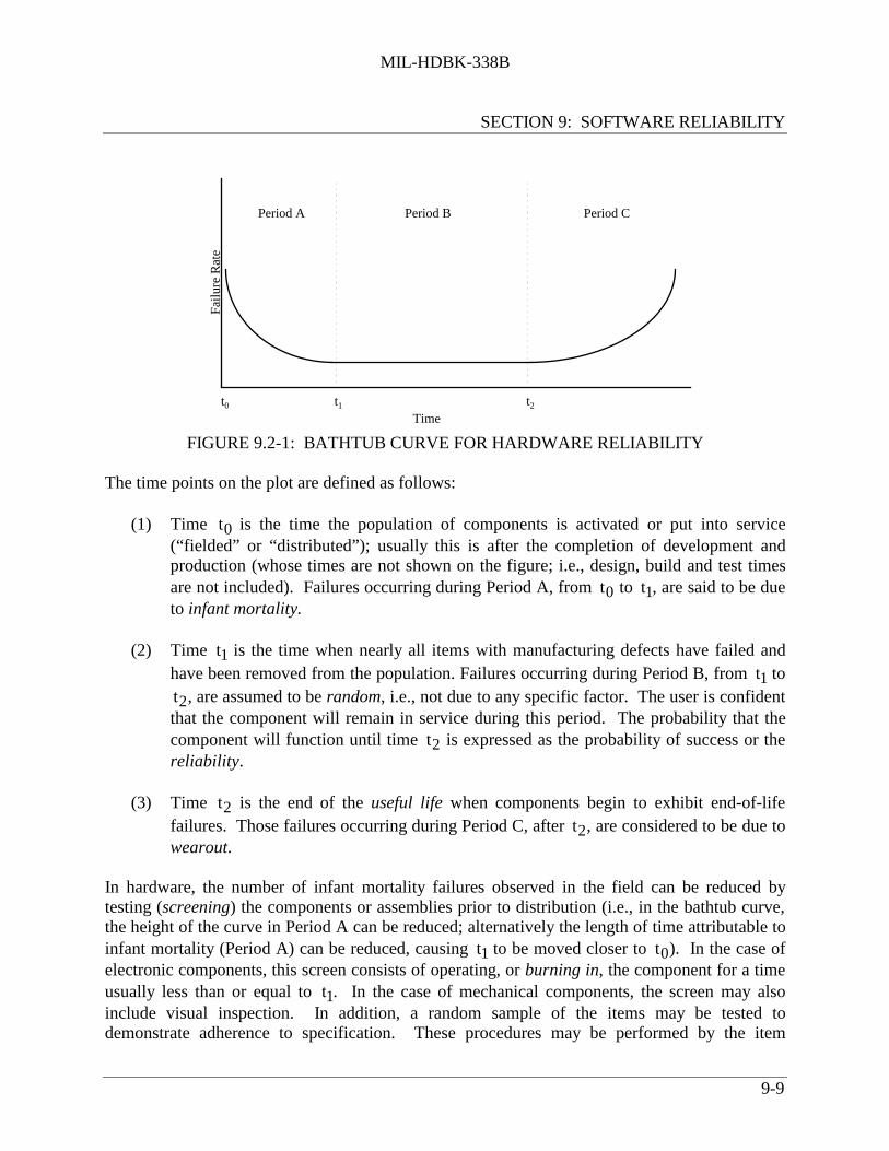
Life Cycle Considerations. Hardware reliability often assumes that the hazard rate (i.e., failurerate per unit time, often shortened to the failure rate) follows the “bathtub” curve, illustrated inFigure 9.2-1. Failures occur throughout the item’s life cycle; the hazard rate initially isdecreasing, then is uniform, and finally is increasing.



MIL-HDBK-338B


9-9

Fai

lure

Rat

ePeriod A

Time

Period CPeriod B

t1 t2t0

FIGURE 9.2-1: BATHTUB CURVE FOR HARDWARE RELIABILITY

The time points on the plot are defined as follows:

(1) Time t0 is the time the population of components is activated or put into service(“fielded” or “distributed”); usually this is after the completion of development andproduction (whose times are not shown on the figure; i.e., design, build and test timesare not included). Failures occurring during Period A, from t0 to t1, are said to be dueto infant mortality.

(2) Time t1 is the time when nearly all items with manufacturing defects have failed andhave been removed from the population. Failures occurring during Period B, from t1 to

t2, are assumed to be random, i.e., not due to any specific factor. The user is confidentthat the component will remain in service during this period. The probability that thecomponent will function until time t2 is expressed as the probability of success or thereliability.

(3) Time t2 is the end of the useful life when components begin to exhibit end-of-lifefailures. Those failures occurring during Period C, after t2, are considered to be due towearout.

In hardware, the number of infant mortality failures observed in the field can be reduced bytesting (screening) the components or assemblies prior to distribution (i.e., in the bathtub curve,the height of the curve in Period A can be reduced; alternatively the length of time attributable toinfant mortality (Period A) can be reduced, causing t1 to be moved closer to t0). In the case ofelectronic components, this screen consists of operating, or burning in, the component for a timeusually less than or equal to t1. In the case of mechanical components, the screen may alsoinclude visual inspection. In addition, a random sample of the items may be tested todemonstrate adherence to specification. These procedures may be performed by the item

MIL-HDBK-338B


9-10

manufacturer prior to distribution to ensure that shipped components have few or no latentfailures. Otherwise, the purchasing organization takes the responsibility for these activities.

When modeling the failure characteristics of a hardware item, the factors which contribute to therandom failures must be investigated. The majority are due to two main sources:

(1) Operating stress is the level of stress applied to the item. The operating stress ratio isthe level of stress applied relative to its rated specification. For example, a resistorrated to dissipate 0.5 watts when actually dissipating 0.4 watts is stressed at 80% ofrated. Operating stresses are well defined and measurable.

(2) Environmental stresses are considered to be those due to the specific environment(temperature, humidity, vibration, etc.) that physically affect the operation of the itembeing observed. For example, an integrated circuit having a rated temperature range of0° to 70°C that is being operated at 50°C is within operational environmentspecification. Environmental stresses also can be well defined and measurable.

When transient stresses occur in hardware, either in the operating stresses or the environmentalstresses, failures may be induced which are observed to be random failures. For this reason,when observing failures and formulating modeling parameters, care must be taken to ensureaccurate monitoring of all of the known stresses.

The same “bathtub” curve for hardware reliability strictly does not apply to software sincesoftware does not typically wearout. However, if the hardware life cycle is likened to thesoftware development through deployment cycle, the curve can be analogous for times up to t2.For software, the time points are defined as follows:

(1) Time t0 is the time when testing begins. Period A, from t0 to t1, is considered to bethe debug phase. Coding errors (more specifically, errors found and corrected) oroperation not in compliance with the requirements specification are identified andresolved. This is one key difference between hardware and software reliability. The“clock” is different. Development/test time is NOT included in the hardware reliabilitycalculation but is included for software.

(2) Time t1 is the initial deployment (distribution) time. Failures occurring during PeriodB, from t1 to t2, are found either by users or through post deployment testing. Forthese errors, work-arounds or subsequent releases typically are issued (but notnecessarily in direct correspondence to each error reported).

(3) Time t2 is the time when the software reaches the end of its useful life. Most errorsreported during Period C, after t2, reflect the inability of the software to meet thechanging needs of the customer. In this frame of reference, although the software isstill functioning to its original specification and is not considered to have failed, that



MIL-HDBK-338B


9-11

specification is no longer adequate to meet current needs. The software has reached theend of its useful life, much like the wearout of a hardware item. Failures reportedduring Period C may be the basis for generating the requirements for a new system.

Usually hardware upgrades occur during Period A, when initial failures often identify requiredchanges. Software upgrades, on the other hand, occur in both Periods A and B. Thus, the PeriodB line is not really “flat” for software but contains many mini-cycles of Periods A and B: anupgrade occurs, most of the errors introduced during the upgrade are detected and removed,another upgrade occurs, etc. Hence, Figure 9.2-2 might be a better representation of the softwarelife cycle. Although the failure rate drops after each upgrade in Period B, it may not reach theinitial level achieved at initial deployment, t1. Since each upgrade represents a minidevelopment cycle, modifications may introduce new defects in other parts of the softwareunrelated to the modification itself. Often an upgrade focuses on new requirements; its testingmay not typically encompass the entire system. Additionally, the implementation of newrequirements may inversely impact (or be in conflict with) the original design. The moreupgrades that occur, the greater the likelihood that the overall system design will becompromised, increasing the potential for increased failure rate, and hence lower reliability. Thisscenario is now occurring in many legacy systems which have recently entered Period C,triggering current reengineering efforts.

Failu

re R

ate

Period A

Time

Period CPeriod B

t1 t2t0

Upgrade

Upgrade

Upgrade

FIGURE 9.2-2: REVISED BATHTUB CURVE FOR SOFTWARE RELIABILITY

In software, the screening concept is not applicable since all copies of the software are identical.Additionally, typically neither operating stresses nor operational environment stresses affectsoftware reliability. The software program steps through the code without regard for thesefactors. Other quality characteristics, such as speed of execution, may be effected, however. Theend user might consider a “slow” program as not meeting requirements.

Table 9.2-2 summarizes the fundamental differences between hardware and software life cycles.

MIL-HDBK-338B


9-12

TABLE 9.2-2: SUMMARY: LIFE CYCLE DIFFERENCES

Life Cycle Pre t0

Period A(t0 to t1)

Period B(t1 to t2)

Period C(Post t2)

HARDWARE ConceptDefinitionDevelopmentBuildTest

DeploymentInfant MortalityUpgrade

Useful Life Wearout

SOFTWARE ConceptDefinitionDevelopmentBuild

TestDebug/Upgrade

DeploymentUseful LifeDebug/Upgrade

Obsolescence

9.3 Software Design

Once the requirements have been detailed and accepted, the design will be established through aprocess of allocating and arranging the functions of the system so that the aggregate meets allcustomer needs. Since several different designs may meet the requirements, alternatives must beassessed based on technical risks, costs, schedule, and other considerations. A design developedbefore there is a clear and concise analysis of the system’s objectives can result in a product thatdoes not satisfy the requirements of its customers and users. In addition, an inferior design canmake it very difficult for those who must later code, test, or maintain the software. During thecourse of a software development effort, analysts may offer and explore many possible designalternatives before choosing the best design.

Frequently, the design of a software system is developed as a gradual progression from a high-level or logical system design to a very specific modular or physical design. Many developmentteams, however, choose to distinguish separate design stages with specific deliverables andreviews upon completion of each stage. Two common review stages are the preliminary designand the detailed design.

9.3.1 Preliminary Design

Preliminary or high-level design is the phase of a software project in which the major softwaresystem alternatives, functions, and requirements are analyzed. From the alternatives, thesoftware system architecture is chosen and all primary functions of the system are allocated to thecomputer hardware, to the software, or to the portions of the system that will continue to beaccomplished manually.

During the preliminary design of a system, the following should be considered:

(1) Develop the architecture• system architecture -- an overall view of system components• hardware architecture -- the system’s hardware components and their interrelations• software architecture -- the system’s software components and their interrelations



MIL-HDBK-338B


9-13

(2) Investigate and analyze the physical alternatives for the system and choose solutions

(3) Define the external characteristics of the system

(4) Refine the internal structure of the system by decomposing the high-level softwarearchitecture

(5) Develop a logical view or model of the system’s data

9.3.1.1 Develop the Architecture

The architecture of a system describes its parts and the ways they interrelate. Like blueprints fora building, there may be various software architectural descriptions, each detailing a differentaspect. Each architecture document usually includes a graphic and narrative about the aspect it isdescribing.

The software architecture for a system describes the internal structure of the software system. Itbreaks high-level functions into subfunctions and processes and establishes relationships andinterconnections among them. It also identifies controlling modules, the scope of control,hierarchies, and the precedence of some processes over others. Areas of concern that are oftenhighlighted during the establishment of the software architecture include: system security, systemadministration, maintenance, and future extensions for the system.

Another aspect of the software architecture may be the allocation of resource budgets for CPUcycles, memory, I/O, and file size. This activity often leads to the identification of constraints onthe design solution such as the number of customer transactions that can be handled within agiven period, the amount of inter-machine communication that can occur, or the amount of datathat must be stored.

The first software architecture model for a system is usually presented at a very high level withonly primary system functions represented. An example of a high-level software architecture ispresented in Figure 9.3-1. As design progresses through detailed design, the architecture iscontinually refined.

9.3.1.2 Physical Solutions

Unless a software system has been given a pre-defined physical solution, an activity calledenvironmental selection occurs during the preliminary design of a system. This is the process ofinvestigating and analyzing various technological alternatives to the system and choosing asolution based upon the system’s requirements, the users’ needs, and the results of the feasibilitystudies. Aspects of a system that are generally selected at this time are: the hardware processingunit; computer storage devices; the operating system; user terminals, scanners, printers and otherinput and output devices; and the computer programming language.

MIL-HDBK-338B


9-14

In some cases, hardware and software items such as communications hardware and software,report writers, screen management systems, or database management systems are available “off-the-shelf.” In other cases, unique requirements of the system may dictate the development ofspecific hardware and software items, specially designed for the system. The additionalresources required to customize the system must be estimated and reviewed.

DatabaseA

DatabaseB

Process 2

Process 1

Process 4

Process 3

Process 5

Process B1

Process B3

Process B2

BULLETIN

BOARD

BULLETIN

BOARD

FIGURE 9.3-1: HIGH-LEVEL SOFTWARE ARCHITECTURE EXAMPLE

9.3.1.3 External Characteristics

Following the software system’s functional allocation and physical environment selection, thedetails of the external or observable characteristics of a system can be developed. Included herewould be terminal screen displays, report formats, error message formats, and interfaces to othersystems.

A human factors engineer may be part of the design team concerned with the observablecharacteristics of a software system. This person specializes in the analysis of the human-machine interface. When a system’s targeted users are novice computer users or when a systemrequires extensive manual data entry, human factors engineering can be a very important aspectof the design.



MIL-HDBK-338B


9-15

9.3.1.4 System Functional Decomposition

The activity of breaking a high-level system architecture into distinct functional modules orentities is called functional decomposition. When preparing to decompose a software system, thedesign team must decide what strategy they will use. Many decomposition strategies have beenwritten about and are advocated; most the variations of the widely used top-down or bottom-upapproaches. (Ref. [13]).

Top-down design is the process of moving from a global functional view of a system to a morespecific view. Stepwise refinement is one technique used in top-down design. With this method,design begins with the statement of a few specific functions that together solve the entireproblem. Successive steps for refining the problem are used, each adding more detail to thefunctions until the system has been completely decomposed.

A bottom-up design strategy for a software system is often used when system performance iscritical. In this method, the design team starts by identifying and optimizing the mostfundamental or primitive parts of the system, and then combining those portions into the moreglobal functions. (Ref. [14] and [15]).

9.3.2 Detailed Design

Detailed design or low-level design determines the specific steps required for each component orprocess of a software system. Responsibility for detailed design may belong to either the systemdesigners (as a continuation of preliminary design activities) or to the system programmers.

Information needed to begin detailed design includes: the software system requirements, thesystem models, the data models, and previously determined functional decompositions. Thespecific design details developed during the detailed design period are divided into threecategories: for the system as a whole (system specifics), for individual processes within thesystem (process specifics), and for the data within the system (data specifics). Examples of thetype of detailed design specifics that are developed for each of these categories are given below.

9.3.2.1 Design Examples

System specifics:

(1) Physical file system structure(2) Interconnection records or protocols between software and hardware components(3) Packaging of units as functions, modules or subroutines(4) Interconnections among software functions and processes(5) Control processing(6) Memory addressing and allocation(7) Structure of compilation units and load modules

MIL-HDBK-338B


9-16

Process specifics:

(1) Required algorithmic details(2) Procedural process logic(3) Function and subroutine calls(4) Error and exception handling logic

Data specifics:

(1) Global data handling and access(2) Physical database structure(3) Internal record layouts(4) Data translation tables(5) Data edit rules(6) Data storage needs

9.3.2.2 Detailed Design Tools

Various tools such as flowcharts, decision tables, and decision trees are common in detailedsoftware design. Frequently, a structured English notation for the logic flow of the system’scomponents is also used. Both formal and informal notations are often lumped under the termpseudocode. This is a tool generally used for the detailed design of individual softwarecomponents. The terminology used in pseudocode is a mix of English and a formalprogramming language. Pseudocode usually has constructs such as “IF ..., THEN ...,” or “DO ...UNTIL ...,” which can often be directly translated into the actual code for that component. Whenusing pseudocode, more attention is paid to the logic of the procedures than to the syntax of thenotation. When pseudocode is later translated into a programming language, the syntacticalrepresentation becomes critical.

9.3.2.3 Software Design and Coding Techniques

Specific design and code techniques are related to error confinement, error detection, errorrecovery and design diversity. A summary of the each technique is included in Table 9.3-1 andTable 9.3-2.



MIL-HDBK-338B


9-17

TABLE 9.3-1: SOFTWARE DESIGN TECHNIQUES

Design Techniques• Recovery designed for hardware failures• Recovery designed for I/O failures• Recovery designed for communication failures• Design for alternate routing of messages• Design for data integrity after an anomaly• Design for replication of critical data• Design for recovery from computational failures• Design to ensure that all required data is available• Design all error recovery to be consistent• Design calling unit to resolve error conditions• Design check on inputs for illegal combinations of data• Design reporting mechanism for detected errors• Design critical subscripts to be range tested before use• Design inputs and outputs within required accuracy

TABLE 9.3-2: SOFTWARE CODING TECHNIQUES

Coding Techniques• All data references documented• Allocate all system functions to a CSCI• Algorithms and paths described for all functions• Calling sequences between units are standardized• External I/O protocol formats standardized• Each unit has a unique name• Data and variable names are standardized• Use of global variables is standardized• All processes within a unit are complete and self

contained• All inputs and outputs to each unit are clearly defined• All arguments in a parameter list are used• Size of unit in SLOC is within standard• McCabe’s complexity of units is within standard• Data is passed through calling parameters• Control returned to calling unit when execution is

complete

• Temporary storage restricted to only one unit - notglobal

• Unit has single processing objective• Unit is independent of source of input or destination

of output• Unit is independent of prior processing• Unit has only one entrance and exit• Flow of control in a unit is from top to bottom• Loops have natural exits• Compounded booleans avoided• Unit is within standard on maximum depth of nesting• Unconditional branches avoided• Global data avoided• Unit outputs range tested• Unit inputs range tested• Unit paths tested

9.4 Software Design and Development Process Model

Software development can occur with no formal process or structure (called “ad hoc”development) or it can follow one of several approaches (i.e., methods or models). Ad hocdevelopment usually is the default used by relatively inexperienced developers or by those whoonly develop software as an aside or on rare occasions. As developers become moreexperienced, they tend to migrate from operating in an ad hoc fashion to using more formalstructured methodologies. These major software development process models have evolvedbased upon actual practice. The selection is based upon several basic concepts, as summarized in

MIL-HDBK-338B


9-18

Table 9.4-1 and described throughout this section.

However, it is important to realize that what is actually being practiced may not fully correspondto the theory of any one model. In reality, developers often customize a model by implementingone or a combination of several elements of the models described. What is important is tounderstand enough about what constitutes the organization’s software development process to beable to identify what characterizes the process used and to determine whether it is stable. Theprocess that is in place will determine not only what data are available but also when they areavailable and whether they are adequate for determining the software reliability and qualityperformance levels as defined by the customer’s contract requirements.

TABLE 9.4-1: SOFTWARE DEVELOPMENT PROCESS SELECTION

Approach When to UseWaterfall Model orClassic Development Model

When the detailed requirements are known, and are very stableWhen the type of application has been developed beforeWhen the type of software class (e.g., compilers or operating systems) has beendemonstrated to be appropriateWhen the project has a low risk in such areas as getting the wrong interface or notmeeting stringent performance requirementsWhen the project has a high risk in budget and schedule predictability and control

Prototyping Approach When the input, processing, or output requirements have not been identifiedTo test concept of design or operationTo test design alternatives and strategiesTo define the form of the man-machine interface

Spiral Model To identify areas of uncertainty that are sources of project riskTo resolve risk factorsTo combine the best features of the classic model and prototyping

Incremental Model When a nucleus of functionality forms the basis for the entire systemWhen it is important to stabilize staffing over the life of the project

Cleanroom Model When a project can be developed in incrementsWhen staff size is sufficient to perform independent testing (staff > 6)When the approach has management support



MIL-HDBK-338B


9-19

9.4.1 Ad Hoc Software Development

The reality in many organizations where software development is not the main focus is that thedevelopment process is ad hoc. This is a polite way of saying that a defined structured processdoes not exist. The development effort is subject to the habits and operating styles of theindividuals who comprise the project team. Responsibility for the project, and for interactionwith the customer, is often in the hands of a non-software engineer. The software is viewed ashaving a supporting role to the project as a whole. Communication regarding requirements isprimarily verbal and seldom documented. It is assumed that requirements are understood by allparties. Additionally, requirements change throughout the development effort. There is seldom afocus on design; design and code become merged into one task. Testing is the responsibility ofthe development team, and is often reduced to a random selection of functionality because thereis no time to do a thorough job. Documentation, including design documents, is often writtenafter the code is completed, and then reflects what was developed rather than serving as a guidefor development. The project schedule is often determined by who is available to work ratherthan who is best qualified, the amount of dollars available, and an arbitrary completion date thattypically is derived from something other than the functionality to be developed. The drivingforce is “having something to show by a specified date.”

9.4.2 Waterfall Model

The Waterfall Model is presented in Figure 9.4-1. In its most simplistic interpretation it suggeststhat the process is strictly sequential, that there is a flow of ideas through the phases, with eachphase having a distinct beginning and end and each phase enhancing the development to result ina software product that is operational when the bottom of the waterfall is reached.

The original intention of this model was that the development process is stable if all reworkrequires going back only one step in the process in order to be rectified. For example, if analysisrevealed that initial requirements were incomplete then further requirements gathering would beimplemented. If a particular design could not be coded correctly in the given environment thenthe design would be revisited. Testing would uncover coding errors which would be fixed beforefinal delivery. The model suggests that the phases follow a time line, but this does not allow forrevisiting previous phases when a problem is discovered.

MIL-HDBK-338B


9-20

SystemFeasibility

Validation

Software Plans &Requirements

Validation

Product Design

Verification

Code

Unit Test

Integration

ProductVerification

Implementation

System Test

Operations andMaintenance

Revalidation

Verification

Detailed Design

FIGURE 9.4-1: WATERFALL MODEL (REF. [6])

9.4.3 Classic Development Model

The Waterfall Model was later augmented to include precise phase ends and continuingactivities, and has come to be known as the Classic Development Model; see Figure 9.4-2. Thismodel provides a systemic approach to software development consisting of consecutive phasesthat begin with system engineering (sometimes called system requirements definition) andprogress through requirements analysis, design, coding, testing, and maintenance. Each phase isdefined in Figure 9.4-2.



MIL-HDBK-338B


9-21

SystemEngineering

Analysis

Design

Code

Testing

Maintenance

SystemDesignReview Software

SpecificationReview Software

DesignReview Test

ReadinessReview

PHASE DESCRIPTION

SystemEngineering(sometimes calledRequirementsDefinition)

When software is part of a larger system, work begins by establishing requirements for all system elementsand then allocating some subset of these requirements to software. This is essential since software mustinterface with other elements such as hardware, people, and databases. Requirements are defined at thesystem level with a small amount of top-level design and analysis. It is during this phase that developersidentify previously developed subsystems that can be reused on the current system.

RequirementsAnalysis

The requirements definition process is now intensified and focused specifically on the software. Thedevelopment team performs functional or object-oriented analysis and resolves ambiguities, discrepancies,and to-be-determined (TBD) specifications. To understand the nature of the software to be built, thedevelopers must understand the information domains for the software, as well as the required functions,performance, and interfaces. Requirements for both the system and the software are documented andreviewed with the sponsor/user.

Design Software design is actually a multi-step process that focuses on four distinct attributes of the software: datastructure, software architecture, procedural detail, and interface characterization. The design processtranslates requirements into a representation of the software that can be assessed for quality before codingbegins. During this step, the developers perform structured, data driven, or object-oriented analysis. Likerequirements, the design is documented and becomes part of the software configuration.

Code The design is translated (coded) into a machine-readable form. If design has been performed in a detailedmanner, coding can be accomplished mechanistically. The developers also reuse existing code (modules orobjects), with or without modification, and integrate it into the evolving system.

Test Once new code has been generated or reused code has been modified, software testing begins. The unit testprocess focuses on the logical internals of the software, ensuring that all statements have been tested. Theintegration and system testing process focuses on the functional externals, testing to uncover errors and toensure that the defined input will produce actual results that agree with required results. During acceptancetesting, a test team that is independent of the software development team examines the completed system todetermine if the original requirements are met. After testing the software is delivered to the customer.

Maintenance Software may undergo change (one possible exception is embedded software) after it is delivered for severalreasons (i.e., errors have been encountered, it must be adapted to accommodate changes in its externalenvironment (e.g., new operating system), and/or customer requires functional or performance enhancements).Software maintenance reapplies each of the preceding phases, but does so in the context of the existingsoftware.

FIGURE 9.4-2: THE CLASSIC DEVELOPMENT MODEL (REF. [7])

MIL-HDBK-338B


9-22

The Classic Development Model includes the notion of validation and verification at each of thephases. Validation is defined as testing and evaluating the integrated system to ensurecompliance with the functional performance and interface requirements. Verification is definedas determining whether or not the product of each phase of the software development processfulfills all the requirements resulting from the previous phase. The purpose of the validationassociated with the analysis and design model phases is to determine if the right product is beingbuilt. In revalidation activity that occurs after the software functionality has been defined, thepurpose is to determine if the right product is still being built. Verification activity, associatedwith product design is to determine if the product is being built right, including the rightcomponents and their inter-combinations. This Classic Model has a definite and important rolein software engineering history. It provides a template into which methods for analysis, design,coding, testing, and maintenance can be placed. It remains the most widely used proceduralmodel for software engineering.

The classic model does have weaknesses. Among the problems that are sometimes encounteredwhen the classic development process model is applied are:

(1) It emphasizes fully elaborated documents as completion criteria for early requirementsand design phases. This does not always work well for many classes of software,particularly interactive end-user applications. Also, in areas supported by fourth-generation languages (such as spreadsheet or small business applications), it isunnecessary to write elaborate specifications for one’s application before implementingit.

(2) Often the customer cannot state all requirements explicitly. The classic model requiresthis and has difficulty accommodating the natural uncertainty that exists at thebeginning of many projects.

(3) The customer must have patience. A working version of the program is not availableuntil late in the project schedule. Errors in requirements, if undetected until theworking program is reviewed, can be costly.

9.4.4 Prototyping Approach

Prototyping is a process that enables the developer to create a model of the software to be built.The steps for prototyping are identified and illustrated in Figure 9.4-3. The model can take oneof three forms:

(1) A model that depicts the human-machine interaction in a form that enables the user tounderstand how such interaction will occur

(2) A working prototype that implements some subset of the functions required of thedesired software



MIL-HDBK-338B


9-23

(3) An existing program that performs part or all of the functions desired, but has otherfeatures that will be improved upon in the new development effort

RequirementsGathering

and Refinement

QuickDesign

BuildingPrototype

CustomerEvaluation of

Prototype

RefiningPrototype

EngineerProduct

Start

Stop

Step DescriptionRequirementsGathering andRefinement

The developer and customer meet and define the overall objectives forthe software, identify whatever requirements are known, and outlineareas where further definition is mandatory.

Quick Design The quick design focuses on a representation of those aspects of thesoftware that will be visible to the user (e.g., user interface and outputformats).

PrototypeConstruction

A prototype is constructed to contain enough capability for it to be usedto establish or refine requirements, or to validate critical designconcepts. If a working prototype is built, the developer should attemptto make use of existing software or apply tools (e.g., report generators,window manager) that enable working programs to be generatedquickly.

CustomerEvaluation

The prototype is evaluated by the customer and is used to refinerequirements or validate concepts.

PrototypeRefinement

The process of iteration occurs as the prototype is “tuned” to satisfy theneeds of the customer, while at the same time enabling the developer tobetter understand what needs to be done.

FIGURE 9.4-3: STEPS IN THE PROTOTYPING APPROACH

Using an iterative rapid prototyping approach, the concept of the software system graduallyunfolds; each iteration continues to explore the functionality that is desired. This process iscomparable to performing “what if” analyses. The developer uses the prototype to generatesuggestions from users, including ideas for innovations and plans for revision of the prototypeitself, or the process it supports.

MIL-HDBK-338B


9-24

Rapid prototyping can significantly improve the quality and reliability of software if themethodology is properly used. However there are severe adverse impacts to quality andreliability when the developer or the customer perceives the prototype to be the completedproject. Adversaries of prototyping claim that prototyping should not replace the traditionaldevelopment cycle for these reasons:

(1) If a system is needed badly the prototype may be accepted in its unfinished state andpressed into service without necessary refinement. Eventually, as deficiencies arerealized, a backlash is likely to develop, requiring maintenance efforts which areextremely costly compared to the cost of doing it right the first time.

(2) It tends to shape the approach to a capability before it is thoroughly understood.

(3) The real costs of supporting prototypes after delivery are not well documented.Therefore there is little evidence to support statements claiming that the cost ofsoftware is less for systems developed under rapid prototyping methods.

(4) Prototyping can be difficult to manage as a project within a larger project.

The key to successful prototyping is to define the rules of the game at the beginning; that is, thecustomer and developer must both agree that the prototype is built to serve as a mechanism fordefining requirements or validating critical design concepts. It is then discarded (at least in part)and the actual software is engineered with an eye toward quality and maintainability.

9.4.5 Spiral Model

The Spiral Model for software development is presented in Figure 9.4-4. This model has beendeveloped to encompass the best features of both the Classic Model and prototyping, while at thesame time adding the element of risk analysis that is missing in both these process models. In thesimplest sense it represents the normalization of a “trial and error” methodology. It is used toexplore the possibilities in situations where a need exists but the exact requirements are not yetknown.



MIL-HDBK-338B


9-25

Risk Analysis (RA)

Risk Analysis (RA)

Risk Analysis (RA)

OperationalPrototype

DetailedDesign

Code

RequirementsValidation

SoftwareProductDesign

SoftwareRqts

Concept ofOperation

RA

Evaluate Alternatives:Identify, Resolve Risks

Process Through Steps

Develop, VerifyNext-Level Product

Requirements Plan,Life Cycle Plan

Integration andTest Plan

DevelopmentPlan

Simulations, Models, Benchmarks

CumulativeCost

Determine Objectives,Alternatives, Constraints

ReviewCommit-mentPartition

Develop,VerifyNext-LevelProcess Plans

Evaluate ProcessAlternatives: Identify,Resolve Process Risks

PlanNext Phases

DetermineProcessObjectives,Alternatives,Constraints

ImplementationIntegration

and Test

Prototype 1 Prototype 2 Prototype 3

AcceptanceTest

UnitTest

Design Validationand Verification

FIGURE 9.4-4: SPIRAL MODEL (REF. [7])

The model defines four major activities represented by the four quadrants (starting at upper leftand progressing clockwise) of the figure:

(1) Planning: Determination of objectives, alternatives and constraints

(2) Risk analysis: Analysis of alternatives and identification/resolution of risks

(3) Engineering: Development of the “next-level” product

(4) Customer evaluation: Assessment of the results of engineering

With each iteration around the spiral (beginning at the center and working outward),progressively more complete versions of the software are built. During the first cycle around thespiral, objectives, alternatives, and constraints are defined and risks are identified and analyzed.If risk analysis indicates that there is uncertainty in requirements, prototyping may be used in theengineering quadrant to assist both the developer and the customer. Simulations and othermodels may be used to further define the problem and refine requirements. The customerevaluates the engineering work and makes suggestions for modification. Based on customer

MIL-HDBK-338B


9-26

input, the next phase of planning and risk analysis occur. At each cycle around the spiral, theculmination of risk analysis results in a “go, no-go” decision. If risk is too great, the project canbe terminated. However, if the flow around the spiral path continues, each path moves thedeveloper outward toward a more complete model of the system, and, ultimately, to theoperational system itself. Every cycle around the spiral requires engineering that can beaccomplished using either the classic or prototyping approaches.

Like the other development process models, the spiral model is not a panacea. The following aresome of the reasons why it is not right for all developments:

(1) It may be difficult to convince the sponsor that the evolutionary approach iscontrollable.

(2) It demands risk assessment expertise, and relies on this expertise for success.

(3) If major risk areas are not uncovered during risk analysis, problems will undoubtedlyoccur.

(4) The model itself is relatively new and has not been used as widely as the Classic orprototyping approaches. It will take a number of years before its effectiveness andefficiency can be determined with certainty.

9.4.6 Incremental Development Model

The Incremental Development Model can be followed using a sequential approach or an iterativeapproach. In a sequential approach, once a step has been completed, a developer never returns tothat step or to any step previous to that step. In an iterative approach, if there is sufficient reasonto do so, the developer may return to a previously completed step, introduce a change, and thenpropagate the effects of that change forward in the development. Projects actually can rarelyfollow the sequential forward flow. Iteration is generally necessary.

The Incremental Development Model is based on developing the software in increments offunctional capability with a series of overlapping developments and a series of staggereddeliveries. As indicated in Figure 9.4-5, each increment is developed under the phased approachdescribed for the Classic Development Model. Each increment undergoes structural, or top-leveldesign, detailed design, code and unit test, integration and test, and delivery. The nucleus of thesoftware, the “cornerstone” functionality that is the foundation for use, must be addressed in thestructural design of the first increment. Additional capability is then added with successiveincrements. Note that all software efforts do not lend themselves to incremental developmentbecause it is often not possible to distinguish a nucleus of functional capability.



MIL-HDBK-338B


9-27

Increment 1

Increment 2

Increment 3

Increment 4

Delivery

Delivery

Delivery

Delivery

CalendarTime

Specification StructuralDesign(S.D.)

DetailedDesign(D.D.)

Code andUnit Test(CAUT)

Integrationand Test(I&T)

S.D. D.D. CAUT I&T

S.D. D.D. CAUT I&T

S.D. D.D. CAUT I&T

FIGURE 9.4-5: INCREMENTAL DEVELOPMENT MODEL (REF. [7])

Incremental development has been used successfully on many large projects. It is frequentlyused when the technical risks make it difficult to predict time scales for development, or whenthere is uncertainty about some aspects of the project. This approach also tends to level out orflatten the project’s labor distribution curve. The design, program, and test teams can remain atrelatively constant strength dealing with each increment in turn. Additionally, increments areeasier to test and the cost of refinements is less expensive than with the single-shot ClassicDevelopment Model.

Incremental development is a useful approach when some functions within the software systemhave more stringent reliability requirements than others. Design efforts for a given increment canfocus on attaining the desired reliability. Another feature of incremental development is thatwhile the timeframe from project start to end may be identical to that of a project developed withthe classic model, this model places operational software in the customer’s hands long beforeproject end.

MIL-HDBK-338B


9-28

9.4.7 Cleanroom Model

Cleanroom Software Engineering (Ref. [8] and [9]) (CSE) or just “Cleanroom” is a metaphorthat comes from the integrated circuit manufacturing process where the environment must be freefrom all contaminants. If one were to rank all software development methodologies according tothe amount of structure inherent in the methodology, the ad hoc development would be the lowerbound (lack of structure) and cleanroom methodology would be the upper bound (verystructured). Figure 9.4-6 illustrates the essential steps of the cleanroom development process.

The uniqueness of this approach is that it has embedded principles of total quality such as the useof teams, use of statistical process control techniques, and the commitment to “Do the rightthings right the first time” into the development process. The approach focuses on the aspects ofthe development that have the greatest impact on quality. Software reliability is specificallydefined and measured as part of the certification process. Cleanroom Certification Test Teamsprovide scientific certification of software reliability -- they do not test it in.

Cleanroom methodology is premised on the notion that the best way to produce softwareapproaching zero defects is to focus on defect prevention by clarifying requirements, developingprecise functional and usage specifications, and then using them as the guide for planning anddesign, and for test development. It further presumes that correctness verification of the designwill detect and eliminate most remaining significant defects before the software is actually built.The design effort entails writing pseudo code which is then subjected to correctness verification.The resulting pseudo code is so thorough and precise that it can be easily translated into thespecified language. The actual coding is considered to be trivial relative to the development ofpseudo code because the complex logic is addressed during pseudo code development.

In this methodology, the focus of testing reflects usage, not the structure of the software. Usageis inherent in the execution behavior of the software. Statistical Usage Testing is a process oftesting software the way users intend to use it. The entire focus is on external system behavior,not on the internals of design and implementation. Test cases are randomly generated based onprobability distributions that model anticipated software use in all possible circumstancesincluding unusual and stressed situations. By definition, testing is designed to detect the moreserious and/or high frequency defects first. Thus this testing method is more effective atimproving software reliability in less time than traditional testing techniques. Data recordedincludes execution time up to the point of each failure in appropriate units (measured in CentralProcessing Unit (CPU) time, clock time, or number of transactions, etc.). After execution of thetest runs, the results are assessed and quality and performance measures computed.



MIL-HDBK-338B


9-29

Quality-Certification

Model

Customer Requirements

Specification

Function Usage

IncrementalDevelopment

Planning

Functional Specification Usage Specification

Interfail Times

Formal Design

Correctness Verification

StatisticalTest-CaseGeneration

Statistical Testing

Source Code Test Cases

Mean Time To Failure(MTTF) Estimates

Metric

FIGURE 9.4-6: THE CLEANROOM DEVELOPMENT PROCESS (REF. [10])

Advocates for this methodology claim good results, namely that it is possible to produce softwarethat approaches zero defects and deliver it on time and within budget. There is no way ofknowing if a software system has zero defects, but as failure-free executions occur during testing,given the completeness of test coverage, one can conclude that there is a high probability that thesoftware is at or near zero defects and will not fail during actual usage. The cleanroom approachhas been adopted by more than 30 software development organizations as noted in the “SoftwareTechnology Support Center Guide (1995).” The cleanroom methodology has been applied tonew systems, maintenance and evolution of existing systems, and re-engineering of problemsystems. As of the end of 1993, cleanroom methodology used to develop a variety of projectstotaling more than one million lines of code has shown extraordinary quality compared to

MIL-HDBK-338B


9-30

traditional results. A summary of cleanroom performance measures is given in Table 9.4-2. Itshould be noted, however, that these results are achieved with cleanroom teams composed ofadequately trained journeyman programmers.

TABLE 9.4-2: CLEANROOM PERFORMANCE MEASURES (REF. [11])

Software DevelopmentPractices

Defects DuringDevelopment(defects per

KLOC*)

OperationalFailures

(failures perKLOC)

ResultantProductivity(LOC*/Staff

Month)Traditional Software-as-art

50 - 60 15 - 18 Unknown

Software Engineering 20 - 40 2 - 4 75 - 475Cleanroom Engineering 0 - 5 < 1 > 750

* KLOC - Thousand Lines of Code * LOC - Lines of Code

Adversaries claim that it is an unrealistic methodology for the following reasons:

(1) The required statistical knowledge is beyond the realm of most software engineers.

(2) The testing strategies are too complicated to expect the average developer to use.

(3) It is too complicated for use on small projects.

(4) The paradigm shift required is so radical that software people will never accept it.

Software Reliability Prediction and Estimation Models

Software reliability models have been in existence since the early 1970’s; over 200 have beendeveloped. Certainly some of the more recent ones build upon the theory and principles of theolder ones. Some of the older models have been discredited based upon more recent informationabout the assumptions and newer ones have replaced them. This review of software reliability isnot meant to be an exhaustive review of every model ever developed but, rather, a discussion ofsome of the major models in use today, highlighting issues important to the reliability engineer.

Prediction vs. Estimation Models

Software reliability modeling is generally used for one of two purposes: to make predictions andfor estimation. Software reliability prediction models use historical data for similar systemswhile estimation models use data collected during test. Prediction, therefore, is usually lessaccurate than estimation. The objective of software prediction is to predict the potentialreliability (fault rate) early in the development process. Insight into potential reliability allows



MIL-HDBK-338B


9-31

improvements in software management to be considered before coding and testing start. Theobjective of the estimation process is to determine the number of faults remaining in the softwarejust prior to testing so that the length of the test can be determined. Table 9.5-1 provides acomparison of prediction and estimation models.

TABLE 9.5-1: COMPARING PREDICTION AND ESTIMATION MODELS

Issues Prediction Models Estimation Models

Data Reference Uses historical data Uses data from the current softwaredevelopment effort

When Used InDevelopmentCycle

Usually made prior todevelopment or test phases; can beused as early as concept phase

Usually made later in life cycle (aftersome data have been collected); nottypically used in concept ordevelopment phases

Time Frame Predict reliability at some futuretime

Estimate reliability at either presentor some future time

9.5.1 Prediction Models

The most basic prediction model involves the use of an organization’s internal data, based onextensive experience and tracking, to develop predictions. Four other prediction models havebeen developed: Musa’s Execution Time Model, (Ref. [12]), Putnam’s Model, (Ref. [5]), andtwo models developed at Rome Laboratory and denoted by their technical report numbers: theTR-92-52 Model (Ref. [16]) and the TR-92-15 Model (Ref. [17]). Each prediction model, itscapabilities and description of outputs is summarized in Table 9.5-2.

9.5.1.1 In-house Historical Data Collection Model

A few organizations predict software reliability by collecting and using the database ofinformation accumulated on each of their own software projects. Metrics employed includeProduct, Project Management, and Fault indicators. Statistical regression analysis typically isused to develop a prediction equation for each of the important project characteristics.Management uses this information to predict the reliability of the proposed software product aswell as to plan resource allocation.

MIL-HDBK-338B


9-32

TABLE 9.5-2: SOFTWARE RELIABILITY PREDICTION TECHNIQUES

Prediction Model Capabilities Description of OutputsHistorical DataCollection Model

Can be most accurate, if there isorganization wide commitment.

Produces a prediction of the failurerate of delivered software based oncompany wide historical data.

Musa’s Model Predicts failure rate at start of systemtest that can be used later in reliabilitygrowth models.

Produces a prediction of the failurerate at the start of system test.

Putnam’s Model The profile of predicted faults overtime and not just the total number isneeded. Can be used with the otherprediction models.

Produces a prediction in the form ofa predicted fault profile over the lifeof the project.

TR-92-52 Model Allows for tradeoffs. Produces a prediction in terms offault density or estimated number ofinherent faults.

TR-92-15 Model Has default factors for estimatingnumber of faults

Estimates faults during eachdevelopment phase.

9.5.1.2 Musa’s Execution Time Model

Developed by John Musa (Ref. [12]) of Bell Laboratories in the mid 1970s, this was one of theearliest reliability prediction models. It predicts the initial failure rate (intensity) of a softwaresystem at the point when software system testing begins (i.e., when time, t = 0). The initialfailure intensity, λ 0 , (faults per unit time) is a function of the unknown, but estimated, totalnumber of failures expected in infinite time, N. The prediction equation is shown below; termsare explained in Table 9.5-3.

o0 x wpk x = λ

For example, a 100 line (SLOC) FORTRAN program with an average execution rate of 150 linesper second has a predicted failure rate, when system test begins, of λ0 = k x p x w0 = (4.2E-7) x(150/100/3) x (6/1000) = .0126E-7 = 1.26E-9 faults per second (or 1 fault per 7.9365E8 secondswhich is equivalent to 1 fault per 25.17 years).

It is important to note that this time measure is execution time, not calendar time. Sincehardware reliability models typically are in terms of calendar time, it is not feasible to use Musa’sprediction in developing an overall system reliability estimate unless one is willing to assumethat calendar time and execution time are the same (usually not a valid assumption).



MIL-HDBK-338B


9-33

TABLE 9.5-3: TERMS IN MUSA’S EXECUTION TIME MODEL

Symbol Represents Value

k Constant that accounts for the dynamicstructure of the program and the varyingmachines

k = 4.2E-7

p Estimate of the number of executions pertime unit

p = r/SLOC/ER

r Average instruction execution rate,determined from the manufacturer orbenchmarking

Constant

SLOC Source lines of code (not including reusedcode)

ER Expansion ratio, a constant dependent uponprogramming language

Assembler, 1.0; Macro Assembler, 1.5;C, 2.5; COBAL, FORTRAN, 3; Ada,4.5

w0 Estimate of the initial number of faults inthe program

Can be calculated using: w0 = N x Bor a default of 6 faults/1000 SLOC canbe assumed

N Total number of inherent faults Estimated based upon judgment or pastexperience

B Fault to failure conversion rate; proportionof faults that become failures. Proportionof faults not corrected before the product isdelivered.

Assume B = .95; i.e., 95% of the faultsundetected at delivery become failuresafter delivery

9.5.1.3 Putnam’s Model

Trachtenberg (formerly of General Electric) and Gaffney (of then IBM Federal Systems, nowLoral) examined defect histories, by phases of the development process, for many projects ofvarying size and application type. Based on their work, Putnam (Ref. [5]) assigned the generalnormalized Rayleigh distribution to describe the observed reliability, where k and a are constantsfit from the data and t is time, in months:

R(t) = k exp(-at2 )

The corresponding probability density function, f(t), the derivative of R(t) with respect to t, is ofthe general form:

f(t) = 2ak t exp(-at2 )

Putnam further developed an ordinal (i.e., not equally spaced in real time) scale to represent the

MIL-HDBK-338B


9-34

development process milestones; see Table 9.5-4. Of special interest is Milestone 7, denoted by

td, corresponding to the end of the development phases and the beginning of full operationalcapability; this point was defined as occurring at the 95th percentile (i.e., 95% of all defects havebeen detected at this point in the software development). Using td as the reference basis, he thendeveloped the expressions for the model constants, a and k, in terms N and td. The finalequation to predict the expected number of defects per month as a function of the schedule monthand the total number of inherent defects, N, is given by:

f(t) = (6N/td2

) t exp (-3t2/td2

)

TABLE 9.5-4: PUTNAM’S TIME AXIS MILESTONES

Milestone # Milestone0 Feasibility study1 Preliminary design review, function design complete2 Critical design review, detailed design complete3 First code complete4 Start of system integration test5 Start of user systems test6 Initial operational capability; installation7 Full operational capability; reliability about 95% in routine usage8 99% reliability achieved by stress testing9 99.9% reliability, assumed debugged

For example, suppose a FORTRAN program is being developed; the plan is that it will be fully

operational (Milestone 7) in 10 calendar months resulting in td2 to be 102 or 100. The defects

expected per month during development are calculated using the expression:

f(t) = .06 N t exp (-.03t2 )

Calculation results are shown in Figure 9.5-1, where t is the month number, f(t) is the expectedproportion of the total number of defects to be observed in month t, and F(t) represents thecumulative proportion. The Milestone number, based on the planned development schedule isalso shown for comparison; Milestone 7, corresponding to the 95th percentile, is, indeed, inMonth 10, Milestone 8, at the 99th percentile, is expected to occur in scheduled Month 13, andMilestone 9, at .999, is not expected to be reached by the end of scheduled Month 15.



MIL-HDBK-338B


9-35

t f(t) F(t) Mile #

1 0.058 0.058

2 0.106 0.165 1

3 0.137 0.302

4 0.149 0.451 2

5 0.142 0.592

6 0.122 0.715 3

7 0.097 0.811 4

8 0.070 0.881 5

9 0.048 0.929 6

10 0.030 0.959 7

11 0.017 0.976

12 0.010 0.986

13 0.005 0.991 8

14 0.002 0.993

15 0.001 0.994

PROPORTION OF TOTAL N EXPECTED PER MONTH

.00

.05

.10

.15

.20

1 2 3 4 5 6 7 8 9 10 11 12 13 14 15MONTH

PROPORTION

FIGURE 9.5-1: EXPECTED PROPORTION OF THE TOTAL NUMBER OF DEFECTS

One major benefit of this model is that the expected number of faults can be predicted for variouspoints in development process as compared to Musa’s model that provides the prediction whensystem testing begins (i.e., at Milestone 4) only.

Another corollary to this model is that the mean time to the next defect (MTTD) is given by1/f(t). This is only meaningful after Milestone 4 (since prior to that point the system would nothave been developed so defects could not be detected). As the development progresses, (i.e., tincreases), the MTTD increases since defects are being eliminated.

9.5.1.4 Rome Laboratory Prediction Model: RL-TR-92-52 (Ref. [16])

This is a method for predicting fault density at delivery time (i.e., at Putnam’s Milestone 6) andsubsequently using this fault density to predict the total number of inherent faults, N, and thefailure rate. It also provides a mechanism for allocating software reliability as a function of thesoftware characteristics as well as assessing trade-off options. The basic terminology of thismodel is presented in Table 9.5-5. The underlying assumption is that Source Lines of Code(SLOC) is a valid size metric.

MIL-HDBK-338B


9-36

TABLE 9.5-5: RL-TR-92-52 TERMINOLOGY

Terms DescriptionA Factor selected based on Application type; represents the baseline fault densityD Factor selected to reflect the Development environmentS Factor calculated from various “sub-factors” to reflect the Software characteristics

SLOC The number of executable Source Lines Of Code; lines that are blank or containcomments to enhance the readability of the code are excluded

FD Fault density; for the purposes of this model it is defined as the ratio of faults tolines of code (faults/SLOC)

N Estimate of total number of inherent faults in the system; prediction is derived fromthe fault density and the system size

C Factor representing a Conversion ratio associated with each application type; valuesare determined by dividing the average operational failure rate by the average faultdensity in the baseline sample set.

It is recognized as one of a few publicly available prediction models based upon extensivehistorical information. Predictions are based on data collected on various types of softwaresystems developed for the Air Force; see Table 9.5-6.

TABLE 9.5-6: AMOUNT OF HISTORICAL DATA INCLUDED

Application Type # of Systems Total SLOCAirborne 7 540,617Strategic 21 1,793,831Tactical 5 88,252Process Control 2 140,090Production Center 12 2,575,427Developmental 6 193,435TOTAL 53 5,331,652

The basic equations are:

Fault Density = FD = A x D x S (faults/line)Estimated Number of Inherent Faults = N = FD x SLOCFailure Rate = FD x C (faults/time)

The model consists of factors that are used to predict the fault density of the software application.These factors are illustrated in Table 9.5-7.



MIL-HDBK-338B


9-37

TABLE 9.5-7: SUMMARY OF THE RL-TR-92-52 MODEL

Factor Measure Range of Values Phase Used In* Trade-off RangeA - Application Difficulty in developing

various application types2 to 14(defects/KSLOC)

A-T None - Fixed

D - Developmentorganization

Development organization,methods, tools, techniques,documentation

.5 to 2.0 If known at A, D-T

The largest range

SA - Softwareanomaly management

Indication of fault tolerantdesign

.9 to 1.1 Normally, C-T Small

ST - Softwaretraceability

Traceability of design andcode to requirements

.9 to 1.0 Normally, C-T Large

SQ - Software quality Adherence to codingstandards

1.0 to 1.1 Normally, C-T Small

SL - Softwarelanguage

Normalizes fault density bylanguage type

Not applicable C-T N/A

SX - Softwarecomplexity

Unit complexity .8 to 1.5 C-T Large

SM - Softwaremodularity

Unit size .9 to 2.0 C-T Large

SR - Softwarestandards review

Compliance with design rules .75 to 1.5 C-T Large

Key A - Concept or Analysis Phase

D - Detailed and Top Level DesignC - CodingT - Testing

The following are benefits of using this model:

(1) It can be used as soon as the concept of the software is known

(2) During the concept phase, it allows “what-if” analysis to be performed to determine theimpact of the development environment on fault density

(3) During the design phase, it allows “what-if” analysis to be performed to determine theimpact of software characteristics on fault density

(4) It allows for system software reliability allocation because it can be applied uniquely toeach application type comprising a software system

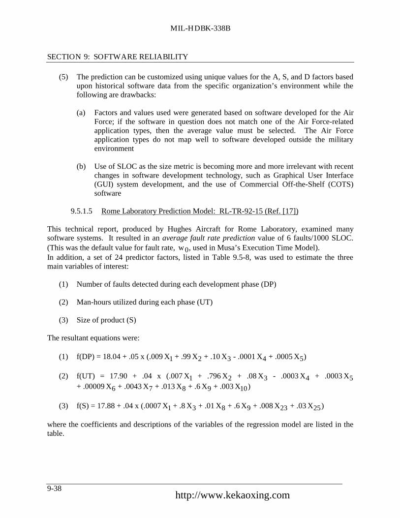
MIL-HDBK-338B


9-38

(5) The prediction can be customized using unique values for the A, S, and D factors basedupon historical software data from the specific organization’s environment while thefollowing are drawbacks:

(a) Factors and values used were generated based on software developed for the AirForce; if the software in question does not match one of the Air Force-relatedapplication types, then the average value must be selected. The Air Forceapplication types do not map well to software developed outside the militaryenvironment

(b) Use of SLOC as the size metric is becoming more and more irrelevant with recentchanges in software development technology, such as Graphical User Interface(GUI) system development, and the use of Commercial Off-the-Shelf (COTS)software

9.5.1.5 Rome Laboratory Prediction Model: RL-TR-92-15 (Ref. [17])

This technical report, produced by Hughes Aircraft for Rome Laboratory, examined manysoftware systems. It resulted in an average fault rate prediction value of 6 faults/1000 SLOC.(This was the default value for fault rate, w0, used in Musa’s Execution Time Model).In addition, a set of 24 predictor factors, listed in Table 9.5-8, was used to estimate the threemain variables of interest:

(1) Number of faults detected during each development phase (DP)

(2) Man-hours utilized during each phase (UT)

(3) Size of product (S)

The resultant equations were:

(1) f(DP) = 18.04 + .05 x (.009 X1 + .99 X2 + .10 X3 - .0001 X4 + .0005 X5)

(2) f(UT) = 17.90 + .04 x (.007 X1 + .796 X2 + .08 X3 - .0003 X4 + .0003 X5+ .00009 X6 + .0043 X7 + .013 X8 + .6 X9 + .003 X10)

(3) f(S) = 17.88 + .04 x (.0007 X1 + .8 X3 + .01 X8 + .6 X9 + .008 X23 + .03 X25)

where the coefficients and descriptions of the variables of the regression model are listed in thetable.



MIL-HDBK-338B


9-39

TABLE 9.5-8: REGRESSION EQUATION COEFFICIENTS

CoefficientsX Description of Variable EQ 1 EQ 2 EQ 31 Number of faults in software requirements specification .009 .007 .0072 Requirements statement in specification .99 .796 NA3 Pages in specification .10 .08 .804 Man-months spent in requirements analysis .0001 -.0003 NA5 Requirements change after baseline .0005 .0003 NA6 Number of faults in preliminary design document NA .00009 NA7 Number of CSCS NA .0043 NA8 Number of units in design NA .013 .019 Pages in design document NA .6 .6

10 Man-months spent in preliminary design NA .003 NA11 Number of failures in design document NA NA NA12 Man-months spent in detailed design NA NA NA13 Design faults identified after baseline NA NA NA14 Design faults identified after internal review NA NA NA15 Number of executable SLOC NA NA NA16 Faults found in code reviews NA NA NA17 Average years of programmer experience NA NA NA18 Number of units under review NA NA NA19 Average number of SLOC per unit NA NA NA20 Average number branches in unit NA NA NA21 Percentage branches covered NA NA NA22 Nesting depth coverage NA NA NA23 Number of times an unit is unit tested NA NA .00824 Man-months for coding and unit test NA NA NA25 Equals (X13 + X14 + X16) NA NA .03

The results indicate that thirteen of the 24 hypothesized factors had no effect on the threevariables of interest. Further, the most important estimators involved the software requirementsspecification, including the number of requirement statements, number of faults in thesestatements, and the total number of pages in the specification.

The benefits of this model are:

(1) It can be used prior to system testing to estimate reliability

(2) It includes cost and product parameters as well as fault and time

The disadvantages of this model are:

(1) It was based on data collected by one organization in one industry/application type

(2) It does not disclose the unit of measure for specification size

MIL-HDBK-338B


9-40

9.5.2 Estimation Models

The fault count and fault rate models are the most common type of estimation techniques. Eachmakes assumption about how faults arrive (detected) and how they are corrected. The fault countmodels include: Exponential, Weibull and Bayesian techniques. Also, included in theestimation model scenario are the test coverage and fault tagging methods.

9.5.2.1 Exponential Distribution Models

In general, exponential models assume that the software is in an operational state and that allfaults are independent of each other. The time to failure, t, of an individual fault follows theexponential distribution:

t)exp(- = f(t) λλ

with the general form for the reliability given by:

R(t) = exp(-λt)

and the mean time to the next failure (MTTF) expressed as:

MTTF = 1/λ

The notations used in the general case for the exponential distribution model are shown in Table9.5-9 and illustrated in Figure 9.5-2.



MIL-HDBK-338B


9-41

TABLE 9.5-9: NOTATIONS FOR THE EXPONENTIAL DISTRIBUTION MODEL

Notation ExplanationN Total number of defectsn Number of defects to datec Number of defects corrected to date

N-n Defects not yet manifestedN-c Defects yet to be correctednf Fault countλf Fault ratetf Future timenp Fault count at present timeλp Fault rate at present timetp Present time

N

nf

np

0

∆n

∆(n/t)

λf λP λ0

Numberof

Defects

Fault Rate

FIGURE 9.5-2: EXPONENTIAL MODEL BASIS

Advocates of the exponential model note its simplicity and its parallelism to the hardwarereliability framework. The major disadvantage is that it cannot be used early in the softwaredevelopment since the product must be operational before the model can be used. Hence, itcannot be used for early reliability assessment.

Table 9.5-10 summarizes the various exponential models including assumptions and comments.

MIL-HDBK-338B


9-42

TABLE 9.5-10: VARIOUS EXPONENTIAL MODELS*

Model MTTF Dn Dt Assumptions/CommentsGeneralExponential

1/[k(N - c)] k-1 λp / λf k-1 ln (λp / λf) Faults are equal in severity and probability ofdetectionFault rate directly related to number of faultsremaining to be corrected

Lloyd-Lipow 1/[k(N - n)] k-1 λp / λf k-1 ln (λp / λf) Fault rate directly related to number of faultsremaining to be detected

Musa’s Basic N/λ0 (λp - λf) N/λ0 ln (λp - λf) References an initial fault rate at time 0(beginning of system test)

Musa’sLogarithmic

f-1 ln (λp /λf) f-1 (1/λf -1/λp) Some faults are more likely to be foundbefore othersRate of fault detection decreasesexponentially

Shooman’s 1/[kSLOC -((N/SLOC) -(C/SLOC))]

k-1 λp / λf k-1 ln (λp / λf) Adjusts for changing product size; eachparameter is normalized for lines of code

Goel-Okumoto Faults can cause other faultsFaults may not be removed immediately

* where k is a constant of proportionality, N is the number of inherent faults, c is the number of corrected faults andn is the number of detected faults

General Exponential Model

In the general case, the model assumes that all faults are equal in severity and probability ofdetection and that each is immediately corrected upon detection. The fault rate, λ , is assumed tobe directly related to the number of faults remaining in the software. That is, λ is a function ofthe number of corrected faults, c:

c) - (Nk = λ

where k is a constant of proportionality. In actual application, k is typically estimated from theslope of the plot of the observed fault rate vs. number of faults corrected.

The projection of the number of faults needed to be detected to reach a final failure rate λ f isgiven by:

fp / (1/k) =n λλ∆

where k is the same proportionality constant used above.



MIL-HDBK-338B


9-43

The projection of the time necessary to reach a projected fault rate is given by:

[ ]fp /(1/k)ln =t λλ∆

The major disadvantage of this specific approach is that not only must the defects be detected butthey also must be corrected.

Lloyd-Lipow Model (Ref. [18] and [19])

The Lloyd-Lipow Model exponential model also assumes that all faults are equal in severity andprobability of detection. The difference from the previous model is that in this Lloyd-Lipowapproach, the fault rate, λ , is assumed to be directly related to the number of faults remaining tobe detected (not corrected) in the software. That is, λ is a function of the number of detectedfaults, n:

n) - (Nk = λ

The expressions for the mean-time-to-failure (MTTF), ∆n and ∆t are the same as in the generalexponential model.

This form of the exponential model does not require defect correction, just detection. However,the validity of the use of the exponential model in this situation has been questioned.

Musa’s Basic Model (Ref. [12])

Musa’s Basic Model is another form of the general exponential model. It utilizes the initial (i.e.,at the start of software testing) fault rate, λ0, where either λ0 is estimated from the data orcomputed ( λ0 = N/k) based on a guess for N and the estimate for k, the previously referencedslope value.

In this model, the fault rate after n faults have been detected is a fraction of the original fault rate:

λ n = λ0 (1 - n/v)

where:n is usually expressed as µ and v is usually expressed as υ

while the expression for the fault rate at time t is given by:

λ t = λ 0 exp [-(λ 0/υ)τ]

MIL-HDBK-338B


9-44

where:υ = N/B, where N is the number of inherent faults and B is the fault reduction ratio,

usually assumed to be 95% (i.e., 95% of the faults undetected at delivery becomefailures after delivery

τ = System test time


) - ( N/ =n fp0 λλλ∆

The projection of the time necessary to reach a projected failure rate is given by:

) - (ln N/ =t fp0 λλλ∆

The disadvantage is that this model is very sensitive to deviations from the assumptions. Inaddition, as noted with Musa’s previous work, the units are execution time, not calendar time.

Musa’s Logarithmic Model (Ref. [12])

Musa’s Logarithmic Model has different assumptions than the other exponential models:

(1) Some faults are likely to be found before others

(2) The rate of fault detection is not constant, but decreases exponentially

In this model, the fault rate after n faults have been detected is a function of the original faultrate:

exp(-ft) = 0n λλ

while the expression for the fault rate at time t is given by:

1) + t f /( = 00t λλλ

where:f = failure intensity decay parameter, the relative change of n/t over n.



MIL-HDBK-338B


9-45


)/(ln /f1 =n fp λλ∆

The projection of the time necessary to reach a projected failure rate is given by:

)1/ - (1/ 1/f =t pf λλ∆

The major benefit of this model is that it does not require an estimate for N. Since the value for fcan be estimated prior to actual data occurrence, the model can be used earlier in thedevelopment cycle to estimate reliability.

The disadvantage of this model, typical for most exponential models, is that the modelassumptions must be valid for the results to be valid. In particular, the assumption that the rate offault detection decreases exponentially has not been confirmed with many real data sets. Inaddition, as noted with Musa’s previous work, the units are execution time, not calendar time,making direct comparison with hardware reliability difficult.

Shooman’s Model (Ref. [20])

The Shooman’s Model is similar to the general exponential model except that each fault count isnormalized for the lines of code at that point in time. Earlier, λ = k (N - c); here, it is given by:

λ = k SLOC (N/SLOC - c/SLOC)

The equation of MTTF = 1/λ uses Shooman’s expression for λ . The equations for ∆n and ∆tare the same as the general exponential case.

The advantage of Shooman’s model is that it adjusts for the changing size of the softwareproduct. The disadvantages are that it must be used later in development after the LOC havebeen determined and that the general exponential assumptions may not apply.

Goel-Okumoto Model (Ref. [19])

This model is different from other exponential models because it assumes that faults can causeother faults and that they may not be removed immediately. An iterative solution is required.This model is expressed as:

exp(-bt) ab = tλ

MIL-HDBK-338B


9-46

where a and b are resolved iteratively from the following:

n/a = 1 - exp(-bt) and n/b = a t exp(-bt) + ∑ ti ,

where the summation is over i = 1,..., n,

Use N and k as starting points for solving for these two equations simultaneously.

The major benefit of this model is that it can be used earlier than other exponential models whileits major disadvantage is that it is very sensitive to deviations from the assumptions.

9.5.2.2 Weibull Distribution Model (Ref. [19])

The Weibull Model is one of the earliest models applied to software. It has the same form as thatused for hardware reliability. There are two parameters: a, the scale parameter (a > 0), and b, theshape parameter that reflects the increasing (b > 1), decreasing (b < 1) or constant (b = 1) failurerate.

The mean time to next failure is given by:

(1/a) (b/a) = MTTF Γ

where Γ (c) is the complete Gamma Function = 0

∞

∫ yc −1 e −ydy

The reliability at time t is given by:

R(t) = exp[-(t/b)a ]

The benefits of the Weibull model is its flexibility to take into account increasing and decreasingfailure rates. The disadvantage of this model is more work is required in estimating theparameters over the exponential model.

9.5.2.3 Bayesian Fault Rate Estimation Model

The Bayesian approach does not focus on the estimated inherent fault count, N, but ratherconcentrates on the fault/failure rate. The classical approach assumes that reliability and failurerate are a function of fault detection while the Bayesian approach, on the other hand, assumesthat a software program which has had fault-free operation is more likely to be reliable. TheBayesian approach also differs because it is possible to include an assessment of “priorknowledge” (therefore, it is sometimes called a “subjective” approach).



MIL-HDBK-338B


9-47

The Thompson and Chelson’s model (Ref. [19]) assumes that:

(1) Software is operational

(2) Software faults occur at some unknown rate λ that is assumed to follow a GammaDistribution with parameters Xi and fi + 1

(3) Faults are corrected in between test periods but not during test periods

(4) Total number of faults observed in a single testing period of length ti follows a Poissondistribution with parameter λti

The model assumes that there are i test periods, each with length, ti (not assumed equal); wherethe number of faults detected during that period is represented by fi . The subjective informationis inserted as occurring in period 0, i.e., t0 and f0 represent the prior information. If there is noprior information, these values are set to zero. On the other hand, if there is a great deal ofexperience, t0 might be very large, especially relative to the expected evaluation time; the valuefor the prior number of faults also depends on past experience and is independent from the priorof time.

Let Ti represent the cumulative total of the test period lengths over the entire range, i.e., fromperiod 0 to i and let Fi represent the cumulative total of the faults, fi , over the entire range, i.e.,from period 0 to i.

Then, the reliability at time t (in interval i) is expressed as a function of the values from the

previous (i - 1) interval as well as the current ith interval data:

R(t) = [Ti-1/(Ti-1 + t)]Fi-1

The failure rate estimate at time t (in interval i) is given by:

1-i1-i 1)/T + (F = (t)λ

The benefits of this model are related to its assumptions: N is not assumed fixed, reliability isnot assumed to be directly a function of N, and faults are not assumed to be correctedimmediately. The disadvantage is that Bayesian Models, in general, are not universally acceptedsince they allow for the inclusion of prior information reflecting the analyst’s degree of beliefabout the failure rate.

MIL-HDBK-338B


9-48

9.5.2.4 Test Coverage Reliability Metrics

Test coverage advocates have defined software reliability as a function of the amount of thesoftware product that has been successfully verified or tested. Three such metrics are discussedbelow. The first is a simple ratio based upon the rate of successful testing during the finalacceptance test. The second and third provide a metric based on ways of combining the resultsfrom both white-box and black-box testing.

Advocates of this approach to reliability explain that since the data are (or should be) collectedand tracked during testing, these measures are readily available and require no additionalverification effort. However, to the reliability engineer, these metrics are foreign to anythingused in the hardware environment to describe reliability. Further, none of these metrics can beconverted to failure rate or used to predict or estimate mean time between failures.

Test Success Reliability Metric

In this approach, (Ref. [19]) reliability is simply defined as the ratio of the number of test casesexecuted successfully during acceptance (black-box) testing, defined as s, to the total number oftest cases executed during acceptance testing, defined as r:

R = s/r

The validity of the result is dependent on the size of r as well as the ability for r to represent thetotal operational profile of the software. During the very late stages of testing, immediately priorto delivery, this model may be used for accepting or rejecting the software.

IEEE Test Coverage Reliability Metric

This method (Refs. [21] and [22]) assumes that reliability is dependent upon both the functionsthat are tested (black-box) and the product that is tested (white-box). It assumes that both typesof testing have to be completed for the test coverage to be complete. The reliability value isdefined as the product of two proportions, converted to a percent:

R = p(functions tested) * p(program tested) * 100%

where:p(functions tested) = Number of capabilities tested/total number of capabilities

p(program tested) = Total paths and inputs tested/total number of paths and inputs

Leone’s Test Coverage Reliability Metric

This approach (Ref. [23]) is similar to the IEEE Model except that it assumes that it is possibleto have either white or black box testing and still have some level of reliability. Two white-box



MIL-HDBK-338B


9-49

variables, a and b, and two black-box variables, c and d, are assessed. The reliability is theweighted sum of the four proportions:

R = ((a * w1) + (b * w2) + (c * w3) + (d * w4)) / (w1 + w2 + w3 + w4)

where:a = Number of independent paths tested/total number of pathsb = Number of inputs tested/total number of inputsc = Number of functions verified/total number of functionsd = Number of failure modes addressed/total number of failure modes

The values for w1, w2, w3, w4 represent weights. If all parameters are equally important, theseweights all are set to 1; however, if there are data to support that some parameters are moreimportant than others, then these more important parameters would receive higher weights.This model has two underlying assumptions. First, independent paths are identified usinginformation from testing procedures. Second, failure models (Ref. [24]) are identified usingFault Tree Analysis or Failure Modes, Effects, and Criticality Analysis.

9.5.3 Estimating Total Number of Faults Using Tagging

Tagging (Ref. [23]) is used to estimate the total number of faults in the software, N, based on thenumber observed during testing. It is based on seeding, a method of introducing faults into thesoftware and then determining how many of these faults are found during testing in order toestimate the total number of faults.

To illustrate, suppose the number of fish in a pond, N, is of interest. One way to develop anestimate is to capture and tag some number of the fish, T, and return them to the pond. As fishare caught, the number of tagged fish, t, is recorded as well as the number untagged, u. The totalnumber of untagged fish U, is estimated using the proportion: u/U = t/T. Then, the total numberof fish is estimated as the sum: N = U + T.

The steps used in the basic seeding approach for a software fault estimation are:

(1) A set of faults which represents the faults which would typically be found in operationalusage is identified.

(2) Faults are injected into software without the testers or developers being aware of them.The total number of injected faults is T.

(3) Test software and identify all faults found. Let t = the number of faults detected thatwere injected and let u = the number of faults detected which were not injected.

MIL-HDBK-338B


9-50

(4) The total number of faults which are not injected is estimated by U, where:

u/U = t/T

(5) The total number of faults, N, is estimated by:

N = U + T

(6) The injected faults are removed.

In general, this approach is not recommended based upon the issues identified below:

(1) How can faults which are typical of operational usage be identified and then injected ina completely random manner? (without bias)?

(2) Seeding assumes faults are due to coding mistakes. What about faults due torequirements, design and maintenance errors?

(3) During the course of a typical testing cycle, faults are typically corrected. Do theinjected faults get corrected during this process, or at the very end.

(4) Will seeded faults prevent real faults from being detected?(5) How can injected faults be kept a secret when the maintainer goes to fix them? How

can it be justified to spend resources fixing injected faults?(6) What is the action at the end of testing, go back to the original version with no injected

faults (and no corrected real faults) or remove (hopefully all) the injected faults?

An alternative Dual Test Group Approach is similar to basic seeding except that two groups areused. It assumes that:

(1) Two independent test groups are testing the same software at same time.(2) Groups do not share information on faults detected in testing.(3) Groups create their own test plans, but test the same functionality of the software.(4) Groups are equal in experience and capabilities.

This model predicts N, the total number of faults, based upon three numbers, n1, n2, and n12where n1 and n2 represent the number of faults found by Group 1 and Group 2, respectively,while n12 is the number of faults found by both groups.

The total number of faults, N, is estimated by:

N = R + n1 + n2 + n12

where:R is the estimated total number of remaining faults



MIL-HDBK-338B


9-51

This model assumes that as the number of faults found by both groups increases, the numberremaining decreases. As testing continues, it is assumed that n12 will increase. This means thatwhen there are few faults left in the software (i.e., as R approaches 0), both test groups will beginfinding the same faults. This may not be the case, however, since both test groups may beinefficient. The basic assumptions also may be unrealistic. It is not always possible oreconomical to have two completely independent test groups with equal experience level andcapabilities. It also may not be easy to keep the groups independent and equal in experience.

9.6 Software Reliability Allocation

Software reliability allocation involves the establishment of reliability goals for individualcomputer software configuration items (CSCI) based on top-level reliability requirements for allthe software. It is very important that this activity, allocations, be established early in theprogram so that criteria for evaluating the achieved reliability of each element can be established.Table 9.6-1 describes five allocation techniques. These techniques are based on the type ofexecution expected or the operational profile or the software complexity.

The allocation of a system requirement to software elements makes sense only at the softwaresystem or CSCI level. Once software CSCIs have been allocated reliability requirements, adifferent approach is needed to allocate the software CSCI requirements to lower levels. Thereliability model for software differs significantly from hardware due to its inherent operatingcharacteristics. For each mode in a software system’s (CSCI) operation, different softwaremodules (CSCs) will be executing. Each mode will have a unique time of operation associatedwith it. A model should be developed for the software portion of a system to illustrate themodules which will be operating during each system mode, and indicate the duration of eachsystem mode. An example of this type of model is shown in Table 9.6-2 for a missile system.

TABLE 9.6-1: SOFTWARE RELIABILITY ALLOCATION TECHNIQUES (REF. [2])

Technique Procedure Name Use DescriptionSequential Execution(see 9.6.1)

Equal apportionment applied tosequential software CSCIs

Use early in the SW development process whenthe software components are executedsequentially

Concurrent Execution(see 9.6.2)

Equal apportionment applied toconcurrent software CSCIs

Use early in the SW development process and thesoftware components are executed concurrently

Operational Profile(see Ref. [2])

Mission or Operational ProfileAllocation

Use when the operational profile of the CSCIs areknown

OperationalCriticality (see 9.6.3)

Allocation based on operationalcriticality factors

Use when the operational criticalitycharacteristics of the software is known

Complexity (see9.6.4)

Allocation based on complexityfactors

Use when the complexity factors of the softwarecomponents are known

The software reliability model will include the number of source lines of code (SLOC) expectedfor each module. These data, along with other information pertaining to software developmentresources (personnel, computing facilities, test facilities, etc.) are used to establish initial failureintensity predictions for the software modules.

MIL-HDBK-338B


9-52

To assist in the proper selection of an allocation technique, a flow diagram is provided in Figure9.6-1.

TABLE 9.6-2: SOFTWARE FUNCTIONS BY SYSTEM MODE - EXAMPLE

System Mode Modules SLOCStandby - 2 Hours Built-in Test (BIT)

1760 InterfaceFlight SequencingPrelaunch InitializationTOTAL

4000750

2000900

7650Prelaunch - 20 Minutes BIT

NavigationFlight SequencingPrelaunch InitializationNavigation Kalman FilterTOTAL

400010002000

90020009900

Post-Launch - 10 Minutes BITInterfaceNavigationInfrared Seeker ControlFlight SequencingTerminal ManeuverOther Post-LaunchNavigation Kalman FilterTOTAL

400070001000

50020001000

245002000

42000

Are the CSCIsexecuted

sequentially?

Yes Yes Yes Yes Yes

Are the CSCIsexecuted

concurrently?

Is themission oroperational

profileknown?

Is theoperationalcriticalityavailable?

Is thecomplexity of

each CSCIknown?

Use achievablefailure rateallocation

Equalapportionmentfor sequential

CSCIs

Equalapportionmentfor concurrent

CSCIs

Operationalprofile

allocation

Operationalcriticalityallocation

Complexityallocation

Given:

• Aggregate failure rate goal• Number of software CSCIs*• Total mission time

And any one of these:

• Topology of CSCIs• Profile of CSCIs• Criticality of CSCIs• Complexity of CSCIs• Utilization of CSCIs

No NoNoNoNo

* CSCI - Computer Software Configuration Item

FIGURE 9.6-1: RELIABILITY ALLOCATION PROCESS (REF. [2])



MIL-HDBK-338B


9-53

9.6.1 Equal Apportionment Applied to Sequential Software CSCIs

This technique is used to allocate a failure rate goal to each individual software CSCI when theCSCIs are executed sequentially. This procedure should be used only when the failure rate goalof the software aggregate ( λ s), and the number of software CSCIs in the aggregate (N), areknown. The aggregate’s failure rate goal is either specified in the requirements or is the result ofan allocation performed at a higher level in the system hierarchy.

Steps:

(1) Determine the failure rate goal for the software aggregate; λ s

(2) Determine the number of software CSCIs in the aggregate; N

(3) For each software CSCI, assign the failure rate goal as follows:

hour)per (failures = s(CSCI) i λλ

where:i = 1, 2, ..., N

Example:

A software aggregate is required to have a maximum of 0.05 failures per hour. The aggregateconsists of five software CSCIs that are executed one after another, that is, the five CSCIs runsequentially. All CSCIs must succeed for the system to succeed (this is a series system).

Then, using the equal apportionment technique, the failure rate goal for the ith software CSCI isassigned to be:

λ i = λs = 0.05 failures per hours

where:i = 1, 2, ..., 5

MIL-HDBK-338B


9-54

9.6.2 Equal Apportionment Applied to Concurrent Software CSCIs

This technique is used to allocate the appropriate failure rate goal to each individual softwareCSCI, when the CSCIs are executed concurrently. λ s, the failure rate of the software aggregate,and N, the number of software CSCIs in the aggregate, are needed for this procedure.

Steps:

(1) Determine the failure rate goal for the software aggregate; λ s


(3) For each software CSCI, assign the failure rate goal as follows:

λ i (CSCI) = λs /N (failures per hour)

where:i = 1, 2, ..., N

Example:

A software aggregate has a failure rate goal of 0.05 failures per hour. The aggregate consists offive software CSCIs, which are in series and executed concurrently. Then, the allocated failurerate goal of each of the five software CSCI is:

λ i = λs/N =

0.055

= 0.01 failures per hour

9.6.3 Allocation Based on Operational Criticality Factors

The operational criticality factors method allocates failure rates based on the system impact of asoftware failure. Criticality is a measure of the system’s ability to continue to operate and thesystem’s ability to be fail-safe. For certain modes of operation, the criticality of that mode maycall for a lower failure rate to be allocated. In order to meet very low failure rates, fault-toleranceor other methods may be needed.

The following procedure is used to allocate the appropriate value to the failure rate of eachsoftware CSCI in an aggregate, provided that the criticality factor of each CSCI is known. ACSCI’s criticality refers to the degree to which the reliability and/or safety of the system as awhole is dependent on the proper functioning of the CSCI. Furthermore, gradations of safetyhazards translate into gradations of criticality. The greater the criticality, the lower the failurerate that should be allocated.



MIL-HDBK-338B


9-55

Steps:

(1) Determine the failure rate goal of the software aggregate; λ s


(3) For each ith CSCI, i = 1, 2, ..., N, determine its criticality factor ci. The lower the ci themore critical the CSCI.

(4) Determine i‘τ the total active time of the ith CSCI, i = 1, 2, ..., N. Determine T, the

mission time of the aggregate.

(5) Compute the failure rate adjustment factor K:

K = i =1

N∑ ci i

‘τ

T

(6) Compute the allocated failure rate goal of each CSCI

λi = λs (ci/K)

(Dividing by K makes the allocated CSCI failure rates build up to the aggregate failure rate goal).

Example:

Suppose a software aggregate consisting of three software CSCIs is to be developed. Assume thefailure rate goal of the aggregate is 0.002 failures per hour. Suppose that the mission time is 4hours. Furthermore, the criticality factors and the total active time of the software CSCIs are:

c1 = 4 hours 2 = ’1τ

c2 = 2 hour 1 = ’2τ

c3 = 1 hours 2 = ’3τ

(Note: In this example, since c3 has the smallest value, this indicates that the third CSCI of thissoftware aggregate is the most critical.)

MIL-HDBK-338B


9-56

Compute the adjustment factor K:

3 = 4

(1)(2) + (2)(1) + (4)(2) =

c + c + c =K 332211

T

τττ

Then, the allocated failure rate goals of the software CSCIs are:

/K)(c = 1s1 λλ= 0.002 (4/3) = 0.0027 failures per hour



9.6.4 Allocation Based on Complexity Factors

The following technique is used to allocate a failure rate goal to each software CSCI in anaggregate, based on the complexity of the CSCIs. There are several types of complexity asapplied to software that are listed in Table 9.6-3.

TABLE 9.6-3: COMPLEXITY PROCEDURES

Complexity Type Description When it Can Be UsedMcCabe’s Complexity A measure of the branches in logic in a unit of

code.From the start of detaileddesign on.

Functional Complexity A measure of the number of cohesive functionsperformed by the unit.

From the start of detaileddesign on.

Software ProductResearch Function Points

A measure of problem, code, and data complexity,inputs, outputs, inquiries, data files and interfaces.

From detailed design on.

Software ProductResearch Feature Points

A measure of algorithms, inputs, outputs, inquiries,data files and interfaces.

From detailed design on.

During the design phase, an estimated complexity factor using any one of these techniques isavailable. The greater the complexity, the more effort required to achieve a particular failure rategoal. Thus, CSCIs with higher complexity should be assigned higher failure rate goals.

The complexity measure chosen must be transformed into a measure that is linearly proportionalto failure rate. If the complexity factor doubles, for example, the failure rate goal should be twiceas high.



MIL-HDBK-338B


9-57

Steps:

(1) Determine the failure rate goal of the software aggregate; λ s(2) Determine the number of software CSCIs in the aggregate; N(3) For each CSCIi, i = 1, 2, ..., N, determine its complexity factor; w(4) Determine the total active time of each CSCIi, i = 1, 2, ..., N; τ i(5) Determine the mission time of the aggregates; T(6) Compute the failure rate adjustment factor K:

K =

wi τii=1

N

∑T

(7) Compute the allocated failure rate of the ith CSCI:

/K)(w = isi λλ

Example:

A software aggregate consisting of 4 software CSCI is to be developed. The failure rate goal ofthe aggregate is 0.006 failures per hour. The mission time is three hours. Furthermore, thecomplexity factors and the total active time of the software CSCIs are given as:

w1 = 4 , τ1 = 2 hours

w2 = 2 , τ2 = 1 hour

w3 = 3 , τ3 = 3 hours

w4 = 1, τ4 = 2 hours

Compute the failure rate adjustment factor K:

7 = 3

(1)(2) + (3)(3) + (2)(1) + (4)(2) =

w =K 1

ii

T

N

i∑=

τ

MIL-HDBK-338B


9-58

Then, the failure rate goal of each software CSCIs is:

λ1 = λs (w1/K)= 0.006 (4/7) = 0.0034 failures per hour

/K)(w = 2s2 λλ= 0.006 (2/7) = 0.0017 failures per hour

/K)(w = 3s3 λλ= 0.006 (3/7) = 0.00026 failures per hour

λ4 = λs (w4/K)= 0.006 (1/7) = 0.0009 failures per hour

9.7 Software Testing

Most software experts recommend that an independent organization test a software system. Oneoption is to contract with an outside organization for the testing. If this is not possible, thetesting organization should be managerially separate from the design and development groupsassigned to the project.

This recommendation is based more on observations of human nature than on substantiated fact.Effective testing groups need to have somewhat of a “destructive” view of a system, so that theycan flush out errors and “break” the system. The design and development groups who have builtthe software system have a “constructive” view, and may therefore find it too difficult to developthe frame of mind required for testing.

9.7.1 Module Testing

Module testing (also called unit or component testing) is the testing of one individual component(that is, one program module, one functional unit, or one subroutine). The objective of moduletesting is to determine if the module functions according to its specifications.

Module testing is usually conducted by the programmer of the module being tested. It is closelytied to the programmer’s development of the code and often becomes an iterative process oftesting a component, finding a problem, debugging (finding the reason for the problem in thecode), fixing the problem, and then testing again. Module testing is therefore often consideredpart of the implementation rather than part of the testing phase. Module testing shouldnevertheless be recognized as a separate function, and should be disciplined. The tester mustdevelop a test plan for the component and must document test cases and procedures. Too often,this discipline is overlooked and testing of individual components becomes “ad hoc” testing withno records about the actual cases, the procedures, or the results.



MIL-HDBK-338B


9-59

White box testing is frequently used during module testing. White box testing means that thetester is familiar with the internal logic of the component and develops test cases accordingly.

Code coverage (how much of the code is covered by the testing) and logic path coverage (howmany of the logical paths in the code are tested) are two primary considerations when developingtest cases for module testing.

9.7.2 Integration Testing

After module testing, the next step in the software testing phase is integration testing. Thisactivity involves combining components in an orderly progression until the entire system hasbeen built. The emphasis of integration testing is on the interaction of the different componentsand the interfaces between them.

Most often, the programming group performs software integration testing. As with moduletesting, integration testing is very closely linked to the programming activity since the testerneeds to know details of the function of each component to develop a good integration test plan.

Integration Test Techniques. An important decision when planning for integration testing isdetermining the procedure to be used for combining all the individual modules. There are twobasic approaches for doing this: non-incremental testing and incremental testing.

In non-incremental integration testing, all the software components (assuming they have eachbeen individually module tested) are combined at once and then testing begins. Since allmodules are combined at once, a failure could be in any one of the numerous interfaces that havebeen introduced.

The recommended approach for the integration of system components is planned incrementaltesting. With this method, one component is completely module tested and debugged. Anothercomponent is then added to the first and the combination is tested and debugged. This pattern ofadding one new component at a time is repeated until all components have been added to the testand the system is completely integrated.

Incremental testing requires another decision about the order in which the components will beadded to the test. There are no clear-cut rules for doing this. Testers must base a decision ontheir knowledge of what makes the most sense for their system, considering logic and use ofresources. There are two basic strategies: top-down or bottom-up as shown in Figure 9.7-1.

MIL-HDBK-338B


9-60

Top

- D

own

Bot

tom

- U

p

Level 1:

Level 2:

Level 3:

Level 4:

A

B C

D E F

G H

FIGURE 9.7-1: STRUCTURAL REPRESENTATION OF A SOFTWARE SYSTEM

A tester using top-down integration testing on this system begins by module testing anddebugging the A component. The next step is to add a new component to the test. In this case,either B or C is added. If B was chosen and tested, either C or D could be the next choice. Sometesters prefer to follow one path to completion, while others prefer to complete all the moduleson the same level before proceeding to a lower level of the hierarchy.

Bottom-up integration testing reverses top-down testing. With this approach, a tester simplystarts at the bottom-most level of the hierarchy and works up. As shown in Figure 9-16, a testermight start by module testing component G. With bottom-up testing, all the components at thebottom of the hierarchy are usually module tested first and then testing proceeds in turn to eachof their calling components. The primary rule in bottom-up testing is that a component shouldnot be chosen to be the next one added to the test unless all of the components that it calls havealready been tested.



MIL-HDBK-338B


9-61

9.7.3 System Testing

System Testing Techniques. System testing is often referred to as “testing the whole system.”Translated literally, that could mean that every input or output condition in the software needs tobe tested for every possible logical path through the code. Even in a small system this task couldbecome quite lengthy. In a large, complex system, it would be prohibitively time-consuming andexpensive.

The system test organization must develop a strategy for testing a particular system anddetermine the amount of test coverage required. There is no cookbook for doing so. In a smallnoncritical system, a very low degree of test coverage may be acceptable. High coverage isneeded in a critical software system involving human life. The testers must decide the best planbased on system characteristics, the environment in which the software system will operate, andthe testers’ experience.

In general, software system testing is done using black box testing. The tester, viewing thesystem as a black box, is not concerned with the internals, but rather is interested in finding ifand when the system does not behave according to its requirements.

One technique often used for identifying specific test cases is called equivalence partitioning. Inthis method, an equivalence class is identified so that one test case covers a number of otherpossible test cases.

Boundary analysis is another technique used in which testing is performed on all the boundaryconditions. This method tests the upper and lower boundaries of the program. In addition, it isusually wise to test around the boundaries.

A third technique that should always be applied to the testing of a program is called errorguessing. With this method, testers use their intuition and experience to develop specific testcases. A good system tester is usually very effective at doing this.

9.7.4 General Methodology for Software Failure Data Analysis

A step-by-step procedure for software failure data analysis is shown in Figure 9.7-2 anddescribed below:

Step 1: Study the failure data

The models previously described assume that the failure data represent the data collected afterthe system has been integrated and the number of failures per unit time is statistically decreasing.If, however, this is not the case, these models may not yield satisfactory results. Furthermore,adequate amount of data must be available to get a satisfactory model. A rule of thumb would beto have at least thirty data points.

MIL-HDBK-338B


9-62

Step 2: Obtain estimates of parameters of the model

Different methods are generally required depending upon the type of available data. The mostcommonly used ones are the least squares and maximum likelihood methods.

Step 3: Obtain the fitted model

The fitted model is obtained by first substituting the estimated values of the parameters in thepostulated model. At this stage, we have a fitted model based on the available failure data.

Step 4: Perform goodness-of-fit test

Before proceeding further, it is advisable to conduct the Kolmogorov-Smirnov goodness-of-fittest or some other suitable test to check the model fit.

If the model fits, we can move ahead. However, if the model does not fit, we have to collectadditional data or seek a better, more appropriate model. There is no easy answer to either howmuch data to collect or how to look for a better model. Decisions on these issues are very muchproblem dependent.

Step 5: Computer confidence regions

It is generally desirable to obtain 80%, 90%, 95%, and 99% joint confidence regions for theparameters of the model to assess the uncertainty associated with their estimation.

Step 6: Obtain performance measure

At this stage, we can compute various quantitative measures to assess the performance of thesoftware system. Confidence bounds can also be obtained for these measures to evaluate thedegree of uncertainty in the computed values.

9.8 Software Analyses

Two types of analyses will be discussed in this section; the failure modes and effects analysis(FMEA) and the fault tree analysis (FTA). The objective of both analyses is to determine whatthe system or product software may do or not do that is not desirable. This is opposite of mostanalyses which attempt to show that the product performs the intended functions. Safetycriticality is one area for detailed software analysis.



MIL-HDBK-338B


9-63

Failure Data

Postulate aFailure Model

Estimate Parameters

PerformGoodness-of-Fit

Test

reject

accept

Etc.

• cumulative failures• times between failures

Obtain Fitted Model

Software SystemCharacteristics

Estimate FailureModel Parameters

Obtain PerformanceMeasures

CollectMore

Data orChooseAnotherModel

DetectedErrors by tDistribution

UndetectedErrors at t

Distribution

SoftwareReliability

After sFailures

Time ofNext FailureDistribution

Time to kthFailure

Distribution

Decision Making

• systems ready for release?• how much more testing to do?

FIGURE 9.7-2: FLOWCHART FOR SOFTWARE FAILUREDATA ANALYSIS AND DECISION-MAKING

MIL-HDBK-338B


9-64

9.8.1 Failure Modes

The definition of what constitutes a failure in software is often open to debate. When a program“crashes”, it has obviously failed due to an error, either in design, coding, testing, or exceptionhandling.

Software sometimes fails to perform as desired. These failures may be due to errors, ambiguities,oversights or misinterpretation of the specification that the software is supposed to satisfy,carelessness or incompetence in writing code, inadequate testing, incorrect or unexpected usageof the software or other unforeseen problems. (Ref. [25]).

However, the software may not crash and still fail. This can be due to a number of criteria whichare not always well defined before development. Speed of execution, accuracy of thecalculations and other criteria can all be significant factors when identifying lack of successfulsoftware operation. In addition, each of these criteria has a specific level of importance and isassessed on a specific scale.

When first using or evaluating a software program, a significant amount of time can be spentdetermining compliance with specification or applicability of an application. Depending on theperson doing the evaluation, or the evaluation process scope and design, the evaluation may ormay not fully exercise the program or accurately identify functionality that is unacceptable.

Hardware/software interface problems can also occur, including failures in software due tohardware or communications environment modifications. Software errors can be introducedduring software functional upgrades or during either scheduled or unscheduled maintenance.

Software failures are usually considered relative to the application type and the severity of failureas evaluated by the specific end user. Consider the following two examples. One softwareprogram contains complex graphical user interfaces that map exactly to the customer’s layoutrequirements; but this program crashes whenever a specific sequence of user inputs and eventsoccurs. Another software program has layout flaws but it does not fail for any sequence of usertriggered events. Which program is more reliable?

(1) Is an application reliable if it meets all specified requirements? Then the first is better.

(2) If failure is defined as any crash, then the second is more reliable; in fact, some wouldsay it is perfectly reliable because it does not crash.

9.8.2 Failure Effects

When software fails, a dramatic effect, such as a plane crash, can also be observed. Often,however, the effect of a software failure is not immediately seen or may only causeinconvenience. A supermarket checkout system which incorrectly prices selected items maynever be noticed, but a failure has still occurred. An Automatic Teller Machine (ATM) which



MIL-HDBK-338B


9-65

does not allow user access is a nuisance which results in disgruntled customers. Both of thesemay be the result of catastrophic software failures, but, in reference to endangering human life,both are minor system failures.

These examples illustrate that is it important to distinguish between the software failure relativeto the software’s functioning as compared to the software failure relative to the total system’sfunctioning. In the supermarket example, the software may have failed but the checkoutcontinued while in the ATM example, the system did not operate.

9.8.3 Failure Criticality

Both hardware and software fall into two general categories based on the function performed:mission critical and non-mission critical. Mission critical encompasses all failures that are lifethreatening as well as failures that have catastrophic consequences to society. Table 9.8-1identifies hardware failure severity levels with respect to both mission and operator. In hardwarereliability improvement, usually only catastrophic and critical levels of severity are addressed.

TABLE 9.8-1: HARDWARE FAILURE SEVERITY LEVELS (REF. [26])

Term Definition

Catastrophic A failure which may cause death or system loss (i.e., aircraft, tank, missile, ship, etc.).

Critical A failure which may cause severe injury, major property damage, or major system damage whichwill result in mission loss.

Marginal A failure which may cause minor injury, minor property damage, or minor system damage whichwill result in delay or loss of availability or mission degradation.

Minor(Negligible)

A failure not serious enough to cause injury, property damage, or system damage, but which willresult in unscheduled maintenance or repair.

No similar set of criticality classifications has been adopted by the entire software community.Putnam and Myers have defined four classes of software defect severity and identify thecorresponding user response as shown in Table 9.8-2. It is interesting to note that thisclassification is not with respect to operator or mission but views the software as an entity initself. No application reference is included in the descriptions. Another interesting contrast isthat any level of software defect can cause a catastrophic system failure. If the software crashes(“Critical”), mis-computes (“Serious”), provides a partly correct answer (“Moderate”) or mis-displays the answer on the screen (“Cosmetic”), the resultant failure may be catastrophic,resulting in system and/or operator loss.

MIL-HDBK-338B


9-66

TABLE 9.8-2: SOFTWARE FAILURE SEVERITY LEVELS (REF. [5])

Severity Description User Response

Critical Prevents further execution; nonrecoverable. Must be fixed before program is used again.

Serious Subsequent answers grossly wrong orperformance substantially degraded.

User could continue operating only ifallowance is made for the poor results thedefect is causing. Should be fixed soon.

Moderate Execution continues, but behavior onlypartially correct.

Should be fixed in this release.

Cosmetic Tolerable or deferrable, such as errors informat of displays or printouts.

Should be fixed for appearance reasons, butfix may be delayed until convenient.

9.8.4 Fault Tree Analysis

Fault tree analysis is performed on software to determine the areas in the product which couldcause a potential failure and to determine the risk and severity of any such potential failure. Thetiming of this analysis is important and should start during the design phase to identify top-levelhazards. The analysis can continue through code development and testing to identify paths fortesting and verify that safety related hazards will not occur.

The steps for performing a software fault tree are:

(1) Determine failure modes for software starting from top level product and workingdownward.

(2) Make these failure modes the top nodes of the fault tree. Assume that these failuremodes have already occurred and refer to them as events.

(3) When tree completed for top level failure modes, determine risk and severity for each ofthe bottom nodes on the tree.

Risk (Ref. [27])

12-34-67-910-

Remote possibility of happeningLow probability with similar designsModerate probability with similar designsFrequent probability with similar designsHigh probability with similar design



MIL-HDBK-338B


9-67

Severity (Ref. [27])

1-23-56-78-910-

Probably not detected by customerResult in slight customer annoyanceResults in customer dissatisfactionResults in high customer dissatisfactionResults in major customer dissatisfaction, loss of system operation,or non-compliance with government regulations

(4) Using design flows and charts, determine how the failure modes identified in step 1 canoccur. Assume that the failure mode has already occurred and identify what causes it.Bottom nodes of tree will be more specific failure modes.

(5) When the tree is completed for the next level of design, identify failure modesassociated with this level and identify risk and severity.

(6) Repeat steps 4 and 5 until a satisfactory level of abstraction has been reached (normallydetermined by customer).

(7) The tree is pruned when risk and severity are insignificant or when the lowest level ofabstraction is reached. The tree is expanded when risk and probability are significant.

9.8.5 Failure Modes and Effects Analysis

In contrast to the fault tree top down development, the failure modes and effects analysis is abottom up approach. That is, a failure mode is selected in a lower level unit and the failure effectthrough the system is evaluated. The units that will be affected and the probability and criticalityof the failure mode is determined from the failure rates, operating time, and criticality ranking.

The steps for applying failure modes and effects analysis to software are:

(1) Determine product level failure modes using step 1 of the Fault Tree Analysis section.(2) Using a software failure mode chart, work through top level of chart using the top level

failure modes and fill in the form. One unit may have several failure modes or nofailure modes.

(3) Repeat steps 1 and 2 for the next level of design until lowest level is reached.

Table 9.8-3 lists the categories that must be addressed when performing a complete failure modeand criticality analyses.

An example of a software failure modes and effects analysis is shown in Figure 9.8-1. Eachfunction failure mode and end effect are described.

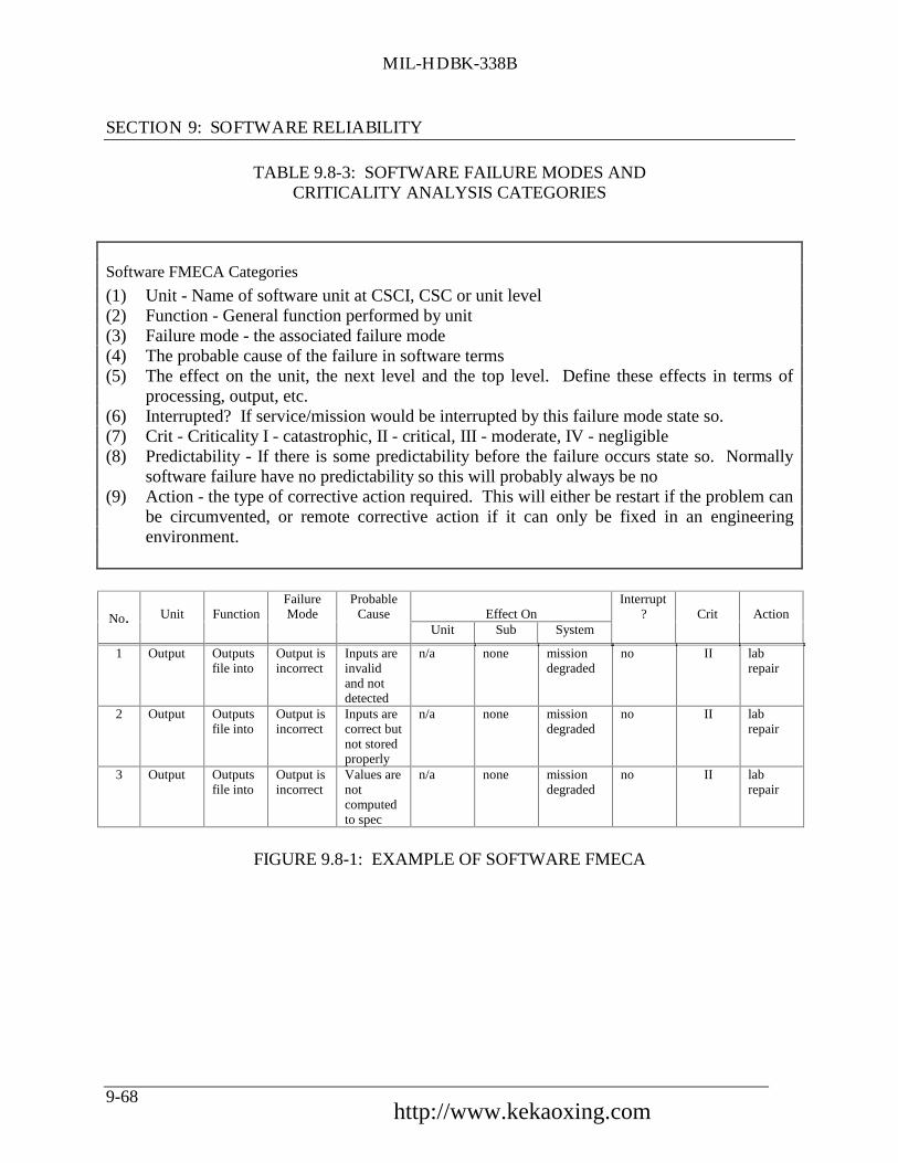
MIL-HDBK-338B


9-68

TABLE 9.8-3: SOFTWARE FAILURE MODES ANDCRITICALITY ANALYSIS CATEGORIES

Software FMECA Categories

(1) Unit - Name of software unit at CSCI, CSC or unit level(2) Function - General function performed by unit(3) Failure mode - the associated failure mode(4) The probable cause of the failure in software terms(5) The effect on the unit, the next level and the top level. Define these effects in terms of

processing, output, etc.(6) Interrupted? If service/mission would be interrupted by this failure mode state so.(7) Crit - Criticality I - catastrophic, II - critical, III - moderate, IV - negligible(8) Predictability - If there is some predictability before the failure occurs state so. Normally

software failure have no predictability so this will probably always be no(9) Action - the type of corrective action required. This will either be restart if the problem can

be circumvented, or remote corrective action if it can only be fixed in an engineeringenvironment.

Effect OnInterrupt

? ActionNo. Unit FunctionFailureMode

ProbableCause

Unit Sub SystemCrit

1 Output Outputsfile into

Output isincorrect

Inputs areinvalidand notdetected

n/a none missiondegraded

no II labrepair


Output isincorrect

Inputs arecorrect butnot storedproperly


no II labrepair


Output isincorrect

Values arenotcomputedto spec


no II labrepair

FIGURE 9.8-1: EXAMPLE OF SOFTWARE FMECA



MIL-HDBK-338B


9-69

9.9 References

1. Coppola, Anthony, “Reliability Engineering of Electronic Equipment - A HistoricalPerspective,” IEEE Transactions on Reliability, April 1984, pp. 29-35.

2. Lakey, P.B., and A.M. Neufelder, “System and Software Reliability Assurance,” RL-TR-97-XX, Rome Laboratory, 1997.

3. Jones, Capers, “Assessment and Control of Software Risks,” Yourdon, 1994.

4. Dunn, Robert, “Software Defect Removal,” McGraw-Hill, 1984.

5. Putnam, Lawrence H., and Myers, Ware, “Measures for Excellence: Reliable Software onTime, Within Budget,“ Prentice-Hill, 1992.

6. Boehm, Barry W., “Software Engineering Economics,“ Prentice-Hall, 1981.

7. Rook, Paul, Editor, “Software Reliability Handbook,” Elsevier, 1990.

8. Dyer, Michael, “The Cleanroom Approach to Quality Software Development,“ Wiley,1992.

9. Mills, Harlan D., “Cleanroom Software Engineering,” Center for Software Engineering,1994.

10. Linger, Richard C., “Cleanroom Process Model,” IEEE Software, March 1994, pp. 50-58.

11. Software Technology Support Center, “Guidelines for Successful Acquisition andManagement of Software Intensive Systems,” Dept. of the Air Force, February 1995.

12. Musa, John, A. Iannino, K. Okumoto, “Software Reliability: Measurement, Prediction,Application,“ McGraw-Hill, 1987.

13. Fairley, .R.E., “Software Engineering Concepts,“ McGraw-Hill, 1985.

14. Booch, Grady, “Object-Oriented Development,” IEEE Transactions of Software(February), 1986.

15. Meyer, Bertrand, “Object-Oriented Construction,” Prentice-Hall, 1988.

16. McCall, J.A., W. Randell, and J. Dunham, “Software Reliability, Measurement, andTesting,” Rome Laboratory, RL-TR-92-52, 1992.

MIL-HDBK-338B


9-70

17. Friedman, M.A., P.K. Tran and P.L. Goddard, “Reliability Techniques for CombinedHardware and Software Systems,” RL-TR-92-15, 1992.

18. Lloyd D.K. and M. Lipow, “Reliability: Management, Methods, and Mathematics,”Second Edition, American Society for Quality Control, 1977.

19. Farr, W.H., “A Survey of Software Reliability Modeling and Estimation,” Naval SurfaceWeapons Center, NSWC-TR-82-171, 1983.

20. Shooman, Martin L., “Software Engineering,” McGraw Hill, 1983.

21. IEEE STD 982.1, “IEEE Standard Dictionary of Measures to Produce Reliable Software,”1989.

22. IEEE STD 982.2, “Guide for the Use of IEEE Standard Dictionary of Measures to ProduceReliable Software,“ 1989.

23. Neufelder, A., “Ensuring Software Reliability,” Marcel Dekker, 1993.

24. Mahar, David, “Fault Tree Analysis,” Reliability Analysis Center (RAC), 1990.

25. Keiller, Peter A. and Douglas R. Miller, “On the Use and the Performance of SoftwareReliability Growth Models,” Software Reliability and Safety, Elsevier, 1991.

26. MIL-STD-1629A, “Procedure for Performing Failure Mode, Effects and CriticalityAnalysis,” Department of Defense, 1980.

27. Texas Instruments, Inc., “Components Sector Training and Organizational Effectiveness,Failure Modes and Effect Analysis,” 1993.



MIL-HDBK-338B

SECTION 10: SYSTEMS RELIABILITY ENGINEERING

10-1

10.0 SYSTEMS RELIABILITY ENGINEERING

10.1 Introduction

The material presented in the previous sections of this handbook in a sense set the stage for thissection. This section combines the R&M theory and engineering practices previously presentedinto a cohesive design methodology which can be applied at the system level to optimize system“worth” for minimum life cycle costs.

The “worth” of a particular equipment/system is determined primarily by the effectiveness withwhich it does its job - its “operational” effectiveness. An acceptable level of effectiveness isrequired for every operational system.

In the final analysis, the effectiveness of a system can only be really measured when the system isperforming its mission in the actual (or accurately simulated) environment for which it wasdesigned. Of critical importance, however, is how system effectiveness can be considered whilesystem design concepts are developed, how it can be ensured during design, and how it can beevaluated during test. Thus, most system effectiveness methodologies address these issues morethan measuring system effectiveness after the system is fielded.

Table 10.1-1 represents the system effectiveness concept and the parameters that have beentraditionally used (with minor variations) for system effectiveness analysis.

TABLE 10.1-1: CONCEPT OF SYSTEM EFFECTIVENESS

System Effectiveness is the Net Result ofAvailability Dependability Capability

Measures: System condition atstart of mission

System conditionduring performance ofmission

Results of mission

Determined by: Reliability

Maintainability

Human Factors

Logistics

Repairability

Safety

Survivability

Vulnerability

Range

Accuracy

Power

Lethality

etc.

MIL-HDBK-338B


10-2

As can be seen from the table, availability (how often), dependability (how long), andperformance capability (how well) are the primary measures of system effectiveness:

(1) Availability is a measure of the degree to which an item is in the operable andcommittable state at the start of the mission, when the mission is called for at anunknown (random) time.

(2) Dependability is a measure of the degree to which an item is operable and capable ofperforming its required function at any (random) time during a specified missionprofile, given item availability at the start of the mission. (This definition is differentthan the definition of dependability as it appears in International ElectrotechnicalCommission documents.)

(3) Capability is a measure of the ability of an item to achieve mission objectives, giventhe conditions during the mission.

System effectiveness assessment fundamentally answers three basic questions:

(1) Is the system working at the start of the mission?

(2) If the system is working at the start of the mission, will it continue to work during themission?

(3) If the system worked throughout the mission, will it achieve mission success?

R&M are important contributions to system effectiveness since they are significant factors inconsideration of the availability and dependability parameters. However, in the total systemdesign context, as shown in Table 10.1-1, they must be integrated with other system parameterssuch as performance, safety, human factors, survivability/vulnerability, logistics, etc., to arrive atthe optimum system configuration.

Just about all of the system effectiveness methodologies which have been developed and/orproposed in the past 20 years are concerned with this fundamental question of combining thepreviously mentioned parameters to achieve optimum system design. In Section 10.2, some ofthe more significant system effectiveness concepts and methodologies are discussed andcompared.

10.1.1 Commercial-Off-The-Shelf (COTS) and Nondevelopmental Item (NDI)Considerations

Under the current military acquisition reform initiatives, the Department of Defense isadvocating the use of Commercial-Off-The-Shelf (COTS) and Nondevelopmental Items (NDI) inthe products it acquires for military applications. Commercial industry has long used NDI inbuilding new products. NDI is any previously developed item used exclusively for governmentpurposes by “federal agency, a state or local government or a foreign government with which the



MIL-HDBK-338B


10-3

US has mutual defense cooperation agreement.”1 COTS are items available in a domestic orforeign commercial marketplace. The increased emphasis on commercial products and practiceshas occurred for a number of reasons. First, the decrease in military spending over the lastdecade has resulted in an erosion in the industrial base that existed to support development ofweapon systems. Second, while technology was driven primarily by the DoD in the past, this isno longer the case. Third, many technologies (e.g., electronics, information, communications)are advancing at such a rapid pace that the government can no longer afford an acquisitionprocess that has historically required at least a 2-3 year cycle to develop, test, and field a system.

The objective of using COTS/NDI is to reduce the development time and risk associated with anew product by reducing or eliminating new design and development, thereby capitalizing onproven designs. Whether it is the government or a private commercial company, usingCOTS/NDI can potentially reduce costs, risks, and acquisition time. However, somecompromises in the required functional performance (including reliability) of the product may benecessary, and other issues, such as logistics support, must also be considered. The decision touse COTS/NDI must be based on a thorough evaluation of its ability to perform the requiredfunction in the intended environment and to be operated and supported over the planned life ofthe product.

A product that is new in every aspect of its design carries with it cost, schedule, and performancerisks. These risks are usually high for such a product because of all the unknowns surrounding atotally new design. A product development involving a completely new design is consideredrevolutionary in nature.

In contrast to a completely new design (revolutionary approach), using a proven product orincorporating proven components and subsystems in a new product is an evolutionary approach.Using COTS/NDI is a way to follow a pattern of new product development in which new designis minimized or eliminated. Some types of NDI include:

• Items available from a domestic or foreign commercial marketplace• Items already developed and in use by the U.S. government• Items already developed by foreign governments

COTS/NDI items may constitute the entire product (e.g., a desktop computer) or they may becomponents or subsystems within the product (e.g., displays, power supplies, etc., used within acontrol system). The advantages and disadvantages of using COTS/NDI are summarized in Table10.1-2.

The use of commercial items in military systems is no longer a question of “yes or no” but aquestion of “to what degree.” A pictorial presentation of the commercial/ NDI decision processis shown in Figure 10.1-1 taken from SD-2. The R&M activities needed for COTS/NDI aredifferent than for new development items, as shown in Table 10.1-3. These considerations are 1 SD-2, Buying Commercial and Nondevelopment Item: A Handbook, Office of the Assistant Secretary ofDefense for Production and Logistics, April 1996.

MIL-HDBK-338B


10-4

discussed in more detail in the following paragraphs.

For new development programs, the customer imposes reliability requirements in the systemspecification and development specifications. (In addition, prior to Acquisition Reform, thecustomer stipulated in the statement of work which tasks the contractor would conduct as part ofthe reliability program and how (by imposing standards) the tasks were to be conducted).

With commercial items and NDI, the basic product is already designed and its reliabilityestablished. Consequently, the reliability assessment should be an operational assessment of themilitary application in the expected military environments. Since the basic design of acommercial or nondevelopmental item cannot be controlled by the buyer, the objective is todetermine whether well-established and sound reliability practices were applied during the item’sdevelopment.

When considering the use of COTS/NDI equipment, much work needs to be done up front interms of market research and development of minimum requirements. This means thatprocurement offices must work closely with the end user to define the minimum acceptableperformance specifications for R&M. Market research then needs to be performed to see whatCOTS/NDI equipment exists that has the potential of meeting defined requirements at anaffordable price.

The challenge for market research is obtaining R&M data on COTS/NDI equipment. COTSvendors may not have the kinds of data that exist in military R&M data collection systems. (Textcontinues after Tables 10.1-1 and 10.1-2 and Figure 10.1-1).



MIL-HDBK-338B


10-5

TABLE 10.1-2: ADVANTAGES AND DISADVANTAGES OF COTS/NDI

AREA OFCOMPARISON ADVANTAGES DISADVANTAGES

Technical,Schedule, andFinancial Risk

Decreased technical, financial,and schedule risks due to lessnew design of components andsubsystems. Ideally no researchand development costs areincurred.

When NDI items are used as thecomponents and subsystems of aproduct, integration of those itemsinto the product can be difficult,expensive, and time-consuming.

Performance There is increased confidence dueto established productperformance and the use ofproven components andsubsystems.

Performance trade-offs may beneeded to gain the advantages ofNDI. Integration may be difficult.

EnvironmentalSuitability

In similar applications, provenability to operate underenvironmental conditions.

In new applications, may requiremodifications external or internal tothe equipment to operate.

Leverage Ability to capitalize oneconomies of scale, state-of-the-art technology, and products withestablished quality.

There may not be a perfect matchbetween requirements and availableproducts.

Responsiveness Quick response to an operationalneed is possible because newdevelopment is eliminated orminimized.

Integration problems may reduce thetime saved.

Manufacturing If already in production,processes are probablyestablished and proven.

Configuration or process may bechanged with no advance notice.

Resupply There is no need for (large)inventory of spares because theycan be ordered from supplier.

The long-term availability of theitem(s), particularly COTS, may bequestionable.

Logistics Support No organic support may berequired (probably not possible).Repair procedures and rates areestablished.

Supplier support or innovativeintegrated logistics support strategiesmay be needed to support theproduct.

MIL-HDBK-338B


10-6

TABLE 10.1-3: R&M ACTIVITIES FOR NEW DEVELOPMENTITEMS AND FOR COTS

TYPE OF ITEMR&M ACTIVITY NEW DEVELOPMENT COTS/NDI

DetermineFeasibility

Develop requirements based onuser needs and technology beingused. Estimate achievable level ofR&M.

Limited to verifying manufacturerclaims.

Understand theDesign

Perform FMEA, FTA, and otheranalyses for entire design. Conductdesign reviews. Develop deratingcriteria. Conduct developmenttesting.

Limited to integration and anymodifications.

Parts Selection Analyze design to determinecorrect parts application for robustdesign. Identify needed screening.

None.

Validate the Design Conduct extensive developmenttesting that addresses all aspects ofthe design. Identify designdeficiencies and take correctiveaction. Establish achieved levels ofR&M.

Limited to what is needed to verifymanufacturer claims and to validateintegration or requiredmodifications based on theintended environment.

Manufacturing Design manufacturing processes toretain inherent R&M. Implementstatistical process control anddevelop good supplierrelationships.

None if the item is already inproduction. Otherwise, design themanufacturing process to retain theinherent design characteristics.



MIL-HDBK-338B


10-7

Conductmarket

investigation

Is amaterial solution

needed?

Identify anoperational

need

Isthere anexistingsystem?

Use or modifythe existing

system

Use anon-material

solution

Evaluate:- Performance- Life cycle cost- Integrated Logistics Support

Issue Requestfor Proposal

orInvitation

for Bid

Is acommercial item

feasible?

Is anNDI feasible?

Go to adevelopment

program

Yes

No

No

YesSelectcommercial

or NDI solution

Consider commercial andnondevelopmental itemsfor subsystems andcomponents.

Yes

Yes*No

No

* In preparation for the market investigation establish objectives and thresholds for cost, schedule, and performancebased on the users’ operational and readiness requirements.

FIGURE 10.1-1: THE COMMERCIAL/NDI DECISION PROCESS

MIL-HDBK-338B


10-8

If design documentation is available, specific R&M tasks, such as prediction and failure modesand effects analysis, may be part of the COTS/NDI evaluation process. Because the primemilitary contractor is not likely to be the COTS/NDI vendor in this case, both the governmentand the prime will need to perform the evaluation i.e., a cooperative effort should exist betweenthe two parties.

The amount of testing required to verify that a commercial item or NDI meets the operationalrequirement is governed by whether the item will be used in the environment for which it wasdesigned and by operators with skills equal to the operators for which it was designed. Whatmay be needed is to require the supplier to furnish operational and environmentalcharacterization data and the results of testing to substantiate reliability and maintainabilityclaims. Also, it may be necessary to require the supplier provide some evidence that themanufacturing processes do not compromise the designed-in reliability and maintainabilitycharacteristics. This evidence may include the results of sampling tests, control charts showingthat critical processes are in control with a high process capability, and so forth.

10.1.2 COTS/NDI as the End Product

When purchasing COTS/NDI as the total product, the best course of action may be to requireonly data that substantiates R&M performance claims and to emphasize the role of themanufacturing processes (for NDI not yet in production) in determining the reliability andmaintainability of the product. In some cases, even that data may not be needed if either thecustomer has already determined (through its own testing of samples, for example) that theproduct has the requisite performance, or if use or independent testing of the product incommercial applications has shown the product’s performance to be satisfactory (for example, apersonal computer in an office environment). In any case, imposing specific R&M tasks onmanufacturers of COTS/NDI, even if they were willing to bid on such a procurement, is usuallycounterproductive and expensive.

The advantage of using COTS/NDI is that the development is complete (with only minorexceptions); the supplier has already done (or omitted) whatever might have been done to designa reliable and maintainable product. What may be need is to require the supplier to furnishoperational and environmental characterization data and the results of testing to substantiatereliability and maintainability claims. Also, it may be necessary to require the supplier providesome evidence that the manufacturing processes do not compromise the designed-in reliabilityand maintainability characteristics. This evidence may include the results of sampling tests,control charts showing that critical processes are in control with a high process capability, and soforth.

10.1.3 COTS/NDI Integrated with Other Items

When COTS/NDI is being integrated with other items, either new development or otherCOTS/NDI, the same attention and level of effort that is characteristic of a new developmentmust be given to the integration. R&M and other performance characteristics may be seriously



MIL-HDBK-338B


10-9

affected by the integration due to feedback, interference and other interactions. The integrationmay require interface devices, which themselves may present new R&M problems. One wouldexpect a supplier to perform Failure Modes and Effects Analysis (FMEA), Fault Tree Analysis(FTA), and other analyses to ensure that the integration does not compromise the R&Mperformance of any of the items being integrated and that the resulting product meets the requiredlevels of R&M performance.

10.1.4 Related COTS/NDI Issues

Three of the most important issues associated with using COTS/NDI are the logistics supportconcept, availability of parts, and performance in the intended military environment. Otherissues include configuration management of the COTS/NDI (important if the customer plans tosupport the product organically), and the availability or development of documentation to supportoperations and organic maintenance.

10.2 System Effectiveness Concepts

The three generally recognized components of system effectiveness previously defined(availability, dependability, capability) will be used as the basis for description and comparisonof the concepts and formulations of system effectiveness. It should be recognized that all ofthese effectiveness components must be derived from an analysis of the operational needs andmission requirements of the system, since it is only in relation to needs and missions that thesebasic components can be meaningfully established.

Many semantic difficulties arise when discussing systems effectiveness and its components.These difficulties result from the fact that some people use the same words to mean differentthings or different words to mean the same things.

Definitions of many of the terms used in the following paragraphs were provided in Section 3and will not be repeated here.

10.2.1 The ARINC Concept of System Effectiveness (Ref. [1])

One of the early attempts to develop concepts of system effectiveness was delineated by ARINC(Aeronautical Radio Inc.) in its book “Reliability Engineering.” It contains some of the earliestpublished concepts of systems effectiveness and represents one of the clearest presentations ofthese concepts from which many of the subsequent descriptions have been derived. Thedefinition of systems effectiveness applied in this early work is: “Systems effectiveness is theprobability that the system can successfully meet an operational demand within a given timewhen operated under specified conditions.” This definition includes the concepts that systemeffectiveness

(1) Can be measured as a probability

MIL-HDBK-338B


10-10

(2) Is related to operation performance

(3) Is a function of time

(4) Is a function of the environment or conditions under which it is used

(5) May vary with the mission to be performed

Although it is not essential to describe system effectiveness in terms of probability as opposed toother quantitative measures, it has often been found convenient to do so. The ARINC modelmay be expressed such that system effectiveness probability, PSE, is the product of threeprobabilities as follows:

PSE = POR • PMR • PDA (10.1)

where:POR = operational readiness probability

PMR = mission reliability probability

PDA = design adequacy probability

This equation states that the effectiveness of the system is the product of three probabilities: (1)the probability that the system is operating satisfactorily or is ready to be placed in operationwhen needed; (2) the probability that the system will continue to operate satisfactorily for theperiod of time required for the mission; and (3) the probability that the system will successfullyaccomplish its mission, given that it is operating within design limits.

10.2.2 The Air Force (WSEIAC) Concept (Ref. [2])

A later definition of system effectiveness resulted from the work of the Weapon SystemEffectiveness Industry Advisory Committee (WSEIAC) established in late 1963 by the Air ForceSystem Command. The WSEIAC definition of system effectiveness is: “System effectiveness isa measure of the extent to which a system may be expected to achieve a set of specific missionrequirements and is a function of availability, dependability, and capability.” The definition maybe expressed as:

SE = ADC (10.2)



MIL-HDBK-338B


10-11

where:A = availabilityD = dependabilityC = capability

See definitions in Section 10.1.

These are usually expressed as probabilities as follows:

(1) “A” is the vector array of various state probabilities of the system at the beginning ofthe mission.

(2) “D” is a matrix of conditional probabilities over a time interval, conditional on theeffective state of the mission during the previous time interval.

(3) “C” is also a delineal probability matrix representing the performance spectrum of thesystem, given the mission and system conditions, that is, the expected figures of meritfor the system.

Basically, the model is a product of three matrices:

• Availability row vector A

• Dependability matrix D

• Capability matrix C

In the most general case, assume that a system can be in different states and at any given point intime is in either one or the other of the states. The availability row vector is then

A = (a1 , a2 , a3 , . . ., ai , . . . an ) (10.3)

where ai is the probability that the system is in State i at a random mission beginning time.

Since the system can be in only one of the n states and n is the number of all possible states it canbe in (including the down states in which the system cannot start a mission), the sum of all theprobabilities ai in the row vector must be unity, i.e.,

∑i=1

n ai = 1 (10.4)

MIL-HDBK-338B


10-12

The dependability matrix D is defined as a square n • n matrix

D =

d11 d12 d13 . . . . d1nd21 d22 d23 . . . . d2n. .. .. .dn1 dn2 dn3 . . . . dnn

(10.5)

where the meaning of the element dij is defined as the expected fraction of mission time during

which the system will be in State j if it were in State i at the beginning of the mission. If systemoutput is not continuous during the mission but is required only at a specific point in the mission(such as over the target area), dij is defined as the probability that the system will be in State j at

the time when output is required if it were in State i at mission start.

When no repairs are possible or permissible during a mission, the system upon failure or partialfailure cannot be restored to its original state during the mission and can at best remain in theState i in which it started the mission or will degrade into lower states or fail completely. In thecase of no repairs during the mission, some of the matrix elements become zero. If we defineState 1 as the highest state (i.e., everything works perfectly) and n the lowest state (i.e., completefailure), the dependability matrix becomes triangular with all entries below the diagonal beingzeros.

D =

d11 d12 d13 . . d1n

0 d22 d23 . . d2n. . . . . .. . . . . .. . . . . .0 0 0 . . dnn

(10.6)

If the matrix is properly formulated the sum of the entries in each row must equal unity. Forexample, for the first row we must have

d11 + d12 + . . . + d1n = 1 (10.7)

and the same must apply to each subsequent row. This provides a good check when formulatinga dependability matrix.

The capability matrix, C, describes system performance or capability to perform while in any of



MIL-HDBK-338B


10-13

the n possible system states. If only a single measure of system effectiveness is of importance orof interest, C will be a one column matrix with n elements, such as

C =

c1c2...

cn

(10.8)

where cj represents system performance when the system is in State j.

System effectiveness, SE, in the WSEIAC model is then defined as

SE = a1, a2, ..., an[ ] •

d11 d12 . . . d1n

d21 d22 . . . d2n. .. .. .

dn1 dn2 . . . dnn

•

C1C2...

Cn

(10.9)

= ∑i=1

n ∑

j=1

n ai • dij • cj (10.10)

Reference [2] contains several numerical examples of how to perform system effectivenesscalculations using the WSEIAC model. Also, Ref. [3], Chapter VII, discusses the model atlength and provides numerical examples.

MIL-HDBK-338B


10-14

10.2.3 The Navy Concept of System Effectiveness (Ref. [4])

In the early 1960’s, the Navy developed a system effectiveness concept which also combinesthree basic system characteristics: performance, availability and utilization. It can be expressedas “a measure of the extent to which a system can be expected to complete its assigned missionwithin an established time frame under stated environmental conditions.” It may also be definedmathematically as “the probability that a system can successfully meet an operational demandthrough a given time period when operated under specified conditions.”

Mathematically it has been formulated as follows:

ES = PAU (10.11)

where:ES = index of system effectiveness

P = index of system performance - a numerical index expressing system capability,assuming a hypothetical 100% availability and utilization of performancecapability in actual operation

A = index of the system availability - a numerical index of the extent to which thesystem is ready and capable of fully performing its assigned mission(s)

U = index of system utilization - a numerical index of the extent to which theperformance capability of the system is utilized during the mission

The components of the Navy model are not as readily computed as are those of the ARINC andWSEIAC models. The Navy has stated that the terms PU and A are similar to the WSEIACterms C and AD (Ref. [5]) and that PAU can be translated into the analytical terms PC and PT

where:PC performance capability - a measure of adequacy of design and system

degradationPT detailed time dependency - a measure of availability with a given

utilization

Thus the Navy model is compatible with the WSEIAC model in the following way:

f(PAU) = f(PC , PT ) = f(A,D,C) (10.12)

The WSEIAC, Navy and ARINC concepts of system effectiveness are depicted in Figure 10.2-1.



MIL-HDBK-338B


10-15

DESIGN ADEQUACY

PROBABILITY THAT ASYSTEM WILL SUCCESS-FULLY ACCOMPLISH ITSMISSION GIVEN THATTHE SYSTEM IS OPERAT-ING WITHIN DESIGNSPECIFICATIONS

MISSION RELIABILITY

PROBABILITY OF ASYSTEM PERFORMINGITS PURPOSEADEQUATELY FORTHE PERIOD OF TIMEINTENDED

OPERATIONAL READINESS

PROBABILITY THAT ATANY POINT IN TIME ASYSTEM IS OPERATINGSATISFACTORILY OR ISREADY TO BE PLACED INOPERATION ON DEMAND

SYSTEM EFFECTIVENESS (SE)

(A) ARINC MODEL

CAPABILITY (C)

MEASURE OF RESULTSOF MISSION

DEPENDABILITY (D)

MEASURE OF SYSTEMCONDITION DURING PER-FORMANCE OF MISSION

AVAILABILITY (A)

MEASURE OF SYSTEMCONDITION AT STARTOF MISSION


(B) WSEIAC MODEL

UTILIZATION (U)

TACTICALENVIRONMENTALFUNCTIONALLOGISTICAL

AVAILABILITY (A)

MAN-MACHINE MODULES

RELIABILITYMAINTAINABILITYOPERABILITYLOGISTICS SUPPORTABILITYSAFETY

PERFORMANCE (P)

ACHIEVED PERFORMANCEDESIRED PERFORMANCE

PRIMARY MISSIONSECONDARY MISSIONNO MISSION

FRACTIONS OF TOTALMISSION TIME


(C) NAVY MODEL

RANGEACCURACYPOWERLETHALITY

REPAIRABILITYSAFETYFLEXIBILITYSURVIVABILITY

RELIABILITYHUMAN FACTORSMAINTAINABILITYLOGISTIC SUPPORT

RELIABILITYHUMAN FACTORSMAINTAINABILITYLOGISTIC SUPPORT

FIGURE 10.2-1: SYSTEM EFFECTIVENESS MODELS

MIL-HDBK-338B


10-16

Although these models are relatively simple to describe, their development and application is arather complex process usually performed by operations research groups and operations analystsutilizing available computerized models (to be discussed later).

10.2.4 An Illustrative Model of a System Effectiveness Calculation

The following simplified example, utilizing the WSEIAC concept, is provided in order to showhow R&M parameters are used in system effectiveness calculations.

Problem Statement

The system to be considered consists of a helicopter and its communication equipment. It is tooperate in a limited warfare environment where rapid movement of supplies upon request isimportant. The mission of the system is that upon random call of transporting supplies from acentral supply to operational activities within a radius of one-half hour flying time and providingvertical underway replenishment of needed spares. Once the helicopter has reached the targetarea, proper functioning of the communication equipment enhances the chances of a successfuldelivery of the supplies in terms of safe delivery, timely delivery, etc. Some major assumptionswhich are inherent in this example are:

(1) A call for supplies is directed to a single helicopter. If this craft is not in flyablecondition (i.e., it is in process of maintenance), the mission will not be started. Aflyable craft is defined as one which is in condition to take off and fly with a standardsupply load.

(2) The flight time required to reach the target area is one-half hour.

(3) The communication equipment cannot be maintained or repaired in flight.

(4) A loaded helicopter which goes down while enroute to, or which does not reach, thetarget area, has no delivery value.

Model Determination

For purposes of model formulation, the system condition is divided into three states:

(1) State 1:Helicopter flyable, communication equipment operable

(2) State 2:Helicopter flyable, communication equipment nonoperable

(3) State 3:Helicopter nonflyable



MIL-HDBK-338B


10-17

The WSEIAC model for effectiveness is given by the following equation:

SE = ADC

where A, D and C are defined as follows:

(1) The availability vector is a three-element, row vector, i.e.,

A = (a1 , a2 , a3 )

where ai is the probability that the helicopter will be in State i at the time of call.

(2) The dependability matrix is a 3x3 square matrix, i.e.,

D =

d11 d12 d13d21 d22 d23d31 d32 d33

where dij is the probability that if the helicopter is in State i at the time of call it will

complete the mission in State j.

(3) The capability vector is a three-element column vector, i.e.,

C =

c1c2c3

where ci is the probability that if the helicopter is in State i at the time of arrival at the

target area the supplies can be successfully delivered. (For multi-capability items, Cwould be a multi-column matrix.)

MIL-HDBK-338B


10-18

Determination of Model Elements

Past records indicate that the average time between maintenance activities (including preventiveand failure initiated maintenance) for this type of helicopter is 100 hours and the averageduration (including such variables as maintenance difficulty, parts availability, manpower, etc.)of a maintenance activity is ten hours. Comparable data for the communication equipment showsan average time between maintenance activities of 500 hours and an average duration of amaintenance activity of five hours.

From the preceding data the elements of A can be determined.

A1 = P(helicopter flyable) • P(communication equipment operable)

=

100

100 + 10

500

500 + 5 = 0.9

A2 = P(helicopter flyable) • P(communication equipment not operable)

=

100

100 + 10

5

500 + 5 = 0.009

A3 = P(helicopter not flyable) =

10

100 + 10 = 0.091

Data from past records indicates that the time between failures of the communication equipmentduring flight is exponentially distributed with a mean of 500 hours. Also, the probability that ahelicopter in flight will not survive the one-half hour flight to its destination is 0.05 (includesprobability of being shot down, mechanical failures, etc.). Then the elements of the D matrixmay be calculated as follows:

(1) If the system begins in State 1:

d11 = P(helicopter will survive flight) • P(communication equipment will

remain operable)

= (1 - 0.05) exp

-

1/2500 = 0.94905

d12 = P(helicopter will survive flight) • P(communication equipment will

fail during flight)

= (1 - 0.05)

1 - exp

-

1/2500 = 0.00095



MIL-HDBK-338B


10-19

d13 = P(helicopter will not survive the flight) = 0.05000


d21 = 0 because the communication equipment cannot be repaired in

flight

d22 = P(helicopter will survive flight) = 0.95000

d23 = P(helicopter will not survive the flight) = 0.05000


d31 = d32 = 0 because the mission will not start

d33 = 1, i.e., if the helicopter is not flyable, it will remain nonflyable with

reference to a particular mission

Experience and technical judgment have determined the probability of successful delivery ofsupplies to be ci if the system is in State i at the time of arrival in the target area, where

c1 = 0.95 c2 = 0.80 c3 = 0

Determination of Effectiveness

The effectiveness of the subject system becomes

E =

0.900 0.009 0.091

0.94905 0.00095 0.050 0.95 0.050 0 1

0.950.80

= 0.82

which means that the system has a probability of 0.82 of successful delivery of supplies uponrandom request.

The effectiveness value attained provides a basis for deciding whether improvement is needed.The model also provides the basis for evaluating the effectiveness of alternative systemsconsidered.

MIL-HDBK-338B


10-20

10.3 System R&M Parameters

In this section we are concerned with those system effectiveness submodels, e.g., availability,dependability, operational readiness, which can be exercised to specify, predict, allocate,optimize, and measure system R&M parameters.

Four types of parameters and examples of specific R&M terms applicable to their specificationand measurement, are shown in Table 10.3-1. Each will be discussed in more detail in thefollowing paragraphs.

TABLE 10.3-1: SYSTEM R&M PARAMETERS

OBJECTIVES EXAMPLE TERMS

• READINESS OR AVAILABILITY R: Mean Time Between Downing EventsM: Mean Time to Restore System

• MISSION SUCCESS R: Mission Time Between Critical FailuresM: Mission Time to Restore Function

• MAINTENANCE MANPOWER COST R: Mean Time Between Maintenance ActionsM: Direct Man-hours per Maintenance Action

• LOGISTIC SUPPORT COST R: Mean Time Between RemovalsM: Total Parts Cost per Removal

Operational Readiness R&M Parameters - These parameters will define the R&M contribution tothe readiness measurement of the system or unit. R&M by itself does not define readiness; thereare many other factors relating to personnel, training, supplies, etc., that are necessarily includedin any real measure of readiness. The context of readiness includes many factors beyond therealm of equipment capability and equipment R&M achievements. R&M parameters of this typeconcern themselves with the likelihood of failures occurring that would make a ready system nolonger ready and with the effort required to restore the system to the ready condition. Examplesof this type of parameter are “mean time between downing events” for reliability and “mean timeto restore system” for maintainability.

Mission Success R&M Parameters - These parameters are similar to the classical reliabilitydiscussion that is found in most reliability text books. They relate to the likelihood of failuresoccurring during a mission that would cause a failure of that mission and the efforts that aredirected at correcting these problems during the mission itself. Examples would be “missiontime between critical failures (MTBCF)” for reliability and “mission time to restore function” formaintainability.

Maintenance Manpower Cost R&M Parameters - Some portion of a system's maintenancemanpower requirement is driven by the system's R&M achievement. This category of systemR&M parameters concerns itself with how frequently maintenance manpower is required and,



MIL-HDBK-338B


10-21

once it is required, how many man-hours are needed. Examples of this type of parameter are“mean time between maintenance actions” for reliability and “direct man-hours to repair” formaintainability. Note that the maintainability example does not address the clock hours tocomplete the repair. Time to restore the system, i.e., the system downtime, is not as significant tothe people concerned with manpower needs as the total man-hours required.

Logistic Support Cost R&M Parameters - In many systems, this type of R&M parameter mightbe properly titled as “material cost” parameters. These parameters address the aspect of R&Machievement that requires the consumption of material. Material demands also relate to thereadiness or availability of the system. Examples are “mean time between removals” forreliability and “total parts cost per removal” for maintainability.

Let us examine some of the techniques for using reliability data, reduced to parameters such asthose just discussed, for making reliability predictions.

10.3.1 Parameter Translation Models

Frequently it is necessary to convert various reliability parameters from one set of environmentalconditions to a different set of environmental conditions. Extensive reliability data may havebeen generated or gathered in a given environment while the equipment may be subsequentlyslated for use in an entirely different environment. In other cases, the customers may define areliability parameter differently than the manufacturer does, or he may use an entirely differentfigure-of-merit as the basis for acceptance. The intent of this section is to address these areas ofconcern.from:kekaoxing.com

10.3.1.1 Reliability Adjustment Factors

“What if” questions are often asked regarding reliability figures of merit for different operatingconditions. For example, what reliability could be expected from a product in a ground fixedenvironment that is currently experiencing a 700 hour MTBF in an airborne environment. Tableshave been derived to make estimates of the effects of quality levels, environments andtemperatures enabling rapid conversions between environments. The database upon which thesetables are based was a grouping of approximately 18,000 parts from a number of equipmentreliability predictions performed on various military contracts. Ratios were developed using thisdatabase and the MIL-HDBK-217F algorithms. The relative percentages of each part type in thedatabase are shown in Figure 10.3-1.

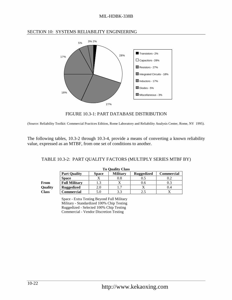
MIL-HDBK-338B


10-22

2%

28%

27%

18%

17%

5%3%

Transistors - 2%

Capacitors - 28%

Resistors - 27%

Integrated Circuits - 18%

Inductors - 17%

Diodes - 5%

Miscellaneous - 3%

FIGURE 10.3-1: PART DATABASE DISTRIBUTION

(Source: Reliability Toolkit: Commercial Practices Edition, Rome Laboratory and Reliability Analysis Center, Rome, NY 1995).

The following tables, 10.3-2 through 10.3-4, provide a means of converting a known reliabilityvalue, expressed as an MTBF, from one set of conditions to another.

TABLE 10.3-2: PART QUALITY FACTORS (MULTIPLY SERIES MTBF BY)

To Quality ClassPart Quality Space Military Ruggedized CommercialSpace X 0.8 0.5 0.2

From Full Military 1.3 X 0.6 0.3Quality Ruggedized 2.0 1.7 X 0.4Class Commercial 5.0 3.3 2.5 X

Space - Extra Testing Beyond Full MilitaryMilitary - Standardized 100% Chip TestingRuggedized - Selected 100% Chip TestingCommercial - Vendor Discretion Testing



MIL-HDBK-338B


10-23

TABLE 10.3-3: ENVIRONMENTAL CONVERSION FACTORS (MULTIPLY SERIES MTBF BY)

To EnvironmentGB GF GM NS NU AIC AIF AUC AUF ARW SF

GB X 0.5 0.2 0.3 0.1 0.3 0.2 0.1 0.1 0.1 1.2

GF 1.9 X 0.4 0.6 0.3 0.6 0.4 0.2 0.1 0.2 2.2

GM 4.6 2.5 X 1.4 0.7 1.4 0.9 0.6 0.3 0.5 5.4

FromNS 3.3 1.8 0.7 X 0.5 1.0 0.7 0.4 0.2 0.3 3.8

Environment NU 7.2 3.9 1.6 2.2 X 2.2 1.4 0.9 0.5 0.7 8.3

AIC 3.3 1.8 0.7 1.0 0.5 X 0.7 0.4 0.2 0.3 3.9

AIF 5.0 2.7 1.1 1.5 0.7 1.5 X 0.6 0.4 0.5 5.8

AUC 8.2 4.4 1.8 2.5 1.2 2.5 1.6 X 0.6 0.8 9.5

AUF 14.1 7.6 3.1 4.4 2.0 4.2 2.8 1.7 X 1.4 16.4

ARW 10.2 5.5 2.2 3.2 1.4 3.1 2.1 1.3 0.7 X 11.9

SF 0.9 0.5 0.2 0.3 0.1 0.3 0.2 0.1 0.1 0.1 X

Environmental Factors as Defined in MIL-HDBK-217

GB - Ground Benign; GF - Ground Fixed; GM - Ground Mobile; NS - Naval Sheltered; NU - Naval Unsheltered; AIC -Airborne Inhabited Cargo; AIF - Airborne Inhabited Fighter; AUC - Airborne Uninhabited Cargo; AUF - Airborne UninhabitedFighter; ARW - Airborne Rotary Winged; SF - Space Flight

CAUTION: Do not apply to MTBCF.

MIL-HDBK-338B


10-24

TABLE 10.3-4: TEMPERATURE CONVERSION FACTORS (MULTIPLY SERIES MTBF BY)

To Temperature (°C)Temp. 10 20 30 40 50 60 7010 X 0.9 0.8 0.8 0.7 0.5 0.420 1.1 X 0.9 0.8 0.7 0.6 0.530 1.2 1.1 X 0.9 0.8 0.6 0.5

From Temperature 40 1.3 1.2 1.1 X 0.9 0.7 0.6(°C) 50 1.5 1.4 1.2 1.1 X 0.8 0.7

60 1.9 1.7 1.6 1.5 1.2 X 0.870 2.4 2.2 1.9 1.8 1.5 1.2 X

10.3.1.2 Reliability Prediction of Dormant Products

In the past, analysis techniques for determining reliability estimates for dormant or storageconditions relied on simple rules of thumb such as: “the failure rate will be reduced by a ten toone factor”, or “the expected failure rate is zero.” A more realistic estimate, based on part countfailure results, can be calculated by applying the conversion factors shown for the example inTable 10.3-5. The factors convert operating failure rates by part type to dormant conditions forseven scenarios.

These conversion factors were determined using data from various military contracts andalgorithms from both MIL-HDBK-217F and RADC-TR-85-91, “Impact of Nonoperating Periodson Equipment Reliability” (Ref. [34]). Average values for operating and dormant failure rateswere developed for each scenario. For example, to convert the reliability of an operatingairborne receiver to a ground nonoperating condition, determine the number of components bytype, then multiply each by the respective operating failure rate obtained from handbook data,field data, or vendor estimates. The total operating failure rate for each type is then convertedusing the conversion factors of Table 10.3-5. The dormant estimate of reliability for the examplereceiver is determined by summing the part results.



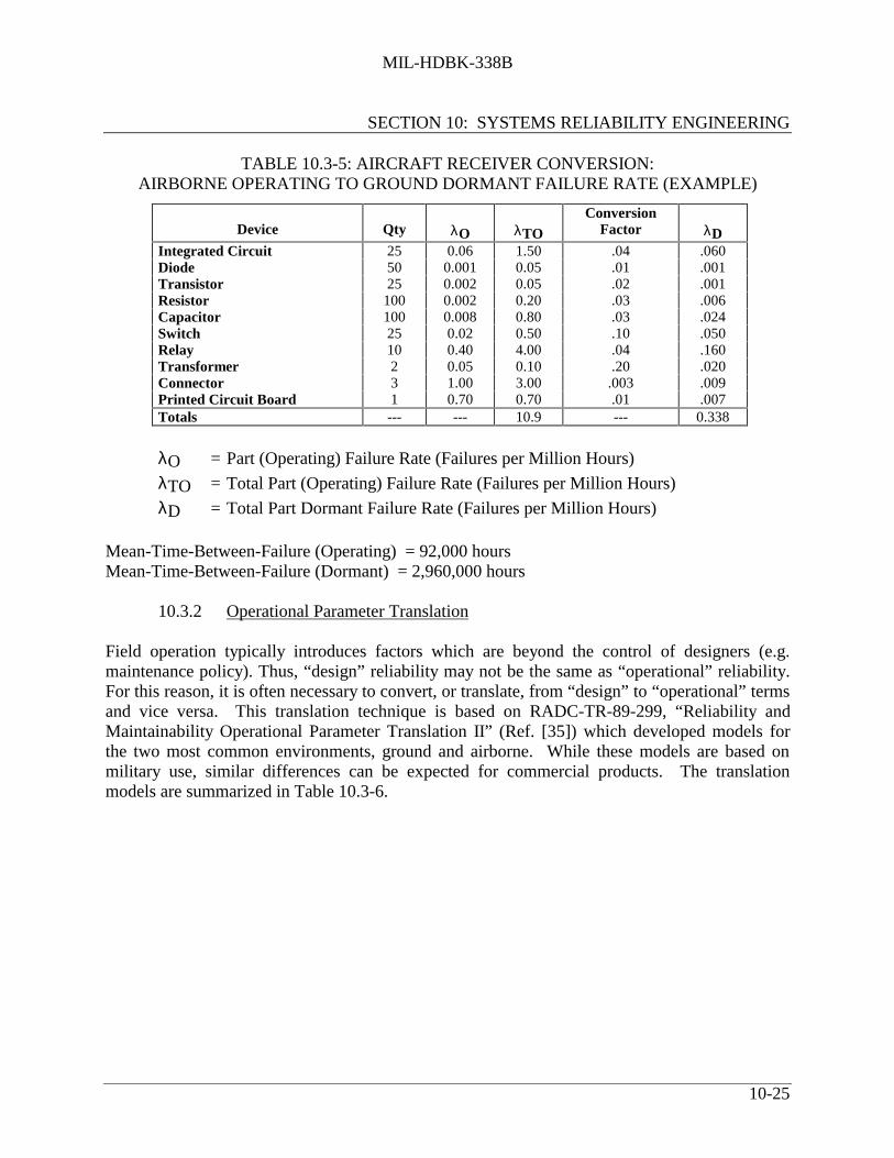
MIL-HDBK-338B


10-25

TABLE 10.3-5: AIRCRAFT RECEIVER CONVERSION:AIRBORNE OPERATING TO GROUND DORMANT FAILURE RATE (EXAMPLE)

Device Qty λO λTOConversion

Factor λDIntegrated Circuit 25 0.06 1.50 .04 .060Diode 50 0.001 0.05 .01 .001Transistor 25 0.002 0.05 .02 .001Resistor 100 0.002 0.20 .03 .006Capacitor 100 0.008 0.80 .03 .024Switch 25 0.02 0.50 .10 .050Relay 10 0.40 4.00 .04 .160Transformer 2 0.05 0.10 .20 .020Connector 3 1.00 3.00 .003 .009Printed Circuit Board 1 0.70 0.70 .01 .007Totals --- --- 10.9 --- 0.338

λO = Part (Operating) Failure Rate (Failures per Million Hours)

λTO = Total Part (Operating) Failure Rate (Failures per Million Hours)

λD = Total Part Dormant Failure Rate (Failures per Million Hours)

Mean-Time-Between-Failure (Operating) = 92,000 hoursMean-Time-Between-Failure (Dormant) = 2,960,000 hours

10.3.2 Operational Parameter Translation

Field operation typically introduces factors which are beyond the control of designers (e.g.maintenance policy). Thus, “design” reliability may not be the same as “operational” reliability.For this reason, it is often necessary to convert, or translate, from “design” to “operational” termsand vice versa. This translation technique is based on RADC-TR-89-299, “Reliability andMaintainability Operational Parameter Translation II” (Ref. [35]) which developed models forthe two most common environments, ground and airborne. While these models are based onmilitary use, similar differences can be expected for commercial products. The translationmodels are summarized in Table 10.3-6.

MIL-HDBK-338B


10-26

TABLE 10.3-6: RELIABILITY TRANSLATION MODELS

RF Selection

Communication Navigation ComputerCounterMeasure Radar All Other

Dependent Var.Lower Bound (%

of Ind. Var.)*1. Airborne Fighter Models

1A. MTBFF = θP.64RF ( )

CD -.46

2.1 6.5 5.9 4.7 3.6 4.3 48

1B. MTBMF = θP.64 RF ( )

CD

-.571.1 2.7 1.9 2.8 1.7 2.0 24

1C. MTBRF = θP.62 RF ( )

CD -.77

1.8 4.4 3.0 5.9 2.5 3.2 34

1D. MTBFF = θD.76 RF ( )

CD -.34

2.1 5.0 5.3 3.7 5.1 2.2 79

1E. MTBMF = θD.75 RF ( )

CD -.44

1.4 2.2 1.8 2.4 2.8 .90 36

1F. MTBRF = θD.77 RF ( )

CD -.65

1.6 4.0 2.2 3.4 3.0 .83 49

2. Airborne Transport Models RF, Uninhabited Equipment RF, Inhabited Equipment

2A. MTBFF = θP.73 RF ( )

CD -.46 2.7 2.5 50

2B. MTBMF = θP.69 RF ( )

CD -.57 1.6 1.4 26

2C. MTBRF = θP.66 RF ( )

CD -.77 2.1 2.3 35

2D. MTBFF = θD1.0 RF ( )

CD

-.34 .58 .39 91

2E. MTBMF = θD1.1 RF ( )

CD -.44 .13 .09 44

2F. MTBRF = θD.88 RF ( )

CD

-.65 .78 .60 72

3. Ground System Models RF, Fixed Equipment RF, Mobile Equipment

3A. MTBFF = θP.60 RF

27 4.8 90

3B. MTBMF = θP.67 RF

11 1.8 49

3C. MTBRF = θP.50 RF

91 18 80

*The field numeric (i.e., MTBFF, MTBMF or MTBRF) is always taken to be the lesser of (1) the calculated valuefrom Column 1 or, (2) the percentage shown of the independent variable (i.e., θP or θD).



MIL-HDBK-338B


10-27

10.3.2.1 Parameter Definitions

• Mean-time-between-failure-field (MTBFF) includes inherent maintenance events whichare caused by design and manufacturing defects.

MTBFF = Total Operating Hours or Flight Hours

Inherent Maintenance Events

• Mean-time-between-maintenance-field (MTBMF) consists of inherent, induced and nodefect found maintenance actions.

MTBMF = Total Operating Hours or Flight Hours

Total Maintenance Events

• Mean-time-between-removals-field (MTBRF) includes all removals of the equipmentfrom the system.

MTBRF = Total Operating Hours or Flight Hours

Total Equipment Removals

• θP = the predicted MTBF (i.e., estimated by failure rates of the part

population)• θD = the demonstrated MTBF (i.e., controlled testing)

• RF = the equipment type or application constant

• C = the power on-off cycles per mission or operating event• D = the mission duration or operating event

10.3.2.2 Equipment Operating Hour to Flight Hour Conversion

For airborne categories - MTBFF represents the mean-time-between-failure in equipmentoperating hours. To obtain MTBFF in terms of flight hours (for both fighter and transportmodels), divide MTBFF by 1.2 for all categories except countermeasures. Divide by .8 forcountermeasures equipment.

Example 1:

Estimate the MTBM of a fighter radar given a mission length of 1.5 hours, two radar shutdownsper mission and a predicted radar MTBF of 420 hours. Using Model 1B in Table 10.3-6,

MTBMF = θP

.64 R

F

C

D - .57 = (420 hr.).64

1.7

2 cyc. 1.5 hr.

- .57

MTBMF = 69 equipment operating hours between maintenance.

MIL-HDBK-338B


10-28

Since this is below the dependent variable lower bound of (.24)(420) = 101 hours, the calculatedMTBMF is correct. Since this equipment is often turned on for pre- and post-flight checkout,

the number of flight hours between maintenance is somewhat less than the actual equipmentoperating hours. The number of flight hours between maintenance is approximately 69/1.2 = 58hours.

Example 2:

Estimate the MTBF of a commercial airline navigation unit used on an 8 hour flight and shutdown after the flight. The predicted MTBF for the navigation unit is 2,000 hours. Using model2A for inhabited environment,

MTBFF = θP.73 RF

C

D-.46

= (2,000).73 2.5

1 cycle

8 hours-.46

MTBFF = 1,672 hours between failure

The number of flight hours between failure is estimated to be 1,672/1.2 = 1,393 hours. However,in accordance with the footnote of Table 10.3-6, we calculate a value of (.50)(2000) = 1000 hoursusing the dependent variable bound. Since this is less than the previous calculation, this is thevalue to be used.

10.3.3 Availability, Operational Readiness, Mission Reliability, andDependability - Similarities and Differences

As can be seen from their definitions in Table 10.3-7, availability and operational readiness referto the capability of a system to perform its intended function when called upon to do so. Thisemphasis restricts attention to probability “at a point in time” rather than “over an interval oftime.” Thus, they are point concepts rather than interval concepts. To differentiate between thetwo: availability is defined in terms of operating time and downtime, where downtime includesactive repair time, administrative time, and logistic time; whereas, operational readiness includesall of the availability times plus both free time and storage time, i.e., all calendar time.



MIL-HDBK-338B


10-29

TABLE 10.3-7: DEFINITIONS OF KEY R&M SYSTEM PARAMETERS

AVAILABILITY: A measure of the degree to which an item is in an operable and committable state at thestart of a mission when the mission is called for at an unknown (random) time. (Item state at start of amission includes the combined effects of the readiness-related system R&M parameters but excludesmission time.)

OPERATIONAL READINESS: The ability of a military unit to respond to its operation plan(s) uponreceipt of an operations order. (A function of assigned strength, item availability, status or supply, training,etc.)

MISSION RELIABILITY: The ability of an item to perform its required functions for the duration of aspecified "mission profile."

DEPENDABILITY: A measure of the degree to which an item is operable and capable of performing itsrequired function at any (random) time during a specified mission profile, given item availability at the startof the mission. (Item state during a mission includes the combined effects of the mission-related systemR&M parameters but excludes non-mission time.) (This definition is different than the definition ofdependability as it appears in IEC documents.)

MEAN-TIME-BETWEEN-DOWNING-EVENTS (MTBDE): A measure of the system reliabilityparameter related to availability and readiness. The total number of system life units divided by the totalnumber of events in which the system becomes unavailable to initiate its mission(s) during a stated period oftime.

MEAN-TIME-TO-RESTORE-SYSTEM (MTTRS): A measure of the system maintainabilityparameters related to availability and readiness: the total corrective maintenance time associated withdowning events divided by the total number of downing events during a stated period of time. (Excludestime for off-system maintenance and repair of detached components.)

MISSION-TIME-BETWEEN-CRITICAL-FAILURES (MTBCF): A measure of mission reliability:the total amount of mission time divided by the total number of critical failures during a stated series ofmissions.

MISSION-TIME-TO-RESTORE-FUNCTIONS (MTTRF): A measure of mission maintainability: thetotal corrective critical failure maintenance time divided by the total number of critical failures during thecourse of a specified mission profile.

MEAN-TIME-BETWEEN-MAINTENANCE-ACTIONS (MTBMA): A measure of the systemreliability parameter related to demand for maintenance manpower: the total number of system life unitsdivided by the total number of maintenance actions (preventive and corrective) during a stated period oftime.

DIRECT-MAINTENANCE-MAN-HOURS-PER-MAINTENANCE-ACTION (DMMH/MA): Ameasure of the maintainability parameter related to item demand for maintenance manpower: the sum ofdirect maintenance man-hours divided by the total number of maintenance actions (preventive andcorrective) during a stated period of time.

MIL-HDBK-338B


10-30

Also note that the concepts of availability and operational readiness do not include mission time.

Dependability, although it is a point concept like availability and operational readiness, differsfrom those concepts in that it is concerned with the degree (or probability) that an item isoperable at some point (time) during the mission profile, given its (point) availability at the startof the mission.

Mission reliability, on the other hand, is concerned with the ability of a system to continue toperform without failure for the duration of a specified mission time; in other words, theprobability of successful operation over some interval of time rather than at a specific point intime. Thus, mission reliability is an interval concept rather than a point concept. It should bepointed out that mission reliability is also conditional upon the system being operable at thebeginning of the mission or its (point) availability.

Further note that dependability and mission reliability do not include non-mission time.

Hopefully, the mathematical models and examples which follow will help to further clarify theseconcepts.

10.4 System, R&M Modeling Techniques

It was previously pointed out in Section 5 that mathematical models represent an efficient,shorthand method of describing an event and the more significant factors which may cause oraffect the occurrence of the event. Such models are useful to engineers and designers since theyprovide the theoretical foundation for the development of an engineering discipline and a set ofengineering design principles which can be applied to cause or prevent the occurrence of anevent.

At the system level, models such as system effectiveness models (and their R&M parametersubmodels) serve several purposes:

(1) To evaluate the effectiveness of a system of a specific proposed design inaccomplishing various operations (missions) for which it is designed and to calculatethe effectiveness of other competing designs, so that the decision maker can select thatdesign which is most likely to meet specified requirements,

(2) To perform trade-offs among system characteristics, performance, reliability,maintainability, etc., in order to achieve the most desirable balance among those whichresult in highest effectiveness,

(3) To perform parametric sensitivity analyses in which the numerical value of eachparameter is varied in turn and to determine its effect on the numerical outputs of themodel. Parameters that have little or no effect can be treated as constants and the modelsimplified accordingly. Parameters to which the model outputs show large sensitivityare then examined in detail, since small improvements in the highly sensitive



MIL-HDBK-338B


10-31

parameters may result in substantial improvements in system effectiveness at veryacceptable cost,

(4) To “flag” problem areas in the design which seriously limit the ability of the design toachieve the desired level of system R&M or system effectiveness.

The evaluation of system effectiveness and its R&M parameters is an iterative process thatcontinues through all life cycle phases of a system. In each of these phases, system effectivenessis continually being “measured” by exercising the system effectiveness models. In the earlydesign stage, system effectiveness and R&M predictions are made for various possible systemconfigurations. When experimental hardware is initially tested, first real life information isobtained about performance, reliability, and maintainability characteristics, and this informationis fed into the models to update the original prediction and to further exercise the models in anattempt to improve the design. This continues when advanced development hardware is tested togain assurance that the improvements in the system design are effective or to learn what otherimprovements can still be made before the system is fully developed, type classified, anddeployed for operational use. Once in operation, field data starts to flow in and the models arethen used to evaluate the operational effectiveness of the system as affected by the fieldenvironment, including the actual logistic support and maintenance practices provided in thefield. The models again serve to disclose or “flag” problem areas needing improvement.

One may summarize the need for system R&M models as follows:

They provide insight, make an empirical approach to system design and synthesiseconomically feasible, and are a practical method for circumventing a variety of externalconstraints. Furthermore, the models aid in establishing requirements, provide an assessmentof the odds for successful mission completion, isolate problems to definite areas, and rankproblems to their relative seriousness of impact on the mission. They also provide a rationalbasis for evaluation and choice of proposed system configurations and for proposed solutionsto discovered problems.

Thus, system R&M models are an essential tool for the quantitative evaluation of systemeffectiveness and for designing effective weapon systems. Figure 10.4-1 identifies eightprincipal steps involved in system effectiveness evaluation. Step 1 is mission definition, Step 2is system description, Step 3 is selection of figure of merit, and Step 4 is the identification ofaccountable factors that impose boundary conditions and constraints on the analysis to beconducted. After completing these four Steps, it becomes possible to proceed with Step 5, theconstruction of the mathematical models. To obtain numerical answers from the models,numerical values of all parameters included in the models must be established or estimated (Step7). To do this, good and reliable data must first be acquired from data sources, tests, etc. (Step6). In the final Step 8, the models are exercised by feeding in the numerical parametric values toobtain system effectiveness estimates and to perform optimizations. Ref. [7] illustrates in moredetail the whole process of system effectiveness evaluations, beginning with the military

MIL-HDBK-338B


10-32

EXERCISE MODELEstimate EffectivenessComparative AnalysisParameter Variation

Decision Basis

Step 8

CONSTRUCT MODELAssumptions, Definitions

Mission OutcomesSystem StatesSub-Models

Step 5

ESTIMATE MODELPARAMETERS

Data Transformations toModel Requirements

Step 7

ACQUIRE DATAData Sources

Data ElementsTest Method

Report System

Step 6

IDENTIFY ACCOUNTABLE FACTORSLevel of Accountablility

Operate/Maintenance FactorsEnvironment

Data Constraints

Step 4

SPECIFY FIGURESOF MERIT

Step 3

DESCRIBE SYSTEMBlock Diagram

Functional AnalysisOperating Profile

Maintenance Profile

Step 2

DEFINE MISSIONFunctional DescriptionSystem Requirements

Step 1

FIGURE 10.4-1: PRINCIPAL STEPS REQUIRED FOR EVALUATION OFSYSTEM EFFECTIVENESS



MIL-HDBK-338B


10-33

operational requirements and progressing through the exercising of the system effectivenessmodel(s) to the decision-making stage.

In terms of system R&M parameter models, reliability and maintainability define systemavailability and/or operational readiness. Reliability determines the state probabilities of thesystem during the mission, i.e., the system dependability. If repairs can be performed during themission, maintainability also becomes a factor in dependability evaluations; this case is oftenreferred to as “reliability with repair.” Then, there is the impact of logistic support on thedowntime and turnaround time of the system, since shortcomings in the logistic support maycause delays over and above the maintenance time as determined by the system maintainabilitydesign. Finally, there are the performance characteristics of the system that are affected by thestate in which the system may be at any point in time during a mission, i.e., by the systemdependability.

Submodels of availability, operational readiness, downtime distributions, dependability, etc., arerequired to obtain the numerical answers that may be fed into an overall system effectivenessmodel, if such can be constructed. Some of these submodeling techniques will now be discussed.

10.4.1 Availability Models

The concept of availability was originally developed for repairable systems that are required tooperate continuously, i.e., round-the-clock, and are at any random point in time either operatingor “down” because of failure and are being worked upon so as to restore their operation inminimum time. In this original concept, a system is considered to be in only two possible states -- operating or in repair -- and availability is defined as the probability that a system is operatingsatisfactorily at any random point in time, t, when subject to a sequence of “up” and “down”cycles which constitute an alternating renewal process.

Availability theory was treated quite extensively in Section 5; this section will concentrate onfinal results and illustrative examples of the various models.

10.4.1.1 Model A - Single Unit System (Point Availability)

Consider first a single unit system or a strictly serial system that has a reliability, R(t); itsavailability, A(t), that it will be in an “up” state (i.e., will be operating) at time, t, when it startedin an “up” condition at t = 0 is given by:

A(t) = µ

λ + µ +

λλ + µ exp

-(λ + µ)t

(10.13)

where:λ is the failure rate and µ is the repair rate

MIL-HDBK-338B


10-34

If it started in a “down” state at t = 0

A(t) = µ

λ + µ -

λλ + µ exp

-(λ + µ)t (10.14)

This assumes that the probability density functions for failures and repairs are exponentiallydistributed and given by, respectively:

f(t) = λe-λt (10.15)

g(t) = µe-λt (10.16)

We may write Equation 10.13 also in terms of the reciprocal values of the failure and repair rates,i.e., in terms of the MTBF and the MTTR, remembering, however, that both time-to-failure andtime-to-repair must be exponentially distributed for the equation to hold.

A(t) = MTBF

MTBF + MTTR +

MTTR

MTBF + MTTR • exp

-

1

MTBF + 1

MTTR t (10.17)

When we study this equation we see that as t increases the second term on the right diminishesand that availability in the limit becomes a constant, i.e.,

lim A(t)t → ∞

= A s =MTBF

MTBF + MTTR(10.18)

We call this the steady-state availability or inherent uptime ratio of a serial system. It isequivalent to the intrinsic availability, Ai, discussed in Section 5.

Figure 10.4-2 shows plots of A(t), instantaneous availability, and Ai or As (steady stateavailability) for a single system having a failure rate, (λ), of 0.01 failures/hour and a repair rate(µ), of 1 repair/hour.

Note that the transient term decays rather rapidly; it was shown in Section 5 that the transientterm becomes negligible for

t ≥ 4

λ + µ (10.19)

An important point to be made is that Eq. (10.18) holds regardless of the probability distributionof time-to-failure and time-to-repair.



MIL-HDBK-338B


10-35

-

(a)

A(t

) =

µ λ +

µλ

et

+λ

+ µ

- (λ

+ µ

)

(b)

A (t

→ ∞

) =

AS

µ λ +

µ=

= 0

.990

099

1.0

0.01

+ 1

.0

01

23

45

67

89

10

0.99

0

0.99

1

0.99

2

0.99

3

0.99

4

0.99

5

0.99

6

0.99

7

0.99

8

0.99

9

1.00

0

OP

ERA

TIN

G T

IME,

t, h

ours

AVAILABILITY

(a) I

NST

AN

TA

NE

OU

S O

R P

OIN

T A

VA

ILA

BIL

ITY

(b)

STE

AD

Y S

TA

TE

AV

AIL

AB

ILIT

Y O

R IN

HE

RE

NT

UP

TIM

E R

AT

IO, λ

= 0

.01

fr/

hr; µ

= 1

.0 r

p/hr

.

FIGURE 10.4-2: THE AVAILABILITY OF A SINGLE UNIT

MIL-HDBK-338B


10-36

Looking again at Eq. (10.18), we may divide the numerator and denominator by the MTBF andwrite the steady state availability as follows:

A = 1/(1 + α) (10.20)

where:α = MTTR/MTBF, the maintenance time ratio (MTR), or alternatively,

α = λ/µ which the reader may recognize from queuing theory as the “utilization” factor.Thus, the availability, A, does not depend upon the actual values of MTBF orMTTR or their reciprocals but only on their ratio.

Since there is a whole range of MTBF (1/λ) and MTTR (1/µ) values which can satisfy a givenavailability requirement, the system designer has the option of trading off MTBF and MTTR toachieve the required system availability within technological and cost constraints. This will bediscussed later.

Another observation to be made from Eq. (10.20) is that if α, which is equal to MTTR/MTBF, orλ/µ, is less than 0.10, then Ai can be approximated by 1 - MTTR/MTBF, or 1 - λ/µ.

Thus far we have discussed inherent or intrinsic availability which is the fundamental parameterused in equipment/system design. However, it does not include preventive maintenance time,logistic delay time, and administrative time. In order to take these factors into account, we needseveral additional definitions of availability.

For example, achieved availability, Aa, includes preventive maintenance and is given by theformula:

Aa = MTBM

MTBM + M (10.21)

where M is the mean active corrective and preventive maintenance time and MTBM is the

mean interval between corrective and preventive maintenance actions equal to the reciprocal ofthe frequency at which these actions occur, which is the sum of the frequency or rate (λ) at whichcorrective maintenance actions occur and the frequency or rate (f) at which preventivemaintenance actions occur.

Therefore,

MTBM = 1/(λ + f)



MIL-HDBK-338B


10-37

Operational availability, Ao, includes, in addition to Aa, logistic time, waiting time, andadministrative time, so that the total mean downtime MDT becomes:

MDT = M + Mean Logistic Time + Mean Administrative Time

and adds to the uptime the ready time, RT, i.e.,

Ao = MTBM + RT

MTBM + RT + MDT (10.22)

It is important to realize that RT is the system average ready time (available but not operating) ina complete operational cycle, the cycle being MTBM + MDT + RT.

Example 3: Illustration of Availability Calculations

The following example is provided to clarify the concepts in the subsection. A ground radar

system was found to have the following R&M parameters. Determine Ai, Aa, and Ao:

MTBF = 100 hours

MTTR = 0.5 hour

Mean active preventive maintenance time = 0.25 hours

Mean logistic time = 0.3 hour

Mean administrative time = 0.4 hours

MTBM = 75 hours for either corrective or preventive maintenance actions

Mean ready time = 20 hours

Intrinsic or Inherent Availability = Ai

Ai = MTBF

MTBF + MTTR = 100

100 + 0.5 = 0.995

Achieved Availability = Aa

Aa = MTBM

MTBM + M =

7575 + 0.5 + 0.25 = 0.99

MIL-HDBK-338B


10-38

Operational Availability = Ao

Ao =

MTBM + RTMTBM + RT + MDT

=

75 + 2075 + 20 + 0.5 + 0.25 + 0.3 + 0.4

= 95

96.45 = 0.985

10.4.1.2 Model B - Average or Interval Availability

What we discussed in the previous section is the concept of point availability which is theprobability that the system is “up” and operating at any point in time. Often, however, one maybe interested in knowing what percent or fraction of a time interval (a,b) a system can beexpected to operate. For example, we may want to determine the availability for some missiontime. This is called the interval or average availability, AAV , of a system and is given by the

time average of the availability function A(t) averaged over the interval (a,b):

AAV(a,b) = [ ]∫−a

bab 1 )/( A(t) dt (10.23)

For instance, if we want to know the fraction of time a system such as shown in Figure 10.4-2will be operating counting from t = 0 to any time, T, we substitute A(t) of Eq. (10.13) into Eq.(10.23) and perform the integration. The result is:

AAV(T) = [ ]

+−

++

+ ∫∫ dtm)t(1expm1

ldt

m1

m

T

1 TT

00

(10.24)

= µ

λ + µ +

λ

T(λ + µ)2 1 - exp [ ] - (λ + µ)T

Figure 10.4-3 shows the relationship of A(t) to AAV(t) for the exponential case. Note that in the

limit in the steady state we again get the availability A of Eq. (10.18), i.e.,

lim AAV(t)t → ∞

= µ/(λ + µ) =MTBF

MTBF + MTTR(10.25)

But in the transient state of the process, as shown in the figure for an interval (0, T), beforeequilibrium is reached AAV(t) is in the exponential case larger than A(t) for an interval (0, t).

This is not true for all distributions, since A(t) and AAV(t) may be subject to very large

fluctuations in the transient state.

From Eq. (10.24) we may also get the average or expected “on” time in an interval (0, t) bymultiplying AAV(t) and t, the length of the time interval of interest. Ref. [8], pp. 74-83,



MIL-HDBK-338B


10-39

contains an excellent mathematical treatment of the pointwise and interval availability andrelated concepts.

Unavailability (U) is simply one minus availability (1-A).

A(t)A

AV(t)

U = 1 - A

A = MTBF

MTBF + MTTR

1.0

A(T)AAV

(T)

T 1

AV

AIL

AB

ILIT

Y

t = 0

FIGURE 10.4-3: AVERAGE AND POINTWISE AVAILABILITY

Example 4: Average Availability Calculation

Using our ground radar example from the previous subsection, calculate AAV for a mission time

of 1 hour.

MTBF = 100 hrs. = 1/λ

MTTR = 0.5 hr. = 1/µ

T = 1 hr.

AAV(T) = µ

λ + µ +

λ

T(λ + µ)2 1 - exp [ ] - (λ + µ)T

= 2

2.01 + 0.01

1(2.01)2 1 - exp [ ] - (2.01)(1)

MIL-HDBK-338B


10-40

= 0.995 + 0.0025 (1 - 0.134)

= 0.9972

and its expected “on” time for a 1-hr. mission would be (0.9972)(60) = 59.8 minutes.

10.4.1.3 Model C - Series System with Repairable/Replaceable Units

When a series system consists of N units (with independent unit availabilities) separatelyrepairable or replaceable whenever the system fails because of any one unit failing, the steadystate availability is given by:

A = i=1

N

∏ Ai (10.26)

=

+∏=

i

i1

MTBF

MTTR1

1N

i(10.27)

= i=1

N

∏ 11+ λ1/µi

(10.28)

= i=1

N

∏ 11+ α i

(10.29)

where:

αi = MTTRiMTBFi

= λiµi

Furthermore, if each

MTTRi

MTBFi is much less than 1, which is usually the case for most practical

systems, Eq. (10.29) can be approximated by:

A = (1 + Σ αi)-1 (10.30)

Caution is necessary in computing αi , since Eq. (10.30) applies to the availability of the whole

system. Thus, when the units are replaceable as line replaceable units or system replaceableunits, the MTTRi is the mean time required to replace the unit with a good one at the system



MIL-HDBK-338B


10-41

maintenance level and is not the mean repair time of the failed removed unit. On the other hand,if failed units are not replaced but are repaired at the system level, MTTRi is the mean-time-to-

repair of the unit, which becomes also the downtime for the system. Thus, when computing the

As of the units and the availability As of the system, all MTTRs must be those repair times that

the system experiences as its own downtime. The MTTRi of the ith

unit is thus the system mean

repair time when the ith

unit fails.

If we compare Eq. (10.30) with Eq. (10.20) in Model A we find that they are identical. Thesystem maintenance time ratio (MTR) is:

α = MTTR/MTBF (10.31)

But the serial system’s MTTR as shown in Section 4 is given by:

MTTR = Σλi (MTTRi)/Σλi (10.32)

while its MTBF is

MTBF = (Σλi)-1

= Σλ i (MTTRi )Σλi/Σλi

= Σλi (MTTRi) = Σαi (10.33)

where:

λi = 1

MTBFi

In other words, the system MTR is the sum of the unit MTRs. The MTR is actually the averagesystem downtime per system operating hour. Conceptually, it is very similar to the maintenanceratio (MR) defined as maintenance man-hours expended per system operating hour. Thedifference is that in the MTR one looks only at system downtime in terms of clock hours ofsystem repair, whereas in the MR one looks at all maintenance man-hours expended at allmaintenance levels to support system operation.

Eq. (10.30) can be still further simplified if i=1

N

∑ λi/µi < 0.1

MIL-HDBK-338B


10-42

In that case

A ≈ 1 - i=1

N

∑ λi/µi (10.34)

or the system availability is equal to 1 - (the sum of the unit MTRs).

Let us work some examples.

Example 5:

Figure 10.4-4 represents a serial system consisting of 5 statistically independent subsystems, eachwith the indicated MTBF and MTTR. Find the steady state availability of the system.

Note that for the system, we cannot use any of the simplifying assumptions since, for example,subsystems 3 and 4 have MTRs of 0.2 and 0.1, respectively, which are not << than 1.

Also i=1

N

∑ λi/ µi = 0.33 which is not < 0.1.

MTBF = 200 λ = 0.005 MTTR = 1 µ = 1

SUBSYSTEM 2

MTBF = 25 λ = 0.040 MTTR = 5 µ = 0.2

SUBSYSTEM 3

MTBF = 50 λ = 0.020 MTTR = 5 µ = 0.2

SUBSYSTEM 4

MTBF = 400 λ = 0.0025 MTTR = 2 µ = 0.5

SUBSYSTEM 5

MTBF = 100 λ = 0.010 MTTR = 2 µ = 0.5

SUBSYSTEM 1

FIGURE 10.4-4: BLOCK DIAGRAM OF A SERIES SYSTEM



MIL-HDBK-338B


10-43

Therefore, we must use the basic relationship, Eq. (10.27).

A =

+∏=

i

i1

MTBF

MTTR1

1N

i

=

1

1 + 2/100

1

1 + 1/200

1

1 + 5/25

1

1 + 5/50

1

1 + 2/400

= (0.98039) (0.99502) (0.83333) (0.90909) (0.99502) = 0.73534

Example 6:

Now let us look at a similar series system, consisting of 5 statistically independent subsystemshaving the following MTBFs and MTTRs, as shown in the table below.

Subsystem MTBF MTTR α A

1 100 0.5 0.005 0.9952 200 1 0.005 0.9953 300 0.75 0.0025 0.99754 350 1.5 0.0043 0.99575 500 2 0.004 0.996

In this case, each αi is << than 1 and i=1

5

∑ αi < .1, so that we can use the simplified Eq.

(10.34).

A ≈ 1 - i=1

5

∑ λi/µi = 1 - 0.0208 = 0.9792

Of course, the power and speed of modern hand-held calculators and personal computers tend tonegate the benefits of the simplifying assumptions.

10.4.1.4 Model D - Redundant Systems

(See Section 7.5 for a more detailed description of the mathematical models used to calculate thereliability of systems incorporating some form of redundancy). In this model, the availability ofsome redundant systems is considered. First we deal with two equal, independent units in aparallel redundant arrangement with each unit being separately repairable or replaceable whilethe other continues operating. Thus, the system is “up” if both or any one of the two units

MIL-HDBK-338B


10-44

operates. (See Section 7.5 for a more detailed description of the mathematical models used tocalculate the reliability of systems incorporating some form of redundancy).

If we define the unavailability U of a unit as

U = 1 - A = MTTR/(MTBF + MTTR) (10.35)

then the probability that the system is unavailable is the probability that both units are down atthe same time, which is

Usystem = U2 (10.36)

and system availability is

Asystem = 1 - U2 (10.37)

Further, using the binomial expansion

(A + U)2 = A2 + 2AU + U2 = 1 (10.38)

we find that we may write Eq. (10.38) also in the form

Asystem = A2 + 2AU (10.39)

which gives us the probability A2 that both units are operating at any point in time and theprobability 2AU that only one unit is working. Over a period of time T, the system will on the

average be operating for a time TA2 with both units up, while for 2TAU only one unit will be

up. If the performance of the system is P1 when both units are up and P2 when only one unit is

up, the system output or effectiveness, SE, over T2 is expected to be

SE = P1 TA2 + 2P2 TAU (10.40)

Assume a ship has two engines which are subject to on-board repair when they fail. When bothengines work, the ship speed is 30 nmi/hour, and when only one engine works it is 20 nmi/hour.Let an engine MTBF be 90 hr. and let its MTTR be 10 hr., so that the availability of an engine isA = 0.9 and its unavailability is U = 0.1. Over a 24-hour cruise the ship will be expected totravel on the average

SE = 30 • 24 • .81 + 2 • 20 • 24 • 0.9 • 0.1 = 583.2 + 86.4 = 669.6 nmi.



MIL-HDBK-338B


10-45

The expected time for the ship to be found idle with both engines out for a 24-hour cruise is:

Tidle = 24U2 = 24(0.01) = 0.24 hr (10.41)

For three units in parallel we get

(A + U)3 = A3 + 3A2 U + 3AU2 + U3 = 1 (10.42)

If the system goes down only if all three units are down, system availability is:

Asystem = A3 + 3A2 U + 3AU2 = 1 - U3 (10.43)

but if at least two units are needed for system operation since a single unit is not sufficient,system availability becomes

Asystem = A3 + 3A2 U (10.44)

In general, for a system with n equal, redundant units, we expand the binomial term

(A + U)n = 1, or

An + (nA n −1U) + (n(n-1)

2! An-2 U2) + (n(n-1)(n-2)

3! An-3 U3) + . . . + Un = 1

(10.45)

which yields the probabilities of being in any one of the possible states. Then, by adding theprobabilities of the acceptable states, we obtain the availability of the system. As stated earlier,the units must be independent of each other, both in terms of their failures and in terms of theirrepairs or replacements, with no queuing up for repair.

Reference [9] contains, throughout the text, extensive tabulations of availability and relatedmeasures of multiple parallel and standby redundant systems for cases of unrestricted as well asrestricted repair when failed redundant units must queue up and wait until their turn comes to getrepaired.

Returning briefly to Eq. (10.36), when the two redundant units are not equal but have

unavailabilities U1 = 1 - A1 and U2 = 1 - A2, system unavailability becomes:

Usystem = U1 U2 (10.46)

MIL-HDBK-338B


10-46

and availability

Asystem = 1 - U1 U2 (10.47)

Again, we may expand the multinomial

(A1 + U1) (A2 + U2) = A1A2 + A1U2 + A2U1 + U1U2 (10.48)

and may write system availability in the form

Asystem = A1A2 + A1U2 + A2U1 (10.49)

For n unequal units we expand the term

i=1

n

∑ (Ai + Ui ) = 1 (10.50)

and add together the probabilities of acceptable states and other effectiveness measures, asillustrated in the ship engines example.

This approach is analogous to that shown in Section 5 (k out of n configuration) for reliability.

It can be shown that the limiting expression for an n equipment parallel redundant systemreduces to the binomial form if there are as many repairmen as equipments. This is equivalent totreating each equipment as if it had a repairman assigned to it or to saying that a single repairmanis assigned to the system but that the probability of a second failure occurring while the first isbeing repaired is very small. The expression for steady state availability is

A

1/n = 1 - (1 - A)n (10.51)

where n is the number of redundant equipments and l/n indicates that at least 1 equipment mustbe available for the system to be available.

In general where at least m out of n redundant equipments must be available for the system to beavailable:

A

m/n = i= m

n

∑ni

Ai (1 - A)n-i

= i= m

n

∑ n!

(n −1)!i!µ

µ + λ

iλ

µ + λ

n−1

(10.52)



MIL-HDBK-338B


10-47

Table 10.4-1 (Ref. [10]) provides expressions for the instantaneous and steady state availabilityfor 1, 2, and 3 equipments, parallel and standby redundancy, and single and multiple repairmaintenance policies.

Single repair means that failed units can be repaired one at a time. If a unit fails, repairs areimmediately initiated on it. If more than one unit is down, repairs are initiated on a single unituntil it is fully operational; then, repairs are initiated on the second failed unit. For the case ofmultiple repair, all failed units can have repair work initiated on them as soon as failure occurs,and the work continues until each unit is operational. Also, a repair action on one unit isassumed to be independent of any other unit.

One case not yet addressed is the case of redundant units when repairs cannot be made untilcomplete system failure (all redundant units have failed). The steady state availability can beapproximated by (see Ref. [25] for deriving exact expressions):

A = MTTF

MTTF + MTTR (10.53)

where:

MTTF = mean time to failure for redundant system

and

MTTR = mean time to restore all units in the redundant system

In the case of an n-unit parallel system

MTTF = n =1

n

∑ 1iλ

(10.54)

and

MTTR = mµ (10.55)

MIL

-HD

BK

-338

B

SE

CT

ION

10:

SY

ST

EM

S R

EL

IAB

ILIT

Y E

NG

INE

ER

ING

10-4

8

TA

BL

E 1

0.4-

1: A

VA

ILA

BIL

ITY

OF

SOM

E R

ED

UN

DA

NT

SY

STE

MS

BA

SED

ON

EX

PO

NE

NT

IAL

FA

ILU

RE

AN

D R

EP

AIR

DIS

TR

IBU

TIO

NS

Con

ditio

nsS

tead

y S

tate

Ava

ilabi

lity

No.

of

Equ

ipm

ents

Typ

eR

edun

danc

yR

epai

rIn

stan

tane

ous

Ava

ilabi

lity

Mod

elD

efin

ition

s of

Con

stan

ts f

orIn

stan

tane

ous

Ava

ilabi

lity

Mod

elM

odel

Asy

stem

for

λ =

0.0

1µ

= 0

.2

1--

---

-A

(t)

=

te

)(

λµ

λµ

λλ

µµ

+−

++

+__

____

λµ

µ +0.

95

Sin

gle

A(t

) =

)

ss(

ss

es

es(

ts

ts

21

21

12

2

22

22

1

−−λ

−λ

+µλ

+µ

µλ+

µµλ

µλ

−+

−=

)(

1s

µλµ

λ+

+−

=)

(2s

22

2

λµλ

µµλ

µ+

+

+0.

998

2

Stan

dby

Mul

tiple

A(t

) =

)

ss(

ss

es

es(

ts

ts

21

21

12

2

22

22

1

22

22

−−λ

−λ

+µλ

+µ

µλ+

µ(

)

+

++

−=

µλµ

µλ

43

221

21s

()

+−

+−

=µλ

µµ

λ4

32

212

2s

22

2

22

22

λµλ

µµλ

µ+

+

+0.

999

Par

alle

l

Sin

gle

A(t

) =

)

ss(

ss

es

es(

ts

ts

21

21

12

2

22

22

12

22

2

−−λ

−λ

+µλ

+µ

µλ+

µ(

)

+

++

−=

µλλ

µλ

42

321

21s

()

+−

+−

=µλ

λµ

λ4

23

212

2s

22

2

22

2

λµλ

µµλ

µ+

++

0.99

6

Mul

tiple

A(t

) =

)

ss(

ss

es

es(

ts

ts

21

21

12

2

22

22

12

2

2

−−λ

−λ

+µλ

+µ

µλ+

µ)

(λ

µ+

−=

21s

)(

λµ

+−

=2s

22

2

2

2

λµλ

µµλ

µ+

+

+0.

998

Stan

dby

Sin

gle

A(t

) =

)

ss

)(s

s)(

ss(

ss

s]

e)s

s(s

se)

ss(

ss

e)s

s(s

s[t

st

st

s

32

31

21

32

1

21

21

31

31

32

32

3

32

23

22

33

21

−−

−−

+−

−−

λ+

λ+

µλ+

λµ

+µ

µλ+

λµ

+µ

s 1, s

2, a

nd s

3 co

rres

pond

to

the

thre

e ro

ots

of s

3 + s

2 (3λ+

3µ)

+ s(

3λ2 +

4µλ

+ 3

µ2 ) +

(λ3 +

µλ2 +

λµ2 +

µ3 )

32

23

22

3

λµ

λλ

µµ

µλ

λµ

µ+

++

++

0.99

99

3

Mul

tiple

A(t

) =

)

ss

)(s

s)(

ss(

ss

s]

e)s

s(s

se)

ss(

ss

e)s

s(s

s[t

st

st

s

32

31

21

32

1

21

21

31

31

32

32

3

32

23

22

33

21

36

6

36

6

−−

−−

+−

−−

λ+

λ+

µλ+

λµ

+µ

µλ+

λµ

+µ

s 1, s

2, a

nd s

3 co

rres

pond

to

the

thre

e ro

ots

of s

3 +

s2 (3

λ+3µ

) +

s(3λ

2 + 9

µλ +

11µ

2 ) +

(λ3 +

3µλ

2 + 6

µ2 λ +

6µ3 )

32

23

22

3

36

6

36

6

λµλ

λµ

µµλ

λµ

µ+

++

++

0.99

998

Par

alle

l

Sin

gle

A(t

) =

)s

s)(

ss

)(s

s(s

ss

]e)

ss(

ss

e)s

s(s

se)

ss(

ss[

ts

ts

ts

32

31

21

32

1

21

21

31

31

32

32

3

32

23

22

33

21

6

66

3

63

−−

−−

+−

−−

λ+

λ+

µλ+

λµ

+µ

µλ+

λµ

+µ

s 1,

s 2,

and

s 3 c

orre

spon

d to

th

e th

ree

root

s of

s3

+ s

2 (6λ+

3µ)

+

s(11

λ2

+ 9

µλ +

3µ2 )

+ (

6λ3 +

6µλ

2 + 3

µ2 + µ

3 )3

22

3

22

3

66

3

63

λµλ

λµ

µµλ

λµ

µ+

++

++

0.99

93

Mul

tiple

A(t

) =

)

ss

)(s

s)(

ss(

ss

s]

e)s

s(s

se)

ss(

ss

e)s

s(s

s[

)(

ts

ts

ts

32

31

21

32

1

21

21

31

31

32

32

3

3

22

33

21

63

3

−−

−−

+−

−−

λ+

λ+

µµλ

+λ

µ+

µs 1

, s 2

, an

d s 3

cor

resp

ond

to t

he t

hree

roo

ts o

f s3 +

s2 (6

λ +

6µ)

+s[

11(µ

+λ)

2 ] +

6(µ

+λ)

3

32

23

22

3

33

33

λµλ

λµ

µµλ

λµ

µ+

++

++

0.99

99

NO

TE

S:

1.A

(t)

is t

he p

roba

bilit

y of

a s

yste

m b

eing

ava

ilabl

e at

tim

e t:

A(t

) is

a fu

nctio

n of

µ a

nd λ

the

rep

air

and

failu

re r

ates

. Fo

r al

l fun

ctio

ns, t

he p

roba

bilit

y of

a s

yste

m b

eing

ava

ilabl

e at

tim

e ze

ro is

uni

ty.

The

uni

ts o

f µ

and

λ m

ust

be t

he s

ame

as f

or t

.2.

Inst

anta

neou

s av

aila

bilit

y. T

he p

roba

bilit

y th

at t

he s

yste

m w

ill b

e av

aila

ble

at a

ny in

stan

t in

tim

e.

3.M

issi

on a

vaila

bilit

y. E

xpec

ted

avai

labi

lity

for

a gi

ven

mis

sion

per

iod.

Thi

s va

lue

can

be d

eriv

ed fr

om t

he g

ener

al m

odel

by

com

putin

g th

e av

erag

e va

lue

of A

(t)

for

the

mis

sion

per

iod.

Mat

hem

atic

ally

, thi

s is

Am =

A

(t)d

tt

t

12 1

12

∫−

t t.

Usu

ally

t1

is c

onsi

dere

d as

zer

o.

4.S

tead

y st

ate

avai

labi

lity.

The

por

tion

of u

p-tim

e ex

pect

ed fo

r co

ntin

uous

ope

ratio

n.



MIL-HDBK-338B


10-49

where:m = 1, for the multiple repairs case

and

m = n, for the single repair case, or

A (1/n) =

i=1

n

∑ 1iλ

i=1

n

∑ 1iλ

+ mµ

(10.56)

In the case of an n-unit standby system with one active and n-1 standby units

MTTF = nλ (10.57)

and

MTTR = mλ (10.58)

where:m = 1, for the multiple repairs case

and

m = n, for the single repair case.

Then

A = n/λ

n/λ + m/λ (10.59)

Following are some examples utilizing the concepts presented in this section.

MIL-HDBK-338B


10-50

Example 7:

In the case of a 2-unit parallel system with λ = 0.01 fr/hr and µ = 1.0 rp/hr, if the system does notundergo repairs until both units fail, the system’s steady-state availability is by Eq. (10.56).

A[1/2] =

n=1

2

∑ 1nλ

n =1

2

∑ 1nλ

+ mµ

With single repair (Case 1)

A[1/2] =

1λ +

12λ

1λ +

12λ +

2µ

=

10.01 +

12(0.01)

10.01 +

12(0.01) + 2

= 150/152 = 0.9868

With multiple repairs (Case 2)

A(1/2) =

1λ +

12λ

1λ +

12λ +

1µ

or A(1/2) =

10.01 +

12(0.01)

10.01 +

12(0.01) +

11

A(1/2) = 0.9934

If repairs are initiated each time a unit fails, with multiple repairs when both units fail (Case 3)then from Table 10.4-1.

A(1/2) = µ2 + 2λµ

µ2 + 2µλ + λ2 or A(1/2) = (1)2 + 2(0.01)(1)

(1)2 + 2(1)(0.01) + (0.01)2

and

A(1/2) = 0.9999



MIL-HDBK-338B


10-51

Looking at the three cases of this example

Availability Average Downtime in10,000 hours

Case 1 0.9868 132 hrs.Case 2 0.9934 66 hrs.Case 3 0.9999 1 hr.

We can see that the maintenance philosophy plays a significant role. For example, Cases 1 and 2may not be acceptable for a crucial system such as a ballistic missile early warning system.

Example 8:

We have three redundant equipments, each with an availability of 0.9. What is the availability ofthe configuration if two of the three equipments must be available at anytime?

(a) From Eq. (10.45)

A3 + 3A

2U + 3AU

2 + U

3 = 1

A3 + 3A

2U = (0.9)

3 + 3 (0.9)

2(0.1)

= 0.729 + 0.243 = 0.972

(b) From Eq. (10.52)

A( 2/3 ) = 3!

(3-2)! 2! (0.9)2(0.1)3-2 + 3!

(3-3)!3! (0.9)3(0.1)3-3

= 3(0.9)2(0.1) + (0.9)3 = 0.972

MIL-HDBK-338B


10-52

Example 9:

Given three standby equipments with multiple repair capability, the MTBF of each equipment is

1000 hours and the repair rate is 0.02/hr. What is the expected steady state availability (Ass)?

From Table 10.4-1, we see that the appropriate formula is

Ass = 6µ3 + 6µ2λ + 3µλ2

6µ3 + 6µ2λ + 3µλ2 + λ3

λ = 1/1000 = 0.001/hr

µ = 0.02/hr

Substituting these values

Ass = 6(0.02)3 + 6(0.02)2 (0.001) + 3(0.02)(0.001)2

6(0.02)3 + 6(0.02)2 (0.001) + 3(0.02)(0.001)2 + (0.001)3

= 6(0.000008) + 6(0.0004)(0.001) + (0.06)(0.000001)

6(0.000008) + 6(0.0004)(0.001) + (0.06)(0.000001) + (0.001)3

= 0.000048000 + 0.00000240 + 0.00000006

0.000048000 + 0.00000240 + 0.000000060 + 000000001

= 5.046 x 10-5

5.0461 x 10-5 = 0.99998

Example 10:

Given two standby equipments in an early warning ground radar system. The equipments areoperated in parallel and have a single repair capability. The MTBF of each equipment is 100hours and the repair rate is 2/hr. What is the expected steady state availability?



MIL-HDBK-338B


10-53

From Table 10.4-1, the appropriate equation is:

Ass = µ2 + µλ

µ2 + µλ + λ2 = (2)2 + 2(0.01)

(2)2 + 2(0.01) + (0.01)2 =

4.024.0201 = 0.999975

Example 11:

Let us return to the example of the previous section, Figure 10.4-4, in which we had a seriessystem consisting of five subsystems with the following R&M parameters:

Subsystem λ µ A (previously calculated)1 0.01 0.5 0.980392 0.005 1 0.995023 0.04 0.2 0.833334 0.02 0.2 0.909095 0.0025 0.5 0.99502

It was previously found that the availability of this system was i=1

5

∏ Ai = 0.73534

Suppose that we would like to raise the system availability to 0.95 by using redundant parallelsubsystems with multiple repair for subsystems 3 and 4 (the two with lowest availability). Howmany redundant subsystems would we need for each subsystem?

We have the situation

A1 • A2 • A3 • A4 • A5 = 0.95

A3 • A4 = 0.95

A1 A2 A5 =

0.95(0.98039)(0.99502)(0.99502) =

0.950.97065 ≈ 0.98

This means that the product of the improved availabilities (A3 A4 ) of subsystems 3 and 4 must

be approximately 0.98. As a first cut, let us assume equal availability for improved subsystems 3and 4. This means that each must have an availability of 0.99 for their product to be 0.98.

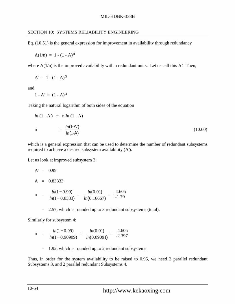
MIL-HDBK-338B


10-54

Eq. (10.51) is the general expression for improvement in availability through redundancy

A(1/n) = 1 - (1 - A)n

where A(1/n) is the improved availability with n redundant units. Let us call this A’. Then,

A’ = 1 - (1 - A)n

and

1 - A’ = (1 - A)n

Taking the natural logarithm of both sides of the equation

ln (1 - A’) = n ln (1 - A)

n = -A)(-A’)(

1

1

ln

ln(10.60)

which is a general expression that can be used to determine the number of redundant subsystemsrequired to achieve a desired subsystem availability (A’).

Let us look at improved subsystem 3:

A’ = 0.99

A = 0.83333

n =).(

).(833301

9901

−−

ln

ln =

).().(

166670

010

ln

ln =

-4.605-1.79

= 2.57, which is rounded up to 3 redundant subsystems (total).

Similarly for subsystem 4:

n =).(

).(9090901

9901

−−

ln

ln =

).().(

090910

010

ln

ln =

-4.605-2.397

= 1.92, which is rounded up to 2 redundant subsystems

Thus, in order for the system availability to be raised to 0.95, we need 3 parallel redundantSubsystems 3, and 2 parallel redundant Subsystems 4.



MIL-HDBK-338B


10-55

Note that we have not discussed the optimum allocation of failure and repair rates to achieve agiven availability; this will be done later in this section.

10.4.1.5 Model E - R&M Parameters Not Defined in Terms of Time

A very different situation in availability modeling is encountered when system “uptime” is notmeasured in hours of operation or any time parameter but rather in terms of number of roundsfired, miles traveled, actuations or cycles performed, etc. The reliability parameter is then nolonger expressed in terms of MTBF but rather in mean-rounds-between-failures (MRBF), mean-miles-between-failures (MMBF), mean-cycles-between-failures (MCBF), etc. The failure ratethen also is expressed in number of failures per round, per mile, or per cycle rather than numberof failures per operating hour.

For straightforward reliability calculations this poses no problem since the same reliabilityequations apply as in the time domain, except that the variable time, t, in hours is replaced by thevariable number of rounds, number of miles, etc. We may then calculate the reliability of suchsystems for one, ten, one hundred, or any number of rounds fired or miles traveled, as we wish.The maintainability calculations remain as before, since downtime will always be measured interms of time and the parameter of main interest remains the MTTR.

However, when it comes to availability, which usually combines two time parameters (i.e., theMTBF and the MTTR into a probability of the system being up at some time, t), a difficultproblem arises when the time, t, is replaced by rounds or miles, since the correlation betweentime and rounds or time and miles is quite variable.

An equation for the steady-state availability of machine guns is given in Reference [11]. This

equation is based on a mission profile that at discrete times, t1, t2, t3, etc., requires the firing of

N1, N2, N3, etc., bursts of rounds. When the gun fails during a firing, for example at time t, it

fires only f rounds instead of N3 rounds and must undergo repair during which time it is not

available to fire; for example, it fails to fire a required N4 rounds at t4, and a further N5 rounds at

t5 before becoming again available (see Figure 10.4-5). Its system availability, A, based on therounds not fired during repair may be expressed, for the described history, as:

A = (N1 + N2 + f)/(N1 + N2 + N3 + N4 + N5) (10.61)

Each sequence of rounds fired followed by rounds missed (not fired) constitutes a renewalprocess in terms of rounds fired, as shown in Figure 10.4-6, where the gun fails after firing xrounds, fails to fire γ(x) rounds in the burst of rounds during which it failed and also misses firingthe required bursts of rounds while in repair for an MTTR = M. Assume that the requirementsfor firing bursts of rounds arrives at random according to a Poisson process with rate r and theaverage number of rounds per burst is N, then the limiting availability of the gun may beexpressed as:

MIL-HDBK-338B


10-56

A = MRBF/(MRBF + N + γMN) (10.62)

where MRBF is the mean number of rounds between failure. The derivation of this formula,developed by R.E. Barlow, is contained in the Appendix of Reference [11]. To calculate A fromEq. (10.62) one must know the MRBF and MTTR of the gun, the average rounds N fired perburst, and the rate γ at which requirements for firing bursts of rounds arrive.

Repair Time

0 t t t t t

N N NN

N

1 2

3

4 5

1 2 3 4 6t

5

f

NU

MB

ER

OF

RO

UN

DS

FIR

ED

N3 - f

FIGURE 10.4-5: HYPOTHETICAL HISTORY OF MACHINE GUN USAGE



MIL-HDBK-338B


10-57

γ (x)

O N

N

N

f

x1

2

3

1

NUMBER OF ROUNDS FIRED

FIGURE 10.4-6: RENEWAL PROCESS IN TERMS OF ROUNDS FIRED

Similar availability equations can be developed for other types of weapons and also for vehicleswhere the renewal process is in terms of miles traveled. Other approaches to calculating theavailability of guns as well as vehicles are found in Reference [12] and are based on calculatingfrom historical field data the maintenance ratios and, via regression analysis, the maintenancetime ratios (called the “maintenance clock hour index”) that are in turn used in the conventionaltime based equation of inherent, achieved, and operational availability.

For example, consider a machine gun system in a tank on which historical data are available,showing that 0.014 corrective maintenance man-hours are expended per round fired and that peryear 4800 rounds are fired while the vehicle travels for 240 hr per yr. The maintenance ratio(MR) for the gun system is then computed as (Ref. [12], pp. 36-38).

MRGun =

MMHRound

• Number of Rounds Fired per AnnumVehicle Operating Hours per Annum

= 0.014 • (4800/240) = 0.28 (10.63)

The dimensions for 0.28 are gun system maintenance man-hours per vehicle operating hour.According to this example, the corrective maintenance time ratio, α (sometimes called themaintenance clock hour index, Ω), is, given by:

αGun = 0.628(0.28)0.952 = 0.187 (10.64)

MIL-HDBK-338B


10-58

The numbers 0.628 and 0.952 are the intercept and the regression coefficients, respectively,obtained by regression analysis as developed in Reference [12], p. 18, Table 1. The dimensionfor αGun is gun system downtime per vehicle operating hour. The inherent availability of the

gun system is then, according to the conventional time equation, Eq. (10.20).

Ai = (1 + αGun)-1 = (1.187)-1 = 0.842 (10.65)

This may be interpreted as the gun system being available for 84.2% of the vehicle operatingtime. Caution is required in using this approach for weapon availability calculations, since in thecase where the vehicle would have to be stationary and the gun would still fire rounds, MR and αwould become infinitely large and the inherent availability of the gun system would become zero.

10.4.2 Mission Reliability and Dependability Models

Although availability is a simple and appealing concept at first glance, it is a point concept, i.e., itrefers to the probability of a system being operable at a random point in time. However, theability of the system to continue to perform reliably for the duration of the desired operating(mission) period is often more significant. Operation over the desired period of time depends,then, on clearly defining system operating profiles. If the system has a number of operatingmodes, then the operating profile for each mode can be considered.

The term mission reliability has been used to denote the system reliability requirement for aparticular interval of time. Thus, if the system has a constant failure rate region so that itsreliability R can be expressed as:

R = exp (-λt) (10.66)

where:λ = failure rate = 1/MTBFt = time for mission

then mission reliability RM for a mission duration of T is expressed as:

RM = exp (-λT) (10.67)

This reliability assessment, however, is conditional upon the system being operable at thebeginning of its mission or its (point) availability.

In order to combine these two concepts, a simplified system effectiveness model may be usedwhere the system effectiveness may be construed simply as the product of the probabilities thatthe system is operationally ready and that it is mission reliable.



MIL-HDBK-338B


10-59

If A is the mean availability of a system at any point in time to when we want to use the system

and if RM is the system reliability during mission time T, then system effectiveness E, not

including performance, may be defined as:

E = ARM (10.68)

Thus, A is a weighting factor, and E represents an assessment of system ability to operate withoutfailure during a randomly chosen mission period.

One concept of dependability used by the Navy (Ref. [13]) takes into account the fact that forsome systems a failure which occurs during an operating period t1 may be acceptable if the

failure can be corrected in a time t2 and the system continues to complete its mission.

According to this concept, dependability may be represented by:

D = RM + (1 - RM)Mo (10.69)

where:D = system dependability - or the probability that the mission will be successfully

completed within the mission time t1, providing a downtime per failure not

exceeding a given time t2 will not adversely affect the overall mission

RM = mission reliability - or the probability that the system will operate without failure for

the mission time t1Mo = operational maintainability - or the probability that when a failure occurs, it will be

repaired in a time not exceeding the allowable downtime t2t2 = specified period of time within which the system must be returned to operation

For this model, the exponential approximation of the lognormal maintainability function is used,or

Mo =

1 - e-µt2 (10.70)

Then, the system effectiveness is:

E = AD = A

RM + (1 - RM) Mo (10.71)

MIL-HDBK-338B


10-60

In the case where no maintenance is allowed during the mission (t2 = 0 or Mo = 0), as in the

case of a missile, then this reduces to Eq. (10.68).

E = AD = ARM

This concept of dependability is compatible with the WSEIAC model and indeed can be takeninto account in the dependability state transition matrices.

Let us examine an airborne system with the following parameters and requirements:

λ = 0.028 failures/hr

µ = 1 repair/hr

Mission time (T) = 8 hours

ta = 30 minutes to repair a failure during a mission

Thus,

A = µ

µ + λ = 1

1 + 0.028 = .973 at the start of the mission

RM = e-λT = e-(0.028)(8) = 0.8 (mission reliability)

Mo = 1 - e-µta = 1 - e-(1)(0.5) = 0.4 (probability of repairing failure during

mission within

12

hour)

∴ E = A

RM + (1 - RM) Mo

= 0.973

0.8 + (1 - 0.8) (0.4)

= 0.973

0.8 + 0.08 = 0.86

10.4.3 Operational Readiness Models

Availability, defined as the uptime ratio, is not always a sufficient measure to describe the abilityof a system to be committed to a mission at any arbitrary time. In many practical militaryoperations, the concept of operational readiness serves this purpose better. We here define



MIL-HDBK-338B


10-61

operational readiness as the probability that a system is in an operable condition, i.e., ready to becommitted to perform a mission when demands for its use arise. The difference as well as thesimilarity between availability and operational readiness will become clear by comparing themodels developed subsequently with the availability models discussed in the preceding section.

In the development of operational readiness models, one has to consider the usage and themaintenance of the system, i.e., its operating, idle, and repair times. When a call arrives for thesystem to engage in a mission, the system at such time may be in a state of perfect repair andready to operate immediately. But it may also be in need of maintenance and not ready. Its statewhen called upon to operate depends on the preceding usage of the system, i.e., on its precedingmission, in what condition it returned from that mission, and how much time has elapsed since itcompleted the last mission. Many models can be developed for specific cases, and some arediscussed in the following paragraphs.

10.4.3.1 Model A - Based Upon Probability of Failure During Previous Mission andProbability of Repair Before Next Mission Demand

In this model, the assumption is made that if no failures needing repair occurred in the precedingmission, the system is immediately ready to be used again; and, if such failures did occur, thesystem will be ready for the next mission only if its maintenance time is shorter than the time bywhich the demand for its use arises. The operational readiness POR may then be expressed as:

POR = R(t) + Q(t) • P(tm < td) (10.72)

where:R(t) = probability of no failures in the preceding missionQ(t) = probability of one or more failures in the preceding missiont = mission duration

P(tm < td) = probability that if failures occur, the system maintenance time, tm, is shorter

than the time, td, at which the next demand or call for mission engagementarrives

The calculations of R(t) and Q(t) = 1 - R(t) are comparatively simple using standard reliabilityequations; however, all possible types of failures that need fixing upon return in order to restorein full the system reliability and combat capability must be considered, including any failures inredundant configurations.

As for P(tm < td), one needs to know the probability distributions of the system maintenance time

and of call arrivals. Denoting by f(tm) the probability density function of maintenance time and

by g(td), the probability density function of time to the arrival of the next call, counted from theinstant the system returned from the preceding mission in a state requiring repair, the probabilitythat the system will be restored to its full operational capability before the next call arrives is:

MIL-HDBK-338B


10-62

P(tm < td) =

t m

∞

∫ f(tm)

∫∞

=dd )dtg(t

md ttdtm (10.73)

The integral in the square brackets on the right side of the equation is the probability that the call

arrives at td after a variable time tm. When this is multiplied by the density function f(tm) of the

duration of maintenance times and integrated over all possible values of tm, we get P(tm< td).

Now assume that maintenance time tm and time to next call arrival td are exponentially

distributed, with M1 being the mean time to maintain the system and M2 the mean time to nextcall arrival. The probability density functions are thus:

f(tm) = exp(−tm/M1)[ ]/M1 (10.74)

f(td) = exp(−td/M2 )[ ]/M2 (10.75)

We then obtain

P(tm < td) =

0

∞

∫ M1-1 exp (-tm/M1) •

−−

∞

∫ d2d1

2 )dt/Mtexp(Mmt

dtm

=

0

∞

∫ (−M1−1)exp −(1/M1 +1/M2)tm[ ]dtm

= M2/(M1 + M2) (10.76)

In this exponential case, system operational readiness becomes

POR = R(t) + Q(t) •

M2 /(M1 + M2)[ ] (10.77)



MIL-HDBK-338B


10-63

As a numerical example let us look at a system with a probability of R = 0.8 of returning from amission of t = 1 hr duration without requiring repair and therefore had a probability of Q = 0.2

that it will require repair. If system mean maintenance time is M1 = 1 hr and the mean time to

next call arrival is M2 = 2 hr., the operational readiness of the system becomes

P = 0.8 + 0.2 (2/3) = 0.933

Comparing this result with the conventional steady-state availability concept and assuming that

the system has a mean maintenance time of M1 = 1 hr and a mean time to failure of M2 = 5 hr(roughly corresponding to the exponential case of R = 0.8 for a one-hour mission), we obtain asystem availability of:

A = M2/(M1 + M2) = 5/6 = 0.833

which is a result quite different from POR = 0.933.

10.4.3.2 Model B - Same As Model A Except Mission Duration Time, t is Probabilistic

The operational readiness model of Eq. (10.72) can be extended to the case when missionduration time t is not the same for each mission but is distributed with a density q(t). We thenget

POR =

R(t)q(t)dt

0

∞

∫ + P(tm < td)

Q(t)q(t)dt

0

∞

∫ (10.78)

Since the integrals in Eq. (10.78) are fixed numbers, we may write:

R =

R(t)q(t)dt

0

∞

∫ , and

Q =

Q(t)q(t)dt

0

∞

∫ (10.79)

and using the symbol P for P(tm < td), i.e., P = P(tm < td), Eq. (10.78) may be written in theform:

POR = R + QP (10.80)

In this equation R is the probability that the system returns without failures from the last mission;

MIL-HDBK-338B


10-64

Q = 1 - R is the probability that one or more failures developed in the last mission; and P is theprobability that the system will be repaired before the next call arrives if it developed failures.The mission times are variable here with density q(t).

10.4.3.3 Model C - Similar To Model A But Includes Checkout EquipmentDetectability

The operational readiness of the system at time ta is given by:

POR(ta) = R(tm) + kM(tr)[ ] • 1 − R(tm)[ ] (10.81)

where:

POR(ta) = probability of system being available for turnaround time, e.g., ta of 30 minutes,following completion of preceding mission or initial receipt of alert

R(tm) = probability that the system will survive the specified mission of duration tmwithout failure

tr = specified turnaround time, or maximum downtime for repair required of the

systemk = probability that if a system failure occurs it will be detected during the mission

or during system checkout following the mission

M(tr) = probability that a detected system failure can be repaired in time tr to restore thesystem to operational status

Thus, when mission reliability, mission duration, availability, and turnaround time are specifiedfor the system, the detectability-times-maintainability function for the system is constrained topass through or exceed the point given by:

kM(tr) ≥ POR(ta) - R(tm)

1 - R(tm)

Consider, for example, the following specified operational characteristics for a new weaponssystem:

Mission Reliability, R(tm) = 0.80 for tm of 8 hours

Operational Readiness POR(ta) = 0.95 for turnaround time, ta of 30 minutes, followingcompletion of preceding mission or initial receipt of alert.



MIL-HDBK-338B


10-65

From the requirements, the required detectability-maintainability product (kM) is derived asfollows:

kM(30) = POR(30) - R(8)

1 - R(8) = 0.95 - 0.8

1 - 0.8 = 0.75

Therefore, kM(30) = 0.75 is the joint probability, given that a system failure has occurred, thatthe failure will be detected (either during the mission or during post mission checkout) and willbe repaired within 30 minutes following completion of the mission.

Assume that k is to be 0.9, i.e., built-in test equipment is to be incorporated to detect at least 90%of the system failures and provide go/no-go failure indication.

Then, the maintainability requirement is:

M(30) = 0.75

k = 0.750.9 ≈ 0.83

which means that 83% of all system repair actions detected during the mission or during postmission checkout must be completed within 30 minutes.

Using the exponential approximation, maintainability as a function of repair time is expressed as

the probability of repair in time tr:

M(tr) = 1 - e −µtr = 1 - e −tr /Mct (10.82)

where:

Mct = MTTRµ = repair rate, 1/ Mct

tr = repair time for which M(t) is to be estimated

The required mean time to repair ( Mct ) is found from Eq. (10.82) by taking the natural log ofboth sides:

Mct = - tr

ln

1 - M(tr)

MIL-HDBK-338B


10-66

Substituting tr = 30 minutes, and M(tr), which we previously found to be 0.83,

Mct = - 30

ln (0.17) = -30

-1.77 ≈ 17 minutes

And from M(tmax) = 0.95 we find the maximum time for repair of 95% of detected system

failures (Mmaxct) as follows:

M(tmax) = 0.95 = 1 - e-Mmaxct/ M ct

Mmaxct= - M ct ln (1 - 0.95)

= - (17)(-3) = 51 minutes

Thus, these requirements could be established as design requirements in a system developmentspecification.

Detectability Factor, k = 0.90

Mean Time To Repair, M ct = 17 minutes

Maximum Time To Repair, Mmaxct= 51 minutes

10.4.3.4 Model D - For a Population of N Systems

Let N be the total population of systems, e.g., squadron of aircraft. The service facility itself shallbe considered as having k channels, each servicing systems at a mean rate µ. The analysis isbased on an assumed Poisson distribution of arrivals and on a mean service time which isassumed to be exponentially distributed. This service is performed on a first come, first servedbasis.

The basic equations (derived in Ref. [11]) are as follows:

pn =

N!(N − n)!

ρk

k!

ρk

n−kpo when n > k (10.83)

pn =N!

(N - n)! ρn

n! po when n ≤ k

(10.84)



MIL-HDBK-338B


10-67

po =

1knkk

0n

nk

1kn kk!n)!(N

N!

n!n)!(N

N!−−

=+=

−

+−

∑∑ (10.85)

ρ =λµ =

Mean arrival rate (failure)Mean service rate (10.86)

where:pi = probability of i units awaiting service

k = number of repair channels or facilitiesN = total number of systems

POR = N - n

N (10.87)

where: POR = probability that a system is neither awaiting nor undergoing service.

n = average number of systems either awaiting or undergoing service at

a given time and is defined by:

n = n =0

N

∑ npn (10.88)

The specific procedure, which will be illustrated by an example, is as follows:

Step 1: Use Eq. (10.85) to solve for po

Step 2: Use po from Step 1 to help derive pn for all values of n ≤ k by use of

Eq. (10.84)

Step 3: Use po from Step 1 to help derive pn for all values of n > k by use of Eq.

(10.83)

Step 4: For all values of n, from 0 through N, sum the terms npn derived from Steps 1

through 3. This, per Eq. (10.88) gives n , the average number of systems not

ready

Step 5: Use Step 4 results and Eq. (10.87) to obtain the operational readiness probability,POR

MIL-HDBK-338B


10-68

Example 12: POR of Interceptor Squadron

An interceptor squadron contains fifteen planes (N = 15) and has available four flight line repairchannels (k = 4). Each plane averages 50 operating hours per month out of 24 times 30, or 720total available hours. Because of five-day, two-shift maintenance each failure requires anaverage of five clock hours (MTTR) to repair. The plane MTBF is 3.47 operating hours betweenfailures. What is the operational readiness probability for this squadron?

We first compute the utilization factor ρ.

r =

1ρ

• Operating hours per plane per month

Total hours per month

=))(.(

))((720473

505 =

2500

250 = 0.1

Step 1: Use Equation (10.85) to obtain po

po =

1knkN

km

nN

1kn k

r

k!

r

n)!(N

N!

n!

r

n)!(N

N!−−

=+=

−

+− ∑∑

po =

14n415

4m

n4

0m 4

(0.1)

4!

(0.1)

n)!(15

15!

n!

(0.1)

n)!(15

15!−−

==

−

+− ∑∑



MIL-HDBK-338B


10-69

The calculated results are shown in the following table:

n Term (1) Term (2)

0 1.0 - -1 1.5 - -2 1.05 - -3 0.455 - -4 0.1365 0.034125 - - 0.03756 - - 0.037537 - - 0.03378 - - 0.01279 - - 0.018910 - - 0.011311 - - 0.005612 - - 0.002213 - - 0.000614 - - 0.0001315 - - 0.00000

Sum 4.1415 0.19428

po = (4.1415 + 0.19428)-1 = (4.3358)-1 = 0.2306

Step 2: Use Equation (10.84) and obtain pn for n = 1 through 4.

Pn = N!

(N - n)! ρn

n! po

Thus,

p1 = 15!

(15 - 1)! (0.1)1

1! (0.23) = 0.3450

p2 = 15!13!

(0.1)2

2! (0.23) = 0.2415

p3 = 15!12!

(0.1)3

3! (0.23) = 0.10465

p4 = 15!11!

(0.1)4

4! (0.23) = 0.0313

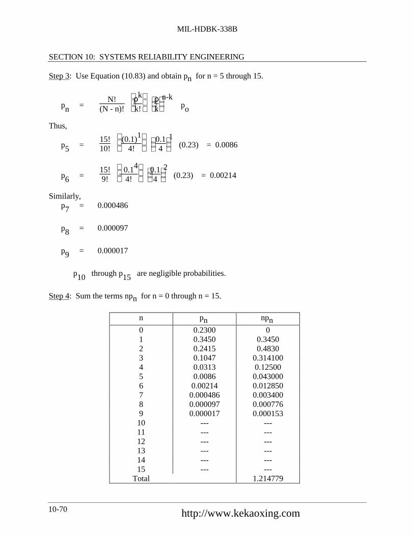
MIL-HDBK-338B


10-70

Step 3: Use Equation (10.83) and obtain pn for n = 5 through 15.

pn = N!

(N - n)!

ρk

k!

ρ

k

n-k po

Thus,

p5 = 15!10!

(0.1)1

4!

0.14

1 (0.23) = 0.0086

p6 = 15!9!

0.14

4!

0.1

4

2 (0.23) = 0.00214

Similarly,p7 = 0.000486

p8 = 0.000097

p9 = 0.000017

p10 through p15 are negligible probabilities.

Step 4: Sum the terms npn for n = 0 through n = 15.

n pn npn

0 0.2300 01 0.3450 0.34502 0.2415 0.48303 0.1047 0.3141004 0.0313 0.125005 0.0086 0.0430006 0.00214 0.0128507 0.000486 0.0034008 0.000097 0.0007769 0.000017 0.00015310 --- ---11 --- ---12 --- ---13 --- ---14 --- ---15 --- ---

Total 1.214779



MIL-HDBK-338B


10-71

Therefore from Equation (10.88):

n = n =0

N

∑ npn

= 1.215 planes which are not ready on the average

Step 5: Using Step 4 results and Equation (5.87), we obtain POR, the operational readinessprobability

POR = N - n

N = 15 - 1.215

15 = 13.785

15 = 0.919

As can be seen, the calculations are rather laborious and best done by a computer. Figures 10.4-7and 10.4-8 (from Ref. [10]) are a series of curves for N = 15 and N = 20 with k values rangingfrom 1 to 10 and 1 to 20, respectively. Note that 0.919 checks out the r = 0.1, k = 4 point onFigure 10.4-7.

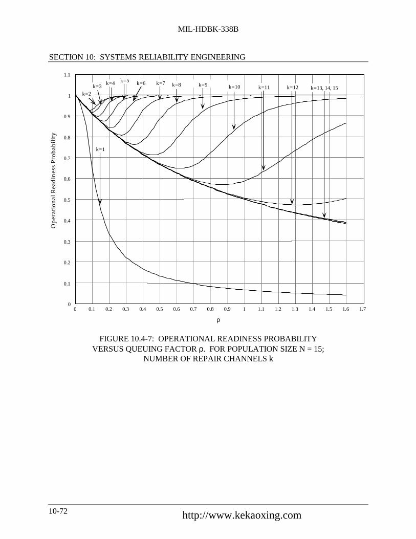
MIL-HDBK-338B


10-72

0

0.1

0.2

0.3

0.4

0.5

0.6

0.7

0.8

0.9

1

1.1

0 0.1 0.2 0.3 0.4 0.5 0.6 0.7 0.8 0.9 1 1.1 1.2 1.3 1.4 1.5 1.6 1.7

Op

erat

iona

l Rea

din

ess

Pro

babi

lity

ρ

k=1

k=13, 14, 15k=12k=11k=10k=2

k=3 k=4 k=5 k=6 k=7 k=8 k=9

FIGURE 10.4-7: OPERATIONAL READINESS PROBABILITYVERSUS QUEUING FACTOR ρ. FOR POPULATION SIZE N = 15;

NUMBER OF REPAIR CHANNELS k



MIL-HDBK-338B


10-73

.

k=9

0

0.1

0.2

0.3

0.4

0.5

0.6

0.7

0.8

0.9

1

1.1

0 0.1 0.2 0.3 0.4 0.5 0.6 0.7 0.8 0.9 1 1.1 1.2 1.3 1.4 1.5 1.6 1.7

Ope

rati

onal

Rea

din

ess

Prob

abili

ty

k=1

k=2k=3 k=4 k=5 k=6 k=7 k=8 k=10 k=11 k=12 k=13,14,15

ρ

FIGURE 10.4-8: OPERATIONAL READINESS PROBABILITYVERSUS QUEUING FACTOR ρ. FOR POPULATION SIZE N = 20;

NUMBER OF REPAIR CHANNELS k

10.5 Complex Models

In summing up the discussion of models, it should be recognized that there may be othermeasures of system R&M parameters or system effectiveness than those previously discussed.For example, in cases such as manned aircraft models it might be meaningful to combineoperational readiness and equipment availability into one index, or we may wish to combinedetection probability and availability for a ground radar system to be an index of the probabilitythat a raid launched at any random time will be detected. The important point in selecting anindex of system reliability effectiveness is recognizing that it is equivalent to a correct statementof the problem.

When selecting an index of effectiveness we should keep in mind some characteristics withoutwhich the index would be of little value. Probably the most important characteristic is that theindex be expressed quantitatively. We should be able to reduce it to a number such thatcomparisons between alternative designs can be made. Furthermore, the index we choose must

MIL-HDBK-338B


10-74

have a basis in physical reality. Thus it should be descriptive of the real problem, not exaggeratedor oversimplified. Yet at the same time the index should be simple enough to allow formathematical manipulation to permit evaluating alternatives.

In complex system effectiveness mathematical models, an attempt is made to relate the impact ofsystem reliability, maintainability, and performance to the mission profiles, scenario, use, andlogistic support. Only in simple situations can a meaningful single model be developed that willrelate all these parameters and yield a single quantitative measure of system effectiveness.Numerous complex computerized models exist and, as a matter of fact, every major company inthe aerospace business has developed a multitude of such models.

10.6 Trade-off Techniques

10.6.1 General

A trade-off is a rational selection among alternatives in order to optimize some system parameterthat is a function of two or more variables which are being compared (traded off). Examples ofsystem trade-offs involve performance, reliability, maintainability, cost, schedule, and risk. Atrade-off may be quantitative or qualitative. Insofar as possible, it is desirable that trade-offs bebased on quantifiable, analytic, or empirical relationships. Where this is not possible, then semi-quantitative methods using ordinal rankings or weighting factors are often used.

The methodology for structuring and performing trade-off analyses is part of the systemengineering process described in Section 4. The basic steps, summarized here are:

(1) Define the trade-off problem and establish the trade-off criteria and constraints

(2) Synthesize alternative design configurations

(3) Analyze these alternative configurations

(4) Evaluate the results of the analyses with respect to the criteria, eliminating those whichviolate constraint boundaries

(5) Select the alternative which best meets criteria and constraint boundaries or iterate thedesign alternatives, repeating Steps 2 through 5 to obtain improved solutions



MIL-HDBK-338B


10-75

System effectiveness and cost effectiveness models provide the best tools for performing trade-off studies on the system level. Through the computerized models, any changes in any of themultitude of reliability, maintainability, performance, mission profile, logistic support, and otherparameters can be immediately evaluated as to their effect on the effectiveness and total cost of asystem. Thus, cost effectiveness modeling and evaluation, besides being used for selecting aspecific system design approach from among several competing alternatives, is a very powerfultool for performing parametric sensitivity studies and trade-offs down to component level whenoptimizing designs to provide the most effective system for a given budgetary and life cycle costconstraint or the least costly system for a desired effectiveness level.

At times, however, especially in the case of the more simple systems, trade-offs may be limitedto achieving a required system availability while meeting the specified reliability andmaintainability requirements. Comparatively simple trade-off techniques can then be used asshown in the following paragraphs.

10.6.2 Reliability - Availability - Maintainability Trade-offs

The reliability-maintainability-availability relationship provides a measure of systemeffectiveness within which considerable trade-off potential usually exists, e.g., betweenreliability, maintainability, and logistic support factors. This potential should be re-evaluated ateach successive stage of system development to optimize the balance between reliability,maintainability, and other system effectiveness parameters with respect to technical risks, lifecycle cost, acquisition schedule, and operating and maintenance requirements. The latter becomeincreasingly more important as complexity of system design increases, dictating the need forintegration of system monitoring and checkout provisions in the basic design.

As stated earlier in this section and in Section 2, reliability and maintainability jointly determinethe inherent availability of a system. Thus, when an availability requirement is specified, there isa distinct possibility of trading-off between reliability and maintainability, since in the steadystate availability depends only on the ratio or ratios of MTTR/MTBF which was previouslyreferred to as maintenance time ratio (MTR), α , i.e.,

α = MTTR/MTBF = λ/µ (10.88)

so that the inherent availability equation assumed the form

Ai = 1/(1 + α) (10.89)

As an example, consider systems I and II with

MTTRI = 0.1 hr.

MTBFI = 2 hr.

MIL-HDBK-338B


10-76

MTTRII = 10 hr.

MTBFII = 200 hr.

Then the steady state availability is

AI = 1/

1 + (0.1/2) = 0.952

AII = 1/

1 + (10/200) = 0.952

Both systems have the same availability, but they are not equally desirable. A 10-hr MTTRmight be too long for some systems, whereas a 2-hr MTBF might be too short for some systems.

Even though reliability and maintainability individually can be increased or decreased incombinations giving the same system availability, care must be taken to insure that reliabilitydoes not fall below its specified minimum or that individually acceptable values of reliability andmaintainability are not combined to produce an unacceptable level of system availability.

A generalized plot of Eq. (10.88) is given in Figure 10.6-1. A plot of A vs. λ/µ, is given inFigure 10.6-2. These equations and graphs show that in order to optimize availability it isdesirable to make the ratio of MTBF/MTTR as high as possible.

Since increasing MTBF and decreasing MTTR is desirable, the equation for availability can beplotted in terms of MTBF and 1/MTTR (or µ) as shown in Figure 10.6-3. Each of the curvesrepresenting the same availability in Figure 10.6-3 just as each of the lines in Figure 10.6-1, iscalled isoavailability contours; corresponding values of MTBF and MTTR give the same value ofA, all other things being equal. Availability nomographs useful for reliability and maintainabilitytrade-offs are given in Reference [13]. Figure 10.6-4 is an example of an availability nomograph.



MIL-HDBK-338B


10-77

1 2 3 4 5 6 7 8 9 10

1

2

3

4

5

6

7

8

9

10

00

A=1 A=0.9

A=0.75

A=0.5

A=0.25

A=0.1

A=0

MTBF

MTTR

(A) AVAILABILITY AS A FUNCTION OF MTBF AND MTTR

1 2 3 4 5 6 7 8 9 10

1

2

3

4

5

6

7

8

9

10

00

A=0 A=0.1

A=0.25

A=0.5

A=0.75

A=0.9

A=1

λ

µ

(B) AVAILABILITY AS A FUNCTION OF λ AND µ

FIGURE 10.6-1: RELIABILITY - MAINTAINABILITY -AVAILABILITY RELATIONSHIPS

MIL-HDBK-338B


10-78

1 2 3 4 5 6 7 8 9 100 11 120

0.1

0.2

0.3

0.4

0.5

0.6

0.7

0.8

0.9

1.0

A

λ/µ

FIGURE 10.6-2: AVAILABILITY AS A FUNCTION OF λ/µ

0 3 6 9 12 15

3

6

9

12

15

MTBF

1/MTTR, µ

A=0.99

0.98

0.960.950.90

0.800.750.50

FIGURE 10.6-3: AVAILABILITY AS A FUNCTION OF MTBF AND 1/MTTR



MIL-HDBK-338B


10-79

10.0

8.0

6.0

5.0

4.0

3.0

2.0

0.1

1.0

100

50

1000

500

10000

5000

10

0.8

0.6

0.5

0.4

0.3

0.2

0.90

0.92

0.94

0.95

0.96

0.97

0.98

0.9990

0.9992

0.9994

0.9995

0.9996

0.9997

0.9998

0.99990

0.99992

0.99994

0.99996

0.99995

0.99997

0.999985

0.999990

1.5

3000

0.99998

MTTR (hr)

MTBF ( hr)

Ai

0.985

FIGURE 10.6-4: AVAILABILITY NOMOGRAPH

MIL-HDBK-338B


10-80

There are obvious practical limits which must be considered in trade-off optimization. These arecalled constraints, and all purposeful optimization must be bounded by constraints into feasibleregions. For example, there are practical limits as to how high a value for MTBF can beachieved or how low MTTR can be made. In the one case, the reliability of system componentsor the required redundancy might be so high that the desired reliability could not be realisticallyachieved within the state-of-the-art or would be so expensive as to violate cost constraints.Similarly, MTTRs close to zero would require extreme maintainability design features, such ascompletely built-in test features or automatic test and checkout to allow fault isolation to eachindividual replaceable module, with perhaps automatic switchover from a failed item to astandby item. This also could easily violate state-of-the-art or cost constraints.

It follows, then, that trade-offs not only involve relationships among system parameters andvariables but also that they are bounded by both technical and economic constraints. In a sense,all trade-offs are economic ones, requiring cost-benefit analysis (not necessarily in terms ofdollar costs but rather in terms of the availability and consumption of resources, of which dollarsare often the most convenient measure). Resource constraints may also include manpower andskill levels, schedule or time availability, and the technical state-of-the-art capability. Latersections of this chapter deal with the cost problem.

There are two general classes of trade-offs. In the first, the contributing system variables aretraded-off against one another without increasing the value of the higher level system parameter;for example, trading-off reliability and maintainability along an isoavailability contour (nochange in availability). This might be done for reasons of standardization or safety or foroperational reasons such as the level at which the system and its equipments will be maintained.The other class of trade-off is one in which the system variables are varied in order to obtain thehighest value of the related system parameters within cost or other constraints. For example,reliability and maintainability might be traded-off in order to achieve a higher availability. Thiscould result in moving from one isoavailability curve to another in Figure 10.6-3, perhaps alongan isocline (a line connecting equal slopes).

An example of a reliability - availability - maintainability (RAM) trade-off is given in thefollowing paragraphs. The design problem is as follows: A requirement exists to design a radarreceiver which will meet an inherent availability of 0.99, a minimum MTBF of 200 hours, and anMTTR not to exceed 4 hours. The current design is predicted to have an availability of 0.97, anMTBF of 150 hours, and an MTTR of 4.64 hours.

Using Eq. (10.88) the area within which the allowable trade-off may be made is shown by thecross-hatched portion of Figure 10.6-5. As indicated in the previous paragraph, there are twoapproaches which can be used for trade-off. One is to fix the availability at 0.990. This meansthat any combination of MTBF and MTTR between the two allowable end points on the 0.990isoavailability line may be chosen. These lie between an MTBF of 200 hours with an MTTR of2 hours and an MTBF of 400 hours with an MTTR of 4 hours. The other approach is to allowavailability to be larger than 0.990 and thus allow any combination of MTBF and MTTR withinthe feasible region.



MIL-HDBK-338B


10-81

It is clearly seen that without any additional constraints the designer has a limitless number ofcombinations from which to choose. Assume that the following four alternative designconfigurations have been selected for trade-off as shown in Table 10.6-1.

Design Configuration Nos. 1, 2, and 3 all have the required availability of 0.990. DesignConfiguration No. 1 emphasizes the maintainability aspects in design, while DesignConfiguration No. 3 stresses reliability improvement. Design Configuration No. 2 is betweenNos. 1 and 3 for the same availability. Design Configuration No. 4 is a combination of Nos. 1and 2 and yields a higher availability.

Since all of these alternatives are within the feasible region shown in Figure 10.6-5 some othercriterion must be used for selection of the desired configuration. In this case, we will use theleast cost alternative or the one showing the greatest life cycle cost savings over the presentconfiguration as the basis for trade-off decision. An example cost comparison of the differentalternatives is shown in Table 10.6-2 (such costs would be estimated using various cost andeconomic models).

The cost table shows that Configuration No. 2 is the lowest cost alternative among those withequal availabilities. It also shows that Configuration No. 4, with a higher acquisition cost, has asignificantly better 10-year life cycle support cost and lowest overall cost, as well as a higheravailability. Thus Configuration No. 4 is the optimum trade-off, containing both improvedreliability and maintainability features.

The trade-off example previously shown was a relatively simple example for the case of a singleequipment. Let us now look at a more complex example. Figure 10.6-6 (a repeat of Figure 10.4-4) represents a serial system consisting of five statistically independent subsystems, each with theindicated MTBFi and MTTRi . We found by the use of Eq. (10.27) that the steady state

availability was:

A = i=1

5

∏ Ai = 0.73534

MIL-HDBK-338B


10-82

.

2018161412108642

MEAN-TIME-TO-REPAIR (MTTR), HR

0

100

200

300

400

500

600

700

800

900

1000

ME

AN

-TIM

E-B

ET

WE

EN

-FA

ILU

RE

(MT

BF)

, HR

A = .99

A = .98

A = .96

A = .92

TRADE-OFF AREA WITHIN SPECIFICATION

OUT OF SPECIFICATION

REQUIREMENTA = 99%MTBF = 200 HR MINMTTR = 4 HR MAX

A = .97

FIGURE 10.6-5: RELIABILITY-MAINTAINABILITY TRADE-OFFS



MIL-HDBK-338B


10-83

TABLE 10.6-1: ALTERNATIVE DESIGN TRADE-OFF CONFIGURATIONS

Design Configuration A MTBF, hr MTTR, hr1. R - derating of military standard parts 0.990 200 2.0

M - modularization and automatic testing2. R - design includes high reliability

parts/components0.990 300 3.0

M - limited modularization and semi-automatic testing

3. R - design includes partial redundancy 0.990 350 3.5M - manual testing and limited

modularization4. R - design includes high reliability

parts/components0.993 300 2.0

M - modularization and automatic testing

TABLE 10.6-2: COST COMPARISON OF ALTERNATIVEDESIGN CONFIGURATIONS

ITEM EXISTING 1 2 3 4Acquisition (Thousands of Dollars)

RDT&E 300 325 319 322 330Production 4,500 4,534 4,525 4,530 4,542

Total 4,800 4,859 4,844 4,852 4,87210-Year Support Costs(Thousands of Dollars)

Spares 210 151 105 90 105Repair 1,297 346 382 405 346Training and Manuals 20 14 16 8 14Provisioning & Handling 475 525 503 505 503

Total 2,002 1,036 1,006 1,018 968LIFE CYCLE COST 6,802 5,895 5,850 5,870 5,840

MIL-HDBK-338B


10-84

MTBF = 200 λ = 0.005MTTR = 1 µ = 1

SUBSYSTEM 2

MTBF = 25 λ = 0.040MTTR = 5 µ = 0.2

SUBSYSTEM 3

MTBF = 50 λ = 0.020MTTR = 5 µ = 0.1

SUBSYSTEM 4

MTBF = 400 λ = 0.0025MTTR = 2 µ = 0.5

SUBSYSTEM 5

MTBF = 100 λ = 0.010MTTR = 2 µ = 0.5

SUBSYSTEM 1

FIGURE 10.6-6: BLOCK DIAGRAM OF A SERIES SYSTEM

By inspection of the maintenance time ratios (MTRs) of each of the subsystems we note thatSubsystems 3 and 4 have the lowest MTRs, given by:

MTTRiMTBFi

= 525 = 0.2

for Subsystem 3 and 5/50 = 0.1 for Subsystem 4. These are, therefore, the “culprits” in limitingsystem availability to 0.73534, which may be unacceptable for the mission at hand. If because ofthe state-of-the-art limitations we are unable to apply any of the design techniques detailed inSection 7 to reduce MTBF, then our first recourse is to add a parallel redundant subsystem toSubsystem 3, the weakest link in the series chain.

We shall consider two cases: (1) the case where no repair of a failed redundant unit is possibleuntil both redundant subsystems fail and the system stops operating; or (2) repair is possible by asingle repair crew while the system is operating.

For case (1) where both units must fail before repair is initiated and a single crew repairs bothfailed units in sequence:



MIL-HDBK-338B


10-85

A(1/2) =

µ+

λ∑

λ∑

=

=n

n

n

n

n

1

1

2

1

2

1 =

1λ +

12λ

1λ +

12λ +

2µ

(from Equation 10.56)

=

10.04

+1

2(0.04)1

0.04+ 1

2(0.04)+ 2

0.2

= 37.547.5 = 0.789

This is a lower availability than the nonredundant case!

ASystem =

1

1+ MTTRSeriesMTBFSeries

= 1

1 + .02 = 0.833 (based on Equation 10.18)

For case (1), where both units must fail before repair is initiated and two repair crewssimultaneously repair both failed units:

A(1/2) =

n=1

2

∑ 1nλ

n=1

2

∑ 1nλ

+ 1µ

=

10.04

+1

2(0.04)1

0.04+ 1

2(0.04)+ 1

0.2

= 37.542.5 = 0.882

which is a slight improvement over the nonredundant case.

For case (2), where a single repair crew initiates repair action on a redundant subsystem as soonas it fails

A =

µ2 + 2µλ

µ2 + 2µλ + λ2 (from Table 10.4-1)

= (0.2)2 + 2(0.2)(0.04)

(0.2)2 + 2(0.2)(0.04) + (0.04)2

=

0.04 + 0.0160.04 + 0.016 + 0.0016

=

0.0560.0576

= 0.972

as compared to 0.833 where no redundancy was used.

MIL-HDBK-338B


10-86

This corresponds to an increased system availability of

A = 0.73534

0.9720.833

= 0.86

If this new value is still not acceptable redundancy might have to be applied to Subsystem 4. Forexample, let us use a 2-unit standby configuration for Subsystem 4 with multiple repairs; then(from Table 10.4-1), the steady state availability would be:

A =

2µ2 + 2µλ2µ2 + 2µλ + λ2 =

2(0.2)2 + 2(0.2)(0.02)

2(0.2)2 + 2(0.2)(0.02) + (0.02)2

=

0.08 + 0.0080.08 + 0.008 + 0.0004

= 0.0880.0884 = 0.995

Thus, the new system availability would be:

A = (0.86)

0.9950.909

= 0.94

where 0.909 was the original availability of Subsystem 4.

Note, however, that to achieve these gains in availability, repair of failed redundant units must bepossible while the system is operating.

Before leaving the subject of trade-offs at the system availability level, it should be pointed outthat design trade-off methodologies can also be used at lower levels of the system hierarchy toincrease MTBF and reduce MTTR. These are discussed in Section 7.

10.7 Allocation of Availability, Failure and Repair Rates

The previous sections discussed how availability can be calculated for various systemconfigurations, e.g., series, parallel, etc., and how R&M can be traded off to achieve a givenavailability. This section discusses methods for allocating availability (and, where appropriate,failure and repair rates) among the system units to achieve a given system availability.

The reader should keep in mind that we are concerned with systems that are maintained uponfailure. For the case of non-maintained systems, e.g., missiles, satellites, etc., the methodspresented in Chapter 3 are appropriate for system reliability design, prediction, and allocation.

During the initial design phase of a program, detailed information is not usually availableregarding the particular equipments to be employed with the system. For example, we may knowthat a transmitter with certain power requirements may be designed, but we do not usually know



MIL-HDBK-338B


10-87

if it is less expensive to design for a low failure rate or a high repair rate. Unless the experienceof similar, previously designed transmitters can guide our decisions, estimation of the best set ofalternatives is necessary. Having developed a system configuration, a range of values ofequipment failure rates and repair rates that would satisfy the system availability requirement canbe initially specified. The state-of-the-art limits for these equipments may not be known or theexpenditures required for improvement, but we can specify their ratio, which would allowconsiderable freedom through the design process.

10.7.1 Availability Failure Rate and Repair Rate Allocation for Series Systems

Several cases can be considered:

(1) A single repairman must repair any one of n identical, statistically independentsubsystems in series. The ratio of failure rate to repair rate is such that there is a strongpossibility that a second subsystem will fail while the first one is being repaired.

(2) Same as (1) except a repairman is assigned to each subsystem and can only work onthat particular subsystem.

(3) Same as (1) except some intermediate number of repairmen, r, less than the number ofsubsystems is assigned. Any repairman can work on any system.

(4) Repeat cases (1)-(3) with nonidentical subsystems.

10.7.1.1 Case (1)

The steady state availability in Case (1) is from Reference [25]:

As =

(µ/λ)n

n!i =0

n

∑ (µ/λ)i

i!

(10.90)

where:µ = subsystem repair rateλ = subsystem failure raten = number of subsystems in seriesµ/λ = “operability ratio” as opposed to λ/µ (the utilization factor)

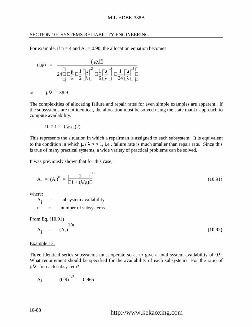
MIL-HDBK-338B


10-88

For example, if n = 4 and As = 0.90, the allocation equation becomes

0.90 = ( )

+

+

++

432

4

24

1

6

1

2

1124

or µ/λ = 38.9

The complexities of allocating failure and repair rates for even simple examples are apparent. Ifthe subsystems are not identical, the allocation must be solved using the state matrix approach tocompute availability.

10.7.1.2 Case (2)

This represents the situation in which a repairman is assigned to each subsystem. It is equivalentto the condition in which µ / λ > > 1, i.e., failure rate is much smaller than repair rate. Since thisis true of many practical systems, a wide variety of practical problems can be solved.

It was previously shown that for this case,

As = (Ai)n =

11 + (λ/µ)

n (10.91)

where:Ai = subsystem availability

n = number of subsystems

From Eq. (10.91)

Ai = (As)1/n

(10.92)

Example 13:

Three identical series subsystems must operate so as to give a total system availability of 0.9.What requirement should be specified for the availability of each subsystem? For the ratio ofµ/λ for each subsystem?

Ai = (0.9)1/3 = 0.965



MIL-HDBK-338B


10-89

0.965 = 1

1 + λ/µ

λ/µ =

10.965

- 1 = 0.036

Example 14:

A system consists of three identical, independent subsystems connected in series. Theavailability requirement is 0.99, and the repair rate is limited to 0.3 per hr. What is the minimumfailure rate which must be allocated to each subsystem to satisfy the system requirement? Arepairman is assigned exclusively to each subsystem.

If for Case (2) the series equipments are not identical the relationship

As = i=1

n

∏ Ai (10.93)

can be used to derive the individual subsystem availabilities.

Procedure Example

(1) State the system availability requirement. As = 0.99

(2) Compute the availability of each subsystem

by Ai = (As)1/n Ai = (0.99)13

= 0.99666

(3) For each subsystem compute the ratio λ / µby:

λ / µ =

10.99666

- 1

λµ

=

1Ai

- 1= 0.00336

(4) Compute λ from the previous equation withµ = 0.3 per hr. The final answer is roundedoff to 2 significant figures to avoid implyingtoo much accuracy.

λ = 0.00336 x (0.3 per hr)= 1.0 per 1000 hr

MIL-HDBK-338B


10-90

Example 15: (using Eq. (10.93))

Three subsystems must operate to give a total system availability of 0.9. Subsystem 1 has anavailability of 0.99. What should be specified for the availability of each of the other twosubsystems if: (1) they are equally important, or (2) Subsystem 3 should have twice theavailability of Subsystem 2 (this is interpreted as Subsystem 3 having one-half the unavailabilityof Subsystem 2).

(1) As = 0.99 A2A3

A2 = A3

0.9 = 0.99(2)A2

A2 = 0.91

A2 = A3 = 0.954

(2) (1 - A2) = 2 (1 - A3)

1 - A2 = 2 - 2A3

A3 = A2 + 1

2

0.9 = 0.99 A2A3 = 0.99 A2

+

2

1A2 = 0.99 A2

+2

A

2

2

2A

2

2

0.99

0.9 = A 2

2 + A2

A 22 + A2 - 1.82 = 0

A2 = 0.94

A3 = 0.94 + 1

2 = 0.97



MIL-HDBK-338B


10-91

The failure and repair rate allocations for A2 and A3 would be

λ2/µ2 =

1A2

- 1 = 1

0.94 - 1 = 0.064

λ3/µ3 =

1A2

- 1 =

10.97

- 1 = 0.03

The previous example can be expanded to use weighting factors to derive the required subsystemavailabilities. The choice of weighting factor would depend upon the system being analyzed andthe significant parameters affecting availability. Some examples of weighting factors might berelative cost or equivalent complexity of the subsystem. The latter, for example, should correlatesomewhat with increasing failure and repair rates. Let us examine an example of an allocationusing equivalent complexity.

Example 16:

A ground surveillance series system consists of a radar, a data processor, and display subsystem.A system availability of 0.995 is required. Based upon past experience and engineering analysis,it is estimated that the complexity of each subsystem is as follows:

Display Subsystem § 1000 component partsRadar Subsystem § 2500 component partsData Processor Subsystem § 5500 component parts

What availability requirement should be specified for each of the subsystems to meet the systemrequirement?

The weight assigned to each subsystem is given by:

Wi = Number of parts for subsystem iTotal number of parts in system

W1(Display) = 1000

1000 + 2500 + 5500 = 0.11

W2 (Radar) = 2500

1000 + 2500 + 5500 = 0.28

W3 (Data Processor) = 5500

1000 + 2500 + 5500 = 0.61

MIL-HDBK-338B


10-92

If the system availability requirement is 0.995, then 1 - 0.995 = 0.005 is the unavailability of thesystem. Using the weights previously derived to apportion the system unavailability to each ofthe subsystems, we get:

Display = (0.11)(0.005) = 0.00055Radar = (0.28)(0.005) = 0.00140Data Processor = (0.61)(0.005) = 0.00305

SYSTEM UNAVAILABILITY = 0.005

Thus, the required availabilities for each subsystem would be

A1 (Display) = 1 - 0.00055 = 0.99945

A2 (Radar) = 1 - 0.0014 = 0.9986

A3 (Data Processor) = 1 - 0.00305 = 0.99695

Verifying that the system requirement will be met

As = (0.99945)(0.9986)(0.99695) = 0.995

Also, as was previously shown, failure and repair rate allocation can be derived:

λ1/µ1 =

1A1

- 1 =

10.99945

- 1 = 5.5 • 10-4

λ2/µ2 =

1A2

- 1 =

10.9986

- 1 = 1.4 • 10-3

λ3/µ3 =

1A3

- 1 =

10.99695

- 1 = 3.0 • 10-3

Another slight variation of Case (2) (Section 10.7.1.2) is a series system with nonidenticalsubsystems, in which each subsystem's

λi/µi < 0.1

The availability of such a system with subsystems whose failures and repair are statisticallyindependent is:

As =

1

1+i=1

n

∑ αi

(10.94)



MIL-HDBK-338B


10-93

where:

αi = λi/µi with all αi < 0.1n = number of subsystems in seriesα (system) = α1 + α2 + ... + αn (10.95)

To design such a system, one merely allocates the subsystem αi’s according to some weightingscheme. For example, there may be a requirement to design a new system with higheravailability which is similar in design to the old system, where the relative weighting factors arethe same for each new subsystem.

Wi = αi (new)

αi (old) (10.96)

Example 17:

A system consisting of two statistically independent subsystems has an availability of 0.90.Subsystem 1 has an availability of 0.97, and subsystem 2 has an availability of 0.93. A newsystem, similar in design to this one, must meet a required 0.95 availability. What are the newsubsystem availabilities and ratios of failure-to-repair rate?

Since the allocated ratios are known, additional trade-off studies can be performed to optimize

λi and µi for each subsystem.

10.7.2 Failure and Repair Rate Allocations For Parallel Redundant Systems

A system comprising several stages of redundant subsystems whose λ/µ ratio is less than 0.1 can

be treated as if the stages were statistically independent. The system steady-state availability Asis:

As = A1 • A2 • A3 • ... • An

where:

Ai = the availability of State I

The procedure for allocating the failure and repair rates and the availability is as follows.

MIL-HDBK-338B


10-94

Procedure Example

(1) State the availability requirement As = 0.95

As of the new system

(2) Compute the sum αs of the (Remember αi = λi/µi =

1Ai

- 1)

α = ratios for the old system αs(old) = 0.0309 + 0.0753 = 0.01062

αs(old) = α1 + α2

(3) Compute the relative weights Wi by Eq. (10.96)

W1 =

0.03090.1062

= 0.291

W2 =

0.07530.1062

= 0.709

(4) Compute an overall As for the new system by:

αs’ (new) = 1

As’ - 1 αs’ = 1

0.95 - 1 = 0.0526

(5) Compute the allocated αi’ for each subsystemof the new design by:

α1 = (0.291) (0.0526) = 0.0153

αi’ = Wi αs’ α2’ = (0.709) (0.0526) = 0.0373

(6) Compute the availabilities Ai’ allocated to each subsystem by:

A1’ = 1

1 + 0.0153 = 0.985

Ai’ = 1

1 + αi’ A2’ =

11 + 0.0373 = 0.964

(7) Check the allocated availability As of the new system by:

As = (0.985)(0.964) = 0.95

As’ = A1' • A2'

This is equivalent to treating each stage as if it had a repairman assigned to it. It is alsoequivalent to saying that a single repairman is assigned to the system but that the probability of asecond failure occurring while the first is being repaired is very small. If the stages are notstatistically independent, the system availability must be computed by the state matrix approach.In either case, the system requirement can be obtained with a range of failure and repair rates.Trade-off procedures must be used to determine the best set of these parameters.



MIL-HDBK-338B


10-95

It will be recalled (from Eq. (10.52)) that the steady-state measure of availability for a stagewhere at least m out of n equipments must be available for the stage to be available can beexpressed by the binomial expansion

As = i= m

n

∑ni

Ai (1 - A)n-i (10.97)

and, where m = 1, i.e., only one equipment of n need be available at any one time, Eq. (10.97)simplifies to:

As = 1 - (1 - A)n-1 (10.98)

If Eq. (10.97) can be expressed in terms of the operability ratio µ/λ, the initial allocation may bemade. Eq. (10.97) can be expressed in terms of the operability ratio as:

As = i= m

n

∑nm

µ/λ( )i

(1 + µ/λ)n (10.99)

Now if a value of As is specified and we know the system configuration (at least how manyequipments out of n-equipments must be available within each stage), we can solve for theoperability ratios µ/λ.

For example, consider Table 10.7-1, in which the system availability requirement of 0.992 hasbeen allocated to each of 4 series subsystems (stages) as indicated in column (2). In turn, inorder to achieve the given stage availability, it has been determined that parallel redundantsubsystems are required for each stage (column (3)) in which at least one of the redundantsubsystems per stage must be available for the system availability requirement to be met.

TABLE 10.7-1: PRELIMINARY SYSTEM AND SUBSYSTEMRELIABILITY SPECIFICATIONS

(1) (2) (3) (4) (5)Number of

Number of Subsystems OperabilityStage Subsystems Required Ratio

Stage Availability (n) (m)

1 0.9984 4 1 4.02 0.9976 5 1 2.53 0.9984 4 1 4.04 0.9976 5 1 2.5

MIL-HDBK-338B


10-96

The final column (5) indicates the calculated µ/λ (operability ratio) required of each subsystem inthe redundant configuration of each stage in order to achieve the allocated stage availability.Column (5) results are obtained by the use of Eqs. (10.98) or (10.99). For example, for Stage 1,m = 1, n = 4. Therefore, since m = 1, we may use Eq. (10.98).

As = 1 - (1 - A)n

0.9984 = 1 - 1 −

µλ + µ

4

0.9984 = 1 -

λλ + µ

4

11 + µ/λ = (1 - 0.9984)1/4 = 0.2

0.2 µ/λ = 1 - 0.2

λµ

= .25 This represents an upper bound of the ratio. All solutions for

which the ratio ≤ .25 are acceptable.

Obviously, there are a multitude of combinations that would satisfy this equation as shown inFigure 10.7-1. Until more information becomes available concerning the cost of various failurerates and repair rates of the particular equipments involved, this initial specification allowspreliminary equipment design to start with an availability goal that is consistent with the system’srequirements. To facilitate calculations of operability ratio, solutions to Eq. (10.99) for n fromtwo through five (Ref. [25]) are given in Figures 10.7-2a through 10.7-2d. The abscissa of thegraphs is expressed in terms of unavailability since the plot allows for greater linearity, and, thus,ease of reading. Let us solve an example problem utilizing the graphs.



MIL-HDBK-338B


10-97

21 3 40

.25

.5

.75

1

Repair rate, µ, (repairs per hour)

λ/µ= 0.25

Permissible design region

Failu

re r

ate,

λ (f

ailu

re p

er h

our)

FIGURE 10.7-1: PERMISSIBLE EQUIPMENT FAILUREAND REPAIR RATES FOR λ/µ = .25

MIL-HDBK-338B


10-98

.00001 .0001 .001 .01 .1

Unavailability

Rat

io o

f rep

air

rate

to fa

ilure

rat

e µ

/λ

101

100

102

103

104

105

106

Solution for 1 -

∑m

n

( )nm ( )µ

λ

m

( )1+µλ

n

.00001 .0001 .001 .01 .1

Unavailability

.00001 .0001 .001 .01 .1

Unavailability

.00001 .0001 .001 .01 .1

Unavailability

(a) (b)

(c) (d)

n = 2 n = 3

n = 4 n = 5

m = 2

m = 1

m = 3

m = 2

m = 1

m = 5

m = 4

m = 3

m = 2m = 1

m = 4

m = 3

m = 2

m =1

101

100

102

103

104

106

Rat

io o

f rep

air

rate

to fa

ilure

rat

e µ

/λ

Rat

io o

f rep

air

rate

to fa

ilure

rat

e µ

/λ

101

100

102

103

104

105

106

Rat

io o

f rep

air

rate

to fa

ilure

rat

e µ

/λ

101

100

102

103

104

106

105

105

FIGURE 10.7-2: UNAVAILABILITY CURVES



MIL-HDBK-338B


10-99

Example 18:

A system consists of five identical, statistically independent subsystems connected in a parallelredundant configuration. A system availability of 0.999 is required. Four out of five subsystemsmust be operating for the system availability requirement to be met. What is the required λ/µratio? The procedure for finding this ratio is as follows.

Procedure

(1) State the system availability requirement, As (e.g., As = 0.999)

(2) Compute the system unavailability, Us, by subtracting As from 1(e.g., Us = 1-0.999 = 0.0010)

(3) Enter Figure 10.7.2-2d using m = 2 and Us = 0.0010, and read the required ratio(e.g., λ/µ = .01)

10.7.3 Allocation Under State-of-the-Art Constraints

Following through the example of the previous section, we note that the allocation of anoperability ratio λ/µ to each equipment does not recognize limitations on the range of either ofthese parameters. If R&M predictions indicate what these constraints are and they turn out to bein conflict with the preliminary allocation, revised allocations are warranted. During thereallocation, the cost of reducing the equipment failure rates and repair rates should also beconsidered to provide for a best balance of operability objectives. For example, in the previoussection (see Table 10.7-1) the operability ratio allocated to the subsystems within the first stagewas λ/µ ≤ .25. If reliability predictions indicate that a failure rate of 0.7 failures/hour can beachieved without much difficulty, this would indicate that a repair rate of at least 2.8 repairs/houris required to meet the specifications. If, however, it is expected that repairs cannot be made at arate greater than 2.0/hour, the specification will not be met.

As an example, let it be assumed that it is possible to design the equipment so that it can achievea failure rate of 0.1 failures/hour - however, only at a considerable expenditure over and abovethat which would be required to design for a failure rate of 0.7 failures/hour. Now, it may bepossible that the predicted failure rates and repair rates of the subsystems within the remainingstages are well within the operability ratio. Thus, it may be feasible to tighten the specificationsof the subsystems within the other stages while relaxing the specification of the subsystemswithin the first stage and still achieve the required level of system availability. Again, there maybe many ways of balancing the specifications. It is desirable, therefore, to choose that balancewhich minimizes any additional expenditure involved over that allocated for the systemconfiguration.

MIL-HDBK-338B


10-100

Dynamic programming (Ref. [25]) is a powerful tool for balancing operability ratios indetermining a system configuration at least cost.

Before leaving this subsection on allocation with redundancy, it should be pointed out that if theredundant subsystems in each stage are not identical, state matrix techniques must be used tocompute availability.

10.8 System Reliability Specification, Prediction and Demonstration

Sections 6, 7 and 8 presented in great detail methods for specifying, predicting, anddemonstrating system reliability.

The methods and design procedures presented in Section 7 are directly applicable to systemreliability parameters for the case of non-maintained systems, e.g., missiles, satellites, “one-shot”devices, etc.

For maintained systems, the methods and procedures presented in References [26] and [50] aredirectly applicable to system maintainability parameters. When these are combined with themethods of Section 7 and the appropriate sections of this section, they provide a completecapability for specifying, predicting, and demonstrating most system R&M parameters, as well astrading them off to maximize system availability or some other appropriate effectivenessparameter at minimum cost.

Perhaps the only area that may need some further discussion is availability demonstrationmethods. At the present time no accepted test plans exist for steady state availability; however,MIL-HDBK-781 describes two availability demonstration tests; one for fixed sample size, theother a fixed time test. The tests are based upon a paper presented at the 1979 Annual Reliabilityand Maintainability Symposium (Ref. [26]). The paper also provides a theoretical discussion ofsequential test plans, but no standardized plans are presented. Program managers or R&Mengineers who wish to consider using sequential availability tests should consult the referencedpaper. The proposed demonstration plans are described in the following subsection.

10.8.1 Availability Demonstration Plans

The availability tests are based on the assumption that a system can be treated as being in one(and only one) of two states, “up” or “down.” At t = 0 the system is up (state X) and operates

until the first failure at T = X1; it is down for repairs during the restore cycle Y1. An up/down

cycle is complete by time X1 + Y1. The random variables, Xi and Yi are each assumed to be

independent and identically distributed with means E(X) and E(Y). The sequence of pairs (Xi,

Yi) forms a two dimensional renewal process.

For this system, the availability, A(t), equals the fraction of time the system is up during (0, t).



MIL-HDBK-338B


10-101

The steady state availability is

A =

lim A(t)t → ∞

= E(X)

E(X) + E(Y) (10.100)

Assume that E(X) and E(Y) and, therefore, A are unknown. Hypothesize two values of A.

Ho: A = Ao (10.101)

H1:A = A1 where A1 < Ao

On the basis of test or field data, accept or reject the hypothesis Ho by comparing the computedA to a critical value appropriate to the test type and parameters.

It is assumed that both the up and down times are gamma distributed in order to derive therelationships of each test type. However, extremely useful results can be derived assuming theexponential distribution in both cases; the exponential distribution is used in the followingexamples.

10.8.1.1 Fixed Sample Size Plans

This test plan is based on having the system perform a fixed number of cycles R. The result is R

pairs of times-to-failure and down times (X1, Y1), ......., (XR, YR).

Let AR

= the observed availability of the test

AR

=

i=1

R

∑ Xi

i=1

R

∑ Xi +i=1

R

∑ Yi

= 1

1 + ZR (10.102)

where:

ZR =

i=1

R

∑ Yi

i=1

R

∑ Xi

(10.103)

and

AR

= the maximum likelihood estimate of A

MIL-HDBK-338B


10-102

Let,

ρo = Ao

1 - Ao under the hypothesis Ho (10.104)

and

ρ1 = A1

1 - A1 under the hypothesis H

1 (10.105)

The procedure to be followed is:

If ρo ZR > C reject Ho (10.106)

ρo ZR ≤ C accept Ho

where C will be derived in the following paragraphs.

Assume that the up-times, Xi, are gamma distributed with parameters (m, θ) and the down times,

Yi, are gamma distributed with parameters (n, φ) with n φ = 1.

Then it can be shown that ρZR is F-distributed with parameters (2nR, 2mR)

The critical value, C, and number of up/down cycles, R, are determined so that the significancetest satisfies the consumer and producer risk requirements, α and β, i.e.,

P( ρo ZR > CAo , R) ≤ α (10.107)

P( ρo ZR ≤ CA1 , R) ≤ β (10.108)

which is equivalent to:

C ≥ Fα(2nR, 2mR) (10.109)

ρ1ρo

C ≤ F1-β(2nR, 2mR) (10.110)



MIL-HDBK-338B


10-103

Here Fα(υ1, υ2) denotes the upper α percentile of the F-distribution with parameters υ1 and υ2.

This system of inequalities has two unknowns and is solved numerically by finding the smallestinteger R satisfying

Fα(2nR,2mR) • Fβ(2mR, 2nR) ≤ D

where D is the discrimination ratio,

D = Ao(1 - A1)

A1(1 - Ao) = ρoρ1

(10.112)

The value of R obtained in this way is used to calculate the critical value, C:

C = Fα(2nR, 2mR) (10.113)

The OC function is

OC(A) = Pr ρoZR ≤ C A( ) = F

2nR, 2mR;

A1-A •

Cρo

(10.114)

where F(υ1 , υ2 ; x) is the c.d.f. of the F-distribution with parameters υ1 and υ2.

The expected test duration is:

E(T) = R

1 - A (10.115)

The variance of the total test duration is:

Var(T) = R •

1

n + 1m •

A

1 - A

2 (10.116)

For large sample size, R > 20, the distribution of T is approximately normal.

Example 19: Exponential Distribution

Let the time-to-failure and downtime distributions be exponentially distributed. Therefore, n = m

= 1. Let Ao = 0.9 and A1 = 0.8 and α = β = 0.2. Calculate the parameters of the test.

MIL-HDBK-338B


10-104

Therefore,

ρo = 0.9

1 - 0.9 = 9

D = 0.9(1 - 0.8)0.8(1 - 0.9) = 2.25

Find the smallest integer R satisfying

F0.2 (2R, 2R) ≤ 2.25 = 1.5 where Fα(2R, 2R) = Fβ(2R, 2R)

From a Table of Percentiles of the F-distribution we find

F0.2(16,16) = 1.536 and F0.2(18,18) = 1.497

Therefore,R = 9 satisfies the inequality

Therefore,C = 1.497

The OC function is

OC(A) = F

18, 18; 0.166 •

A(1 - A)

10.8.1.2 Fixed-Time Sample Plans

In fixed-time sample plans, the system performs consecutive up/down cycles until a fixed-time Thas elapsed. At this point, the test is terminated and the system may be either up or down. In thiscase the test time is fixed and the number of cycles is random.

Let A(T) = the observed availability at the end of the test.

The test procedure is

A(T) < Ac, then reject Ho (10.117)

A(T) ≥ Ac, then accept Ho (10.118)



MIL-HDBK-338B


10-105

where the critical value Ac and test time T are chosen so that the significance test satisfies thefollowing requirements on α and β.

P A(T) < Ac Ao ,T[ ] ≤ α (10.119)

P A(T) ≥ Ac A1, T[ ] ≤ β (10.120)

If λP is the upper P percentile of the standardized normal distribution and time is in mean downtime units, the test time to be used is:

T =

1m +

1n

λα • Ao 1 - Ao + λβ • A1 1 - A1

A0 - A1

2

(10.121)

The critical value Ac is

Ac =

AoA1 λα 1 − Ao + λβ 1− A1[ ]λαAo 1− Ao + λβA1 1 − A1

(10.122)

The operating characteristic function is given by

OC(A) = 1 - φ ( )

−

+

−

T

A1n

1

m

1

•A

AA c (10.123)

where φ is the standardized normal c.d.f.

Example 20: Exponential Distribution

In this example use the same data as in the previous example. Ao = 0.9, A1 = 0.8, m = n =

1 by the exponential assumption, α = β - 0.2.

Using Eq. (10.121),

T = 58.5 (Mean Down Time Units)

MIL-HDBK-338B


10-106

Using Eq. (10.122),

Ac = 0.856

The OC function is

OC(A) = 1 - φ

0.856 − A

A •1− A)• 2( )

58.5

10.9 System Design Considerations

Many of the design techniques and procedures detailed in Section 7 are directly appropriate tosystem design considerations.

As distinct from equipment design, system design is concerned with the broader aspects oforganization and communication as they relate to the design of the individual equipment/systems.In the design of large scale systems, the need to think in terms of the whole in addition to theoperation of individual equipment has become apparent. Complexity which characterizes largescale systems is at the root of the need for this broad perspective. Complex systems may performmany functions, process many inputs, translate and display many outputs, and cost a great deal ofmoney. Therefore, only a broad perspective will permit a search for the optimum means ofperforming the required operations reliably.

A system R&M goal which is determined by some pertinent measure of system effectivenessstems from the system concept. Preliminary system design determines the types and minimumnumbers of equipments in the network. The configuration of these equipments to achieve thesystem reliability goal is then determined. After a configuration is determined, an allocation offailure and repair rates is made to each equipment consistent with the system R&M goal. Duringthe system development process, continual adjustments and re-evaluations of the means ofachieving the R&M goal at least cost, are made.

The overall system design activity begins with the system concept and culminates with a set ofequipment specifications that are meaningful enough to permit sound planning andcomprehensive enough to present a broad perspective of the system as a single design entity. Abasic philosophy of the system design is sought which allows for the determination of allimportant parameters in such a way that detailed design will not warrant serious redesign and thesystem will be optimized in its total aspect.

Equipment R&M predictions are most valuable in the early stage of a system’s development.Once equipment R&M predictions are available to compare with the allocated operability ratios,discrepancies (if they exist) can be analyzed. It is also desirable to determine the expected state-



MIL-HDBK-338B


10-107

of-the-art limits of failure rate and repair rate for each equipment in the system. Thus, ifpredictions indicate that the operability ratio allocated to certain equipments cannot be metwithout additional expenditures, it may be necessary to reallocate equipment failure and repairrates such that any additional expenditures may be minimized.

Basic to the system design process is the use of comprehensive mathematical models (usuallycomputerized) in order to optimize the system parameters to be achieved at minimum cost.There is a logical sequence to system design, an example of which is presented here for guidance:

(1) Define system R&M parameters in terms of the operational requirements of the system.

(2) Develop an index of system R&M effectiveness.

(3) Rearrange the system into convenient non-interacting stages and equipments withineach stage.

(4) Apply mathematical (and statistical) techniques to evaluate alternate systemconfigurations in terms of reliability and cost.

(5) If necessary, evaluate the consequences in terms of cost and intangible factors of eachalternate configuration.

(6) Specify a system configuration, a maintenance philosophy, and the relationship withother factors (interfaces).

(7) Allocate specifications in terms of failure rate (λ) and/or repair rate (µ) to theequipment within the system as design criteria.

(8) Predict the reliability and maintainability of each equipment and the system usingavailable data either for similar equipments or, if this is not available, from publishedpart failure rates and estimated repair rates.

(9) Compare allocated (goal) and predicted values to determine the next best course ofaction.

(10) Update R&M predictions and compare with goals to allow for continuous informationfeedback to choose the best course of action on the system level.

The procedure is by no means rigid and should vary from system to system. However, what isimportant is that the systematization of objectives and the use of analytic techniques.

Since availability is a system R&M parameter which is a combined measure of reliability andmaintainability, it should be maximized in the most cost effective manner. Following are somedesign guidelines to maximize system availability:

MIL-HDBK-338B


10-108

(1) The designed-in failure rate should be minimized, and the MTBF should be maximized.

(2) The designed-in repair rate should be maximized, and the MTTR should be minimized.

(3) Whenever possible, maintenance actions should be carried out while the equipment isrunning normally, thus minimizing equipment downtime.

(4) If certain functions must be shut down for maintenance, the time required for shuttingdown the equipment should be minimized.

(5) Should certain components require shutdowns for maintenance actions, thesemaintenance actions should be required as rarely as possible.

(6) Should certain maintenance actions require shutdown, the time needed for these actionsshould be minimized.

(7) If certain components or subsystems require shutdowns for maintenance actions, as fewcomponents as possible should be shut down.

(8) The time required for logistics should be minimized.

(9) The time required for administrative actions should be minimized.

(10) Very well written and explicitly illustrated startup and operating manuals should beprepared and made available to the users of the equipment and to the maintenancepersonnel.

(11) Frequent and time-consuming, prescribed, preventive maintenance actions should beminimized.

(12) Special effort should be expended to use qualified and well trained maintenancepersonnel; their training should be updated as required and as design changes and moremodern equipment are introduced.

(13) The Reliability Design Criteria (Section 7) and the Maintainability Design Criteriagiven in MIL-HDBK-470.

(14) Maintenance actions which require the dismantling, moving and assembling of heavycomponents and equipment should be facilitated by the provisioning of special lift-offlugs and accessories.

(15) Frequently inspected, serviced, maintained, and/or replaced components should be solocated in the equipment that they are more accessible and easily visible.



MIL-HDBK-338B


10-109

(16) Servicing media like lubricants, impregnates, detergents, fuels, and other consumablesshould preferably be supplied automatically, and waste media should be removedautomatically.

(17) Whenever possible, automatic diagnostics for fault identification should be providedvia failure-indicating hardware and/or special minicomputers with the associatedsoftware.

(18) There should be maximum utilization of designed and built-in automatic test andcheckout equipment.

(19) The distributions of all equipment downtime categories should be determined andstudied, and those maintenance actions which contribute excessively to the overallequipment downtime should be singled out and their downtimes minimized.

(20) The distributions of the equipment downtimes resulting from the failure of keycomponents should be studied; those components contributing significantly to theoverall equipment downtime should be singled out and redesigned with lower failurerates and higher repair rates.

(21) The design should be such as to achieve maximum availability at budgeted cost oracceptable availability at minimum life cycle cost.

The last item in the previous list is what it’s all about - designing for maximum availability atbudgeted cost or acceptable availability at minimum cost. The rest of this section is devoted tothat aspect of system R&M engineering.

10.10 Cost Considerations

The most important constraint that a system designer of today must consider is cost. All of themilitary services face the problem of designing and fielding systems that they can “afford,” i.e.,which have reasonable life cycle costs (LCC). R&M have a significant impact on life cycle costs(LCC) because they determine how frequently a system fails and how rapidly it is repaired whenit fails.

Thus, a vital system design consideration is how to minimize LCC by maximizing R&M withingiven design cost constraints.

10.10.1 Life Cycle Cost (LCC) Concepts

Life cycle cost is the total cost of acquiring and utilizing a system over its entire life span. LCCincludes all costs incurred from the point at which the decision is made to acquire a system,through operational life, to eventual disposal of the system. A variety of approaches can be used

MIL-HDBK-338B


10-110

to estimate the cost elements and provide inputs to the establishment of a life cycle cost model.The total life cycle cost model is thus composed of subsets of cost models which are thenexercised during trade-off studies. These cost models range from simple informalengineering/cost relationships to complex mathematical statements derived from empirical data.

Total LCC can be considered as generated from two major areas:

(1) system acquisition cost

(2) system utilization cost

In simple mathematical terms, the above can be stated by:

LCC = AC + SUC (10.124)

where:LCC = life cycle costAC = acquisition costSUC = system utilization cost

Figure 10.10-1 identifies the more significant cost categories and shows (conceptually) how LCCmay be distributed in terms of the major cost categories over a system life cycle.

In general, design and development costs include basic engineering, test and systemmanagement; production costs include materials, labor, General and Administrative, overhead,profit, capitalization, handling, and transportation; operational and support (O&S) cost includes asizable number of factors including initial pipeline spares and replacement, equipmentmaintenance (on/off), inventory entry and supply management, support equipment, personneltraining, technical data/ documentation, and logistics management. Disposal costs include allcosts associated with deactivating and preparing the system for disposal through scrap or salvageprograms. Disposal cost may be adjusted by the amount of value received when the disposalprocess is through salvage.



MIL-HDBK-338B


10-111

.

COST OF OWNERSHIP

LIFE-CYCLE

CO

ST

(a)

Production Operation & Support Costs (O&S) Disposal

Design & Development

DISPOSAL

MAINT. & LOGISTICS SUPPORT

OPERATION

R & D

(b)

ACQUISITION COST

SYSTEM LIFE

PRODUCTION

UTILIZATION COST

TOTAL COST OF OWNERSHIP

FIGURE 10.10-1: LCC CATEGORIES VS. LIFE CYCLE

MIL-HDBK-338B


10-112

Life cycle cost elements are influenced by numerous system factors. Among them are:

(1) system performance requirements

(2) reliability/maintainability requirements

(3) technology

(4) system complexity

(5) procurement quantity

(6) procurement type and incentives

(7) production learning curve location

(8) maintenance and logistic support plan

Despite the emphasis on design, development and production cost in contractual requirements,the overriding objective for major DoD systems is to minimize total life cycle cost. TheGovernment requires that life cycle costs are to be estimated during all phases of a major systemacquisition program from design through operations to ensure appropriate trade-offs amonginvestment costs, ownership costs, schedules, and performance. Trade-offs between acquisitionand ownership costs as well as against technical performance and schedule must be performed inselecting from competing system design concept proposals. Life cycle cost factors are used bythe Government in selecting systems for engineering and manufacturing development andproduction.

As shown in Figure 10.10-1, the major components of a system life cycle are its operation andsupport phases and the associated O&S cost. The maintenance and logistic factors that compriseO&S cost should be carefully considered and continually evaluated throughout the entireacquisition process but in particular during the conceptual phase where controllability is thegreatest. These analyses are performed to provide the O&S cost impact of various design anddevelopment decisions and, in general, to guide the overall acquisition process. LCCconsiderations and analyses provide:

(1) A meaningful basis for evaluating alternatives regarding system acquisition and O&Scost

(2) A method for establishing development and production goals

(3) A basis for budgeting

(4) A framework for program management decisions



MIL-HDBK-338B


10-113

The application of R&M disciplines plays a key role in minimizing LCC, since one, (R),determines the frequency of failure and the other, (M), determines the time to fix a failure.System designers must balance performance, reliability, maintainability, and production goalsin order to minimize LCC.

To meet this need, attention is focused on structuring a balanced design approach derived from alife cycle cost model that is comprised of and governed by submodels, which calculate R&M andcost variables. Figure 10.10-2 presents an overview of the R&M and cost methodology withinthis framework. This figure shows the life cycle cost model as the vehicle for which estimatesfor operation, performance, reliability, maintainability, and cost are traded off to obtain “designto” target goals which collectively represent a balanced design. This life cycle cost modelincludes submodels which are representative of acquisition costs and maintenance and logisticssupport costs, subject to the constraints of functional objectives and minimal performancerequirements.

Some of the major controllable factors contributing to system life cycle cost related to these costcategories are shown in Table 10.10-1. In practice, however, all of these cost factors will notappear in each LCC analysis. Only those factors relative to the objective and life cycle phase ofthe analysis are included. For example, a comparison of standard commercial equipment wouldnot include design and development costs but would include procurement and support costs.Similarly, a throwaway part or assembly would result in a simpler decision model than an itemrequiring on-site and off-site maintenance and repair. Thus, a system LCC decision modelshould be established that is flexible and capable of being exercised in various modes in keepingwith the complexity of the system under analysis and the potential cost benefits to be derivedfrom the analysis.

MIL-HDBK-338B


10-114

Initial Values• MTBF• MTTR

Operational Requirements• Mission• Performance• Operational Modes

Design Constraints• Size• Weight• Power

Design BalancingActivities

R & MModels

Life CycleCost Model

"Design To"Targets

R, M & C

R, M & CValues (Status)

ManagementTracking

LogisticsSupport

CostModel

AcquisitionCost Model

Design and Development Cost• Redundancy• Diagnostics• Test & Evaluation

Production Costs• Parts & Material• Fabrication• Quality Control

Maintenance Costs• Spares• Maintenance• Support Equipment

FIGURE 10.10-2: R&M AND COST METHODS



MIL-HDBK-338B


10-115

TABLE 10.10-1: LIFE CYCLE COST BREAKDOWN

Total Life Cycle CostAcquisition Operation & Support

Basic Engineering Recurring Production Costs Logistics & Maintenance Support Operation- Design (Electrical, Mechanical) - Parts & Materials - Pipeline Spares - Supply Management- Reliability, Maintainability- Human Factors Producibility- Component

- Fabrication- Assembly- Manufacturing Support

- Replacement Spares(organization,intermediate, depot)

- Technical Data- Personnel- Operational Facilities

- Software - Inspection & Test - On-Equipment Maintenance - Power- Receiving - Off-Equipment Maintenance - Communications

Test & Evaluation - In-process - Inventory Entry & Supply - Transportation- Development - Screening Management - Materials (excluding

- R Growth - Burn-In - Support Equipment maintenance)

- R&M Demonstration - Acceptance (including maintenance) - General Management

- R Screening - Material Review - Personnel Training & - Modifications

- R Acceptance - Scrap Rate Training Equipment - Disposal

- Rework - Technical Data & DocumentationExperimental Tooling Nonrecurring Production Costs - Logistics Management- System - First Article Tests - Maintenance Facilities

- R Program - Test Equipment & Power

- M Program - Tooling - Transportation (of failed

- Cost - Facilities items to and from depot)- System Integration- Documentation (including

Manufacturing & Quality Engineering maintenance instructions- Process Planning & operating manuals)- Engineering Change Control - Initial spares- Q.A. Planning, Audits, Liaison,

etc.(organizational, intermediateand depot) (pipeline)

MIL-HDBK-338B


10-116

Figure 10.10-3 illustrates (conceptually) the relationships between reliability and cost. The topcurve is the total life cycle cost and is the sum of the acquisition (or investment) and O&S costs.The figure shows that as a system is made more reliable (all other factors held constant) thesupport cost will decrease since there are fewer failures. At the same time, acquisition cost (bothdevelopment and production) is increased to attain the improved reliability. At a given point, theamount of money (investment) spent on increasing reliability will result in exactly that sameamount saved in support cost. This point represents the reliability for which total cost isminimum. Consequently, reliability can be viewed as an investment during acquisition for whichthe return on investment (ROI) is a substantial reduction of maintenance support (the operationalcosts tend to remain constant regardless of reliability investment). An analogous relationshipexists between maintainability and cost.

The implementation of an effective program based on proven LCC principles complete withanalytical models and supporting input cost data will provide early cost visibility and control, i.e.,indicate the logistics and support cost consequences of early research, development, and othersubsequent acquisition decisions, such that timely adjustments can be made as the programprogresses.

• Spares• Repairman Labor Costs• Inventory Entry & Supply Management• Support Equipment• Technical Data & Documentation• Training & Training Equipment• Logistics Management• Operators• Utilities

• Basic Engineering• Test & Evaluation• Program Management & Control• Manufacturing & Quality Engineering• Production Costs - Recurring - Non-Recurring• Experimental ToolingAcquisition

Cost

OperationalSupport

CostOptimum

Reliability, MTBF

Life Cycle Cost

$

FIGURE 10.10-3: LIFE CYCLE COSTS VS. RELIABILITY



MIL-HDBK-338B


10-117

10.11 References for Section 10

1. Von Alven, W.H., Ed., Reliability Engineering. Englewood Cliffs, NJ: Prentice-Hall, Inc.,1964.

2. AFSC-TR-65-6, Chairman’s Final Report. Weapon System Effectiveness Industry AdvisoryCommittee (WSEIAC), Air Force Systems Command, January 1965, (AD-467816), also

AFSC TR-65-1 “Requirements Methodology,” Final Report of Task Group IAFSC TR-65-2 “Prediction Measurement (Concepts, Task Analysis, Principles of Model

Construction),” Final Report of Task Group IIAFSC TR-65-3 “Data Collection and Management Reports,” Final Report of

Task Group IIIAFSC TR-65-4 “Cost Effectiveness Optimization,” Final Report of Task Group IVAFSC TR-65-5 “Management Systems,” Final Report of Task Group V

3. Elements of Reliability and Maintainability. DoD Joint Course Book, U.S. ArmyManagement Engineering Training Agency, Rock Island, IL, 1967.

4. Systems Effectiveness. System Effectiveness Branch, Office of Naval Material,Washington, DC, 1965, (AD-659520).

5. Navy Systems Performance Effectiveness Manual. NAVMAT P3941, Headquarters NavalMaterial Command, Washington, DC, 1 July 1960.

7. Blanchard, B.S., “Cost Effectiveness, System Effectiveness, Integrated Logistic Support,and Maintainability,” IEEE Transactions in Reliability, R-16, No. 3, December 1967.

8. Barlow, R.E., and F. Proschan, Mathematical Theory of Reliability. New York, NY: JohnWiley & Sons, Inc., 1965.

9. Kozlov, B.A., and I.A. Ushakov, Reliability Handbook. Holt, Rinehart and Winston, Inc.,NY, 1970.

10. Myers, R.H., K.L. Wong and H.M. Gordy, Reliability Engineering for Electronic Systems.New York, NY: John Wiley and Sons, Inc., 1964.

11. Mathematical Models for the Availability of Machine Gun Systems. Technical Report No.3, prepared by Igor Bazovzky and Associates, Inc., for the Small Arms System Laboratory,U.S. Army Weapons Command, February 1970.

12. Availability. PAM 69-8, U.S. Army Combat Development Command MaintenanceAgency, Aberdeen Proving Ground, MD, November 1970.

MIL-HDBK-338B


10-118

13. Maintainability Design Criteria Handbook for Designers of Shipboard ElectronicEquipment. NAVSHIPS 94324, Department of the Navy, Change 2, 1965.

14. Orbach, S., The Generalized Effectiveness Methodology (GEM) Analysis Program. U.S.Naval Applied Science Laboratory, Brooklyn, NY, May 1968.

15. Evaluation of Computer Programs for System Performance Effectiveness, Volume II. RTIProject SU-285, Research Triangle Institute, Research Triangle Park. NC, August 1967.

16. “Computer Tells Launch Vehicle Readiness,” Technology Week, April 1967.

17. Dresner, J., and K.H. Borchers, “Maintenance, Maintainability and System RequirementsEngineering,” Proceedings of the Third Annual Aerospace Reliability and MaintainabilityConference, 1964.

18. Economos, A.M., “A Monte Carlo Simulation for Maintenance and Reliability,”Proceedings of the Third Annual Aerospace Reliability and Maintainability Conference,1964.

19. Faragher, W.E., and H.S. Watson, “Availability Analyses - A Realistic Methodology,”Proceedings of the Tenth National Symposium on Reliability and Quality Control, 1964,pp. 365-378.

20. Horrigan, T.J., Development of Techniques for Prediction of System Effectiveness,RADC-TDR-63-407, Cook Electric Company, February 1964, AD-432844.

21. Maintainability Bulletin No. 8, “Maintainability Trade-Off Techniques,” ElectronicIndustries Association, July 1966.

22. Ruhe, R.K., “Logic Simulation for System Integration and Design Assurance,” Proceedingsof the Third Annual Aerospace Reliability and Maintainability Conference, 1964.

23. Smith, T.C., “The Support Availability Multi-System Operations Model,” Proceedings ofthe Third Annual Aerospace Reliability and Maintainability Conference, 1964.

24. Survey of Studies and Computer Programming Efforts for Reliability, Maintainability, andSystem Effectiveness. Report OEM-1, Office of the Director of Defense Research andEngineering, September 1965, AD-622676.

25. Sandler, G.H., System Reliability Engineering. Englewood Cliffs, NJ: Prentice-Hall, 1963.

26. Rise, J.L., “Compliance Test Plans for Availability,” Proceedings of the 1979 AnnualReliability and Maintainability Symposium, Washington, DC, January 1979.



MIL-HDBK-338B


10-119

27. Arsenault, J.E., and J.A. Roberts, “Reliability and Maintainability of Electronic Systems,”Computer Science Press, 9125 Fall River Lane, Potomac, MD 20854, 1980.

28. SD-2, “Buying Commercial Nondevelopmental Items: A Handbook,” Office of theAssistant Secretary of Defense for Production and Logistics, April 1996.

29. SHARP Notes, SHARP (Standard Hardware Acquisition and Reliability Program) ProgramManager, Naval Warfare Surface Center, Crane Division, Crane, IN, Code PMI.

30. “SHARP Handbook on COTS/MIL Systems,” SHARP (Standard Hardware Acquisitionand Reliability Program) Program Manager, Naval Warfare Surface Center, CraneDivision, Crane, IN, Code PMI, 1994.

31. NAVSO P-3656, Department of the Navy Handbook for the Implementation ofNondevelopmental Acquisition.

32. MAN PRIME Handbook for Nondevelopmental Item (NDI) Acquisition.

33. ARMP-8, “Reliability and Maintainability: Procurement of Off-the-Shelf Equipment,”Ministry of Defense Standard 00-40 (Part 8).

34. RADC-TR-85-91, “Impact of Nonoperating Periods on Equipment Reliability,” RomeLaboratory, 1985.

35. RADC-TR-89-299, “Reliability and Maintainability Operational Parameter Translation II”Rome Laboratory, 1989.

MIL-HDBK-338B


10-120

THIS PAGE HAS BEEN LEFT BLANK INTENTIONALLY



MIL-HDBK-338B

SECTION 11: PRODUCTION AND USE (DEPLOYMENT) R&M

11-1

11.0 PRODUCTION AND USE (DEPLOYMENT) R&M

11.1 Introduction

An effective system reliability engineering program begins with the recognition that theachievement of a high level of R&M in actual use is a function of design as well as all life cycleactivities. Design establishes the inherent R&M potential of a system or equipment item. Thetransition from the computer-aided-design or paper design to actual hardware, and ultimately tooperation, many times results in an actual R&M that is far below the inherent level. The degreeof degradation from the inherent level is directly related to the inspectability and maintainabilityfeatures designed and built into the system, as well as the effectiveness of the measures that areapplied during production and storage prior to deployment to eliminate potential failures,manufacturing flaws and deterioration factors.

The impact of production, shipment, storage, operation and maintenance degradation factors onthe reliability of a typical system or equipment item and the life cycle growth that can beachieved is conceptually illustrated in Figure 11.1-1. The figure depicts the development of ahardware item as it progresses through its life cycle stages. The figure shows that an upper limitof reliability is established by design, and that, as the item is released to manufacturing, itsreliability will be degraded and as production progresses, with resultant process improvementsand manufacturing learning factors, reliability will “grow.” The figure further shows that whenthe item is released to the field, its reliability will again be degraded. As field operationscontinue and as operational personnel become more familiar with the equipment and acquiremaintenance experience reliability will again “grow.”

As was discussed in Section 7, reliability design efforts include: selecting, specifying andapplying proven high quality, well-derated, long life parts; incorporating adequate designmargins; using carefully considered, cost effective redundancy; and applying tests designed toidentify potential problems. Emphasis is placed on incorporating ease of inspection andmaintenance features, including use of easily replaceable and diagnosable modules (orcomponents) with built-in test, on-line monitoring and fault isolation capabilities. Duringdevelopment, reliability efforts include the application of systematic and highly-disciplinedengineering analyses and tests to stimulate reliability growth and to demonstrate the level ofreliability that has been achieved and the establishment of an effective, formal program foraccurately reporting, analyzing, and correcting failures which would otherwise occur duringoperation.

MIL-HDBK-338B


11-2

FIGURE 11.1-1: RELIABILITY LIFE CYCLE DEGRADATION & GROWTH CONTROL

OP

ER

AT

ION

AL

US

E

MA

INT

EN

AN

CE

PR

OD

UC

TIO

ND

ES

IGN

DE

PO

T S

TO

RA

GE

• R

elia

bilit

y A

ttrib

utes

-

qua

lity

part

s

- d

erat

ing

-

red

unda

ncy

• M

aint

aina

bilit

y

- m

odul

arity

-

dia

gnos

tics

• R

&M

Eng

inee

ring

-

pre

dict

ion

-

FM

EA

-

fai

lure

ana

lysi

s•

R&

M T

ests

-

des

ign

verif

icat

ion

-

gro

wth

-

dem

onst

ratio

n

• In

spec

tion

• R

elia

bilit

y/

Qua

lity

cont

rol

• S

cree

n te

sts

• F

ailu

re A

naly

sis

• D

ata

Col

lect

ion

• R

el A

sses

smen

t•

Acc

epta

nce

Tes

t

Inhe

rent

rel

iabi

lity

esta

blis

hed

by d

esig

n

• F

ailu

re A

naly

sis

• P

rodu

ct Im

prov

emen

t•

Sys

tem

Ass

essm

ent

• D

ata

Col

lect

ion

DIS

PO

SA

L

Tra

nsiti

on to

Mfg

. deg

rada

tion

Rel

iabi

lity

leve

las

initi

ally

Mfg

.T

rans

ition

tode

ploy

men

tde

grad

atio

n

SH

IPM

EN

T

• d

ata

colle

ctio

n•

shi

ppin

g/st

orag

e

str

esse

s•

pre

serv

atio

n,

pac

kagi

ng m

etho

ds•

cyc

lic in

spec

tion

Rel

iabi

lity

leve

l whe

nin

itial

ly d

eplo

yed

Rel

iabi

lity

grow

thdu

ring

prod

uctio

n

Rel

iabi

lity

leve

lfr

om a

mat

ure

proc

ess

Dis

posa

l



MIL-HDBK-338B


11-3

Once the inherent or designed-in R&M is established, engineering efforts focus on the preventionor reduction of degradation. Well-planned and carefully-executed inspections, tests, andreliability/quality control methods are applied during production (as well as during storage andoperation), to eliminate defects and minimize degradation. Manufacturing, transportation, andstorage environmental stresses, as well as inspection methods and operational/maintenanceprocedures are continually assessed to determine the need for better inspection, screening, andcontrol provisions to improve R&M.

This section discusses reliability degradation and growth during production and deployment.Basic procedures and guidelines are described that can be used to plan post-design reliabilitycontrol measures, including the assessment and improvement of reliability during production,shipment, storage and use. Also discussed are maintainability control procedures duringproduction and deployment.

11.2 Production Reliability Control

The need for a reliability program applicable to production becomes evident when consideringthat:

(1) Manufacturing operations introduce unreliability into hardware that is not ordinarilyaccounted for by reliability design engineering efforts.

(2) Inspection and test procedures normally interwoven into fabrication processes areimperfect and allow defects to escape which later result in field failure.

Therefore, if the reliability that is designed and developed into an equipment/system is to beachieved, efforts must also be applied during production to ensure that reliability is built into thehardware. To realistically assess and fully control reliability, the degradation factors resultingfrom production must be quantitatively measured and evaluated. This is particularly importantfor a newly fabricated item, where manufacturing learning is not yet complete and a high initialfailure rate can be expected.

Since the effectiveness of inspection and quality control relates directly to reliabilityachievement, it would be useful to discuss basic quality engineering concepts prior to discussingspecific aspects of production reliability degradation and improvement.

MIL-HDBK-338B


11-4

11.2.1 Quality Engineering (QE) and Quality Control (QC)

The quality of an item is the degree to which it satisfies the user, or it may be stated as a measureof the degree to which it conforms to specified requirements. It can be expressed in terms of agiven set of attributes defined in measurable quantitative terms to meet operational requirements.Quality level can be measured by the number of defects in a given lot or item.

The purpose of a quality control program is to ensure that these attributes are defined andmaintained throughout the production cycle (and continued during storage and operation).Included as part of the quality control program is the verification and implementation ofinspection systems, statistical control methods, and cost control and acceptance criteria. Criticalto the quality control function is the establishment of adequate acceptance criteria for individualitems to assure appropriate quality protection.

Another reason for the importance of a quality control program has to do with continuous qualityimprovement. Measurement systems must be in place to be able to separate special problemsfrom those that can be attributed to common causes such as random variation in the design,development and manufacturing process. Further, as stated in reference 16, “the collection andanalysis of data is the key to identifying specific improvement targets. Data is the raw materialthat we turn into improvement projects. Data must be the basis for making every decision aboutimprovement.” While all data are not necessarily a result of the QC program, having such aprogram is a key element to ensuring that data are produced and collected that can be used toensure quality protection and provide a baseline for quality improvement.

Quality, as with reliability, is a controllable attribute which can be planned during development,measured during production, and sustained during storage and field repair actions. Theachievement of acceptable quality for a given item involves numerous engineering and controlactivities. Figure 11.2-1 depicts some of these activities as they apply to a system over time.These activities represent an approach to a comprehensive and well rounded Quality ControlProgram.

Keys to ensuring the basic quality of a hardware item as depicted in Figure 11.2-1 are: thespecification of cost effective quality provisions and inspections covering the acquisition of newhardware items; the storage of hardware and material; and the repair, reconditioning or overhaulof deployed items. This means that quality requirements should be included in procurementspecifications, in-storage inspection requirements, and in-maintenance work requirements, asapplicable, and that responsive quality programs are to be planned and implemented to meetthese requirements. This section discusses quality control during the acquisition of new systemsand hardware items.



MIL-HDBK-338B


11-5

.

S

YST

EM

ST

OR

AG

E

• P

repa

re &

per

form

i

n-st

orag

e ac

cept

ance

c

yclic

insp

ecti

on

req

uire

men

ts•

Pre

pare

test

&

ins

pect

ion

proc

edur

es•

Rev

iew

dis

crep

ancy

r

epor

ts•

C

ompi

le r

ejec

t rat

e

d

ata

S

YST

EM

DE

PL

OY

ME

NT

• S

truc

ture

mai

nten

ance

/

acc

epta

nce

requ

irem

ents

• C

ompi

le r

ejec

t rat

e d

ata

• E

valu

ate

qual

ity

aspe

cts

o

f pro

duc

t im

prov

emen

ts

SYST

EM

PR

OD

UC

TIO

N

• P

lan

and

impl

emen

t

Q.C

. Sys

tem

-

ins

pect

ion

& te

st

p

roce

dur

es

- t

est d

ata

-

rec

ord

s an

d r

epor

ts

- c

hang

e or

der

s

- w

aive

r re

ques

ts•

Pre

pare

Q.C

. req

uire

men

ts

- p

rod

uct i

mpr

ovem

ents

-

val

ue e

ng. c

hang

es

- e

ngin

eeri

ng c

hang

e

o

rder

s

SYST

EM

DE

VE

LO

PM

EN

T

• P

erfo

rm tr

adeo

ffs-

c

ost q

ualit

y•

Est

ablis

h Q

ualit

y

pro

gram

req

mts

• P

repa

re Q

ualit

y

rqm

ts fo

r pr

ocur

e-

men

t spe

cifi

cati

ons

• P

arti

cipa

te in

s

ourc

e se

lect

ion

QU

AL

ITY

DA

TA

UT

ILIZ

AT

ION

AN

DFE

ED

BA

CK

PR

OD

UC

TIO

N/

DE

PL

OY

ME

NT

/U

SER

DA

TA

• Q

.E. G

UID

EL

INE

S•

DA

TA

CL

ASS

IFIC

AT

ION

FIG

UR

E 1

1.2-

1: Q

UA

LIT

Y E

NG

INE

ER

ING

AN

D C

ON

TR

OL

OV

ER

TIM

E

MIL-HDBK-338B


11-6

11.2.1.1 Quality System Requirements

Until recently, due to acquisition reform (AR) changes, quality requirements applied duringacquisition generally followed Military Specification MIL-Q-9858, Quality ProgramRequirements. MIL-Q-9858 was the basic standard for planning quality programs for DoDdevelopment and production contracts. Under AR, MIL-Q-9858A was cancelled by Notice 2dated October 1996. As with other canceled military documents, there is no barrier to a systemdeveloper, or contractor, using MIL-Q-9858A as a basis for a quality program, or quality system.

Prior to its cancellation, MIL-Q-9858A, Amendment 3, dated 5 September 1995 stated that fornew designs, the International Organization for Standardization (ISO) 9001, ISO 9002 qualitysystem standards, the ANSI/ASQC Q9001, ANSI/ASQC Q9002 quality system standards, or acomparable higher-level non-government quality system should be used. The ANSI/ASQCQ9000 series documents are the technical equivalent to the ISO 9000 series documents.

11.2.1.1.1 ISO 9000

Because the DoD has adopted the ANSI/ASQC Q9000 Standards Series (technical equivalent tothe ISO 9000 Standards Series), it is prudent to provide some information on the ISO 9000quality system. Adoption by the DoD means that the ANSI/ASQC Q9000 documents are listedin the DoD Index of Specifications and Standards (DODISS) and are available to DoD personnelthrough the DODISS publications distribution center. Note, however, that the use of the Q9000standards has not been included within the Federal Acquisition Regulation (FAR) or the DoDFAR Supplement (DFARS). In fact, DFARS paragraph 246.102(4) states that departments andagencies shall: “Provide contractors the maximum flexibility in establishing efficient andeffective quality programs to meet contractual requirements. Contractor quality programs maybe modeled on military, commercial, national, or international quality standards.” The lastsentence allows application of MIL-Q-9858A, ISO 9000 or ANSI/ASQC Q9000 standards forquality planning.

As previously noted, ISO 9000 is a family of standards on quality. These standards have beendeveloped by ISO Technical Committee TC 176. The family of standards is shown in Figure11.2-2.



MIL-HDBK-338B


11-7

ISO 9001, 9002, and9003: Models for Quality

Assurance

ISO 9000: Guidelines forSelection and Use

ISO 9004: QualityManagement and Quality

System Elements

ISO 8402: QualityManagement and QualityAssurance - Vocabulary

ISO 10000 Series:Related Standards

FIGURE 11.2-2: ISO 9000 FAMILY OF STANDARDS

The titles of the five standards are:

• ISO 9001: Quality Systems - Model for quality assurance in design, development,production, installation, and servicing certification system

• ISO 9002: Quality Systems - Model for quality assurance in production, installationand servicing

• ISO 9003: Quality Systems - Model for quality assurance in final inspection and test.

• ISO 9000• Part 1 (9000-1): Guidelines for Selection and Use• Part 2 (9000-2): Quality Management and Quality Assurance Standards

- Generic guidelines for the application of ISO 9001, ISO 9002 and ISO 9003• Part 3 (9000-3): Quality Management and Quality Assurance Standards

- Guidelines for the application of ISO 9001 to the development, supply andmaintenance of software

• Part 4 (9000-4): Quality Management and Quality Systems Elements - Guidelines

MIL-HDBK-338B


11-8

In reviewing the family of ISO 9000 standards, it can be seen that rather than having one, all-encompassing quality standard and relying on the user to tailor it accordingly, some tailoring hasalready been done. Further, there are several guidance documents (i.e., ISO 9000-1 through9000-4) are available to assist in selecting a particular quality system standard.

11.2.1.1.1.1 Comparing ISO 9000 to MIL-Q-9858

The major thrusts behind both MIL-Q-9858 and the ISO 9000 Series Standards are essentially thesame. Table 11.2-1, previously printed in MIL-HDBK-338, shows that MIL-Q-9858 covered 17quality program elements.

As a comparison, ISO 9001 (ANSI/ASQC Q9001-1994) defines the following 20 elements of aquality system:

1. Management responsibility2. Quality system3. Contract review4. Design control5. Document and data control6. Purchasing7. Control of customer - supplied product8. Product identification and traceability9. Process control10. Inspection and testing11. Control of inspection, measuring and test equipment12. Inspection and test status13. Control of nonconforming product14. Corrective and preventive action15. Handling, storage, packaging, preservation and delivery16. Control of quality records17. Internal quality audits18. Training19. Servicing20. Statistical techniques

Many of the subparagraphs within the above 20 elements cover the same subject area as did MIL-Q-9858. The MIL-Q-9858 elements are listed in Table 11.2-1.

Whereas MIL-Q-9858 recommended the use of MIL-I-45208, Inspection System Requirements,when requirements were less stringent, the ISO 9000 family of standards include ISO 9002 andISO 9003 for use in such cases.



MIL-HDBK-338B


11-9

TABLE 11.2-1: MIL-Q-9858 QUALITY PROGRAM ELEMENTS

• Quality Program ManagementOrganizationInitial Quality PlanningWork InstructionsRecordsCorrective Action

• Facilities and StandardsDrawings, Documentation and ChangesMeasuring and Testing EquipmentProduction Tooling Used as Media of InspectionUse of Contractor’s Inspection EquipmentAdvanced Metrology Requirements

• Control of PurchasesResponsibilityPurchasing Data

• Manufacturing ControlMaterials and Material ControlProduction Processing and FabricationCompleted Item Inspection and TestingHandling, Storage and Delivery

• Statistical Quality Control and AnalysisIndication of Inspection Status

11.2.1.1.1.2 Why ISO 9000?

There are varied reasons for recent interest in ISO 9000, and in becoming what is called “ISO9000 Registered,” both within the US and world-wide. A detailing of the reasons and history ofISO 9000 can be found in references 17 - 19. However, a brief explanation is provided here.The development for a worldwide set of quality standards grew as each country’s economybecame a global one, rather than local. To meet this need, and to develop a set of standards thatwould be acceptable to a large number of countries worldwide, ISO, having a globalmembership, created the ISO 9000 series standards in 1987. The US member of ISO is ANSI.

Recently, the European Community (EC), made up primarily of the Western European powers,adopted a policy of buying “regulated products” (e.g., environmental, health, safety related) fromcompanies that were proven to be compliant with the quality system requirements of ISO 9000.

MIL-HDBK-338B


11-10

The concept of registration has quickly spread worldwide, including to the US. Reasons for ISOimplementation include pressure from customers, marketing pressures, as a vehicle for companyimprovement, or simply to become a qualified vendor of regulated products in the EC countries.

To become ISO 9000 registered, a company must create a quality system based on ISO 9001,9002 or 9003, which may be a modification of an existing system. Once this is accomplished, aqualified member of a national Registrar Accreditation Board (RAB) must perform a qualityaudit of a candidate company’s quality system to verify that it is compliant with the chosen ISO9000 standard. See reference 17 for further information on ISO 9000 implementation.

Some final comments regarding ISO 9000 registration have to do with cost. Reference 18 notesthat the cost to implement ISO 9000 for a small company can range from $12,500 to $50,000 andfor a large company from $300,000 to $750,000. Reference 17 states that as of 1995, theminimum charges for a registrar was between $1,500 and $2,500 per person, per day, whenworking on-site. Of course, much depends on the size of the company, facilities, number ofdistinct product lines, and whether or not a quality system is already being used that is similar toISO 9000. The time to implement ISO 9000 and become registered is approximately one year.Of course, ISO 9000 can be used much the same way as MIL-Q-9858 was, without going throughthe process of becoming registered. Note, however, that the customer will still have the right todetermine if your company is compliant with the chosen quality system standard, be it ISO 9000or any other standard.

11.2.1.2 Quality Control

A quality control program is a necessary part of most quality systems. Quality control is theoperational techniques and activities that are used to fulfill the requirements for quality.

The degree of quality control for a given item is determined by considering the benefits derivedfrom and the cost of the provisions. There are numerous examples of the considerations whichapply to quality control in the production environment. These include:

(1) Sampling vs. 100% inspection

(2) Extent of quality controls during design and manufacturing

(3) Defect analysis and rework program

(4) Inspection level and expertise

(5) Special test and inspection equipment, fixtures, gauges, etc., vs. general purposeequipment

(6) Prototype tests and inspection vs. full production control



MIL-HDBK-338B


11-11

(7) Quality of purchased material

(8) Extent of quality control audits and vendor surveillance

(9) Extent of line certification

One of the basic functions of a manufacturer’s quality control organization is to make tradeoffdecisions relative to these considerations and to ensure that quality is adequately planned andcontrolled, consistent with specified requirements and the constraints of the particular system.

Accomplishment of the quality control function, like reliability, requires a comprehensive andhighly detailed program comprising of effective, systematic, and timely management activities,engineering tasks, and controlled tests. The production and acceptance of high quality hardwareitems requires definition and implementation of an effective quality management and controlprogram that includes:

(1) Performance of detailed quality analysis, planning and cost tradeoff analyses duringhardware development.

(2) Application of systematic and highly disciplined quality control tasks during productionwhose purpose is to identify and correct problems during production prior to an item’srelease to storage and field use.

(3) The establishment of a storage/field quality and reliability assurance program. Thisprogram provides controls and procedures which allow a smooth transition fromproduction to storage and field use without degrading the reliability/quality level. It alsoemphasizes nondestructive testing at critical stages in the production/storage/depotmaintenance process.

Once the quality program has been planned, efforts then focus on the performance of engineeringtasks on an ongoing basis to control the quality of the hardware items. Many of themanufacturer’s quality engineering and control tasks are outlined in Table 11.2-2.

MIL-HDBK-338B


11-12

TABLE 11.2-2: QUALITY ENGINEERING TASKS

• Review engineering drawings and specifications, prototype test data, and R&Mengineering data to determine impact on item quality.

• Review purchased material from a quality standpoint. This would include:- Evaluation of purchase requisitions and orders- Selection and certification of vendors- Approval of vendor component part/assembly samples- Review of part/material specifications (in particular, critical

component identification and control)- Evaluation of purchased material through inspection planning,

incoming inspection, and complete test data documentation control- Disposition and allocation of inspected material, discrepant

material, review board provisions• Evaluate material item manufacturing through a review of process inspection

planning, workmanship and acceptance standards, instructions and procedures,production and QA inspection and testing.

• Determine adequacy (accuracy, calibration program, etc.) of inspection tests,production equipment, and instrumentation.

• Provide engineering direction and guidance for the acceptance inspection and testequipment in support of new item procurement production, reconditioning, andmaintenance activities.

• Exercise control over the acquisition, maintenance, modification, rehabilitation, andstock level requirements of final acceptance inspection and test equipment.

• Provide product assurance representation to Configuration Control Boards, and serve asthe control point for evaluation and initiation of all configuration change proposals.

• Advise, survey, and provide staff guidance for special materials and processestechnology, as applied to quality control systems.

• Evaluate the adequacy, effect, and overall quality of process techniques, particularlythose processes which historically have a significant impact on an item's quality.

• Evaluate reliability/quality data stemming from production, storage and use to:- Identify critical items having high failure rates, poor quality or requiring excessive maintenance- Identify significant failure modes, mechanisms, and causes of failure- Reduce and classify data and, in particular, define and classify quality defect codes- Formulate Q.C. guidelines to support preparation of procurement specifications- Prepare failure data and statistical summary reports

• Identify critical material items where cost effective reliability and qualityimprovement can be effectively implemented. Candidates for improvement includethose items which have a history of poor quality, frequent failure, require extensivemaintenance effort, and have excessive support costs.



MIL-HDBK-338B


11-13

TABLE 11.2-2: QUALITY ENGINEERING TASKS (CONT’D)

• Make general reliability/quality improvement recommendations on selectedequipment.

• Provide product assurance engineering impact evaluations for configuration change,product improvement, and value engineering or cost improvement proposals.

• Determine the effectiveness of improvements on item reliability/quality.• Develop calibration procedures and instructions, maintain and recommend changes

to publications, equipment improvement recommendations and new calibrationrequirements, addressing calibration parameters.

An integral part of an effective quality control program is to make available to its engineersdocumented instructions, procedures, or guidance which fully describe the functions and tasksrequired to achieve its objective. Data collected during early production and testing activities, aswell as historical data on similar systems from depot storage, maintenance actions, and fieldoperations, can be compiled, reduced and applied to improve the production quality engineeringand control activities. This data, for example, can be used to:

(1) Track quality

(2) Compare the benefits of various quality programs and activities:• Production quality control techniques• Vendor control and audits• 100% inspection• Sampling inspection• Special quality assurance procedures

(3) Determine the effectiveness of quality control programs related to:• Materials and materials control• Inspection and testing of piece parts and subassemblies• Production processing fabrication• Completed item inspection and testing• Handling, storage and delivery• Corrective action implementation

(4) Determine the effects of depot storage, operation and maintenance factors:• Depot level inspections• Personnel• Logistics• Operational environment• Mission profile

MIL-HDBK-338B


11-14

• Maintenance organization• Quality classification codes• Quality guidelines to support preparation of procurement specifications, storage

inspection requirements and maintenance requirements

11.2.2 Production Reliability Degradation Assessment & Control

As was previously shown, the extent of reliability degradation during production depends on theeffectiveness of the inspection and quality engineering control program. Reliability analysismethods are applied to measure and evaluate its effectiveness and to determine the need forprocess improvement or corrective changes. The accomplishment of the analysis task and, moreimportant, how well subsequent corrective measures are designed and implemented will dictatethe rate at which reliability degrades/grows during production. Specifically, reliabilitydegradation is minimized during manufacturing, and reliability grows as a result ofimprovements or corrective changes that:

(1) Reduce process-induced defects through:• Accelerated manufacturing learning• Incorporation of improved processes

(2) Increase inspection efficiency through:• Accelerated inspector learning• Better inspection procedures• Incorporation of controlled screening and burn-in tests

As process development and test and inspection efforts progress, problem areas become resolved.As corrective actions are instituted, the outgoing reliability approaches the inherent (design-based) value.

The approach to assessing and controlling reliability degradation involves quantifying process-induced defects and determining the effectiveness of the inspections and tests to remove thedefects, i.e., estimating the number of defects induced during assembly and subtracting thenumber estimated to be removed by the quality/reliability inspections and tests. This includesestimating defects attributable to purchased components and materials, as well as those due tofaulty workmanship during assembly.

Process-induced defects can be brought about by inadequate production capability or motivationand from fatigue. Quality control inspections and tests are performed to “weed out” thesedefects. No inspection process, however, can remove all defects. A certain number of defectswill escape the production process, be accepted, and the item released to storage or fieldoperation.



MIL-HDBK-338B


11-15

More important, these quality defects can be overshadowed by an unknown number of latentdefects. These latent defects, which ordinarily pass factory quality inspection, are due to flaws,either inherent to the parts or induced during fabrication, that weaken the fabricated hardwaresuch that it will fail later under the proper condition of stress during field operation. Reliabilityscreen tests (Environmental Stress Screening) are designed to apply a stress duringmanufacturing, at a given magnitude and over a specified duration, to identify these latentdefects. As in the case of conventional quality inspections, screen tests designed to remove latentdefects are not 100% effective.

It must be emphasized that reliability prediction and analysis methods, as discussed in Sections 6,7, and 8, are based primarily on system design characteristics and data emphasizing the attributecharacteristics of the constituent parts. Resulting estimates generally reflect the reliabilitypotential of a system during its useful life period, i.e., during the period after early design whenquality defects are dominant and prior to the time when wearout becomes dominant. Theyrepresent the inherent reliability, or the reliability potential, of the system as defined by its designconfiguration, stress and derating factors, application environment, and gross manufacturing andquality factors. A design-based reliability estimate does not represent the expected early lifeperformance of the system, particularly as it is initially manufactured.

11.2.2.1 Factors Contributing to Reliability Degradation During Production: InfantMortality

In order to assess the reliability of a system or equipment item during its initial life period (aswell as during wearout), it is necessary to evaluate the components of failure that comprise itsoverall life characteristics curve. In general, the total distribution of failure over the life span of alarge population of a hardware item can be separated into quality, reliability, wearout and designfailures as shown in Table 11.2-3. These failure distributions combine to form the infantmortality, useful life, and wearout periods shown in Figure 11.2-3. It should be noted that designand reliability defects normally would exhibit an initially high but decreasing failure rate and thatin an immature design these defects would dominate all other defects.

TABLE 11.2-3: FOUR TYPES OF FAILURES

QUALITY Unrelated to operating stress Eliminated by process control andinspection

RELIABILITY Stress dependent Minimized by screeningWEAROUT Time dependent Eliminated by replacementDESIGN May be stress and/or time

dependentEliminated by proper application,derating, testing and failure dataanalysis

MIL-HDBK-338B


11-16

Fai

lure

Rat

e λ(

t)

FIGURE 11.2-3: LIFE CHARACTERISTIC CURVE

As indicated in earlier sections, the general approach to reliability design for electronicequipment/systems is to address the useful life period, where failure rate is constant. Design isfocused on reducing stress-related failures and generally includes efforts to select high quality,long life parts that are adequately derated.

For new items, this design-based approach in itself is not adequate to ensure reliability.Examination of Figure 11.2-3 shows that the infant mortality period consists of a high but rapidlydecreasing quality-related failure distribution, a relatively high and decreasing latent stress-related (reliability) failure distribution, and a low but slightly increasing wearout-related failuredistribution. Experience has shown that the infant mortality period can vary from a few hours towell over 1000 hours, although for most well designed, complex equipment it is seldom greaterthan 100 hours. The duration of this critical phase in reliability growth depends on the maturityof the hardware and, if not controlled, would dominate the overall mortality behavior, leaving theitem without a significantly high reliability period of useful life. Positive measures must betaken, beginning with design, to achieve a stabilized low level of mortality (failure rate). Thisincludes evaluating the impact of intrinsic part defects and manufacturing process-induceddefects, as well as the efficiency of conventional inspections and the strength of reliabilityscreening tests.



MIL-HDBK-338B


11-17

The intrinsic defects arise from the basic limitation of the parts that constitute the system orequipment and are a function of the supplier’s process maturity, and inspection and test methods.Intrinsic (or inherent) reliability is calculated using design-based reliability prediction techniques(e.g., MIL-HDBK-217 methods described in Section 6).

The process-induced defects, as previously discussed, are those which enter or are built into thehardware as a result of faulty workmanship or design, process stresses, handling damage, or testefforts and lead to degradation of the inherent design-based reliability. Examples of the types offailures which may occur due to manufacturing deficiencies are poor connections, improperpositioning of parts, contamination of surfaces or materials, poor soldering of parts, impropersecuring of component elements, and bending or deformation of materials.

These defects, as mentioned earlier, whether intrinsic to the parts or introduced duringfabrication, can be further isolated into quality and reliability defects. Quality defects are nottime dependent and are readily removed by conventional quality control measures (i.e., processcontrol, inspections and tests). The better the process and the more efficient the inspection andtest the more defects that are avoided or removed. However, since no test or inspection isperfect, some defects will escape to later manufacturing stages and then must be removed at amuch higher cost or, more likely, pass through to field use and thus result in lower actualoperational reliability with higher maintenance cost.

Stress/time dependent reliability defects cannot generally be detected (and then removed) byconventional QC inspections. These defects can only be detected by the careful and controlledapplication of stress screen tests. Screen tests consist of a family of techniques in whichelectrical, thermal, and mechanical stresses are applied to accelerate the occurrence of potentialfailures. By this means, latent failure-producing defects, which are not usually detected duringnormal quality inspection and testing, are removed from the production stream. Included amongthese tests are temperature burn-in, temperature cycling, vibration, on/off cycling, power cycling,and various nondestructive tests. Burn-in is a specific subclass of screens which employs stresscycling for a specified period of time. A discussion of screening and burn-in is presented in thenext section.

As an example of two types of defects, consider a resistor with the leads bent close to its body. Ifthe stress imposed during bending caused the body to chip, this is a quality defect. However, hadthe stress been inadequate to chip the body, the defect would go unnoticed by conventionalinspection. When the body is cycled through a temperature range, small cracks can develop inthe body. This would allow moisture and other gases to contaminate the resistive element,causing resistance changes. This is a reliability defect. Note that this defect can also be a designdefect if the design specifications require a tight bend to fit the component properly in a board.However, if the improper bend is due to poor workmanship or process design, the defect isclassified as a process-induced reliability defect. Consequently, the types of defects to which asystem and its subsystems are susceptible are determined by the parts selected and theirprocessing, while the presence of these defects in the finished item is a function of the quality

MIL-HDBK-338B


11-18

controls, tests and screens that are applied.

Figure 11.2-4 pictorially shows the reliability impact of the part and process defects. As shown,an upper limit of reliability is established by design based on part derating factors, applicationenvironment, quality level, etc. The shaded area indicates that the estimated inherent reliabilitylevel may have a relatively broad range depending on the parts that comprise the system and thevalues for the parameters of the part failure estimating models.

The reliability of initially manufactured units will then be degraded from this upper limit;subsequent improvement and growth is achieved through quality inspections, reliabilityscreening, failure analysis, and corrective action. The extent and rigor with which the tests,failure analysis and corrective actions are performed determine the slope of the reliabilityimprovement curve. As such, process defects, along with the inherent part estimates, must beevaluated in order to accurately estimate reliability, particularly during initial manufacturing.

Includes: • Part DeratingFactors • PartQuality • ApplicationFactors • OperatingEnvironment

Inherent Reliability(R

R(1) Improvement and GrowthBroughtAbout by Screening andTesting

Reliability Level ofInitiallyManufacturedItems

FIGURE 11.2-4: IMPACT OF DESIGN AND PRODUCTION ACTIVITIES ONEQUIPMENT RELIABILITY



MIL-HDBK-338B


11-19

11.2.2.2 Process Reliability Analysis

The infant mortality period (as was shown in Figure 11.2-3) is composed of a high but rapidly-decreasing quality component, a relatively high and decreasing stress component, and a low butslightly increasing wearout component. Because of this non-constant failure rate, this life periodcannot be described simply by the single parameter exponential distribution; computation ofreliability during this period is complex. It would require application of the Weibull distributionor some other multi-parameter distribution to account for the decreasing failure rate. Controlledlife tests would have to be performed or extensive data compiled and statistically evaluated todetermine the parameters of the distributions.

A practical approach, however, that would perhaps be useful during pre-production planning orduring early production is to compute an average constant failure rate (or MTBF). This averageMTBF represents a first approximation of the reliability during this early period. It can beviewed as a form of “step” MTBF, as shown in Figure 11.2-5 where the “step” MTBF includesboth stress and quality failures (defects) at both the part and higher assembly levels, while theinherent MTBF (experienced during the useful life period) includes only stress related failure(defects) at the part level.

MTBF (Step)

IInfant Mortality

IIUseful Life

IIIWearout

Failu

re R

ate λ

(t)

Includes stress andquality related

failures

TIME

Includes only stressrelated failures at

part level (per MIL-HDBK-217)

MTBF

TBTW

SYSTEM LIFE PERIODS

FIGURE 11.2-5: “STEP” MTBF APPROXIMATION

MIL-HDBK-338B


11-20

A production reliability and inspection analysis can be performed to compute this average “step”MTBF. Such an analysis, in its simplest form, will determine where large degrees ofunreliability (defects) are introduced in the manufacturing process and, thus, provides a basis toformulate and implement corrective action in response to the overall improvement process.

This “step” MTBF or outgoing from production MTBF (initial manufacturing) is computed fromthe following expression:

MTBFa = MTBFi Dk (11.1)

where:MTBFa = initial manufacturing MTBF

MTBFi = the inherent MTBF and is computed from part failure rate models as

described in Section 6Dk = overall degradation factor due to effects of process and inspection

efficiencyDk = Di/Dout (11.2)

where:Di = the inherent probability of defects that is computed from MTBFi, i.e,

Di = 1 - e-t/MTBFi

andMTBFi = 1/ λi

λi = (λOP) d + (λNON-OP) (1-d)

λOP = operational failure rate

d = ratio of operational time to total time

NON-OP = failure rate for non-operational time

Nonoperational failure rates (λNON-OP ) have been traditionally calculated by one of two

methods:

(1) Multiplicative “K” factor applied to operating λ

(2) Operating failure rate model extrapolated to zero stress



MIL-HDBK-338B


11-21

To provide a more accurate method for defining the nonoperating failure rate of electronicequipment, Rome Air Development Center published a report (RADC-TR-85-91) entitled"Impact of Nonoperating Periods on Equipment Reliability" (Ref. [15]).

The objective of this study was to develop a procedure to predict the quantitative effects ofnonoperating periods on electronic equipment reliability. A series of nonoperating failure rateprediction models consistent with current MIL-HDBK-217 models were developed at thecomponent level. The models are capable of evaluating component nonoperating failure rate forany anticipated environment with the exception of a satellite environment.

This nonoperating failure rate prediction methodology provides the ability to predict thecomponent nonoperating failure rate and reliability as a function of the characteristics of thedevice, technology employed in producing the device, and external factors such as environmentalstresses which have a significant effect on device nonoperating reliability. An analyticalapproach using observed data was taken for model development where possible. Thus, theproposed models only include variables which can be shown to significantly affect nonoperatingfailure rate. The prediction methodology is presented in a form compatible with MIL-HDBK-217 in Appendix A of the report.

Use of a multiplicative “K” factor has merit under certain circumstances. The “K” factor can beaccurately used to predict nonoperating failure rate if it was based on equipment level data fromthe same contractor on a similar equipment type with similar derating and screening. In anyother circumstances, the use of a “K” factor is very approximate method at best. Additionally, itis intuitively wrong to assume that operating and nonoperating failure rates are directlyproportional. Many application and design variables would be anticipated to have a pronouncedeffect on operating failure rate, yet negligible effect on nonoperating failure rate. Derating is oneexample. It has been observed that derating results in a significant decrease in operating failurerate, but a similar decrease would not be expected with no power applied. Additionally, thestresses on parts are different in the nonoperating state, and therefore, there is no reason tobelieve that the operating factors for temperature, environment, quality and application wouldalso be applicable for nonoperating reliability prediction purposes.

An invalid approach for nonoperating failure rate assessment has been to extrapolate operatingfailure rate relationships to zero electrical stress. All factors in MIL-HDBK-217, whether forelectrical stress, temperature or another factor, represent empirical relationships. An empiricalrelationship is based on observed data, and proposed because of the supposedly good fit to thedata. However, empirical relationships may not be valid beyond the range of parameters found inthe data and this range does not include zero electrical stress for MIL-HDBK-217 operatingreliability relationships. Extrapolation of empirical relationships beyond the range found in thedata can be particularly dangerous when the variable is part of an exponential relationship. Arelatively small error in the exponent can correspond to a large error in the resultant predictedfailure rate. Additionally, there are many intuitive or qualitative reasons why small amounts ofapplied power can be preferable to pure storage conditions. For nonhermetic microcircuits, the

MIL-HDBK-338B


11-22

effect of humidity is the primary failure accelerating stress. A small current will result in atemperature rise, burning off moisture, and probably decreasing device failure rate.Figure 11.2-6 depicts the steps involved in performing a complete reliability analysis leading toan average MTBF (MTBFa) for the early production period of a new hardware item as well as theMTBF (MTBFi) during its useful life period. The analysis involves first evaluating the item’sdesign to determine the inherent (design based) MTBFi. Once the design analysis is completed,the process and inspection analysis is performed, as discussed previously, to determine theoutgoing (from production) defect rate, Dout, and, ultimately, the factor Dk that accounts fordegradation in reliability due to initial manufacturing. The output of these two efforts is thencombined to yield an MTBF estimate that would account for initial manufacturing induceddefects.

The analysis, as depicted in Figure 11.2-6, involves the following steps:

Step 1: Compute the reliability of the system or equipment item as it enters themanufacturing process. The initial estimate of reliability is based upon inherentMTBFi prediction as previously discussed.

Step 2: Construct a process and inspection flow diagram. The construction of such a flowchart involves first the identification of the various processes, inspection, and testswhich take place during manufacturing and second a pictorial presentationdescribing how each process flows into the next process or inspection point.Figure 11.2-7 presents a basic and highly simplified process flow diagram toillustrate the technique. Since the analysis may be performed on new equipmentprior to production or equipment during production, the process diagram maydepict either the planned process or the existing production process.

Step 3: Establish reject rate data associated with each inspection and test. For analysisperformed on planned processes, experience factors are used to estimate the rejectrates. The estimated reject rates must take into account historical part/assemblyfailure modes in light of the characteristics of the test to detect that failure mode.Some of the tests that are used to detect and screen process-induced defects andwhich aid in this evaluation are discussed in the next section. For analysisperformed on existing production processes, actual inspection reject rate data canbe collected and utilized.



MIL-HDBK-338B


11-23

Compute InherentReliability (MTBFi)

STEP 1:

Construct Process &Inspection FlowDiagram

STEP 2:

STEP 3:

STEP 4:

STEP 5:

Compile and/orEstimate RejectRate Data

Establish Inspectionand Test EfficiencyFactors

Compute Outgoing(from Production)Defect Rate, D )out

STEP 6:Compute ReliabilityDegradation, D andinitial Mfg. MTBF (MTBF )

k2

Process & InspectionAnalysis

Reliability Block Diagram

Part FailureRate Models

PartDerating

Part QualityLevel

Environmental Factors

FIGURE 11.2-6: MTBF (OUTGOING FROM PRODUCTION)ESTIMATING PROCESS

MIL-HDBK-338B


11-24

.

PartScreening

IncomingPart

InspectionAssembly Functional

Test

FunctionalTest

Screening &Burn-in

(Remove reliabilitydefects)

To Final Assembly

Defects Added By

Process

PROCESS ADDED DEFECTS

DefectsEnteringFromPriorProcesses

Sum ofDefectsEntering +Defects AddedBy Process

Probabilityof Detection

(E)

DefectsEnteringFrom PriorProcesses

DefectsRemaining

Defects Removed (rejects)

E = defects removed total defects prior to inspection

DEFECTS REMOVED BY INSPECTION

PARTS

FIGURE 11.2-7: SAMPLE PROCESS FLOW DIAGRAM



MIL-HDBK-338B


11-25

Step 4: Establish inspection and test efficiency factors. Efficiency is defined as the ratioof defects removed (or rejects) to the total defects in the fabricated items.Efficiency factors are based on past experience for the same or a similar process,when such data exists. For newly instituted or proposed inspection and screentests having little or no prior history as to how many defects are found, estimatesof inspection and test efficiency must be made. To estimate efficiency, theinspections can be described and characterized relative to such attributes as:

(1) Complexity of part/assembly under test(e.g., simple part, easy access to measurement)

(2) Measurement equipment(e.g., ohmmeter for short/open circuit check, visual for component

alignment check)

(3) Inspector experience(e.g., highly qualified, several years in quality control)

(4) Time for inspection(e.g., production rate allows adequate time for high efficiency)

(5) Sampling plan(e.g., 100% of all parts are inspected)

Weight factors can be applied to each of the inspection attributes and used to estimate percentefficiency.

Step 5: Compute outgoing defect rate based on the reject rates (from Step 3) and theefficiency factors (Step 4) using the process flow diagram developed during Step2. Note that for a given inspection with a predefined efficiency factor, E, thenumber of defects of a fabricated item prior to its inspection can be estimatedfrom the measured or estimated rejects, i.e., E = number rejected/total defects(prior to inspection). The number of outgoing defects is simply the differencebetween the number prior to inspection and that removed by the inspection.

Step 6: Compute reliability degradation based on the ratio of the inherent design basedreliability (Step 1) and the outgoing-from-manufacturing defect rates (Step 5).Note: Not all defects result in an actual hardware failure. Though a defect mayexist, it may not be stressed to the point of failure. Through the reduction of theoutgoing defect rates for a production process, field defect rates are reduced and,thus, reliability is improved.

Hardware reliability can be improved through successive application of the above

MIL-HDBK-338B


11-26

analysis. Those processes, wherein large numbers of defects are being introduced,can be isolated and corrected or changed with an improved process or by applyinga screen test (or sequence of tests) to remove the defects. The inclusion of ascreening test will increase the initial cost of the system, but the cost avoidancedue to increased factory productivity (i.e., lower rework, scrap rate, etc.) and,more important, the lower field maintenance and logistics support cost, shouldmore than offset the initial cost. To be most cost-effective, particularly for largecomplex systems, the application of the production reliability and inspectionanalysis should be first applied to subsystems and equipment designated as criticalby methods such as the failure mode and effects analysis procedures described inSection 6.

11.2.3 Application of Environmental Stress Screening (ESS) during Production toReduce Degradation and Promote Growth

A clear understanding of environmental stress screening (ESS) requires a good definition as abaseline. The following definition addresses the key aspects of ESS:

Environmental stress screening of a product is a process which involves the applicationof one or more specific types of environmental stresses for the purpose of precipitating tohard failure, latent, intermittent, or incipient defects or flaws which would otherwisecause product failure in the use environment. The stresses may be applied either incombination or in sequence on an accelerated basis but within product designcapabilities.

One of the keystones of an effective production reliability/assessment and control program is theproper use of screening procedures. ESS is a procedure, or a series of procedures, specificallydesigned to identify weak parts, workmanship defects and other conformance anomalies so thatthey can be removed from the equipment prior to delivery. It may be applied to parts orcomponents, boards, subassemblies, assemblies, or equipment (as appropriate and cost effective),to remove defects which would otherwise cause failures during higher-level testing or duringearly field operation. ESS is described in detail in the reliability testing specification MIL-HDBK-781, Task 401, "Environmental Stress Screening (ESS)".

Historically the government explicitly specified the screens and screening parameters to be usedat various assembly levels. Failure-free periods were sometimes attached to these screens, as anacceptance requirement, in order to provide assurance that the product is reasonably free ofdefects. This approach is documented in MIL-HDBK-2164A, “Environmental Stress ScreeningProcess for Electronic Equipment.”

Under acquisition reform, the government refrains from telling contractors “how” to do things.With this philosophy, the contractor develops and proposes an environmental stress screeningprogram for the equipment which is tailored to the product. MIL-HDBK-344, “Environmental



MIL-HDBK-338B


11-27

Stress Screening (ESS) of Electronic Equipment,” provides guidelines to assist the contractor inthe development and establishment of an effective ESS program. It establishes a set ofprocedures and ground rules for the selection of the proper type of stress, the amount of stress,and the duration of the stress or stresses to be used in the formulation of a cost-effectiveenvironmental stress screening program for a specific equipment. It also describes generaltechniques for planning and evaluating ESS programs.

Additional guidance on ESS can be found in “Environmental Stress Screening Guidelines forAssemblies,” dated 1990, from the Institute of Environmental Sciences (Ref. [13]) and the Tri-Service Technical Brief 002-93-08, “Environmental Stress Screening (ESS) Guidelines,” datedJuly 1993 (Ref. [11]).

The purpose of ESS is to compress a system’s early mortality period and reduce its failure rate toacceptable levels as quickly as possible. The rigor of the applied stresses and subsequent failureanalysis and corrective action efforts determines the extent of degradation in reliability as well asthe degree of improvement. A thorough knowledge of the hardware to be screened and theeffectiveness and limitations of the various available screenings is necessary to plan andimplement an optimized production screening program.

Screening generally involves the application of stress during hardware production on a 100percent basis for the purpose of revealing inherent, as well as workmanship and process-induced,defects without weakening or destroying the product. The application of stress serves to revealdefects which ordinarily would not be apparent during normal quality inspection and testing.There are a large number of stresses and stress sequences that can be applied to reveal defectsinduced at the various levels of fabricated assembly. Each specific screening program must bedesigned and optimized relative to the individual hardware technology, complexity, and end itemapplication characteristics, as well as the production volume and cost constraints of the productbeing manufactured. Planning a screening program is an iterative process that involves tradeoffanalysis to define the most cost-effective program.

Screening can be applied at the part, assembly, and system levels. In order to detect andeliminate most of the intrinsic part defects, initial screening may be conducted at the part level.Certain defects, however, are more easily detected as part of an assembly test. This isparticularly true of drift measurements and marginal propagation delay problems. Assemblydefects, such as cold solder joints, missing solder joints and connector contact defects can bedetected only at the assembly or subsystem level. At higher assembly levels, the unit’s tolerancefor stress is lower and, thus, the stress that can be safely applied is lower. As a general rule,screens for known latent defects should be performed as early in the assembly process aspossible. They are most cost effective at this stage. A standard rule of thumb used in mostsystem designs is that the cost of fixing a defect (or failure) rises by an order of magnitude witheach assembly level at which it is found. For example, if it costs x dollars to replace a defectivepart, it will cost 10x to replace that part if the defect is found at the printed circuit board level,100x if found at the equipment level, etc.

MIL-HDBK-338B


11-28

Figure 11.2-8 depicts a typical production process where parts and printed circuit boards (PCBs)or wired chassis comprise assemblies; then manufactured assemblies, purchased assemblies andassociated wiring comprise units; and finally the units, other equipment and intercabling make upthe completed system. Latent defects are introduced at each stage in the process and, if noteliminated, propagate through to field use. The cost of repair increases with increasing levels ofassembly, being $6 to $25 at the part level and perhaps as high as $1500 at the system level.Field repair cost estimates have been quoted as high as $20,000. This data would tend to validatethe previously mentioned rule of thumb. Thus, for economic reasons alone, it is desirable toeliminate latent defects at the lowest possible level of assembly, and certainly, prior to field use.

UNITSPARTS ASSEMBLIES SYSTEM FIELDUSE

APPROXCOST PER $1 - $5REPAIR

WIRING

PCBPURCHASEDASSY’S

WIRING

PURCHASEDUNITS

CABLES

$30 - $50 $250 - $500 $500 - $1,000 $5000 - $15000

FIGURE 11.2-8: A TYPICAL PRODUCTION PROCESS, FINDING DEFECTS AT THELOWEST LEVEL OF MANUFACTURE IS THE MOST COST-EFFECTIVE

The idealized manufacturing process, depicted in Figure 11.2-9, starts with screened partsprocured and received to a predetermined level of quality.

Screening is then applied as required at the different levels of assembly. All screening rejects areanalyzed. The results of this analysis are used to identify appropriate product design changes andmodifications to the manufacturing process, and to reduce, if possible, the overall test burden.All screening results, including reject rates, failure modes, and time-to-failure data areincorporated into a dynamic real-time database by which the effectiveness of the screeningprogram is continuously assessed. The database also represents a primary experience pool fordesigning new screening programs as new systems are developed and introduced into themanufacturing stream.

Screening can be applied at the three major levels of assembly: part, intermediate (i.e., PCB),and unit/equipment or system. Initial planning and tradeoff studies should take into account theeffectiveness and the economic choices between part, intermediate, and final equipment/systemlevel screens and their applicable parameters.

11.2.3.1 Part Level Screening

Part level screening is relatively economical and can be incorporated into supplier specificationswhere necessary. It has the potential for maximum cost avoidance, particularly when applied tolow volume parts, such as, complex hybrid microcircuits and other high technology devices



MIL-HDBK-338B


11-29

where reliability is highly dependent upon specific fabrication techniques and very explicitprocess controls. Screen stress levels can be matched to requirements, which, in general, enablethe safe application of higher and more effective stress levels to remove known part defects. Partlevel screens offer procedural simplicity and the ability to pass a great deal of the burden forcorrective action back to the part vendors. Low level screens, however, have no impact on thecontrol of defects introduced during subsequent phases of manufacture and assembly.

FailureAnalysis &Corrective

Action

ReceivingInspection

PartScreening

PCBAssembly

PCBScreening

FinalScreening

FinalAcceptance

Final Assembly

Part Specification(Quality Level

Defined)

High TechnologyDevices

Data Base

- Failure/Reject Rates- Screen Efficiency Factors- Prediction/Test/Field Reliability Correlation

Design/ProductionFeedback

MFGREWORK

REJECTS

Field Operation

FieldExperience Test

Results

Field

FIGURE 11.2-9: APPLICATION OF SCREENING WITHIN THEMANUFACTURING PROCESS

MIL-HDBK-338B


11-30

With the significant growth in the commercial market, accompanied by the decline in the militarymarket, commercial microcircuits are being used more and more frequently in militaryequipments today. These parts are generally not subjected to special manufacturing procedures,inspections, or burn-in but, as a minimum, generally undergo some form of visual and electricalparameter screening. The normal Statistical Process Control (SPC) procedures incorporated inthe continuous high volume production of commercial microcircuits is generally sufficient toassure the quality of these devices. A problem arises, however, when the device volume is notsufficiently large to assure the effectiveness of the manufacturer’s SPC or where SPC is notutilized effectively or not at all. Then part level screening becomes a viable alternative andindeed a necessity for some specific parts.

Screening and inspection tests for resistors, capacitors and other passive components typicallyinclude high temperature conditioning, visual and mechanical inspections, dc resistancemeasurement, low temperature operation, temperature cycling, moisture resistance, short timeoverload, shock, vibration, solderability, and rated power life test.

11.2.3.2 Screening at Higher Levels of Assembly

Among military electronic equipment manufacturers, environmental stress screening at themodule and equipment level has increased significantly in recent years. The general consensus isthat temperature cycling is the most effective stress screen, followed by random vibration (Ref.[2]) as shown in Figure 11.2-10.

The Institute of Environmental Sciences (IES), a professional organization of engineers andscientists, has developed a guidelines document (Ref. [2]) for Environmental Stress Screening ofElectronic Hardware (ESSEH).

Intermediate screening is more expensive but can remove defects introduced at the board level aswell as those intrinsic to the parts. Because of the several part types incorporated into a board,somewhat lower stress levels must be applied. For example, the maximum screeningtemperature depends upon the part with the lowest maximum temperature rating of all the partson the board. Generally, special burn-in/temperature cycling facilities are required as well asspecial automatic test equipment (ATE). In general, some amount of ATE is employed invirtually all large scale screening programs. Automatic testing cannot only perform rapidfunctional testing after screening of complex boards (or other assemblies) but also is effective inthe detection of pervasive faults. The latter consist of marginal performance timing problemsand other defects arising from part interactions during operation. The extent of the facilities andequipment needed is dependent on the test conditions specified. The potential for cost avoidancewith intermediate level screens is not as high as for part level screens, and the necessity toemploy, generally, a lower stress level reduces their effectiveness to some extent.



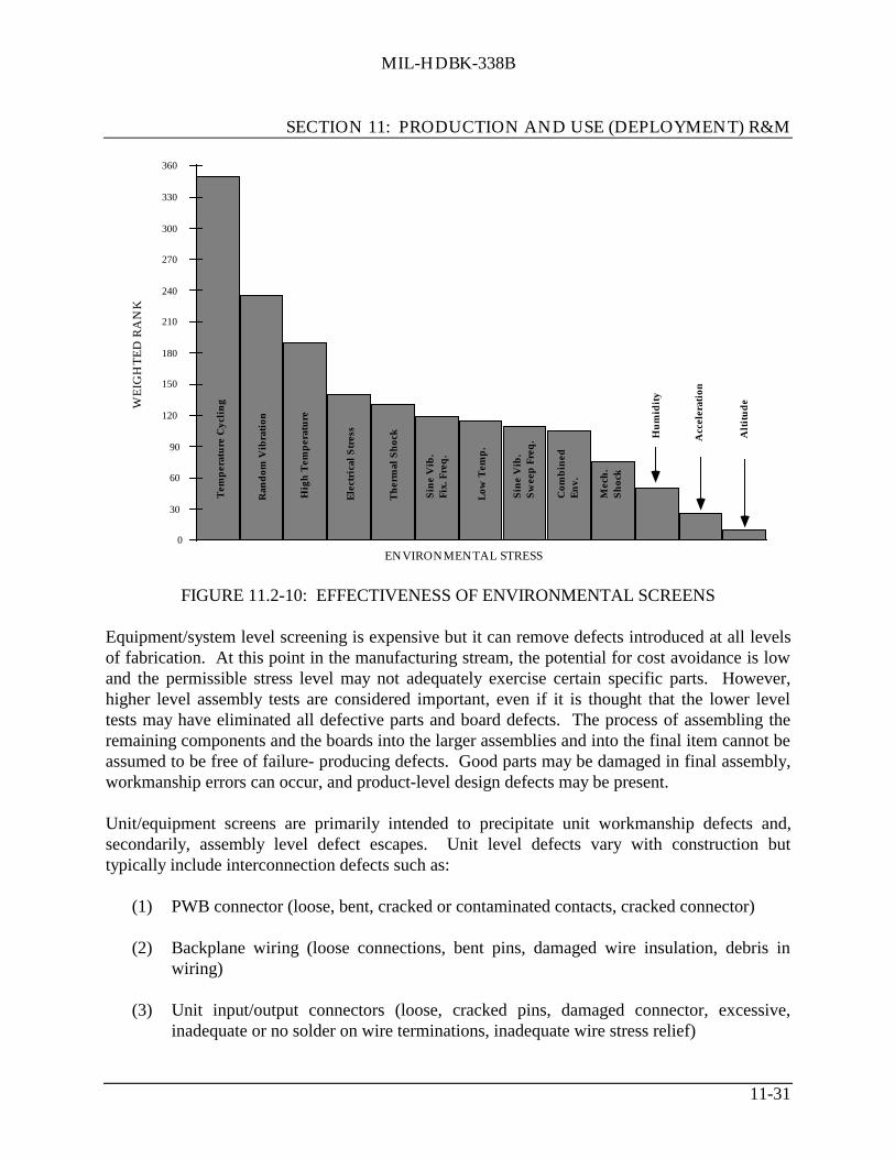
MIL-HDBK-338B


11-31

0

30

60

90

120

150

180

210

240

270

300

330

360

Ran

dom

Vib

rati

on

Hig

h T

emp

erat

ure

Ele

ctri

cal S

tres

s

Th

erm

al S

hoc

k

Sin

e V

ib.

Fix.

Fre

q.

Low

Tem

p.

Sin

e V

ib.

Sw

eep

Fre

q.

Com

bin

ed

En

v.

Mec

h.

Sh

ock

Hu

mid

ity

Acc

eler

atio

n

Alt

itu

de

ENVIRONMENTAL STRESS

WE

IGH

TE

D R

AN

K

Tem

per

atu

re C

ycli

ng

FIGURE 11.2-10: EFFECTIVENESS OF ENVIRONMENTAL SCREENS

Equipment/system level screening is expensive but it can remove defects introduced at all levelsof fabrication. At this point in the manufacturing stream, the potential for cost avoidance is lowand the permissible stress level may not adequately exercise certain specific parts. However,higher level assembly tests are considered important, even if it is thought that the lower leveltests may have eliminated all defective parts and board defects. The process of assembling theremaining components and the boards into the larger assemblies and into the final item cannot beassumed to be free of failure- producing defects. Good parts may be damaged in final assembly,workmanship errors can occur, and product-level design defects may be present.

Unit/equipment screens are primarily intended to precipitate unit workmanship defects and,secondarily, assembly level defect escapes. Unit level defects vary with construction buttypically include interconnection defects such as:

(1) PWB connector (loose, bent, cracked or contaminated contacts, cracked connector)

(2) Backplane wiring (loose connections, bent pins, damaged wire insulation, debris inwiring)

(3) Unit input/output connectors (loose, cracked pins, damaged connector, excessive,inadequate or no solder on wire terminations, inadequate wire stress relief)

MIL-HDBK-338B


11-32

(4) Intra-unit cabling (improperly assembled coax connectors, damaged insulation)

Units may also contain wired assemblies integral to the unit and not previously screened, such asPower Control and BIT Panels, and purchased assemblies, such as modular power supplies.

11.2.3.3 Screen Test Planning and Effectiveness

An effective reliability screening program requires careful planning that starts during earlydevelopment. Tradeoff studies are performed and a complete test specification is prepared andpossibly verified for its effectiveness on prototype hardware.

A key step in specifying an effective screening program is the identification of the kinds offailure modes that can occur and the assembly level at which they may be induced. Theappropriate screens are those which are most effective in accelerating the identified modes,whether they are intrinsic to the part or induced by the manufacturing process.

Due to the varied nature of military electronics equipments and their associated design,development and production program elements, it is difficult to “standardize” on a particularscreening approach. A tailoring of the screening process to the unique elements of a givenprogram is, therefore, required.

Screens should be selected based upon estimates of cost and effectiveness, early developmentprogram data, equipment design, manufacturing, material and process variables, which at leastnarrow consideration to the most cost effective choices. The screening process then should becontinuously monitored and the results analyzed so that changes in the process can be made asrequired to optimize the cost effectiveness of the screening program.

11.2.3.3.1 Environmental Stress Screening per MIL-HDBK-344

MIL-HDBK-344 is organized according to the general sequence of events for planning,monitoring and controlling a screening program. Five detailed procedures are used to assist theuser in accomplishing ESS planning and evaluation activities. The detailed procedures arebriefly described as follows:

Procedure A - Optimizing Screen Selection and Placement

This procedure is used to plan an ESS program such that the required field reliability is attainedat an optimum combined user-producer cost. Procedures B and C are subsequently used todesign the ESS program, and Procedure D is then used to validate the original estimates of defectdensity and screening strength and to redefine the ESS program as necessary.

Five detailed procedures are contained within Procedure A. Procedure A1 creates the basic ESSmodel for a particular program and determines the incoming defect density, allowable outgoing



MIL-HDBK-338B


11-33

defect density based on a reliability requirement, and factory ESS constraints. Procedure A2optimizes the combined user/producer cost of achieving the specified reliability using the resultsof Procedure A3. Procedure A3 calculates the cost of the ESS program. Procedure A4 is used asa precautionary measure to ensure that the ESS is not too stressful and does not consume toomuch of the useful (fatigue) life. Procedure A5 is then used to refine the program, as designedusing procedures A1 through A4, by determining actual values for incomming defects (DIN),screening strength (SS), detection efficiency (DE), and stress adjustment factor (SAF) fromfactory and field data analyzed using Procedure D.

Procedure B - Estimating Defect Density

This procedure is used to estimate the number of defects resident in the system prior to beginningESS. In this procedure the number of defects is defined relative to a baseline stress level.Appropriate factors are then applied to determine the number of defects for different stress levelsof vibration, temperature and temperature transition rates that occur in the factory and the field.It is important to address these stress adjustment factors when planning an ESS program sincethey affect the economic optimization.

The procedure steps are: 1) estimate defects for each assembly and the total system at baselinestress, 2) proportion the defects into random vibration (RV) and temperature cycling (TC)sensitive populations, and 3) apply stress adjustment factors to determine the defects underdifferent factory stress levels. Two procedures are contained within Procedure B. Procedure B1determines the number of latent defects resident in the equipment at the baseline stress.Procedure B2 determines the stress adjustment factor relating defects at factory (baseline stress)levels to defects at the field application stress levels.

Procedure C - Estimating Screening Strength (SS)

This procedure is used to estimate the number of flaws precipitated and detected (removed) byESS. Screening strength is characterized by a precipitation term and a detection term anddetermines the fraction of existing flaws that are removed by ESS. Precipitation is defined as theconversion of a flaw with some residual strength into a flaw with no strength. The application ofstress precipitates a certain fraction of the existing flaws. This fraction is assumed to be constantfor a specific stress level and duration. The removal of a potential defect or flaw requires theflaw to be precipitated and subsequently detected and removed. Detection efficiency is definedas the capability of detecting, isolating and removing the defect once it has precipitated.Precipitation and detection terms are estimated separately and their product determines thescreening strength.

MIL-HDBK-338B


11-34

Procedure D - Refining Estimates of Defect Density and Screening Strength

This procedure is used to provide revised estimates of the ESS modeling parameters (DIN,precipitation efficiency (PE) and SS, DREMAINING, etc.) using actual factory and field data. Themost important parameter for ESS is the defects remaining at the time of shipment since thisdetermines the field reliability. Other significant parameters are the initial defect density, and thescreening strength of the various screens. The difficulty, however, is that none of theseparameters are directly observable by the producer. Only the defects removed through factoryESS can be measured. This procedure provides the means for determining these other criticalparameters from factory data.

Procedure E - Monitor and Control

This procedure is used to implement a program to monitor and control the ESS program(consistent with TQM philosophy) thereby ensuring that the program remains cost effectiveunder the evolving conditions. It provides a quantitative assessment of whether reliabilityrequirements are being attained and to what extent continuous improvement is being realized.The parameters of interest for monitor and control are those determined in Procedure D.Modified SPC and Pareto charts are prepared to monitor these parameters against therequirements which were established in Procedure A.

Procedure F - Product Reliability Verification Test (PRVT)

This procedure is used in conjunction with Procedure E for monitor and control purposes toprovide confidence that field reliability will be achieved. The objective is to retain a minimumESS program so that field reliability can be projected and out-of-control conditions identified.PRVT is defined as that portion of a minimal ESS retained for the purpose of providing amechanism to indicate when the process is not in control and is an inherent part of the ESSprogram.

The product development phase is used to experiment with stress screens, and to then define andplan a cost effective screening program for production. After the screening program isimplemented during production, stress screening results are used to evaluate the screeningprocess to establish whether program objectives are being achieved.

Quantitative objectives for the screening program must be established early. Appendix A of MIL-HDBK-344 contains the mathematical relations and model descriptions used in the Handbook. Areview of Appendix A will help in gaining a quick understanding of the rationale andmethodology of the Handbook. A typical task sequence in Planning, Monitoring and Controllingan ESS Program in accordance with MIL-HDBK-344 is shown in Figure 11.2-11.



MIL-HDBK-338B


11-35

Collect FieldFailure Data

and PostScreening Test

Data

Establish ESS Planand Procedure

Implement ScreenSelection & Placement

Collect Fallout FailureData and PerformFailure Analysis

Modify Screen Selectionand Placement

Does ScreeningFallout CompareFavorably withPlanned Fallout

Is Field LatentDefect Quality

Unacceptably High

Continue to UsePresent ScreeningPlan and Monitor

No

Yes

Obtain Estimateof Latent Defect Quantity

No

Yes

FIGURE 11.2-11: MIL-HDBK-344 ESS PROCESS

MIL-HDBK-338B


11-36

11.2.3.3.2 Tri-Service ESS Guidelines

A Tri-Service Technical Brief 002-93-08, Environmental Stress Screening Guidelines, wasissued in July 1993. The following excerpts from this document provide examples of itstechnical guidance and flexibility.

A viable ESS program must be actively managed, and tailored to the particular characteristics ofthe equipment being screened. A survey should be conducted to determine the mechanical andthermal characteristics of the equipment and refining the screening profiles as more informationbecomes available and/as designs, processes, and circumstances evolve.

Initially, ESS should be applied to all the units manufactured, including repaired units. By usinga closed loop feedback system, information can be collected to eventually determine if thescreening program should be modified.

The following summarizes the ESS guidance:• Define contractual requirements• Identify a general approach• Identify the nature of anticipated defects for unit design and manufacturing processes• Exercise a cost model considering:

- Assembly level at which to apply ESS- Level of automation versus manual labor- Specific rates of thermal change versus capital investment to achieve it

- Adequacy of available in-house random vibration equipment versus cost of off-site screening or the purchase of new equipment

- Cost considerations of active versus passive screening• Review available government and industry data relative to the design of screening

profiles for comparable equipment• Review product design information to identify any thermal characteristics or

mechanical resonances/weakness which could affect screening profiles• Tailor and finalize the temperature cycling screen, at each level of assembly selected,

for temperature limits, rate of temperature change, number of temperature cycles, andwhether monitored during screen

• Tailor and finalize the random vibration screen, at each level of assembly selected, forspectrum, grms level, number of axes, true random or quasi-random, and whethermonitored during screen

• Optimize or modify the ESS profiles based on data from the screens or from operationaluse

• Consider sampling for the ESS screen based on screening data collected, but only withcustomer concurrence.



MIL-HDBK-338B


11-37

11.2.3.3.2.1 Types of Flaws to be Precipitated

Based on the types of failures expected in the equipment, Table 11.2-4 provides information thatcan be used to help establish the unique equipment profile. Care must be taken that in tailoringthe screening environment to one type of failure, other types of failures do not go undetected.

TABLE 11.2-4: SCREENING ENVIRONMENTS VERSUS TYPICALFAILURE MECHANICS

SCREENING ENVIRONMENT - TYPE OF FAILURE

THERMAL CYCLING VIBRATIONTHERMAL ORVIBRATION

• Componentparameter drift

• Particle contamination • Defective solderjoints

• PCB opens/shorts • Chaffed, pinched wires • Loose hardware• Component

incorrectlyinstalled

• Defective crystals • Defectivecomponents

• Wrongcomponent

• Mixed assemblies • Fasteners

• Hermetic sealfailure

• Adjacent boards rubbing • Broken component

• Chemicalcontamination

• Two componentsshorting

• Improperly etchedPCBs

• Defective harnesstermination

• Improperly seatedconnectors

• Surface mounttechnology flaws

• Improper crimp • Poorly bondedcomponent

• Poor bonding • Inadequately securedparts

• Hairline cracks inparts

• Mechanical flaws

• Out-of-toleranceparts

• Loose wire

11.2.3.3.2.2 Levels of Assembly at which ESS may be Performed

The term piece part, as used here, is defined as a monolithic integrated circuit, resistor, switch,etc., that is the lowest level of assembly. The next level of assembly is a multi-part assembly thathas a defined identity e.g., one that is given a drawing number and, usually, a name. A typicalitem at this level is a printed wiring assembly (PWA), shop replaceable assembly (SRA), or shopreplaceable unit (SRU). The top level is a system. In reality, there is always some aggregate

MIL-HDBK-338B


11-38

that is the largest entity reasonably possible to subject to ESS, and there usually are several levelsof assembly at which ESS can be considered.

It is more cost effective to do ESS at the lowest level possible and at more than one level. Thechoices of how many levels and which levels are made on the basis of an engineering evaluation.

The costs associated with a failure usually appear in connection with a single part orinterconnection and will increase dramatically with the level of assembly. Consider that:

• At higher levels- More assembly work has to be undone and redone when failures occur- More material may need to be scrapped- More impact on production flow and schedule usually occurs

• At lower levels- Corrective action is quicker

In view of the preceding, it is understandable that the tendency is to perform ESS at lower levelsof assembly. However, each step in assembly and integration provides additional opportunitiesfor the introduction of flaws. Obviously, ESS at a particular level cannot uncover flaws that arenot introduced until the next level. Generally, this dilemma is usually controlled by performingESS at each major functioning level in the manufacturing process consistent with an assessmentof the defect population at each level of assembly.

To resolve these conflicting considerations, screening is usually done at multiple (usually 2 or 3)levels of assembly. ESS at lower levels should focus on precipitating and correcting flaws inpiece parts and PWA processing. Most ESS failures at higher levels will reflect flaws introducedlater in the manufacturing sequence that are usually correctable without tear-down to a lowerlevel. Table 11.2-5 provides a summary of the risks and results of doing ESS at various levels.



MIL

-HD

BK

-338

B

SEC

TIO

N 1

1: P

RO

DU

CT

ION

AN

D U

SE (D

EPL

OY

ME

NT

) R&

M

11-3

9

TA

BL

E 1

1.2-

5: R

ISK

S A

ND

RE

SUL

TS

OF

ESS

AT

VA

RIO

US

LE

VE

LS

ESS

CO

ND

ITIO

NS

/ TR

AD

EO

FFS

RIS

KS

/ EFF

EC

TS

Lev

el o

fA

ssem

bly

Pow

erA

pplie

d 1

I/O

2M

onito

red3

ESS

Cos

tT

echn

ical

Com

men

tsY

esN

oY

esN

oY

esN

oR

isk

Res

ults

TE

MP

ER

AT

UR

E C

YC

LIN

GX

XX

Low

Low

Poo

rC

ondu

ct P

re &

Pos

t ESS

fun

ctio

nal t

est

PW

AX

XX

Hig

hL

ower

Bet

ter

scre

en p

rior

to c

onfo

rmal

coa

ting

XX

XH

ighe

stL

owes

tB

est

XX

XH

ighe

stL

owes

tB

est

If c

ircu

mst

ance

s pe

rmit

ESS

at o

nly

one

Uni

t/Box

XX

XL

ower

Hig

her

Goo

dle

vel o

f as

sem

bly

impl

emen

t at u

nit l

evel

XX

XL

owes

tH

ighe

stP

oor

Syst

emX

XX

Hig

hest

See

Com

men

tM

ost

effe

ctiv

e E

SS

at

syst

em

leve

l is

sh

ort

dura

tion

rand

om v

ibra

tion

to l

ocat

e in

ter-

conn

ect

defe

cts

resu

lting

from

sys

tem

inte

grat

ion.

RA

ND

OM

VIB

RA

TIO

NX

XX

Hig

hest

Low

Goo

dR

ando

m v

ibra

tion

can

be e

ffec

tive

at P

CB

leve

l if:

1. S

urfa

ce M

ount

Tec

hnol

ogy

is U

tili

zed

PW

AX

XX

Hig

hH

igh

Fair

2. P

WA

has

larg

e co

mpo

nent

sX

XX

Low

Hig

hest

Poo

r3.

PW

A is

mul

tilay

er4.

PW

A c

anno

t be

effe

ctiv

ely

scre

ened

at

high

eras

sem

blie

sX

XX

Hig

hest

Low

Bes

tR

ando

m v

ibra

tion

mos

t ef

fect

ive

at t

his

leve

l of

ass

embl

y.In

term

itten

t fla

ws

mos

t sus

cept

ible

Uni

t/Box

XX

XL

owH

ighe

rG

ood

to p

ower

-on

with

I/O

ESS

. Pow

er-o

nX

XX

Low

est

Hig

hest

Poo

rw

ithou

t I/

O r

easo

nabl

y ef

fect

ive.

Dec

isio

n re

quir

es c

ost

bene

fit t

rade

off.

Sys

tem

XX

XL

owL

owG

ood

Cos

t is

rel

ativ

ely

low

bec

ause

pow

er a

nd I

/O n

orm

ally

pres

ent d

ue to

nee

d fo

r ac

cept

ance

test

ing.

NO

TE

S to

Tab

le 1

1.2-

5:1.

Pow

er a

pplie

d -

At P

WA

leve

l of

asse

mbl

y, p

ower

on

duri

ng E

SS is

not

alw

ays

cost

eff

ectiv

e.2.

I/O

- E

quip

men

t ful

ly f

unct

iona

l with

nor

mal

inpu

ts a

nd o

utpu

ts3.

Mon

itore

d -

Mon

itori

ng k

ey p

oint

s du

ring

scr

een

to a

ssur

e pr

oper

equ

ipm

ent o

pera

tion

MIL-HDKB-338B


11-40

11.2.3.3.2.3 Types and Severities of Stresses

A variety of environmental stresses have been considered for use in ESS over the years. Ofthese, random vibration and thermal cycling currently are considered to be the most costeffective. Table 11.2-4 identifies some common types of failures and reflects whether randomvibration or thermal cycling is the more likely stress to precipitate that particular failure. Afailure may be precipitated by one stress, but detected under another.

Traditional ESS, consisting of temperature cycling and random vibration, may not be the mosteffective. For example, power cycling is effective in precipitating certain types of latent defects;pressure cycling may be desirable for sealed equipment; and acoustic noise may excitemicroelectronics structures better than structure-borne vibration. Ultimately, ESS environmentsmust be chosen based on the types of flaws that are known or expected to exist.

In the past, fixed-frequency or swept-sine vibration testing was sometimes used. These practiceswere attributable in part to costs and physical limitations of available test equipment at the time.The shortfalls of fixed frequency and swept-sine vibration in comparison with broadband randomvibration were not known at the time. Today, random and quasi-random vibration are usedalmost exclusively for ESS. It is not difficult to visualize that the complex interactions possibleunder random vibration can induce a wider variety of relative motions in an assembly.

Burn-in has been defined many ways by different agencies and companies; however, it is mostfrequently defined as the exposure of powered equipment to either ambient or elevatedtemperature. Burn-in is not adequate for detecting flaws.

Effective screening requires large, rapid temperature changes and broadband random vibration.Such thermal cycling is used for the detection of assembly flaws that involve installation errorsor inadequate chemical or mechanical isolation or bonding. Under rapid thermal cycling,differential thermal expansion takes place without sufficient time for stress relief, and is a majormechanism for precipitating latent defects.

It is important to note that thermal cycling and random vibration are synergistic. For example,thermal cycling following random vibration sometimes leads to detection of vibration-inducedfailures that were not immediately apparent. In reported cases, vibration stressing had caused aflawed conductor to break, but the loss of continuity only became evident with temperaturechange. In other cases, a very small flaw may not propagate to the point of detectability duringrandom vibration but may advance to the point of detectability during subsequent thermalcycling.



MIL-HDBK-338B


11-41

The concurrent application of the vibration and thermal cycling may be desirable, but is oftenavoided because it requires more elaborate facilities and makes it more difficult to provide thedesired capabilities for functional checking during ESS. Also, concurrent application of randomvibration and thermal cycling can make it difficult to determine what caused a defect so thatcorrective action can be taken. If random vibration and thermal cycling are conductedsequentially, random vibration should be done first.

11.2.3.3.2.4 Failure Detection Measurements During Thermal Cycling and RandomVibration

Two approaches are used to monitor equipment during thermal cycling. In the first approach,limited performance measurements are made prior to and at the end of ESS. These performancemeasurements may be made on the first and last cycle. Additional measurements may be taken atother cycles, if desired. Each measurement should be made at the hot and cold operatingextremes.

In the second approach, equipment operation is continuously monitored during the cold-to-hottransition and during the hot dwell portion of each cycle.

The argument for monitoring equipment during vibration screens is that the resulting movementof a marginal component may show up as an equipment failure only during the stress application.Otherwise, the incipient failure will escape detection, only to show up in an operationalenvironment. Some of the initial work in random vibration screening indicated a 2:1 differencein the efficiency of the screen if the equipment were powered and monitored versus not powered.The technical risks and costs are summarized in Table 11.2-5 at each level of assembly forrandom vibration screening.

11.2.3.3.2.5 Baseline ESS Profiles

The baseline profiles (Tables 11.2-6 and 11.2-7) represent the combined agreement of the threemilitary services on minimum levels to ensure effectiveness. The profiles are based onexperimental and analytical stress screening studies and surveys of screens used in industry. Therandom vibration baseline profile given in Table 11.2-6 shows a range of recommendedminimum acceptable values for input levels, frequencies, axes, duration and monitoring. Thethermal cycling baseline profile given in Table 11.2-7 shows a range of recommended values forthe temperature extremes, the temperature rate of change and the number of cycles.

MIL-HDKB-338B


11-42

TABLE 11.2-6: BASELINE VIBRATION PROFILE

LEVEL OF ASSEMBLYCHARACTERISTIC PWA 1 UNIT SYSTEM

Overall Response Level 2 6g RMS 6g RMS 6g RMS

Frequency 3 20 - 2000 Hz 20 - 2000 Hz 20 - 2000 HzAxes 4

(Sequentially or Simultaneous)3 3 3

Duration- Axes Sequentially 10 minutes/axis 10 minutes/axis 10 minutes/axis- Axes Simultaneously 10 minutes 10 minutes 10 minutesProduct Condition Unpowered

(Powered if purchased asan end item deliverable oras a spare)

Powered,Monitored

Powered,Monitored

NOTES: Pure random vibration or Quasi-random vibration are considered acceptable forms of vibration for thepurpose of stress screening. The objective is to achieve a broad-band excitation.

1. When random vibration is applied at the unit level, it may not be cost effective at thePWA level. However, PWAs manufactured as end item deliverables or spares mayrequire screening using random vibration as a stimulus. However, at the system level,when a response survey indicates that the most sensitive PWA is driving the profile ina manner that causes some PWAs to experience a relatively benign screen, that PWAshould be screened individually. Each PWA screened separately should have its ownprofile determined from a vibration response survey.

2. The preferred power spectral density for 6g rms consists of 0.04g2/Hz from 80 to 350Hz with a 3 dB/octave rolloff from 80 to 20 Hz and a 3 dB/octave rolloff from 350 to2000 Hz.

3. Vibration input profile for each specific application should be determined by vibrationresponse surveys which identify the correlation between input and structural responses.Higher frequencies are usually significantly attenuated at higher levels of assembly.

4. Single axis or two axis vibration may be acceptable if data shows minimal flawdetection in the other axes.



MIL-HDBK-338B


11-43

TABLE 11.2-7: BASELINE THERMAL CYCLE PROFILE

LEVEL OF ASSEMBLYCHARACTERISTIC1 PWA 2 UNIT 3 SYSTEM

Temperature Range ofHardware

-50°C to +75°C -40°C to +70°C -40°C to +60°C

Temperature Rate of Changeof Product 4

15°C/minuteto 20°C/minute



Stabilization Criterion Stabilization has occurred when the temperature of theslowest-responding element in the product being screened iswithin ±15% of the specified high and low temperatureextremes. Large magnetic parts should be avoided whendetermining that stabilization has occurred. 5

Soak Time of Hardware at Temperature Extremes after Stabilization- If Unmonitored 5 minutes 5 minutes 5 minutes- If Monitored Long enough to perform functional testing

Number of cycles 20 to 40 12 to 20 12 to 20Product Condition 6 Unpowered Powered,

MonitoredPowered,Monitored

NOTES:1. All temperature parameters pertain to the temperature of the unit being screened and

not the chamber air temperature. The temperature parameters of the unit beingscreened are usually determined by thermocouples placed at various points on the unitbeing screened.

2. PWA guidelines apply to individual PWAs and to modules, such as flow-throughelectronic modules consisting of one or two PWAs bonded to heat exchanger.

3. Unit guidelines apply to electronic boxes and to complex modules consisting of morethan one smaller electronic module.

4. Hardware temperature rate of change is limited to capabilities of ESS chambers. Thechamber temperature rate of change is optimized to approach the hardwaretemperature rate of change. This is best accomplished through a series of thermalsurveys.

5. It is up to the designer of the screening profile to decide which elements of thehardware (parts, solder joints, PWAs, connectors, etc.) must be subjected to theextreme temperatures in the thermal cycle. The temperature histories of the variouselements in the hardware being screened are determined by means of a thermalsurvey.

6. Power is applied during the low to high temperature excursion and remains on untilthe temperature has stabilized at the high temperature. Power is turned off on thehigh to low temperature excursion until stabilization at the low temperature. Power isalso turned on and off a minimum of three times at temperature extremes on eachcycle.

MIL-HDKB-338B


11-44

These minimum acceptable baseline profiles for random vibration and temperature cycling arenot recommended stress levels, but are starting points for developing unique optimum profilesfor a particular configuration.

The most significant conclusion from ten years of random vibration screening is that theexcitation must be tailored to the response experienced by the components of the unit under test.The selection of stress levels must be based on available data and structural design. To avoidpotential fatigue or peak level damage due to resonances, some level reduction of the inputspectrum may be done at points of severe resonant frequencies (i.e., those which result inamplification of the applied stress level by a factor of 3 dB or more.). These resonances wouldbe obtained from data accumulated during development tests, or by conducting a low-level sinesweep. Where warranted, temporary stiffening of the unit should also be considered to preventoverstressing during the stress screen. The stiffening should be done in a manner which achievesthe desired flat response throughout the unit being screened.

The temperature cycling screens also have to be tailored to each specific equipment and areequipment unique. Differences in components, materials and heat dissipation lead to variationsin the thermal stresses throughout the item.

11.2.3.3.2.6 Optimizing/Tailoring of ESS

For any given part or production process, there exists a level of ESS stress that is optimal, i.e.,maximizes the likelihood of flaw detection without significant degradation of the unit undergoingESS. ESS tailoring (modification of ESS parameters to fit specific hardware), if not planned anddone properly, could be a major expense. Experience with similar hardware can be helpful insetting initial tailoring levels leading to a rough approximation of optimal parameters. However,a true optimization is likely to require an extensive, carefully planned effort.

Recommended tailoring techniques are given in Sections 4 and 5 of the tri-service ESSguidelines for vibration screens and thermal cycling screens, respectively. These are not the onlytechniques available but are recognized throughout the industry as starting points for anacceptable profile. The selection and use of one or more of these techniques is usually predicatedon such things as availability of screening equipment or cost of procurement, architecture ofequipment to be tested, type of manufacturing defects expected, and maturity of design andmanufacturing processes. Trade-offs are needed because the payoff between reasonably goodand optimal ESS parameters may not be commensurate with the costs of finding the optimalprofile.

Some specific engineering considerations in determining optimal ESS stress levels and making asound engineering decision that tends to be on the conservative side (i.e., no overstressing) are asfollows:

• Differences in physical characteristics such as thermal inertia, thermal conductivity,



MIL-HDBK-338B


11-45

mechanical coupling, and mechanical resonant frequencies assure that differentlyconfigured assemblies will respond differently to identical thermal and vibrationalinputs.

• Stress profiles should be defined in terms of responses rather than input, especially forvibration. A uniform level of stress may not be achieved throughout the unit, becauseunits are not generally internally homogeneous. The response can be specified andmeasured at only a few points, so it will still differ locally within differently configuredassemblies.

There are various approaches associated with the application of stress screens. Regardless of theapproach used, the fundamental objective of ESS remains the same, i.e., to remove latent defectsfrom the product prior to field delivery. The quantitative methods contained in MIL-HDBK-344and the tri-service ESS guidelines extend this objective by focusing on the defects which remainin the product at delivery and their impact on field reliability.

11.2.4 Production Reliability Acceptance Testing (MIL-HDBK-781)

Reliability acceptance testing is performed on production hardware to determine compliance tospecified reliability requirements. MIL-HDBK-781, “Production Reliability Acceptance Testing”contains all the essential procedures and requirements for designing an acceptance test plan forequipment that experiences a distribution of times-to-failure that is exponential. It defines testconditions, procedures and various test plans, and respective accept/reject criteria.

MIL-HDBK-781 has recently been completely revised to include detailed information for testplanning and evaluation of data. The latest revision has been restructured to make extensive useof appendices to expand and clarify the various sections of the handbook. It clarifies thedefinition of mean-time-between-failures (MTBF) and the use of θ0 (upper test MTBF) and

θ1 (lower test MTBF) , which are test planning parameters, and specifies the use of combined

environmental test conditions (temperature, vibration and moisture)* based on the actual missionprofile environments encountered during the equipment's useful life.

MIL-HDBK-781 is not intended to be used on a blanket basis, but each requirement should beassessed in terms of the need and mission profile. Appendices are designed so that the procuringactivity may reference them along with specific parts of the handbook.

MIL-HDBK-781 covers requirements for preproduction qualification tests as well as productionacceptance tests. Qualification tests are normally conducted after growth tests in the developmentcycle, using initial production hardware to make a production release decision. It should be

* Altitude may be included if the procuring activity determines that it is cost effective, but the cost of

test facilities for combining altitude with the other environments would probably be prohibitive.

MIL-HDKB-338B


11-46

emphasized that qualification testing, conducted per MIL-HDBK-781, is to demonstratereliability with statistical confidence, whereas reliability growth testing is performed to improvereliability. Depending on program requirements, funding, and other constraints, preproductiontesting may maximize growth testing and minimize statistical testing (resulting in a high MTBFat a low confidence) or may minimize growth and maximize demonstration (resulting in a lowerMTBF at a high confidence). Preproduction testing, including both reliability growth andqualification, was discussed in detail in Section 8.

Production reliability acceptance tests per MIL-HDBK-781 are described as “a periodic series oftests to indicate continuing production of acceptable equipment” and are used to indicateindividual item compliance to reliability criteria. The tests are intended to simulate in-serviceevaluation of the delivered item or production lot and to provide verification of the inherentreliability parameters as demonstrated by the preproduction qualification tests. Therefore, anequipment would undergo qualification testing on preproduction hardware.

Once the specified reliability has been demonstrated, and after production begins, the lotsproduced would undergo reliability acceptance testing, usually at a stress less stringent than thedemonstration test level, to indicate continuing fulfillment of reliability requirements.

Production Reliability Acceptance Testing per MIL-HDBK- 781 can be performed based onsampling an equipment from each lot produced as well as on all equipment produced. The testconditions, or stress profile, applied during the test should be measured (preferred) or estimatedby the procuring activity and incorporated into the equipment specification. However, when thestress types and levels are not specified by the procuring activity and when measuredenvironmental stresses for the proposed application or a similar application are not available forestimating, then the stress types and levels given in Table 11.2-8, taken from MIL-HDBK-781,should be applied. Table 11.2-8 provides a summary of combined environmental test conditionrequirements applicable to the following categories of equipment classification:

Category 1: Fixed ground equipment

Category 2: Mobile ground vehicle equipment

Category 3: Shipboard equipment- sheltered- unsheltered

Category 4: Equipment for jet aircraft

Category 5: Turbo-prop aircraft and helicopter equipment

Category 6: Air-launched weapons and assembled external stores



MIL-HDBK-338B


11-47

Figure 11.2-12, also taken from MIL-HDBK-781, illustrates a typical test cycle that shows thetiming of the various conditions. MIL-HDBK-781 describes standard statistical test planscovering:

(1) Fixed length test plans (Test Plans IXC through XVIIC and XIXC through XXIC)

(2) Probability ratio sequential tests (PRST) (Test Plans IC through VIC)

(3) Short run high risk PRST plans (Test Plan VIIC and VIIIC)

(4) All equipment reliability test (Test Plan XVIIIC)

Accept/reject criteria are established on θ1 and θ0 , where θ1 , the lower test MTBF, is an

unacceptable MTBF based on minimum requirements. θ0 is the upper test MTBF, or the

acceptable MTBF. The ratio θ0 /θ1 is defined as the discrimination ratio. Specifying any two of

these three parameters, given the desired producer and consumer decision risks, determines thetest plan to be utilized.

Test Plan XVIIIC, shown in Figure 11.2-13, can be used for 100% production reliabilityacceptance testing. This test plan is to be used when each unit of production (or preproductionequipment if approved by the procuring activity) equipment is to be given a reliability acceptancetest. The plan consists of a reject line and a boundary line. The reject and boundary lines areextended as far as necessary to cover the total test time required for a production run. Theequation of the reject line is fR = 0.72T + 2.50 where T is cumulative test time in multiples of

θ1 and f is cumulative number of failures. The plotting ordinate is failures and the abscissa is in

multiples of θ1 , the lower test MTBF. The boundary line is 5.67 failures below and parallel to

the rejection line. Its equation is fB = 0.72T - 3.17.

The test duration for each equipment shall be specified in the test procedure as approved by theprocuring activity. The maximum duration may be 50 hours and the minimum 20 hours to thenext higher integral number of complete test cycles. If a failure occurs in the last test cycle, theunit shall be repaired and another complete test cycle run to verify repair.

An optional nonstatistical plan can also be used for production reliability acceptance testing. Itspurpose is to verify that production workmanship, manufacturing processes, quality controlprocedures, and the assimilation of production engineering changes do not degrade the reliability,which was found to be acceptable by the reliability qualification test. The test is to be applied toall production items with the item operating (power applied). The required test duration andnumber of consecutive, failure free, thermal test cycles (minimum of two) which each deliverable

MIL-HDKB-338B


11-48

item must exhibit is specified by the procuring activity. The vibration, temperature cycling, andmoisture environments together with any others which are deemed necessary may be appliedsequentially. The equipment duty cycle and the sequence, duration, levels of the environments,and the vibration option to be used in this test require approval of the procuring activity and aresubmitted in accordance with the test program requirements.

TABLE 11.2-8: TEST CONDITIONS MATRIX (TAKEN FROM MIL-HDBK-781)

Summary of Combined Environmental Test Condition RequirementsFIXED GROUND SHIPBOARD

GROUND VEHICLE SHELTERED UNSHELTEREDELECTRICAL STRESS

Input voltageVoltage cycle

Nominal +5%-2%high, nominal and →low

Nominal ± 10%one per test cycle

Nominal ±7%*

Nominal ± 7%*→

VIBRATION STRESSType vibration

AmplitudeFrequency range***Application

sinewavesingle frequency(See APPENDIX B for20 to 60 Hz20 minimum per equipment

swept-sinelog sweepstress levels)5 to 500 Hzsweep rate15 minimum once/hr.

swept-sine **continuous

(See APPENDIX B

swept-sine**continuous

→)

THERMAL STRESS (°C)Storage temperatureOperating temperatureRate off changeMaximum rate of change

A B C ****- - -20 40 60- - -- - -

LOW HIGH-54 85-40 TO555°/min.10°/min.

LOW HIGH-62 710 TO 50 (CONTROLLED)5°/min.10°/min.

LOW HIGH-62 71-28 655°/min.10°/min.

MOISTURE STRESSCondensationFrost/freeze

none 1/test cycle1/test cycle

See APPENDIX B 1/test cycle1/test cycle

AIRCRAFT AIR-LAUNCHED

FIGHTERTRANSPORT,

BOMBER HELICOPTER TURBO-PROP

WEAPONS ANDASSEMBLED

EXTERNAL STORESELECTRICAL STRESS

Input voltage rangeVoltage cycle

nominal ± 10%(nominal, high and

± 10%low voltage, one cycle

± 10%/thermal cycle or per

± 10%APPENDIX B)

± 10%

VIBRATION STRESSType vibrationAmplitudeFrequency rangeApplication

random(200 - 2000 Hzcontinuous

random SEE20 - 2000 Hzcontinuous

swept-sine log-sweepAPPENDIX B 5 - 2000 Hz****sweep rate15 min. one/hr

swept-sine10 - 2000 Hzcontinuous(See APPENDIX B)

swept-sine***→ )20 - 2000 Hzcontinuous(See MIL-STD-1670)

THERMAL STRESS (°C)Storage temperature (non-oper.)Operating temperature rangeRate of change (min.)Duration (nominal)

LOW HIGH-54 +71(←5°/min.3 1/2 hours

LOW HIGH-54 +71 SEE APPENDIX5°/min.3 1/2 hours

LOW HIGH-54 +71B 5°/min.3 1/2 hours

LOW HIGH-54 +715°/min.3 1/2 hours

LOW HIGH-65 +71→)

MOISTURE STRESSCondensationFrost/freeze

(1/test cycle ----------(1/test cycle ----------

--------------------------------------------------

--------------------------------------------------

--------------------------------------------------

---------------------------)---------------------------)

* See MIL-STD-1399** See MIL-STD-167-1*** Frequency tolerance ±2 percent or ±0.5 Hz for frequencies below 25 Hz.**** See 50.1.4 of Appendix B



MIL-HDBK-338B


11-49

DUTY CYCLE

HIGH LOW

ON

OFF

ON

OFF

PRIME VOLTAGE

VIBRATION

EQUIPMENT OPERATION

A B C

Cooling Period

Heating Period Cooling Period

HIGHER TEMPERATURE

TEMPERATURE (°C)

LOWER TEMPERATURE

Time (Hrs.)

Equipment off (can be operated if required) Equipment operated in accordance with duty cycle

Applies to temperature cycle

A. Time for chamber to reach stabilization at higher temperature B. Time of equipment operation at higher temperature C. Optional Hot Soak and hot start-up checkout

FIGURE 11.2-12: SAMPLE ENVIRONMENTAL TEST CYCLE

MIL-HDKB-338B


11-50

5 10 15 20 25

5

10

15

TO

TA

L N

UM

BE

R O

F FA

ILU

RE

S

TEST TIME (IN MULTIPLES OF LOWER TEST TIME, θ )1

REJECT

ACCEPT AND CONTINUE TEST

REJECT LINE

BOUNDARY LINE

f = .72T - 3

.17

B

f= .72T + 2.50

R

Total Test Time*

Number ofFailures

Reject(Equal or less)

BoundaryLine

0 N/A 4.401 N/A 5.792 N/A 7.183 .70 8.564 2.08 9.945 3.48 11.346 4.86 12.727 6.24 14.108 7.63 15.49

Total Test Time*

Number ofFailures

Reject(Equal or less)

BoundaryLine

9 9.02 16.8810 10.40 18.2611 11.79 19.6512 13.18 21.0413 14.56 22.4214 etc. etc.15 . .16 . .. . .

* Total test time is total unit hours of equipment on time and is expressed in multiples of the lower MTBF. Refer to4.5.2.4 for minimum test time per equipment.

FIGURE 11.2-13: REJECT-ACCEPT CRITERIA FOR TEST PLAN XVIIIC



MIL-HDBK-338B


11-51

It must be emphasized that test criteria, including confidence level or decision risk, should becarefully selected and tailored from these documents to avoid driving cost or schedule withoutimproving reliability. Some general guidelines, taken from MIL-HDBK-781 for planning andimplementing production reliability acceptance testing are as follows:

• Production reliability acceptance testing must be operationally realistic, and may berequired to provide estimates of demonstrated reliability.

• The statistical test plan must predefine criteria of compliance ("accept") which limit theprobability that the item tested, and the lot it represents, may have a true reliability lessthan the minimum acceptable reliability. These criteria must be tailored for cost andschedule efficiency.

• Production reliability acceptance testing provide a basis for positive and negativefinancial feedback to the contractor, in lieu of an in-service warranty.

• Production reliability acceptance testing may require expensive test facilities tosimulate the item life profile and operational environment; therefore, all equipmentproduction reliability acceptance testing (100% sampling) is not recommended.

• Because it provides a basis for determining contractual compliance, and applies to theitems actually delivered to operational forces, production reliability acceptance testingmust be independent of the supplier, if at all possible.

• Sampling frequency should be reduced after a production run is well established,however, the protection that it provides for the government (and the motivation itprovides for the contractor's quality control program) argues against complete waiver ofthe production reliability acceptance testing requirement.

Plans for performing production reliability acceptance testing are incorporated into the overallreliability test plan document, and should encompass the following considerations:

(1) Tests to be conducted

(2) Reliability level (i.e., MTBF) to be demonstrated, as well as the associated confidencelevel, and the relationship between demonstrated MTBF, confidence, test time, etc.

(3) Representative mission/environmental profile

(4) The number of units for test, expected test time, calendar time factors, and schedulingof effort

MIL-HDBK-338B


11-52

(5) The kinds of data to be gathered during the test

(6) Definition of failure (relevant, nonrelevant)

(7) Authorized replacement and adjustment actions

(8) Logs/data forms to be maintained that record number of units on test, test timeaccumulated, failures, corrective actions, statistical decision factors, and accept/rejectcriteria

11.2.5 Data Collection and Analysis (During Production)

The production reliability test and control program, once implemented in the factory, shouldcontinually be challenged relative to the effectiveness of the overall program, as well as that ofthe individual tests. Production screening and acceptance testing is a dynamic process whichmust be continually modified in response to experience. Test results and field experience dataare monitored to determine the need to modify individual test criteria and conditions to reducethe sampling frequency of acceptance tests and to identify the possibility of applying earlierscreen tests where the test costs are less and the potential for cost avoidance is higher. It shouldbe emphasized that the production program, as initially planned, represents a baseline forapplying the tests. A production screen test, for example, like any quality inspection, must beadjusted depending on the results of subsequent higher level tests or field performance.However, the extent and nature of any changes should be determined only through careful reviewand analysis of the subsequent failures.

A data system supported by failure analysis and corrective action is established to maintainvisibility over the effectiveness of the production test program as well as all tests includingdevelopment, qualification, and production. The data system is designed to compile test andfailure data and to provide information that would provide a basis to change the test program asnecessary to minimize cost and maximize effectiveness. A failure reporting, analysis andcorrective action system (FRACAS) is an essential element of the production test program aswell as the overall reliability control program. A well designed FRACAS system will provide auniform mechanism for reporting failures, determining causes and remedies, and making thesefindings known to the appropriate engineers and designers to enable them to formulate andimplement corrective action and, specifically, to ascertain whether or not to design andimplement improved inspection, screening and acceptance tests.

Section 8 of the handbook describes failure reporting, analysis, corrective action, and theprovisions necessary to assure that failures are accurately reported, thoroughly analyzed, and thatcorrective actions are taken on a timely basis to reduce or prevent recurrence.

The results of production acceptance test, screening and inspection results, as well as failurereports and analyses from the FRACAS program, are compiled and incorporated into the data



MIL-HDBK-338B


11-53

system. Maintaining accurate and up-to-date records through a formal data recording and analysissystem is particularly essential in tracking and assessing field reliability performance.Comparative evaluation between predicted reliability estimates and actual field reliabilityprovides criteria for improving production acceptance testing (including the screening and burn-in testing procedures) to assure that the most cost effective test program is developed andapplied. This is especially important for new systems where changing performance andreliability characteristics would be expected as a result of design and manufacturingimprovements.

A properly designed and operating data system would provide the following information as itpertains to production testing:

(1) Identification of hardware subjected to production tests

(2) Total cumulative operating time for each hardware item including the last operatingtime interval of failure free operation and acceptance test completion dates

(3) Sampling frequency of reliability acceptance tests

(4) Failure reports of hardware discrepancies including description of failure effects andaccumulated operating hours to time of failure

(5) Failure analysis reports of hardware discrepancies including cause and type of failuremodes

Also, cumulative plots of screening and burn-in failure events versus time can be prepared andmaintained and periodic summary reports submitted to engineering and management activitiesthat provide:

(1) Failure/reject rates by test type and level

(2) Screen test efficiency factors

(3) Responsible failure mechanisms

(4) Recommended or accomplished corrective actions

(5) General product reliability analysis that correlates design predictions with test resultsand field experience of parts, contamination of surfaces or materials, poor soldering ofparts, improper securing of component elements, and bending or deformation ofmaterials

MIL-HDBK-338B


11-54

These defects, as mentioned earlier, whether intrinsic to the parts or introduced during fabricationcan be further isolated into quality and reliability defects. Quality defects are not time dependentand are readily removed by conventional quality control measures (i.e., inspections and tests).The more efficient the inspection and test the more defects that are removed. However, since notest or inspection is perfect, some defects will escape to later manufacturing stages and then mustbe removed at a much higher cost or, more likely, pass through to field use and thus result inlower actual operational reliability with higher maintenance cost.

11.2.6 Monitor/Control of Subcontractors and Suppliers

The monitoring of subcontractors is a critical, but often overlooked function of a successfulreliability program. End product reliability and its life cycle cost can be adversely affected if asub-tier vendor or major subcontractor does not fully comply with the applicable reliabilityprogram requirements.

The requirements for the monitoring of subcontractors and the monitoring of suppliers oftendiffers due to the nature of the product being furnished and may therefore frequently be definedseparately.

11.2.6.1 Major Subcontractor and Manufacturer Monitoring

Development-phase subcontractor monitoring is accomplished by reviewing design data,reliability data, parts selection, non-standard parts requests, failure reports, periodic attendance atdesign reviews and participation in reliability problem resolution. Production-phase monitoringconsists of verifying adherence to the Quality Assurance (QA) standard established between theprime contractor and the subcontractor. It should include the review of process control,production control, personnel qualifications, workmanship and participation in the FRACAS (seesection 8.2).

Normally, except for off-the-shelf procurements, the requirements imposed on the manufacturerof a unit/major assembly is as specified in the prime item/system specification.

Supplier monitoring/control requires detailed inspection of the material being furnished,verification of QA procedures, critique of manufacturing processes, periodic inspection to verifyadherence to the quality standard, identification of problems, incoming inspection, testing andperformance tracking.

Monitoring of Parts Suppliers requires review of vendor performance in addition to the tasksnoted.

11.2.6.2 Establishing Vendor Capability and Program Reviews

The most direct method of determining a vendor capability is to review past performance. If this



MIL-HDBK-338B


11-55

data is not available or is incomplete, a facility survey should be performed.

Program reviews should be conducted on a continuous basis for the life of the contract. It isessential to develop a free exchange of information and data so that the prime contractor hasmaximum program visibility into a vendor’s process methods and performance. These reviewsverify that the manufacturing process is under control, and that: workmanship, personnelcertification training, and testing, as defined in the equipment specification and QA manual, isbeing implemented correctly.

Failure report data from production tests (Burn-in, ESS, PRAT, etc.) received from a vendor oras a result of in-house testing should be reviewed for failure trends and possible correctiveaction.

11.2.6.3 Supplier Monitoring

Monitoring and verification require that the prime contractor and the selected vendors have acomplete and mutual understanding of the standards and quality requirements imposed. Arequirements data package should be supplied to each vendor. These data sets then form thefoundation for mutual agreement regarding the requirements of a purchase. It is also essential toestablish measurement compatibility between the prime contractor’s inspection department andthe vendor’s inspection department should conflicts arise (i.e., a part tests good at vendor finalinspection and fails incoming inspection).

Monitoring requirements may vary with the type of procurement (off-the-shelf purchase, etc.).Therefore it is important to assess and plan for the effort that will be required, to define themonitoring requirement associated with the various types of procurement. For example, ifcomponent parts are procured from a distributor then the monitoring should consist of verifyingthat QA and Reliability requirements are developed, that Certificates of Compliance areavailable, that the Defense Material Administration is monitoring, etc.

11.3 Production Maintainability Control

As was previously indicated for reliability, the inherent design maintainability of anequipment/system can also be degraded during production unless adequate controls are specifiedand applied to prevent this degradation. This topic is addressed in detail in a companiondocument MIL-HDBK-470A, “Military Handbook: Designing and Developing MaintainableProducts and Systems.”

11.4 Reliability and Quality During Shipment and Storage

Electronic components and equipment are subject to change, damage, deterioration andperformance degradation during shipment and while in storage. Consequently, the identification

MIL-HDBK-338B


11-56

of significant defects, the quantification of the rate at which defects occur, and the analysis ofdeterioration influenced by shipment and storage environments, dormancy, storage testing, andenvironmental cycling effects are essential to minimize performance degradation and to assurethe designed hardware reliability. Specific inspections and analyses to predict the effects ofshipment and storage, to assess the in-storage functional status of component and equipmentitems, and to control deterioration mechanisms are performed as part of the overall life-cyclereliability program. Included are efforts applicable to:

(1) New Items - determine the environmental conditions needed for proper storage and theeffects of shipment, storage and handling on reliability.

(2) Items in Storage - generate storage reliability control techniques covering receipt,storage and prior-to-issue phases of material and equipment items.

The control efforts include identifying components and equipment (and their major or criticalcharacteristics) which deteriorate during shipment and with storage and preparing procedures forin-storage cycling inspection to assure reliability and readiness. The inspection procedures are toidentify the number of items for test and the acceptable levels of performance for the parametersunder test. Results of these efforts are used to support long term failure rate predictions, designtrade-offs, definition of allowable test exposures, retest after storage decisions, packaging,handling, or storage requirements, and refurbishment plans.

11.4.1 Factors Contributing to Reliability Degradation During Shipment & Storage

Defects can be induced during shipment because (1) the packing protection was not adequate forthe mode of transportation, (2) the container or other packaging material did not meetspecification requirements, or (3) the equipment was roughly handled or improperly loaded.

Electronic components age and deteriorate over long storage periods due to numerous failuremechanisms. In particular, the electrical contacts of relays, switches, and connectors aresusceptible to the formation of oxide or contaminant films or to the attraction of particulatematter that adheres to the contact surface, even during normal operation. During active use, themechanical sliding or wiping action of the contacts is effective in rupturing the films ordislodging the foreign particles in a manner which produces a generally stable, low resistancecontact closure. However, after long periods of dormant storage, the contaminant films and/orthe diversity of foreign particles may have increased to such an extent that the mechanical wipingforces are insufficient for producing a low resistance contact.

The formation of contaminant films on contact surfaces is dependent on the reactivity of thecontrol material, its history, and the mechanical and chemical properties of the surface regions ofthe material. Gold is normally used whenever maximum reliability is required, primarily becausegold is almost completely free of contaminant oxide films. Even gold, however, is susceptible tothe formation of contaminant films by simple condensation of organic vapors and the deposition



MIL-HDBK-338B


11-57

of particulate matter. Silver is highly susceptible to the sulfide contaminants that abound in theatmosphere, as are alloys of copper and nickel. Shipping and storage of these systems in paperboxes should be avoided because such boxes contain small amounts of sulfur. Particulatecontamination can also lead to corrosive wear of the contact surfaces when the particle ishygroscopic. With this condition, water will be attracted to the contact surface and can lead todeterioration through corrosive solutions or localized galvanic action. The source of suchparticles can be directly deposited airborne dust or wear debris from previous operations.

Another failure mode which may become significant after long term storage is the deteriorationof lubricants used on the bearing surfaces of relays, solenoids, and motors. Lubricants canoxidize and form contamination products. Similarly, lubricants can also attract foreign particles,particularly when exposed to airborne dust, and can lead to lubrication failures and excessivewear.

Over a period of time, many plastics (such as those used in the fabrication of electroniccomponents, i.e., integrated circuits, capacitors, resistors, transistors, etc.) lose plasticizers orother constituents which may evaporate from the plastic, causing it to become brittle, andpossibly, to shrink. This can cause seals to leak, insulation to break down underelectrical/mechanical stress, and other changes conducive to fatigue and failures. Additionally,plastics may continue to polymerize after manufacture. That is, the structure of the moleculesmay change without any accompanying change in chemical composition. This will result inchange in characteristics and physical properties.

Many materials slowly oxidize, combine with sulfur or other chemicals, or break downchemically over a period of time. These changes may affect electrical resistivity, strength, etc. Inaddition, many of these materials when exposed to condensed moisture or high humidityconditions may, through a leaching process, lose essential ingredients such as fire retardantadditives, thereby causing a hazard to slowly develop. Other materials, such as explosives andpropellants, may become unstable over time, posing a safety hazard.

Many component parts and assemblies are sensitive to contaminants and, thus, are sealed duringmanufacture. These seals will often leak, partly as a result of flexing due to changingtemperature and atmospheric pressure, allowing air, moisture or other contaminants to reach theactive portions of the component. This leakage can be so slow that the effects may not bediscernible for years, but ultimately significant changes can occur.

Finally, the methods/materials of preservation, packaging, and packing (PP&P) used in thestorage of components and equipment, i.e., cardboards, plastic bags, polystyrenes, etc.,themselves may react with the items stored and cause decomposition and deterioration when leftdormant for long durations.

Rough handling during shipment and depot operations, aging, and deterioration mechanisms as

MIL-HDBK-338B


11-58

discussed above can, if uncontrolled, lead to a variety of component and equipment failuremodes. A summary of some of the failure modes encountered with electronic components duringstorage is given in Table 11.4-1. Protective measures must be applied to isolate the componentsfrom the deteriorative influences in order to eliminate or reduce failure modes such as thoselisted in Table 11.4-1 and others that can be induced during shipment and storage.

11.4.2 Protection Methods

Proper protection against damage to and deterioration of components and equipment duringshipment and storage involves the evaluation of a large number of interactive factors and the useof tradeoff analysis to arrive at a cost effective combination of protective controls. These factorscan be grouped into four major control parameters: (1) the level of preservation, packaging andpacking (PP&P) applied during the preparation of material items for shipment and storage; (2)the actual storage environment; (3) the need and frequency of in-storage cyclic inspection; and(4) the mode of transportation. These parameters, as depicted in Figure 11.4-1 (circled numbers),must be evaluated and balanced to meet the specific characteristics of the individual equipmentand material items. The significance of each of the three parameters is as follows:

(1) Preservation, packaging and packing (PP&P) is the protection provided in thepreparation of material items for shipment and long term storage. Preservation is theprocess of treating the corrodible surfaces of a material with an unbroken film of oil,grease, or plastic to exclude moisture. Packaging provides physical protection andsafeguards the preservative. In general, sealed packaging should be provided forequipment, spare parts, and replacement units shipped and placed in storage. Packingis the process of using the proper exterior container to ensure safe transportation andstorage.

Various levels of PP&P can be applied, ranging from complete protection against directexposure to all extremes of climatic, terrain, operational, and transportationenvironments (without protection other than that provided by the PP&P) to protectionagainst damage only under favorable conditions of shipment, handling and storage. Amilitary package as defined per MIL-E-17555, “Electronic and Electrical Equipment,Accessories, and Provisioned Items (Repair Parts): Packaging of;” is the degree ofpreservation and packing which will afford adequate protection against corrosion,deterioration, and physical damage during shipment, handling, indeterminate storage,and worldwide redistribution. A minimum military package is the degree ofpreservation and packaging which will afford adequate protection against corrosion,deterioration and physical damage during shipment from supply source to the firstreceiving activity, for immediate use or controlled humidity storage. Many times aminimum military package conforms to the supplier’s commercial practice.



MIL-HDBK-338B


11-59

TABLE 11.4-1: FAILURE MODES ENCOUNTERED WITH ELECTRONICCOMPONENTS DURING STORAGE

COMPONENT FAILURE MODES

Batteries Dry batteries have limited shelf life. They become unusable atlow temperatures and deteriorate rapidly at temperatures above35°C. The output of storage batteries drops as low as 10percent at very low temperatures.

Capacitors Moisture permeates solid dielectrics and increases losseswhich may lead to breakdown. Moisture on plates of an aircapacitor changes the capacitance.

Coils Moisture causes changes in inductance and loss in Q. Moistureswells phenolic forms. Wax coverings soften at hightemperatures.

Connectors Corrosion causes poor electrical contact and seizure of matingmembers. Moisture causes shorting at the ends.

Relays and Solenoids Corrosion of metal parts causes malfunctioning. Dust andsand damage the contacts. Fungi grow on coils.

Resistors The values of composition-type fixed resistors drift, and theseresistors are not suitable at temperatures above 85°C.Enameled and cement-coated resistors have small pinholeswhich bleed moisture, accounting for eventual breakdown.Precision wire-wound fixed resistors fail rapidly when exposedto high humidities and to temperatures at about 125°C.

Semiconductors, Diodes,Transistors, Microcircuits

Plastic encapsulated devices offer poor hermetic seal, resultingin shorts or opens caused by chemical corrosion or moisture.

Motors, Blowers, and Dynamotors Swelling and rupture of plastic parts and corrosion of metalparts. Moisture absorption and fungus growth on coils. Sealedbearings are subject to failure.

Plugs, Jacks, Dial-Lamp Sockets,etc.

Corrosion and dirt produce high resistance contacts. Plasticinsulation absorbs moisture.

Switches Metal parts corrode and plastic bodies and wafers warp due tomoisture absorption.

Transformers Windings corrode, causing short or open circuiting.

MIL-HDBK-338B


11-60

➀Protective PP&P

Military, Commercial, etc.

New Components& Material Items

FieldReturns

FromMaintenance

Transfers(Other Depots)

Shipmentto Depot

ReceivingInspection

➁Storage Space

Controlled/Heated/Unheated/Shed/Open

➂In-storage Cyclic Inspection• Frequency (6-60 months)• Type - Visual - Functional

Withdrawal(from storage)

InspectionPrior to Issue

Shipmentto Field

➀Protective PP&P

if req'd

DepotHandling

andInspection

Flow

Trade-offAnalysis

④Transportation

④Transportation

FIGURE 11.4-1: PROTECTIVE CONTROL DURING SHIPMENT AND STORAGE



MIL-HDBK-338B


11-61

(2) The storage environment can vary widely in terms of protection afforded. However,whenever possible, electronic hardware should be stored in dry, well ventilatedwarehouses, where the temperature of the air surrounding the equipment can beregulated so that it does not fall to dewpoint values at night. Storage in controlledtemperature/humidity buildings is of course, ideal. If equipment is stored in bins, it isimportant that it be placed above floor level. The military has several types of storageareas. These include warehouse space with complete temperature and humidity control,warehouse space with no humidity and temperature control, sheds, and open groundareas that are simply designated for storage.

(3) In-storage scheduled cyclic inspection is the key to assuring the actual reliability ofcomponents and equipment during storage. In-storage cycling inspections are designedto detect performance degradation, deterioration, and other deficiencies caused byextended periods of storage and improper storage methods. The inspections are toidentify those items which require corrective packaging (or further storage control) orcondition reclassification to a lesser degree of serviceability. The inspections areperformed at intervals derived from shelf life periods and the level of protectivepackaging and storage afforded the material items. It should be noted that all itemswhen originally placed in storage are ready for issue and that all applicablepreservation, packaging and packing (PP&P) requirements have been met. In-storagecycling inspection is part of the depot’s overall inspection system (see Figure 11.4-1)that includes inspection of items at receipt as well as prior to issue.

In general, shipment and storage degradation can be controlled in terms of the above-mentioned three parameters. The planning and specification of shipment and storagerequirements for new component and equipment items (as well as the reestablishmentof requirements for existing items in storage) must take into account economic choicesbetween the various factors within these parameters to arrive at the most cost effectivebalance that meets reliability and readiness objectives.

(4) The Mode of Transportation greatly influences the level of PP&P needed for an item.The modes of transportation used for military systems are primarily:

• aircraft• surface ship• rail• truck

Each mode is characterized by a unique set of environmental factors. Truck andtransport rail, for example, pose a certain temperature and vibration spectrum than doaircraft or surface ships. Exposure times also vary; item shipped by air are exposed tothe environmental stresses of transport for a much shorter time than items transported

MIL-HDBK-338B


11-62

by rail or surface ship. Items shipped by rail may sit in switching yards or sidings fordays under all kinds of climatic conditions. Similarily, an item shipped by air may sitcrated on the tarmac under extremes of heat or cold. Items aboard ships may beexposed to highly corrosive salt water spray.

Complicating matters is the fact that most items are not transported from origin todelivery point via a single mode of transportation. An item may, for example, bepicked up at its point of origin by truck, driven to a rail loading dock, taken by train to aseaport, sent by ship to another port, downloaded to a truck, and then delivered to itsfinal destination. Such multi-modal transportation imposes a greater variety ofenvironmental stresses. In addition, the handling involved in switching between modesimposes its own set of stresses. The level of PP&P must be sufficient to protect theitem against the most severe stresses to which it will be subjected throughout thetransportation process.

11.4.3 Shipment and Storage Degradation Control (Storage Serviceability Standards)

Since electronic components and equipment are subject to damage, deterioration andperformance degradation if unprotected during shipment and left uncontrolled for long periods ofdormant storage, organizations have established programs to control the parameters definedabove. The Army, for example, has established the Care of Supplies in Storage (COSIS)program (Ref. [4]). The program assures that material is maintained in a condition to meetsupply demands at a minimum cost in funds, manpower, facilities, equipment, and materials.COSIS by definition is “a Department of the Army (DA) program to perform specific tasks toassure that the true condition of material in storage is known, properly recorded, and the materialis provided adequate protection to prevent deterioration. The distinction between COSIS-relatedactions and actions that might otherwise fall into the broad category of care given material instorage is that COSIS concerns itself with the in-storage inspection, minor repair, testing,exercising of material and the preservation, packaging and packing (PP&P) aspects of theefforts.”

A major and most significant element within the COSIS program is the Storage ServiceabilityStandards (SSS) documents controlled by participating Army commodity commands as requiredby DARCOM-R 702-23, “Product Assurance - Storage Serviceability Standards (SSSs),” (Ref.[5]). The SSS documents consolidate and establish the depot quality control and reliabilitymanagement procedure for inspection, testing, and/or restoration of items in storage. Theyencompass preservation, packaging, packing (PP&P) requirements, storage environment criteria,as well as inspection requirements during the storage cycle to determine material serviceabilityand the degree of degradation that has occurred. They are applicable to shelf life items as well asall items that are considered sensitive to shipment and storage deterioration. In the case of shelflife items, specifically those items whose shelf life is considered extendible, the standards areused to determine if the items have retained their original characteristics and are of a quality levelwhich warrants extension of their assigned time period.



MIL-HDBK-338B


11-63

Figure 11.4-2 illustrates conceptually the basic technical approach in the preparation of thestandards. The figure shows that the storage serviceability standards are formatted into twodocuments (per Ref. [5]). The first, which is based on Appendix A of Ref. [5], specifies PP&Plevels, storage type and those tests, criteria and other provisions that can be coded easily into acomputerized format. The second, which is based on Appendix B of Ref. [7], specifiesapplicable supplementary tests including functional performance, detailed visual and otherspecial tests that cannot be coded easily into a computerized format but are necessary to assessthe readiness of the stored items.

The form for the storage serviceability standards (see Figure 11.4-2 and Appendix A ofDARCOM-R 702-23) contains in coded format the following data:

Federal Stock Number (FSN) - the federally assigned stock number for the item.

Item Name - provides a brief description of the item.

Quality Defect Code for Inspection (QDC) - defines potential storage-induced defects. Theassigned defect codes cover preservation, packaging, marking, and storage as well as materialdeficiencies. Cyclic inspections are performed to accept or reject material relative to the defectsidentified by this code. A three-digit code is used, where the first digit identifies the severity ofthe defect (critical 0, major 1, or minor 2), and the second and third digits (see Table 11.4-2)identify a specific class of defects. For example, the code 113 would indicate a major defect (1)due to (13): container damaged or deteriorated. Complete definitions for quality defect codesapplicable to the acceptance/rejection of material items inspected during the various depotinspection and testing phases (i.e., on receipt, audit, scheduled cyclic, special, etc.) are providedin AMCR 702-7 (Ref. [6]).

Inspection Level (IL) - determines the relationship between item lot or batch size and sample sizefor inspection. The inspection level is used in conjunction with the acceptable quality level(AQL) to form the sampling plan. (The sampling plan provides accept/reject criteria forindividual item inspections).

Acceptable Quality Level (AQL) - the maximum percent defective (or the maximum number ofdefects per hundred units) that for purposes of sampling inspection can be consideredsatisfactory.

MIL-HDBK-338B


11-64

Pro

tect

ive

Pac

kagi

ng•

Max

Mili

tary

• M

in M

ilita

ry•

Com

mer

cial

In

spec

tion

F

requ

ency

• 6

mon

ths

• 1

2 m

onth

s•

24

mon

ths

• 3

0 m

onth

s•

60

mon

ths

N

o te

st

APP

EN

DIX

A

SSS

RE

QU

IRE

ME

NT

S

Fed

eral

Stoc

kN

o. (F

SN)

Item

Nam

e

Qu

alit

yD

efec

ts(Q

DC

)

Insp

.L

evel

(IL

)

Acc

epta

ble

Qu

alit

y(A

QL

)

Maj

orM

inor

Shel

fL

ife

(SL

C)

Insp

.Fr

eq.

(IFC

)

Tes

tR

eq'd

(TR

C)

Pres

er-

vati

onP

acka

ging

(PP

C)

Typ

eSt

orag

e(T

SC)

Con

trol

Par

amet

ers

➁➀

➂

•

T

est R

eq’d

(Met

hod

s)•

Cod

ed V

isua

l Ins

pect

ions

(

com

plet

ely

des

crib

ed b

y th

e

qu

alit

y d

efec

t cod

es -

QD

C)

• S

uppl

emen

tary

Fun

ctio

nal/

Vis

ual

App

end

ix B

- S

SS R

equi

rem

ents

• C

ompo

nent

/E

quip

men

t Des

igna

tion

• T

est C

rite

ria

• In

stru

ctio

ns/s

lash

she

ets

• D

ata

shee

ts

••

Typ

e St

orag

e•

Con

trol

led

• H

eate

d•

Unh

eate

d•

She

d•

Ope

n

•

FIG

UR

E 1

1.4-

2: T

EC

HN

ICA

L A

PPR

OA

CH

TO

ST

OR

AG

E S

ER

VIC

EA

BIL

ITY

ST

AN

DA

RD

S (S

SS)



MIL-HDBK-338B


11-65

TABLE 11.4-2: STORAGE-INDUCED QUALITY DEFECTS

Category Second & Third Digit (QDC)

Preservation Inadequate 02Container Damaged or Deteriorated 13Containers, Boxes, Crates, or Pallets Damaged orDeteriorated

23

Markings Illegible 33Loose or Frozen Parts (out of adjustment) 40Damaged Parts (cracked, chipped, torn) 41Leakage (liquid) 45Bonding Deterioration (soldering, welding, etc.) 48Contamination (dirt, sludge, moisture, foreign matter) 50Excessive Moisture (fungus, mildew, rot) 51Shelf-life Data Exceeded 55Failed Test Requirements (failed supplementary testsfunctional/visual)

62

Improper Storage Space 86Corrosion, Stage 1 (or more) 90

Shelf Life (SLC) - describes deterioration characteristics versus time. Shelf life periods fordeteriorative material range from 1 month to 60 months. The condition of a shelf-life item isevaluated during cyclic inspection in terms of time remaining and downgraded if necessary.

Inspection Frequency (IFC) - defines the elapsed time between cyclic inspections. Inspectionperiods range from 6 months to 60 months.

Test Required (TRC) - describes the method by which an item is to be inspected or tested.

Preservation Packaging (PPC) - describes the preferred level and/or most cost effective level ofprotection for each item. After an item has been inspected and accepted, thepackaging/preservation is to be restored to its pre-inspection level. Further, the date ofrepackaging as well as the date of original packaging is stamped on the package.

Type Storage (TSC) - indicates the preferred or most cost effective storage condition.

In order to prepare standards for new or existing material items, criteria for specifying costeffective tests and control provisions are first established. The criteria (and the subsequentstandards) should provide for the inspections to be performed frequently enough to detect

MIL-HDBK-338B


11-66

potential problems but not so often as to dilute the total depot inspection effort and compromiseother items in storage which may be more critical and require higher inspection frequencies. Tobe effective, the criteria must take into account:

(1) Material deterioration

(2) Application risk and criticality

(3) Cost

(4) Material complexity

(5) Preservation/packing and packaging (PP&P)

(6) Storage environment

The Army has developed general criteria and a material weighting factor technique as part of acomplete standard preparation process that takes into account these factors (Ref. [7]). Theprocess, which is illustrated in Figure 11.4-3, focuses on the three major control parameters: (1)protective packaging level, (2) storage type, and (3) cyclic inspection (frequency and method).The process involves first defining the level of packaging and storage (preferred) from a reviewof material deterioration properties and then determining inspection frequency by evaluatingdeterioration, application risk, criticality and other factors in light of the defined packaging andstorage environment levels. It is an iterative process that involves tradeoff analysis to define anoptimum set of requirements. It emphasizes and uses to the maximum extent the visual codedinspection criteria, i.e., QDC, to detect material failure and/or defects due to corrosion, erosion,and other deficiencies resulting from improper storage methods, extended periods of storage, andthe inherent deterioration characteristics of the material item. The technique is sufficientlyflexible to make allowances for available storage facilities if they differ from the preferredthrough the adjustment of inspection frequency.

In the initial preparation of the standards, the type and level of storage space and packagingmethods are considered as fixed parameters (although iterative) where the preferred levels aredefined based on material deterioration properties. Therefore, the element which provides theoverall stimulus for the control and assurance of the readiness of stored components andequipment is the type and frequency of inspection. A ranking is assigned to each item thataccounts for material deterioration and the other factors depicted in Figure 11.4-3 and is used asthe basis to determine first the need for inspection and then, if needed, the frequency and type ofinspection.

To effectively manage the depot cyclic inspection program, priorities are established as indicatedin Figure 11.4-3. Items classified as definite shelf-life are given priority and subjected to cyclicinspection. Other indefinite shelf-life items that are considered particularly sensitive to



MIL-HDBK-338B


11-67

deterioration are also subject to cyclic inspection. Definite shelf-life items are those possessingintrinsic deterioration characteristics that cannot be eliminated (or minimized) by storage andpackaging controls. They are further classified into nonextendible (Type I) and extendible (TypeII) materials. Indefinite shelf-life items, on the other hand, include items that do not deterioratewith storage time, as well as items that are sensitive to deterioration as a result of inducedexternal failure mechanisms. The relationship between these types of material item classificationand their relative deterioration level is illustrated in Figure 11.4-3. Figure 11.4-4 shows thenonextendible life characteristic of Type I material, the extendible shelf-life characteristic ofType II material, and the relative indefinite shelf-life characteristic of all other stored material.

Figure 11.4-5 presents a matrix that can be used to determine inspection frequency (IFC) and tooptimize in-storage inspection coverage. The matrix includes:

(1) The most deteriorative items to the least deteriorative in terms of a total ranking factorthat accounts for deterioration, complexity, cost, accessibility and criticality

(2) All combinations of depot storage and packaging conditions ranging from the mostprotective (containerized package and a controlled humidity environment) to the leastprotective (commercial package and an open area)

Application of the matrix to a given material item involves assigning appropriate values to eachof the weight factors depicted in Figure 11.4-5 in order to arrive at a total ranking. This rankingrepresents a rough measure of the overall deterioration/cost sensitivity of the item to the storageenvironment. The ranking is then entered in the proper weight column of the matrix to determineinspection frequency for any desired combination of packaging and depot storage protectionlevel.

MIL-HDBK-338B


11-68

Def

ine

Prot

ecti

vePa

ckag

ing

Lev

el

Def

ine

Stor

age

Typ

e

Det

erm

ine

Freq

uenc

y &

Typ

e of

Inst

orag

e C

yclic

Insp

ecti

on

Con

trol

led

Hea

ted

War

ehou

se

Unh

eata

ed W

areh

ouse

Shed

Ope

n A

rea

Cla

ssif

y &

P

rior

itiz

e M

ater

ial

Incl

ude:

• D

efin

ite

shel

f lif

eit

ems,

i.e.

, ite

ms

poss

essi

ng in

trin

sic

det

erio

rati

onch

arac

teri

stic

sin

clu

din

gno

n-ex

tend

ible

as

wel

las

ext

end

ible

• In

def

init

e sh

elf l

ife

item

s th

at a

re s

ensi

tive

to d

eter

iora

tion

as

are

sult

of i

nduc

ed e

xter

nal

failu

re m

echa

nism

s.(D

epen

den

t on

stor

age

cont

rol a

nd p

acka

ging

leve

l)

I

nspe

ctio

n Fr

eque

ncy

IFC

App

ly w

eigh

t fac

tor

mat

rix

to d

eter

min

e ne

ed a

ndfr

eque

ncy

of in

spec

tion

;m

atri

x ac

coun

ts fo

r:

• M

ater

ial d

eter

iora

tion

• It

em c

ompl

exit

y•

Cos

t•

Acc

essi

bilit

y•

Cri

tica

lity

ITE

RA

TE

AS

NE

CE

SSA

RY

Tes

t Req

'd(T

RC

)

Vis

ual I

nspe

ctio

n

(App

end

ix A

)•

Min

imum

kno

wle

dge

o

f ite

m r

equi

red

• C

ompl

ete,

des

crib

ed

by

Cod

es•

App

lied

to a

ll

ite

ms

test

ed

Sup

plem

enta

ry T

ests

(App

end

ix B

)•

Req

uire

s w

orki

ng

kno

wle

dge

of i

tem

• D

etai

led

inst

ruct

ion

a

nd/o

r pr

oced

ure

• A

pplie

d to

item

s no

t

ad

equa

tely

cov

ered

by

A

ppen

dix

A C

odes

To

Det

ect M

ater

ial:

• C

ond

itio

n D

egra

dat

ion

• D

eter

iora

tion

• C

orro

sion

& O

ther

Def

icie

ncie

sC

ause

d b

y: •

Im

prop

er S

tora

ge M

etho

d •

Ext

end

ed P

erio

ds

of S

tora

ge •

Inh

eren

t Det

erio

rati

on

c

hara

cter

isti

cs o

f the

mat

eria

lM

ust R

efle

ct:

• D

epot

ski

ll le

vel

• T

est e

quip

men

t ava

ilabi

lity

• C

ost e

ffec

tive

ness

Mat

eria

l Sub

ject

toC

yclic

Insp

ecti

on

Max

Mili

tary

Non

Mili

tary

Com

mer

cial

FIG

UR

E 1

1.4-

3: S

TO

RA

GE

SE

RV

ICE

AB

ILIT

Y S

TA

ND

AR

D P

RE

PAR

AT

ION

PR

OC

ESS



MIL-HDBK-338B


11-69

MATERIAL READINESS LEVEL (VS)

STORAGE TIME

T = Time of Material Cyclic Inspection T = Time of Material Restoration (Shelf Life Extended) T = Time of Material Retirement (Shelf Life Completed)

I

E

R

Storage Time

Type I Definite Shelf Life Material (Parachute)

Retirement Level

Type II Definite Shelf Life Material (Fuel Cells, Survival Kits

∅ - Indefinite Shelf Life Material (Engines, Transmissions)

TI TI TE TR TE TITI

FIGURE 11.4-4: DETERIORATION CLASSIFICATION OF MATERIAL

MIL-HDBK-338B


11-70

STORAGE PROTECTION

Storage Environment Packaging Level Test Frequency CodeControlled Humidity Containerized 6 6 6 5 3 2Heated Containerized 6 6 6 5 3 2Unheated Containerized 6 6 6 5 3 2Shed Containerized 6 6 6 5 3 2etc. etc. etc. etc. etc. etc. etc. etc.Open Commercial 6 3 2 2 1 1Material Weight Factor 0-1 2-3 4-5 6-7 8-10 11-12

TEST FREQUENCY CODE6 months 112 months 224 months 330 months 460 months 5No test 6

WEIGHT FACTORDETERIORATION

LOW 0MODERATE 1HIGH 2

COMPLEXITYLOW 0HIGH 1

ITEM COSTLOW 0MEDIUM 1HIGH 2

ACCESSIBILITY(IMPACT ON SYSTEM REPAIR TIME)

- NO MAJOR EFFECT, SIMPLE SUBSTITUTION OF 0 REPLACEABLE ITEM (I.E., EASILY ACCESSIBLE)

- NOT READILY ACCESSIBLE, REPAIR TIME INVOLVED, 1REQUIRES SOME SYSTEM TEARDOWN

- NOT ACCESSIBLE, REPAIR TIME IS SUBSTANTIAL, 2REQUIRES MAJOR SYSTEM TEARDOWN

CRITICALITYLOW 0MEDIUM 2HIGH 5

FIGURE 11.4-5: INSPECTION FREQUENCY MATRIX



MIL-HDBK-338B


11-71

For new items, the matrix allows broad tradeoffs to be made to arrive at the optimum balance ofpackaging, storage, and inspection requirements. Also, the combining of deterioration with costand the other weight factors via the matrix approach allows the specification of cost effectiveinspection periods. This cost effectiveness is illustrated by considering two items one of whichexhibits low deterioration properties but the cost and other factors are high, and the other whichexhibits high deterioration properties but the total of the other factors is low. A relatively lowcost or nominal test inspection frequency may be computed for both items that reflects aneffective balance of all factors; whereas, if only deterioration was considered in computing thetest periods, over-inspection (excessive cost) of the high deterioration item and under-inspection(low readiness assurance) of the low deterioration items would most likely result. Of course, forthose items where all factors including deterioration and cost are high, frequent inspection wouldbe required to ensure the readiness of material and for those items where deterioration and theother factors are low, less frequent inspections would be required.

The matrix approach also provides flexibility for regulating the number and type of itemssubjected to cyclic inspections by adjustment of the weight assigned to the factors that relate thematerial to the storage environment.

As previously indicated, an inspection time period is originally set based upon preferred storageenvironment and packaging methods specified in the TSC and PPC columns of Figure 11.4-2.However, many times an item will be stored and packaged at a different level. In that case anadjustment is made to its inspection time periods to maintain the same state of readiness based onthe data provided in the inspection frequency matrix.

11.4.3.1 Application of Cyclic Inspection During Storage to Assure Reliability andMaterial Readiness

Critical to the control of reliability during storage is the proper application of cyclic inspectionsand tests. The purpose of in-storage cyclic inspection is to assess component/equipmentreliability and readiness for use, to detect deterioration while in storage, and to furnish data forany necessary condition reclassification action. A knowledge of the component or equipmentitem, particularly its deterioration properties and risk attributes, is necessary to plan and specifyoptimum in-storage cyclic inspection requirements. The inspections must be practical andmaintain an overall cost effective posture that reflects readily available depot test equipment andskills.

MIL-HDBK-338B


11-72

In-storage cyclic inspection generally includes two basic types as indicated in the previoussubsection. The first type is based on subjective visual inspections where material acceptance iscompletely described by codes covering quality defects (and included in the QDC column of theStorage Serviceability Standard). A minimum knowledge of the items is required to specify thecriteria and perform the inspections. These coded requirements apply to all items tested. Figure11.4-6 illustrates some of the quality defect codes and shows that the assigned codes coverpreservation, packing, marking and storage, as well as material deficiencies. The figure indicatesthat there are basically three levels of inspection corresponding to (1) the outer package orcontainer, (2) the inner packing, and (3) the item itself. If a defect is not considered critical,major, or minor at the time of inspection but (due to inspector experience) is expected to becomecritical, major or minor prior to the next cyclic inspection, it is identified as such, considered as acause for rejection, and counted relative to the item’s sampling plan criteria. Defects of a trivialnature are not considered as cause for rejection of a lot, unless some reduction in usability orfunction of items is expected prior to the next scheduled inspection. For example, nicks, dents, orscratches that do not break coatings or paint films are considered trivial deficiencies.

INSPECT OUTER PACKAGEOR CONTAINER ANDSTORAGE METHODS

INSPECT INNER PACKAGING

INSPECT MATERIAL ITEMS

ACCEPT

ACCEPT

REJECT

REJECT

REJECT

MATERIAL ACCEPTED

RECLASSIFIEDTO APPROPRIATECONDITIONCODE

• CONTAINERS, BOXES, CRATES OR PALLETS DAMAGED OR DETERIORATED (CODE 23)• MARKINGS ILLEGIBLE (CODE 33)• SHELF LIFE EXCEEDED (CODE 55)• IMPROPER STORAGE SPACE (CODE 86)

• PRESERVATION INADEQUATE (CODE 02)• INNER CONTAINER OR PACKAGING DAMAGED OR DETERIORATED (CODE 13)

• LOOSE OR FROZEN PARTS, OUT OF ADJUSTMENT (CODE 40)• DAMAGED PARTS (CODE 41)• BONDING DETERIORATION (CODE 48)• CONTAMINATION (CODE 50)• EXCESSIVE MOISTURE (CODE 51)• FAILED TEST REQUIREMENTS (SUPPLEMENTARY FUNCTIONAL/ VISUAL (CODE 62)• CORROSION (CODE 90)• LEAKAGE (CODE 45)

FIGURE 11.4-6: CODED QUALITY INSPECTION LEVELS



MIL-HDBK-338B


11-73

The second type of in-storage inspection involves supplementary requirements that are applied toitems that cannot adequately be inspected by the visual coded requirements. They generallyinclude functional tests (derived from technical manuals) and/or special, more-detailed visualinspections. Special test and/or inspection procedures complete with acceptance criteria areprepared for these items and included in Appendix B to the SSS. Emphasis is placed on definingviable test or checkout procedures that can be applied simply and quickly to the stored materialitems to assure that they perform satisfactorily with only a minimal level of evaluation, support,and guidance. These supplementary tests can be applicable to parts, material, equipment, orcomplete systems, including shelf-life items as well as other items that are storage sensitive.

The supplementary tests are not intended to represent a complete and detailed inspection orcheckout of the item to determine compliance to specified requirements. The tests are designedto verify operability and are to be based on a “go/no-go” concept, fully utilizing end itemfunctions to indicate functional readiness for service and issuance.

The functional tests are designed such that they do not require external and specialized testequipment except common and readily available equipment found at the depots and otherinstallations (power supplies, volt-ohmmeters, etc.). The functional tests in general involve firstchecking the operational mode of all indicators such as dial lamps, power lights, meters, and faultlights as applicable and then applying a simple procedure that exercises some or all of itsfunctions to verify operational status. Many times the equipment can be tested as part of asystem. For example, two radio (receiver/transmitter) sets could be tested as a system pair bypositioning the sets a certain distance apart (e.g., 25 feet). One is placed in the receive mode andthe other in the transmit mode, and all associated hardware and interconnecting cables areattached. An audio (spoken word) input is applied to the set in the transmitting mode, and the setin the receive mode is checked for reception. The process is repeated with the transmitter/receivemodes reversed.

The functional test procedures for a given equipment item can be derived from a review of theequipment's maintenance and/or operating manuals. These manuals describe the operationalsequence, the turn-on and shut-down procedure, and the equipment operational test and checkoutprocedure necessary for complete verification of equipment operational status. Consequently,they provide a sound basis for deriving a simplified and cost effective functional test that issuitable for assessing reliability during storage.

MIL-HDBK-338B


11-74

11.4.4 Data Collection and Analysis (During Storage)

The shipment/storage test and control program, like the production test program, must becontinually challenged relative to the effectiveness of the overall program as well as theindividual tests. In-storage cyclic inspection must also be considered as a dynamic test where thetest methods, frequencies, and criteria are adjusted to reflect actual depot and field experience.In-storage data (reject rate, quality discrepancy reports, causal data, etc.) generated during theimplementation of the cyclic inspections should be compiled, reduced, thoroughly analyzed, andfed back to item management and engineering activities in a form that will provide a basis to:

(1) Determine the effectiveness of the shipment/storage degradation control program tomeet reliability and readiness objectives

(2) Eliminate the causes for deficiencies

(3) Revise item inspection or protective packaging and storage level requirements, ifnecessary

11.5 Operational R&M Assessment and Improvement

Electronic systems are also subject to damage and performance degradation during operation andmaintenance. Consequently, operational systems are continually assessed to ensure that they areperforming in accordance with expectation and to identify areas where improvements can beincorporated to minimize degradation, improve R&M, and reduce life cycle costs. This timeperiod is most significant because it is here that the true cost effectiveness of the system and itslogistic support are demonstrated and historical R&M data are gathered and recorded for use onfuture products. The effort includes:

(1) Assessing R&M performance from an analysis of operation/failure data, identifyingoperation/maintenance degradation factors, and comparing actual R&M with thatpredicted and demonstrated during acquisition

(2) Identifying systems, equipment and other hardware items that exhibit poor reliability,require extensive maintenance and are prime candidates for cost effectiveimprovements

(3) Evaluating the impact on R&M of system changes and corrective action implemented inresponse to operational failures



MIL-HDBK-338B


11-75

11.5.1 Factors Contributing to R&M Degradation During Field Operation

Degradation in reliability can occur as a result of wearout, with aging as the dominant failuremechanism. Defects can also be induced into a system during field operation and maintenance.Operators will often stress a system beyond its design limit either to meet a current operationalneed or constraint or inadvertently through neglect, unfamiliarity with the equipment, orcarelessness. Situations occur in which a military system may be called upon to operate beyondits design capabilities because of an unusual mission requirement. These situations can causedegradation in inherent R&M parameters. Operational abuses due to rough handling, extendedduty cycles, or neglected maintenance can contribute materially to R&M degradation during fieldoperation. The degradation is usually the result of the interaction of man, machine andenvironment. The translation of the factors which influence operational R&M degradation intocorrective procedures requires a complete analysis of functions performed by man and machineplus environmental and/or other stress conditions which degrade operator and/or systemperformance.

Degradation in inherent R&M can also occur as a result of poor maintenance practices. Studieshave shown that excessive handling brought about by frequent preventive maintenance or poorlyexecuted corrective maintenance (e.g., installation errors) have resulted in defects introduced intothe system, with resultant degradation of R&M. Some examples of defects resulting from fieldmaintenance, depot overhaul, or reconditioning are due to:

(1) Foreign objects left in an assembly

(2) Bolts not tightened sufficiently or overtightened

(3) Dirt injection

(4) Parts replaced improperly

(5) Improper lubricant installed

Also, during unscheduled maintenance, good parts are replaced in an effort to locate the faultyparts. In many cases, the good parts are written up as defective instead of being reinstalled.These parts often are returned to the depot for repair or discarded, resulting in a reported fieldfailure rate that is higher than is actually occurring.

Several trends in system design have reduced the need to perform adjustments or make continualmeasurements to verify peak performance. Extensive replacement of analog with digitalcircuitry, inclusion of more built-in test equipment, and use of fault-tolerant circuitry areindicative of these trends. These factors, along with greater awareness of the cost ofmaintenance, have brought changes for ease of maintenance whose by-product has increased

MIL-HDBK-338B


11-76

system R&M. In spite of these trends, the maintenance technician remains a primary cause ofR&M degradation. The effects of poorly trained, poorly supported or poorly motivatedmaintenance technicians on R&M degradation require careful assessment and quantification.

The operation and maintenance induced defects are factors that must be carefully considered andtaken into account in the assessment and control of operational R&M. In general, theenvironmental factors considered in prediction techniques account for the added stress providedby operation within that environment. However, the environmental stresses imposed during fieldmaintenance may be other than what was anticipated during the original prediction. For instance,a subassembly removed for repair in a desert area may be placed in direct sunlight while awaitingtransfer. Component temperatures may exceed those experienced during normal operation for anextended period, thus reducing their life expectancy. Mechanical stresses imposed oncomponents during removal, repair, and reinsertion may exceed that designed for a givenenvironment. Therefore, field and depot requirements and procedures must include criteria forcontrolling the reliability and quality of the repair/overhaul action to minimize potentialmaintenance induced defects in order to achieve an actual field R&M that approaches thatpredicted and demonstrated during acquisition.

11.5.2 Maintenance Degradation Control (During Depot Storage)

Depot maintenance activities include complete overhauling, partial rebuilding, productimprovement and retrofit, calibration, and the performance of highly complex repair actions. Inaddition, the depot normally stores and maintains the supply inventory. Physically, depots arespecialized fixed installations that contain complex and bulky production and test equipment, andlarge quantities of spares under environmental storage control. Depot facilities maintain highvolume potential and use assembly line techniques with relatively unskilled specialists in keyareas such as condition evaluation, fault diagnosis, and quality control and inspection.

Since the R&M of hardware items can be materially degraded during maintenance and depotoperations, engineering plans and analyses are performed and R&M controls implemented toassure performance and to eliminate defects due to workmanship and the various other factorsthat would, if uncontrolled, lead to poor quality and R&M degradation.

Control efforts for a given hardware item start with the preparation of a Maintenance Plan duringdevelopment as part of logistic support analysis (LSA); they continue into the operational andmaintenance phase with the establishment of specific criteria and special maintenance andrestoration procedures which must be followed to avoid R&M degradation and to retain theinherent R&M of the item. Possible deviations from the Maintenance Plan are described andrelated to their potential effect on operational R&M. Specifications are prepared andincorporated into a maintenance/depot requirement document including provisions covering:

(1) Life cycle reconditioning performance/quality parameters and acceptance criteria



MIL-HDBK-338B


11-77

(2) Types and kinds of material approved for use during overhaul, repair, andreconditioning

(3) Acceptable workmanship standards and techniques

(4) Quality and reliability assurance inspection, tests, analysis methods, and controls

The intent of the maintenance requirement document is to ensure that quality and R&M measuresreflect adequate, viable, and practical acceptance criteria and procedures that can be implementedmost cost effectively by depot personnel during the repair, overhaul, or reconditioning of thehardware items.

Some of the areas that are evaluated, controlled and reflected into the maintenancedocumentation from a reliability and quality standpoint are listed in Table 11.5-1. These includereviewing the technical accuracy and adequacy of instructions covering equipment checkout,calibration, alignment, and scheduled removal and replacement. In addition, all disassembly,cleaning, inspection, testing, repair, replacement, re-assembly, troubleshooting, preventivemaintenance checks and services, and maintenance processes and procedures are evaluated.

Criteria are also established that recognize the fact that hardware in field use (as well as duringstorage) deteriorates due to age, environment, and storage conditions. When deterioration beginsto take effect, the quality level of the material will decline below that which was initiallyspecified during procurement. Although the effectiveness and adequacy of the reconditioningoperations and controls will minimize the decline, the resultant quality level of the reconditionedmaterial will usually be lower than that initially specified. The depot requirements includemaintenance quality level requirements that reflect:

(1) Minimum deterioration, which is lower than the initially specified value

(2) Criteria that indicate the quality limits beyond which repair is not economicallyachievable

(3) Acceptance criteria for reconditioning cycles(s) at predetermined storage and usemilestones

MIL-HDBK-338B


11-78

TABLE 11.5-1: DEPOT MAINTENANCE REQUIREMENT AREAS

Inspection and Test Equipment - Test equipment used to determine performance of depotmaintenance specifications and requirements

Material Quality - Quality level of parts and material used for replacement, repair ormodification

Pre-shop Analysis - Extent of overhaul required. Included in the analysis would beprocedural instructions as well as a detailed checklist to aid in the evaluation of the items fordetermining extent of cleaning, repair, modification or replacement

In-Process Inspection - In-process inspection requirements, including procedural as well asaccept/reject criteria associated with each overhaul operation such as disassembly, cleaning,repair, replacement and modification, as applicable

Diagnostic and Automated Test Equipment - Diagnostic and automated test equipment (suchas NDT, magnetic particle, dye penetration, etc.) used to determine the adequacy of repair,overhaul or reconditioning

Repair - Total sequential, step-by-step instructions and specifications used for repair,replacement, reclamation, rework or adjustment for hardware items

Assembly/Disassembly - Total step-by-step instructions used to assemble/disassemble thehardware item

Calibration - Level and method of calibration for all equipment and instrumentation

Final Performance Check - Techniques and methods to assure total satisfactory performanceof the hardware item in accordance with the established criteria

In addition, a process analysis similar to that described in Sections 11.2 and 11.3 to determineand control R&M degradation introduced by manufacturing can also be applied to determine andcontrol degradation introduced by the reconditioning and overhaul process. This analysis wouldidentify processing and inspection steps that can be improved to reduce R&M degradation anddetermine the need to incorporate controlled screening and burn-in tests as described in Section11.2.



MIL-HDBK-338B


11-79

11.5.3 Maintenance Documentation Requirements

An important factor in controlling R&M degradation during deployment is the availability ofadequate maintenance documentation for the equipment/system. System maintenancedocumentation includes the written, graphical, and pictorial data which should be supplied withthe system for use by operators and maintenance personnel to accomplish both the routinepreventive maintenance tasks and the corrective repair procedures identified in the MaintenancePlan for the system. This documentation should reflect the maintenance concept and repairpolicies established for the system. In general, system operation and maintenance documentationshould be a completely integrated package providing clear-cut direction leading from failuredetection to fault isolation and repair procedures and should be presented in a format and styledesigned for ready access and updating as changes are introduced.

Four types of data represent the minimum package which should be provided with an operatingsystem if it is to be successfully operated and maintained in accordance with the MaintenancePlan. These working documents should be instructional and factual. The four categories ofmaintenance documentation required to successfully implement the Maintenance Plan aredescribed as follows:

(1) Functional Description and Operating Instructions for Each System - Data in thiscategory includes: a description of the capabilities and limitations of the installedsystem; a technical description of system operation, including its operating modes andalternate modes; step-by-step turn-on and manual operating procedures; “confidence”checks normally employed to verify that equipment is performing satisfactorily.

(2) Equipment and Installation Description - Data in this category must provide anaccurate, up-to-date description of the hardware as it is installed in the weapons system.Minimally, it should consist of: A complete set of functional flow or logic diagrams; acomplete set of schematic diagrams for electrical layout, electronics, hydraulics,pneumatics, etc.; parts data containing reference information in sufficient detail topermit reordering or fabrication of the individual parts within the system; and thenecessary instructions for installing and checking out installed/retrofitted equipment.

(3) Maintenance Aids (Troubleshooting) - This category presents the specific data requiredby the technician for localizing a fault to a replaceable item and for checking out thesystem after repair. Included are:

(a) Methods for system-level fault isolation when the system is “up” butoperating in a degraded mode; use and interpretation of system readiness testresults

MIL-HDBK-338B


11-80

(b) Method of system level fault isolation when the system is totally down; useand interpretation of fault isolation tests and monitoring of console displays

(c) Procedures for functional equipment level fault isolation; based on faultsensing indicators supplemented, as required, by test point measurementsusing built-in test equipment

(d) Equipment-level isolation techniques the use of which will permitidentification of the problem area to a single module or replaceable part

(e) Routine tests, adjustments, alignment, and other “preventive” procedureswhich are performed at periodic intervals

(4) Ready Reference Documentation - This documentation is limited to that informationroutinely required by the technician in a given equipment repair area. Thedocumentation should be easily usable in the work area - i.e., capable of being held withone hand, remaining open to a given section, permitting easy replacement or additions,and suitable for storage in the work area. It should contain only routine checkout,alignment, and preventive maintenance procedures; fault monitoring interpretation andreplacement data; supplemental troubleshooting techniques required to complement theautomatic fault detection and isolation system; and item and unit spare parts orderingdata keyed to system identity codes.

11.5.4 Data Collection and Analysis (During Field Deployment)

A new system or equipment begins to accrue valuable experience data with its initial introductioninto the field. These data, accurately recorded and consistently reported, provide the final basisfor judging suitability of the system for continuing deployment. Thereafter, the reporting systemcan become the essential basis for an effective R&M feedback loop if provisions are made forcontinuous reporting and periodic analysis of maintenance experience data throughout thedeployment phase and if formal procedures are established for progressive correction ofdiscrepancies revealed by the analysis. On the other hand, if the reporting system is not fullyexploited analytically and applied dynamically in a formal corrective action program, the R&Mfeedback loop is short circuited and serves no purpose other than logistic surveillance.

Data required to effectively assess, monitor, control and improve the R&M of fielded systemsand equipment items include hours of operation (and appropriate data on operatingcharacteristics), performance measures and assessments, application environmental factors, and,most important, failure and maintenance data. The feedback of information obtained from theanalysis of failure during actual use is essential to reliability growth. The focus of the datacollection should be on tracking failure modes, not symptoms.

Development of a formal and well-documented field data recovery, analysis and feedback system



MIL-HDBK-338B


11-81

is a key element in an effective R&M program. The data recovery and feedback program isdesigned to be compatible with and incorporate data from other data collection efforts duringacquisition and storage. An effective data system provides output information that can be usedfor:

(1) R&M assessments

(2) R&M tracking

(3) Comparative analysis and assessments

(4) Determination of the effectiveness of R&M tasks and management concepts

(5) Identification of critical equipment, components and problem areas

(6) Compilation of historical component failure rates for design predictions

Plans are prepared that describe the specific mechanisms for collecting operation, maintenanceand installation data at field sites, depots, and disposal areas as well as during factory test forfeedback. Included are detailed instructions, document forms, and the delineation ofresponsibilities for implementation. Furthermore, the system must be planned such that it iscompatible with standard military data systems. It should be noted that during acquisition thedata system is primarily the responsibility of the system equipment developer where control bythe military is established through reporting of summary data and deliverable data items.

During operation, military maintenance data collection systems are used to record andaccumulate ongoing data. These programs, including the Army’s TAMMS (The ArmyMaintenance Management System), the Navy’s 3M and the Air Force’s REMIS and othermaintenance data collection systems, are primarily maintenance oriented. Maintenance actionsare reported and processed in a computer data bank at three levels: equipment, assembly board,and piece-part. For each entry, the failure indicator is reported along with codes identifying suchthings as the base command and the equipment nomenclature. They do not, however, reportoperating time. Moreover, the field use environment and the field maintenance environment arenot adequately quantified to ensure consistent interpretation of field data. Thus, field reliabilitycannot be assessed using data from only the military systems. In order to assess reliability and tocompare the attained field reliability with that specified and estimated during acquisition, bothequipment/system failure (or maintenance) data and their associated operating time(s) arerequired. The associated equipment/system operating time must be estimated or obtained directlyfrom the operational units themselves. Operating times are recorded in station logs and theequipment inventory, with associated records of uptime, storage time and maintenance times, bymonth.

MIL-HDBK-338B


11-82

In addition to the previously mentioned maintenance data collection systems, the Department ofDefense instituted the Reliability Analysis Center (RAC), a DoD Information Analysis Center,which functions as a focal point for the recovery of reliability test data and experienceinformation on electronic, electrical, and electromechanical components, and R&M data on theequipments/systems in which these components are used. Reliability experience information isdisseminated by the RAC through reliability data compilations, handbooks and appropriatespecial publications to upgrade and support system reliability and maintainability.

These publications cover the following:

(1) Nonelectronic Parts Reliability Data (NPRD)

(2) Nonoperating Reliability Databook (NONOP-1)

(3) Failure Mode/Mechanism Distributions (FMD)

The publications are updated and reissued periodically, deleting outdated data entries andincorporating new acquisitions from the latest technologies and applications. For additionalinformation on the RAC, as well as other specialized DoD Information Analysis Centers, seeReference 9.

11.5.5 System R&M Assessment

Once an equipment/system is deployed, its R&M performance is periodically assessed based onthe analysis of collected field operational/failure data as described in the previous section, as wellas information derived from other sources. Programs have been established to assess R&M in amanner so as to yield consistent and accurate data and information that can be fed back into theproduct improvement process as well as to provide a “lessons learned” information base forsubsequent acquisitions. The programs are designed to provide data and information that can beused to:

(1) Uncover problem areas, effect timely corrective action, and provide a solid basis forsystem R&M improvement programs.

(2) Determine the effectiveness of design, test and program concepts applied during systemacquisition.

(3) Track the performance and, in particular, the R&M of the fielded system.



MIL-HDBK-338B


11-83

Application of the feedback loop to service evaluation of R&M and correction of R&M problemsis accomplished in five major steps, the last of which becomes the first step in a repetition of thecycle:

(1) Acquisition of Required Data - Use the data collection and reporting system to acquirethe basic service use experience data, supplemented as necessary by systemconfiguration and engineering data, and operational information to ensure correlationbetween reported maintainability experience and the conditions under which theexperience data was accrued.

(2) R&M Assessment - Analyze the reported experience data to derive a measure of theR&M parameters (e.g., failure rate, MTBF, mean corrective maintenance time ( Mct ),maximum corrective maintenance time (Mmaxct

), maintenance manhours per operating

hour, logistics delay time, etc.) at system, subsystem, equipment, major component, andlower levels, corresponding to the levels to which R&M was allocated, specified, anddemonstrated during the development phase.

(3) Problem Definition - Identify, investigate, and describe the underlying problems whichaccount for major discrepancies or deficiencies noted in the analysis of (2) above interms amenable to translation into corrective action as design changes, documentationchanges, maintenance or logistics procedural changes, etc., as appropriate. Introduce ona limited sampling basis such supplementary data recording forms, time clocks,instrumentation, and reporting instructions as required for the assessment of R&Mwhere the field values greatly exceed predicted or demonstrated values.

(4) Corrective Action Assignment - Formally assign corrective action responsibilityaccompanied by problem descriptions developed under (3) above with specified criteriafor verifying achievement of corrective action objectives.

(5) Follow-Through - Reassess R&M as in (2) above to evaluate effectiveness ofcorrective actions, to compare R&M trends relative to established improvementobjectives, and to reevaluate problems identified in earlier assessments. This stepbegins the assessment cycle all over again.

Department of the Army, Readiness Command (DARCOM) Regulation 702-9 (Ref. [10]) definesthe policies and procedures of a formal R&M System Assessment Program established by theArmy. This regulation requires that assessments be performed in order to determine whether thefielded system has satisfied user needs for mission performance and logistic support. They areconducted in order to identify and take corrective action on problems which are degrading usersatisfaction, operational readiness, and life cycle cost. Through the performance of suchassessments the Army determines how a system is operating, uncovers and corrects problems insystem operation and support, and thus helps achieve complete user satisfaction.

MIL-HDBK-338B


11-84

As presently structured, the System Assessment Program includes the assessment of all aspectsof fielded system operations including:

(1) Technical - A narrative description of the system and its support equipment- Original design objectives- The results of development and operational tests- Corrective action results

(2) Operational - Initial field performance parameter values- Changes incorporated into the fielded system (e.g., payload,

accuracy, reliability, availability, and maintainability)- Present field performance parameter values

(3) Environmental - Individual component shelf-life values- The reliability of components which require storage stockpile

testing- The effect stored components are having on overall system

reliability

(4) Human Factors - The user’s opinion of the adequacy of the system- The quantity of personnel, by military occupational specialty- The quality of personnel, by military occupational specialty

(5) Support - Current problems- Development initiatives for replacement- Effectiveness of the present logistic support system- Improvement actions required- System improvement plans

DARCOM Regulation 702-9 states that maximum use will be made of existing field data toassess these areas. Other data sources include

(1) Sample data collection programs

(2) Field visits and surveys

(3) User questionnaires

(4) User conferences

(5) Logistic personnel and field maintenance technicians



MIL-HDBK-338B


11-85

11.5.6 System R&M Improvement

In addition to optimizing R&M during acquisition through aggressive design, development, andproduction programs, substantial R&M growth potential exists during deployment. Some of thisgrowth occurs naturally as the operations and maintenance personnel become more familiar withthe equipment. However, to accelerate the growth rate and achieve significant increases inoperational R&M requires the application of a closed-loop process of positive corrective actionbased on analysis and assessment of field R&M data. For newly deployed equipment, thisclosed-loop process can achieve significant reliability improvement, especially when used withinthe context of a total, disciplined system assessment program as discussed in the previoussubsection. Reliability growth is based upon the iterative process of monitoring system operationto identify actual or potential sources of failures, to redesign out the failure source, and tofabricate and apply changes which improve system reliability. As such, reliability growth can beapplied during development, production, or during operation. For fielded systems, the reliabilitygrowth process is a valuable tool to attain reliability improvements and achieve savings thatcould more than offset the cost of the reliability improvement program. The process is alsoperformed during field deployment to eliminate problem areas not evident during thedevelopment phase.

The R&M improvement program must work in conjunction with the data collection andassessment programs (as discussed in the previous section) in a total integrated processconsisting of data collection, system assessment and improvement selection, development, andimplementation to achieve reliability growth in the field.

As described in more detail in the previous section, the program is an iterative feedback processconsisting of the following steps:

(1) Acquisition of required data

(2) R&M assessment

(3) Problem definition

(4) Corrective action assignment

(5) Follow through to evaluate effectiveness of corrective action(s)

MIL-HDBK-338B


11-86

The action of improving system reliability involves a systematic review of several conceptswhich appear from the backup data to be most useful for reliability cost tradeoff considerations,among which are:

(1) The reduction of failure rates by operating components at reduced (derated) stresslevels, accomplished by selecting components which have ratings well in excess ofthose required for their system application.

(2) The use of improved components for which reliability has been significantly increasedthrough special manufacturing techniques, quality control procedures, and testingmethods.

(3) Design simplification to eliminate parts or components.

(4) The substitution of functionally equivalent items with higher reliability.

(5) The overall reduction of failure rate through increased control of the internal systemenvironment, e.g., through reduction of ambient temperature, isolation from handlingeffects, and protection from dust.

(6) The provision of design features which enable prediction of incipient failures andpermit remedial action to be taken before an operational failure occurs.

(7) The provision of design features which reduce the probability of human-initiated errors.

(8) The provision of multiple identical parts, paths or higher functional levels (redundancy)in order to prevent a system failure in the event that one element fails.

(9) The reduction of failure rate through increased control of the environment external tothe equipment, as through reduction of ambient temperature, isolation from handlingeffects, isolation of operator from ambient noise, and protection of equipment fromdust.

(10) The implementation of controlled screening and burn-in tests for the purpose ofsignificantly reducing incipient failures due to undetected defects in workmanship orcomponents.

Similarly, maintainability (MTTR) can be improved by incorporating improved use ofmaintenance practices, providing higher quality technical manuals and maintenance aids orpossibly better training to improve the skill level of the technicians.

Computing the impact of the improvement recommendations which appear most useful for costtradeoff consideration on MTBF, MTTR, overall downtime and system performance, using the



MIL-HDBK-338B


11-87

methods and techniques previously described, and determining the total cost for theirimplementation is an essential step in evaluating the effectiveness of the improvement.

Critical to the analysis process is the ability to assess quantitatively the cost effects of reliabilityand maintainability. The cost of each recommended change must take into account total costthroughout the life cycle of the system and accordingly must include cost elements associatedwith design, manufacture, procurement, installation, and field use (i.e., operation, maintenance,and logistics).

The final step is to compute cost/benefit factors, i.e., develop a numeric for each R&Mrecommendation which reflects the total cost of the change, its impact on system performance,and the cost avoidance to be realized over a given time period by their implementation. This willallow the determination of those change recommendations which have maximum costeffectiveness. (See Section 8.1 for a discussion on reliability data collection and analysis). Therecommended changes can then be presented in an improvement plan in prioritized order of costeffectiveness, as defined by the computed cost/benefit factors.

11.6 References For Section 11

1. Schafer, R.E., A.E. Sari and S.J. Van DenBerg, Stress Screening of Electronic Hardware.RADC-TR-82-87, May 1982, (AD-A118261).

2. Environmental Stress Screening Guidelines. The Institute of Environmental Sciences,Library of Congress Catalog Card No. 62- 38584, 1981.

3. Navy Manufacturing Screening Program. NAVMAT P-9492, Naval Material Command,May 1979.

4. Care of Supplies in Storage (COSIS). Army Regulation AR 740-3, 1993.

5. Product Assurance - Storage Serviceability Standards (SSS). Army Regulation DARCOM-R 702-23.

6. Product Assurance Depot Quality Assurance System. Army Regulation AMC-R 702-7.

7. Army Supply Bulletin SB740-99-1, Storage Serviceability Standard for TSARCOMMaterial.

8. Maintenance of Supplies and Equipment, AMC Guide to Logistics Support Analysis.AMCP 750-16, Headquarters, Army Materiel Command, January 1978.

MIL-HDBK-338B


11-88

9. Directory of the Department of Defense Information Analysis Centers. Defense TechnicalInformation Center, Defense Logistics Agency, Cameron Station, Alexandria, VA 22304-6145, April 1995.

10. DARCOM Regulation 702-9, Department of the Army, September 1977.

11. Environmental Stress Screening Guidelines. Tri-Service Technical Brief, 002-93-08.

12. Environmental Stress Screening Guidelines for Assemblies. 1984 & 1988, The Institute ofEnvironmental Sciences.

13. Environmental Stress Screening Guidelines for Assemblies. 1990, The Institute ofEnvironmental Sciences.

14. Environmental Stress Screening Guidelines for Parts. 1985, The Institute of EnvironmentalSciences.

15. Impact of Nonoperating Periods on Equipment Reliability, RADC-TR-85-91.

16. Kinlaw, Dennis C., Continuous Improvement and Measurement for Total Quality: A Team-Based Approach, Pfeiffer & Company/Business One Irwin, 1992.

17. Wilson, Lawrence, H., Eight-Step Process to Successful ISO 9000 Implementation: AQuality Management System Approach, ASQC Quality Press, Milwaukee, WI, 1996.

18. Prescott, Jon, “What the $75 Books Don’t Tell you about ISO 9000 Documentation,”Reliability Review, Volume 15, Number 2, June 1995.

19. Breitenberg, Maureen, “Questions and Answers on Quality, the ISO 9000 Standard Series,Quality System Registration and Related Issues,” NISTIR 4721, National Institute ofStandards and Technology, April 1993.



MIL-HDBK-338

SECTION 12: RELIABILITY MANAGEMENT CONSIDERATIONS

12-1

12.0 RELIABILITY MANAGEMENT CONSIDERATIONS

12.1 Impacts of Acquisition Reform

As discussed in Section 4.0, recent Acquisition Reform policies have resulted in the eliminationof many historical reliability standards from the DoD procurement process. Past versions of thishandbook heavily relied on MIL-STD-785 (canceled 30 July 1998),Reliability Program forSystems and Equipment Development and Production,to explain and provide guidance on themakeup, planning and management of a reliability program. However, under new reforms inacquisition, such standards can no longer be levied as a requirement on the system developmentcontractor. In the past, the procuring agency was able to develop a statement of work (SOW) thatspecifically stated the contractor was to develop a Reliability Program Plan, and further, whichreliability tasks from MIL-STD-785 (canceled 30 July 1998) were targeted to be performed tomeet stated quantitative reliability requirements for the system to be procured. Now, as part ofthe cited reform policies, MIL-STD-785 has been canceled as of 30 July 1998, and militarystandard documents, with some exceptions, may not be imposed without a waiver. On the otherhand, there is nothing in the latest acquisition reform language that prevents the system developerfrom proposing to use any current or previously existing military standard or handbook as thebasis for implementing a design approach or program as part of an overall developmentapproach.

12.1.1 Acquisition Reform History

On June 29, 1994, Secretary of Defense William Perry issued a five-page memorandum,“Specifications & Standards - A New Way of Doing Business.” The intent of the memorandumcan be summarized as three "overarching” objectives:

(1) Establish a performance-oriented solicitation process

(2) Implement a document improvement process

(3) Create irreversible cultural change in the way DoD does business

The DoD is working to streamline the way in which procurement is managed and to adoptcommercial practices whenever possible. It is reassessing and trying to improve the way it doesbusiness to decrease costs and increase customer satisfaction.

As will be explained, military standards and specifications may be cited for guidance in aDepartment of Defense solicitation butshall not be cited as requirements unless a waiver isgranted. Commercial standards may be cited for guidance. Although not specifically prohibitedby policy at the time this handbook was written, commercial standards should not be mandatedas requirements. Given the spirit of the new acquisition policy, mandating a commercialstandard is no different than mandating a military standard. In either case, the procuring agencywould be telling the bidding contractor what to do and how to do it, at least to the extent that the

MIL-HDBK-338


12-2

cited standard provides suggestions on the tasks and activities needed for reliability.The mainobjective of the new policy is to use performance specifications.Only when performancespecifications are inadequate for fully describing what the government wants should commercialspecifications and standards be considered. And only when commercial specifications andstandards are inadequate should a waiver to use a military specification or standard beconsidered.

12.1.1.1 Performance-based Specifications

(1) A performance specification states requirements in terms of the required resultsand provides criteria for verifying whether or not the requirements have beenmet. Performance specifications do not state the methods for achieving therequired results. They have the following characteristics:

(a) Requirements should be stated quantitatively

(b) Requirements should be verifiable

(c) Interfaces should be stated in sufficient detail to allow interchangeabilitywith parts of a different design

(d) Requirements should be material and process independent

(2) There are four types of performance specifications: commercial itemdescriptions (CIDs), guide specifications (GSs), standard performancespecifications (SPSs), and program-unique specifications.

(a) Commercial Item Descriptions. An indexed, simplified productdescription prepared by the government that describes, by performancecharacteristics, an available, acceptable commercial product that willsatisfy the Government’s needs. Guidance for CIDs is given in theGeneral Services Administration Federal Standardization Manual (Chapter6), in the Defense Standardization Manual, DoD 4120.3-M, and in DoD5000.37-H. By definition, CIDs are only to describe requirements in termsof function, performance, and essential form and fit requirements. CIDsare listed in the DoD Index of Specifications and Standards (DoDISS).

(b) Guide Specifications. Guide specifications identify standard, recurringrequirements that are common for like systems, subsystems, equipments,and assemblies. The format of a GS forces the user to tailor the documentto the specific application. Guidance for GSs is in DoD 4120.3-M. GSsare listed in the DoD Index of Specifications and Standards (DoDISS).

(c) Standard Performance Specifications. A specification that establishes



MIL-HDBK-338


12-3

requirements for military-unique items used in multiple programs orapplications. MIL-STD-961 includes guidance on the format and contentof SPSs.

(d) Program-Unique Specifications. This type of specification, also called asystem specification, establishes requirements for items used for aparticular program or weapon system. Little potential exists for usingthese specifications in other programs or applications. They should beperformance-based but may include a blend of performance and detaildesign requirements. They are restricted to items for which the precedingcategories of performance specifications are not applicable.

(3) Performance specifications are also categorized by the type of item beingacquired. Those used to acquire materials are called material specifications, toacquire components are called component specifications, and to acquire systemsare called system specifications. The Department of Defense has issued a guideto performance specifications, SD-15 (Ref. [1]). Issued under the DefenseStandardization Program, the guide covers the writing of performancerequirements, standard performance specifications, guide specifications, andprogram-unique specifications. The discussions under a and b above are basedon SD-15.

12.1.1.2 Other Standardization Documents

(1) Standards. There are four types of standards: interface, test method,manufacturing process, and practices.

(a) Interface Standards. An interface standard is one that specifies thephysical or functional interface characteristics of systems, subsystems,equipments, assemblies, components, items, or parts to permitinterchangeability, compatibility, or communications. Waiversare notrequired to use military interface standards as requirements in Departmentof Defense solicitations.

(b) Test Method Standard. A test method standard is one that specifiesprocedures or criteria for measuring, identifying, or evaluating qualities,characteristics, and properties of a product or process. Military testmethod standardsshall not be cited as requirements in a Department ofDefense solicitation unless a waiver is granted.

(c) Manufacturing Process Standard. This type of standard states the desiredoutcome of manufacturing processes or specifies procedures or criteria onhow to perform manufacturing processes. Military manufacturing processstandardsmay not be cited as requirements in a Department of Defense

MIL-HDBK-338


12-4

solicitation unless a waiver is granted.(d) Standard Practice Standard. A standard practice standard is one that

specifies procedures on how to conduct certain functions or operations.These procedures are not related to manufacturing processes. It has not yetbeen decided if standard practice standards may be cited as requirementsin a Department of Defense solicitation without a waiver.

(2) Handbooks. A handbook is a guidance document that provides engineering ortechnical information, lessons learned, possible options to resolve technicalissues, classification of similar items, interpretive direction and techniques, andother types of guidance or information. The purpose is to help the customer orthe seller to design, construct, select, manage, support, or operate systems,products, processes, or services. Military handbooksshall not be cited as arequirement in a Department of Defense solicitation, contract, specification,standard, drawing, or any other document.

12.1.1.3 Overall Acquisition Policy and Procedures

The primary documents governing defense acquisition are DoD Directive 5000.1 and DoDRegulation 5000.2-R. Both documents were revised as a result of Defense Acquisition Reform.A third document, DoD 5000.2-M has been canceled. The revisions of 5000.1 and 5000.2-Rincorporate new laws and policies, separate mandatory policies and procedures fromdiscretionary practices, and integrate acquisition policies and procedures for weapon systems andautomated information systems. In addition to the two documents, an Acquisition Deskbook isavailable to DoD procuring activities. The Deskbook is an automated repository of informationconsisting of a Desk Reference Set, a Tool Catalog, and a forum for information exchange. TheReference Set consists of mandatory Guiding Principles, discretionary InstitutionalizedKnowledge, and Sage Information (expert wisdom and lessons learned). Information about theAcquisition Deskbook can be obtained using the Internet:

<http://deskbook.osd.mil/deskbook.html>.

The major themes of the new acquisition documents are teamwork, tailoring, empowerment,cost, commercial products, and best practices. These themes can be summarized as follows:acquisition should be a team effort among all concerned in the process, the acquisition approachfor a specific system should be tailored based on risk and complexity, acquisition will beconducted with a customer focus, cost will be an independent variable in programmaticdecisions, commercial products should be used when practical, and acquisition is now moreclosely modeled on best commercial business practices.

12.1.1.4 Impacts on Reliability Management

Despite the recent changes in Acquisition Reform policy, reliability management methods andconcerns have not changed dramatically. The major change is in how the reliability programtasking is defined, and the greater emphasis on the use of Commercial-Off-The-Shelf (COTS)



MIL-HDBK-338


12-5

and Nondevelopmental Item (NDI) equipment. It is now the contractor or supplier who has todecide what needs to be done to cost effectively achieve a stated reliability capability. Further,the government or other customer must evaluate which, of potentially many different approachesprovides the best value. As will be discussed in this section, it is still important to the contractorto develop a reliability program plan and manage reliability as an integral part of the productdesign and development effort. For the customer, greater emphasis must be put on defining therequired levels of reliability, availability and maintainability that are needed to meet performanceexpectations. This will include defining product usage profiles, the maintenance concept,operating and maintenance environments, and other life cycle factors such as storage andhandling conditions. This information is essential if the contractor is to define a reliabilityprogram that meets stated requirements within cost and schedule constraints.

12.2 Reliability Program Management Issues

In managing a reliability effort, whether as a customer or as a supplier, there are several keyissues that must be addressed. For any product or system, the key issues from any customer’sperspective are:

(1) What measures of reliability are important?(2) What levels of reliability are necessary to meet my needs?(3) How will it be ensured that the required levels of reliability have been achieved?(4) What reliability activities are the most effective for the product or system, such that

the reliability program objective is achieved? Note: Even when the contractor selectsthe reliability activities, program offices must be able to judge which activities areapplicable to their particular acquisition. Such judgement allows the acquisition staffto determine the risks associated with a contractor’s proposed effort and, if necessary,negotiate changes.

From a supplier’s perspective, the key issues are:

(5) What reliability activities are the most effective for the product or system, such thatthe reliability program objective is achieved?

(6) What reliability design goals are appropriate to ensure that customer’s needs are met?(7) What design approaches will be most effective in achieving the required reliability in

the expected environmental and usage profiles?(8) What tasks can be effectively used to assess progress towards reliability goals and

requirements?(9) What are the most appropriate means to determine if the reliability objective has been

achieved?(10) How can the designed-in reliability be retained during manufacturing and operational

use, thereby ensuring reliable performance?

MIL-HDBK-338


12-6

Each of the above issues must be addressed as part of meeting the basic objectives of productreliability which are: understanding the customer’s requirements, meeting the requirements anddemonstrating the requirements have been met.

In a commercial world, the customer is not usually concerned with the second set of issues - theyare left to the seller to confront. If the seller does a poor job, the customer will go elsewhere forthe product. Thus, competition in the marketplace provides a strong incentive to “do it right.” Inthe military world, the level of competition is often much lower than in the commercial world. Ifdictated by the nature of the product (e.g., used only by the military), the risks (e.g., very highwith unproved technologies being used), and the type of acquisition (e.g., totally newdevelopment), it will be necessary for the government customer to take more of an active role inaddressing the second set of issues. (Some industrial customers also may be involved with thesecond set of issues, especially those dealing with measuring progress and determining theachieved level of design reliability). The form that this role takes, however, has changed.

Previously, by imposing standards and specifications, the military customer could forcecontractors to use certain analytical tools and methods, perform certain tests in a prescribedmanner, use parts from an approved list, and so forth. The objective under Defense AcquisitionReform is not to tell contractors how best to design and manufacture a product. Theresponsibility for making such decisions has shifted from the government to the contractor.None-the-less, military customers are still more likely to be aware of the second set of issues thanare commercial customers. Consequently, specifications issued by the government will probablycontinue to be more detailed than those issued by commercial organizations. Of course, whenCOTS products or non-developmental items (NDI) (Ref. [2]) are being procured, a morecommercial approach to acquisition by the government is appropriate.

12.3 Reliability Specification Requirements

It is through the solicitation that a customer describes a needed product and solicits bids fromcompeting sources to develop the product. Typically, a solicitation consists of a specificationand a statement of objectives (SOO) or statement of work (SOW). (Note: Military solicitationsmust be issued in accordance with the Federal Acquisition Regulations).

(1) The specification should be a performance specification, one that states requirementsin terms of the required results with criteria for verifying compliance but does notstate the methods for achieving the required results.

Traditionally, a military or commercial acquisition has only one specification. Some customers,however, have adopted a new approach to specifications. They issue an initial specification andthen work with each prospective bidder to develop a specification unique to that bidder. In thatway, multiple specifications are developed. The specifications reflect the technical capability ofeach bidder, and one bidder’s specification may be more demanding than others, although allmust meet the customer’s needs. The bidder whose specification and price represents a best-value is awarded the contract.



MIL-HDBK-338


12-7

In some cases, the customer does not provide a specification. For example, the general publicdoes not provide automobile manufacturers with specifications for a vehicle. Instead, theautomobile manufacturers must develop their own specifications based on such considerationsas: federal, state, and other government laws and regulations, benchmarking of competitors’products or market surveys and opinion polls.

(2) The SOW normally includes constraints, assumptions, and other criteria that thebidders must consider in developing and manufacturing the product. For example, thecustomer should identify how the product will be used (operating concept) andsupported (support concept).

The SOW may also include specific activities or tasks required by the customer. In the past, theSOW included with a military solicitation almost always identified specific tasks, such as“perform a Failure Modes and Effects Analysis.” As stated earlier, the approach under DefenseAcquisition Reform is to allow the bidders to identify planned activities and to explain why,how, and when these activities will be performed. Commercial customers seldom specifyspecific tasks but are, of course, free to do so.

Instead of the traditional SOW, some procuring agencies use a statement of objective (SOO).Considered more in keeping with the spirit of acquisition reform, the SOO is concise and writtento allow the contractor as much flexibility as possible in responding to the solicitation. A typicalSOO has five sections: Objective of the Program (Solicitation), Objective (Purpose) of theContract, Scope of the Contract, Work to be Accomplished under the Contract, and ProgramControl. The SOO is included as an attachment to an RFP, typically appended to Section L.Normally, the government will ask offerors in response to the SOO to prepare and provide aSOW in their proposals. Specific efforts defined in an offerors SOW shall be traceable to theSOO.

12.3.1 Template for Preparing Reliability Section of Solicitation

In developing the reliability portion of a procurement package, two distinct areas must becovered. These areas are performance-based requirements and programmatic and reportingrequirements.

Performance-based requirements for reliability that may be placed in a specification include but

are not limited to: Probability of Success P(S), Mission Reliability R(tm) or MTBF. In the caseof programmatic and reporting requirements, the customer may require the seller to prepare andsubmit reports describing the results of analyses, tests, and other activities conducted by thecontractor and described in the reliability program plan to design and manufacture a reliableproduct.

For NDI and COTS items the customer may require the seller to furnish operational data and theresults of testing to substantiate reliability claims. In addition, the customer may require theseller to propose a method for verifying that reliability requirements have been met.

MIL-HDBK-338


12-8

It should be the supplier’s responsibility to select the tasks and other activities that will achievethese objectives and to describe the tasks and activities in the reliability program plan. When thecustomer mandates specific activities, previously referred to as tasks, the contractor is, to someextent, relieved of the responsibility to ensure each activity is value-added and preferable to otheractivities.

The following Template provides an outline for developing the reliability portion of aprocurement package. The following conventions are used.

Words within pertain only to new development efforts; words within [ ]pertain only to procurement of NDI or COTS. Procurement packages forprograms involving both NDI/COTS and new development items should addresseach type of item separately but require that the reliability efforts be integrated.

Blanks indicate where the user of the template must provide a value or otherinformation.

Italicized wordsare optional instructions that may or may not be used dependingon the desires of the user and the needs of the procurement.

Notes to the reader are in parentheses with NOTE printed all in caps.

The reader is reminded that when purchasing NDI or COTS, the best course of action may be torequire only data that substantiates any claims for performance and to emphasize the role ofmanufacturing processes (for NDI not yet in production) in determining the reliability of theproduct. In some cases, even that data may not be needed if either the customer has alreadydetermined (through its own testing of samples, for example) that the product has the requisiteperformance or if use or independent testing of the product in actual applications has shown theproduct’s performance to be satisfactory (for example, a personal computer in an officeenvironment).

As previously discussed, in lieu of issuing a SOW with a specification, some customers nowissue a SOO and require the offerors to include a SOW as part of their proposals. The SOOcould include reliability objectives for the acquisition program, such as those listed in Section 3of this Handbook. The best manner to respond to the solicitation would be left entirely to thebidders (for example, whether or not to have a reliability program plan).

A draft solicitation can be released by a customer for comment and suggestions for a statement ofwork by potential bidders. Based on the comments and suggestions received, a “negotiated”statement of work reflecting the bidders’ best ideas on achieving the required level of reliabilitywould be included in the formal solicitation (assuming a SOO is not being used instead).



MIL-HDBK-338


12-9

TEMPLATE FOR DEVELOPING RELIABILITY PORTIONOF A PROCUREMENT PACKAGE

SECTION L

(NOTE: Not all possible requirements are listed, and not all listedrequirements are necessarily applicable to all procurements).

1. The bidder shall describe how the reliability requirements of the solicitation will be met. If abidder elects to submit a reliability program plan, the plan may become part of the contract uponcontract award. In any event, the bidders’ responses will be evaluated using the following criteria.

1.1 The bidder shall describe all activities considered to be necessary for ensuringthe development of a [have contributed to designing and manufacturing a] reliableproduct. For each activity, the bidder shall describe the objective, rationale for selection,method of implementation, methods of assessing results, and any associateddocumentation.

1.2 The bidder shall explicitly address how the included activities will be [were]integrated into the product and manufacturing design processes.

1.3 The bidder shall show how the results of the included activities will be [were]used to support other activities, such as logistics planning, safety analyses, etc.

1.4 The bidder shall explicitly show a clear understanding of:a. the importance of designing in reliability and the relationship of reliability toother system performance characteristics.

b. reliability design techniques, methodologies, and concepts

c. the importance of integrating reliability activities into the overall systemsengineering process

1.5 The bidder shall show how the following objectives will be [were] met:a. thoroughly understand the design

b. validate the design and manufacturing processes

c. ensure proper parts application

d. address all portions of the product including those provided by suppliers andvendors

e. evaluate the achieved reliability

f. determine feasibility

MIL-HDBK-338


12-10


STATEMENT OF WORK

1. The bidder shall identify all work activities to be conducted to meet the reliabilityperformance requirements cited in . In so doing, the bidder shall:

• identify the specific objective of each work activity• identify each work activity is to be [was] conducted• identify specific product or outcome expected [achieved]• explain how these work activities fit into the overall design effort• identify any standards (commercial, military or company) that will be [were] used in

performing the work activities

1.1 The bidder will identify special reliability risks or issues associated with thechosen design approach and describe which work activities[ed] address these risks orissues and how.

1.2 The bidder will identify work activities that are new to the company or arebeing used for the first time and explain what steps will be taken to minimize any riskassociated with first use).

NOTE: Regarding the next section, the reader is reminded that mandating tasks, even fornew development, is somewhat risky because it relieves the bidders of the responsibilityfor selecting the best means to accomplish the desired ends (in this case, meet thereliability performance requirements). Mandating tasks should be done only after carefulconsideration of the advantages and disadvantages of doing so.Even then, biddersshould not be told how to accomplish the required task. And, unless a waiver isobtained, processes may not be contractually mandated (reference OUSD (A&T)memorandum dated 18 September 1997, “Requiring Processes on Contract.”)

2. The following activities will be conducted by the bidder and reflected in the technical approach.

2.1 Implement a Failure Reporting and Corrective Action System (FRACAS).

2.2 Conduct either a Fault Tree Analysis (FTA) or Failure Modes and EffectsAnalysis (FMEA). Rationale for selecting one over the other will be given.

2.3 Institute an Environmental Stress Screening program. The bidder should indicate howthe stresses and stress levels will be determined.

2.4 Develop a reliability model and make initial reliability predictions using thatmodel. All predictions should be made at a stated level of confidence.

2.5 Implement a parts control program. Parts will be derated; the bidder willindicate how derating criteria will be developed.



MIL-HDBK-338


12-11


STATEMENT OF WORK

2.6 Conduct thermal analyses to ensure parts and components are not subjected tothermal stresses that exceed design tolerances.

2.7 Conduct formal reliability growth testing for the purpose of uncovering designdeficiencies and other failure mechanisms.

2.8 Conduct a reliability demonstration. The bidder shall explain how the demonstrationwill be implemented and the underlying statistical basis of the demonstration.

2.9 Conduct a (NOTE: Others as determined by buyer).

(NOTE: All reports, data requirements, and deliverable documents should be identified in the ContractDeliverables Requirements List (CDRL). Data items can include FMEA results, results of trade studies,thermal analyses results, and so forth. Data items should be selected based on the nature of thedevelopment, the level of risk, intended use of the item [benefit], and cost. The CDRL should providedata format and content preparation instructions and data delivery requirements. Although the text of theSOW should not include these items, a data item description number listed in the CDRL may be cross-referenced in the SOW. This cross reference should usually be made in the paragraph describing the taskthat will lead to the development of the data or document).

MIL-HDBK-338


12-12


THE SPECIFICATION

(NOTE: User should select the life units most appropriate for each product. For example, operatinghours might be the best measure for an engine, miles traveled for a truck, cycles for a starter, and soforth).

1. The bidder shall carry out the activities described in the Statement of Work to achieve thefollowing levels of reliability. Note: All values are the minimum acceptable values at a

confidence level.

1.1 The product shall exceed life units between any failure that requires amaintenance action

1.2 The product shall exceed life units between any failure that preventsthe product from performing its mission

2. The service life of the product will be life units. Service life is defined as the periodover which the product can be operated and maintained in accordance with the contractor’sprescribed maintenance and operating procedures before continued use becomes prohibitivelyexpensive or risky without major structural repair or replacement, system modifications orreplacement, or other actions not considered normal day-to-day maintenance and upkeep.

3. The product will be designed so that its reliability and service life will not be reduced due to theeffects of being shipped by land, sea, or air or by periods of storage up to life units.

4. All reliability requirements apply to the product as it will be used in the environment defined inSection of the Specification and in accordance with the operating and supportconcepts defined in Section of the . (Customer must indicate where thisinformation is provided in the solicitation).

5. Other. (Customer should indicate other requirements or information pertinent to the requiredlevel of reliability).



MIL-HDBK-338


12-13


STATEMENT OF OBJECTIVES

1.0 Program Objectives

a. The program is: (here the customer defines the program as: (1) multi-phased, (2) single-phase, or (c)one program with multiple contractors).

b. The objective of the program is to design, test, and manufacture (*) to satisfy the performancerequirements of the specification to meet a need date of [date].

2.0 Contract Objectives. The contractor shall meet the following objectives.

2.1 Design, Analysis, and Test

Design the [*] to satisfy performance requirements as defined in [cite applicable section of RFP]. Perform suchanalysis and tests necessary to design the [*], to reduce risk, and to verify that the product meets all performancerequirements.

2.2 Configuration Management

Establish a product baseline to define the configuration of the [*] with a verified capability to satisfy allperformance requirements. Establish and maintain a management process to thereafter control the product’sconfiguration for the life of the contract. Document the design of the product baseline through the use ofengineering data.

2.3 Quality Control

Institute a quality program to ensure the [*] is produced in accordance with engineering data, measuring and testequipment are properly maintained, and that appropriate actions are taken for nonconforming materials.

2.4 Logistics

Develop and deliver all data necessary to support the [*] (including provisioning, installation, andreprocurement data and operating and repair manuals) consistent with the maintenance concept as stated in [citeapplicable section of RFP]. All data shall be in a form and format compatible with existing government datasystems.

*Name of the product

SECTION 8: RELIABILITY DATA COLLECTION AND ANALYSIS ...

Documents

Transcript of SECTION 8: RELIABILITY DATA COLLECTION AND ANALYSIS ...