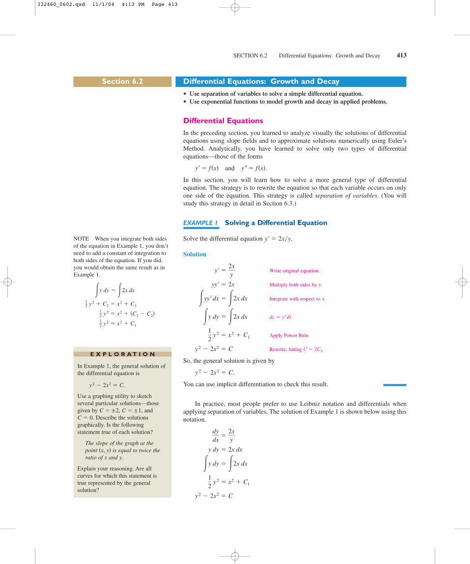
SECTION 6.2 Differential Equations: Growth and Decay 413

Section 6.2 Differential Equations: Growth and Decay

• Use separation of variables to solve a simple differential equation.• Use exponential functions to model growth and decay in applied problems.

Differential Equations

In the preceding section, you learned to analyze visually the solutions of differentialequations using slope fields and to approximate solutions numerically using Euler’sMethod. Analytically, you have learned to solve only two types of differentialequations—those of the forms

and

In this section, you will learn how to solve a more general type of differentialequation. The strategy is to rewrite the equation so that each variable occurs on onlyone side of the equation. This strategy is called separation of variables. (You willstudy this strategy in detail in Section 6.3.)

EXAMPLE 1 Solving a Differential Equation

Solve the differential equation

Solution

Write original equation.

Multiply both sides by

Integrate with respect to

Apply Power Rule.

Rewrite, letting

So, the general solution is given by

You can use implicit differentiation to check this result.

In practice, most people prefer to use Leibniz notation and differentials whenapplying separation of variables. The solution of Example 1 is shown below using thisnotation.

y2 � 2x2 � C

12

y2 � x2 � C1

�y dy � �2x dx

y dy � 2x dx

dydx

�2xy

y2 � 2x2 � C.

C � 2C1. y2 � 2x2 � C

12

y2 � x2 � C1

dy � y� dx �y dy � �2x dx

x. �yy� dx � �2x dx

y. yy� � 2x

y� �2xy

y� � 2x�y.

y� � f�x�.y� � f�x�

NOTE When you integrate both sidesof the equation in Example 1, you don’tneed to add a constant of integration toboth sides of the equation. If you did,you would obtain the same result as inExample 1.

12 y2 � x2 � C1

12 y2 � x2 � �C3 � C2� 12 y2 � C2 � x2 � C3

�y dy � �2x dx

E X P L O R A T I O N

In Example 1, the general solution ofthe differential equation is

Use a graphing utility to sketchseveral particular solutions—thosegiven by and

Describe the solutionsgraphically. Is the followingstatement true of each solution?

The slope of the graph at the point is equal to twice theratio of and

Explain your reasoning. Are allcurves for which this statement istrue represented by the generalsolution?

y.x�x, y�

C � 0.C � ±1,C � ±2,

y 2 � 2x2 � C.

332460_0602.qxd 11/1/04 4:13 PM Page 413

414 CHAPTER 6 Differential Equations

Growth and Decay Models

In many applications, the rate of change of a variable is proportional to the value ofIf is a function of time the proportion can be written as shown.

Rate of change of is proportional to

The general solution of this differential equation is given in the following theorem.

Proof

Write original equation.

Separate variables.

Integrate with respect to

Find antiderivative of each side.

Solve for

Let

So, all solutions of are of the form

EXAMPLE 2 Using an Exponential Growth Model

The rate of change of is proportional to When When What is the value of when

Solution Because you know that and are related by the equationYou can find the values of the constants and by applying the initial

conditions.

When

When

So, the model is When the value of is (see Figure 6.8).

2e0.3466�3� � 5.657yt � 3,y � 2e0.3466t.

t � 2, y � 4.k �12

ln 2 � 0.34664 � 2e2k

t � 0, y � 2.C � 22 � Ce0

kCy � Cekt.tyy� � ky,

t � 3?yy � 4.t � 2,y � 2.t � 0,y.y

y � Cekt.y� � ky

C � eC1. y � Cekt

y. y � ekteC1

ln y � kt � C1

dy � y� dt �1y dy � �k dt

t. �y�y

dt � �k dt

y�y

� k

y� � ky

dydt

� ky

y.y

t,yy.y

t1

1

2

2

3

3

4

4

5

6

7

(0, 2)

(2, 4)

(3, 5.657)

y = 2e0.3466t

y

If the rate of change of is proportional tothen follows an exponential model.

Figure 6.8yy,

y

THEOREM 6.1 Exponential Growth and Decay Model

If is a differentiable function of such that and for someconstant then

is the initial value of and is the proportionality constant. Exponentialgrowth occurs when and exponential decay occurs when k < 0.k > 0,

ky,C

y � Cekt.

k,y� � ky,y > 0ty

STUDY TIP Using logarithmic properties,note that the value of in Example 2 canalso be written as So, the modelbecomes which can then berewritten as y � 2��2�t

.y � 2e�ln�2�t,

ln��2�.k

NOTE Differentiate the functionwith respect to and verify

that y� � ky.t,y � Cekt

332460_0602.qxd 11/1/04 4:13 PM Page 414

SECTION 6.2 Differential Equations: Growth and Decay 415

Radioactive decay is measured in terms of half-life—the number of yearsrequired for half of the atoms in a sample of radioactive material to decay. Thehalf-lives of some common radioactive isotopes are shown below.

Uranium 4,470,000,000 years

Plutonium 24,100 years

Carbon 5715 years

Radium 1599 years

Einsteinium 276 days

Nobelium 25 seconds

EXAMPLE 3 Radioactive Decay

Suppose that 10 grams of the plutonium isotope Pu-239 was released in the Chernobylnuclear accident. How long will it take for the 10 grams to decay to 1 gram?

Solution Let represent the mass (in grams) of the plutonium. Because the rate ofdecay is proportional to you know that

where is the time in years. To find the values of the constants and apply the initial conditions. Using the fact that when you can write

which implies that Next, using the fact that when you canwrite

So, the model is

Half-life model

To find the time it would take for 10 grams to decay to 1 gram, you can solve for inthe equation

The solution is approximately 80,059 years.

From Example 3, notice that in an exponential growth or decay problem, it is easyto solve for when you are given the value of at The next exampledemonstrates a procedure for solving for and when you do not know the value of

at t � 0.ykC

t � 0.yC

1 � 10e�0.000028761t.

t

y � 10e�0.000028761t.

�0.000028761 � k.

1

24,100 ln

12

� k

12

� e24,100k

5 � 10ek�24,100�

t � 24,100,y � 5C � 10.

10 � Cek�0� � Ce0

t � 0,y � 10k,Ct

y � Cekt

y,y

�257No��254Es�

�226Ra��14C�

�239Pu�� 238U�

TECHNOLOGY Most graphing utilities have curve-fitting capabilities that canbe used to find models that represent data. Use the exponential regression feature ofa graphing utility and the information in Example 2 to find a model for the data.How does your model compare with the given model?

NOTE The exponential decay modelin Example 3 could also be writtenas This model is mucheasier to derive, but for some applicationsit is not as convenient to use.

y � 10�12�t�24,100.

Serg

ei S

upin

sky/

AFP

/Get

ty I

mag

es

332460_0602.qxd 11/1/04 4:13 PM Page 415

416 CHAPTER 6 Differential Equations

EXAMPLE 4 Population Growth

Suppose an experimental population of fruit flies increases according to the law ofexponential growth. There were 100 flies after the second day of the experiment and300 flies after the fourth day. Approximately how many flies were in the original population?

Solution Let be the number of flies at time where is measured in days.Because when and when you can write

and

From the first equation, you know that Substituting this value into thesecond equation produces the following.

So, the exponential growth model is

To solve for reapply the condition when and obtain

So, the original population (when ) consisted of approximately flies, as shown in Figure 6.9.

EXAMPLE 5 Declining Sales

Four months after it stops advertising, a manufacturing company notices that its saleshave dropped from 100,000 units per month to 80,000 units per month. If the sales follow an exponential pattern of decline, what will they be after another 2 months?

Solution Use the exponential decay model where is measured in months.From the initial condition you know that Moreover, because

when you have

So, after 2 more months you can expect the monthly sales rate to be

See Figure 6.10.

� 71,500 units.

y � 100,000e�0.0558�6�

�t � 6�,

�0.0558 � k.

ln�0.8� � 4k

0.8 � e4k

80,000 � 100,000e4k

t � 4,y � 80,000C � 100,000.�t � 0�,

ty � Cekt,

y � C � 33t � 0

C � 100e�1.0986 � 33.

100 � Ce0.5493�2�

t � 2y � 100C,

y � Ce0.5493t.

0.5493 � k

12

ln 3 � k

ln 3 � 2k

300 � 100e2k

300 � 100e�2ke4k

C � 100e�2k.

300 � Ce4k.100 � Ce2k

t � 4,y � 300t � 2y � 100tt,y � Cekt

t1 2 3 4

Num

ber

of f

ruit

flie

s

Time (in days)

(4, 300)

(2, 100)

(0, 33)255075

100125150175200225250275300

y = 33e0.5493t

y

Figure 6.9

t1 2 3 4 5 6 7 8

Uni

ts s

old

(in

thou

sand

s)

Time (in months)

(0, 100,000)

(4, 80,000)

(6, 71,500)

20

30

40

10

50

60

70

80

90

100

y = 100,000e−0.0558t

y

Figure 6.10

332460_0602.qxd 11/1/04 4:13 PM Page 416

SECTION 6.2 Differential Equations: Growth and Decay 417

In Examples 2 through 5, you did not actually have to solve the differentialequation

(This was done once in the proof of Theorem 6.1.) The next example demonstrates aproblem whose solution involves the separation of variables technique. The exampleconcerns Newton’s Law of Cooling, which states that the rate of change in thetemperature of an object is proportional to the difference between the object’s temperature and the temperature of the surrounding medium.

EXAMPLE 6 Newton’s Law of Cooling

Let represent the temperature of an object in a room whose temperature iskept at a constant If the object cools from to in 10 minutes, how muchlonger will it take for its temperature to decrease to

Solution From Newton’s Law of Cooling, you know that the rate of change in isproportional to the difference between and 60. This can be written as

To solve this differential equation, use separation of variables, as shown.

Differential equation

Separate variables.

Integrate each side.

Find antiderivative of each side.

Because and you can omit the absolute value signs.Using exponential notation, you have

Using when you obtain which impliesthat Because when

So, the model is

Cooling model

and finally, when you obtain

So, it will require about 14.09 minutes for the object to cool to a temperature of(see Figure 6.11).80�

more

t � 24.09 minutes.

ln 12 � �0.02877t

12 � e�0.02877t

20 � 40e�0.02877t

80 � 60 � 40e�0.02877t

y � 80,

y � 60 � 40e�0.02877t

k �110 ln 34 � �0.02877.

30 � 40e10k

90 � 60 � 40ek�10�

t � 10,y � 90C � 40.100 � 60 � Cek�0� � 60 � C,t � 0,y � 100

C � eC1y � 60 � Cekt.y � 60 � ekt�C1

�y � 60� � y � 60,y > 60,

ln�y � 60� � kt � C1

� 1y � 60

dy � �k dt

� 1y � 60 dy � k dt

dydt

� k�y � 60�

80 ≤ y ≤ 100.y� � k� y � 60�,

yy

80�?90�100�60�.

�in �F�y

y� � ky.

t

Tem

pera

ture

(in

°F)

140

120

100

80

60

40

20

5 10 15 20 25

(0, 100)

(10, 90)(24.09, 80)

y = 60 + 40e−0.02877t

Time (in minutes)

y

Figure 6.11

332460_0602.qxd 11/1/04 4:13 PM Page 417

418 CHAPTER 6 Differential Equations

In Exercises 1–10, solve the differential equation.

1. 2.

3. 4.

5. 6.

7. 8.

9. 10.

In Exercises 11–14, write and solve the differential equationthat models the verbal statement.

11. The rate of change of with respect to is inversely propor-tional to the square of

12. The rate of change of with respect to is proportional to

13. The rate of change of with respect to is proportional to

14. The rate of change of with respect to varies jointly as and

Slope Fields In Exercises 15 and 16, a differential equation, apoint, and a slope field are given. (a) Sketch two approximatesolutions of the differential equation on the slope field, one ofwhich passes through the given point. (b) Use integration to findthe particular solution of the differential equation and use agraphing utility to graph the solution. Compare the result withthe sketch in part (a). To print an enlarged copy of the graph, goto the website www.mathgraphs.com.

15. 16.

In Exercises 17–20, find the function passing throughthe point with the given first derivative. Use a graphingutility to graph the solution.

17. 18.

19. 20.

In Exercises 21–24, write and solve the differential equationthat models the verbal statement. Evaluate the solution at thespecified value of the independent variable.

21. The rate of change of is proportional to When and when What is the value of when

22. The rate of change of is proportional to When and when What is the value of

when

23. The rate of change of is proportional to When and when What is the value of

when

24. The rate of change of is proportional to When and when What is the value of

when

In Exercises 25–28, find the exponential function thatpasses through the two given points.

25. 26.

27. 28.

t1 2 3 4 5

5

4

3

2

1 3, 12( )

(4, 5)

y

t1 2 3 4 5

5

4

3

2

1

(5, 5)

(1, 1)

y

t1 2 3 4 5

4

3

2

1 5, 12( )

(0, 4)

y

t1 2 3 4 5

5

4

3

2

10, 1

2( )

(5, 5)

y

y � Cekt

t � 5?PP � 4750.t � 1,P � 5000

t � 0,P.P

t � 6?VV � 12,500.t � 4,V � 20,000

t � 0,V.V

t � 4?NN � 400.t � 1,N � 250

t � 0,N.N

x � 6?yy � 10.x � 3,y � 4x � 0,y.y

dydt

�34

ydydt

� �12

y

dydt

� �34

�tdydt

�12

t

0, 10�y � f t�

x

4

−4

−4 4

y

x−5 −1

9

5

y

�0, 12�dydx

� xy,�0, 0�dydx

� x�6 � y�,

L � y.xxy

250 � s.sN

10 � t.tP

t.tQ

xy � y� � 100x�1 � x2�y� � 2xy � 0

y� � x�1 � y�y� � �x y

y� ��x3y

y� �5xy

dydx

� 4 � ydydx

� y � 2

dydx

� 4 � xdydx

� x � 2

E x e r c i s e s f o r S e c t i o n 6 . 2 See www.CalcChat.com for worked-out solutions to odd-numbered exercises.

Writing About Concepts29. Describe what the values of and represent in the expo-

nential growth and decay model,

30. Give the differential equation that models exponentialgrowth and decay.

In Exercises 31 and 32, determine the quadrants in whichthe solution of the differential equation is an increasingfunction. Explain. (Do not solve the differential equation.)

31. 32.dydx

�12

x2ydydx

�12

xy

y � Cekt.kC

332460_0602.qxd 11/1/04 4:13 PM Page 418

SECTION 6.2 Differential Equations: Growth and Decay 419

Radioactive Decay In Exercises 33–40, complete the table forthe radioactive isotope.

Half-Life

33. 1599 10 g

34. 1599 1.5 g

35. 1599 0.5 g

36. 5715 2 g

37. 5715 5 g

38. 5715 3.2 g

39. 24,100 2.1 g

40. 24,100 0.4 g

41. Radioactive Decay Radioactive radium has a half-life ofapproximately 1599 years. What percent of a given amountremains after 100 years?

42. Carbon Dating Carbon-14 dating assumes that the carbondioxide on Earth today has the same radioactive content as itdid centuries ago. If this is true, the amount of absorbed bya tree that grew several centuries ago should be the same as theamount of absorbed by a tree growing today. A piece ofancient charcoal contains only 15% as much of the radioactivecarbon as a piece of modern charcoal. How long ago was thetree burned to make the ancient charcoal? (The half-life of is 5715 years.)

Compound Interest In Exercises 43–48, complete the table fora savings account in which interest is compounded continuously.

43. $1000 6%

44. $20,000

45. $750

46. $10,000 5 yr

47. $500 $1292.85

48. $2000 $5436.56

Compound Interest In Exercises 49–52, find the principal that must be invested at rate compounded monthly, so that$500,000 will be available for retirement in years.

49. 50.

51. 52.

Compound Interest In Exercises 53–56, find the time necessaryfor $1000 to double if it is invested at a rate of compounded (a)annually, (b) monthly, (c) daily, and (d) continuously.

53. 54.

55. 56.

Population In Exercises 57– 60, the population (in millions) ofa country in 2001 and the expected continuous annual rate ofchange of the population for the years 2000 through 2010 aregiven. (Source: U.S. Census Bureau, International Data Base)

(a) Find the exponential growth model for the popu-lation by letting correspond to 2000.

(b) Use the model to predict the population of the country in2015.

(c) Discuss the relationship between the sign of and thechange in population for the country.

57. Bulgaria 7.7

58. Cambodia 12.7 0.018

59. Jordan 5.2 0.026

60. Lithuania 3.6

61. Modeling Data One hundred bacteria are started in a cultureand the number of bacteria is counted each hour for 5 hours.The results are shown in the table, where is the time in hours.

(a) Use the regression capabilities of a graphing utility to findan exponential model for the data.

(b) Use the model to estimate the time required for the popula-tion to quadruple in size.

62. Bacteria Growth The number of bacteria in a culture isincreasing according to the law of exponential growth. Thereare 125 bacteria in the culture after 2 hours and 350 bacteriaafter 4 hours.

(a) Find the initial population.

(b) Write an exponential growth model for the bacteria popu-lation. Let represent time in hours.

(c) Use the model to determine the number of bacteria after8 hours.

(d) After how many hours will the bacteria count be 25,000?

63. Learning Curve The management at a certain factory hasfound that a worker can produce at most 30 units in a day. Thelearning curve for the number of units produced per day aftera new employee has worked days is After 20days on the job, a particular worker produces 19 units.

(a) Find the learning curve for this worker.

(b) How many days should pass before this worker is producing25 units per day?

64. Learning Curve If in Exercise 63 management requires anew employee to produce at least 20 units per day after 30 dayson the job, find (a) the learning curve that describes thisminimum requirement and (b) the number of days before aminimal achiever is producing 25 units per day.

N � 30�1 � ekt�.tN

t

tN

�0.002

�0.009

k 2001 PopulationCountry

k

t � 0P � Cekt

k

r � 5.5%r � 8.5%

r � 6%r � 7%

r

t � 25r � 9%,t � 35r � 8%,

t � 40r � 6%,t � 20r � 712%,

tr,

P

7 34 yr

5 12%

10 Years DoubleRate InvestmentAmount AfterTime toAnnualInitial

14C

14C

14C

239Pu

239Pu

14C

14C

14C

226Ra

226Ra

226Ra

10,000 Years1000 YearsQuantity�in years�IsotopeAfterAfterInitialAmountAmount

0 1 2 3 4 5

100 126 151 198 243 297N

t

332460_0602.qxd 11/1/04 4:13 PM Page 419

420 CHAPTER 6 Differential Equations

65. Modeling Data The table shows the population (inmillions) of the United States from 1960 to 2000. (Source:U.S. Census Bureau)

(a) Use the 1960 and 1970 data to find an exponential modelfor the data. Let represent 1960.

(b) Use a graphing utility to find an exponential model forthe data. Let represent 1960.

(c) Use a graphing utility to plot the data and graph bothmodels in the same viewing window. Compare the actualdata with the predictions. Which model better fits the data?

(d) Estimate when the population will be 320 million.

66. Modeling Data The table shows the net receipts and theamounts required to service the national debt (interest onTreasury debt securities) of the United States from 1992through 2001. The monetary amounts are given in billions ofdollars. (Source: U.S. Office of Management and Budget)

(a) Use the regression capabilities of a graphing utility to findan exponential model for the receipts and a quartic model

for the amount required to service the debt. Let representthe time in years, with corresponding to 1992.

(b) Use a graphing utility to plot the points corresponding to thereceipts, and graph the corresponding model. Based on themodel, what is the continuous rate of growth of the receipts?

(c) Use a graphing utility to plot the points corresponding tothe amount required to service the debt, and graph thequartic model.

(d) Find a function that approximates the percent of thereceipts that is required to service the national debt. Use agraphing utility to graph this function.

67. Sound Intensity The level of sound (in decibels), with anintensity of is

where is an intensity of watts per square centimeter,corresponding roughly to the faintest sound that can be heard.Determine for the following.

(a) watts per square centimeter (whisper)

(b) watts per square centimeter (busy street corner)

(c) watts per square centimeter (air hammer)

(d) watts per square centimeter (threshold of pain)

68. Noise Level With the installation of noise suppressionmaterials, the noise level in an auditorium was reduced from93 to 80 decibels. Use the function in Exercise 67 to find thepercent decrease in the intensity level of the noise as a result ofthe installation of these materials.

69. Forestry The value of a tract of timber is

where is the time in years, with corresponding to 1998.If money earns interest continuously at 10%, the present valueof the timber at any time is Find the year inwhich the timber should be harvested to maximize the presentvalue function.

70. Earthquake Intensity On the Richter scale, the magnitude of an earthquake of intensity is

where is the minimum intensity used for comparison.Assume that

(a) Find the intensity of the 1906 San Francisco earthquake

(b) Find the factor by which the intensity is increased if theRichter scale measurement is doubled.

(c) Find

71. Newton’s Law of Cooling When an object is removed froma furnace and placed in an environment with a constanttemperature of its core temperature is F. One hourafter it is removed, the core temperature is F. Find thecore temperature 5 hours after the object is removed from thefurnace.

72. Newton’s Law of Cooling A container of hot liquid is placedin a freezer that is kept at a constant temperature of Theinitial temperature of the liquid is After 5 minutes, theliquid’s temperature is How much longer will it take forits temperature to decrease to

True or False? In Exercises 73–76, determine whether thestatement is true or false. If it is false, explain why or give anexample that shows it is false.

73. In exponential growth, the rate of growth is constant.

74. In linear growth, the rate of growth is constant.

75. If prices are rising at a rate of 0.5% per month, then they arerising at a rate of 6% per year.

76. The differential equation modeling exponential growth iswhere is a constant.kdy�dx � ky,

30�F?60�F.

160�F.20�F.

1120�1500�80�F,

dR�dI.

�R � 8.3�.

I0 � 1.I0

R �ln I � ln I0

ln 10

IR

A�t� � V�t�e�0.10t.t

t � 0t

V�t� � 100,000e0.8�t

I � 10�4

I � 10�6.5

I � 10�9

I � 10�14

��I�

10�16I0

��I� � 10 log10 II0

I�

P�t�

t � 2tI

R

t � 0P2

t � 0P1

P

Year 1992 1993 1994 1995 1996

Receipts 1091.3 1154.4 1258.6 1351.8 1453.1

Interest 292.3 292.5 296.3 332.4 343.9

Year 1997 1998 1999 2000 2001

Receipts 1579.3 1721.8 1827.5 2025.2 1991.2

Interest 355.8 363.8 353.5 361.9 359.5

Year 1960 1970 1980 1990 2000

Population, P 181 205 228 250 282

332460_0602.qxd 11/1/04 4:13 PM Page 420