Section 4

Parameterization of important atmospheric and surface processes,

effects of different parameterizations

Numerical Simulation of Heavy Snowfall and the Potential Role of Ice Nuclei in Cloud Formation and Precipitation Development

Kentaro Araki and Masataka Murakami Meteorological Research Institute, Tsukuba, Japan

e-mail: araki@mri-jma.go.jp 1. Introduction

A heavy snowfall event occurred in the Kanto region from 14 to 15 February 2014, when a winter extratropical cyclone rapidly developed along the south coast of Japan. The snow depth exceeded the historical record in the region, and the event caused many losses of human life. Accurate forecast of such heavy snowfall events is highly required but remains challenging because the precipitation system deeply involves complicated processes of synoptic- and meso-scale dynamics, boundary layer, cloud microphysics, and diabatic process due to phase changes of cloud and precipitation particles. In terms of cloud microphysics, understanding of the aerosol indirect effect by ice nuclei is required. In order to examine the characteristics of cloud microphysics and potential role of ice nuclei in cloud formation and precipitation development during the event, we performed numerical experiments with a horizontal grid spacing of 1.5 km using the Japan Meteorological Agency (JMA) non-hydrostatic model (NHM; Saito et al. 2006) with bulk cloud microphysics scheme. The initial and boundary conditions were provided from 3-hourly JMA mesoscale analysis and the model domain covered the central part of Japan Island, including the Kanto region. The model was run for 33 hours from 0300 Japan Standard Time (JST; JST = UTC + 9 h) on 14 February 2014.

2. Microphysical structures in precipitating clouds and the impact of ice nucleiThe snow depth observations provided by many national organizations and local governments revealed the

detailed distribution of snow depth, where the 33-hour accumulated snowfall exceeded 1 m in the mountain areas (Fig. 1). The control experiment successfully reproduced the distribution of snowfall (Fig. 4). By comparisons with the surface observation, wind profiler, and liquid water path retrieved from ground-based microwave radiometer data in these regions, simulated dynamic and thermodynamic environment and cloud microphysical properties reasonably agreed with observations (not shown). A coastal front was formed in the south of the Kanto region, and the feature of the cold air damming as U-shaped contour of sea level pressure was found in the Kanto region (Fig. 2). The coastal front got distinct as the north-south gradient of sea level pressure increased (Fig. 3a), and diabatic cooling by sublimation/evaporation/melting of precipitation particles in lower troposphere also contributed to the formation and maintenance of coastal front and cold air damming. A distinct meso-scale vortex, usually called zipper low, was formed on the front before the passage of the cyclone (Fig. 2), and would play a role in the maintenance of the coastal front. Warm and moist southeasterly wind flowed on the front, and brought a large amount of water vapor (Fig. 3b), resulting in the heavy snowfall in the Kanto region. The synoptic-scale features of upper-level coupled jet structure, causing acceleration of low-level ageostrophic flows and enhancement of the coastal front, were also found by JMA mesoscale analysis (not shown), which was quite similar to the situation of heavy snowfall events in the east coast of the United States (Uccellini and Kocin 1987).

Clouds composed of solid cloud and precipitation particles were simulated in the 8–12 and 2–4 km layers, and the latter cloud layers were formed both above the surface of the coastal front and on the windward side of the mountains (Fig. 5). Number density of snow was large at a layer between 5 and 10 km altitude and another layer

Figure 3. (a) Time-range cross section of simulated temperature at 20 m above the surface (shade) and sea level pressure (contour) along the solid line AB in Fig. 2. (b) Time-height cross section of water vapor flux (shade) and temperature (contour) at the Ome city. Barbs indicate horizontal wind.

Figure 1. Horizontal distribution of 33-hour accumulated snowfall (cm) from 0300 JST on 14 Febr to 1200 JST on 15 Febr obtained from the sum of the differences of 1-hourly snow depth observations.

Figure 2. Horizontal distribution of simulated temperature (shade) and sea level pressure (contour) converted from pressure at 20 m above the surface at 1930 JST on 14 Febr. Vectors indicate horizontal wind at the same level.

between 2 and 4 km altitude, and mixing ratio of snow was large below about 8 km altitude. In this case, there were two layers of stratiform ice clouds to the north of the coastal front and on the windward side of the mountains, and the other low-level clouds were also formed by orographically-induced updraft in the mountain regions, resulting in the seeder-feeder mechanism which contributed to the increase of snowfall amount (Houze 2012). On the other hand, the 33-hour accumulated precipitation by graupel reached 20 mm in some parts of the Kanto region (Fig. 4), which was formed by riming growth during the passage of the cyclone over the Kanto plain, where sufficient water vapor supply and super-cooled cloud water locally existed near the center of the cyclone in low-level troposphere.

In order to investigate the effect of ice nuclei (number of cloud ice) on cloud formation and precipitation development, sensitivity experiments were performed by changing coefficients in the formulas of deposition/condensation-freezing-mode ice nucleation (Meyers 1992) and immersion-freezing-mode ice nucleation (Bigg 1955) by factors of 0.1 (IN01) and 10 (IN10). As a result, there were differences of accumulated snow precipitation by of –5 mm in water equivalent for IN01 case and +5 mm for IN10 case as compared with INdef case on the windward side of mountain regions. On the leeward side of mountain regions, there were opposite differences of accumulated precipitation by snow of +5 mm for IN01 and –10 mm for IN10. The accumulated rainfall increased more than 15 mm for IN01 and decreased more than 20 mm for IN10 on the coastal region, whereas the similar amount of rainfall decrease/increase was found off shore. Since there were sufficient water vapor supply below about 6 km altitude (Fig. 3b) and rather low number concentrations of snow for INdef, the conversion of cloud ice into snow and consequent snowfall amount decreased in IN01 and increased in IN10, respectively (Fig. 5). For IN10 case, large number of cloud ice were converted into snow on the windward side of the coastal front over the ocean, and amount of rain produced from melted snow particles increased off shore and decreased on shore and vice versa for IN01 case. The similar contrast was produced on the windward and leeward of low-level orographic clouds; the increase and decrease of snowfall amount on the leeward side of mountains in IN01 and IN10, respectively. This contrast of low-level orographic clouds would be caused by the differences of water vapor supply which increased in IN01 and decreased in IN10 on the windward side of mountains, respectively. On the other hand, precipitation amount by graupel decreased by about 5 mm for IN01 case and increased by more than 10 mm for IN10 case in a part of the Kanto region during the passage of the cyclone. Since there were a large amount of low-level water vapor and supercooled cloud water fluxes as compared with number concentration of snow for INdef case, the increase in snow number concentrations due to enhanced ice nucleation may lead to the increase in graupel precipitation. 3. Conclusions and remarks

The synoptic, mesoscale, and cloud microphysical factors causing a heavy snowfall were investigated through a case study. It’s found that the maintenance of the coastal front and the seeder-feeder mechanism were important in the increase of snowfall amount. The result also suggests that concentrations of ice nuclei (cloud ice) considerably affect snowfall amount and its distribution. It’s required to develop a numerical model which properly handles the aerosol effects on the cloud formation and precipitation development.

References: Houze, R. A., 2012: Orographic effects on precipitating clouds. Rev. Geophys., 50, RG1001, doi:10.1029/2011RG000365. Saito, K., T. Fujita, Y. Yamada, J. Ishida, Y. Kumagai, K. Aranami, S. Ohmori, R. Nagasawa, S. Kumagai, C. Muroi, T. Kato, H. Eito,

and Y. Yamazaki, 2006: The operational JMA nonhydrostatic mesoscale model. Mon. Wea. Rev., 134, 1266–1298. Uccellini, L. W., and P. J. Kocin, 1987: The interaction of jet streak circulations during heavy snow events along the east coast of the

United States. Wea. Forecasting, 2, 289–308.

Figure 5. Vertical cross sections of number densities of cloud ice and snow, mixing ratio of snow, and water vapor flux along the broken line CD in Fig. 2 at 0000 JST on 15.

Figure 4. Horizontal distributions of 33-hour accumulated precipitation (mm) from 0300 JST on 14 to 1200 JST on 15 by snow, graupel, and rain simulated by INdef (left panels). Horizontal distributions of the difference between IN01/IN10 and INdef (center/right panels).

Improvement of cumulus convection and planetary boundary layer parameterizations in the NCEP GFS 

Jongil Han NOAA/NWS/NCEP Environmental Modeling Center, College Park, MD, USA,

e-mail: Jongil.Han@noaa.gov

A new shallow cumulus convection scheme has been implemented into the NCEP Global Forecast  System  (GFS;  2010), which  employs  a mass  flux parameterization  replacing  the old turbulent diffusion‐based approach and helps not to destroy stratocumulus clouds off the West coasts  of  South  America  and  Africa  as  the  old  scheme  does.  The  deep  cumulus  convection scheme  was  revised  to  make  cumulus  convection  stronger  and  deeper  to  deplete  more instability  in the atmospheric column and result  in the suppression of the excessive grid‐scale precipitation  (2010).  The  planetary  boundary  layer  (PBL)  scheme  was  revised  to  enhance turbulence diffusion in stratocumulus regions (2010), which helps prevent too much low cloud from forming. 

Recently,  a  hybrid  eddy‐diffusivity  mass‐flux  (EDMF)  PBL  scheme  with  dissipative heating and modified stable PBL mixing has been implemented into the NCEP GFS (2015). With the EDMF PBL scheme, where the nonlocal transport by  large turbulent eddies  is represented by a mass‐flux (MF) scheme and the local transport by small eddies is represented by an eddy‐diffusivity  (ED)  scheme,  the daytime PBL growth was  improved.  In order not  to degrade  the forecast skill in the tropical ocean where strongly unstable PBLs are rarely found, a hybrid EDMF PBL  scheme  has  been  adopted,  where  the  EDMF  scheme  is  applied  only  for  the  strongly unstable PBL, while the old GFS eddy‐diffusivity counter‐gradient (EDCG) scheme is used for the weakly unstable PBL. For the vertical momentum mixing, the MF scheme is modified to include the  effect  of  the  updraft‐induced  pressure  gradient  force.  To  enhance  a  too weak  vertical turbulent mixing for weakly and moderately stable conditions, the current local scheme in the stable boundary  layer  is modified  to use an ED profile method. On  the other hand,  the drag coefficient over sea was reduced  in high wind speeds to  increase hurricane  intensity which  is generally weaker than the observation in the GFS due to coarse resolution. 

Necessity of parameterizations for convective initiationin high resolution cloud-permitting models

TABITO HARA

Numerical Prediction Division, Japan Meteorological Agency1-3-4, Ote-machi, Chiyoda-ku, Tokyo 100-8122, Japan

1 IntroductionNWP centers around the world, including the Japan Me-

teorological Agency (JMA), have recently begun operat-ing high resolution cloud-permitting models with horizon-tal grid spacing of around 2-km with no convective pa-rameterizations. JMA’s operational 2-km model, calledthe Local Forecast Model (LFM), has been in operationsince August 2012, with the forecast domain expanded inMay 2013 to cover Japan and the surrounding area. Itsinitial conditions are generated by three-hour data assim-ilation cycles combined with the three-dimensional vari-ational assimilation method and one-hour forecasts fromthe forecasting model. Forecasts are updated every hour.

Higher resolution models are considered capable of re-solving a significant part of vertical transportation of mo-mentum, heat and moisture, which is the main feedbackof convection, in the form of vertical advection with grid-mean vertical velocities, meaning that no convective pa-rameterizations are required. However, verification to ex-amine the performance of JMA’s 2-km operational modelrevealed issues related to convection such as delays in con-vective initiation and excessive intensity of convective ac-tivities.

This report first outlines verification of the operational 2-km model with focus on convective initiation, then dis-cusses possible reasons for the delays in convective initiation. Finally, an attempt to resolve the issues and its outcome are described.2 Delay in convective initiation shown by verification

of the operational modelFigure 1 shows a timeseries representation of the num-

ber of grids in which precipitation exceeding 1 mm/h is observed (red bars) and predicted by the operational model (purple line). The numbers of events are accumulated over several cases in which showers associated with unstably stratified layers occurred. The figure shows that while most events with precipitation exceeding 1 mm/h were observed at 16 JST (Japanese local time), the peak time of current operational predictions delayed by around two hours from the corresponding observation, which means that convection is not initiated at an appropriate time in the current 2-km operational model. Similar tendencies can be also seen in Figure 2 timeseries representation showing the observed and predicted frequencies of precipitation exceeding 10 mm/h.

3 Effects of enhancing the dynamical and boundarylayer scheme

*E-mail: tabito.hara@met.kishou.go.jp

alent to or more enhanced than those of the JMA-NHMwere implemented via use of the “Physics library” (Haraet al. 2012). In particular, the improved Mellor-Yamada-Nakanishi-Niino level 3 model (MYNN3; Nakanishi andNiino (2009)) used as a boundary layer turbulence schemewas refined so that turbulent fluxes and tendencies of prog-nostic variables in the turbulence scheme can be stablysolved, removing temporarily fluctuated, noisy, and over-estimated turbulent fluxes.

In the initial stage of ASUCA development, no convec-tive parameterization was implemented (as with the op-erational model employing JMA-NHM at the time). Forthe delay in convective initiation described in the previ-ous section, ASUCA improved the delay in precipitationpeak as shown by the green line in Figure 1 (although thefrequency shortage at the initiation stage remains unre-solved). This implies that refinement of the dynamical andthe boundary layer scheme is highly related to the timingof convective initiation. However, the delay still has roomfor improvement.

4 Possible cause of convective initiation delayIt is considered that the main feedback of convection

such as vertical transport of momentum, heat and mois-ture can be represented by grid-mean vertical velocity inmodels with a horizontal resolution of a few kilometers orless. However, this does not necessarily mean that all phe-nomena (especially initiating and controlling convection)can be resolved in high resolution models. For example,the forced lifting necessary to initiate convection wouldoften be induced by small scale convergence and smallscale topography variance, but some cases may not be re-solved even if vertical transport is represented. The lackof smaller phenomena related to convective initiation inthe models explains the delay in convective precipitationpeaks predicted by the 2-km operational model and eventhe newer model in comparison with observations.

5 Parameterization for convective initiationAs an attempt, a parameterization to represent convec-

tive initiation was implemented in ASUCA. The parame-terization is based on the existing convective parameteri-zation suggested by Kain and Fritsch (1990) (known as KFscheme), but it has been modified assuming slower con-vective stabilization, implying that tendency from convec-tive processes is much smaller than for the original con-vective parameterization.

The KF convection scheme, which is employed in the5-km operational meso scale model at JMA, diagnoses afinal state in which a certain ratio r of the initial convectiveavailable potential energy (CAPE) is removed for a certainlife time of convection τ :

dCAPE

dt= −(1− r)

CAPEinitial

τ. (1)

Tendencies of prognostic variables ϕ are calculatedusing the difference between the initial and final states

JMA replaced the old non-hydrostatic model (JMA-NHM; Saito et al. (2007)) with a new one called “ASUCA”at the end of January 2015 (Aranami et al. 2015). ASUCAhas been developed as a new dynamical core with higheraccuracy and better computational efficiency on massiveparallel scalar supercomputers. Physical processes equiv-

0

2000

4000

6000

8000

10000

12000

14000

16000

18000

20000

13 14 15 16 17 18 19 20 21

Fre

quen

cy

JST

gauge:2 threshold:1 mean 03initial

observationasuca w/o PI

asuca w/ PILFM

Fig. 1: Timeseries representation of the number of grids at whichprecipitation exceeding 1 mm/h is observed (red bars) and pre-dicted by models (lines). Purple line: the operational model,green and blue lines: ASUCA without / with the parameteri-zation of initiation, respectively

0

1000

2000

3000

4000

5000

6000

13 14 15 16 17 18 19 20 21

Fre

quen

cy

JST

gauge:2 threshold:10 mean 03initial

observationasuca w/o PI

asuca w/ PILFM

Fig. 2: As per Figure 1, but for precipitation exceeding 10mm/h

(ϕinitial and ϕfinal, respectively) :

∂ϕ

∂t=

ϕfinal − ϕinitial

τ. (2)

In the modified scheme to parameterize convective ini-tiation, a longer value of τ is adopted (meaning weakerconvective activity and smaller tendencies from convec-tion) aiming at representing weaker vertical transport andrelease of latent heat in the initial stage of convection. Inaddition, the convection scheme is modified so that finalstates and tendencies are diagnosed at every timestep, asopposed to the fixed-interval evaluation of the original KFscheme (e.g. five minutes). Updating of tendencies at ev-ery timestep makes the modified scheme more sensitive todeveloping convection produced by dynamical processesin models.

If dynamical processes in models do not produce up-draft due to convection even with the realization of an un-stably stratified layer, the parameterization is activated andmodifies layer stratification by weakly transporting heatand moisture vertically and releasing latent heat throughthe phase transition of water, resulting in the production ofa local low pressure area. Once such a local low pressurearea is generated, dynamical processes in models calcu-late convergence into the low pressure area and promotesdevelopment of convection. As it acts very weakly, theparameterization just helps dynamical processes to fosterthe convective system.

The blue lines in Figures 1 and 2 indicate forecast fre-quency from ASUCA with the parameterization to helpinitiation. For levels of precipitation exceeding 1 mm/h(Figure 1), the forecast frequency at 13 JST (usually theinitial stage of convection) is much closer to the obser-vation frequency (but still smaller than the actual obser-vation). The overall temporal evolution of precipitationfrequency is also significantly improved for precipitationexceeding both 1 mm/h and 10 mm/h (Figure 2). The newparameterization is proven to be quite effective in easingconvective initiation delay.

6 DiscussionDevelopment of the proposed parameterization for con-

vective initiation was motivated by recognition that var-ious scales related to convective phenomena are mixed.

While the parameterization currently targets convectiveinitiation which cannot necessarily be resolved even incloud-permitting models with horizontal grid spacing ofa few kilometers, there are other phenomena that cannotbe resolved even if vertical transport by convection is rep-resented. By way of example, entrainment plays an impor-tant role because it controls convective activity by dilutingcumuli. However, its scale may be too small to resolvein cloud-permitting models. This may be one reason whyoverly strong vertical velocity is sometimes predicted inhigh resolution models when no convective schemes areadopted. To represent the effect of entrainment-relatedweakening of convective activity (and secure computa-tional stability) in ASUCA, vertical velocity is suppressedby adding an extra term to its tendency. However, evalua-tion of this extra term has no robust physical basis becauseit depends only on the CFL conditions and involves noconsideration for the physical processes of entrainment.More physical methods of estimating effects of entrain-ment are necessary for further model improvement.

The proposed parameterization for convective initiationis just one example, and it is challenging to treat resolvedand unresolved phenomena at the same time. It is exactlyrelated to “Grey Zone” problem.

ReferencesAranami, K., T. Hara, Y. Ikuta, K. Kawano, K. Matsubayashi,

H. Kusabiraki, T. Ito, T. Egawa, K. Yamashita, Y. Ota,Y. Ishikawa, T. Fujita, and J. Ishida, 2015: A new oper-ational regional model for convection-permitting numericalweather prediction at JMA. CAS/JSC WGNE Res. Activ. At-mos. Oceanic Modell., 45, submitted.

Hara, T., K. Kawano, K. Aranami, Y. Kitamura, M. Sakamoto,H. Kusabiraki, C. Muroi, and J. Ishida, 2012: Development ofthe Physics Library and its application to ASUCA. CAS/JSCWGNE Res. Activ. Atmos. Oceanic Modell., 42, 0505–0506.

Kain, J. S. and J. M. Fritsch, 1990: A One-Dimensional Entrain-ing/Detraining Plume Model and Its Application in Convec-tive Parameterization. J. Atmos. Sci., 47, 2784–2802.

Nakanishi, M. and H. Niino, 2009: Development of an ImprovedTurbulence Closure Model for the Atmospheric BoundaryLayer. J. Meteor. Soc. Japan, 87, 895–912.

Saito, K., J. Ishida, K. Aranami, T. Hara, T. Segawa, M. Narita,and Y. Honda, 2007: Nonhydrostatic Atmospheric Modelsand Operational Development at JMA. J. Meteor. Soc. Japan,85B, 271–304.

Factors of model underestimation of snow fall over the Japan-Sea coastal areas in middle Japan: Comparison with observed precipitation particles

Teruyuki Kato1, Hiroki Motoyoshi2, Yoshinori Yamada1, Akihiko Hashimoto1, Sento Nakai2, Masaaki Ishizaka2 1Meteorological Research Institute/Japan Meteorological Agency (Email: tkato@mri-jma.go.jp)

2Snow and Ice Research Center/National Research Institute for Earth Science and Disaster Prevention

1. IntroductionPolar air outbreak from the Eurasia Continent often brings heavy snow fall over the Japan-Sea coastal areas during the winter season. The Japan Meteorological Agency (JMA) operational mesoscale model (horizontal resolution: 5 km), however, usually underestimates snow fall amounts over plain areas, while mountainous areas have overestimations. In Snow and Ice Research Center of National Research Institute for Earth Science and Disaster Prevention, located in the plain area (see the location marked by symbol of X in Fig. 2), the size and terminal velocity of precipitation particles have been captured every minute by a charge-coupled device camera and a Parsivel optical disdrometer. Then by using the method of Ishizaka et al. (2013), the main type of solid hydrometeors contributing to precipitation has been identified from the relationship between measured size and fall speed every five minutes (e.g., see Fig. 1a).

In this study, hydrometeor types simulated by JMA nonhydrostatic model (NHM: Saito et al. 2007) with difference resolution are compared with identified observation ones, and the underestimation of snowfall amounts over plain areas is examined.

2. Experimental designsOne-day forecasts from 03 JST (=UTC+ 9hs) 04 January 2013 were conducted using initial and boundary conditions produced from 3-hourly available JMA mesoscale analyses with a horizontal resolution of 5 km. At first a 5km-NHM with a large domain (2500x 2000km) was run, and then for a small domain of 850x550km 2km and 1km-NHMs were run nested within 5km-NHM forecasts. Further, for a domain of 330x250km 500m and 250m-NHMs were run nested within forecasts of 1km-NHM. A bulk-type microphysics parameterization scheme in which two moments are treated only for ice hydrometeors is used for precipitation processes, and the Kain-Fritsch convection parameterization scheme is additionally used only in 5km-NHM. The turbulence closure scheme of Mellor-Yamada-Nakanishi-Niino level-3 (MYNN: Nakanishi and Niino 2006) is used in 5km, 2km, and 1km-NHMs, while Deardroff (DD) scheme (1980) is used in 1km, 500m and 250m-NHMs.

3. Comparison with observationsThe underestimation of snow fall amounts including graupel over plain areas indicated by ellipses in Figs. 2a and 2b is improved using 1km-NHM (Fig. 2d). This improvement is mainly caused by the production of graupel around coastal areas (Fig. 2c), while 5km-NHM hardly produces graupel (not shown) and graupel ratios of 2km-NHM (Fig. 2b) are less 50% of those of 1km-NHM (Fig. 1c). The proportion of graupel in 1km-NHM, however, is considerably smaller in comparison with identified observation types of hydrometeors (Fig. 1a). This small ratio is not improved using 250m-NHM (Fig. 1d). These improvements and resolution dependency agree with Kato (2011, 2012).

4. Effect of terminal velocityIn 5km-NHM, instead of graupel, snow particles could be excessively produced and most of them move to mountainous areas without falling down due to the terrain-induced upward motion (Fig. 3a).

Fig. 1 (a) Identified observation types of hydrometeors between 30 November 2012 and 05 January 2013. Same as (a), but results simulated by (b) 2km, (c) 1km and (d) 250m models during one day from 03 JST January 2013.

To ascertain this hypothesis, a sensitivity experiment in which the terminal velocity of snow on land is replaced with that of graupel was conducted using 5km-NHM. The results (Figs. 2c and 3b) show the improvement of underestimation of snow fall amounts over plain areas, and that of excessively production of snow particles, which suggests that a new parameterization of the production of graupel is necessary for coarse resolution models.

5. Other Impacts on snowfall amountsMuch water cloud is necessary for the production of graupel (i.e. riming process). Since cloud ice hardly exists in warm-rain clouds with the temperature higher than -4C, cloud ice crystal nucleating activity is restricted above -4C to increase cloud water amounts. The results of 2km- and 1km-NHMs, however, showed no improvement for the production of graupel. Another sensitivity

experiment in which the evaporation of graupel is restricted also hardly impacts the graupel fall amounts on the ground, because low-level humidity around coastal areas is high (~80%). On the other hand, the restriction of the evaporation of snow causes the increase of snowfall amounts over the sea and the decrease over plain areas, which agrees with Kato (2011).

References

Ishizaka, M., H. Motoyoshi, S. Nakai, T.

Shiina, T. Kumakura, and K. Muramoto,

2013: J. Meteor. Soc. Japan, 91, 747-762.

Kato, T., 2012: CAS/JSC Research

Activities in Atmospheric and Oceanic

Modeling, 42, 4.09-4.10.

Kato, T., 2011: CAS/JSC Research

Activities in Atmospheric and Oceanic

Modeling, 41, 3.03-3.04.

Saito, K., J. Ishida, K. Aranami, T. Hara,

T. Segawa, M. Nareta, and Y. Honda,

2007: J. Meteor. Soc. Japan, 85B, 271-

304.

Fig. 2 (a) Distribution of 24- hour accumulated Rain- Raingauge analyzed rainfall amounts at 03 JST 05 January 2013. Same as (a), but total precipitation amounts simulated by (b, c) 5km and (e) 1km models with MYNN scheme. (d) Same as (e), but graupel amounts. For (c), the terminal velocity of snow on land was replaced with that of graupel.

Fig. 3 (a) Vertical cross section of 24-hour mean snow mixing ratios on the dashed line in Fig. 2b, simulated by 5km-NHM. Wind vectors show streams projected on the section. (b) Same as (a), but the terminal velocity of snow on land was replaced with that of graupel.

Inner Time Loop Application for Vertical Turbulent Diffusion Processes

Takuya KOMORI Climate Prediction Division, Japan Meteorological Agency, Tokyo, Japan

Email: komori@met.kishou.go.jp

1. INTRODUCTION In operational numerical prediction models, efforts have been made to use a longer time-step as a way of

reducing the computational cost. However, detailed investigation of the Global Spectral Model (GSM) in an

idealized experiment revealed that numerical instability could be occurred in tendencies due to vertical

turbulent diffusion with the over-implicit scheme in certain situations over land, where surface turbulent

fluxes increased rapidly after sunrise and became large. These results suggest that a shorter time-step should

potentially be used in the operational system (JMA 2013). Accordingly, an inner time loop was applied in the

GSM for the calculation of vertical turbulent diffusion processes with a shorter time-step to alleviate

numerical instability. This reduces the computational cost in operational use as compared to that incurred in

the application of a shorter time-step for all processes in the model.

2. INNER TIME LOOP APPLICATION

Using an inner time loop, processes can be calculated with a shorter time-step, t , than the normal

time-step, t , depending on the number of the time loops N : Ntt / . Accordingly, doubling N will halve

the time-step in a process. In this study, an inner time loop was introduced after calculation of fluxes and

tendencies due to short and long waves, thereby enabling skin temperature updating before calling of the

vertical turbulent diffusion scheme (VDF). To maintain interaction between the lowest model level and the

surface via vertical turbulent transport at each inner time-step, calculation of surface turbulent fluxes (SURF)

was also included in the inner time loop. The tendencies of the forecast variable in each inner time loop

were added to update the variable in the previous loop , where is identical to the forecast variable ,

in the normal time-step. All estimated tendencies in the inner time loops were summed up and added to

tendencies due to radiation (RAD), convection (CONV), cloud (CLD), and both orographic and

non-orographic gravity wave drags (GWD) as part of physics processes (PHY) at every normal time-step as

follows:

N

SURFVDF

N

GWDCLDCONVRADPHY tNttttt 1

1

3. EVALUATION

Two experiments (CNTL and TEST) were conducted to evaluate the impact of the inner time loop in

84-hour forecasts. The CNTL experiment was based on the GSM. In the TEST experiment, an inner time

loop with a halved time-step (N = 2) was applied to vertical turbulent diffusion and surface processes.

Figures 1 and 2 respectively show the simulated temperature and moisture tendencies due to physical

processes in pressure-time cross sections at the ARM (Atmospheric Radiation Measurement) SGP (Southern

Great Plains) site. As a general characteristic, no significant difference was seen between CNTL and TEST

around the site. The model-level output in CNTL at each time-step up to the 84-hour forecast with an initial

time of 00 UTC on 4 August 2013 exhibited numerical oscillation with changes in the tendency of the

positive/negative characteristic in turn with each time step in certain situations. Conversely, no numerical

oscillation was observed in TEST, which was characterized by smoothed and increased tendencies.

Performance was verified against wind-profiler observation data distributed via WMO’s global

telecommunication system from near the ARM SGP site. Figure 3 shows pressure-time cross sections of

wind speeds as simulated in the CNTL and TEST experiments, as well as wind-profiler observation data.

During this period, the nocturnal low level jet (NLLJ) was observed over the Great Plains every night. The

wind speeds in TEST were enhanced in association with the potential temperature profiles with decoupling

of the nocturnal stable boundary layer (not shown). This makes the NLLJ representation closer to the

observation in comparison with CNTL, though there is still room for improvement. Accordingly, as well has

helping to alleviate instability, the results of this study also represent a useful step toward better atmospheric representation. Further investigation is needed to explore the sensitivity of land-atmosphere coupling.

N

1N 1

REFERENCE JMA, 2013: Outline of the operational numerical weather prediction at the Japan Meteorological Agency.

Appendix to WMO technical progress report on the global data-processing and forecasting system and numerical weather prediction research. 188pp. Available online: http://www.jma.go.jp/jma/jma-eng/jma-center/nwp/outline2013-nwp/index.htm

Figure 1. Pressure-time cross section of temperature tendency due to physical processes [K/day] for the (a)

CNTL and (b) TEST experiments at the ARM SGP site. Model-level data were output at every time-step up

to the 84-hour forecast with an initial time of 00 UTC on 4 August 2013.

Figure 2. Same as Figure 1, but for moisture tendency due to physical processes [g/kg/day].

Figure 3. Pressure-time cross sections of wind speeds [m/s] for the (a) CNTL experiment, (b) TEST

experiment and (c) wind-profiler observation near the ARM SGP site. In the experiments, model-level data

were output hourly up to the 84-hour forecast with an initial time of 00 UTC on 4 August 2013.

(a) CNTL

(c) OBS (b) TEST

(a) CNTL (b) TEST

(a) CNTL (b) TEST

Toward developing global aerosol modeling and data assimilation capabilities at NOAA/NCEP

for improving weather and air quality forecasts

Sarah Lu (Sarah.Lu@noaa.gov) and Jun Wang (Jun.Wang@noaa.gov) NOAA/NWS/NCEP Environmental Modeling Center, College Park, MD, USA

NCEP recently implemented the NEMS GFS Aerosol Component (NGAC) for global dust forecasts.

With further development, NEMS GFS can be used for modeling and assimilating aerosols and

reactive gases on a global scale. The global modeling/assimilation efforts not only allow aerosol

impacts on weather forecasts and climate predictions to be considered, but also enable NCEP to

provide quality atmospheric constituent products serving a wide-range of stakeholders, such as health

professionals, aviation authorities, policy makers, and solar energy plant managers.

NCEP’s global in-line aerosol forecast system

NASA’s bulk aerosol scheme (an in-line version of the Goddard Chemistry, Aerosol, Radiation,

and Transport model [GOCART], Chin et al., 2002; Colarco et al., 2010) has been incorporated into the

NOAA Environmental Modeling System (NEMS) to establish the first interactive global aerosol

forecasting system, NEMS GFS Aerosol Component (NGAC), at NCEP (Lu et al., 2013). The NGAC

was added to NCEP’s production suite in 2012, providing 120-hour daily global dust forecasts. A major

NGAC upgrade (multi-species forecasts for dust, sea salt, sulfate, and carbonaceous aerosols using near-

real-time satellite-based smoke emissions) is slated for operational implementation in late 2015.

The rationale for developing the global aerosol forecasting capabilities at NOAA includes: (1) to

improve weather forecasts and climate predictions by taking into account aerosol effects on radiation

and clouds; (2) to provide a first step toward aerosol data assimilation and reanalysis; (3) to improve

assimilation of satellite observations by properly accounting for aerosol effects; (4) to provide aerosol

(lateral and upper) boundary conditions for regional air quality predictions; and (5) to produce quality

aerosol information that addresses societal needs and stakeholder requirements, e.g., UV index, ocean

productivity, visibility, air quality, and sea surface temperature retrievals.

Applications of NGAC products

The Consensus International Cooperative for Aerosol Prediction (ICAP) multi-model ensemble

(ICAP-MMES, Sessions et al., 2015) became pseudo-operational in 2014, using four complete aerosol

forecast models from the European Centre for Medium-Range Forecasts (ECMWF), Naval Research

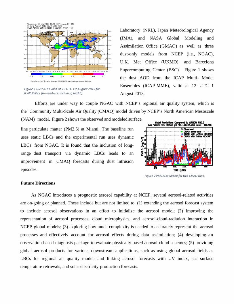
Figure 1 Dust AOD valid at 12 UTC 1st August 2013 for ICAP MMEs (6-members, including NGAC).

Laboratory (NRL), Japan Meteorological Agency

(JMA), and NASA Global Modeling and

Assimilation Office (GMAO) as well as three

dust-only models from NCEP (i.e., NGAC),

U.K. Met Office (UKMO), and Barcelona

Supercomputing Center (BSC). Figure 1 shows

the dust AOD from the ICAP Multi- Model

Ensembles (ICAP-MME), valid at 12 UTC 1

August 2013.

Efforts are under way to couple NGAC with NCEP’s regional air quality system, which is

the Community Multi-Scale Air Quality (CMAQ) model driven by NCEP’s North American Mesoscale

(NAM) model. Figure 2 shows the observed and modeled surface

fine particulate matter (PM2.5) at Miami. The baseline run

uses static LBCs and the experimental run uses dynamic

LBCs from NGAC. It is found that the inclusion of long-

range dust transport via dynamic LBCs leads to an

improvement in CMAQ forecasts during dust intrusion

episodes.

Future Directions

As NGAC introduces a prognostic aerosol capability at NCEP, several aerosol-related activities

are on-going or planned. These include but are not limited to: (1) extending the aerosol forecast system

to include aerosol observations in an effort to initialize the aerosol model; (2) improving the

representation of aerosol processes, cloud microphysics, and aerosol-cloud-radiation interaction in

NCEP global models; (3) exploring how much complexity is needed to accurately represent the aerosol

processes and effectively account for aerosol effects during data assimilation; (4) developing an

observation-based diagnosis package to evaluate physically-based aerosol-cloud schemes; (5) providing

global aerosol products for various downstream applications, such as using global aerosol fields as

LBCs for regional air quality models and linking aerosol forecasts with UV index, sea surface

temperature retrievals, and solar electricity production forecasts.

An improved approximation for the moist-air

entropy potential temperature θs Pascal Marquet

Meteo-France. CNRM/GMAP. Toulouse. France. E-mail: pascal.marquet@meteo.fr

1 Motivations

The moist-air entropy is defined in Marquet (2011,

hereafter M11) by s = sref + cpd ln(θs) in terms of

two constant values (sref , cpd) and a potential entropytemperature denoted by θs. It is shown in M11 thata quantity denoted by (θs)1 plays the role of a leadingorder approximation of θs.

The aim of this note is to demonstrate in a morerigorous way that (θs)1 is indeed the leading order ap-proximation of θs, and to derive a second order ap-proximation which may be used in computations ofvalues, gradients or turbulent fluxes of moist-air en-tropy. Some impacts of this second order approxima-tion are described in this brief version of a note to besubmitted to the QJRMS.

2 Definition of θs and (θs)1

The potential temperature θs is defined in M11 by

θs = (θs)1

(T

Tr

)λ qt( p

pr

)−κ δ qt(rrrv

)γ qt (1+η rv)κ (1+ δ qt)

(1+η rr)κ δ qt

where (θs)1 = θl exp(Λr qt) . (1)

This definition of θs is rather complex, but themore simple quantity (θs)1 was considered in M11as a leading order approximation of θs, where theBetts’ potential temperature is written as θl =θ exp[ − (Lv ql + Ls qi) / (cpd T ) ].

The total water specific content is qt = qv + ql +qi and rv is the water vapour mixing ratio. Otherthermodynamic constants are: Rd ≈ 287 J K−1, Rv ≈461.5 J K−1, cpd ≈ 1005 J K−1, cpv ≈ 1846 J K−1,κ = Rd/cpd ≈ 0.286, λ = cpv/cpd − 1 ≈ 0.838, δ =Rv/Rd−1 ≈ 0.608, η = Rv/Rd ≈ 1.608, , ε = Rd/Rv ≈0.622 and γ = Rv/cpd ≈ 0.46.

The term

Λr = [ (sv)r − (sd)r ] / cpd ≈ 5.87 (2)

depends on reference entropies of dry air and watervapour at Tr = 0 C, denoted by (sd)r = sd(Tr, er) and(sv)r = sv(Tr, pr − er), where er = 6.11 hPa is thesaturating pressure at Tr and pr = 1000 hPa. The tworeference entropies (sv)r ≈ 12673 J K−1 and (sd)r ≈6777 J K−1 are computed in M11 from the Third Lawof thermodynamics, leading to Λr ≈ 5.87. The refer-ence mixing ratio is rr = ε er / (pr− er) ≈ 3.82 g kg−1.

3 Computations of Λs and Λ?

Let us define Λs by the formula θs = θl exp(Λs qt)where θs, θl and qt are known quantities, and thus by

Λs =1

qtln

(θsθl

). (3)

The aim is to compute Λs from (3) for a series of 16vertical profiles of stratocumulus and cumulus withvarying values of qt, θs and θl, in order to analyse thediscrepancy of Λs from the constant value Λr ≈ 5.87given by (2).

A trial and error process has shown that plottingΛs against ln(rv) leads to relevant results (see Fig.1).Clearly, all stratocumulus and cumulus profiles arenearly aligned along a straight line with a slope ofabout −0.46. It is likely that this slope must corre-spond to − γ. This linear law appears to be valid fora large range of rv (from 0.2 to 24 g kg−1).

Figure 1: A plot of Λs against ln(rv) for 8 cumulus (dashedred), 7 stratocumulus (solid blue) and ASTEX (solid black)vertical profiles. The constant value Λr ≈ 5.87 correspondsto the horizontal dashed black line. An arbitrary line with aslope of −0.46 is added in dashed-dotted thick black line

It is then useful to find a mixing ratio r? for which

Λs ≈ Λ? = 5.87 − 0.46 ln (rv/r?) (4)

hold true, where r? will play the role of position-ing the dashed-dotted thick black line of slope − γ ≈−0.46 in between the cumulus and stratocumulus pro-files. This corresponds to a linear fitting of rv againstexp[ (Λr − Λs)/γ ], r? being the average slope of thescattered data points. It is shown in Fig.2 that thevalue r? ≈ 12.4 g kg−1 corresponds to a relevant fit-ting of all cumulus and stratocumulus vertical profilesfor a range of rv up to 24 g kg−1.

Figure 2: Same as Fig.1, but with rv plotted against thequantity exp[ (Λr − Λs)/γ ]. Two lines of slope r∗ = 10.4and 12.4 g kg−1 are added as dashed-dotted thin black lines.

It is shown in Fig.3 that Λs can indeed be approx-imated by Λ?(rv, r∗) given by (4), with a clear im-proved accuracy in comparison with the constant valueΛr ≈ 5.87 for a range of rv between 0.2 and 24 g kg−1.Curves of Λ?(rv, r∗) with r∗ = 10.4 and 12.4 g kg−1

(solid black lines) both simulate with a good accuracythe non-linear variation of Λs with rv, and both simu-late the rapid increase of Λs for rv < 2 g kg−1.

Figure 3: Same as Fig.1, but with rv plotted against thequantity Λs. The two thin black lines correspond to (4) withr∗ = 10.4 or 12.4 g kg−1.

4 Mathematical computation of Λ?

It is important to confirm, by using mathematical ar-guments, that (θs)1 corresponds to the leading orderapproximation of θs, and that the slope of − γ ≈ −0.46(with r∗ ≈ 10.4 or 12.4 g kg−1) corresponds to a rele-vant second order approximation for θs. These resultsare briefly mentioned in Marquet and Geleyn (2015).

First- and second-order approximations of θs can bederived by computing Taylor expansions for most ofterms in the first formula recalled in Section 2.

The main result is that the term (rr/rv)(γ qt) is ex-

actly equal to exp[ − (γ qt) ln(rv/rr) ].

Then, the first order expansion of (1+ηrv)[ κ (1+δ qt) ]

for small rv ≈ qt is equal to exp( γ qt), since γ = κ η.The last term (1 + η rr)

(κ δ qt) leads to the higher orderterm exp[ γ δ qt rr ] ≈ exp[ O(q2t ) ], since rr � 1 andqt � 1. Other terms depending on temperature andpressure are exactly equal to exp[ λ qt ln(T/Tr) ] andexp[ − κ δ qt ln(p/pr) ].

The Taylor expansion of θs can thus be written as

θs ≈ θ exp

(− Lvap ql + Lsub qi

cpd T

)exp (Λ∗ qt) (5)

× exp

{qt

[λ ln

(T

Tr

)− κ δ ln

(p

pr

)]+O(q2t )

},

where Λ∗ = Λr − γ ln(rv/r∗)

and r∗ = rr × exp(1) ≈ 10.4 g kg−1 (see Figs.2 and 3).

The first order approximation of θs is thus givenby the first line of (5) with Λ∗ = Λr, namely by theexpected (θs)1. An improved second order approxima-tion is obtained by using Λ∗ instead of Λr and by takinginto account the small corrective term − γ ln(rv/r∗).

Impacts of the second line of (5) with terms de-pending on temperature and pressure lead to higherorder terms which must explain the fitted value r∗ ≈12.4 g kg−1 observed for usual atmospheric conditions.

5 ConclusionsIt has been shown that it is possible to justify math-ematically the first order approximation of θs derivedin M11 and denoted by (θs)1 ≈ θl exp (Λr qt), whichdepends on the two Betts’ variables (θl, qt) and Λr ≈5.87, leading to s ≈ sref + cpd ln(θl) + cpd Λr qt .

A second order approximation is derived and com-pared to observed vertical profiles of cumulus and stra-tocumulus, leading to s ≈ sref + cpd ln(θl) + cpd Λ∗ qt,where the second order term Λ∗ = Λr − γ ln(rv/r∗)depends on the constant Λr ≈ 5.87, on the mixingratio rv, and on a tuning parameter r∗ ≈ 12.4 g kg−1.

The use of the second order term Λ∗ depending onthe non-conservative variable rv ≈ qt − ql − qi canexplain why it is needed to replace the Betts’ potentialtemperature θl for computing flux of moist-air entropy:

w′θ′s ≈ exp(Λ∗ qt) w′θ′l + Λ∗ θs w′q′t − (γ qt θs/rv) w′r′v,

the last term depending on w′q′t minus w′q′l or w′q′i.

References

• Marquet P. (2011). Definition of a moist entropicpotential temperature. Application to FIRE-I dataflights. Q. J. R. Meteorol. Soc. 137 (656) : p.768–791.

• Marquet P. and Geleyn, J.-F. (2015). Formulationsof moist thermodynamics for atmospheric modelling.To appear in Parameterization of Atmospheric Con-vection, Volume II (R. S. Plant and J. I. Yano, Eds.),Imperial College Press, in press.

Definition of Total Energy budget equation interms of moist-air Enthalpy surface flux.

by Pascal Marquet (WGNE Blue-Book 2015).Meteo-France. CNRM/GMAP. Toulouse. France. E-mail: pascal.marquet@meteo.fr

1 Motivations.

The way moist-air surface heat flux should be com-puted in atmospheric science is still a subject of debate.It is explained in Montgomery (1948, M48), Businger(1982, B82), more recently Ambaum (2010, §3.7), thatuncertainty exists concerning the proper formulationof surface heat fluxes, namely the sum of “sensible”and “latent” heat fluxes, and in fact concerning thesetwo fluxes if they are considered as separate fluxes.

It is shown in M48 that eddy flux of moist-air en-ergy must be defined as the eddy transfer of moist-airspecific enthalpy h = eint+p/ρ = eint+R T , where eintis the internal energy. However, the way the moist-airspecific enthalpy h is computed in M48 still depends onsome arbitrary assumptions concerning reference valueof dry-air or water-vapour enthalpies, which are set inM48 to arbitrary conventional values at a finite refer-ence temperatures different from 0 K.

Consequences of these arbitrary assumptions arestudied at length in B82, though without succeeding incomputing the moist-air enthalpy in an absolute way.

Issues addressed in M48 and B82 can be overcome byusing the specific thermal enthalpies derived in Mar-quet (2015, M15) for N2, O2 and H2O, namely for themain components of moist air.

In this article this approach is taken to show thatThird-law based values of moist-air enthalpy fluxes isthe sum of two terms. These two terms are similarto what is called “sensible” and “latent” heat fluxesin existing surface energy budget equation, but a newkind of “latent heat” is emerging in the definition ofthe moist-air enthalpy flux. Some impacts of this new“latent heat” flux are described in this brief version ofa paper to be submitted to the QJRMS.

2 The energy budget equation.

Only three kinds of specific energies can be definedin atmosphere if nuclear or chemical reactions are notconsidered: i) the kinetic energy ek = (u2+v2+w2)/2;ii) the potential energy φ = g z ; iii) the moist-airthermal internal energy eint = h − p/ρ or enthalpyh = eint+p/ρ which are both associated with the First-Law of Thermodynamics.

The total energy equation of a unit mass of moist airis computed for the sum etot = ek +φ+ eint by adding

the three local equations for ek, φ and eint, yielding

∂

∂t[ ρ ( eint + φ+ ek ) ] = −∇. [ ρ (h+ φ+ ek )U ] + ρ q ,

where q is a notation for impacts of radiation and otherlocal sinks and sources of energy. The specific enthalpyh appears in the divergence term because the sum of− U.∇(p) and −p∇.U in equations for ek and eint,respectively, is equal to −∇. ( pU) = −∇. [ ρ (p/ρ)U],thus leading to the local definition eint + p/ρ ≡ h.

Figure 1: A column of atmosphere above Earth’s surface.

The total energy budget equation is then computedby integrating this local equation over an infinite ver-tical column of atmosphere (see Fig.1), leading to

∂E tot

∂ t= 〈 ρ (h+ φ+ ek )w 〉 + Q ,

where lateral fluxes have been neglected. The term〈(...)〉 denotes the surface average of ρ (h+ φ+ ek) w,and the integral of “ ρ q ” is written as Q.

The exchange of total energy between the columnand the surface thus depends on 〈 ρ (h+ φ) w 〉 whichcan be rewritten by using Reynolds average (...) andperturbation (...)′ terms, leading to the local turbulentfluxes of specific enthalpy and potential energy

Fh ≡ (ρ w)′ h′ ≈ ρ w′ h′ , (1)

Fφ ≡ (ρ w)′ φ′ ≈ ρ w′ φ′ . (2)

Conclusions are the same as in M48 or B42: from (1),it is needed to know specific values of moist-air thermalenthalpy h, in order to compute w′ h′ .

3 The specific thermal enthalpy.

The moist-air enthalpy is equal to the weighted averageof individual (perfect gas) values for dry air, watervapour, liquid water and ice species, leading to h =qd hd + qv hv + ql hl + qi hi. This sum can be computed

according to M15 (with different algebra), leading to

h = href + cpd T + Lh qt − L vap ql − L sub qi , (3)

where L sub (T ) ≡ hv(T ) − hi(T ) ,

Lh (T ) ≡ hv(T ) − hd(T ) ,

L vap(T ) ≡ hv(T ) − hl(T ) ,

where qt = qv + ql + qi is the total water content.The atent heats are in fact “differences in enthalpies”.They only depends on temperature and on some ref-erence values, with for instance Lh(T ) = Lh(Tr) +(cpv − cpd) (T − Tr ) and Lh(Tr) = (hv)r − (hd)r.

Issues reported in M48 an B82 can thus be under-stood by a need to know (hd)r and (hv)r in order tocompute Lh(Tr), then Lh(T ), and finally “h” via (3).Dry-air and water-vapour reference thermal enthalpiesare computed in M15 at 0 C: (hd)r ≈ 530 kJ kg−1

and (hv)r ≈ 3133 kJ kg−1. The moist-air referenceenthalpy is thus equal to href = (hd)r − cpd Tr ≈256 kJ kg−1. It is a true constant (whatever Tr maybe in atmospheric range of T with constant cpd) andit does not impact on gradient or flux computations.

Figure 2: Comparison of Lh(T ) with L vap(T ) and L sub(T ).Unit are in kJ kg−1 for latent heats, in K for T .

Changes of L sub, Lh and L vap with absolute temper-ature are compared in Fig.2. The dashed straight linerepresents Lh(T ). It is continuous at 0 C and is inbetween solid lines representing L sub(T ) and L vap(T ).

4 The moist-air enthalpy flux.

The moist-air thermal enthalpy fluxes Fh ≈ ρ w′ h′

can be computed with h defined by (3), yielding

Fh = cp FT + Lh Fv

+ (Lh − L vap) Fl − (L sub − Lh) Fi , (4)

where moist value of cp is considered and where FT ≈ρ w′ T ′ , Fv ≈ ρ w′ q′v , Fl ≈ ρ w′ q′l and Fi ≈ ρ w′ q′iare turbulent fluxes of temperature and water species.

Clearly, Lh − L vap and L sub − Lh represent about4 to 8 % of L vap, and about −8 to −10 % of L sub.The second line of (4) can thus be neglected with anaccuracy better than 10 % and Fh ≈ cp FT + Lh Fv.

However, if liquid water of ice contents exist, it is easyto avoid any approximation by taking into account thesecond line and the small terms depending on Fl or Fi.

5 Numerical evaluations.

From Fig.2 and for Earth’s surface temperatures from0 to 30 C, Lh is about 6 % larger than L vap in average.The change of L vap(T ) by Lh(T ) should thus lead toan increase of about 6 % for existing surface latent heatfluxes which are about 100 W m−2 in average. Impactof using Lh(T ) on global energy budget of atmosphereshould thus be of the order of +6 W m−2 in average.But impact larger than +50 W m−2 could exist locally.

These values have been confirmed by using short-range forecasts of ARPEGE NWP model, and in par-ticular for convective or frontal regions.

6 Conclusions.

It has been shown that computations of budget of to-tal energy imply computations of turbulent fluxes ofspecific enthalpy, and that it is possible to achieve theprogram started in M48 and B82 by computing theseturbulent fluxes of enthalpy (4) by using reference val-ues of enthalpies derived in M15.

The surface enthalpy flux (4) may replace what arecommonly called “latent” and “sensible” heat fluxes,with the use of a new “latent heat” Lh(T ) which is thedifference in enthalpies of dry air and water vapour.Impacts of using Lh(T ) is of the order of +6 W m−2

in average, and more than +50 W m−2 locally.

Lh(T ) represents physical processes like evapora-tions over oceans where water vapour enters atmo-spheric parcels of moist air, this meaning a decrease inqd at the expense of an increase of qv, in other wordsa replacement of dry air by water vapour.

A striking feature imposed by the definition of themoist-air enthalpy (3) is that Lh(T ) is continuous at0 C. This is in direct contradiction to the usual def-initions of latent heat fluxes, assumed to be equal toL vap Fv over liquid water and L sub Fv over ice.

References

• M. H. P. Ambaum (2010). Thermal physics of theatmosphere. Advancing weather and climate science.Wiley-Blackwell. John Wiley and sons. Chichester.

• J. A. Businger (1982). The fluxes of specific enthalpy,sensible heat and latent heat near the Earth’s surface.J. Atmos. Sci. 39 (8): p.1889–1892.

• P. Marquet (2015). On the computation of moist-air specific thermal enthalpy. Q. J. R. Meteorol. Soc.141 (686): p.67–84.

• R. B. Montgomery (1948). Vertical eddy flux of heatin the atmosphere. J. Meteorol. 5, (6): p.265–274.

A moist “available enthalpy” norm: definition and comparison with existing “energy” norms

1 Motivation

Several inner-products, based on energy norms, havebeen used in preliminary 4-D variational assimilationto minimize cost functions. It was supposed that theenergy corresponding to observational errors could bedistributed equally amongst these different basic prog-nostic fields.

Inner-products based on the same energy norms arealso used to define the (dry) semi-implicit operatorsand the (dry) normal modes of GCMs or NWP mod-els, as far as they are invariant by the linear set ofprimitive equations. The same inner-products are cur-rently used for computing dry or moist singular vectorsand for determining forecast errors or sensitivity to ob-servations based on tangent linear and adjoint models.

However, it is shown in a paper to be submitted(Marquet and Mahfouf, QJRMS) that these norms suf-fer from a lack of reliability, since their definitions arenot unique and because these “Total Energy Norms”are not based on an “Energy” concept.

This can be illustrated by considering the sum oftemperature and water vapour contributions of the to-tal energy norm defined in Ehrendorfer et al. (1999,E99) in terms of the quadratic perturbations (T ′)2/2and (q′v)2/2, leading to

NE99 =cpdTr

(T ′)2

2+ ε(z)

(Lvap)2

cpd Tr

(q′v)2

2. (1)

The first term (temperature contribution) cannotbe derived from the enthalpy which roughly varies ascpdT and is linear in temperature. In fact the formula-tion retained in (1) is based on the Available PotentialEnergy (APE) of Lorenz, provided that the referencetemperature is a constant value Tr. What is usuallycalled “Total Energy Norm” should thus be called “To-tal APE Norm”.

As for the water-vapour contribution (second term)of the norm (1), it is derived from the tempera-ture contribution with the additional hypothesis thatchanges of temperature and moisture are related bycpdT

′ ≈ −Lvap q′v, namely by assuming conservation of

perturbed moist static energy (cpd T + Lvap qv) in con-densation processes. This assumption is not realistic,

in particular in all under-saturated regions. For thisreason, an arbitrary factor ε(z) is often introduced,which may vary with altitude, though without clearjustification.

An alternative definition for the water-vapour con-tribution of the norm is suggested in Mahfouf andBilodeau (2007, MB07) by assuming zero departure(at constant pressure) in the relative humidity definedby qv/qsw(T, p), this implying q′v ≈ (Γq) T

′ whereΓq = (qv/qsw) (∂ qsw/∂ T ), leading to

NMB07 =cpdTr

(T ′)2

2+

cpdTr

1

(Γq)2(q′v)2

2. (2)

This definition in terms of Γq is also arbitrary and maynot be valid everywhere.

2 The available enthalpy norm

The dry-air available enthalpy is an Exergy functionderived in general thermodynamics. It is defined asah = (h−hr)−Tr(s−sr) in terms of enthalpy h, entropys and some reference values (hr, sr). It is shown inMarquet (1991, 2003) that integral of ah can replacethe APE of Lorenz, leading to a modified temperaturecontribution of the norm (1) which can be written as

NT =cpd Tr

( T )2(T ′)2

2=cpdTr

(Tr

T

)2 (T ′)2

2=

(T ′)2

VT, (3)

where the variance of temperature is weighted by VT =(2 Tr/cpd) (T/Tr)

2. The comparison with (1) showsthat the additional factor (Tr/T )2 is not a constantand may vary with pressure or latitude, via the isobaric(or zonal) mean value T (ϕ, p).

A moist version of ah is defined in Marquet (1993,M93) and it is possible to define a “Moist AvailableEnthalpy Norm”. The temperature contribution is stillgiven by (3) and the new water-vapour contribution isexpressed in terms of the mixing ratio, leading to

Nv =Rv Trrv

(r′v)2

2=

(r′v)2

Vq, (4)

where the variance of water is weighted by Vq =(2 rv)/(Rv Tr). Differently from the constant weight-ing factor in (1), but similarly to the varying one in(2), Vq must clearly decrease with height due to theisobaric (or zonal) mean value rv(ϕ, p).

by Pascal Marquet and Jean-Francois Mahfouf Meteo-France. CNRM/GMAP. Toulouse. France.

E-mail: pascal.marquet@meteo.fr

3 A numerical study

The datasets from MB07 have been used for compar-ing the quantities

√VT and

√Vq estimated from

the definition of moist “energy” norms (E99, MB07)and present Exergy (Available Enthalpy) norm againststandard deviation of analysis increments (ST , Sq) de-rived in MB07 from the CMC 3DVAR system.

Figure 1: Comparison of quantities√V estimated from

the definition of moist norms against standard deviation ofanalysis increments ST and Sq.

It is shown in Fig.1 (upper panel) that the Ex-ergy norm (3) generating a term

√VT (heavy dashed)

varies with height and is in better agreement with ST(solid) than the constant E99 value (dotted), in par-ticular within the troposphere (below level 5).

Similarly, it is shown in Fig.1 (lower panel) thatthe Exergy norm (4) generates a term

√Vq (heavy

dashed) which varies with height and is in much bet-ter agreement with Sq (solid) than the constant E99value (dotted). The norm (2) defined in MB07 is plot-ted as thin dashed line and is in better agreement withSq, in particular in the stratosphere above level 5.

4 ConclusionsIt has been shown that it is possible to define a moist-air norm based on the concept of “Available Enthalpy”(or “Availability function” or “Exergy”).

This new Exergy norm is in close agreement withstandard deviation of analysis increments, and a water-vapour contribution is obtained, without the need ofunclear and arbitrary assumptions.

The improvement observed with the use of√VT

in the temperature contribution of the norm (3) is apleasant surprise. As for the water contribution of thenorm (4), the use of

√Vq can explain the observed

strong decrease of the norm with height by about twoorder of magnitude, and this result is obtained withoutarbitrary assumptions or use of ε(z).

A striking feature is that liquid water or icecloud contents do not contribute to an independentquadratic norm depending on (r′l)

2 or (r′i)2. Only (r′v)2

must be considered, with ql and qi only impacting themoist definition of cp in factor of the temperature con-tribution of the norm, with small impacts on the normitself.

Moreover, the surface pressure contribution which isincluded in all norm definitions also results from theAvailable Enthalpy norm (not shown), leading to acomplete explanation of all three temperature, surfacepressure and water vapour contributions of the newmoist-air norm.

The above results justify the proposed method, thatis to start with an availability function (which gener-alizes the APE of Lorenz to the case of a moist at-mosphere) in order to build a physically sound moistnorm.

References

• Mahfouf, J.-F., Bilodeau, B. (2007). Adjoint sen-sitivity of surface precipitation to initial conditions.Mon. Wea. Rev. 135: p.2879–2896.

• Ehrendorfer, M., Errico, R. M and Reader, K., D.(1999). Singular-Vector perturbation growth in aprimitive equation model with moist physics. J. At-mos. Sci. 56: p.1627–1648.

• Marquet P. (1991). On the concept of exergy andavailable enthalpy: application to atmospheric ener-getics. Q. J. R. Meteorol. Soc. 117: p.449–475.

• Marquet P. (1993). Exergy in meteorology: defini-tion and properties of moist available enthalpy. Q. J.R. Meteorol. Soc. 119: p.567–590.

• Marquet, P. (2003). The available-enthalpy cycle. I:Introduction and basic equations. Q. J. R. Meteorol.Soc. 129: p.2445–2466.

Application of delta-four-stream approximation to the JMA-GSM shortwave radiation scheme:

preliminary results

Ryohei Sekiguchi

Climate Prediction Division, Japan Meteorological Agency, Tokyo, Japan

E-mail: r_sekiguchi@met.kishou.go.jp

1. Introduction

The current operational shortwave radiation (SW) scheme implemented in the Japan Meteorological Agency Global

Spectral Model (JMA-GSM, Yonehara et al. 2014) uses the delta-Eddington two-stream approximation method for the

computation of radiative transfer with absorption and multiple scattering processes. This method is computationally

efficient under clear-sky and cloudy-sky conditions, and is widely used in SW schemes for global models. However, as

the two-stream approximation may cause large computational errors in the calculation of shortwave flux and the heating

rate under cloudy-sky conditions, there is a need for higher-order approximation in the model’s SW scheme. Against such

a background, a delta-four-stream approximation method was tested with the JMA-GSM SW scheme. In this study, the

delta-four-stream discrete ordinate method (Liou et al. 1988; Zhang et al. 2013) was applied as an alternative to the

currently used delta-Eddington approximation method.

2. Experiment configuration

The accuracy of the delta-four-stream approximation method was investigated using a single column model (SCM). The

current SW scheme was used in the control experiment (CNTL), and the delta-four-stream discrete ordinate method was

used in the test experiment (TEST). The results of both experiments were compared with the delta-32-stream discrete

ordinate method (Stamnes et al. 1988) as a benchmark.

Mid-latitude summer standard atmosphere was chosen to represent a typical vertical profile for temperature, humidity

and ozone as given in the SCM. Clear-sky case, low-cloud case with thick cloud lying around 850-hPa height, and

high-cloud case with thin cloud lying around 250-hPa height were considered. The surface albedo and the cosine of the

solar zenith angle were set to 0.2 and 0.8, respectively. The effects of aerosols were neglected for simplicity.

3. Verification of the delta-four-stream approximation method

Tables 1 and 2 show the results of the SCM experiments for shortwave fluxes. Compared with the corresponding

benchmark results in the high-cloud case, CNTL shows negative errors up to 5 W/m2 for downward flux at the surface

and positive errors up to 7 W/m2 for upward flux at the top of the atmosphere. This suggests that reflection tends to be

overestimated with the current SW scheme in this case. The application of delta-four-stream approximation is expected to

improve the accuracy of calculation for multiple scattering processes, especially in the optically thin case where the

scattering field differs significantly from the two-stream assumption. The shortwave flux errors seen in CNTL were

reduced as expected in TEST to less than 0.5 W/m2.

In the low-cloud case, the accuracy of shortwave fluxes calculated in CNTL was comparable to that of TEST, but a large

difference in the shortwave heating rate was observed. This error as compared to the benchmark results is shown in the

panel on the right of Figure 1. CNTL (shown by the blue line) exhibits negative shortwave heating error at the cloud top

and positive error at the cloud base; notably, the error at the cloud top exceeds 0.9 K/day. It is possible that absorption

due to cloud is underestimated with the current SW scheme, meaning that shortwave flux absorption in the upper part of

the cloud layer weakens and the energy that should be absorbed there reaches the lower part of the cloud layer. These

errors are also reduced by the application of the delta-four-stream method (TEST, red line) to about 0.1 K/day.

Accuracy improvement for shortwave flux and the heating rate was also observed with other atmospheric profiles and

solar zenith angles (not shown).

4. Summary and future plans

In this study, the delta-four-stream approximation method was tested in the JMA-GSM SW scheme and its accuracy

was investigated. Idealized SCM experiments showed that the delta-four-stream approximation method reduces the

shortwave flux and heating rate errors observed with the operational delta-Eddington approximation method, especially

in cloudy-sky conditions. The results presented here are preliminary; the impact of this method on the operational

JMA-GSM will be investigated as the next step. For operational use, the computational efficiency of the scheme should

also be evaluated.

Table 1: Calculated downward shortwave flux at the surface in the SCM (unit: W/m2). CNTL, TEST, and benchmark

represent each experiment. Differences of CNTL and TEST results from the benchmark are also shown.

benchmark CNTL CNTL –

benchmark TEST

TEST –

benchmark

clear-sky 841.09 838.53 –2.56 841.56 +0.47

low-cloud 168.98 168.56 –0.42 169.39 +0.41

high-cloud 820.66 815.02 –5.64 820.69 +0.03

Table 2: As per Table 1, but for upward shortwave flux at the top of the atmosphere.

benchmark CNTL CNTL –

benchmark TEST

TEST –

benchmark

clear-sky 190.20 192.79 +2.59 189.83 –0.37

low-cloud 653.88 654.60 +0.72 652.64 –1.24

high-cloud 204.04 211.18 +7.14 203.59 –0.45

Figure 1: Calculated shortwave heating rate profile in the SCM (unit: K/day). Left: benchmark results; right: differences

in CNTL (blue line) and TEST (red line) from the benchmark

References

Liou, K.-N., Q. Fu, and T. P. Ackerman, 1988: A simple formulation of the delta-four-stream approximation for radiative

transfer parameterizations. J. Atmos. Sci., 45, 1940–1947.

Stamnes, K., S. C. Tsay, W. J. Wiscombe, and K. Jayaweera, 1988: Numerically stable algorithm for discrete ordinate

method radiative transfer in multiple scattering and emitting layered media. Appl. Opt., 27, 2502–2509.

Yonehara, H., M. Ujiie, T. Kanehama, R. Sekiguchi, and Y. Hayashi, 2014: Upgrade of JMA's Operational NWP Global

Model. CAS/JSC WGNE Res. Activ. Atmos. Oceanic. Modell., 44, 06.19–06.20.

Zhang, F., Z. Shen, J. Li, X. Zhou, and L. Ma, 2013: Analytical delta-four-stream doubling-adding method for radiative

transfer parameterizations. J. Atmos. Sci., 70, 794–808.

Improving 2-m Temperature Forecasts in the NCEP Global Forecast System

Weizhong Zheng1,2, Michael Ek1, Helin Wei1,2 and Jesse Meng1,2

1NOAA/NCEP/Environmental Modeling Center, College Park, MD 20740, USA2IMSG at NOAA/NCEP/Environmental Modeling Center, College Park, MD 20740, USA

Email: Weizhong.Zheng@noaa.gov

Like precipitation, the accurate prediction of 2-m temperature is one of the essential components for numerical weather prediction, and is also considered a challenging task because of the multiplicity of physical processes and their complex interactions (Holtslag et al., 2013, Steeneveld, 2014). It has long been known that the NCEP Global Forecast System (GFS) has large errors in the forecast of near-surface temperature for some seasons. In particular, large biases in late afternoon and nighttime 2-m temperatures usually happen in the spring, autumn and winter seasons. This study focuses on improving near-surface air temperature forecasts under stable conditions in the GFS model. We identify the systematic deficiencies and cause of errors in near-surface temperature forecasts by investigating the physics of the Noah land surface model and land-atmosphere interactions, and find a practical solution to reduce these kinds of forecasting errors. The modifications were proposed to include updated roughness length and preventing the coupled system from decoupling. Sensitivity tests for case studies and two one-month experiments for the summer and winter seasons were performed. The results demonstrate a substantial reduction of errors in near-surface 2-m air temperature forecasts using the proposed modifications, and include a notable reduction in bias and root-mean-square error of temperature in the lower atmosphere. Furthermore, surface dew point temperature, surface wind speed and scores for light and medium precipitation are also improved.

Figure 1 shows a winter case over snowpack with the proposed modifications in the GFS. The sensitivity test (EXP) demonstrates that the large cold bias of 2-m temperature occurring over New York State was reduced in the experiment. At Utica, New York, the 2-m temperature for the control run (CTL) dropped quickly between 21Z, Feb. 16 and 00Z, Feb. 17, 2015 and the rapid cooling was up to 15 °C during these 3 hours, indicating an unrealistic decoupling of the atmosphere from the surface. Compared to the observations, the sensitivity test substantially avoided rapidly dropping the temperatures. This decoupling phenomenon happened again on the following day, and the sensitivity test again prevented it.

The one-month GFS free forecasts for the winter season show good improvement in 2-m temperature over the CONUS regions. Figure 2 gives 2-m temperature and its root-mean-square error (RMSE) averaged over the northwest CONUS. The sensitivity test reduced the cold bias in late afternoon and early evening up to 1.2 °C, with RMSE reduced up to 1 °C which was about 25% of the total error.

References

Holtslag, A. A. M., Svensson, G., Baas, P., Basu, S., Beare, B., Beljaars, A. C. M., et al. (2013). Stable atmospheric boundary layers and diurnal cycles: challenges for weather and climate models. Bull. Am. Meteorol. Soc. 94, 1691–1706. doi: 10.1175/BAMS-D-11-00187.1

Steeneveld, Gert-Jan, (2014). Current challenges in understanding and forecasting stable boundary layers over land and ice. Frontiers in Environmental Science 2, 41.

Fig.1 Difference of 2-m temperature between EXP and CTL at 00Z, Feb.17, 2015 (a); and (b) 2-m temperature time series at Utica labeled with “X” in (a) for observation (blue line), CTL (black line) and EXP (red line).

Fig. 2 Comparison of 2-m temperatures for GFS tests averaged over a period from Jan. 21 to March 2, 2015 over the northwest CONUS. (a) 2-m temperatures for the observations (black line), CTL (red lines) and EXP (green lines); (b) RMSE for CTL (black line) and EXP (red line), and their difference.