HAL Id: halshs-00159842https://halshs.archives-ouvertes.fr/halshs-00159842

Preprint submitted on 4 Jul 2007

HAL is a multi-disciplinary open accessarchive for the deposit and dissemination of sci-entific research documents, whether they are pub-lished or not. The documents may come fromteaching and research institutions in France orabroad, or from public or private research centers.

L’archive ouverte pluridisciplinaire HAL, estdestinée au dépôt et à la diffusion de documentsscientifiques de niveau recherche, publiés ou non,émanant des établissements d’enseignement et derecherche français ou étrangers, des laboratoirespublics ou privés.

Second Generation Panel Unit Root TestsChristophe Hurlin, Valérie Mignon

To cite this version:Christophe Hurlin, Valérie Mignon. Second Generation Panel Unit Root Tests. 2007. �halshs-00159842�

Second Generation Panel Unit Root Tests

Christophe Hurlin�and Valérie Mignony

August 2006

Abstract

This article proposes an overview of the recent developments relating to panel unitroot tests. After a brief review of the �rst generation panel unit root tests, this paperfocuses on the tests belonging to the second generation. The latter category of tests ischaracterized by the rejection of the cross-sectional independence hypothesis. Within thissecond generation of tests, two main approaches are distinguished. The �rst one relieson the factor structure approach and includes the contributions of Bai and Ng (2001),Phillips and Sul (2003a), Moon and Perron (2004a), Choi (2002) and Pesaran (2003) amongothers. The second approach consists in imposing few or none restrictions on the residualscovariance matrix and has been adopted notably by Chang (2002, 2004), who proposedthe use of nonlinear instrumental variables methods or the use of bootstrap approaches tosolve the nuisanceparameter problem due to cross-sectional dependency.

� Keywords : Nonstationary panel data, unit root, heterogeneity, cross-sectional depen-dencies.

� J.E.L Classi�cation : C23, C33

�Corresponding author. LEO, University of Orléans. Faculté de Droit, d�Economie et de Gestion. Rue deBlois - BP6739. 45067 Orléans Cedex 2, France. Email: christophe.hurlin@univ-orleans.fr.

yCorresponding author. CEPII and EconomiX-CNRS. Address: EconomiX-CNRS, University of Paris X. 200Avenue de la République, 92001 Nanterre Cedex, France. Phone: 33 1.40.97.58.60. Email: Valerie.Mignon@u-paris10.fr

1

1 Introduction

Since the seminal works of Levin and Lin (1992, 1993) and Quah (1994), the study of unit roots

has played an increasingly important role in empirical analysis of panel data. Indeed, the inves-

tigation of integrated series in panel data has known a great development and panel unit root

tests have been applied to various �elds of economics: analysis of the purchasing power par-

ity hypothesis, growth and convergence issues, saving and investment dynamics, international

R&D spillovers, etc1 .

Adding the cross-sectional dimension to the usual time dimension is very important in the

context of nonstationary series. Indeed, it is well known that unit root tests generally have

low power in small sample sizes to distinguish nonstationary series from stationary series that

are persistent. In order to increase the power of unit root tests, a solution is to increase the

number of observations by including information relating to various individuals or countries.

Thus, the use of panel data allows to solve the low power issue of unit root tests in small

samples by increasing the number of observations. As noted by Baltagi and Kao (2000), the

econometrics of nonstationary panel data aims at combining �the best of both worlds: the method

of dealing with nonstationary data from the time series and the increased data and power from

the cross-section�.

The �rst main di¤erence between unit root tests in time series data and panel data concerns

the issue of heterogeneity. In the time series case, heterogeneity is not a problem since the unit

root hypothesis is tested in a given model for a given individual. Things are di¤erent in a panel

data context: can we consider the same model for testing the unit root hypothesis on various

individuals? A positive answer means that the panel is homogeneous. But, if individuals

are characterized by di¤erent dynamics, the panel is heterogeneous and the panel unit root

tests must take into account this heterogeneity, even if tests based on pooled estimates of the

autoregressive parameters could be consistent against a heterogeneous alternative (Moon and

Perron, 2004b). This notion of heterogeneity constitutes a central point in the econometrics of

panel data (Hsiao, 1986, Pesaran and Smith, 1995 for the dynamic models). Naturally, the issue

of the speci�cation of the alternative constituted the �rst departure in the literature. After the

seminal paper proposed by Levin and Lin (1992, 1993) and Levin, Lin and Chu (2002) based on

a pooled estimator of the autoregressive parameter, numerous tests based on a heterogeneous

speci�cation of the alternative have been proposed by Im, Pesaran and Shin (1997), Maddala

and Wu (1999), Choi (2001) and Hadri (2000) for instance.

Besides this evolution towards heterogeneous speci�cations, a second evolution has been

recently observed and concerns the existence of cross-sectional dependencies. According to

whether unit root tests allow for potential correlations across residuals of panel units, two

generations of tests can be distinguished, as listed in table 1.

The �rst generation of panel unit root tests is based on the cross-sectional independency

hypothesis: Levin and Lin (1992, 1993), Levin et al. (2002), Harris and Tzavalis (1999), Im et

al. (1997, 2002, 2003), Maddala and Wu (1999), Choi (1999, 2001), Hadri (2000). Within this

1For a survey, see Banerjee (1999) and Baltagi and Kao (2000).

2

Table 1: Panel Unit Root Tests

First Generation Cross-sectional independence

1. Nonstationarity tests Levin and Lin (1992, 1993)

Levin, Lin and Chu (2002)

Harris and Tzavalis (1999)

Im, Pesaran and Shin (1997, 2002, 2003)

Maddala and Wu (1999)

Choi (1999, 2001)

2- Stationarity tests Hadri (2000)

Second Generation Cross-sectional dependencies

1- Factor structure Bai and Ng (2001, 2004)

Moon and Perron (2004a)

Phillips and Sul (2003a)

Pesaran (2003)

Choi (2002)

2- Other approaches O�Connell (1998)

Chang (2002, 2004)

context, correlations across units constitute nuisance parameters. The cross-sectional indepen-

dency hypothesis is rather restrictive and somewhat unrealistic in the majority of macroeco-

nomic applications of unit root tests, like the study of convergence (Phillips and Sul, 2003b) or

the analysis of purchasing power parity (O�Connell, 1998) where co-movements of economies

are often observed.

This is an important issue since the application of tests belonging to the �rst generation

to series that are characterized by cross-sectional dependencies leads to size distortions and

low power (Banerjee, Marcellino and Osbat, 2000, Strauss and Yigit, 2003). In response to

the need for panel unit root tests that allows for cross-sectional correlations, various tests have

been proposed belonging to what we call the class of the second generation tests. Rather than

considering correlations across units as nuisance parameters, this new category of tests aims at

exploiting these co-movements in order to de�ne new test statistics. As argued by Quah (1994),

the modelling of cross-sectional dependencies is a di¢ cult task since no natural ordering exists

in unit observations. This is why various tests have been proposed including the works of Bai

and Ng (2001), Phillips and Sul (2003a), Moon and Perron (2004a), Choi (2002), Ploberger

and Phillips (2002), Moon, Perron and Phillips (2003), Chang (2002) and Pesaran (2003). Two

main approaches can be distinguished. The �rst one relies on the factor structure approach

and includes the contributions of Bai and Ng (2001), Phillips and Sul (2003a), Moon and

Perron (2004a), Choi (2002) and Pesaran (2003). The second approach consists in imposing

few or none restrictions on the residuals covariance matrix. This approach has been adopted by

Chang (2002) among others, who proposed the use of instrumental variables in order to solve

the nuisance parameter problem due to cross-sectional dependency.

3

The paper is organized as follows. Section 2 is devoted to a brief overview of �rst generation

panel unit root tests. In section 3, we present the second generation of tests based on the factor

structure approach. In section 4, other approaches that belong to the class of second generation

tests are presented. Section 5 concludes.

2 A �rst generation of tests

The �rst generation of panel unit root tests is based on the cross-sectional independence as-

sumption and includes the contributions of Levin and Lin (1992, 1993), Im et al. (1997, 2003),

Maddala and Wu (1999), Choi (2001) and Hadri (2000).

2.1 The Levin and Lin tests

The �rst tests presented in this paper are the Levin and Lin (LL thereafter) tests proposed in

Levin and Lin (1992, 1993) and Levin, Lin and Chu (2002). Let us consider a variable observed

on N countries and T periods and a model with individual e¤ects and no time trend. As it is

well known, LL consider a model in which the coe¢ cient of the lagged dependent variable is

restricted to be homogenous across all units of the panel:

�yi;t = �i + � yi;t�1 +

piXz=1

�i;z�yi;t�z + "i;t (1)

for i = 1; :::; N and t = 1; :::; T . The errors "i;t i:i:d:�0; �2"i

�are assumed to be independent

across the units of the sample. In this model, LL are interested in testing the null hypothesis

H0 : � = 0 against the alternative hypothesis H1 : � = �i < 0 for all i = 1; :::; N , with

auxiliary assumptions about the individual e¤ects (�i = 0 for all i = 1; :::; N under H0).

This alternative hypothesis is restrictive since it implies that the autoregressive parameters are

identical across the panel. As pointed out by Maddala and Wu (1999), it is too strong to be

held in any interesting empirical cases. For instance, in testing the convergence hypothesis in

growth models, the LL alternative restricts every country to converge at the same rate.

However it is important to note that the use of a pooled estimator b�, even if the genuine DGPis heterogeneous, does not imply that the unit root test is not consistent. As it will be the case

for the test of second generation of Moon and Perron (2004a) also based on a pooled estimator,

the LL test is consistent against a heterogeneous alternative hypothesis2 . For instance, let us

consider a simple linear model yi = xi�i+"i in which the parameter �i is equal to 0 for one half

of the sample and 1 for the other half. Let us assume that we want to test the null �i = 0 for

all the units. It is possible to use in this context a pooled estimate of b� on the whole sample.The pooled OLS estimator will converge to 0.5 and the standard error will converge to zero.

Then, the null will be rejected. Naturally, it is possible to get a more powerful test by splitting

the sample in two parts and testing the null in both parts. So, it is important to separate the

issue of estimating the value of the autoregressive parameter (in order to estimate the rate of

convergence for instance) and the issue of testing its value.

2See Moon and Perron (2004b) for a more general discussion on the asymptotic local power of pooled t-ratiotests against homogeneous or heterogeneous alternatives.

4

In a model without deterministic component, under the null, the standard t-statistic t�based on the pooled estimator b� has a standard normal distribution when N and T tend to

in�nity andpN=T ! 0. However this statistic diverges to negative in�nity in a model with

individual e¤ects. That is why, LL suggest using the following adjusted t-statistic:

t�� =t���T

�N T bSN � b�b�b�2e"��

��T��T

�(2)

where the mean adjustment ��T and standard deviation adjustment ��T are simulated by au-

thors (Levin, Lin and Chu, 2002, table 2) for various sample sizes T . The adjustment term

is also function of the average of individual ratios of long-run to short-run variances, bSN =

(1=N)PN

i=1 b�yi/b�"i ; where b�yi denotes a kernel estimator of the long-run variance for the coun-try i. LL suggest using a Bartlett kernel function and a homogeneous truncation lag parameter

given by the simple formula K = 3:21T 1=3. They demonstrate that, provided the maximum

ADF (Augmented Dickey-Fuller) lag order increased at some rate T p where 0 < p � 1=4 andthe lag truncation parameter K increased at rate T q where 0 < q < 1, the adjusted t-statistic

t�� converges to a standard normal distribution under the nonstationary null hypothesis:

t��d�!

N;T!1N (0; 1) with

pN=T !1 (3)

2.2 The Im, Pesaran and Shin tests

The second test based on the cross-sectional independence assumption presented in this study

is the well-known Im, Pesaran and Shin test (1997, 2003), IPS thereafter. On the contrary to

LL, this test allows for heterogeneity in the value of �i under the alternative hypothesis. IPS

consider the model (1) and substitute �i for �. Their model with individual e¤ects and no time

trend is now:

�yi;t = �i + �iyi;t�1 +

piXz=1

�i;z�yi;t�z + "i;t (4)

The null hypothesis3 is de�ned as H0 : �i = 0 for all i = 1; :::; N and the alternative

hypothesis is H1 : �i < 0 for i = 1; :::; N1 and �i = 0 for i = N1 + 1; :::; N; with 0 < N1 � N .The alternative hypothesis allows for some (but not all) of the individual series to have unit

roots. Thus, instead of pooling the data, IPS use separate unit root tests for the N cross-section

units. Their test is based on the (augmented) Dickey-Fuller statistics averaged across groups.

Let tiT (pi; �i) with �i =��i;1; :::; �i;pi

�denote the t-statistic for testing unit root in the ith

country, the IPS statistic is then de�ned as:

t_barNT =1

N

NXi=1

tiT (pi; �i) (5)

As it was previously mentioned, under the crucial assumption of cross-sectional indepen-

dence, this statistic is shown to sequentially converge to a normal distribution when T tends to

in�nity, followed by N . The intuition is as follows. When T tends to in�nity, each individual

3The null hypothesis in IPS also implies auxiliary assumptions about the individual e¤ects as in LL and inparticular �i = 0 for all i = 1; :::; N .

5

statistic tiT (pi; �i) converges to the Dickey-Fuller distribution. If we assume that the residu-

als "i;t and "j;s are independent for i 6= j; 8 (t; s), the corresponding statistics tiT (pi; �i) andtjT�pj ; �j

�are also independent for all T: So, when T tends to in�nity, the individual statistics

tiT (pi; �i) are independently and identically distributed. The use of a simple Lindberg-Levy

central limit theorem is then su¢ cient to show that the cross-sectional average mean t_barNTconverges to a normal distribution when N tends to in�nity. It clearly shows that the cross-

sectional independence assumption is the central assumption to establish the normal limiting

distribution of the IPS statistic. A similar result is conjectured when N and T tend to in�nity

while the ratio N=T tends to a �nite non-negative constant.

In order to propose a standardization of the t-bar statistic, IPS have to compute the values

of E [tiT (pi; �i)] and V ar [tiT (pi; �i)]. When T tends to in�nity these moments tend to the

corresponding moments of the Dickey-Fuller distribution, i.e. E (�) = �1:532 and V ar (�) =0:706 (Nabeya, 1999). However, in the case of serial correlation, when T is �xed, these moments

will depend on the nuisance parameters �i even under the null hypothesis �i = 0. Therefore,

the standardization will not be practical. Two solutions can be considered: the �rst one is based

on the asymptotic moments E (�) and V ar (�). The corresponding standardized t-bar statistic

is denoted Zt bar. The second solution of practical relevance is to carry out the standardization

of the t-bar statistic using the means and variances of tiT (pi; 0) evaluated by simulations under

the null �i = 0. IPS conjecture that the corresponding standardized t-bar statistic, denoted

Wtbar, converges to a standard normal distribution under the null of nonstationarity along the

diagonal N=T ! k; with k > 0:

Wtbar =

pNht_barNT �N�1PN

i=1E [ tiT (pi; 0)j �i = 0]i

qN�1PN

i=1 V ar [ tiT (pi; 0)j �i = 0]

d�!T;N!1

N (0; 1) (6)

Although the tests Ztbar andWtbar are asymptotically equivalent, simulations show that the

Wtbar statistic � which explicitly takes into account the underlying ADF orders in computing

the mean and the variance adjustment factors � performs much better in small samples.

2.3 The Fisher�s type tests : Maddala andWu (1999) and Choi (2001)

As it was mentioned in the previous section, the panel unit root tests based on a heterogeneous

model consist in testing the signi�cance of the results from N independent individual tests. In

this context, IPS use an average statistic, but there is an alternative testing strategy based on

combining the observed signi�cant levels from the individual tests. This approach based on

p-values has a long history in meta-analysis. In panel unit root tests, such a strategy based on

Fisher (1932) type tests, was notably used by Choi (2001) and Maddala and Wu (1999).

Let us consider a heterogeneous model (equation 4). We test the same hypothesis as IPS,

H0 : �i = 0 for all i = 1; :::; N against the alternative hypothesis H1 : �i < 0 for i = 1; :::; N1and �i = 0 for i = N1 + 1; :::; N; with 0 < N1 � N . The idea of the Fisher type test is very

simple. Let us consider pure time series unit root test statistics (ADF, Elliott-Rothenberg-

Stock, Max-ADF, etc.). If these statistics are continuous, the corresponding p-values, denoted

6

pi; are uniform (0; 1) variables. Consequently, under the crucial assumption of cross-sectional

independence, the statistic proposed by Maddala and Wu (1999) de�ned as:

PMW = �2NXi=1

log (pi) (7)

has a chi-square distribution with 2N degrees of freedom, when T tends to in�nity and N is

�xed. As noted by Banerjee (1999), the obvious simplicity of this test and its robustness to

statistic choice, lag length and sample size make it extremely attractive. For large N samples,

Choi (2001) proposes a similar standardized4 statistic:

ZMW =

pN�N�1PMW � E [�2 log (pi)]

pV ar [�2 log (pi)]

= �PN

i=1 log (pi) +NpN

(8)

This statistic corresponds to the standardized cross-sectional average of individual p-values.

Under the cross-sectional independence assumption, the Lindberg-Levy theorem is su¢ cient to

show that it converges to a standard normal distribution under the unit root hypothesis.

2.4 The Hadri test

Contrary to the previous �rst generation tests, the test proposed by Hadri (2000) is based

on the null hypothesis of stationarity. It is an extension of the stationarity test developed

by Kwiatkowski et al. (1992) in the time series context. Hadri proposes a residual-based

Lagrange multiplier test for the null hypothesis that the individual series yi;t (for i = 1; :::; N) are

stationary around a deterministic level or around a deterministic trend, against the alternative

of a unit root in panel data. Hadri (2000) considers the two following models:

yi;t = ri;t + "i;t (9)

and

yi;t = ri;t + �it+ "i;t (10)

where ri;t is a random walk: ri;t = ri;t�1 + ui;t, ui;t is i:i:d:�0; �2u

�, ui;t and "i;t being indepen-

dent. The null hypothesis can thus be stated as: �2u = 0. Moreover, since the "i;t are assumed

i.i.d., then, under the null hypothesis, yi;t is stationary around a deterministic level in model

(9) and around a deterministic trend in model (10). Model (9) can also be written:

yi;t = ri;0 + ei;t (11)

and model (10):

yi;t = ri;0 + �it+ ei;t (12)

with ei;t =Pt

j=1 ui;j+"i;t, ri;0 being initial values that play the role of heterogeneous intercepts.

It should be noted that if �2u = 0, then ei;t � "i;t is stationary (ri;t is a constant). If �2u 6= 0,ei;t is nonstationary (ri;t is a random walk). More speci�cally, Hadri (2000) tests the null � = 0

4Since E [�2 log (pi)] = 2 and V ar [�2 log (pi)] = 4:

7

against the alternative � > 0 where � = �2u=�2": Let ei;t be the estimated residuals from (11) or

(12), the LM statistic is given by:

LM =1

�2"

1

NT 2

NXi=1

TXt=1

S2i;t

!(13)

where Si;t denotes the partial sum of the residuals: Si;t =Pt

j=1 ei;j and �2" is a consistent

estimator of �2". Under the null of level stationarity (model (9)), the test statistic:

Z� =

pNnLM � E

hR 10V (r)2dr

iorVhR 10V (r)2dr

i (14)

follows a standard normal law, where V (r) is a standard Brownian bridge, for T !1 followed

by N !1. The cumulants of the characteristic function ofR 10V 2 give, respectively, the mean

and the variance ofR 10V (r)2 in (14): 1=6 (�rst cumulant) for the mean and 1=45 (second

cumulant) for the variance (see Hadri, 2000, for details)5 .

3 A second generation of tests: the factor structure ap-proach

The second generation unit root tests relax the cross-sectional independence assumption. The

issue is to specify these cross-sectional dependencies. As mentioned above, this speci�cation is

not obvious since individual observations in a cross-section have no natural ordering, except if

we consider a metric of economic distance. So, in response to the need for panel unit root tests

allowing cross-sectional correlation, researchers have devised various methods. Two groups can

be distinguished: in the �rst group the cross-sectional dependencies are speci�ed as a common

factor model. The second group will be studied in the next section.

3.1 The Bai and Ng tests

Bai and Ng (2001, 2004) have proposed the �rst test of the unit root null hypothesis taking into

account the potential cross-sectional correlation. The problem consists on the speci�cation of a

special form of these dependences. Bai and Ng suggest a rather simple approach and consider

a factor analytic model:

yi;t = Di;t + �0iFt + ei;t (15)

where Di;t is a polynomial time function of order t; Ft is a (r; 1) vector of common factors,

and �i is a vector of factor loadings. Thus, the individual series yi;t is decomposed into a

heterogeneous deterministic component Di;t, a common component �0iFt and an error term

ei;t largely idiosyncratic. It is worth noting that it is the presence of the common factors Ft;

according to which each individual has a speci�c elasticity �i, which is at the origin of the

cross-sectional dependencies.5 In presence of a deterministic trend, V (r) should be replaced by V2(r) in (14) where V2(r) =W (r) + (2r �

3r2)W (1)+6r(r�1)R 10 W (s)ds (see Kwiatkowski et al. (1992)). The mean and the variance of

R 10 V

22 are given

by the �rst two cumulants: respectively, 1/15 and 11/6300.

8

In this case, yi;t is said to be nonstationary if at least one common factor of the vector Ft is

nonstationary and/or the idiosyncratic term ei;t is nonstationary. Nothing guarantees that these

two terms have the same dynamic properties: one could be stationary, the other nonstationary,

some components of Ft could be I (0) ; others I (1) ; Ft and ei;t could be integrated of di¤erent

orders, etc. However, it is well known that a series de�ned as the sum of two components which

have di¤erent dynamic properties has itself dynamic properties which are very di¤erent from

its entities. Thus, it may be di¢ cult to check the stationarity of yi;t if this series contains a

large stationary component. This is why, rather than directly testing the nonstationarity of

yi;t; Bai and Ng (2004) suggest to separately test the presence of a unit root in the common and

individual components. This procedure is called PANIC (Panel Analysis of Nonstationarity in

the Idiosyncratic and Common components) by the authors.

What is the advantage of this procedure in regard to the cross-sectional dependencies?

It stays in the fact that the idiosyncratic component ei;t can be considered as being slightly

correlated across individuals, while, at the same time, the complete series yi;t can present high

cross-sectional correlations. One of the main critics addressed to the �rst generation of unit

root tests, principally in the context of macroeconomic series, is thus dropped.

Suppose that the deterministic component Di;t can be represented by individual e¤ects �iwithout time trend. Then, it is possible to write the model as follows:

yi;t = �i + �0iFt + ei;t; t = 1; :::; T (16)

Fm;t = �mFm;t�1 + vm;t; m = 1; :::; r (17)

ei;t = �iei;t�1 + "i;t; i = 1; :::; N (18)

The mth common factor Fm;t is stationary if �m < 1. The idiosyncratic component ei;t is

stationary for the ith individual if �i < 1. The objective is to apprehend the stationarity of Fm;tand ei;t given that these components are not observed and must be estimated. The validity of

PANIC thus depends on the possibility to obtain estimators of Fm;t and ei;t that preserve their

integration degree, whatever ei;t is I (0) or I (1) : In others words, the common variations must

be extracted without appealing to stationarity assumptions and/or cointegration restrictions.

Bai and Ng accomplish this by estimating factors on �rst-di¤erenced data and cumulating these

estimated factors. Let us assume that the number of common factors r in the �rst di¤erences

is known6 .

Consider the model in its �rst-di¤erenced form:

�yi;t = �0i ft + zi;t (19)

where zi;t = �ei;t and ft = �Ft is such that E (ft) = 0. Moreover, consider the following

notations:6For an estimation of r; see Bai and Ng (2002).

9

�(N;r)

=

0BBB@�01(1;r)

::�0N(1;r)

1CCCA f(T�1;r)

=

0BBBBBB@

f 02(1;r)

f 03(1;r)

::f 0T(1;r)

1CCCCCCA X(T�1;N)

=

0BB@�y1;2 :: �yN;2�y1;3 �yN;3:::�y1;T �yN;T

1CCAThe Bai and Ng testing procedure implies, in a �rst step, to estimate the common factors

in �yi;t by a simple principal component method. Then the estimate bf of the f matrix ispT � 1 times a matrix whose columns are de�ned by the r eigenvectors associated with the

r largest eigenvalues of the XX 0 matrix: The estimated loading (N; r) matrix b� is de�ned byb� = X 0 bf= (T � 1) : One denotes bzi;t = �yi;t � �0ift. Then, the �di¤erencing and re-cumulating�estimation procedure is based on the cumulated variables de�ned as:

Fm;t =tX

s=2

fm;s ei;t =tX

s=2

bzi;s (20)

for t = 2; :::; T; m = 1; :::; r and i = 1; :::; N: Bai and Ng test the unit root hypothesis in the

idiosyncratic component ei;t and in the common factors Ft with the estimated variables Fm; tand ei; t.

To test the nonstationarity of the idiosyncratic component, Bai and Ng propose to pool

individual ADF t-statistics computed with the de-factored estimated components ei;t in a model

with no deterministic term:

�ei;t = �i;0ei; t�1 + �i;1�ei; t�1 + ::+ �i;p�ei;t�p + �i;t (21)

Let ADF cbe (i) be the ADF t-statistic for the idiosyncratic component of the ith country. Theasymptotic distribution of ADF cbe (i) coincides with the Dickey-Fuller distribution for the caseof no constant. Therefore, a unit root test can be done for each idiosyncratic component of

the panel. The great di¤erence with unit root tests based on the pure time series is that the

common factors, as global international trends or international business cycles for instance,

have been withdrawn from data.

However, these tests implemented on time series in the last step have low power in small

sample sizes T . For this reason, Bai and Ng propose the use of a mean statistic à la Im, Pesaran

and Shin (2003), or a statistic à la Maddala et Wu (1999) such that:

Zc =1p4N

"�2

NXi=1

log pc (i)� 2N#

(22)

where pc (i) is the p-value associated with the statistic ADF ce (i): At this stage, Bai and Ng

have to suppose cross-sectional independency between unobservable individual components ei;t(theorem 3, page 8) in order to derive the statistic distribution. This seems to be paradoxical

since the Bai and Ng test is precisely intended to take into account these individual depen-

dencies. However, it is worth noting that Bai and Ng only assume the independence between

individual components ei;t of the variable yi;t de�ned by the exclusion of common components.

Thus, in this case, we are far from the cross-sectional independence hypothesis of Im et al.

10

(2003) or Maddala and Wu (1999) on the whole series yi;t. From an economic viewpoint, it is

thus a hypothesis which can be justi�ed since there is no speci�cation error, especially on the

number of common components r. Under the hypothesis of ei;t asymptotic independency, the

test statistics based on the estimate components bei;t are also asymptotically independent. Thus,the p-values pc (i) are independently distributed as uniform laws on [0; 1] : In conclusion, under

the hypothesis that all individual components ei;t for i = 1; :::; N are I (1) ; the test statistic Zc

follows a N (0; 1) distribution, whatever the panel size N . Note that one can adopt the Choi

(2001)�s standardization for panels with large sizes.

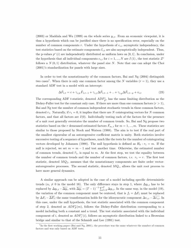
In order to test the nonstationarity of the common factors, Bai and Ng (2004) distinguish

two cases7 . When there is only one common factor among the N variables (r = 1), they use a

standard ADF test in a model with an intercept:

�F1;t = c+ i;0 F1;t�1 + i;1�F1;t�1 + ::+ i;p�F1;t�p + vi;t (23)

The corresponding ADF t-statistic, denoted ADF cbF , has the same limiting distribution as theDickey-Fuller test for the constant only case. If there are more than one common factors (r > 1),

Bai and Ng test the number of common independent stochastic trends in these common factors,

denoted r1. Naturally, if r1 = 0, it implies that there are N cointegrating vectors for N common

factors, and that all factors are I(0). Individually testing each of the factors for the presence

of a unit root generally overstates the number of common trends. So, Bai and Ng propose two

statistics based on the r demeaned estimated factors Fm; t for m = 1; :::;m. These statistics are

similar to those proposed by Stock and Watson (1988). The aim is to test if the real part of

the smallest eigenvalue of an autoregressive coe¢ cient matrix is unity. Both statistics involve

successive testing of a sequence of hypotheses, much like the tests for the number of cointegrating

vectors developed by Johansen (1988). The null hypothesis is de�ned as H0 : r1 = m. If the

null is rejected, we set m = m � 1 and test another time. Otherwise, the estimated numberof common trends, denoted br1, is equal to m. At the �rst step, we test the equality betweenthe number of common trends and the number of common factors, i.e. r1 = r. The �rst test

statistic, denoted MQf , assumes that the nonstationary components are �nite order vector-

autoregressive processes. The second statistic, denoted MQc, allows the unit root process to

have more general dynamics.

A similar approach can be adopted in the case of a model including speci�c deterministic

trends (�i 6= 0 in the model 16). The only di¤erence stays in step 1, where �yi;t has to be

replaced by �yi;t��yi; with �yi = (T � 1)�1PT

t=2�yi;t: In the same way, in the model (19),

the variation of the common component must be centered, that is ft = �Ft must be replaced

by �Ft��Ft; the same transformation holds for the idiosyncratic component �ei;t��ei;t: Inthis case, under the null hypothesis, the test statistic associated with the common component

of step 2, denoted as ADF �F (m); follows the Dickey-Fuller distribution corresponding to a

model including both a constant and a trend. The test statistic associated with the individual

component of i; denoted as ADF �e (i); follows an asymptotic distribution linked to a Brownian

bridge and similar to that of the Schmidt and Lee (1991) test.7 In the �rst working paper (Bai and Ng, 2001), the procedure was the same whatever the number of common

factors and was only based on ADF tests.

11

As argued by Banerjee and Zanghieri (2003), the implementation of the Bai and Ng (2004)

test, as it has been described here, clearly illustrates the importance of co-movements across

individuals. Indeed, for panels characterized by a strong cross-sectional dependency, the Bai and

Ng tests � by taking account the common factors across series � accept the null hypothesis of

a unit root in the factors, leading to the conclusion that the series is nonstationary. To conclude,

note that the simulations made by Bai and Ng (2004) show that their test gives satisfactory

results in terms of size and power, even for moderate panel sample sizes (N = 20).

3.2 The Phillips and Sul (2003a) and Moon and Perron (2004a) tests

In contrast to Bai and Ng (2001), Phillips and Sul (2003a) and Moon and Perron (2004a) directly

test the presence of a unit root in the observable series yi;t: Indeed, they do not proceed to

separate tests on the individual and common components. Beyond this fundamental di¤erence,

there exists some similarities between the two approaches due to the use of a factor model.

We present here in detail the Moon and Perron (2004a) test which allows for the most general

speci�cation of the common components.

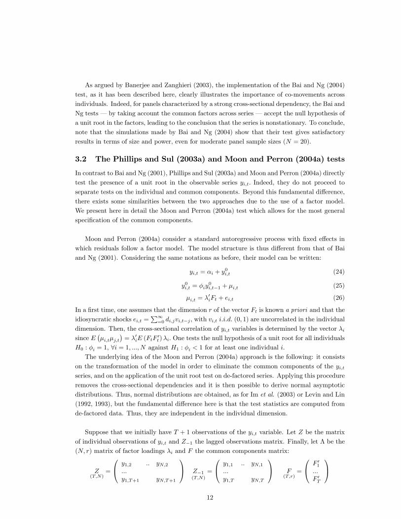
Moon and Perron (2004a) consider a standard autoregressive process with �xed e¤ects in

which residuals follow a factor model. The model structure is thus di¤erent from that of Bai

and Ng (2001). Considering the same notations as before, their model can be written:

yi;t = �i + y0i;t (24)

y0i;t = �iy0i;t�1 + �i;t (25)

�i;t = �0iFt + ei;t (26)

In a �rst time, one assumes that the dimension r of the vector Ft is known a priori and that the

idiosyncratic shocks ei;t =P1

=0 di;jvi;t�j ; with vi;t i:i:d: (0; 1) are uncorrelated in the individual

dimension. Then, the cross-sectional correlation of yi;t variables is determined by the vector �isince E

��i;t�j;t

�= �0iE (FtF

0t )�i: One tests the null hypothesis of a unit root for all individuals

H0 : �i = 1; 8i = 1; :::; N against H1 : �i < 1 for at least one individual i:

The underlying idea of the Moon and Perron (2004a) approach is the following: it consists

on the transformation of the model in order to eliminate the common components of the yi;tseries, and on the application of the unit root test on de-factored series. Applying this procedure

removes the cross-sectional dependencies and it is then possible to derive normal asymptotic

distributions. Thus, normal distributions are obtained, as for Im et al. (2003) or Levin and Lin

(1992, 1993), but the fundamental di¤erence here is that the test statistics are computed from

de-factored data. Thus, they are independent in the individual dimension.

Suppose that we initially have T + 1 observations of the yi;t variable. Let Z be the matrix

of individual observations of yi;t and Z�1 the lagged observations matrix. Finally, let � be the

(N; r) matrix of factor loadings �i and F the common components matrix:

Z(T;N)

=

0@ y1;2 :: yN;2:::y1;T+1 yN;T+1

1A Z�1(T;N)

=

0@ y1;1 :: yN;1:::y1;T yN;T

1A F(T;r)

=

0@ F 01:::F 0T

1A12

As previously mentioned, the idea of Moon and Perron (2004a) consists in testing the unit

root on the de-factored series. Suppose that the parameters of � are known. The de-factored

data are written as the projection of Z to the space orthogonal to the factor loadings (i.e. the

space generated by the columns of �): Indeed, to simplify, consider the model (25) under the

null hypothesis of a unit root (�i = 1) and in the absence of �xed e¤ects (�i = 0), written in a

vectorial form:

Z = Z�1 + F �0 + e

where e is the (T;N) idiosyncratic components matrix. Let Q� = IN� � (�0�)�1�0 be the

projection matrix to the space orthogonal to the factor loadings: By right-multiplying by Q�;

the model can be expressed from de-factored data ZQ�:

ZQ� = Z�1Q� + eQ� (27)

The projection ZQ� corresponds to de-factored data, while the residuals eQ� do not exhibit, by

construction, any cross-sectional correlation. From these de-factored data, the unit root test will

be implemented. Moon and Perron construct a test statistic from the pooled estimator8 (�i =

�j) of the autoregressive root. More speci�cally, they consider a corrected pooled estimator,

due to the possible cross-units autocorrelation of the residuals eQ�:

b�+pool = trace (Z�1Q�Z 0)�NT�etrace

�Z�1Q�Z 0�1

� (28)

where �e = N�1PN

i=1 �ie; �

ie is the sum of positive autocovariances of the idiosyncratic com-

ponents:

�ie =

1Xl=1

1Xj=0

di;jdi;j+l

From this estimator b�+pool, Moon and Perron propose two test statistics of the null hypothesisof a unit root, denoted as ta and tb respectively. These two statistics converge, assuming T and

N tend to in�nity and N=T tends to 0.

ta =TpN�b�+pool � 1�p2 4e=w

4e

d�!T;N!1

N (0; 1) (29)

tb = TpN�b�+pool � 1�

s1

NT 2trace

�Z�1QZ 0�1

� w2e 4e

d�!T;N!1

N (0; 1) (30)

The quantities w2e and 4e respectively correspond to the means on N of the individual

long-term variances w2e;i and of squared individual long-term variances 4e;i of the idiosyncratic

component ei;t with w2e;i =�P1

j=0 di;j

�2: If the calculated statistic ta (or tb) is lower than the

normal critical level, the null hypothesis of a unit root is rejected for all individuals.

Note that we have the same TpN convergence rate of the pooled estimator (corrected or

no) of the autoregressive root as the one obtained in the Levin and Lin model. This is not

surprising since, after having removed the cross unit dependencies in the Phillips and Moon

8This choice is justi�ed by the fact that this estimate simpli�es the study of asymptotic distributions, andallows for the analysis of the test under the near unit root local alternative.

13

model, one obtains on transformed data a model with common autoregressive root (pooled

estimator) similar to that of Levin and Lin under the cross-unit independency hypothesis.

Since the idiosyncratic component ei;t is not observed, the quantities w2e , �e and 4e are

unknown. The de�nitions (29) and (30) are not directly feasible. In order to implement these

tests, two (linked) complements must be added:

1. An estimate of common and idiosyncratic components: more speci�cally, an estimate bQ�of the projection matrix to the space orthogonal to the factor loadings.

2. Estimates of the long-term variances ( bw2e and b 4e) and of the positive autocovariances sum(b�e); construct from the individual components estimations bei;t:

Estimation of the projection matrixAs Bai and Ng, Moon and Perron suggest to estimate � by a principal component analysis

on the residuals. One begins with the estimation of the residuals �i;t from the model (25). To

do this, one uses a pooled estimator b�pool on original individual centered data to account for�xed e¤ects: b� = eZ � b�pool eZ�1 (31)

where eZ = QxZ and Qx = IT � T�1lT l0T where lT = (1; :::; 1)0; the pooled estimator being

de�ned as b�pool =trace� eZ 0�1 eZ� =trace� eZ 0�1 eZ�1� : From the residuals b�; a principal componentanalysis is applied. An estimate e� of the (N; r) matrix of common components coe¢ cients

ispN times a matrix whose columns are de�ned by the r eigenvectors associated with the r

largest eigenvalues of the matrix b�0b�: Moon and Perron propose a re-scaled estimate b�:b� = e�� 1

Ne�0e�� 1

2

(32)

From this estimate b�; one de�nes an estimate of the projection matrix bQ� which will allow usto obtain an estimation of the idiosyncratic components:

bQ� = IN � b��b�0b���1 b�0 (33)

An estimation of the de-factored data is thus de�ned by eZ bQ�:One can deduce a pooled correctedestimate b�+pool of the autoregressive root only on these de-factored components according to (28),replacing ZQ� by eZ bQ�.Estimation of the long-term variancesAn estimate of the idiosyncratic component is then de�ned as be = b� bQ�: Let bei;t be the

individual component of the unit i residuals at time t: For each individual i = 1; :::; N; one

de�nes the residual empirical autocovariance:

b�i (j) = 1

T

T�jXt=1

bei;tbei;t+j14

From b�i (j) ; one constructs a kernel-type estimator of the long-term variance and of the positiveautocovariances sum as:

bw2e;i = T�1Xj=�T+1

w (qi; j) b�i (j) (34)

b�e;i = T�1Xj=1

w (qi; j) b�i (j) (35)

where w (qi; j) is a kernel function and qi a truncation parameter. Finally, one has to de�ne

the estimates of the means of the individual long-term variances:

bw2e = 1

N

NXi=1

bw2e;i b�e = 1

N

NXi=1

b�e;i b 4e = 1

N

NXi=1

� bw2e;i�2 (36)

Let eta and etb be the statistics de�ned by equations (29) and (30) substituting w2e , �e and 4e by their estimates. eta and etb converge to normal laws if the kernel functions and truncationparameter q satisfy three hypotheses. Moon and Perron use a QS kernel-type function:

w (qi; j) =25

12�2 x2

�sin (6�x=5)

6�x=5� cos

�6�x

5

��for x =

j

qi

where the optimal truncation parameter qi is de�ned as:

qi = 1:3221

264 4b�2i;1Ti�1� b�2i;1�4

3751=5

where b�2i;1 is the �rst-order autocorrelation estimate of the individual component bei;t of unit i:Phillips and Sul (2003a) consider a rather more restrictive model than Moon and Perron

(2004a) since it contains only one factor independently distributed across time. The common

factors vector Ft reduces to a variable �t N:i:d: (0; 1) : Beyond this point, the main di¤erence

stays in the approach used to remove the common factors: Phillips and Sul adopt a moment

method instead of a principal component analysis. The underlying idea is to test the unit

root on orthogonalized data: since these data are independent in the individual dimension,

it is possible to apply the �rst generation unit root tests. Thus, from the estimates of the

individual autoregressive roots on orthogonalized data, Phillips and Sul construct various unit

root statistics: mean statistics similar to those of Im et al. (2003), or statistics based on p-values

combinations associated with individual unit root tests.

3.3 The Choi tests

Like Moon and Perron (2004a), Choi (2002) tests the unit root hypothesis using the modi�ed

observed series yi;t that allows the elimination of the cross-sectional correlations and the poten-

tial deterministic trend components. However, if the principle of the Choi (2002) approach is

globally similar to that of Moon and Perron, it di¤ers in two main points. First, Choi considers

an error-component model:

yi;t = �i + �t + vi;t (37)

15

vi;t =

piXj=1

di;jvi;t�j + "i;t (38)

where "i;t is i:i:d:�0; �2";i

�and independently distributed across individuals. The time e¤ect �t

is represented by a weakly stationary process. In this model, in contrast to Bai and Ng (2001)

and Moon and Perron (2004a), there exists only one common factor (r = 1) represented by the

time e¤ect �t. More fundamentally, the Choi model assumes that the individual variables yi;tare equally a¤ected by the time e¤ect (i.e. the unique common factor). Here, we have a great

di¤erence with Phillips and Sul (2003a): they also consider only one common factor, but they

assume a heterogeneous speci�cation of the sensitivity to this factor, like �i�t: Choi justi�es his

choice by the fact that the logarithmic transformation of the model (37) allows us to introduce

such a sensitivity. Moreover in the Choi model, it is possible to test the weak stationarity

hypothesis of the �t process, while it is not feasible with a heterogenous sensitivity. This is

an important point since, from a macroeconomic viewpoint, these time e¤ects are supposed to

capture the breaks in the international conjuncture, and nothing guarantees that these e¤ects

are stationary.

In the model (37), one tests the null hypothesis of a unit root in the idiosyncratic component

vi;t for all individuals, that can be written H0 :Ppi

j=1 di;j = 1; 8i = 1; :::; N; against the

alternative hypothesis that there exists some individuals i such thatPpi

j=1 di;j < 1:

The second di¤erence with the Moon and Perron (2004a) approach, linked to a certain extent

to the model speci�cation, stays in the orthogonalization of the individual series yi;t that will

be used for a unit root test only on the individual component. To eliminate the cross-sectional

correlations, Choi insulates vi;t by eliminating the intercept (individual e¤ect) �i; but also, and

more importantly, the common error term �t (time e¤ect). To suppress these deterministic

components, Choi use a two-step procedure: the use of the Elliott, Rothenberg et Stock (1996)

approach, hereafter ERS, to remove the intercept, and the suppression of the time e¤ect by

cross-sectional demeaning. Indeed, when the vi;t component is stationary, OLS provides a fully

e¢ cient estimator of the constant term. However, when vi;t is I (1) or presents a near unit root,

the ERS approach � that estimates the constant term on quasi-di¤erenced data using GLS �

in �ne allows to obtain better �nite sample properties for the unit root tests. For this reason,

the Choi (2002) test constitutes, to our knowledge, the �rst extension of the ERS approach in

a panel context. Let us now describe the two steps of the individual series orthogonalization.

Step 1: If one assumes that the largest root of the vi;t process is 1 + c=T (near unit root

process), for all i = 1; :::; N; one constructs two quasi-di¤erenced series eyi;t and eci;t suchthat, for t � 2 :

eyi;t = yi;t � �1 + c

T

�yi;t�1 eci;t = 1� �1 + c

T

�(39)

Choi considers the value given by ERS in the case of a model without time trend, that is

c = �7: Using GLS, one regresses eyi;t on the deterministic variable eci;t: Let b�i be the GLSestimate obtained for each individual i on quasi-di¤erenced data. For T large enough,

one has:

yi;t � b�i ' �t � �1 + vi;t � vi;116

whatever the process vi;t being I (1) or near-integrated. Then, one has to eliminate the

common component �t that can induce correlation across individuals. This is the aim of

the second step.

Step 2: Choi suggests to demean yi;t � b�i cross-sectionally and to de�ne a new variable zi;tsuch that:

zi;t = (yi;t � b�i)� 1

N

NXi=1

(yi;t � b�i) (40)

Indeed, given the previous results, for each individual i = 1; :::; N; one can show that:

zi;t ' (vi;t � vt)� (vi;1 � v1)

where vt = (1=N)PN

i=1 vi;t. Thus, the deterministic components �i and �t are removed

from the de�nition of zi;t: The processes zi;t can be considered as independent in the

individual dimension since the means v1 and vt converge in probability to 0 when N goes

to in�nity. Then, one has to run a unit root test on the transformed series zi;t:

In the case of a model with individual time trends, the approach is similar, but we have

to main di¤erences: to obtain the estimates b�i and b i (the coe¢ cient associated with theindividual trend), one regresses the series eyi;t on eci;t and edi;t = 1� c=T using GLS: Then, onechooses the value c = �13:5 given by ERS in the case of a model with a time trend. Oneconstructs zi;t such that:

zi;t = (yi;t � b�i � b it)� 1

N

NXi=1

(yi;t � b�i � b it)Given the series fzi;tgTt=2 ; one runs individual unit root tests without constant, nor trend,

whatever the considered model, since all deterministic components have been removed:

�zi;t = �izi;t�1 +

qiXj=1

�i;j�zi;t�j + ui;t (41)

For a model including a constant, Choi (2002) shows that the Dickey-Fuller t-statistic tERS�i

follows, under H0;i : �i = 0, the Dickey-Fuller limiting distribution when T and N tend to

in�nity. When there is a time trend, this statistic follows a distribution tabulated by ERS.

Again, one has to notice that these tests on time series, while being more powerful than the

standard ADF tests, are less powerful than panel tests. For this reason, Choi suggests panel

test statistics based on the individual tERS�istatistics which are independent. Using its previous

work (Choi, 2001), Choi (2002) proposes three statistics based on combinations of signi�cance

levels of individual tests:

Pm = �1pN

NXi=1

[ln (pi) + 1] (42)

Z = � 1pN

NXi=1

��1 (pi) (43)

17

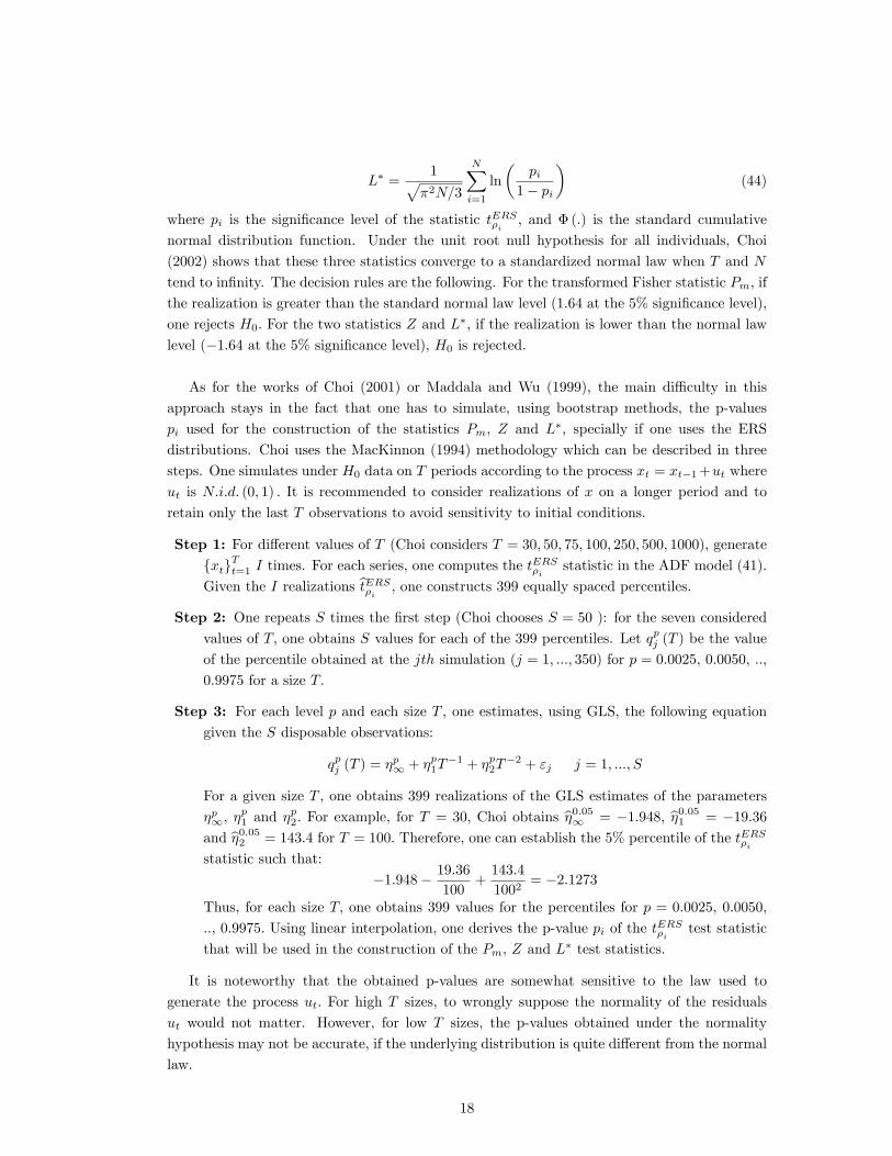
L� =1p�2N=3

NXi=1

ln

�pi

1� pi

�(44)

where pi is the signi�cance level of the statistic tERS�i; and � (:) is the standard cumulative

normal distribution function. Under the unit root null hypothesis for all individuals, Choi

(2002) shows that these three statistics converge to a standardized normal law when T and N

tend to in�nity. The decision rules are the following. For the transformed Fisher statistic Pm; if

the realization is greater than the standard normal law level (1.64 at the 5% signi�cance level),

one rejects H0: For the two statistics Z and L�; if the realization is lower than the normal law

level (�1:64 at the 5% signi�cance level), H0 is rejected:

As for the works of Choi (2001) or Maddala and Wu (1999), the main di¢ culty in this

approach stays in the fact that one has to simulate, using bootstrap methods, the p-values

pi used for the construction of the statistics Pm; Z and L�, specially if one uses the ERS

distributions. Choi uses the MacKinnon (1994) methodology which can be described in three

steps. One simulates under H0 data on T periods according to the process xt = xt�1+ut where

ut is N:i:d: (0; 1) : It is recommended to consider realizations of x on a longer period and to

retain only the last T observations to avoid sensitivity to initial conditions.

Step 1: For di¤erent values of T (Choi considers T = 30; 50; 75; 100; 250; 500; 1000); generatefxtg

Tt=1 I times. For each series, one computes the t

ERS�i

statistic in the ADF model (41).

Given the I realizations btERS�i; one constructs 399 equally spaced percentiles.

Step 2: One repeats S times the �rst step (Choi chooses S = 50 ): for the seven consideredvalues of T; one obtains S values for each of the 399 percentiles. Let qpj (T ) be the value

of the percentile obtained at the jth simulation (j = 1; :::; 350) for p = 0.0025, 0.0050, ..,

0.9975 for a size T:

Step 3: For each level p and each size T , one estimates, using GLS, the following equationgiven the S disposable observations:

qpj (T ) = �p1 + �p1T

�1 + �p2T�2 + "j j = 1; :::; S

For a given size T , one obtains 399 realizations of the GLS estimates of the parameters

�p1; �p1 and �

p2: For example, for T = 30; Choi obtains b�0:051 = �1:948; b�0:051 = �19:36

and b�0:052 = 143:4 for T = 100: Therefore, one can establish the 5% percentile of the tERS�i

statistic such that:

�1:948� 19:36100

+143:4

1002= �2:1273

Thus, for each size T; one obtains 399 values for the percentiles for p = 0:0025, 0.0050,

.., 0.9975: Using linear interpolation, one derives the p-value pi of the tERS�itest statistic

that will be used in the construction of the Pm; Z and L� test statistics:

It is noteworthy that the obtained p-values are somewhat sensitive to the law used to

generate the process ut: For high T sizes, to wrongly suppose the normality of the residuals

ut would not matter. However, for low T sizes, the p-values obtained under the normality

hypothesis may not be accurate, if the underlying distribution is quite di¤erent from the normal

law.

18

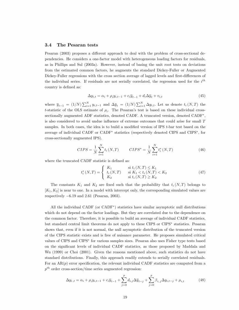
3.4 The Pesaran tests

Pesaran (2003) proposes a di¤erent approach to deal with the problem of cross-sectional de-

pendencies. He considers a one-factor model with heterogeneous loading factors for residuals,

as in Phillips and Sul (2003a). However, instead of basing the unit root tests on deviations

from the estimated common factors, he augments the standard Dickey-Fuller or Augmented

Dickey-Fuller regressions with the cross section average of lagged levels and �rst-di¤erences of

the individual series. If residuals are not serially correlated, the regression used for the ith

country is de�ned as:

�yi;t = �i + �iyi;t�1 + ciyt�1 + di�yt + vi;t (45)

where yt�1 = (1=N)PN

i=1 yi;t�1 and �yt = (1=N)PN

i=1�yi;t: Let us denote ti (N;T ) the

t-statistic of the OLS estimate of �i. The Pesaran�s test is based on these individual cross-

sectionally augmented ADF statistics, denoted CADF. A truncated version, denoted CADF�,

is also considered to avoid undue in�uence of extreme outcomes that could arise for small T

samples. In both cases, the idea is to build a modi�ed version of IPS t-bar test based on the

average of individual CADF or CADF� statistics (respectively denoted CIPS and CIPS�, for

cross-sectionally augmented IPS).

CIPS =1

N

NXi=1

ti (N;T ) CIPS� =1

N

NXi=1

t�i (N;T ) (46)

where the truncated CADF statistic is de�ned as:

t�i (N;T ) =

8<: K1

ti (N;T )K2

si ti (N;T ) � K1

si K1 < ti (N;T ) < K2

si ti (N;T ) � K2

(47)

The constants K1 and K2 are �xed such that the probability that ti (N;T ) belongs to

[K1;K2] is near to one. In a model with intercept only, the corresponding simulated values are

respectively �6:19 and 2:61 (Pesaran, 2003).

All the individual CADF (or CADF�) statistics have similar asymptotic null distributions

which do not depend on the factor loadings. But they are correlated due to the dependence on

the common factor. Therefore, it is possible to build an average of individual CADF statistics,

but standard central limit theorems do not apply to these CIPS or CIPS� statistics. Pesaran

shows that, even if it is not normal, the null asymptotic distribution of the truncated version

of the CIPS statistic exists and is free of nuisance parameter. He proposes simulated critical

values of CIPS and CIPS� for various samples sizes. Pesaran also uses Fisher type tests based

on the signi�cant levels of individual CADF statistics, as those proposed by Maddala and

Wu (1999) or Choi (2001). Given the reasons mentioned above, such statistics do not have

standard distributions. Finally, this approach readily extends to serially correlated residuals.

For an AR(p) error speci�cation, the relevant individual CADF statistics are computed from a

pth order cross-section/time series augmented regression:

�yi ;t = �i + �iyi;t�1 + ciyt�1 +

pXj=0

di;j�yt�j +

pXj=0

�i; j�yi;t�j + �i;t (48)

19

4 A second generation of tests: other approaches

There is a second approach to model the cross-sectional dependencies, which is more general

than those based on dynamic factors models or error component models. It consists in im-

posing few or none restrictions on the covariance matrix of residuals. It is in particular the

solution adopted in O�Connell (1998), Maddala and Wu (1999), Taylor and Sarno (1998), Chang

(2002, 2004). Such an approach raises some important technical problems. With cross-sectional

dependencies, the usual Wald type unit root tests based on standard estimators have limit dis-

tributions that are dependent in a very complicated way upon various nuisance parameters

de�ning correlations across individual units. There does not exist any simple way to eliminate

these nuisance parameters.

The �rst attempt to deal with this problem was done in O�Connell (1998). He considers

a covariance matrix similar as that would arise in an error component model with mutually

independent random time e¤ects and random individual e¤ects. However, this speci�cation

of cross-sectional correlations remains too speci�c to be widely used. Another attempt was

proposed in Maddala andWu (1999). They propose to way out the problem by using a bootstrap

method to get the empirical distributions of the LL, IPS or Fisher�s type test statistics in order to

make inferences. Their approach is technically di¢ cult to implement since it requires bootstrap

methods for panel data. Besides, as pointed out by Maddala and Wu, the bootstrap methods

result in a decrease of the size distortions due to the cross-sectional correlations, although it

does not eliminate them. So, the bootstrap versions of the �rst generation tests performs much

better, but do not provide the validity of using bootstrap methodology. More recently, a second

generation bootstrap unit root test has been proposed by Chang (2004). He considers a general

framework in which each panel is driven by a heterogeneous linear process, approximated by

a �nite order autoregressive process. In order to take into account the dependency among the

innovations, Chang proposes a unit root test based on the estimation on the entire system of

N equations. The critical values are then computed by a Bootstrap method.

Another solution consists in using the instrumental variable (IV thereafter) to solve the

nuisance parameter problem due to cross-sectional dependency. It is the solution adopted in

Chang (2002). The Chang (2002) testing procedure is as follows. In a �rst step, for each cross-

section unit, he estimates the autoregressive coe¢ cient from a usual ADF regression using the

instruments generated by an integrable transformation of the lagged values of the endogenous

variable. He then constructs N individual t-statistics for testing the unit root based on these N

nonlinear IV estimators. For each unit, this t-statistic has limiting standard normal distribution

under the null hypothesis. In a second step, a cross-sectional average of these individual unit

test statistics is considered, as in IPS.

Let us consider the following ADF model:

�yi;t = �i + �iyi;t�1 +

piXj=1

�i;j�yi;t�j + "i;t (49)

where "i;t are i:i:d:�0; �2"i

�across time periods, but are allowed to be cross-sectionally de-

20

pendent. To deal with this dependency, Chang uses the instrument generated by a nonlinear

function F (yi;t�1) of the lagged values yi;t�1: This function F (:) is called the Instrument Gen-

erating Function (IGF thereafter). It must be a regularly integrable function which satis�esR1�1 xF (x) dx 6= 0. This assumption can be interpreted as the fact that the nonlinear instru-ment F (:) must be correlated with the regressor yi;t�1:

Let xi;t be the vector of lagged demeaned di¤erences (�yi;t�1; :::;�yi;t�pi)0 and Xi =

(xi;pi+1; :::; xi;T )0 the corresponding (T; pi) matrix. De�ne yl;i = (yi;pi ; :::; yi;T�1)

0 the vec-

tor of lagged values and "i = ("i;pi+1; :::; "i;T )0 the vector of residuals. Under the null, the

nonlinear IV estimator of the parameter �i; denoted b�i; is de�ned as:b�i =

hF (yl;i)

0yl;i � F (yl;i)0Xi (X 0

iXi)�1X 0iyl;i

i�1hF (yl;i)

0"i � F (yl;i)0Xi (X 0

iXi)�1X 0i"i

i(50)

The variance of this IV estimator is:

b�2b�i = b�2"i hF (yl;i)0 yl;i � F (yl;i)0Xi (X 0iXi)

�1X 0iyl;i

i�2hF (yl;i)

0F (yl;i)� F (yl;i)0Xi (X 0

iXi)�1X 0iF (yl;i)

i(51)

where b�2"i = (1=T )PT

t=1 b"2i;t denotes the usual variance estimator. Chang shows that the t-ratio used to test the unit root hypothesis, denoted Zi; asymptotically converges to a standard

normal distribution if a regularly integrable function is used as an IGF.

Zi =b�ib�b�i d�!

T!1N (0; 1) for i = 1; :::; N (52)

This asymptotic Gaussian result is very unusual and entirely due to the nonlinearity of the

IV. Chang provides several examples of regularly integrable IGFs. Moreover, the asymptotic

distributions of individual Zi statistics are independent across cross-sectional units. So, panel

unit root tests based on the cross-sectional average of these individual independent statistics

can be implemented. Chang proposes an average IV t-ratio statistic, denoted SN and de�ned

as:

SN =1pN

NXi=1

Zi (53)

The factor N�1=2 is used just as a normalization factor. In an asymptotically balanced panel in

a weak sense and more over in balanced panel as in our case, this statistic has a limit standard

normal distribution. This result appears similar to those obtained under the cross-sectional

independence assumption, but the limit theories are very di¤erent in both cases. Finally, the

model with individual e¤ects can be analyzed similarly using demeaned data.

This approach is very general and has good �nite sample properties (see Chang, 2002).

According to the Chang�s simulations, the IV nonlinear test performs better than the IPS tests

in terms of both �nite sample sizes and powers. However, a recent paper of Im and Pesaran

(2003) shows that the asymptotic independence of the IV non linear t-statistics is valid only

21

under the condition that N ln (T ) =pT ! 0 when N and T tend to in�nity. The authors

remark that this condition is unlikely to hold in practice except when N is small. Besides,

their simulations based on common factor model, show that this test su¤ers from very large

size distortions even in the case previously mentioned, i.e. when N is very small relative to T .

5 Conclusion

This survey gives an overview of the main unit root tests in the econometrics of panel data.

It puts forward that two directions of research have been developed since the seminal work of

Levin and Lin (1992), leading to two generations of panel unit root tests. The �rst one concerns

heterogeneous modellings with the contributions of Im, Pesaran and Shin (1997), Maddala and

Wu (1999), Choi (2001) and Hadri (2000). The second area of research, more recent, aims to

take into account the cross-sectional dependencies. This last category of tests is still under

development, given the diversity of the potential cross-sectional correlations.

References

Bai, J. and Ng, S. (2001), �A PANIC Attack on Unit Roots and Cointegration�, Mimeo,

Boston College, Department of Economics.

Bai, J. and Ng, S. (2002), �Determining the Number of Factors in Approximate Factor

Models�, Econometrica, 70(1), 191-221.

Bai, J. and Ng, S. (2004), �A PANIC Attack on Unit Roots and Cointegration�, Economet-

rica, 72(4), 1127-1178.

Baltagi, B.H. and Kao, C. (2000), �Nonstationary Panels, Cointegration in Panels and

Dynamic Panels: a Survey�, Advances in Econometrics, 15, Elsevier Science, 7-51.

Banerjee, A. (1999), �Panel Data Unit Root and Cointegration: an Overview�, Oxford Bul-

letin of Economics and Statistics, Special Issue, 607-629.

Banerjee, A., Marcellino, M. and Osbat, C. (2000), �Some Cautions on the Use of Panel

Methods for Integrated Series of Macro-economic Data�, Working Paper 170, IGIER.

Banerjee, A. and Zanghieri, P. (2003), �A New Look at the Feldstein-Horioka Puzzle

Using an Integrated Panel�, Working Paper CEPII 2003-22.

Chang, Y. (2002), �Nonlinear IV Unit Root Tests in Panels with Cross�Sectional Depen-

dency�, Journal of Econometrics, 110, 261-292.

Chang, Y. (2004), �Bootstrap Unit Root Tests in Panels with Cross-Sectional Dependency�,

Journal of Econometrics, 120, 263-293.

Choi, I. (2001), �Unit Root Tests for Panel Data�, Journal of International Money and Fi-

nance, 20, 249-272.

Choi, I. (2002), �Combination Unit Root Tests for Cross-Sectionally Correlated Panels�,

Mimeo, Hong Kong University of Science and Technology.

22

Elliott, G., Rothenberg, T. and Stock, J. (1996), �E¢ cient Tests for an AutoRegressive

Unit Root�, Econometrica, 64, 813-836.

Fisher, R.A. (1932), Statistical Methods for Research Workers, Oliver and Boyd, Edinburgh.

Hadri, K. (2000), �Testing for Unit Roots in Heterogeneous Panel Data�, Econometrics Jour-

nal, 3, 148-161.

Harris, R.D.F. and Tzavalis, E. (1999), �Inference for Unit Roots in Dynamic Panels where

the Time Dimension is Fixed�, Journal of Econometrics, 91, 201-226.

Hsiao, C. (1986), �Analysis of Panel Data�, Econometric society Monographs N0 11. Cam-

bridge University Press.

Im, K.S. and Pesaran, M.H. (2003), �On the Panel Unit Root Tests Using Nonlinear In-

strumental Variables�, Mimeo, University of Southern California.

Im, K.S., Pesaran, M.H., and Shin, Y. (1997), �Testing for Unit Roots in Heterogenous

Panels�, DAE, Working Paper 9526, University of Cambridge.

Im, K.S., Pesaran, M.H., and Shin, Y. (2003), �Testing for Unit Roots in Heterogeneous

Panels�, Journal of Econometrics, 115, 1, 53-74.

Johansen, S. (1988), �Statistical Analysis of Cointegration Vectors�, Journal of Economic

Dynamics and Control, 12, 231-254.

Kwiatkowski, D., Phillips, P.C.B., Schmidt, P. and Shin, Y. (1992), �Testing the Null

Hypothesis of Stationarity against the Alternative of a Unit Root�, Journal of Econometrics,

54, 91-115.

Levin, A. and Lin, C.F. (1992), �Unit Root Test in Panel Data: Asymptotic and Finite

Sample Properties�, University of California at San Diego, Discussion Paper 92-93.

Levin, A. and Lin, C.F. (1993), �Unit Root Test in Panel Data: New Results�, University

of California at San Diego, Discussion Paper 93-56.

Levin, A., Lin, C.F., and Chu., C.S.J. (2002), �Unit Root Test in Panel Data: Asymptotic

and Finite Sample Properties�, Journal of Econometrics, 108, 1-24.

MacKinnon, J.G. (1994), �Approximate Asymptotic Distribution Functions for Unit Root

and Cointegration�, Journal of Business and Economic Statistics, 12, 167-176.

Maddala, G.S. and Wu, S. (1999), �A Comparative Study of Unit Root Tests with Panel

Data and a New Simple Test�, Oxford Bulletin of Economics and Statistics, special issue, 631-

652.

Moon, H. R. and Perron, B. (2004a), �Testing for a Unit Root in Panels with Dynamic

Factors�, Journal of Econometrics, 122, 81-126

Moon, H. R. and Perron, B. (2004b), �Asymptotic Local Power of Pooled t-Ratio Tests

for Unit Roots in Panels with Fixed E¤ects�, Mimeo, University of Montréal.

Moon, H. R., Perron, B. and Phillips, P.C.B (2003), �Incidental Trends and the Power

of Panel Unit Root Tests�, Mimeo, University of Montréal.

23

Nabeya, S., (1999), �Asymptotic Moments of some Unit Root Test Statistics in the Null Case�,

Econometric Theory, 15, 139-149.

OConnell, P. (1998), �The Overvaluation of Purchasing Power Parity�, Journal of Interna-

tional Economics, 44, 1-19.

Pesaran,H.M. (2003), �A Simple Panel Unit Root Test in the Presence of Cross Section

Dependence�, Mimeo, University of Southern California.

Pesaran,H.M. and Smith,R (1995), �Estimating Long-Run Relationships from Dynamic

Heterogenous Panels�, Journal of Econometrics, 68, 79-113.

Phillips, P.C.B. and Moon, H. (1999), �Linear Regression Limit Theory for Nonstationary

Panel Data�, Econometrica, 67, 1057-1111.

Phillips, P.C.B. and Sul, D. (2003a), �Dynamic Panel Estimation and Homogeneity Testing

Under Cross Section Dependence�, Econometrics Journal, 6(1), 217-259.

Phillips, P.C.B. and Sul, D. (2003b), �The Elusive Empirical Shadow of Growth Conver-

gence�, Cowles Foundation Discussion Paper 1398, Yale University.

Ploberger, W. and Phillips, P.C.B. (2002), �Optimal Testing for Unit Roots in Panel

Data�, Mimeo.

Quah, D. (1994), �Exploiting Cross-Section Variations for Unit Root Inference in Dynamic

Data�, Economics Letters, 44, 9-19.

Schmidt, P. and Lee, J. (1991), �A Modi�cation of Schmidt-Phillips Unit Root Test�, Eco-

nomics Letters, 36, 285-289.

Stock, J.H and Watson, M.W. (1988), �Testing for Common Trends�, Journal of the

American Statistical Association, 83, 1097-1107.

Strauss, J. and Yigit, T. (2003), �Shortfalls of Panel Unit Root Testing�, Economics Letters,

81, 309-313.

Taylor, M.P. and Sarno, L. (1998), �The Behavior of Real Exchange Rates During the

Post-Bretton Woods Period�, Journal of International Economics, 46, 281-312.

24