Seasonal Variation versus Climate variation for Australian Tourism · 2010-10-11 · Seasonal...

Seasonal Variation versus Climate Variation for Australian Tourism

1

Seasonal Variation versus Climate variation for Australian Tourism Nada Kulendran and Larry Dwyer

Nada Kulendran

School of Economics and Finance, and Centre for Hospitality and Tourism Research,

Faculty of Business and Law, Victoria University, Melbourne, Australia

Larry Dwyer Qantas Professor of Travel and Tourism Economics

School of Marketing, Australian School of Business University of New South Wales, NSW 2052, Australia

Correspondence to Dr. Nada KulendranSenior Lecturer School of Economics and Finance City Campus Faculty of Business and Law Victoria University

P.O. Box: 14428 MCMC, Melbourne 8001 AUSTRALIA Fax: + 03 9919 4888 E-mail: [email protected]


2

DisclaimerThe technical reports present data and its analysis, meta-studies and conceptual studies, and are considered to be of value to industry, government or other researchers. Unlike the Sustainable Tourism Cooperative Research Centre’s (STCRC’s) Monograph series, these reports have not been subjected to an external peer review process. As such, the scientific accuracy and merit of the research reported here is the responsibility of the authors, who should be contacted for clarification of any content. Author contact details are e-mail: [email protected]. . The views and opinions of the authors expressed in the reports or by the authors if you contact them do not necessarily state or reflect those of the STCRC.

While all reasonable efforts have been made to gather the most current and appropriate information, the STCRC does not give any warranty as to the correctness, completeness or suitability of the information, and disclaims all responsibility for and shall in no event be liable for any errors or for any loss or damage that might be suffered as a consequence of any person acting or refraining from acting or otherwise relying on this information.

We’d love to know what you think of our new research titles. If you have five minutes to spare, please visit

our website or click on the link below to complete our online survey. STCRC Tech Report Feedback

Editor-in-ChiefProfessor David Simmons Director of Research, Sustainable Tourism Cooperative Research Centre

National Library of Australia Cataloguing-in-Publication Entry Title: Seasonal variation versus climate variation for Australian tourism / Nada Kulendran ... [et al.] ISBNs: 978-1-921785-09-2 (pbk.), 978-1-921785-59-7 (PDF) Other Authors/Contributors: CRC for Sustainable Tourism Pty Ltd, Larry Dwyer.

Copyright © CRC for Sustainable Tourism Pty Ltd 2010 All rights reserved. Apart from fair dealing for the purposes of study, research, criticism or review as permitted under the Copyright Act, no part of this book may be reproduced by any process without written permission from the publisher. Any enquiries should be directed to: General Manager, Communications and Industry Extension or Publishing Manager, [email protected] First published in Australia in 2010 by CRC for Sustainable Tourism Pty Ltd Printed in Australia (Gold Coast, Queensland)

Acknowledgements The Sustainable Tourism Cooperative Research Centre, established and supported under the Australian Government’s Cooperative Research Centres Program, funded this research.


3

CONTENTS

1. Introduction ................................................................ 5

2. A Climate Index for Tourism ................................................................ 7

3. Comparison of Seasonal Component Variation and Climate Variation by Seasons ................................... 10

4. Periodic Growth in Seasonal Variation versus Periodic Growth Climate Variation by Seasons and by Origin .............................................................. 14

5. The impact of Climate Variation on Seasonal Variation .............................................................. 18

6. Conclusions .............................................................. 20

References .............................................................. 26

List of Tables Table 1: Maximum temperature, humidity and sunshine hours, September 1975-September 2009, Australia (cities, Sydney, Melbourne, Brisbane) _________________________________________________________ 8 Table 2: Extracted seasonal component mean values by seasons (in ‘000s visitors) ______________________ 9 Table 3: Measured Deviations between Max Temperature Variation in Australia and Seasonal Component Variation by Season and by Origin Country ____________________________________________________ 11 . Table 4: Measured Deviation between Humidity Variation in Australia and Seasonal Component Variation by Season and by Origin Country ______________________________________________________________ 12 Table 5: Measured Deviation between Hours of Sunshine in Australia and Seasonal Component Variation by Season and by Origin Country ______________________________________________________________ 13 Table 6: Quarters showing the Minimum Deviation between Climate Variation and Seasonal Variation, for Each Origin _________________________________________________________________________________ 14 Table 7: Measured Distances between Change in Temperature in Australia and Change in Seasonal Variation by Quarters and by Origin Country __________________________________________________________ 14 Table 8: Measured Distances between Change in Humidity and Change in Seasonal by Quarters and by Country ______________________________________________________________________________________ 15 Table 9: Measured Distance between Change in Hours in Sunshine and Change in Seasonal Variation by Quarters and by Country __________________________________________________________________ 16 Table 10: The Selected Quarters from the Comparison of Periodic Change in Climate Variation and Periodic Change in Seasonal Variation ______________________________________________________________ 17 Table 11: Estimated Time Series Seasonal Variation Model _______________________________________ 19 Table 12: Estimated impact of Maximum Temperature, Humidity, Sunshine Hours on Seasonal Variation ___ 19

List of Figures Figure 1: Variation in maximum temperature, humidity and sunshine hours, September 1975-September 2009, Australia (cities, Sydney, Melbourne, Brisbane) __________________________________________________ 9 Figure 2: Quarterly seasonal variation mean values by countries ____________________________________ 9 Figure 3: Distances between Temperature variation and Seasonal Variation __________________________ 11 Figure 4: Distances between Humidity Variation and Seasonal Variation ____________________________ 12 Figure 5: Distances between Hours of Sunshine Variation and Seasonal Variation _____________________ 13 Figure 6: Distances of Periodic Change in Maximum Temperature and Periodic Change in Seasonalvariation by Quarter and Country ______________________________________________________________________ 15 Figure 7: Distances of Periodic Change in Humidity Variation and Periodic Change in Seasonal Variation _ 16


4

Figure 8: Distances of Periodic Change in Hours of Sunshine Variation and Periodic Changes in Seasonal Variation _______________________________________________________________________________ 17

List of Plots Plot 1a: Holiday Arrivals to Australia from UK: 1975 September Quarter to 2009 September Quarter ______ 21 Plot 1b: Holiday Arrivals to Australia from New Zealand: 1975 September Quarter to 2009 September Quarter ______________________________________________________________________________________ 21 Plot 1c: Holiday Arrivals to Australia from USA: 1975 September Quarter to September 2009 September Quarter ________________________________________________________________________________ 22 Plot 1d: Holiday Arrivals to Australia from Japan: 1975 September Quarter to 2009 September Quarter ___ 22 Plot 2: Maximum Temperature, Relative Humidity and Sunshine Hours from 1975 September Quarter to 2009 September Quarter _______________________________________________________________________ 23 Plot 3: Extracted Seasonal Variation from Holiday Visitor Arrivals to Australia from NZ, UK, USA and Japan Using the BSM modelling Approach from 1975 September quarter to 2009 September Quarter. ___________ 23

AbstractClimate variables such as maximum temperature, humidity percentage and hours of sunshine influence holiday destination choice. So also, changes in the mean value of these climate variables in different seasons may be expected to influences the seasonal variation in holiday tourism within and between destinations. The purpose of this paper is to measure the influence of changes in these climate related variables on the seasonal variation in Australian inbound holiday tourism. The study uses data on arrivals from USA, UK, Japan and New Zealand to Australia from September 1975 to September 2009. Seasonal variation which is the respective and predictable movement around the trend line for tourism growth was first extracted from the quarterly holiday visitor arrivals time-series using the Basic Structural Model (BSM) approach. Subsequently, the influence of these climate variables on seasonal variation in different seasons was identified using the Euclidean minimum distance approach. The study findings are that maximum temperature, relative humidity and hours of sunshine variations shape the characteristic of seasonal variation of tourism flows but the effect tends to vary between seasons and countries. A time-series model was employed to measure the impact of climate variables on the seasonal variation of inbound tourism flows to Australia. The humidity percentage impacts upon seasonal variation from USA and UK whereas the hours of sunshine impacts upon seasonal variation from New Zealand. The impact of Australian temperature on seasonal variation cannot be generalised to all Australian inbound tourism markets. The impact varies between Northern Hemisphere tourism markets and Australia’s most important Southern Hemisphere market. Keywords: Seasonal variation, Climate variation, Euclidean Distance Approach, ARCH Modelling, Australian tourism


5

1. INTRODUCTION

Climate is important to international tourism because it attracts visitors who expect favourable weather conditions in their holiday destination. It is widely accepted that seasonal holiday travel is motivated by destination climate conditions, such as temperature, sunshine and humidity and environmental variables and each has been identified as important in models of destination competitiveness. (Dwyer and Kim 2003). Change in the mean value of weather pattern including temperature, humidity, and rainfall in different seasons could change the seasonal variation in holiday visitor arrivals. These elements, which influence destination choice, are of great relevance to tourism stakeholders in both the private and public sectors affecting not only the profitability of day to day operations but also the planning and design of tourism facilities to maintain destination competitiveness into the future.

Climate plays a major role in the marketing of holiday tourism to destinations. Tourism Australia jointly with government, the state/territory and travel industry promote ‘Discover Australia in Different Seasons’ by providing activities and things to do in Australia in different seasons. Tourism planners, developers and managers promote Australia by focusing on different market segments for different seasons—such as senior citizen, business travellers, conference and event planners and special interest tourists with aggressive pricing strategy. The Australia comparative advantage is that it is in Southern Hemisphere whereas Australia’s high yield major tourism markets such as USA, UK and Japan are located in the Northern Hemisphere. That is, seasons in Australia are the reverse of USA, UK and Japan. Warm and more sunshine hours in Australia compared to less sunshine hours and cold winters in USA, UK and Japan attract visitors from major markets to visit Australia to enjoy well known three ‘S’s’ in tourism: sun, sand and sea. When Australia is in winter, Europe, North America and Japan are experiencing summer, affecting visitor arrivals to Australia. New Zealand, Australia’s major inbound market is in the Southern Hemisphere. It is closer proximity to Australia and has same season and similar features including sandy beaches and culture. When Australia is in summer New Zealand is also in summer and it may attract domestic beach holiday tourism which is cheaper for New Zealanders.

The world is experiencing changes in the mean weather conditions, including temperature, humidity, rainfall

and frequency of floods, storms and droughts so on (ICCP 2007). Therefore, the change in mean weather condition in different seasons could change the seasonal variation pattern in quarterly visitor arrivals time-series,

Seasonal variation in tourism flows for any destination can be measured as the fluctuation in visitor numbers

from season to season. Hylleberg (1992) proposed the following definition of seasonality in economies generally:

‘Seasonality is the systematic, although not necessarily regular, intra-year movement caused by the changes of the weather, the calendar, and timing of decisions, directly or indirectly through the production and consumption decisions made by the agents of the economy. These decisions are influenced by endowments, the expectations and preferences of the agents’. The factors that causes the seasonal movement can be classified into three groups: 1. weather—includes temperature, precipitation, hours of sunshine 2. calendar events such as Christmas, Easter, Ramadan etc., 3. timing decisions such as school vacations, industry vacations, tax years, accounting periods, dates for

dividend and bonus payment etc.. Some of the causes such as calendar events and timing decisions may not change for a longer period but the

varying cause is the weather which is unpredictable. Weather is the mix of events that happen each day in our atmosphere including temperature, rainfall and humidity where as climate is the average weather pattern in a place over many years. Seasonal movement/seasonal variation is mainly caused by variation in mean weather condition (referred to as climate variation) in different season as the result the seasonality can be referred as climatic seasonality.

Seasonality in tourism is caused by similar conditions. Seasonal variation which is the fluctuation from


6

season to season could be constant or deterministic if the mean weather conditions in different seasons are constant. Koenig-Lewis and Bischoff (2005) reviewed past tourism seasonality studies and found that ‘natural and institutional’ factors are the two major causes for tourism seasonality. Natural factors are related to the ‘considerable variations in the climate throughout each year, in the hours of day light and of sunshine, the maximum and minimum temperatures, rainfall, snow etc.’ Institutional factors include calendar effect (timing of religious festivals such as Christmas, Easter, Ramadan etc,) and timing decisions (school vacations, industry vacations etc.). Climatic elements considered to have the greatest influence on seasonal tourism are: temperature, sunshine, radiation, precipitation, wind, humidity, and fog (Stern et al. 2000, Hamilton and Lau, 2004, Gomez 2005). Past studies (Amelung et. a.l. (2009), Stern et al. 2000, Hamilton and Lau, 2004, Gomez 2005, and Dwyer and Kim 2003) have recognized the link between climate variables and seasonal variation but no attempt has been made to quantify the impact of maximum temperature, hours of sunshine and humidity on seasonal variation using a time-series model. The importance of adopting a quantitative approach in seasonality research has recently been emphasised (Koenig-Lewis and Bischoff, 2005).

To date, tourism demand modelling studies (Crouch. 1995, Witt and Witt 1995, Lim 2006) have largely been

silent on the potential effects of climate change on destination choice. Lise and Tol (2002) state that: ‘While climate is obviously an important factor for determining seasonal tourism demand (measured by number of visitor arrivals), very few tourism demand studies have identified the link with climate. Yet, it is not known just how important climate is for the destination choice of tourists’. Studies which have recently attempted to measure the effects of climate on tourism flows include Lise and

Tol (2002) who estimated the impact of climate on total tourist arrivals and departures on world, Canada, France, Germany, Italy, Japan, Netherland, UK and USA. The authors found that climate change (represented by temperature and precipitation) will have an increasingly strong effect on tourism demand. This study used the regression analysis for the estimation procedure. In another study, Goh, Law and Mok (2008) used both the rough sets algorithms approach method and econometric analysis which consists of both quantitative economic factors and qualitative non-economic factors to measure the impact of leisure time and climate on annual Hong Kong inbound tourism demand. Focusing on long-haul USA and UK tourism demand for Hong Kong, this study showed that leisure time and climate have stronger impacts on tourist arrivals than economic factors. Hamilton, Maddision and Tol (2005) simulated international tourist flows using 1995 data on arrivals and departures for 207 countries and the impact on arrivals and departures through changes in population, per capita income, and climate change which is measured by annual average temperature. The study found that in the medium to long term, tourism will grow; however; the change from climate change is smaller than from population and income changes. Hamilton and Tol (2007) further extended their work on the Hamburg Tourism Model (HTM) to downscale by region for Germany, the UK and Ireland. They found that the impact of climate change on national tourism is different to that for regional tourism. Berrittela, Bigano, Roson, and Tol (2006) studied the economic implications of climate change induced variations in tourism demand using a world computable general equilibrium (CGE) Model. This study considered the minimal temperature variation as a climate change to estimate the impact of climate change on aggregate tourism expenditure. Taylor and Ortiz (2009) employed panel data techniques on regional tourist and climate data in the UK to estimate the influence of temperature, precipitation and sunny conditions on domestic tourism. The study found that the climate variables have significant impact on domestic tourism.

Despite the relatively large number of Australian tourism demand studies to date (Crouch, Schultz, and

Valerio 1992; Kulendran, 1996; Lim and McAleer, 2001; Divisekera, 2003 ; Kulendran and Divisekera 2005; Kulendran and Dwyer 2009), no attempt has been made to measure the impact of climate variables such as temperature, sunshine and humidity on the seasonal tourism demand for inbound tourism. Focusing as they have on variables such as origin country income, tourism price, cost of travel and special events and marketing and migration stocks and flows, these studies are vulnerable to the criticism of Lise and Tol (2002) that they ‘ have short time horizon, assuming that the climate at the tourist destination is constant. In the longer term, however, climate is not constant’.

The drawback to previous studies that have included climate variables in their tourism demand model is that,

in their emphasis on climate variation impacts on total tourism flows or tourism expenditure, they have ignored its effects on the seasonal variation in tourist flows. Thus if a destination becomes warmer due to climate change and guaranteed sunshine and heat for the holiday makers it is likely to have a positive impact on the seasonal


7

variation in holiday visitor arrivals to that destination. While the researchers have emphasised that maximum temperature, hours of sunshine and humidity are the important factors for determining the seasonal variations in the past no attempt has been made to model the seasonal variation using the climate variables.

In tourism, the inclusion of a seasonal variation in the climate variables impact study has several advantages.

First, it enables us to identify which climatic variables strongly influence the seasonal variation for different seasons. Second, it enables us to identify the differences between the climate impact and the impacts of the standard economic variables on seasonal demand. This study is the first attempt to estimate the impact of maximum temperature, hours of sunshine and humidity on the seasonal variation in tourism flows. This study quantifies the impact of temperature, hours of sunshine and humidity on seasonal variations in Australian inbound holiday tourism using a time-series model. Specifically, it considers maximum temperature, sunshine hours and relative humidity in estimating the impact of climate on the seasonal component in holiday visitor arrivals to Australia from four major source markets: New Zealand (NZ), USA, UK and Japan, using a time-series modelling approach.

The structure of the paper is as follows: Section Two provides an outline of some climate indexes for tourism

that have been constructed for different destinations. Section Three identifies the link between seasonal variation and variation in maximum temperature, sunshine hours and humidity by quarters using the Euclidean minimum distance approach. Section Four considers the time-series modelling approach to quantify the impact of maximum temperature, hours of sunshine and humidity on seasonal variation. The final section explores some policy implications of the study findings.

2. A CLIMATE INDEX FOR TOURISM

To measure the impact of climate on seasonal tourism a climate index for tourism must be developed. Previous studies have attempted to construct a tourism climate index to capture weather information relevant to specific tourist activities at a particular destination. Key variables considered in these studies are temperature, sunshine hours, humidity and wind speed. Mieczkowski, (1985) constructed a Tourism Climate Index (TCI) based on six sub-indices: Day time comfort index (CID) which is measured by maximum daily temperature (0C) and minimum daily relative humidity (%); Daily comfort index (CIA) which is measured by mean daily temperature (0C) and mean daily relative humidity (%); Perception (R) (mm); Sunshine (S) measured by daily duration of sunshine (hours); Wind speed (W) (m/s or KM/h). The index is weighted and computed as follows: TCI= 4CID + CIA+2R+2S+W indicating that more weight is given to the day time comfort index followed by precipitation and sunshine. The mapping of raw data to sub-index values depends on the kind and level of tourist activity. For example beach holidays require climatic conditions different from ski holidays. This formula was derived based on the light tourism activity such as touring. In the equation proposed by Mieczkowski, the highest weighting is given to the daytime comfort index reflecting the fact that tourist behaviour is generally more influenced by weather conditions during the daytime. Duration of sunshine hours and perception have the second highest weight because this is also related to tourist activity in the daytime. As suggested by Skinner and De Dear (2001) the classification takes no account of rainy days and assumes that rainy days are always unfavourable. In the tropics, rain can actually provide more comfortable conditions for outdoor activity because of its cooling effect and rain implies cloud, which means less intense radiation from the sun. Past studies (Matzarakis, 2001a, 2001b, Skinner and De Dear, 2001) considered solar radiation also in the TCI calculation because tourists can suffer serious ill effects from the intense sunshine. Goh, et al. (2008), constructed a climate index for Hong Kong including the following climate variables: a daytime comfort index comprising maximum daily temperature and minimum daily relative humidity; a daily comfort index which is composed of daily temperature and daily relative humidity; and ratings for precipitation in Hong Kong, duration of sunshine, and wind speed.

However, there are some draw backs in the construction of a climate index. Amelung, et. al.(2009) argue that

the TCI applies only to sightseeing and shopping and more general forms of tourism activity and it is not applicable to more climate-dependent activities such as winter sport. Different climatic variables are required for different types of climate dependent tourism activity and different locations. For example beach holiday, sightseeing and shopping holiday activity requires warm climate conditions while winter skiing holidays require cooler climatic conditions. Moreover, the assignment of weights by researchers to climatic variables is a


8

subjective process and may change according the tourist activity. Assigning weights to beach holiday tourism is different to light tourism activity such as sightseeing and shopping activity because beach tourism requires much warmer and less humidity percentage climate than the sightseeing and shopping holiday activity. Another problem is that since a TCI measures the impact of a weighted average of climatic variables on seasonal tourism demand it is not useful for discerning the effects of the individual components of the index.

To overcome the problems commonly associated with published climate change indexes as a determinant of

tourism demand this study attempts a more disaggregative approach that involves estimating the impact of individual climatic variables on tourism flows. To provide a context for the results, the study focuses on the impact of Australian climatic variables on inbound tourism demand from four of its major origin markets- UK, Japan, USA and New Zealand.

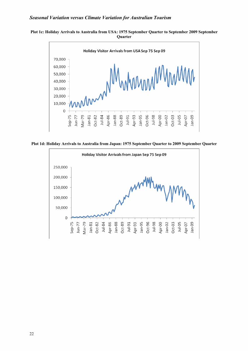
To estimate the impact of climate variation on seasonal variation this study first extracted for Australia the

seasonal variation from the quarterly holiday visitor arrivals time-series. Seasonal variation is a component of a visitor arrivals time-series which is defined as the repetitive and predictable movement around the trend line. It is detected by measuring the visitor arrivals in quarters. Plot 1 shows the seasonal variation and the trend in quarterly tourist arrivals to Australia from USA, UK, Japan and New Zealand. Quarterly visitor arrivals time-series has four components: Trend (T), Seasonal(S), Cyclical(C) and Irregular (�). To extract the seasonal (S) variation from the quarterly visitor arrivals time-series the Basic Structural Model (BSM) approach (Harvey 1989) was employed. Quarterly holiday visitor arrivals time series to Australia from USA, Japan, UK and New Zealand for the period from the September quarter 1975 to September quarter 2009 were obtained from ABS Catalog No: 3401.0. The BSM approach assumes that a time series possesses some structure, which is the sum of the unobserved components: trend, seasonal and irregular. The unobserved components model can be written as: Yt = Tt + St + �t where Yt is the quarterly visitor arrivals series, Tt is the Trend Component, St is a Seasonal Component, �t is a Irregular component which is normally distributed with (0, ��

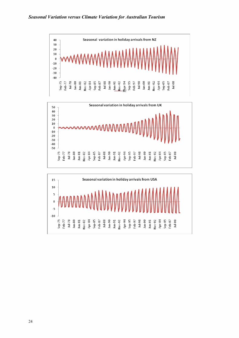
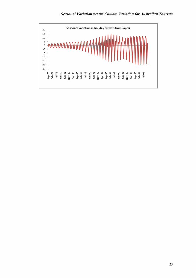
2 ). The cyclical component was not considered because main purpose of using BSM approach is to extract the seasonal variation from the quarterly time-series. The BSM of Harvey (1989) was estimated by STAMP (5.0) program. Plot 2 shows the extracted seasonal variation in holiday visitor arrival to Australia from USA, UK, Japan and New Zealand which exhibits increasing seasonal variation.

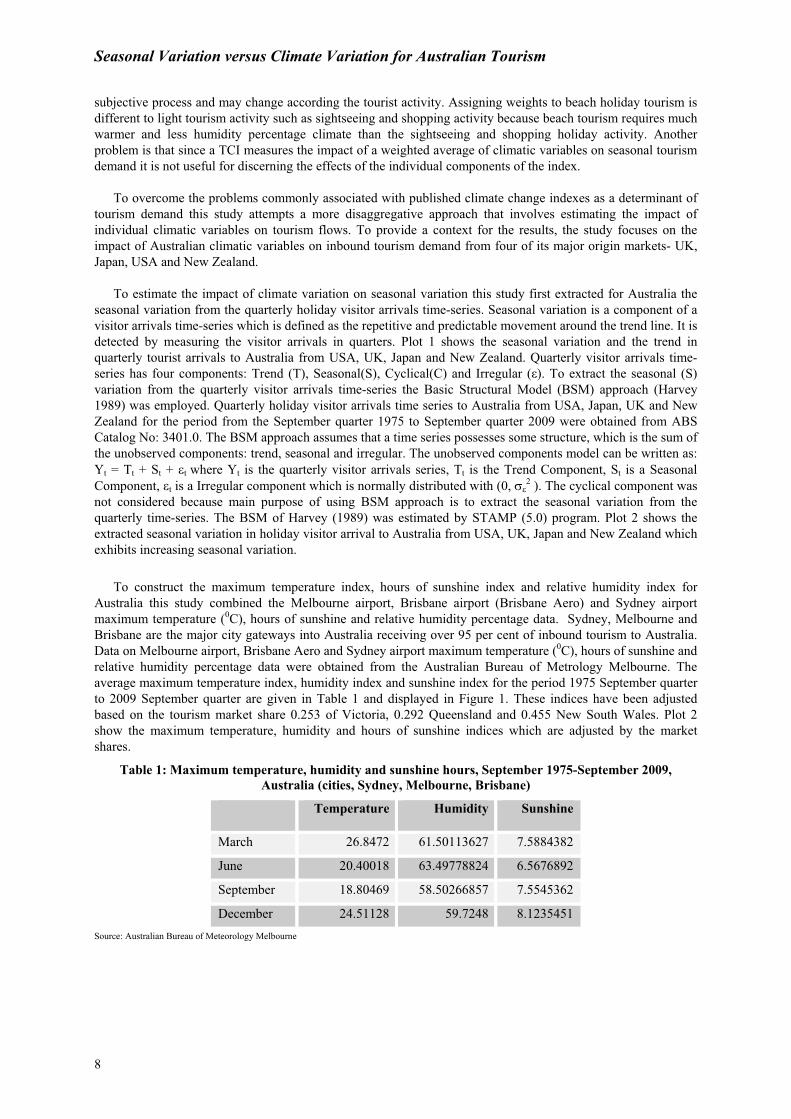
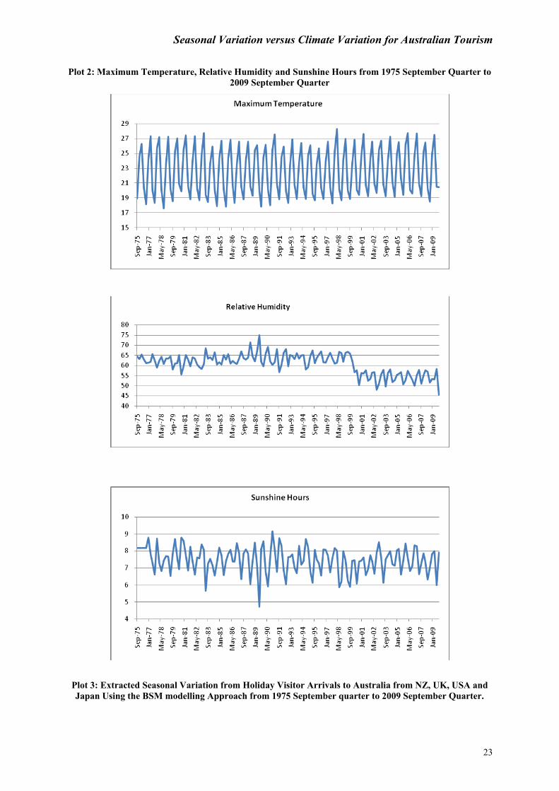
To construct the maximum temperature index, hours of sunshine index and relative humidity index for Australia this study combined the Melbourne airport, Brisbane airport (Brisbane Aero) and Sydney airport maximum temperature (0C), hours of sunshine and relative humidity percentage data. Sydney, Melbourne and Brisbane are the major city gateways into Australia receiving over 95 per cent of inbound tourism to Australia. Data on Melbourne airport, Brisbane Aero and Sydney airport maximum temperature (0C), hours of sunshine and relative humidity percentage data were obtained from the Australian Bureau of Metrology Melbourne. The average maximum temperature index, humidity index and sunshine index for the period 1975 September quarter to 2009 September quarter are given in Table 1 and displayed in Figure 1. These indices have been adjusted based on the tourism market share 0.253 of Victoria, 0.292 Queensland and 0.455 New South Wales. Plot 2 show the maximum temperature, humidity and hours of sunshine indices which are adjusted by the market shares.

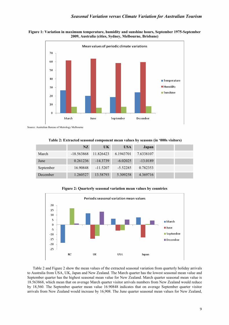
Table 1: Maximum temperature, humidity and sunshine hours, September 1975-September 2009, Australia (cities, Sydney, Melbourne, Brisbane)

Temperature Humidity Sunshine

March 26.8472 61.50113627 7.5884382

June 20.40018 63.49778824 6.5676892

September 18.80469 58.50266857 7.5545362

December 24.51128 59.7248 8.1235451 Source: Australian Bureau of Meteorology Melbourne


9

Figure 1: Variation in maximum temperature, humidity and sunshine hours, September 1975-September 2009, Australia (cities, Sydney, Melbourne, Brisbane)

Source: Australian Bureau of Metrology Melbourne

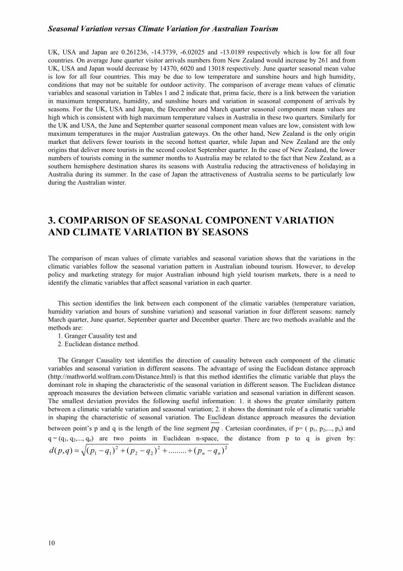
Table 2: Extracted seasonal component mean values by seasons (in ‘000s visitors)

NZ UK USA Japan

March -18.563868 11.826423 6.1943701 7.6338107

June 0.261236 -14.3739 -6.02025 -13.0189

September 16.90848 -11.5207 -5.52285 0.782353

December 1.260527 13.58793 5.309258 4.369716

Figure 2: Quarterly seasonal variation mean values by countries

Table 2 and Figure 2 show the mean values of the extracted seasonal variation from quarterly holiday arrivals to Australia from USA, UK, Japan and New Zealand. The March quarter has the lowest seasonal mean value and September quarter has the highest seasonal mean value for New Zealand. March quarter seasonal mean value is 18.563868, which mean that on average March quarter visitor arrivals numbers from New Zealand would reduce by 18,560. The September quarter mean value 16.90848 indicates that on average September quarter visitor arrivals from New Zealand would increase by 16,908. The June quarter seasonal mean values for New Zealand,


10

UK, USA and Japan are 0.261236, -14.3739, -6.02025 and -13.0189 respectively which is low for all four countries. On average June quarter visitor arrivals numbers from New Zealand would increase by 261 and from UK, USA and Japan would decrease by 14370, 6020 and 13018 respectively. June quarter seasonal mean value is low for all four countries. This may be due to low temperature and sunshine hours and high humidity, conditions that may not be suitable for outdoor activity. The comparison of average mean values of climatic variables and seasonal variation in Tables 1 and 2 indicate that, prima facie, there is a link between the variation in maximum temperature, humidity, and sunshine hours and variation in seasonal component of arrivals by seasons. For the UK, USA and Japan, the December and March quarter seasonal component mean values are high which is consistent with high maximum temperature values in Australia in these two quarters. Similarly for the UK and USA, the June and September quarter seasonal component mean values are low, consistent with low maximum temperatures in the major Australian gateways. On the other hand, New Zealand is the only origin market that delivers fewer tourists in the second hottest quarter, while Japan and New Zealand are the only origins that deliver more tourists in the second coolest September quarter. In the case of New Zealand, the lower numbers of tourists coming in the summer months to Australia may be related to the fact that New Zealand, as a southern hemisphere destination shares its seasons with Australia reducing the attractiveness of holidaying in Australia during its summer. In the case of Japan the attractiveness of Australia seems to be particularly low during the Australian winter.

3. COMPARISON OF SEASONAL COMPONENT VARIATION AND CLIMATE VARIATION BY SEASONS

The comparison of mean values of climate variables and seasonal variation shows that the variations in the climatic variables follow the seasonal variation pattern in Australian inbound tourism. However, to develop policy and marketing strategy for major Australian inbound high yield tourism markets, there is a need to identify the climatic variables that affect seasonal variation in each quarter.

This section identifies the link between each component of the climatic variables (temperature variation, humidity variation and hours of sunshine variation) and seasonal variation in four different seasons: namely March quarter, June quarter, September quarter and December quarter. There are two methods available and the methods are:

1. Granger Causality test and 2. Euclidean distance method. The Granger Causality test identifies the direction of causality between each component of the climatic

variables and seasonal variation in different seasons. The advantage of using the Euclidean distance approach (http://mathworld.wolfram.com/Distance.html) is that this method identifies the climatic variable that plays the dominant role in shaping the characteristic of the seasonal variation in different season. The Euclidean distance approach measures the deviation between climatic variable variation and seasonal variation in different season. The smallest deviation provides the following useful information: 1. it shows the greater similarity pattern between a climatic variable variation and seasonal variation; 2. it shows the dominant role of a climatic variable in shaping the characteristic of seasonal variation. The Euclidean distance approach measures the deviation between point’s p and q is the length of the line segment pq . Cartesian coordinates, if p= ( p1, p2,..., pn) and q = (q1, q2,..., qn) are two points in Euclidean n-space, the distance from p to q is given by:

2222

211 )(.........)()(),( nn qpqpqpqpd ��


11

Climate variables and seasonal variations are in different units such as the measurement of temperature is (0C), humidity is in percentage, and sunshine hours in hours and seasonal demand are measured in number of visitor arrival. In order to apply the Euclidean distance approach and to measure the deviation between maximum temperature and seasonal variation; humidity and seasonal variation; hours of sunshine and seasonal variation in each quarter, both seasonal and climatic variations must be standardised. This is done by applying the formula below.

2

1)lim(1 atecseasonal

nD

n

i��

�

Where D is the deviation between seasonal variation and climate variation. The smaller the D (close to

zero),the greater the dominant role of a climatic variable in shaping the characteristic of seasonal variation.

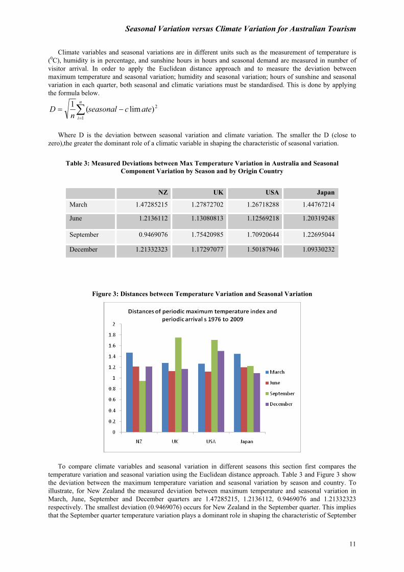
Table 3: Measured Deviations between Max Temperature Variation in Australia and Seasonal Component Variation by Season and by Origin Country

NZ UK USA Japan

March 1.47285215 1.27872702 1.26718288 1.44767214

June 1.2136112 1.13080813 1.12569218 1.20319248

September 0.9469076 1.75420985 1.70920644 1.22695044

December 1.21332323 1.17297077 1.50187946 1.09330232

Figure 3: Distances between Temperature Variation and Seasonal Variation

To compare climate variables and seasonal variation in different seasons this section first compares the temperature variation and seasonal variation using the Euclidean distance approach. Table 3 and Figure 3 show the deviation between the maximum temperature variation and seasonal variation by season and country. To illustrate, for New Zealand the measured deviation between maximum temperature and seasonal variation in March, June, September and December quarters are 1.47285215, 1.2136112, 0.9469076 and 1.21332323 respectively. The smallest deviation (0.9469076) occurs for New Zealand in the September quarter. This implies that the September quarter temperature variation plays a dominant role in shaping the characteristic of September


12

quarter seasonal variation. Low temperature and cool climate in September quarter may well have motivated New Zealanders to escape their cool season and to visit Australia. For UK and USA the smallest deviation is in the June quarter which implies that June quarter low temperature variation plays a dominant role in shaping the June quarter seasonal variation. June quarter seasonal mean values are low for the UK and USA because of low temperature in Australia and sunny and warmer climate in Northern Hemisphere. Japan has the smallest deviation in December quarter meaning that warm temperature variation in December quarter plays a dominant role in shaping the seasonal variation in December quarter. Winter in Japan and summer in Australia appears to motivate Japanese tourists to visit Australia in the December quarter.

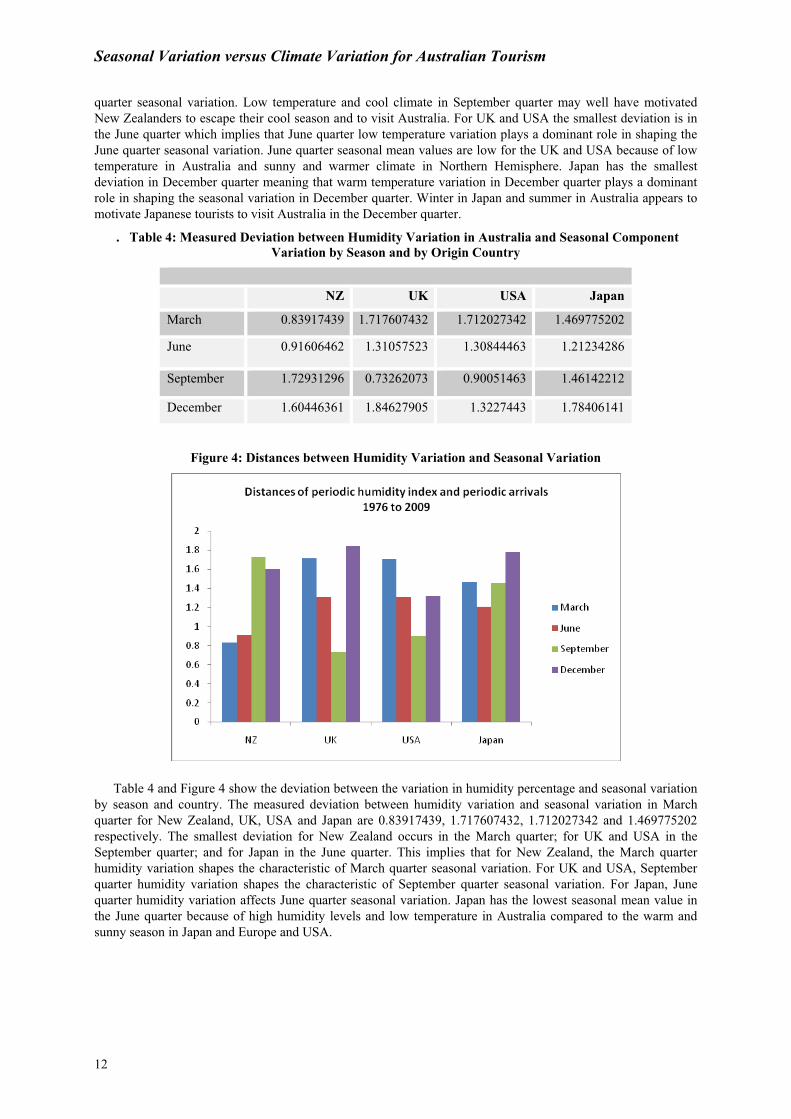
. Table 4: Measured Deviation between Humidity Variation in Australia and Seasonal Component Variation by Season and by Origin Country

NZ UK USA Japan

March 0.83917439 1.717607432 1.712027342 1.469775202

June 0.91606462 1.31057523 1.30844463 1.21234286

September 1.72931296 0.73262073 0.90051463 1.46142212

December 1.60446361 1.84627905 1.3227443 1.78406141

Figure 4: Distances between Humidity Variation and Seasonal Variation

Table 4 and Figure 4 show the deviation between the variation in humidity percentage and seasonal variation by season and country. The measured deviation between humidity variation and seasonal variation in March quarter for New Zealand, UK, USA and Japan are 0.83917439, 1.717607432, 1.712027342 and 1.469775202 respectively. The smallest deviation for New Zealand occurs in the March quarter; for UK and USA in the September quarter; and for Japan in the June quarter. This implies that for New Zealand, the March quarter humidity variation shapes the characteristic of March quarter seasonal variation. For UK and USA, September quarter humidity variation shapes the characteristic of September quarter seasonal variation. For Japan, June quarter humidity variation affects June quarter seasonal variation. Japan has the lowest seasonal mean value in the June quarter because of high humidity levels and low temperature in Australia compared to the warm and sunny season in Japan and Europe and USA.


13

Table 5: Measured Deviation between Hours of Sunshine in Australia and Seasonal Component Variation by Season and by Origin Country

NZ UK USA Japan

March 1.42958473 1.25809956 1.30600903 1.46109466

June 1.19565243 1.12165037 1.14280752 1.20875749

September 1.5489356 1.17998129 1.06822103 1.48323643

December 1.22583412 1.50169617 1.42391146 1.3695123

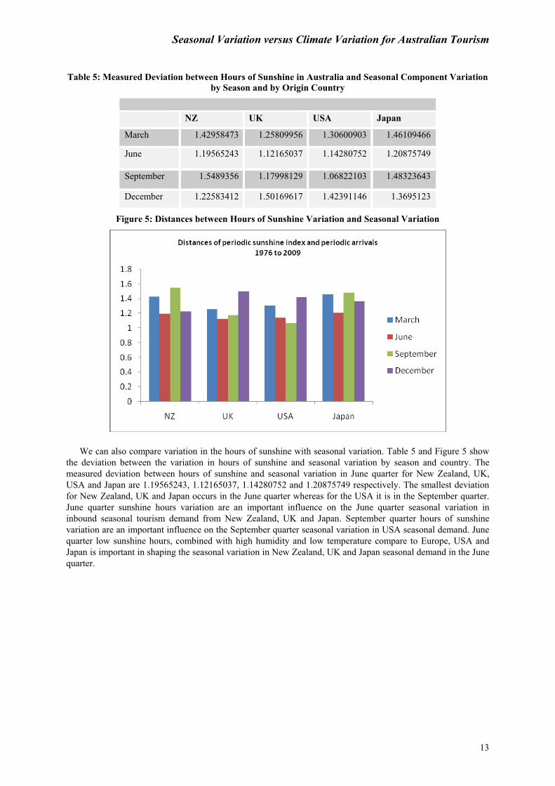
Figure 5: Distances between Hours of Sunshine Variation and Seasonal Variation

We can also compare variation in the hours of sunshine with seasonal variation. Table 5 and Figure 5 show the deviation between the variation in hours of sunshine and seasonal variation by season and country. The measured deviation between hours of sunshine and seasonal variation in June quarter for New Zealand, UK, USA and Japan are 1.19565243, 1.12165037, 1.14280752 and 1.20875749 respectively. The smallest deviation for New Zealand, UK and Japan occurs in the June quarter whereas for the USA it is in the September quarter. June quarter sunshine hours variation are an important influence on the June quarter seasonal variation in inbound seasonal tourism demand from New Zealand, UK and Japan. September quarter hours of sunshine variation are an important influence on the September quarter seasonal variation in USA seasonal demand. June quarter low sunshine hours, combined with high humidity and low temperature compare to Europe, USA and Japan is important in shaping the seasonal variation in New Zealand, UK and Japan seasonal demand in the June quarter.


14

Table 6: Quarters showing the Minimum Deviation between Climate Variation and Seasonal Variation,

for Each Origin

Climate NZ UK USA Japan Selected Highest

Frequent Quarter

Temperature Sept June June Dec June (50%)

Humidity March Sept Sept June Sept (50%)

Sunshine Hours June June Sept June June (75%)

Selected Most Frequent Quarter

Nil June (75%)

Sept (75%)

June (75%)

Table 6 summaries the quarters that have the minimum deviation from the following comparisons:

temperature variation versus seasonal variation; humidity variation versus seasonal variation; and hours of sunshine variation versus seasonal variation. A link is identified between climate variation and seasonal variation in June and September quarters for the Australian major tourism markets New Zealand, USA UK and Japan. If the Australian climatic pattern changes in June and September quarter it could change the characteristic pattern of seasonal variation in these quarters from New Zealand, USA, UK and Japan.

4. PERIODIC GROWTH IN SEASONAL VARIATION VERSUS PERIODIC GROWTH CLIMATE VARIATION BY SEASONS AND BY ORIGIN

Changes in climate variables are likely to influence the changes in seasonal variation. For example, when Australia moves from the June quarter to the September quarter or September quarter to December quarter, the seasonal variation in seasonal inbound tourism demand is more likely to change due to a warmer and sunny temperate. The Euclidean minimum distance approach was used to identify, for Australia, the link between the periodic growths in maximum temperature, hours of sunshine and humidity variation/periodic growth in seasonal variation.

Table 7: Measured Distances between Change in Temperature in Australia and Change in Seasonal Variation by Quarters and by Origin Country

NZ UK USA Japan

March 1.2787953 1.39876181 1.38740993 1.29763096

June 1.34404946 1.4679524 1.48090137 1.49987933

September 1.16234664 1.21804056 1.41487023 1.1408186

December 1.17087385 1.49213735 1.52636186 1.28671766


15

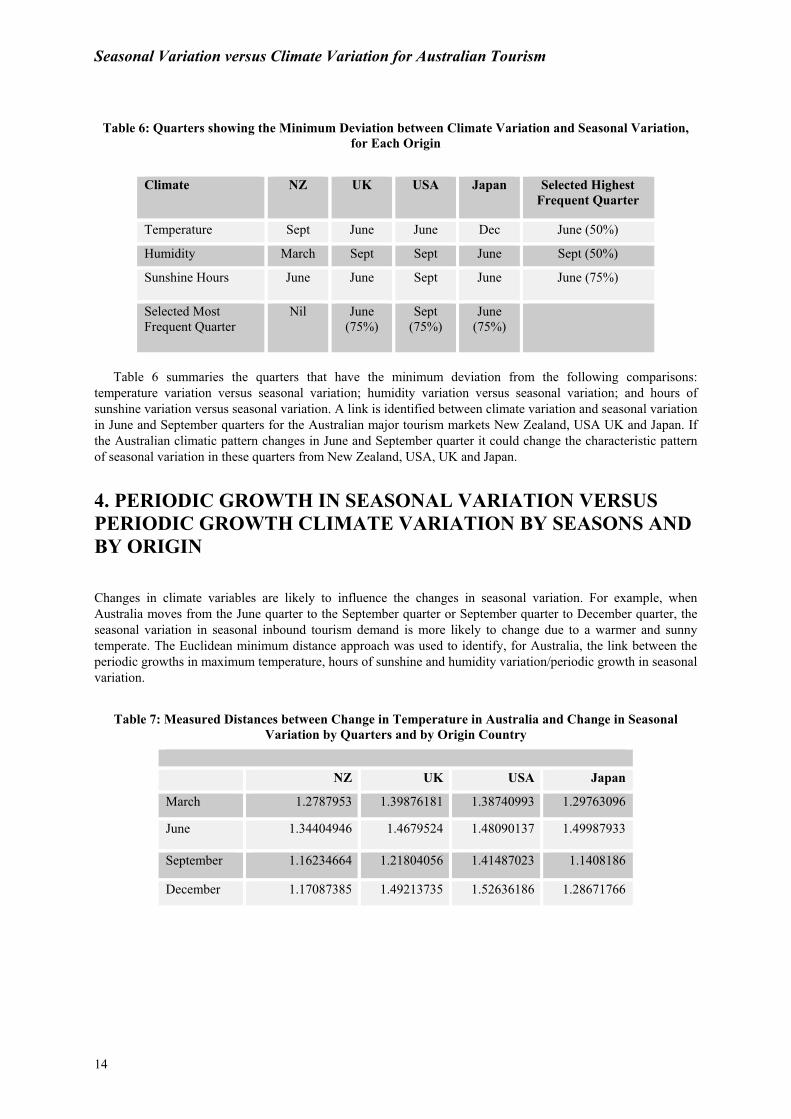
Figure 6: Distances of Periodic Change in Maximum Temperature and Periodic Change in Seasonal Variation by Quarter and Country

First, this analysis begins with comparing the growth in temperature variation and growth in growth in seasonal variation using the Euclidean method.. Table 7 and Figure 6 measured the deviation between the change in temperature variation and change in seasonal variation by season and origin country. To illustrate, the measured distance between change in temperature and change in seasonal variation from March quarter to June quarter for New Zealand, UK, USA and Japan are 1.34404946, 1.4679524, 1.48090137 and 1.49987933 respectively. For New Zealand, UK and Japan the smallest distance occur in the September quarter. For the USA it is in the March quarter. This implies that for New Zealand, UK and Japan the change in temperature from June quarter to September quarter plays a dominant role in shaping the characteristic of change in seasonal variation from June quarter to September quarter. For USA, the change in temperature from December quarter to March quarter shaping the characteristic of change in seasonal variation from December quarter to March quarter.

Table 8: Measured Distances between Change in Humidity and Change in Seasonal by Quarters and by Country

NZ UK USA Japan

March 1.50713015 1.51952236 1.30565702 1.37774994

June 1.22765229 1.23268908 1.1426535 1.17377593

September 1.41932414 1.28899927 1.57757595 1.35092093

December 1.44910646 1.27970815 1.42692407 1.17498244


16

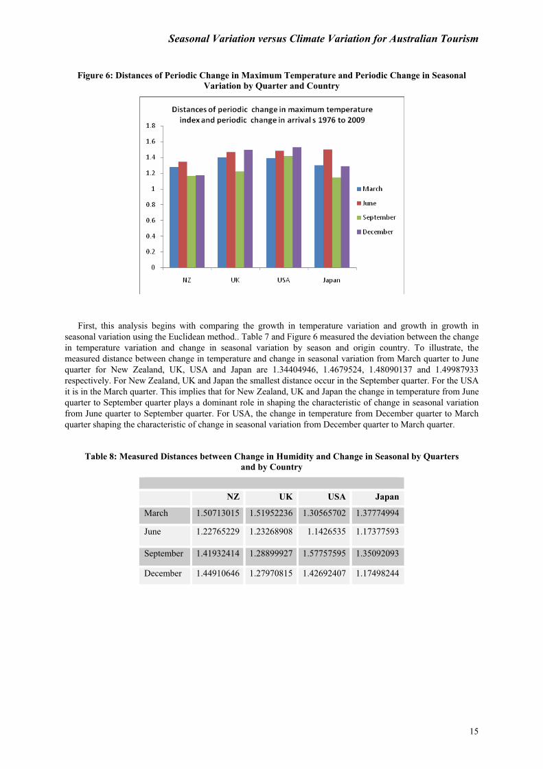
Figure 7: Distances of Periodic Change in Humidity Variation and Periodic Change in Seasonal Variation

We next compare the growth in humidity variation and growth in seasonal variation using the Euclidean method. Table 8 and Figure 7 show the deviation between the change in humidity variation and change in seasonal variation by season and country. The measured distance between change in humidity and change in seasonal variation in June quarter for New Zealand, UK, USA and Japan are 1.22765229, 1.23268908, 1.1426535 and 1.17377593 respectively. June quarter distances are the smallest distance for New Zealand, UK, USA and Japan. This implies that the change in humidity from the March quarter to the June quarter is important in shaping the characteristic of change in the seasonal variation from March quarter to June quarter. Table 2 shows that New Zealand, UK, USA and Japan, June quarter seasonal mean values reduced by 98%, 221%, 197% and 270% may be due to increased humidity levels and cool climate in Australia compared to Europe, Japan and USA.� Table 9: Measured Distance between Change in Hours in Sunshine and Change in Seasonal Variation by

Quarters and by Country

NZ UK USA Japan

March 1.46451829 1.51679696 1.16410413 1.41166069

June 1.55721914 1.19732562 1.24042131 1.24705302

September 1.24788587 1.09422375 1.11374203 1.11671528

December 1.42114741 1.25518898 1.25780925 1.309509


17

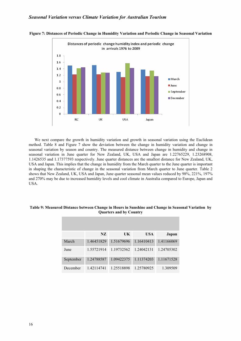
Figure 8: Distances of Periodic Change in Hours of Sunshine Variation and Periodic Changes in Seasonal Variation

Finally, we compare the growth in hours of sunshine variation and growth in seasonal variation using the Euclidean method. Table 9 and Figure 8 show the deviation between the change in hours of sunshine variation and change in seasonal variation by season and country. The measured distance between change in hours of sunshine and change in seasonal variation from June quarter to September quarter for New Zealand, UK, USA and Japan are 1.24788587, 1.09422375, 1.11374203 and 1.11671528 respectively. For New Zealand, UK, USA and Japan the smallest distance occur in the September quarter. This implies that change in hours of sunshine from the June quarter to the September is important in influencing the same period changes in seasonal variation. Table 9 shows that on average that the September quarter hours of sunshine is greater than the June quarter by 7.5% implying that more time is available in the September quarter for tourism related activity.

Table 10: The Selected Quarters from the Comparison of Periodic Change in Climate Variation and Periodic Change in Seasonal Variation

Climate NZ UK USA Japan Selected Most Frequent Quarter

Temperature Sept Sept March Sept Sept (75%)

Humidity June June June June June (100%)

Sunshine Hours Sept Sept Sept Sept Sept (100%)

Selected Most Frequent Quarter

Sept Sept (75%)

Nil Sept (75%)

Table 10 summarises the quarters that has the minimum distance in the comparisons of periodic change in

each component of the climatic variables variation and periodic change in seasonal variation. For all major high yield markets USA, UK, Japan and New Zealand the following link has been identified: change in humidity level from March quarter to June quarter is shaping the characteristic of changing the seasonal variation from March quarter to June quarter. Change in the hours of sunshine from June quarter to September quarter is shaping the characteristic of changing seasonal variation from June quarter to September quarter.


18

5. THE IMPACT OF CLIMATE VARIATION ON SEASONAL VARIATION

Seasonal variation in Australian inbound holiday seasonal demand is influenced by the climatic variables such as maximum temperature variation, humidity variation, hours of sunshine variation and institution factors includes Christmas and Easter Holiday and special events. That is:

Seasonal variation = f( maximum temperature variation, sunshine hours variation, humidity variation Easter Holiday, Christmas Holiday, special events) .

To measure the impact of maximum temperature variation, humidity variation and hours of sunshine

variation this section introduces the following regression model.

Ln(seasonal Variation) = �0 + �1D1 x T + �2D2 x T + �3D3 x T + �4ln(Max Temp) + �5ln (Humidity) + �6 ln(sunshine hours) + �7(D1) + �8(D2) + �9 (DE) + �10(Dc) + ut

Where, ut is the error term and ln is the logarithmic transformation. The dependent variable is the seasonal

variation which is measured by number of visitor arrivals. The independent variables are: maximum temperature variation measured by (0C); humidity measured in percentage; and hours of sunshine measured in hours. D1, D2 and D3 are seasonal dummy variables where D1=1 when June quarter (Jq) =1, 0 otherwise, D2=0 when September quarter (Sq) =1, 0 otherwise and D3= 1 when December quarter (Dq) =1 0 otherwise. T is the time trend. Plot 2 shows that the seasonal variation in USA, UK Japan and New Zealand holiday seasonal tourism demand exhibits an increasing seasonal variation and increasing by quarter. To model an increasing seasonal variation, seasonal dummy variables D1, D2 and D3 are multiplied by a trend component (s1=D1 x T, s2= D2 x T and s3= D3 x T, where T is the trend, D1 = Jq, D2= Sq and D3 = Dq). This method of modelling the increasing seasonal variation is based on that developed by Frances and Koehler (1998). To capture the impact of holiday periods on seasonal variation two dummy variables Easter Holiday (falls in April) dummy variable (DE= 1, when Jq=1 0 otherwise) and Christmas Holiday dummy variable (DC=1, when Dq=1 0 otherwise) were included. Two special events dummy variables were also included to represent the 2000 Olympic Games in Sydney (D1= 1, when t= Sept. 2000 and t= Dec.2000) and September 11, 2001 (D2=1, when t=Sept. 2001) incident in the United States.

OLS method cannot be used to estimate the seasonal variation regression model because the regression model error term (ut) does not have the constant error variance and exhibits the heteroskedasticity problem. The test for Autoregressive Conditional Heteroskedasticity (ARCH) effect in the error term (ut) as discussed in Maddala (2001, p.468) confirmed the ARCH effect. Therefore, to model the seasonal variation, this study considered the Autoregressive Conditional Heteroskedasticity (ARCH) modelling approach (Engle 1982). The rationale for introducing the ARCH (4) model is to add a second equation �t

2= � + �1(ut-1)2 + �2(ut-2)2 + �3(ut-3)3 + �4(ut-4) 2 to the standard regression model. The conditional variance equation plausibly depends on the squared residuals (u2

t-1. .u2t-2…). The ARCH modelling approach allows for simultaneous estimation of conditional

means and conditional variances overtime.

The above time-series model was estimated with Eviews (6.0) using the method of maximum likelihood. The estimated time-series model for USA, UK, Japan and New Zealand are presented in Table 11. The adjR2 goodness of fit and all test include F test for model validity, LM (4) test for fourth order serial correlation, DW for first order serial correlation, White test for constant error variance and JB tests for normality confirmed these estimated models are valid.


19

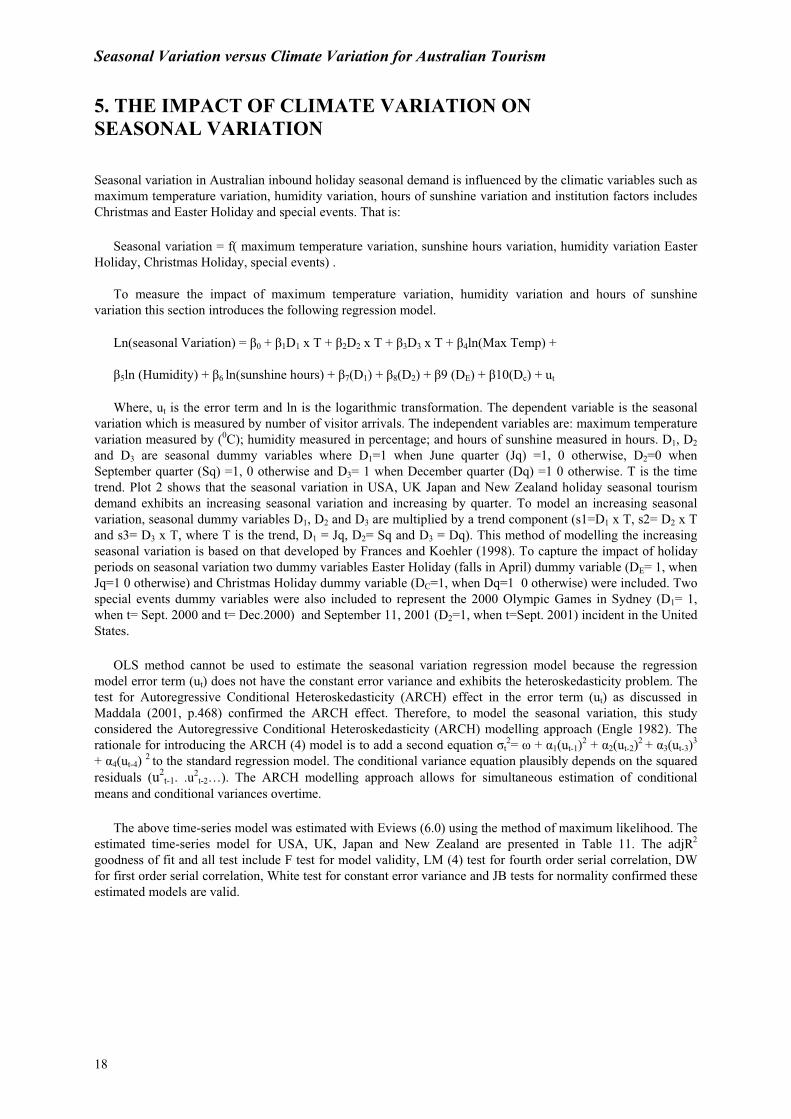
Table 11: Estimated Time Series Seasonal Variation Model

USA Ln(Seasonal) = -4.406 + 0.0006 S2 - 0.001S3 + 0.212 Dc + 1.229 LnTemp + 0.131LnHum (z= -12.7) (z=3.808) (z=-4.94) (z=9.265) (z=27.17) (z=2.149) �2 = 0.0008 + 0.052(Ut-1)2 + 0.012 (Ut-2)2 - 0.114 ( Ut-3)2 + 0.537(Ut-4)2 (z=2.575) (z=0.781) (z=0.181) (z=1.064) (z=2.88) Adj. R2=0.869 Prob. (F test) = 0.000 DW=2.431 JB(4)=2.165 LM(4)=0.831 WH(4)=0.3195 UK Ln(Seasonal) = -6.313 + 0.208 DC + 1.700 LnTemp + 0.252 LnHum (z=-27.42) (z=16.64) (z=60.18) (z=4.198) �2= 0.0006 + 0.008(Ut-1)2 + 0.026 (Ut-2)2 + 0.115 ( Ut-3)2 + 0.782(Ut-4)2 (z=0.782) (z=0.792) (z=1.618) (z=0.801) (z=4.129 ) Adj R2=0.839 Prob. (F test) = 0.000 DW=2.09 JB(4)=0.435 LM(4)=0.011 WH(4)=0.200 NZ Ln(Seasonal) =3.404 - 0.0006 S1+0.001S2+0.0006 S3+0.104DE+0.156 DC -1.314 LnTemp+ 0.306LnSun (z=23.7) (z=-4.15) (z=7.38) (z=3.45) (z=8.47) (z=8.044) (z=-31.497) (z=9.210) �2= 0.0006 -0.035(Ut-1)2 + 0.141 (Ut-2)2 + 0.075 ( Ut-3)2 + 0.666(Ut-4)2 (z=2.916) (z=-2.346) (z=1.903) (z=1.638) (z=2.932) Adj R2=0.895 Prob. (F test) = 0.000 DW=2.076 JB(4)=1.322 LM(4)=0.818 WH(4)=0.320 Japan Ln(Seasonal) = -2.713 + 0.0005S1 + 0.001S2 - 0.006 S3 + 0.547 DC + 0.849 Ln Temp (z=-19.8) (z=4.11) (z=14.05) (z=-27.6) (z=29.095) (z=20.16) �2= 0.0004 - 0.0006 (Ut-1)2 + 0.003 (Ut-2)2 - 0.001 ( Ut-3)2 + 1.174(Ut-4)2 (z=1.65) (z=-0.155) (z=0.319) (z=-0.603) (z=3.719 ) Adj R2=0.543 Prob. (F test) = 0.000 DW=2.296 JB(4)=0.513 LM(4)=0.377 WH(4)=0.156 Notes: S1= D1*T, S2= D2*T, S3 = D3*T, DE = Easter Dummy, DC=Christmas Dummy Table 12: Estimated impact of Maximum Temperature, Humidity, Sunshine Hours on Seasonal Variation

Country Temperature Humidity Sunshine Dc De

USA 1.229 0.131 0.212

UK 1.700 0.252 0.208

NZ -1.314 0.306 0.158 0.104

Japan 0.849 0.547 Note: Dc is Christmas Dummy, De is Easter Dummy

Table 12 shows the impact of maximum temperature, humidity, and sunshine hours on seasonal variation for

USA, UK, NZ and Japan. Maximum temperature has the positive sign except for NZ. A one percent (1%) increase in maximum temperature would increase the seasonal variation by 1.229%, 1.7%, and 0.849% for USA, UK and Japan respectively. A one percent (1%) increase in humidity would increase the seasonal variation by 0.131% and 0.252% for USA and UK respectively. A one percent (1%) increase in sunshine hours would increase the seasonal variation by 0.306% for NZ. Australia’s Christmas holiday has a positive impact on seasonal variation in USA, UK and Japan seasonal tourism demand, whereas Christmas and Easter holidays have positive impact on seasonal variation in New Zealand seasonal tourism demand.


20

6. CONCLUSIONS

This study has proposed a new approach to identify the relationship between climate variables such as maximum temperature, relative humidity, and hours of sunshine and seasonal variation in tourism. The context was holiday tourism to Australia from the USA, UK, Japan and New Zealand. First the seasonal component in holiday tourism to Australia was extracted using the BSM modelling approach. Secondly, the Euclidean minimum distance approach was used to measure the deviation between the climate variation and seasonal variation to identify the similarity in the pattern. The advantage of using the seasonal component is that it allows the comparison of maximum temperature, relative humidity, and hours of sunshine/seasonal variation by season. Finally, time-series modelling was considered to measures the direct impact of climate variable maximum temperature, relative humidity, and hours of sunshine on seasonal variation.

Climate variations are shaping the characteristic of seasonal variation in holiday tourism demand. The effects on seasonal variation tend to vary between season and origin countries. The minimum distance approach shows the link between temperature variation, humidity percentage variation and hours of sunshine variation/ seasonal variation in different seasons and origins. Links were identified between the temperature variation, humidity variation and sunshine hours variation/ seasonal variation for New Zealand in the September quarter, March quarter, and June quarter respectively; for the UK in the June quarter, September quarter, and December quarter respectively; for the USA the in June quarter, September quarter, and September quarter respectively; and for Japan in the December quarter, June quarter, and September quarter respectively. In Australia, June quarter climate is cool, whereas Northern Hemisphere countries include Europe, USA and Japan are warm and sunny and both share different season. June quarter low temperature, combined with high humidity level and low hours of sunshine is identified as important in shaping the characteristic pattern of the seasonal variation in UK, USA and Japan seasonal demand in the June quarter.

The link between growths in temperature variation, humidity variation and hours of sunshine variation and

seasonal variation tends to vary by season and country. For all major markets, June quarter growth in humidity variation is linked to the same quarter growth in seasonal variation. September quarter growth in hours of sunshine variation and temperature variation is linked to September quarter growth in seasonal variation.

The Autoregressive Conditional Heteroskedasticity (ARCH) modelling approach was used to measure the

impact of climate variables on the seasonal component. The overall impact of maximum temperature, humidity, and sunshine hours on seasonal variation varies by country. USA and UK seasonal variation is influenced by maximum temperature and humidity. NZ seasonal variation is influenced by maximum temperature and sunshine hours. Japan’s seasonal variation is influenced by only temperature. The estimated elasticity of maximum temperature is high for all countries which is the most important climate factor influencing seasonal variation in holiday tourism. The impact of Australian temperature on seasonal variation cannot be generalised to all tourist origin countries. Australian temperature has a positive impact on countries that share different seasons and negative impact on countries share same season.

Temperature and humidity are the important and significant determinants of seasonal variation in holiday

international tourism demand to Australia. Both warm temperature and certain humidity level create the comfortable climate condition for Australian tourist. Any reduction in humidity level due to global warming could have an adverse effect on Australian tourism. To maintain a steady growth in international seasonal tourism demand Australia should have a comfortable climate condition in most of the seasons.

Australian tourism industry is adversely affected in June and September quarters due to low seasonal

demand. June quarter seasonal demand is very low compare to September quarter. The reason for the low demand is that during these periods Australia is in cool season whereas its major high yield markets USA, UK and Japan are in warm and sunny season. To increase the June and September quarters visitor arrivals from major high spending market such as USA, UK and Japan Tourism Australia should work closely with hotel industry, travel industry, government and states/territories to develop a strategic plan. This can be achieved from the development of low cost package tourism. Secondly, identifying the different market segments which are not depend on climate such as senior citizen and business travellers and conferences and promote these markets


21

through appropriate marketing strategies.

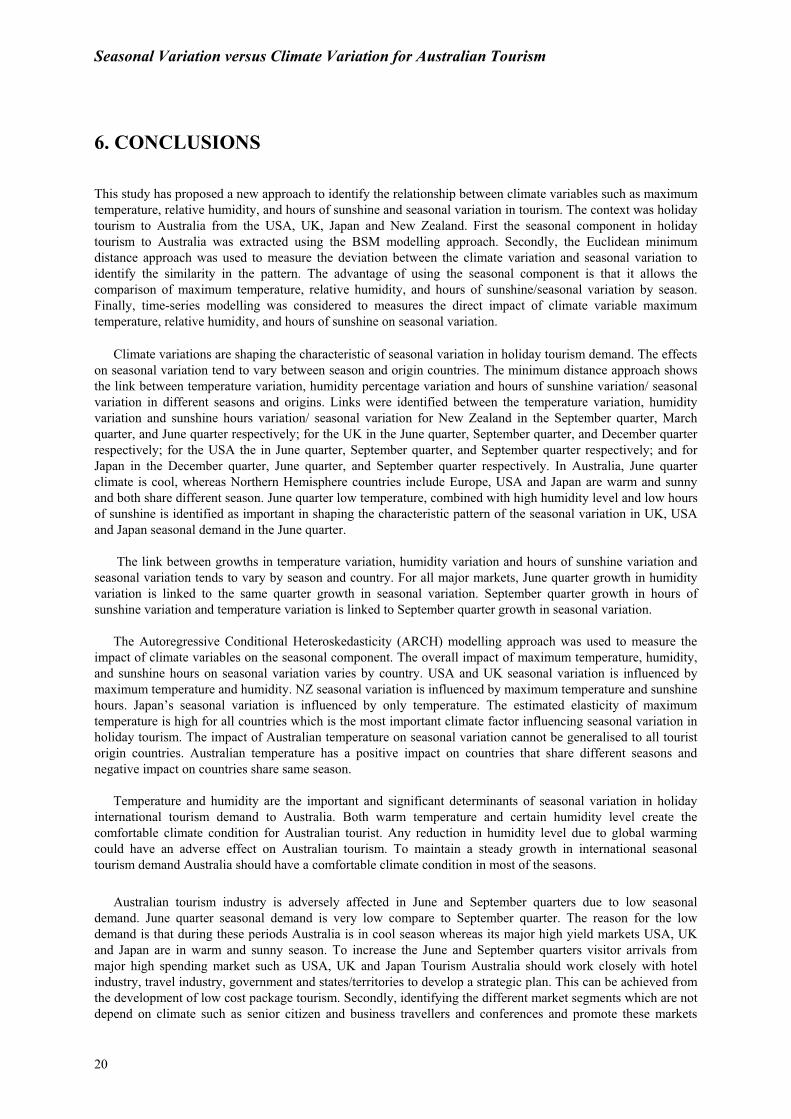
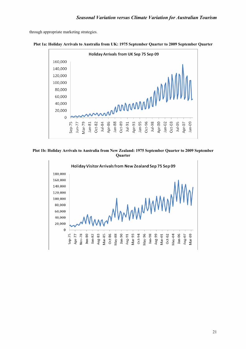
Plot 1a: Holiday Arrivals to Australia from UK: 1975 September Quarter to 2009 September Quarter

Plot 1b: Holiday Arrivals to Australia from New Zealand: 1975 September Quarter to 2009 September Quarter


22

Plot 1c: Holiday Arrivals to Australia from USA: 1975 September Quarter to September 2009 September Quarter

Plot 1d: Holiday Arrivals to Australia from Japan: 1975 September Quarter to 2009 September Quarter


23

Plot 2: Maximum Temperature, Relative Humidity and Sunshine Hours from 1975 September Quarter to 2009 September Quarter

Plot 3: Extracted Seasonal Variation from Holiday Visitor Arrivals to Australia from NZ, UK, USA and Japan Using the BSM modelling Approach from 1975 September quarter to 2009 September Quarter.


24


25


26

REFERENCES

Amelung, B. and D. Viner (2006). ‘Mediterranean Tourism: Exploring the Future with the Tourism Climatic Index’. Journal of Sustainable Tourism, Vol. 14, No.4, 349-549.

Berrittela, M., A. Bigano., R.Roson, and R.S.J. Tol (2006). ‘A general equilibrium analysis of climate change impacts on tourism’, Tourism Management, 27, 913-924.

Crouch, G.I.(1995). ‘A Meta-Analysis of Tourism Demand’ , Annals of Tourism Research, 22(1), 103-118. Crouch, G.I., L.Schultz, and P. Valerio (1992). ‘Marketing International Tourism to Australia: A Regression Analysis’.

Tourism Management, 13, 196-208. Divisekera, S. (2003). ‘ A Model of Demand for International Tourism’. Annals of Tourism Research, 30, 31-49. Dwyer, L. and C. Kim (2003). ‘Destination Competitiveness: Determinants and Indicators’, Current Issues in Tourism, vol.6,

5, 369-414. Engle, R.F.(1982). ‘Autoregressive Conditional Heteroscedasticity with Estimates of the Varaince of UK Inflation,

Econometrica, 50, 987-1007. Frances, P.H. and A.B. Koehler (1998). ‘A Model Selection Strategy for Time Series with Increasing Seasonal Variation’,

International Journal of Forecasting, 14, 405-414. Goh, C., R. Law, and H.M.K. Mok. (2008). ‘Analyzing and Forecasting Tourism Demand: A Rough Sets Approach’ Journal

of Travel Research, 46, 327-338 Gomez M.M. B. (2005). ‘Weather, Climate and Tourism’. Annals of Tourism Research, Vol. 32, No. 3, pp.571-591. Hamilton, J.M. and M.A. Lau (2004). ‘The Role of Climate Information in Tourist Destination Choice Decision-Making’ ,

Centre for Marine and Climate Research, Hamburg University, Hamburg, Germany November 25, Working paper FNU-56..

Hamilton,J.M., D.J.Maddison, and R.S.J. Tol. (2205). ‘Climate Change and International Tourism: A Simulation Study’, Global Environmental Change, 15, 253-266.

Harvey, A. C. (1989). Forecasting, Structural Time Series Models and the Kalman Filter, Cambridge University Press. Hamilton, J.M. and R.S.J. Tol. (2007). ‘The Impact of Climate Change on Tourism in Germany, the UK and Ireland: A

Simulation Study’, Regional Environmental Change, 7(3):161-172. Hylleberg, S.(1992).Modelling Seasonality. Oxford University Press, Oxford OX2 6DP. IPCC (2007) Intergovernmental Panel on Climate Change (IPCC) Climate Change 2007: Synthesis Report, An

Assessment of the Intergovernmental Panel on Climate Change, December 2007, http://www.ipcc.ch/ipccreports/ar4-syr.htm.

Koenig-Lewis N.and E. Bischoff (2005) Seasonality research: the state of the art International Journal of Tourism Research Volume 7 Issue 4-5, Pages 201 - 219

Kulendran, N. (1996). ‘Modelling Quarterly Tourist Flows to Australia Using Cointegration Analysis’. Tourism Economics,

2, 203-222. Kulendtran, N.and S. Divisekera (2007). ‘Measuring the Economic Impact of Australian Tourism Marketing Expenditure’.

Tourism Economics, 13, 2, 261-274. Kulendran, N. and L. Dwyer, (2009). ‘Measuring the Return from Australian Tourism Marketing Expenditure’ Journal of

Travel Research, 47, 3, 275-284. Lim, C. and M. McAleer. (2001). ‘Monthly Seasonal Variations: Asian Tourism to Australia.’ Annals of Tourism Research,

28: 68-82. Lim, C.( 2006), ‘A Survey of Tourism Demand Modelling Practice: Issues and Implications’, in Larry Dwyer and P. Forsyth

Eds. , International Handbook on the Economics of Tourism, Edward Elgar. Lise, W. and R.S.J. Toll. (2002) ‘Impact of Climate on Tourist Demand’ Climate Change, 55:429-449. Matzarakis, A. (2001a) ‘Assessing Climate for Tourism Purpose: Existing methods and Tools for the Thermal Complex’,

First International Workshop on Climate, Tourism and Recreation, Halkidiki, Greece. Matzarakis, A. (2001b) ‘Climate and Bioclimate Information for Tourism in Greece’, First International Workshop on

Climate, Tourism and Recreation, Halkidiki, Greece. Mieczkowski, Z. (1985). ‘The Tourism Climate Index: A Methods of Evaluating World Climates for Tourism’, Canadian

Geographer, 29, 3, 220-233. Jaume Rossello, N., A.R. Font. and A.S. Rossello. (2004). The Economic Determinant of Seasonal Pattern, Annals of

Tourism Research, 31(3) 697-711. Skinner, C.J. and R.J. De Dear. (2001),’ Climate and Tourism –an Australian perspective’, First International workshop on

climate, Tourism and Recreation, Halkidiki, Greece.


27

Stern H., G. Hoedt. And J. Ernst. (2000). ‘Objective Classification of Australian Climates’, Australian Meteorological Magazine, 49:87-96.

Stern,N., (2008). ‘The Economics of Climate Change’, American Economic Review: Papers & Proceeding, 1-37. Taylor, C., and R.A. Ortiz (2009), ‘Impacts of Climate Change on Domestic Tourism in the UK: A Panel Data Estimation’.

Tourism Economics, 15(4):803-812. Witt, S.F., and C.A.Witt. (1995). ‘Forecasting tourism demand: A review of empirical research.’ International Journal of

Forecasting, 11: 447-475

Seasonal Variation versus Climate variation for Australian Tourism · 2010-10-11 · Seasonal...

Documents

Transcript of Seasonal Variation versus Climate variation for Australian Tourism · 2010-10-11 · Seasonal...