SEASONAL UNDERGROUND THERMAL ENERGY STORAGE USING …

SEASONAL UNDERGROUND THERMAL ENERGY STORAGE

USING SMART THERMOSIPHON ARRAYS

by

Philip Martin Jankovich

A dissertation submitted to the faculty of

The University of Utah in partial fulfillment of the requirements for the degree of

Doctor of Philosophy

Department of Mechanical Engineering

The University of Utah

August 2012

T h e U n i v e r s i t y o f U t a h G r a d u a t e S c h o o l

STATEMENT OF DISSERTATION APPROVAL

The dissertation of Philip Martin Jankovich

has been approved by the following supervisory committee members:

Kent S. Udell , Chair 6/11/2012 Date Approved

Timothy Ameel , Member 6/8/2012

Date Approved

Eric Pardyjak , Member 6/8/2012

Kuan Chen , Member 6/16/2012

Date Approved

Greg Owens , Member 6/11/2012

Date Approved

and by Timothy Ameel , Chair of

the Department of Mechanical Engineering

and by Charles A. Wight, Dean of The Graduate School.

ABSTRACT

With oil prices high, and energy prices generally increasing, the pursuit of more

economical and less polluting methods of climate control has led to the development of

seasonal underground thermal energy storage (UTES) using pump-assisted smart

thermosiphon arrays (STAs).

With sufficient thermal storage capacity, it is feasible to meet all air-conditioning

and heating requirements with a trivial fuel or electrical input in regions with hot

summers and cold winters. In this dissertation, it is described how STAs can provide

seasonal energy storage to meet all climate control needs. STAs are analyzed and

compared with current similar technologies.

The objective of this research was to create a methodology to design STA systems

for any cooling load in any climate. Full year simulations were performed to model the

charging and discharging processes to minimize total pipe length. The modeling results

were validated with analytical solutions and some experimental data.

The model developed was successfully able to simulate the heat transfer in and

out of the soil through thermosiphon pipes over the course of one year using actual

weather data and loads. Based on initial modeling results, a pilot-scale thermosiphon

system was implemented. A description of this system and limited temperature data is

put forth in Chapter 4.

iv

The cooling loads of three buildings in 16 locations were calculated. Four soil

types were used in each location, and a STA was modeled and optimized for each.

Chapter 5 presents the results of these design optimizations. Optimum pipe spacing was

found to be proportional to the square root of thermal diffusivity. This correlation allows

for the development of an optimization routine that can find the optimized design faster,

which should lead to further design correlations. The total pipe length needed was found

to correlate with the thermal effusivity of the soil.

CONTENTS

ABSTRACT ....................................................................................................................... iii

LIST OF TABLES ............................................................................................................ vii

LIST OF FIGURES ......................................................................................................... viii

CHAPTERS

1. INTRODUCTION ...........................................................................................................1

Thermal Energy Storage ...................................................................................................3 Smart Thermosiphons ....................................................................................................12 Smart Thermosiphon Arrays ..........................................................................................14 Research Objectives .......................................................................................................15 References ......................................................................................................................18

2. COMSOL MODELS .....................................................................................................21

Methods ..........................................................................................................................22 Results ............................................................................................................................32 Discussion ......................................................................................................................34 Conclusions ....................................................................................................................39 References ......................................................................................................................40

3. MODELING FREEZING AND MELTING .................................................................41

Methods ..........................................................................................................................41 Results ............................................................................................................................48 MATLAB Design Methodology ....................................................................................55 References ......................................................................................................................62

4. PILOT SCALE...............................................................................................................63

Methods ..........................................................................................................................63 Discussion ......................................................................................................................69 Soil Analysis ..................................................................................................................72 Power Requirements ......................................................................................................78 References ......................................................................................................................79

vi

5. DESIGN OPTIMIZATION RESULTS .........................................................................81

Methods ..........................................................................................................................81 Results ............................................................................................................................91 Conclusion ......................................................................................................................98 References ......................................................................................................................98

6. CONCLUSIONS AND RECOMMENDED WORK ..................................................100

COMSOL Model ..........................................................................................................100 Pilot Scale .....................................................................................................................102 MATLAB Model ..........................................................................................................103 Design Optimization ....................................................................................................104 Future Work .................................................................................................................106 Final Conclusions .........................................................................................................107

APPENDICES

A. DESIGN ......................................................................................................................108

B. ANALYTICAL SOLUTIONS ....................................................................................116

C. SIMULATION CODE ................................................................................................123

D. OPTIMIZATION CODE ............................................................................................128

LIST OF TABLES

Table Page

2.1. Results of optimization study………………………………………….. 35

3.1. Temperature boundary condition modeled……………………………. 50

3.2. Physical parameters for melting due to a line source………………….. 53

4.1. Density and specific heat of various soil components………………… 74

4.2. Pilot scale soil properties by depth…………………………………….. 78

5.1. ASHRAE 90.1-2007 envelope requirements (U-values in W/m2/K)….. 86

5.2. ASHRAE 90.1-2007 envelope requirements (U-values in Btu/h/ft2/°F).…………………………………………………….……...

86

5.3. Weather file locations and climatic data (SI units)……………………. 87

5.4. Climatic data (IP units)………………………………………………... 87

5.5. Building loads (SI units)………………………………………………. 89

5.6. Building loads (IP units)………………………………………………. 90

5.7. Selected soil thermal properties (SI units)…………………………….. 91

5.8. Selected soil thermal properties (IP units)…………………………….. 91

5.9. Optimization results for building 1……………………………………. 92



5.12. Thermal effusivities……………………………………………………. 97

LIST OF FIGURES

Figure Page

1.1. Heat transfer cancellation at top of U-tube borehole heat exchangers… 5

1.2. The operation of a heat pipe.…………………………………………... 8

1.3. The operation of a thermosiphon, or gravity-assisted heat pipe………. 9

1.4. Thermosiphon operating in pump-assisted mode……………………… 11

2.1. Circular 7-pipe domain. Dimensions in meters……………………….. 23

2.2. Domain modeled representing infinite square matrix. Dimensions in meters…………………………………………………………………..

23

2.3. Square matrix domain showing thermosiphon pipes and domain modeled………………………………………………………………...

24

2.4. Thermal conductivity, k, as a function of temperature, T……………... 26

2.5. Specific heat as a function of temperature indicating the strong spike due to the phase change at 273.15 K…………………………………...

27

2.6. Empirical model of annual temperatures……………………………… 31

2.7. Total energy flux out of the ground during winter…………………….. 31

2.8. Results from COMSOL study…………………………………………. 33

2.9. Half-year heat fluxes…………………………………………………... 36

3.1. General model geometry with even node spacing to N nodes………… 44

3.2. Modeled melt radius R(t) and λt compared to closed-form solution…... 55

3.3. Geometry of hexagonal array, showing area not modeled (Alost) by chosen method………………………………………………….............

57

ix

3.4. Increased node spacing based on consecutive sums…………………... 60

4.1. Arrangement of seven thermosiphon pipes for pilot scale…………… 64

4.2. Direct-push drilling, using a pneumatic hammer and expendable tip…. 65

4.3. Thermosiphon pipes installed………………………………………….. 65

4.4. Thermosiphons with heat exchangers…………………………………. 66

4.5. Float switch and pump assembly……………………………………… 67

4.6. Pipe connectivity at top of thermosiphon pipe………………………… 68

4.7. Underground temperature profile……………………………………… 69

4.8. Infrared image of heat exchanger……………………………………… 70

5.1. Number of pipes associated with 1, 2, and 3 hexagons………………... 95

5.2. Correlation between diffusivity and separation……………………….. 97

CHAPTER 1

INTRODUCTION

Due to increasing energy costs, pollution, awareness of global climate change,

and concern over the negative geopolitical consequences of reliance on foreign oil, there

is more focus on energy conservation and sustainability. Economically, it makes sense to

have technologies that consume less energy and offset demand for power from daytime

peak hours. Environmentally, technologies that pollute less and generate fewer

greenhouse gases, including carbon dioxide, are gaining favor when costs can be

controlled.

Approximately one quarter of the carbon dioxide the United States produces is

from burning fossil fuels to meet residential energy needs, mostly for heating and air

conditioning [1]. It is also known that conservation produces the greatest decrease in

carbon dioxide production per dollar spent [2]. It follows that the least expensive way to

reduce residential carbon dioxide emissions is through improved climate control

efficiencies.

According to the latest report of electricity consumption published by the Energy

Information Administration (EIA), 41% of electricity consumed in commercial buildings

goes toward space heating, ventilation, cooling, and refrigeration. Cooling is the second

largest end-use for electricity in commercial buildings [3]. As more data centers and

server rooms are built, and temperatures increase from global warming, the cooling load

2

for buildings increases. The increasing cooling load is partially indicated by the increase

in residences cooled by air conditioners from 64% in 1993 to 87% in 2009 [4-5]. To

alleviate the power consumed by air conditioning and other cooling equipment, new

technologies need to be developed that can handle the load without consuming as much

power.

There are many opportunities for conservation in space cooling. Some of the

popular methods in practice include two stage evaporative cooling, ground source heat

pumps, daily thermal energy storage, hybrid systems, demand control, and better building

envelopes. In climates with hot summers and cold winters, it is thermodynamically

possible to provide all heating and air-conditioning needs, without significant fuel or

electrical energy input, by storing heat or “cold” for use during the opposite season; this

is called seasonal thermal energy storage.

Seasonal thermal energy storage (STES) has three principal obstacles:

1. A large amount of storage medium must be available with the heat capacity to

satisfy the integrated load of an entire season.

2. An effective method of transferring heat in and out of the storage medium must be

designed to handle peak loads and charge rapidly when the opportunity arises.

3. There is potential for large thermal losses due to the inherent temperature

difference between the storage medium and its surroundings during discharge.

If the heat transfer and storage problems can be solved, there is great potential for

energy savings and CO2 reductions using seasonal thermal energy storage. As such,

seasonal thermal energy storage heating and cooling could be able to provide zero-carbon

heating and air conditioning.

3

This dissertation details the use of a new technology, smart thermosiphon arrays

(STAs), to transfer heat to and from soils effectively. Based on preliminary analysis,

computer models, and experimental data, it is clear that these systems exchange adequate

thermal energy with the ground to provide all the cooling needs of a typical house or

business, with minimal electrical or fossil fuel energy input. The goal of this research was

to understand the parameter effects associated with thermosiphon arrays to further the

engineering knowledge toward the design of a 100% carbon-free heating and cooling

system indistinguishable in simplicity and comfort from conventional heating,

ventilation, and air-conditioning (HVAC) systems.

Thermal Energy Storage

Technologies that store thermal energy for future use can be divided into three

primary categories. These are sensible heat storage (specific heat), latent energy storage

(phase change materials), and thermochemical (including nuclear) storage [2]. The most

common examples of thermal energy storage use geologic materials such as rock, soils,

or concrete to store sensible energy and water to store latent energy [6]. The amount of

sensible energy stored in these materials depends on their heat capacity, volume, and

temperature. The amount of latent energy stored depends on the fraction of phase change

material and the heat of fusion or vaporization. Some of the existing thermal energy

storage systems are reviewed in [7].

Geologic material is considered in this research as the heat storage medium

because of its availability, low cost, lack of size restrictions, adequate thermal capacity,

and low conductivity. This solves the first obstacle of STES, providing a relatively semi-

4

infinite storage medium. When using the soil as the storage medium, it is more

specifically called underground thermal energy storage (UTES).

When soil is used as the energy storage medium, there are only a few restrictions

on storage volume, such as drilling depth, maintenance of surface ecology, and plot size

[1,8-10]. If heated and cooled in an optimum way, soils not only buffer short-term

fluctuations in supply and demand, but also can accommodate a complete annual

heating/cooling load and serve a seasonal balancing function. Energy storage directly in

the soil also reduces the cost sensitivity of reservoir depth on optimum capacity selection

since excavation is unnecessary. So, the storage system can be easily sized to maximum

expected load by a simple increase of depth in most cases.

Ground Source Heat Pumps

The most widely used method of yearly energy storage currently is ground source

heat pumps (GSHPs) that use ground loop heat exchangers (GLHEs) to extract or inject

heat into the ground. While saving most users significant amount of money in

operational costs, these systems are not passive and, for small to medium applications,

usually have a high installation cost compared to conventional systems. These costs for

GSHPs and GLHEs are associated with a large amount of drilling, the installation of long

pipes that make up the ground loops and the compressors and pumps that move the

working fluid.

Underground thermal storage requires some kind of heat exchange with the

ground. GSHPs are some of the most widely used technologies that have heat exchange

with the ground. GLHEs used with GSHPs have been implemented in many ways.

Some of the more common methods are shown in [8]. These include pipe systems where

5

a working fluid is pumped through the pipes, generally in a closed loop. These closed

loops can be installed horizontally in trenches, vertically in boreholes, or submerged in

water bodies. Open loops can also be used with production and injection wells.

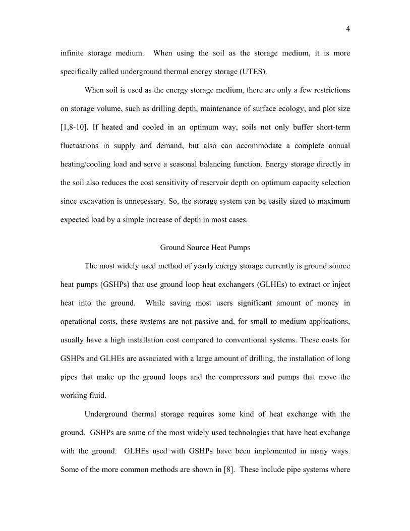
Some of the limitations of these heat exchangers are the space they take up

(horizontal loops), ineffective heat exchange due to cancellation in closely spaced pipes

(vertical loops, see Fig. 1.1) [11], or the need for a high water table and associated water

rights permits (open loops). Another recently developed method uses a self-propelled

flexible drill-head, which allows pipe to be separated sufficiently to avoid thermal

interference. This method settles the issue of cancellation, but it still requires a vapor-

compression refrigeration cycle and circulation pumps, consuming electricity [12]. All of

these limitations could be resolved with smart thermosiphons.

Figure 1.1. Heat transfer cancellation at top of u-tube borehole heat exchangers.

6

The use of smart thermosiphons is similar to u-tube boreholes, typically installed

with GSHPs, in that they facilitate heat transfer to and from the soils. Passive

thermosiphons have been used in various other applications [13]. However, rather than

heating or cooling the soil for future energy use, ground source heat pumps generally take

advantage of the earth’s relatively constant temperature [14]. Thus, energy dissipation,

rather than storage, is desired with GSHPs. In contrast, STAs are being developed to

concentrate energy for seasonal storage.

When plastic pipes are used in heat pump systems to exchange heat with the soil,

the generally accepted assumption of negligible thermal effects in plastic pipes may not

be an accurate representation of the thermodynamic coupling with the ground. Plastic

(PVC and Polyethylene) pipes were introduced for economic reasons, justified by the

argument that resistance to heat transfer is much greater in the soil than in the pipe.

However, in [15], it is shown that heat flows are substantially reduced (nearly half) due to

high thermal resistance of the pipe walls and contact resistance between pipe and soil.

Also, for vertical boreholes with closed loop tubing, “short circuiting” of heat from the

hot tube to the adjacent cold tube decreases the amount of heat that can be transferred to

the soil (see Fig. 1.1) [11,16-17]. This problem worsens as the tube spacing decreases.

The installation cost for vertical borehole installation is also high, requiring dozens of

large diameter (>0.2 m, >8 in.) boreholes to be drilled to depth for loop insertions. In

such commercial installations, an improvement in the heat transfer between the ground

and the heated space is of great importance and enormous potential economic value.

Application of smart thermosiphons, as a means of coupling heat pumps with the ground,

seems to be a simple and effective step forward.

7

A GSHP system can be replaced with a mostly passive thermosiphon system,

which uses much more effective phase change phenomena for capturing/releasing heat

[18]. If plastic u-tube piping in the ground is replaced with an array of thermosiphons

and connected directly to a heat exchanger in the heated or cooled space, there would be

no need for intermediary heat transfer fluids and heat exchangers used in GSHP systems.

Heat in a thermosiphon-based system can be transferred to and from soil to heated or

cooled medium without a vapor-compression cycle heat pump with its electrical energy

consuming compressor, intermediary heat exchangers, or liquid pumps to move water-

glycol solution through the plastic piping in the ground.

As shown in this study, thermosiphon-assisted UTES promises to meet air-

conditioning loads with under half of the drilling and pipe length used in GSHP systems.

This technology uses conventional passive thermosiphons to transfer energy out of soil

and controlled rate transfer of energy into the soil.

Heat Pipes

Heat pipes are devices that transfer heat efficiently from a region of high

temperature to a region of relative low temperature. Thermosiphons are often called

gravity-assisted heat pipes. The classical heat pipe is comprised of a closed pipe with a

wicking material on the inner surface charged with a pure working fluid. The working

fluid has to be pure in order to have effective mass transfer. The working fluid is in two

phases: vapor and liquid. The liquid is primarily contained in the wicking material.

Because of the temperature difference between the two ends of the pipe, the working

fluid, or refrigerant, evaporates on the hotter end and the vapor travels to the cooler end.

Thermodynamically, the cooler end has a lower pressure, and the saturation pressure at

8

that temperature and flow in the vapor phase are driven by the pressure difference. The

liquid phase has a capillary pressure in the wicking material that pulls it toward the

warmer end. As the working fluid condenses on the cooler side and evaporates on the

hotter side, heat is transferred efficiently from hot to cold [19], as illustrated in Fig. 1.2.

Heat pipes are primarily used in energy recovery ventilation (ERV) applications when a

contaminated airstream is exchanging heat with ventilation air, and cross-contamination

is to be avoided. Thermosiphons are a particular application of heat pipes to transfer heat

in only one direction.

Figure 1.2. The operation of a heat pipe.

9

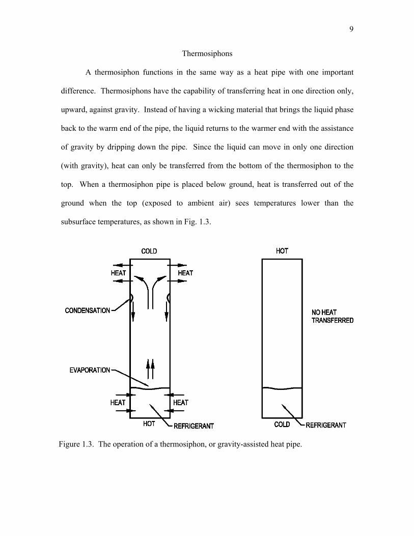
Thermosiphons A thermosiphon functions in the same way as a heat pipe with one important

difference. Thermosiphons have the capability of transferring heat in one direction only,

upward, against gravity. Instead of having a wicking material that brings the liquid phase

back to the warm end of the pipe, the liquid returns to the warmer end with the assistance

of gravity by dripping down the pipe. Since the liquid can move in only one direction

(with gravity), heat can only be transferred from the bottom of the thermosiphon to the

top. When a thermosiphon pipe is placed below ground, heat is transferred out of the

ground when the top (exposed to ambient air) sees temperatures lower than the

subsurface temperatures, as shown in Fig. 1.3.

Figure 1.3. The operation of a thermosiphon, or gravity-assisted heat pipe.

10

Conventional thermosiphon technology uses a working fluid at its saturation point

to transfer thermal energy from one end of a sealed pipe to the other [20]. When oriented

in a vertical position, the working fluid vapor will condense at the top of the pipe if the

temperature at the top is lower than the temperature at the bottom of the pipe. Upon

condensing, the fluid gives up its latent energy to the surroundings, and, assisted by

gravity, runs down the inner pipe wall to the bottom. In order to maintain pressure, more

of the liquid vaporizes from the bottom, and in doing so, takes its latent energy from the

surroundings. The overall net effect is that heat is transferred from the bottom of the pipe

to the top of the pipe when the temperature is lower at the top. No heat is transferred

when the low temperature is at the bottom (Fig. 1.3). Thermosiphons, or gravity-assisted

heat pipes, have been implemented in a variety of applications from maintaining the

permafrost in Alaska to cooling CPUs in computers [21,22].

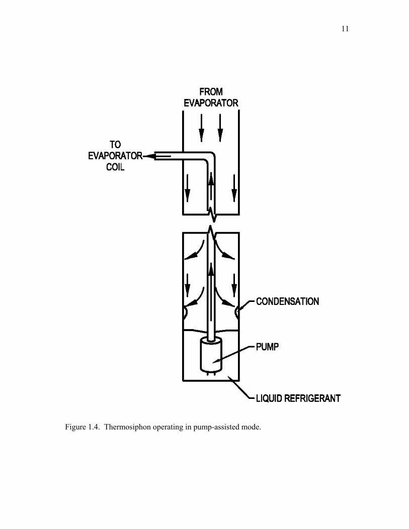
In order to reverse the process, the thermosiphon needs to be pump assisted. A

small pump located at the bottom of the pipe moves liquid to a heat exchanger located

above ground. The liquid vaporizes there and moves back to the bottom of the well as

vapor where it condenses again. This controlled mode of operation uses the ground as a

thermal sink, shown in Fig. 1.4.

During the winter season, a set of thermosiphons can be arranged to passively

freeze a subsurface section of ground large enough to meet the air conditioning needs of

the summer. The depth of these heat pipe wells should nearly equal the horizontal

distance that they cover in order to maximize the volume to surface area ratio and

minimize undesired heat losses or gains.

11

Figure 1.4. Thermosiphon operating in pump-assisted mode.

12

Smart Thermosiphons

During the summer, when there is a demand for cooling, the energy storage

system, i.e., the cold ground, can be discharged by running a thermosiphon in a pump-

assisted mode. This is a new application of thermosiphons and has not been previously

reported in the literature. A small pump placed in the bottom of a thermosiphon with a

tube attached is activated when cooling is needed (Fig. 1.4). The pump removes liquid

refrigerant from the bottom of the thermosiphon pipe and transfers it through tubing to

the surface where it can be pumped to evaporator coils. The refrigerant evaporates there

as it takes heat from its surroundings and returns to the thermosiphon in the vapor phase.

The vapor will condense on the coldest part of the pipe wall, which will be in the ground

if the ground is frozen from wintertime operation. This will drip back to the bottom

where it can be picked up by the pump again. Thus, heat is transferred from the load to

the ground.

Passive Soil-Cooling Mode

The two-phase thermosiphon considered for system performance improvement

operates on a simple heat pipe principle. Heat from the soil vaporizes the thermosiphon’s

working fluid inside of the sealed pipe. The resulting vapor moves up and carries its

latent heat to the heat exchanger where it condenses as heat is removed. That heat

exchanger would be placed in the cold winter air if the intent is to cool the soil for future

use as an air conditioning heat sink, or, if taking energy from hot soils for winter heat, in

the HVAC ducting to heat air. The condensate liquid then drains back down the

13

thermosiphon and repeats the cycle. Soil and water near the thermosiphon cool down,

giving up their thermal energy.

It should be noted that the above-described passive mode of operation for space

heating would work satisfactorily only if soil is heated in summer to above 25-28°C (77-

82°F). If soil temperature drops below 24-25°C (75-77°F), there will be a need for a

small “booster” heat pump in order to supply the room heat exchanger with the working

fluid saturated vapor at approximately 30-35°C (86-95°F).

Smart Soil-Heating Mode

Cooling of space can be achieved by reversing the working fluid flow direction in

the system. In this case, the smart thermosiphon returns liquid from the bottom of each

thermosiphon to the evaporator heat exchanger. Depending on the application (heat

rejection to chilled soil in the summer or heating of soil for future winter heating), the

evaporator would be different. For air-cooling purposes, the evaporator might be identical

to the heat exchangers found in millions of homes using vapor compression central air

conditioning. As in current residential installations, the liquid phase flows to the heat

exchanger, and the vapor leaves to be re-condensed. With chilled soils and smart

thermosiphons in place, the outside air-cooled condensing units would be eliminated (as

would their electrical load and their noise). Vapor would thus move from the air-

conditioned space to the chilled walls of the thermosiphon, giving up its heat to the

surrounding soil as it condenses. The smart thermosiphon returns liquid condensate to the

heat exchanger at a rate determined by the mass flow rate of vapor entering the

thermosiphon.

14

In the soil-heating mode, natural convection is expected in permeable soils

outside of the thermosiphon walls enhancing heat transfer. In the case of soil heated

during the summer to be used for heating in the winter, solar thermal collectors or heat

exchangers collecting process waste heat can be used. It may be possible to increase the

thermosiphon wall temperature to over 100°C (212°F), initiating water “boiling” on the

outside wall of the thermosiphon. If the water vaporized on the wall is replenished by

capillary action in the soil, an extremely effective heat transfer phenomena called the heat

pipe effect [23] can be exploited to overcome near-wall heat transfer limits.

The cooling load (especially in southern United States) is normally higher than

the heating load. If sufficient heat is removed from the soil in winter, then underground

thermal storage can become an excellent way to create an energy sink for summer.

Smart Thermosiphon Arrays

To concentrate energy in the soil for both heating and air conditioning purposes,

two STAs would be needed: one to create a “cold bank” in the winter for summer air

conditioning and the other to create a “hot bank” during the summer for winter heating. A

single array cannot be used for both purposes at the same time because the heating array

has to maintain temperatures above the conditioned space temperature all year, and the

cooling array has to maintain temperatures below. Placing the two arrays in close

proximity would create high thermal gradients and, in effect, would cancel each other

out. Arrays of smart thermosiphons are required to increase the thermal efficiency of

storage; a single thermosiphon does not allow storage since the gains in one season are

dissipated before the next season arrives. An array of thermosiphons increases the

volume of storage material to surface area of the boundary ratio. Thermal losses occur at

15

the boundary of the storage media; therefore, the surface area and the thermal gradient of

the boundary should be minimized for greatest performance.

Heating with thermosiphon arrays is not included in this research. In a well-

insulated building with process loads, plug loads, lights, and people, the internal heat

gains increase the conditioned space temperature without the assistance of a heating

system; therefore, heating is not usually required until the outdoor air temperature is 3-

6°C (5-10°F) below the desired indoor air temperature. Because of this temperature

difference between outdoor and indoor air temperature, any location with a significant

heating load has an average annual air temperature below the desired conditioned space

temperature. The average subterranean ground temperature, which is equal to the

average annual air temperature (without any geothermal or other heat sources), is the

starting point for a thermosiphon array. To use a thermosiphon array for heating, the

ground must be heated above the temperature required by the conditioned space; whereas

for cooling, the ground typically starts at a temperature below conditioned space

temperatures, making cooling easier to implement with thermosiphon arrays than heating.

In addition, freezing the soil for a cooling application inhibits fluid flow, making the

stored temperatures less likely to dissipate due to convection or other transport

phenomena.

Research Objectives

The objective of the research leading to this dissertation was to create a

methodology to design STA systems, installed in a phase change material (PCM), used

for satisfying cooling loads. The methodology is needed because of the complexity of

the systems and the variability in each application. Full-year simulations are required to

16

model the charging and discharging process, with the goal to find the minimum amount

of thermosiphon pipe to be installed that will meet the load satisfactorily. In developing

the full-year simulation, it is necessary to validate the results with known analytical

solutions and experimental data. Further research may lead to a methodology that will

approximate optimized solutions without the need to model the system iteratively.

In an effort to simulate the system accurately, the development of the theory used

in the model, including the assumptions, is required. The problem, with all of its

complexities, needs to be simplified as much as possible without losing accuracy. This

theory and subsequent simplification is presented in Chapter 2. The equations to be

solved are shown along with the assumptions and neglected effects.

The possibility of using packaged multiphysics software was explored. The

results from this research are presented in Chapter 2. Through an optimization effort in

COMSOL 3.3, it was found that packaged heat transfer software often lacks the

capability of seamlessly modeling phase change processes. Although reasonable results

were obtained, instabilities from the discontinuities in thermal properties at the phase

change, the cost of the software, the time-intensive process, the inability to use actual

weather data, and the difficulty to set up batch processes with an optimization routine

necessitated abandonment of this method. The COMSOL optimization did provide

assistance to the design of an installed pilot scale system, described in Chapter 4.

Once packaged heat transfer software was abandoned for the development of

original code, it became necessary to verify the simulation with known analytical

solutions. Few solutions exist for freezing and melting in a radial geometry. One of

these solutions is presented, as it is found in literature, along with the Stefan formulation,

17

in Appendix B. This solution is presented in its entirety because it can be used to predict,

a priori, how long a sample of phase change material will take to freeze or melt if an

adequate heat flux can be determined for the thermosiphon pipe wall. The solution also

serves as validation for the simulation code developed as part of this research.

The equations to be solved need to be formulated for discrete sections, or nodes,

of the domain to be modeled. The discretization of those equations and the process by

which the model calculates the equations is presented in Chapter 3. This development

was done to be able to model the heat transfer in and out of the soil over the course of one

year to determine if a particular design of STAs is adequate for a particular cooling load.

The model was created in MATLAB and validated through comparisons with three

analytical solutions. These comparisons are presented in Chapter 3. The three analytical

solutions, in radial coordinates, include the steady-state solution of temperature boundary

conditions at the inner and outer radii (without phase change), the time to change phases

with a flux boundary condition at the inner radius, and the flux boundary condition with a

moving front, which is the solution presented in Appendix B. All three analytical

solutions validate the model.

In order to use the simulation model for the design and optimization of

thermosiphon arrays, some constraints, assumptions, and input parameters are necessary.

Chapter 3 presents the constraints to geometry, the weather files to be used as boundary

conditions, and the determination of size and spacing of nodes.

The assumptions concerning economization, unmet load hours, thermostat

settings, and return air temperatures for the system are presented in Chapter 5, along with

the definition of optimized design and the iteration method used to find that optimum.

18

Finally, the results of various design optimizations are presented. Three buildings, each

with different cooling loads, were selected and modeled in 16 locations having individual

climate zones. An array of thermosiphons was optimized for each of these buildings, in

each location, for four soil types. The purpose of having such an extensive matrix of

optimizations in the study was to establish a correlation between the inputs and the

results. This could lead to a more simplified calculation and determination of an

optimum design.

From the results of Chapter 2, a pilot-scale thermosiphon system was

implemented. A description of this system and limited temperature data is included in

Chapter 4. In addition, an analysis of the soil, from where the pilot-scale system was

installed, and a general analysis of methods to determine the thermal properties of soils,

is presented. The power requirements and possible gains in efficiencies are briefly

discussed.

A conclusion of the research is presented in Chapter 6, along with

recommendations for future work. The design of the pilot-scale is further explained in

Appendix A. Appendixes C and D include the MATLAB code used to model the yearly

temperature fluctuations in the phase change material, and the optimization routine for

designing systems to meet specific loads, respectively.

References

[1] Faninger, G., 2005, “Thermal Energy Storage”, International Energy Agency’s Solar Heating and Cooling Programme, Task 28-2-6. http://www.nachhaltigwirtschaften.at/ pdf/task28_2_6_Thermal_Energy_Storage.pdf [2] Nielsen, K., 2003, “Thermal Energy Storage – A State-of-the-Art”, A report within the research program Smart Energy-Efficient Buildings at Norwegian University of Science and Technology (NTNU) and SINTEF 2002-2006. Trondheim, January 2003.

19

[3] U.S. Energy Information Administration (EIA), 2003, “2003 Commercial Buildings Energy Consumption Survey: Energy End-Use Consumption Tables”. http://www.eia.gov/emeu/cbecs/cbecs2003/detailed_tables_2003/2003set19/2003pdf/ e03a.pdf [4] U.S. Energy Information Administration (EIA), 1993, “Total Air-Conditioning in U.S. Households, 1993”. ftp://ftp.eia.doe.gov/pub/consumption/residential/rx93hct3.pdf [5] U.S. Energy Information Administration (EIA), 2009, “HC7.1 Air Conditioning in U.S. Homes, By Housing Unit Type, 2009”. http://www.eia.gov/consumption/ residential/data/2009/ [6] Sanner, B., 2001, “A different Approach to Shallow Geothermal Energy – Underground Thermal Energy Storage (UTES)”, International Summer School on Direct Application of Geothermal Energy, Justus-Liebig-University, Giessen, Germany. [7] ME Staff, 1983, “Seasonal Thermal Energy Storage”, Journal of Mechanical Engineering, 3, pp.28-34. [8] Sanner, B., 2001, “Shallow Geothermal Energy”, GHC Bulletin, Justus-Liebig University, Giessen, Germany. [9] Hauer, A., 2006, “Innovative Thermal Energy Storage Systems for Residential Use”, Proceedings of the 4th International Conference on Energy Efficiency in Domestic Appliances and Lighting – EEDAL’06, London, UK. [10] Reuß, M., Beuth, W., Schmidt, M., and Schölkopf, W, 2006, “Solar District Heating with Seasonal Storage in Attenkirchen”, Proceedings of the IEA Conference ECOSTOCK 2006, Richard Stockton College, Pomona, New Jersey, USA, published on CD. [11] Muraya, N.K., O’Neal, D.L., and Heffington, W.M., 1996, “Thermal interference of adjacent legs in a vertical U-tube heat exchanger for a ground-coupled heat pump”. ASHRAE Transactions, 102(2), pp. 12–21. [12] Hamada, Y., Nakamura, M., Saitoh, H., Kubota, H, and Ochifuji, K., 2007, “Improved Underground Heat Exchanger by Using No-Dig Method for Space Heating and Cooling”, Renewable Energy, 32, pp. 480-495. [13] Andersland, O. B., and Ladanyi, B., 2003, Frozen Ground Engineering (2nd Edition), John Wiley & Sons, pp. 322-325. [14] Gao, Q., Li, M., Yu, M., Spitler, J., and Yan, Y., 2009, “Review of development from GSHP to UTES in China and other countries,” Renewable and Sustainable Energy Review, 13(6-7), pp. 1383-1394.

20

[15] Svec, O. J., Goodrich, L., and Palmer, J., 1983, “Heat Transfer Characteristics of In-ground Heat Exchangers,” Journal of Energy Research, 7, pp. 265-278. [16] Yavuzturk, C., Spitler, J.D., and Rees, S.J., 1999, “A Transient Two-dimensional Finite Volume Model for the Simulation of Vertical U-tube Ground Heat Exchangers,” ASHRAE Transactions. 105(2), pp. 465-474. [17] Yavuzturk, C., and Spitler, J.D., 1999, “A Short Time Step Response Factor Model for Vertical Ground Loop Heat Exchangers,” ASHRAE Transactions, 105(2), pp. 475-485. [18] Udell, K. S., Jankovich, P., and Kekelia, B., 2009, “Seasonal Underground Thermal Energy Storage Using Smart Thermosiphon Technology”, Transactions of the Geothermal Resources Council, 2009 Annual Meeting, Reno, NV, 33, pp.643-647. [19] Kumar, V., Gangacharyulu, D. and Tathgir, R. G., 2007 “Heat Transfer Studies of a Heat Pipe”, Heat Transfer Engineering, 28:11, pp. 954-965. [20] ASHRAE, 2008, 2008 ASHRAE Handbook - Heating, Ventilating, and Air-Conditioning Systems and Equipment (I-P Edition), American Society of Heating, Refrigerating and Air-Conditioning Engineers, Inc., Atlanta, GA, pp. 25.14-25.15 [21] Carlton, J., 2009, “Keeping it Frozen”, Wall Street Journal - Eastern Edition, Vol. 254 Issue 134. [22] Chung, K.H., Park, S.H. and Choi, Y.H., 2009, “A palmtop PCR system with a disposable polymer chip operated by the thermosiphon effect” , Lab on a Chip - Miniaturisation for Chemistry & Biology, Vol. 10 Issue 2, pp. 202-210. [23] Udell, K. S., 1985, “Heat Transfer in Porous Media Considering Phase Change and Capillarity -- The Heat Pipe Effect", Int. J. of Heat and Mass Transfer, 28, No. 2, pp. 485-495.

CHAPTER 2

COMSOL MODELS

The purpose of the research presented in this chapter was to explore the

possibility of using packaged heat transfer software to study parameter effects on, design,

and optimize smart thermosiphon arrays (STAs). The STA models were established in

the commercially available software package COMSOL Multiphysics 3.3 [1]. This

software uses a finite element method with automatic node meshing to solve multiphysics

problems.

There are two models presented in this chapter. The first model is used to

determine how ground temperature reacts to a STA. The second model is an

optimization of pipe diameter for a fixed geometry. Both models are used to prove the

capabilities of the software and determine the feasibility of using packaged software to

design STAs.

It was found that because of the discontinuities related to the phase change

process, standard heat transfer software, including COMSOL, lack the capability of

mitigating the related instabilities that arise.

22

Methods

Geometry

The 2-D models generated used the general heat transfer mode of the software,

with conduction only. The two dimensions modeled made a horizontal plane

perpendicular to the thermosiphon pipes, midway between the surface and the bottom of

the wells so that end effects are negligible.

The soil geometry chosen for the model, playing on the symmetry of the system,

was a quarter-circle with a 5 m (16 ft.) radius, as shown in Fig. 2.1. There is further

symmetry that would allow for a smaller domain to be modeled. However, one of the

purposes for this model is to demonstrate ground temperatures between thermosiphons,

which is easier to see on the larger quarter-circle domain.

Three heat pipes were modeled in this domain representing 7 heat pipes total.

One heat pipe was positioned centrally and the other two were placed 60 degrees apart

with one of them on the axis of symmetry. All three heat pipes are 1.5 m (5 feet) apart.

Only conduction was modeled in this basic rendition.

A later model, used for optimization of heat pipe diameter, consisted of an infinite

domain of heat pipes located on the nodes of a Cartesian grid with a separation of 1 m (3

ft.). Due to the symmetry of this model, only an eighth of the surface of a single

thermosiphon was modeled with a half-meter right triangle extending out, as shown in

Fig. 2.2 and Fig. 2.3. Figure 2.3 shows the same geometry as shown in Fig. 2.2 as it fits

into the larger repeating square matrix domain.

23

Figure 2.1. Circular 7-pipe domain. Dimensions in meters.

Figure 2.2. Domain modeled representing infinite square matrix. Dimensions in meters.

24

Figure 2.3. Square matrix domain showing thermosiphon pipes and domain modeled.

25

Sub Domain Settings The equation solved for the temperatures of the single domain was:

+ ∇ ∙ (− ∇ ) = (2.1)

where ρ is density, is heat capacity, T is temperature, t is time, Q is an internal

volumetric heat source, and ∇ is the del operator. In this situation, there is no internal

heat source, so Q=0. The isotropic thermal conductivity for water, k (in W/m/K), is

modeled as a function of temperature (in Kelvin, adapted from a COMSOL library

function for liquid water):

= 0.0015 + 0.7489 − 1.16 tan (1000( − 272.5)) (2.2)

The inverse tangent smoothes the transition that occurs during the phase change of water

to ice. The graph of Eq. (2.2) is shown in Fig. 2.4.

For other properties, the subdomain was modeled as a saturated soil with 35%

porosity, which is representative of a sandy soil. Therefore, the density can be taken as a

weighted average of the density of water, liquidρ = 1000 kg/m3 (62.4 lb/ft3), and the

density of the dry soil, solidρ = 2650 kg/m3 (165 lb/ft3):

= 0.35 + 0.65 (2.3)

In addition, the heat capacity can be modeled as a weighted average of the product of

densities and heat capacities divided by the overall density:

= 0.35 , + 0.65 , (2.4)

where the specific heat of the soil, cp,solid=1003.2 J/kg/K (0.2396 BTU/lb/°F), is taken to

be a constant (from COMSOL function and [2]), and the specific heat of the water is a

26

function of temperature that includes the phase change and the heat of fusion of ice

(spread over ~0.2 K centered at 273.15 K):

, Jkg ∙ K= 1.65 × 10 exp −( − 273.15)0.0128 + 3100+ 700 tan (1000( − 273.15))

(2.5)

Equation (2.5) is adapted from tabulated data [3]. The graph of Eq. (2.5) is shown in Fig.

2.5.

The initial temperature of the domain was set at 11.85 °C (53.33 °F). This initial

temperature comes from an average of temperature fluctuations in Salt Lake City taken

from a MesoWest monitoring station during 2006 and 2007[4].

Figure 2.4. Thermal conductivity, k, as a function of temperature, T.

265 270 275 2800.5

1

1.5

2

Temperature (K)

Ther

mal

Con

duct

ivity

(W/m

K)

27

In every case, the domain was meshed automatically by the software to determine

nodes. The grid resolution was not adjusted or refined manually from the automatic

meshing. The timestep used in COMSOL varies in size and is determined automatically

by the software.

Boundary Conditions

The outer edge of the circular domain shown in Fig. 2.1 was set as a convective

flux boundary. This outer boundary was modeled with convective flux to allow heat to

enter from the surrounding soils. The other two boundaries were symmetric or insulated

boundaries. The heat pipes themselves were not modeled but rather simplified as

convective heat flux boundaries. The heat pipes were modeled with a radius of 5 cm (2

in.) in this demonstration model.

Figure 2.5. Specific heat as a function of temperature indicating the strong spike due tothe phase change at 273.15 K.

265 270 275 2800

5 105×

1 106×

1.5 106×

2 106×

Temperature (K)

Spec

ific

Hea

t (J/

kg/K

)

28

For the second model, whose domain is shown in Fig. 2.2, all boundaries except

the heat pipe wall were modeled as symmetric (i.e., insulated boundaries). Again, the

inner workings of the heat pipes were not modeled but were simplified as convective heat

flux boundaries. A highly conductive layer of aluminum 5 mm (0.2 in.) thick was set at

the edge of the heat pipes. In this model, the radius of the heat pipes was varied.

For both models, the themosiphon pipe walls should be modeled as conductive

boundaries with fixed temperatures equal to the outdoor air temperatures, with the

exception that heat can only transfer out while in passive mode. In order to force the

software to model this conditional boundary, a convective heat flux boundary was chosen

with the conditional statement built into the heat transfer coefficient. If the outdoor air

temperature was greater than the soil temperature next to the thermosiphon pipe wall, the

convective heat transfer coefficient was set to zero. Otherwise, the heat transfer

coefficient was set extraordinarily and unrealistically high to mimic a fixed temperature

boundary condition. A fixed temperature boundary condition equal to outdoor air

temperatures assumes that thermosiphons have a negligible resistance to heat transfer in

comparison to other resistances [5]. The heat transfer coefficient on the pipe wall

boundaries was set at 1x108 W/m2/K (2x107 BTU/hr/ft2/°F) when the temperature of the

soil next to the heat pipe is greater than the outside ambient air temperature, consistent

with the assumption that heat transfer rates are high due to negligible resistance.

The summer season is modeled only for the first model, the seven heat pipes

represented in Fig. 2.1. The convective heat flux into the soil through the heat pipes

during the pump-assisted mode, qsummer, was:

= ℎ( − 295K) (2.6)

29

with an overall heat transfer coefficient, h, of 28.45 W/(m2K) (5.01 BTU/ft2/hr/°F) and a

temperature difference based on the living space temperature being cooled to 295 K (71

°F), and where Tout is the outside temperature modeled by the ambient temperature

model. The heat transfer coefficient was determined based on a total heat return equal to

85% of the heat taken out during the winter season to demonstrate a system oversized for

the cooling load with a 20% safety factor. Again, it was assumed the thermosiphons

provided no resistance to heat transfer. The summer season was not modeled for the

optimization study of Fig. 2.2.

Ambient Temperature Model

The external temperatures were represented by a seven-parameter empirical

formula determined from 2006 hourly weather data taken from the weather station at Salt

Lake City International Airport [4]. This representation is a superposition of two sine

curves as follows where A through G are the seven parameters to be adjusted:

= + sin( + ) + sin( + ) (2.7)

The parameters C and F are the periods of these sine curves and were set to be

2π/24 to represent daily temperature fluctuations and to 2π/8760 to represent yearly

seasonal temperature fluctuations, respectively. Outdoor air temperature is T, and time

(in hours) is t. The other parameters were optimized through a least-square difference

method using the solver add-in in Microsoft Excel with t=0 being October 15. These

parameters are A=285.3, B=4.60, D=1.62, E=13.44, G=3.19. This curve fit is shown in

Fig. 2.6. Using Eq. (2.7) to represent the ambient temperatures, instead of actual weather

data, has the disadvantage of removing all extreme temperature conditions.

30

Air Conditioning Load Determination The air conditioning load was only modeled, and therefore determined, for the

seven heat pipe model represented in Fig. 2.1. After the winter season was simulated and

results were obtained, the heat flux was integrated over boundary surfaces and all time

steps to obtain the total heat transferred from the system per length of heat pipe. A plot

of the energy flux across the thermosiphon pipe walls with respect to time is shown in

Fig. 2.7. The large peaks that occur in Fig. 2.7 are suspected to come from the instability

of the model from including heat capacity and thermal conductivity terms containing

discontinuities at the freezing point. The first large peak at ~850 hours is when the

domain first starts to freeze. The total heat amount of heat removed during the winter

season per length of pipe was found to be 2.65x105 kJ/m (7.66x104 BTU/ft). The air

conditioning load was arbitrarily determined to be 85% of the heat transferred from the

soil to demonstrate a system oversized by about 20%, which is 2.25x105 kJ/m (6.50x104

BTU/ft.). This amount of heat was returned to the ground according to Eq. (2.6) for

qsummer. The heat transfer coefficient was calculated by integrating the temperature curve

for all T greater than 295 K (71°F) over the course of the year and dividing this along

with the circumference of the heat pipe into the total load of 2.25x105 kJ/m (6.50x104

BTU/ft.):

ℎ = 0.85 = 2.25 × 10 Jm3600 shr ∙ 2π = 28.45 Wm K (2.8)

where q is the total energy flux (W/m) shown in Fig. 2.7, t is time (hr), and l is the length

of heat transfer surface. The heat transfer coefficient determined by Eq. (2.8)

31

Figure 2.6. Empirical model of annual temperatures.

Figure 2.7. Total energy flux out of the ground during winter.

255

265

275

285

295

305

315

15-Oct 4-Dec 23-Jan 14-Mar 3-May 22-Jun 11-Aug 30-Sep

Tem

pera

ture

(K)

Date, Starting and Ending on October 15th

Measured Calculated

32

is not meant to represent a realistic heat transfer coefficient; it is an artificial

determination used to force the model to behave according to the actual setup and control

of the system.

Pipe Diameter Optimization

For the geometry represented in Fig. 2.2, the COMSOL simulation was completed

for varying pipe diameters over 167 days simulation time. At that point, the heat flux

across the thermosiphon wall was turned off by setting the boundary to a zero-flux

boundary. The simulation was restarted until the entire domain came to thermal

equilibrium. The total heat transferred out of the system per unit length of pipe was

calculated with the integration

= 8 (2.9)

where A is the area of the domain, and all other variables are as previously defined. The

factor of 8 is to compensate for the simulation only covering an eighth of the pipe. This

method matches a boundary integration of the heat flux provided by COMSOL but turns

out to be much quicker and easier.

Results

Once the air-conditioning load was determined for the first geometry (Fig. 2.1),

the model could be run for the full year. The results are represented in Fig. 2.8. The

absolute minimum occurs in January next to the wall of the heat pipe and is -8.22°C

(17.2°F).

The maximum temperature that occurs next to the heat pipe during the summer

season does not exceed initial conditions. As can be seen, the ground between the heat

33

Figure 2.8. Results from COMSOL study. Dimensions can be found in Fig. 2.1.

34

pipes freezes during the winter and remains frozen throughout the summer and into

September. Because the thermal load returned to the ground was only 85% of the heat

removed during the winter season, the domain after one year (October) is cooler than the

initial conditions (November), instead of returning to the same state in a cyclical fashion.

The results of the optimization study (Fig. 2.2) are shown in Table 2.1. The final

temperature shown in the table is the temperature everywhere in the domain when it

reaches thermal equilibrium. A 2”-nominal aluminum pipe gives the maximum heat

transfer for a 1 m (3.3 ft.) separation. All pipe wall thicknesses were set to the

corresponding schedule-40 dimensions. The units shown here for nominal pipe diameters

are represented in the inch-pound (IP) unit system, instead of SI, as is the standard

industrial practice.

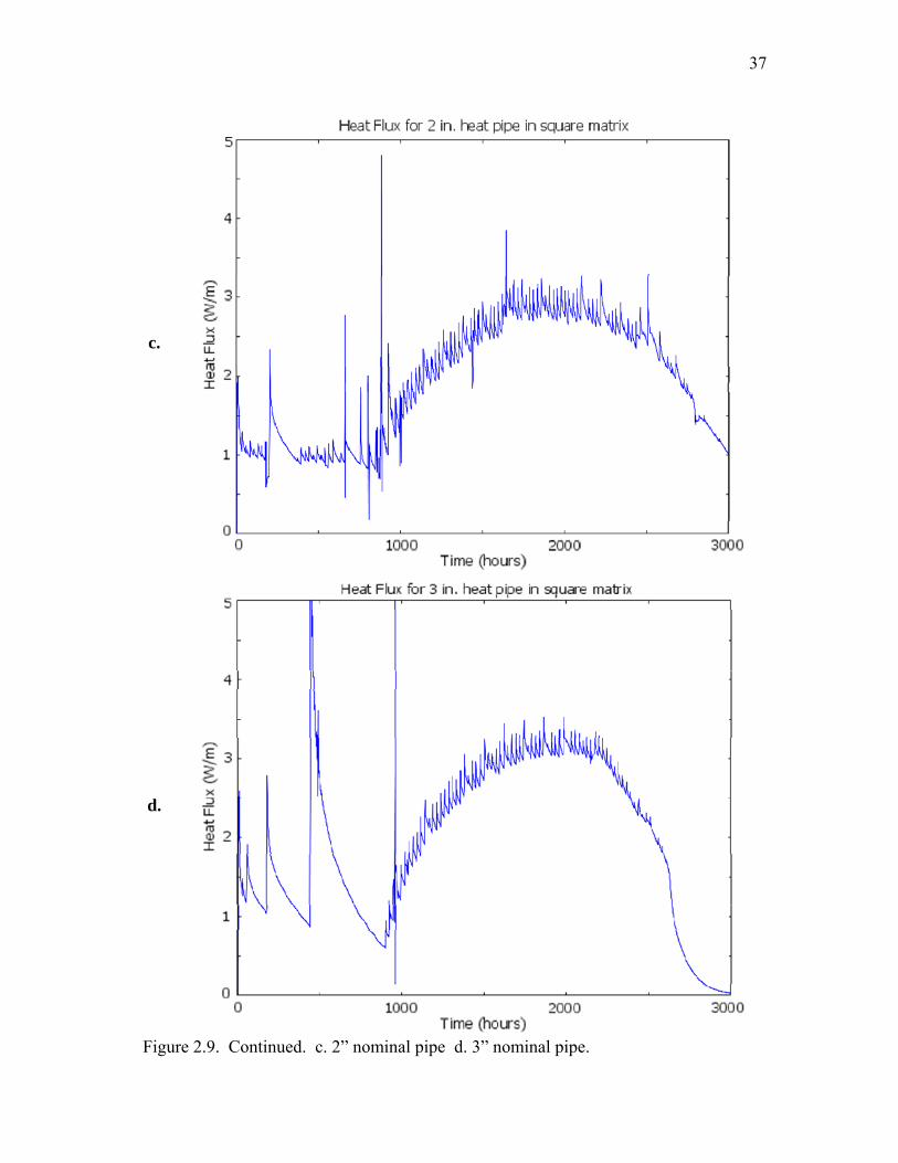
Figure 2.9 shows the heat flux throughout the season for the various pipe

diameters. The function for heat capacity, Eq. (2.5), resembles a delta function, and the

function for thermal conductivity, Eq. (2.2), is similar to a step function. Because of the

near discontinuities associated with these two functions at the freezing temperature, the

model becomes partially unstable. This instability is exhibited by the large peaks in heat

flux at the thermosiphon wall when freezing begins.

Discussion

A comparison of the results obtained in this simulation to results obtained for a

design of a ground loop heat exchanger done by Spitler in his software package

GLHEPro [6] shows that a common ground loop heat exchanger using common practice

technology requires 2.5 times the amount of drilling depth that a STA would require.

35

Table 2.1. Results of optimization study. Nominal Pipe

Diameter Outer Diameter Final Temperature at equilibrium

Total Heat Transferred per length

(mm) (in.) (°C) (°F) (kJ/m) (Btu/ft.) 1/2" 21.34 0.840 -0.06 31.9 125,340 36,210 1" 33.40 1.315 -0.12 31.8 144,778 41,826

1 1/2" 48.26 1.900 -1.45 29.4 154,604 44,664 2" 60.33 2.375 -3.42 25.8 158,003 45,646

2 1/2" 73.03 2.875 -3.58 25.6 156,669 45,261 3" 88.90 3.500 -4.80 23.4 156,902 45,328 4" 114.3 4.500 -5.06 22.9 152,098 43,940 5" 141.3 5.563 -5.37 22.3 145,525 42,041

The example that Spitler uses in GLHEPro has a total cooling load of 95,646 kW-

hr, as shown in his Table 1. GLHEPro indicates that for this load, 3,796.7 m (12,456 ft.)

of borehole would be required, corresponding to 25 kWh of load per meter (7.6 kWh/ft.)

of borehole drilling. In comparison, the results obtained from this simulation shows a

load of 62.4 kWh per meter (19.0 kWh/ft.) drilled, meaning the pipe and drilling cost of

this proposed heat pipe system will be approximately 40% that of a comparable ground

loop heating and cooling system.

There are a few reasons for this significant increase in performance.

Thermosiphons do not have heat transfer interference with a return line running adjacent

to a supply line (see Fig. 1.1) [7-9]. The thermosiphons modeled use metal tubing with

higher thermal conductivities than the plastics used in GLHEs. In addition, less power is

used by eliminating the compression refrigeration cycle, although the decrease in power

has no effect on pipe length or drilling depth.

As pipe diameter increases, the amount of heat transferred and the final

temperature of the domain reach asymptotic values that cannot be surpassed, limited by

winter temperature fluctuations. Because the total volume of ground between heat pipes

36

a.

b.

Figure 2.9. Half-year heat fluxes. a. ½” nominal pipe b. 1” nominal pipe.

37

c.

d.

Figure 2.9. Continued. c. 2” nominal pipe d. 3” nominal pipe.

38

e.

f.

Figure 2.9. Continued. e. 4” nominal pipe f. 5” nominal pipe.

39

goes down when the separation distance is fixed and the pipe diameter goes up, the total

heat capacity also goes down, and the total heat transferred drops away from the

asymptotic value. These effects indicate an optimum pipe diameter for a given

separation. It is assumed, therefore, that there is also an optimum separation for a fixed

pipe diameter. In practice, the pipe diameter is constrained by drilling techniques and by

the size of the equipment that is installed within the pipe. It is therefore more useful to

optimize pipe separation than pipe diameter.

Conclusions

For large-scale commercial design and optimization, COMSOL proves to be too

cumbersome, as shown by the difficulty to model actual conditions (artificial heat

transfer coefficients), too slow, with runtimes exceeding three days, lengthy post-

processing times, manual extraction of certain data, difficult to run batch jobs, and unable

to represent phase changes adequately (heat capacity and thermal conductivity equations

with discontinuities). Another model is necessary that is capable of accurately

representing phase changes. The numerical method used and the process of determining

time steps is unknown, which is another reason COMSOL was abandoned for original

code.

From preliminary simulations, thermosiphon UTES appears to be a viable energy

savings solution competitive with and comparable to GSHPs. Although an entire climate

control system using thermosiphons appears to have an initial installation cost similar to

GLHEs (thermosiphons have a lower cost for drilling and pipe, but an additional cost for

heat exchangers; see Appendix A), the operational cost promises to be much lower than

any widespread technology currently in use.

40

The design of thermosiphons installed in the ground can be optimized with

optimum design parameters being found through a straightforward set of simulations.

For 1-m (3.3 ft.) spacing, the optimum pipe was found to be a 2-inch nominal sch. 40

aluminum pipe.

References

[1] COMSOL Multiphysics Software version 3.3. [2] Austin, W., Yavuzturk, C., and Spitler, J.D., 2000, “Development Of An In-Situ System For Measuring Ground Thermal Properties,” ASHRAE Transactions, 106(1), pp. 365-379. [3] Cengel, Y., and Boles, M., 2008, Thermodynamics: An Engineering Approach, 6th ed. McGraw-Hill, pp. 909-957, Appendix 1. [4] University of Utah Department of Atmospheric Sciences, June 2007, “Download KSLC Data”. http://mesowest.utah.edu/cgi-bin/droman/download_ndb.cgi?stn=KSLC& hour1=18&min1=36&timetype=LOCAL&unit=0&graph=0 [5] Kumar, V., Gangacharyulu, D. and Tathgir, R. G., 2007, “Heat Transfer Studies of a Heat Pipe,” Heat Transfer Engineering, 28:11, pp. 954-965. [6] Spitler, J.D, 2000, “GLHEPRO—A Design Tool For Commercial Building Ground Loop Heat Exchangers,” Proceedings of the Fourth International Heat Pumps in Cold Climates Conference, Aylmer, Quebec. [7] Yavuzturk, C., Spitler, J.D., and Rees, S.J., 1999, “A Transient Two-dimensional Finite Volume Model for the Simulation of Vertical U-tube Ground Heat Exchangers,” ASHRAE Transactions. 105(2), pp. 465-474. [8] Yavuzturk, C., Spitler, J.D., 1999, “A Short Time Step Response Factor Model for Vertical Ground Loop Heat Exchangers,” ASHRAE Transactions. 105(2), pp. 475-485. [9] Muraya, N.K., O’Neal, D.L., and Heffington, W.M., 1996, “Thermal interference of adjacent legs in a vertical U-tube heat exchanger for a ground-coupled heat pump,” ASHRAE Transactions, 102(2), pp. 12–21.

CHAPTER 3

MODELING FREEZING AND MELTING

Explicit solutions are only available for a few simple phase change problems in

one dimension. Most phase change problems are not easily solved, or even

approximated, by the available explicit solutions. In order to “solve” a problem of this

nature, it must be simulated through some numerical method. Typically, such problems

have a large number of variables that are changing with time; therefore, a computer code

is favorable for keeping track of the large amounts of data. In order to calculate time-

dependent problems with a computer, the problem must be discretized. Variables that are

continuous functions of time or space, such as temperature and energy, must be replaced

with their values at discrete points, and at discrete time steps, small enough that the sense

of continuity is not lost. For a computer to solve a problem numerically, derivatives and

integrals must be replaced by finite-differences and sums.

Methods

The Enthalpy Method

Although there are other methods of numerically simulating phase change

problems such as front-tracking methods, the enthalpy method (as described in [1]) is

favored because it does not force the Stefan condition on the solution. Rather, the phase

change interface is a natural boundary condition dependent on the internal energy of the

42

discrete point, allowing multiple phase change boundaries and disappearing phases,

which is classically observed in heat storage applications where there are charging and

discharging cycles. There are shortcomings to the enthalpy method, especially when

modeling phenomena where there is instability in the phase change interface, such as

supercooling.

The enthalpy method is based on the law of conservation of energy. The simplest

way to apply the conservation law is through an integral heat balance over a control

volume as in Eq. (3.1).

=∆ − ∙∆ (3.1)

Here t is time, E is energy per unit volume, or = , where ρ is density and e is energy

per unit mass. The heat flux into the volume V across surface S is − ∙ . One of the

advantages of the integral heat balance is its validity over multiple phases, even with

discontinuities in energy or heat flux.

To complete the enthalpy method, the volume occupied by the phase change

material is divided into a finite amount of control volumes , with i ranging from 1 to N,

with N being the number of control volumes, and energy conservation, Eq. (3.1), is

applied to each. From the equation of state described in Eq. (B.1), with = 0

representing a solid substance at its melt temperature (Tm), if ≤ 0, is solid, if ≥ , is liquid, and if 0 < < , then is part solid and part liquid, or slushy,

where L is the latent heat of fusion. The liquid fraction in a slushy control volume is

defined as:

= (3.2)

43

Unlike the analytical solution of Appendix B, the exact location of the solid-liquid

interface is unknown and is not part of the enthalpy method calculation but can be

recovered afterward.

Enthalpy Method in Cylindrical Coordinates

Again, since the problem under consideration is simplest in cylindrical

coordinates, that is how the enthalpy method will be worked in detail, using a similar

setup to the analytical solution presented in Appendix B. Consider a hollow cylinder,

with inner radius / and outer radius / , as in Fig. 3.1, where N is the number of

nodes in the domain. The cylinder being made up of a phase change material that

changes phase at a melt temperature , initially solid with the initial condition

( , 0) = ( ) ≤ , / ≤ ≤ / (3.3)

where T is temperature and T(r,0) is the temperature, as a function of radius r, at the

initial time t=0.

Conservation of energy applied to one-dimensional radial control volumes of

height Δz

= / − / ∆ (3.4)

where i represents a particular node and ranges from 1 to N, turns into

2 ∆ ( , ) =− 2 ∆ ( , )

(3.5)

Here, q’’ is the heat flux, or the energy transfer rate per unit area, and n is the time step.

44

Figure 3.1. General model geometry with even node spacing to N nodes.

45

Integrating the derivatives in Eq. (3.5) leads to

2 ( , ) = 2 ′′ , − ′′ ,

(3.6)

If it is assumed the volumetric energy density ( , ) does not vary over ∆ , that is,

between / and / , and if the timestep is small enough that the heat flux can be

assumed constant over ∆ , the equation can be fully discretized, as a time-explicit

scheme,

[ ( , ) − ( , )]( − )= 2∆ ′′ , − ′′ ,

(3.7)

It can be shown that

− = 2 ∆ (3.8)

and therefore,

( , ) = ( , ) + ∆∆ ′′ , − ′′ , (3.9)

From the applicable heat equation and corresponding solution for temperature, it can be

shown using Fourier’s Law that the heat transfer between node i-1 and i is

= ( − ) (3.10)

46

Here, the notation is continued to show the discrete spatial nodes with a subscript, and a

superscript is introduced to indicate the discrete time-step. The resistance to heat transfer

is

= ln + ln (3.11)

Combining Eq. (3.9) and Eq. (3.10), with the discrete notation,

= + ∆∆ ( − ) + ( − ) (3.12)

Now, a new heat transfer term, q, that resembles a heat transfer rate per unit length, can

be introduced to simplify the equations,

= ( − ) (3.13)

Model Process

By discretizing the boundary conditions and initial values, there is enough

information to numerically model the problem of interest. Initially, temperatures of all

the nodes are known.

Initial values:

= ( ) ≤ , = 1,… , (3.14)

The thermal properties of the phase change material are considered constant within a

phase, therefore

47

= [ − ], <[ − ] + , >= (3.15)

where cS and cL are the specific heats of the solid and liquid phases, respectively. With

all the initial temperatures and internal energies (and subsequently, the phase) of every

node known, the problem can be solved with a time-explicit scheme by stepping forward

in time once it is decided how the thermal conductivities of slushy nodes are to be

determined.

Thermal Conductivity Models

If the phase boundary is moving sharply perpendicular to the direction of heat

transfer, the resistances of the two phases is additive, with the thickness of each phase

determined through the liquid fraction. Therefore, the thermal conductivity, k, can be

determined from

1 = ( ) + 1 −( ) (3.16)

Alternatively, if the phase change in slushy nodes is occurring in columns parallel to the

direction of heat transfer, the conductivities are additive, and the overall thermal

conductivity is

= ( ) + (1 − ) ( ) (3.17)

When the thermal conductivity is a function of temperature only, the Kirchoff

temperature, u, can be employed in place of T.

= [ − ], <[ − ], > 0, = (3.18)

If the equation for heat flux, Eq. (3.13), is reformulated in terms of u,

48

= −ln (3.19)

Therefore, using the Kirchoff temperature eliminates the need to calculate a thermal

conductivity value for slushy nodes, since they are treated as isothermal and do not

contribute to the heat transfer.

Once the boundary conditions are established, the energy density of each node

can be calculated for the next time step,

= + ∆∆ / − / , = 1,… , (3.20)

The temperatures at each node can be recalculated,

= + / , ≤ 0+ ( − )/ , ≥ 0 < < (3.21)

as well as the liquid fraction

= 0, ≤ 01, ≥/ , 0 < < (3.22)

At this point, the time-step can be advanced, and new conductivities, resistances,

and Kirchoff temperatures can be calculated. A complete numerical solution is obtained

through advancing time-steps until the desired time is covered.

Results

Code Validation

In order to model thermosiphons adequately, a computer code has to be developed

and checked for reliability. A computer code was written, included as Appendix C,

capable of modeling a constant temperature boundary condition, a constant flux boundary

49

condition, and the eventual transient ambient temperature boundary condition used to

model STAs. The code could easily be modified to accommodate other boundary

conditions as well, such as a convection or radiation boundary. The three methods of

determining thermal conductivity of slushy nodes, presented in the previous section, are

also represented by the model.

Temperature Boundary Condition

The first test for a heat transfer model of a hollow cylinder is to verify that it

matches the known solution for temperature boundary conditions at the inner and outer

radius. The known steady-state solution for the temperature profile within the wall of a

hollow cylinder is [2]

( ) = / − /ln / / ln / + / (3.23)

where T1/2 is the temperature at the inner surface, and correspondingly, TN+1/2 is the

temperature imposed on the outer surface. Additionally, r1/2 and rN+1/2 are the inner and

outer radius, respectively. Here, it can be seen that the units of temperature and radius

are irrelevant as long as they are consistent. In addition, the thermal properties of the

cylinder do not have any effect on the steady-state solution. As a test to the code, a

specific scenario is proposed for comparison. By setting / = 1℃ (33.8°F) and

/ = 25℃(77° ), with / = 0.0254m (1 in.) and / = 0.25m (9.84 in.), the

results for various r are shown in Table 3.1. For information on how to do this

calculation using the code, see Appendix C.

50

Long before the simulation time of one year is completed, the temperatures have

stabilized at their steady-state values. The time-step for this simulation is irrelevant since

it is a steady-state solution. The results for the steady-state temperatures at various

locations are shown alongside the exact solution, in Table 3.1. Thermal conductivities

calculated through the sharp front and columnar freezing formulations yield identical

steady-state temperature results. When the thermal conductivity throughout the material

is a constant (i.e. only one phase exists), the three methods of determining the thermal

conductivity and subsequent resistances are mathematically identical.

The exact solution for the heat transfer rate through the hollow cylinder is

= 2 ( / − / )ln // (3.24)

where l is the length of the cylinder, and thermal conductivity, k, is 0.00058 W/mK.

Because the heat transfer rate in the simulation code is per unit length and per radian, the

Table 3.1. Temperature boundary condition modeled.

Node Radius cm (in.)

Temperature (Exact solution)

°C (°F)

Temperature (Modeled)

°C (°F) r1/2 2.5400 (1.0000) 1 (33.8) 1 (33.8) 1 2.7442 (1.0804) 1.8115 (35.2607) 1.8115 (35.2607) 2 3.3567 (1.3215) 3.9261 (39.0670) 3.9261 (39.0670) 3 4.3776 (1.7235) 6.7131 (44.0836) 6.7131 (44.0836) 4 5.8069 (2.2862) 9.6785 (49.4213) 9.6785 (49.4213) 5 7.6445 (3.0096) 12.5642 (54.6156) 12.5642 (54.6156) 6 9.8905 (3.8939) 15.2676 (59.4817) 15.2676 (59.4817) 7 12.5449 (4.93894) 17.7628 (63.9730) 17.7628 (63.9730) 8 15.6076 (6.14472) 20.0554 (68.0997) 20.0554 (68.0997) 9 19.0787 (7.51130) 22.1631 (71.8936) 22.1631 (71.8936)

10 22.9582 (9.03866) 24.1058 (75.3904) 24.1058 (75.3904) rN+1/2 25.0000 (9.84252) 25 (77) 25 (77)

51

comparable rate is

( ) = 2 = / − /ln // (3.25)

For the scenario presented, the solution to Eq. (3.25) for this flux is -6.0873 W/m

(-6.3309 Btu/h/ft.). To the same number of significant figures, the MATLAB code has an

identical result.

Flux Boundary Condition with Freezing

With the initial temperature at the melt temperature (0°C), and the initial phase

being liquid (with a liquid fraction of 1), the heat transfer rate at the inner boundary

needed to freeze the domain, in time t, per length, per radian is calculated by

= ( / − / )2 (3.26)

If t is taken to be one day, or 86,400 seconds, and rN+1/2=0.5, r1/2=0.1, with L=360

kJ/kg, then qr is -0.5 kW/m. By setting a flux boundary condition at the inner radius to -

0.5 kW/m, the model should show an entirely frozen domain after one day (simulation

time). In reality, the first node will be at a temperature lower than the melt temperature

before the outer node is frozen, but the total energy necessary to freeze the domain will

have been removed. Therefore, as a method of verification, the total energy in each node

is calculated (e) and summed, Eq. (3.27), and the simulation is stopped when this sum is

below zero.

= = (( + 0.5Δ ) − ( − 0.5Δ ) ) (3.27)

52

With N=10, and any of the thermal conductivity modes employed, = 0 / at = 86,400.04s. The error is 0.00005%, most likely resulting from the propagation

of rounding errors, which is certainly small enough to accept the simulation code as

having an adequate mathematical formulation of the energy balance during a freezing

process.

Flux Boundary Condition With Moving Melt Front

The boundary conditions for the problem are

′′ / , = −2 / , > 0 (3.28)

′′ / , = 0, > 0. (3.29)

where Q is the line heat source (W/m) centered at r=0.

Note the necessary differences between the setup of the problem here and in

Appendix B. In order to simulate the problem numerically, values must be finite. The

two boundary conditions expressed by limits, Eq. (B.14) and Eq. (B.15), have to be

approximated by making / / / ≈ 0. The semi-infinite domain is simulated by not

allowing time to get significantly large. That is, the line- source heat flux should have

little effect on the material near the outer radius. The phase change interface should be

maintained closer to the inner radius to make valid comparisons with the analytical

results.

In order to solve the particular problem presented in Appendix B, the boundary

condition at r=r1/2 is set to

/ = (3.30)

Additionally, the boundary condition at r=rN+1/2 is

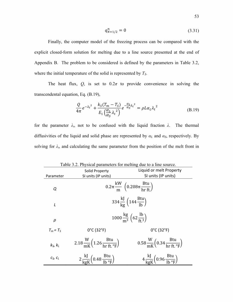
53

/ = 0 (3.31)

Finally, the computer model of the freezing process can be compared with the

explicit closed-form solution for melting due to a line source presented at the end of

Appendix B. The problem to be considered is defined by the parameters in Table 3.2,

where the initial temperature of the solid is represented by TS.

The heat flux, Q, is set to 0.2π to provide convenience in solving the

transcendental equation, Eq. (B.19),

4 + ( − ) = (B.19)

for the parameter λt, not to be confused with the liquid fraction λ. The thermal

diffusivities of the liquid and solid phase are represented by αL and αS, respectively. By

solving for λt, and calculating the same parameter from the position of the melt front in

Table 3.2. Physical parameters for melting due to a line source.

Parameter Solid Property

SI units (IP units)Liquid or melt Property

SI units (IP units)

Q 0.2π kWm 0.208π Btuhr ft.

L 334 kJkg 144Btulb

ρ 1000 kgm 62 lbft.

Tm = TS 0°C (32°F) 0°C (32°F)

kS, kL 2.18 WmK 1.26 Btuhr ft. °F 0.58 WmK 0.34 Btuhrft. °F

cS, cL 2 kJkgK 0.48 Btulb °F 4 kJkgK 0.96 Btulb°F

54

the simulation using Eq. (B.16)

( ) = 2 , > 0 (B.16)

the two can easily be compared. For this particular scenario, the transcendental equation

for λt , Eq. (B.19), gives = 0.7608.

With a flux boundary condition, / = 0.001 m (0.039 in.), / = 50m (164

ft..), and = 100, the location of the melt front (Rmelt) is determined by searching for the

node with a liquid fraction (λ) between 0 and 1, and for that node, calculating

= + ∆ ( − 0.5) (3.32)

Subsequently, λt can be calculated from Eq. (B.16). A graph of R(t) and λt for the model

compared with values calculated from the closed-form solution is shown in Fig. 3.2.

Under these conditions, λt, determined from the model, oscillates between 0.432

and 0.865 initially. As the model progresses, the oscillations are dampened. A running

average of λt steadies at a value of 0.768.

The overall melt rate calculated by the model matches the closed-form solution

well. However, as the melt front reaches the boundary of a node, the melting rate

increases, only to subsequently decrease after passing the boundary. Because the energy

is balanced, the overall melt rate is equivalent to the closed-form solution. The

instantaneous melt rate and the actual position of the melt front does not need to be

precise; therefore, the model is ready to be used with a transient temperature boundary

condition to optimize and design underground thermal energy storage systems using

smart thermosiphons. It should be noted that specific information about instantaneous

55

rates of melting and positions of phase change boundaries should be regarded as

imprecise values, but the overall energy of the model is balanced.

MATLAB Design Methodology

This section describes the incorporation of the freezing and melting model

developed in the previous section into a more complete, and adaptable, code to be used in

designing underground smart thermosiphon arrays. In order to be a viable methodology,

the program has to be capable of modeling transient seasonal weather effects, and it has

to be able to do it quickly.

Figure 3.2. Modeled melt radius R(t) and λt compared to closed-form solution.

0

0.1

0.2

0.3

0.4

0.5

0.6

0.7

0.8

0.9

1

0 100 200 300 400

Mel

t Rad

ius (

m) a

nd λ

t

Time (hours)

Modeled R Calculated R Modeled λt Calculated λt

56

Weather Data The previous sections described the calculations that are to be performed each

time-step in the model process, but the peripheral calculations and the setup of the

problems have not described. In order to size thermosiphon systems, a full year has to be

modeled with as many temperature transients modeled as possible. Published weather

information, specifically ambient outdoor air temperature, is typically reported for every

hour of the year [3], but can be found at smaller intervals [4]. It is considered that, for the

purposes of this analysis, 8,760 outdoor temperature readings per year are sufficient for

the design of a heating, ventilating, and air-conditioning (HVAC) system. The 8,760-

hour model is accepted as the standard for energy modeling practice [5], and therefore is

a common limitation of programs used to model building and HVAC energy.

Because the MATLAB design code has the capability of changing the boundary

temperature at any time interval chosen based on a database, the parametric empirical

formula for ambient temperature, used in Chapter 2 for the COMSOL modeling, is

unnecessary.

As a robust representation of yearly temperature fluctuations, a typical

meteorological year (TMY) file is selected as the ambient boundary conditions in the

model. The TMY files contain hourly meteorological values that represent conditions at

a particular location over a long period, such as 30 years [6].

Model Geometry

Smart thermosiphon arrays (STAs) imply a repeating arrangement of

thermosiphons. An irregular arrangement of thermosiphons could be reasonable in

practice as an attempt to minimize losses from edge thermosiphons or adjust for site-

57

specific features, such as a partially shaded area or varied soil compositions. These

situations are complicated, difficult to model, requiring 2-D or perhaps 3-D models, and

are usually particular to single jobs.

Multiple options are available for regularly repeating patterns of thermosiphons in

an STA. In Chapter 2, a hexagonal unit and a square array were presented. It is logical,

in avoiding irregular arrangements, to use repeating patterns of evenly spaced

thermosiphons. It is also deemed reasonable to assume, because the influence of any

single thermosiphon pipe is a cylinder, the tightest arrangement possible is optimal.

Therefore, the geometry chosen for all design optimizations is a hexagonal array of

thermosiphons, as is shown in Fig. 3.3.

To be entirely consistent with a hexagonal array, the model should be represented

Figure 3.3. Geometry of hexagonal array, showing area not modeled (Alost) by chosen method.

58

in a 2-D Cartesian coordinate. Based on the symmetry of the system, the 30-60-90

triangle shown to the upper right of the center thermosiphon would be the domain

modeled. The base of that triangle is half the distance of separation between

thermosiphons.

In an attempt to simplify, and therefore, speed up the modeling process, a 1-D

cylindrical system is favored over the 2-D model. By assuming the domain is contained

in the circle, with a radius of half the separation, shown in Fig. 3.3, the total area modeled

is decreased. In terms of the radius, the area not accounted for ( ) by going to

cylindrical geometry is

= 2√3 − (3.33)

The area modeled is 90.7% of the true area and should be accounted for in the design of

thermosiphon arrays, especially when considering the amount of thermal storage

available. In addition, a cylindrical model allows a more accurate representation of heat

transfer at the circular boundary formed by the thermosiphon pipe. This heat transfer is

considered more crucial to the design of a thermosiphon system than the heat storage lost

by going to a radial system.

The models presented in this manuscript do not account for Alost. The model can

be corrected by generating a different outer radius for the model that would yield an area

equal to the hexagon. This radius (rmodel) would be expressed, in terms of the separation

between thermosiphons, as

= 3 .√2 (3.34)

The radius of Eq. (3.35) is a 5% increase in the radius over what is used in the design

methodology.

59

Nodal Radii

The enthalpy formulation used to create the melting and freezing model is a finite

difference method, where the system being modeled is divided into individual segments

called nodes. In a one-dimensional radial system, the centers of these nodes have a

radius (ri), where i is the node number, and a radial dimension (∆ ). Constant∆ , or

evenly spaced nodes, is a typical selection for a finite-difference model. For simplicity,

evenly spaced nodes was the initial selection for the design methodology.

All thermal properties are assumed constant across a node, including the

temperature and energy. Therefore, the model becomes more accurate as the number of

nodes (N) becomes larger. However, every decrease in the minimum∆ , which comes

from an increase in the number of nodes, decreases the size of each time-step, to maintain

stability. With more time-steps to calculate, and more nodes to calculate, the

computational time increases significantly with each increase in N.

In order to minimize the length of time that it takes to model while still

maintaining an acceptable accuracy, evenly spaced nodes are not used. All of the heat

that is introduced to or removed from the domain modeled comes through the

thermosiphon wall, which is the inner radius, the boundary of the first node. Being the

smallest radius and the source of all heat, the area nearest the thermosiphon will have the

most variation in thermal properties and largest temperature gradients. Further from the

thermosiphon wall, the soil acts as a large thermal mass with little variation in properties.

Therefore, more nodes are needed near the thermosiphon than far away. Given

equivalent minimum node spacing, the time-steps for evenly spaced nodes and the time-

steps for nodes that increase in spacing with larger radius will be equivalent. However,

60

there is a reduction in computational time because there will be fewer nodes to calculate

with the uneven spacing.

There are many ways to determine the spacing of nodes. The method used in the

design methodology is based around the sum of consecutive numbers. If the domain is

split into N nodes, it can be further divided into 1+2+…+(N-1)+N equally spaced

segments (see Fig. 3.4). Each node takes i segments, where i is the node number starting

from the inner radius. That is, the size of the node is

Figure 3.4. Increased node spacing based on consecutive sums.

61

∆ = ∑ ( / − / ) (3.35)

Therefore, the radius of the node is

= / + 2 + ∑ ( − 1)∑ ( / − / ) (3.36)

Although there are other ways to size the nodes after the same fashion, this method is

used. Calculating nodes this way accomplishes the two goals of reducing the total

number of nodes and maintaining a small node near the inner radius. This pattern also

allows for a whole number of nodes, which is a necessary criterion for the selection of

node spacing.

The size of each time-step needs to be small enough to maintain stability. For the

purposes of the design methodology, the size of the time-step (∆ ), in seconds, is

conservatively determined by

∆ = min (∆ )2.1 , , 3600 (3.37)

where (∆ ) is the minimum node size, and , is the maximum thermal

diffusivity for either the liquid phase (L) or the solid phase (S). Equation (3.38) is based

on the Courant-Friedrichs-Lewy (CFL) condition [7]

∆ ≤ ∆2 (3.38)

The boundary conditions change every hour; therefore, the time-step cannot exceed 3600

seconds.

62

References

[1] Alexiades, V., and Solomon, A.D., 1993, Mathematical Modeling of Melting and Freezing Processes, Hemisphere Publishing Corporation. p. 211. [2] Incropera, F.P. and Dewitt, D.P., 2002, Fundamentals of Heat and Mass Transfer, John Wiley & Sons, New York NY, 5th Edition, p. 106. [3] National Renewable Energy Laboratory, 2009, “National Solar Radiation Data Base, 1991-2005 Update: Typical Meteorological Year 3”. http://rredc.nrel.gov/solar/old_data/ nsrdb/1991-2005/tmy3/ [4] University of Utah Department of Atmospheric Sciences, June 2007, “Download KSLC Data,” http://mesowest.utah.edu/cgi-bin/droman/download_ndb.cgi?stn=KSLC& hour1=18&min1=36&timetype=LOCAL&unit=0&graph=0 [5] ASHRAE, 2007, ANSI/ASHRAE/IESNA Standard 90.1-2007, Energy Standard for Buildings Except Low-Rise Residential Buildings, American Society of Heating, Refrigerating and Air-Conditioning Engineers, Inc., Atlanta, GA, Appendix G. [6] Wilcox, S., and Marion, W., 2008, “Users Manual for TMY3 Data Sets”. Technical Report NREL/TP-581-43156. [7] Courant, R., Friedrichs, K., and Lewy, H.,1928, “Uber die partiellen differenzen-gleichungen der mathematischen Physik,” Mathematische Annalen, 100, pp. 32-74.

CHAPTER 4

PILOT SCALE

This chapter details the design, installation, and operation of a pilot scale

implementation of a smart thermosiphon array (STA) on a residential property in

Midvale, Utah. The design is based on the results from the computer modeling and

preliminary optimization performed in COMSOL.

Methods

The thermosiphon pipes were constructed using seven galvanized steel pipes with

a 2 in. nominal pipe diameter and 3 m (10 ft.) in length. In order to seal the bottom of the

pipes, circles cut from a galvanized steel plate were welded on to one end. Neither

threaded caps nor standard weld-on caps could be used because they would have

exceeded the inner diameter of the drill sheath using direct-push drilling. The top,

uncapped end of the pipe was threaded.

Three of the seven pipes were instrumented with 10 thermocouples each, evenly

spaced at 30 cm (1 ft.) increments, placed on the outside of the pipes. Attached to the

other four pipes were five thermocouples each, evenly spaced at 61 cm (2 ft.) increments.

Seven boreholes 3 m (10 ft.) deep, located 1.5 m (5 ft.) apart, with six forming a

hexagon around one in the center (Fig. 4.1), were drilled using a direct-push method of

drilling (Fig. 4.2). Instead of using a rotary drill bit, direct-push utilizes an expendable

64

tip that is left at the bottom of each hole. The drill rotates minimally and has a percussion

hammer to penetrate denser and harder soils. Based on commercial bids, GeoProbe

installation costs are about one-tenth the cost of drilling a 20 cm (8 in.) borehole using

conventional methods. Direct push installation also eliminated the need for drilling mud

and handling removed soils. This drilling and the pipe locations are shown in Fig. 4.2 to

Fig. 4.4. The pipes were installed and temporarily capped to prevent contamination.

In addition to the seven boreholes for the thermosiphon pipes, three 4.3 m (14 ft.)

deep temperature monitoring wells were drilled. One monitoring well was located 15 cm

(6 in.) from the center thermosiphon, another well was located in the center of the three

thermosiphons with 10 thermocouples, and the third well was located 1.5 m (5 ft.) outside

the hexagon array.

The inside of the thermosiphon pipes were lined with fiberglass window screen

and held tight against the surface by shaped welded wire mesh. The DIN 43650a

Figure 4.1. Arrangement of seven thermosiphon pipes for pilot scale. Thermosiphons are indicated by a “T”, temperature monitoring wells indicated by W1,W2, and W3.

65

Figure 4.2. Direct-push drilling, using a pneumatic hammer and expendable tip.

Figure 4.3. Thermosiphon pipes installed. Pipe locations indicated with red arrows.

66

electrical connectors on Gotec ELS-50 30W electromagnetic pumps were removed so the

pumps could fit inside the pipes and could have sealed electrical connections. Hose

strainers were attached to the bottom of the pumps in order to prevent failure from debris.

Wired in series with the pumps, and located 15 cm (6 in.) above the pump inlets, were

stainless steel metal float switches (Fig. 4.5), supplied by APG Sensors, model LFS-V-

5G. The float switches were attached in shaped metal plates that held the tube, the

switch, and the wires, so the float could move unimpeded inside the thermosiphon pipes.

Individual 1.5 m (5 ft.) square flat panel heat exchangers were constructed for

each thermosiphon. Each copper heat exchanger consisted of 40 vertical 1.5 m (5 ft.)

tubes, 15.9 mm (0.5 in. nominal) diameter, connected by headers.

Figure 4.4. Thermosiphons with heat exchangers.

67

In order to connect the heat exchanger, the annular tube, the thermosiphon pipe,

and the wires from the pump and float switch, a special copper fitting was custom built,

shown in Fig. 4.6.

Two valves at the top of the thermosiphon are the vapor return line, 2.2 cm (0.75

in.) standard copper tubing , and the liquid supply line, 0.95 cm (0.25 in.) standard copper

tubing, that service the air conditioning load through the evaporator coil.

The system was tested for leaks with positive pressure and under vacuum. R-

134a was used as the working fluid. The array was charged in February 2010 and

experienced almost 2 months of freezing temperatures operating in a passive mode.

Data were gathered through a LabJack U6, a USB based measurement and

automation device which provides analog inputs/outputs and digital inputs/outputs, using

an experimental breadboard and multiplexer chips to accommodate 112 inputs. The

LabJack was controlled through MATLAB, using LabJack functions, connected to a

Figure 4.5. Float switch and pump assembly.

68

computer via USB. The LabJack also has the functionality to control the pump operation

during heat injection mode.

Data from temperature monitoring wells 15 days after the system was charged are

shown in Fig. 4.7. Only the quadrant of the array with the monitoring wells is shown,

symmetry can only be assumed for the other quadrants. The general temperature profile

is similar to the first month temperature profile from the calculations shown in Fig. 2.8.

A quantitative comparison is not practical since the model uses a different soil type and

saturation than the pilot scale. Unfortunately, the data acquisition system was irreparably

Figure 4.6. Pipe connectivity at top of thermosiphon pipe.

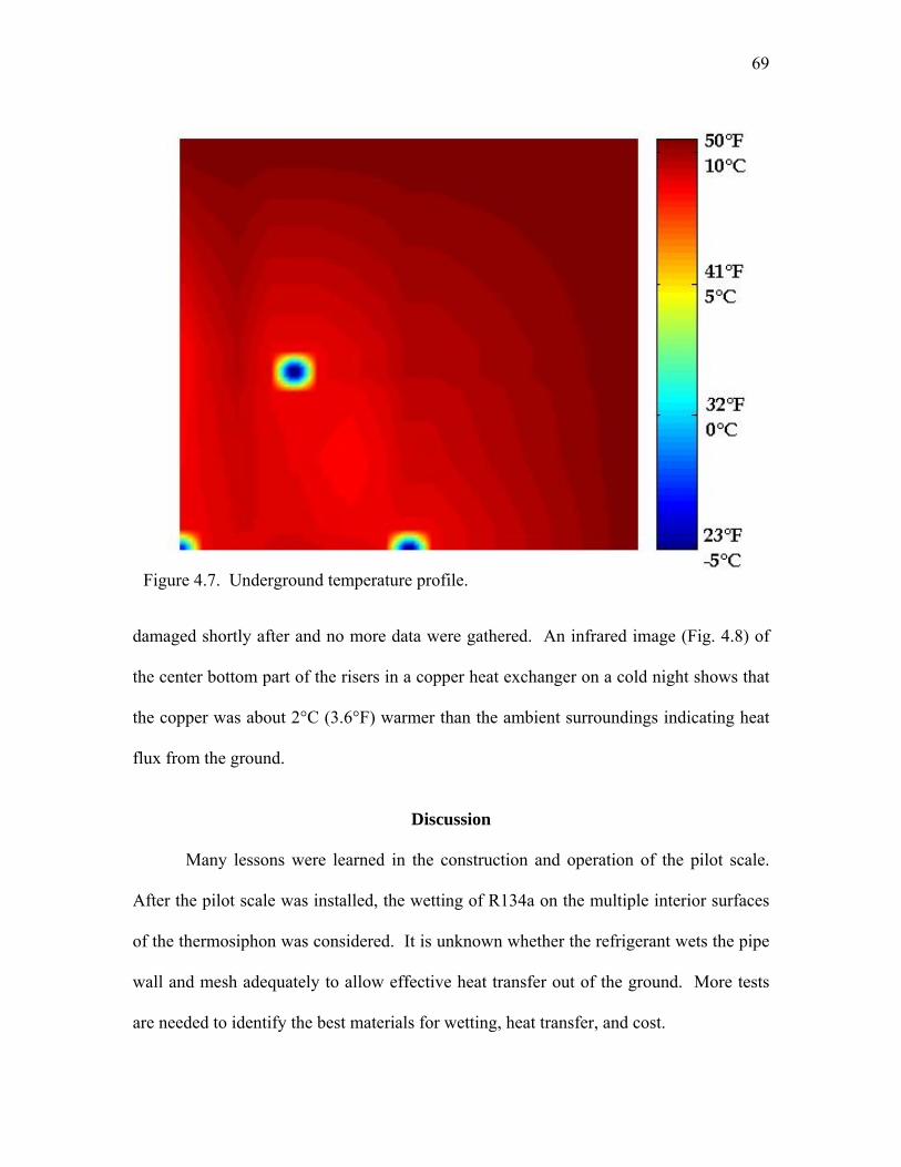
69

damaged shortly after and no more data were gathered. An infrared image (Fig. 4.8) of

the center bottom part of the risers in a copper heat exchanger on a cold night shows that

the copper was about 2°C (3.6°F) warmer than the ambient surroundings indicating heat

flux from the ground.

Discussion

Many lessons were learned in the construction and operation of the pilot scale.

After the pilot scale was installed, the wetting of R134a on the multiple interior surfaces

of the thermosiphon was considered. It is unknown whether the refrigerant wets the pipe

wall and mesh adequately to allow effective heat transfer out of the ground. More tests

are needed to identify the best materials for wetting, heat transfer, and cost.

Figure 4.7. Underground temperature profile.

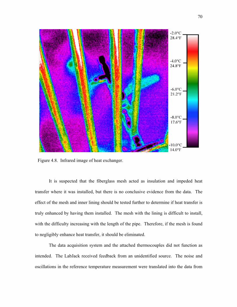
70

It is suspected that the fiberglass mesh acted as insulation and impeded heat

transfer where it was installed, but there is no conclusive evidence from the data. The

effect of the mesh and inner lining should be tested further to determine if heat transfer is

truly enhanced by having them installed. The mesh with the lining is difficult to install,

with the difficulty increasing with the length of the pipe. Therefore, if the mesh is found

to negligibly enhance heat transfer, it should be eliminated.

The data acquisition system and the attached thermocouples did not function as

intended. The LabJack received feedback from an unidentified source. The noise and

oscillations in the reference temperature measurement were translated into the data from

Figure 4.8. Infrared image of heat exchanger.

71

all of the thermocouples. It was also discovered that the range and precision of

measurement required is smaller than the tolerances and the reported error on most types

of thermocouples. Deformation in the thermocouple wire, among other things, could

cause enough noise and inconsistencies between thermocouples that the relatively small

temperature differences in the system would not be noticed. Resistance based

temperature measurements are recommended to achieve more precise results.

Even with the efforts to prevent contamination, debris made its way into the

thermosiphon pipes. This problem was resolved by removing the material with a vacuum

cleaner, but with the pipes installed in the ground, it was difficult to confirm that all

contaminants were removed. Standard threaded caps could not be used during

installation because they would not have fit inside the drilling sheath. Better caps should

have been devised for use.

After removing the electrical connections on the pumps, the wires were connected

with difficulty, and then were covered with liquid electrical tape. It was discovered later

that the tape did not adhere to the plastic of the pump and resulted in an electrical short.

A better design would include liquid tight electrical connections manufactured into the

pump. It should be remembered that the pump used was not designed for submersion.

The float switches were wired directly in series with the pumps. The series

wiring was done to reduce the number of wires that had to exit the pressurized pipe

through the wire feed-through fitting. For better control and data measurement, the float

switch signal should come to the surface independent of the power lines to the pump.

Control of the pump could then be more easily performed by a programmed control loop.

72

By wiring in series, the amperage limit of the float switch could be exceeded by the

pump’s electrical demand, requiring the float switch to be replaced.

Although the system was pressure tested at both positive and negative pressures,

five out of seven thermosiphon pipes would not hold their charge. Specific leak locations

could not be identified. The flat panel heat exchangers had 210 soldered joints each. The

pipes had two or three threaded joints (depending on the pipe) and one welded joint on

galvanized steel. Brazed fittings are the recommended joint type for R134a systems. The

heat exchangers should have been brazed together instead of soldered.

The heat exchangers were not structurally supported to withstand a high wind

load. One of the thermosiphons lost all of its refrigerant charge after being felled by a

wind storm. The connection between the thermosiphon pipe and the heat exchanger had

to be repaired. The movement on the fittings caused by the wind could possibly have

caused them to leak during windstorms even though they did not leak during pressure

tests.

After encountering enough problems, the pilot scale system was decommissioned.

There was no experimental control to the design, and the short period the system was in

operation was used as a brief demonstration of ground freezing using a thermosiphon

array.

Soil Analysis

There are several methods [1-3] of estimating soil thermal properties from their

composition. As seen previously, the thermal conductivity and heat capacity of the soil

is needed to model the heat transfer from the thermosiphon within the soil. These soil

properties can be measured in situ [4-7], which is the preferred method, especially in

73

regions where soil types vary drastically within the site. If an in situ method cannot be

used, a soil sample should be taken, and the thermal properties can be measured in a lab.

Lab measurements often lead to inaccurate results, however, due to changes in density

and water content with handling. As a less expensive alternative, or to confirm in situ

testing or laboratory testing, it is possible to use one of various empirical methods to

estimate the heat capacity and thermal conductivity.

Heat Capacity Approximations

The volumetric heat capacity of a mixture can be expressed as a weighted sum (or

average) of the heat capacities of the individual constituents.

= (4.1)

The volumetric heat capacity of each component is represented by , and represents

the volume fraction of n constituents. The volumetric heat capacity of each component is

equal to the specific heat of the component multiplied by the density.

= (4.2)

Here, the specific heat is represented by ci, and ρi is the density. Generally, it is easier to

use mass fractions (w), based on a dry mass, than volume fractions. The volume fractions

can be converted to mass fractions by multiplying the volume fraction by the component

density ratio:

= (4.3)

Here, ρb is the soil bulk density on a dry-mass basis. Substitution of Eq. (4.2) and Eq.

(4.3) into Eq. (4.1) produces

74

= (4.4)

In the de Vries approximation [3], it is assumed that dry soil can be broken into two

constituents, soil minerals and soil organic matter. Equation (4.4) can be rewritten as

= ( + + ) (4.5)

In this equation, uw is the gravimetric water content, defined as mw/mb, where mw is the

mass of the water, and mb is the dry mass of the bulk soil. The specific heats, cm, co, and

cw, are those of soil minerals, soil organic matter, and water, respectively. De Vries

reported in [3] the density, and specific heat, of common soil constituents at 20°C (68°F)

and atmospheric (sea level) pressure. These are shown in Table 4.1.

If the temperature varies greatly from 20°C (68°F), these values may require

adjustments.

Thermal Conductivity Approximations

Just as heat capacity can be approximated by knowing soil composition, empirical

formulas have been developed to estimate the thermal conductivities of the soil in a

similar manner [1-2, 8]. Unlike heat capacity, however, the thermal conductivity is not a

simple average of the individual components. The overall thermal conductivity depends

Table 4.1. Density and specific heat of various soil components.

Soil component Density Specific heat kg/m3 lb/ft3 kJ/kgK Btu/lb°F

Minerals (average) 2,650 165 0.73 0.29 Organic matter (average) 1,300 81 1.9 0.45

Water 1,000 62 4.18 1.00 Ice 920 57 2.0 0.48 Air 1.2 0.075 1.0 0.24

75

on the shape, composition, and configuration of individual components. It also is a

function of the porosity, water content, bulk density, and temperature.

Campbell [9] developed a relatively simple empirical formula to predict the

thermal conductivity (W/mK) of repacked soils that were measured in the laboratory by

McInnes [10].

= + 2.8 + (0.03 + 0.7 − )exp [−( ) ] (4.6)

where θv is the volumetric water content, and is the volume fraction of mineral solids,

which is the sum of the volume fraction of quartz, , and the volume fraction of

minerals other than quartz, . A and B are given by the equations

= 0.57 + 1.73 + 0.931 − 0.74 − 0.49 − 2.8 (1 − ) (4.7)

= 1 + 2.6. (4.8)

The density and specific heat of the minerals not quartz are normally taken to be the same

as clay. The mass fraction of clay is represented by mc.

If the soil is dry, = 0, and = 0.03 + 0.7 . The two extremes for thermal

conductivity in dry soil, therefore, are for = 0, which is no soil, and = 1,

representing pure solid material with no air, or water. In the first case, = 0.03W/mK

(0.017 Btu/hr/ft./°F), which is approximately the thermal conductivity of air. In the

second case, = 0.73W/mK (0.42 Btu/hr/ft./°F), which should be the thermal

conductivity of nonporous rock. Solid rock is reported to have a thermal conductivity

between 2 and 7W/mK (1.2 to 4 Btu/hr/ft./°F). While the empirical equation developed

by Campbell is not intended to predict the thermal conductivity of rock or anything but

soil, care must be taken in applying the formula to situations with high solids content,

76

with the understanding that the thermal conductivity will most likely be underpredicted if

the rock is assumed to be dry. Better predictions are obtained for nonporous rock when

simplifications are made based on the assumption of saturated soil with a low clay mass

fraction.

In the case where the soil is saturated, or when clay mass fraction is near zero, the

exponential term becomes zero, and = + 2.8 . This simplification has to happen

first, otherwise errors are introduced in the exponential term with a low clay mass

fraction. The absence of solids constitutes a limiting condition, = = = 0 , or

for pure water, = 0.57W/mK (0.33 Btu/hr/ft./°F). Another limiting condition is when = 1. In this case,

= 0.57 + 1.73 + 0.93(1 − )1 − 0.74 − 0.49(1 − ) (4.9)

which ranges from 2.94 to 8.85 W/mK (1.70 to 5.11 Btu/hr/ft./°F), for = 0, and = 1, respectively. These are better predictions for the thermal conductivity of solid

rock, with 8.8 W/mK (5.08 Btu/hr/ft./°F) being the reported thermal conductivity for

quartz [8].

The thermal conductivity predicted by this equation includes both the sensible

transfer of heat and the latent heat transfer. Because the latent heat transfer depends

greatly on temperature, adjustments should be made for varying temperature. The

thermal conductivities of water, 0.57 in Eq. (4.7), and air, 0.03 in Eq. (4.6), can be

adjusted for temperature to predict better overall conductivities from Eq. (4.6).

Lacking in the empirical equations of Campbell is the ability to predict the

thermal conductivity of frozen soils. Simpler equations that come from Kersten, [1],

77

predict the conductivity of frozen soils and unfrozen soils, for silt and clay soils, and for

sandy soils. The four equations for these conditions are:

1. Unfrozen silt and clay soils (at 4°C)

= [0.13 log( ) + 0.231] ∗ 10 . (4.10)

2. Unfrozen sandy soils (at 4°C)

= [0.1 log( ) + 0.258] ∗ 10 . (4.11)

3. Frozen silt and clay soils (at -4°C)

= 0.0014(10) . + 1.2 (10) . (4.12)

4. Frozen sandy soils (at -4°C)

= 0.011(10) . + 0.46 (10) . (4.13)

with the bulk density, , in units of grams per cubic centimeter, and is the

gravimetric water content. Unlike the equations developed by Campbell, Kersten’s

equations do not function at extrema. For example, Eq. (4.10) gives negative values for

conductivity when the gravimetric water content is below 1.7%, and Kersten advises not

to use this equation when the gravimetric water content is below 7%. Clay and silt retain

water well, however, and often have gravimetric water contents above that threshold.

Pilot Scale Soil

A core sample was taken with the Geoprobe drill out of one of the boreholes

when the pilot scale was installed. Over the 3 m (10 ft.) of depth, there was a great

variation in soil types. The top 0.6 m (2 ft.) consisted primarily of topsoil with the

surface being highest in organic materials. Between a depth of 0.9 m (3 ft.) and a depth

of 1.5 m (5 ft.) the soil consisted mostly of sand. Below 1.5 m (5 ft.) deep and down to

2.4 m (8 ft.) deep was a layer of clay. Below 2.4 m (8 ft.), there was almost nothing but

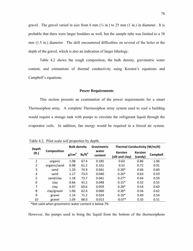
78

gravel. The gravel varied in size from 6 mm (¼ in.) to 25 mm (1 in.) in diameter. It is

probable that there were larger boulders as well, but the sample tube was limited to a 38

mm (1.5 in.) diameter. The drill encountered difficulties on several of the holes at the

depth of the gravel, which is also an indication of larger lithology.

Table 4.2 shows the rough composition, the bulk density, gravimetric water

content, and estimations of thermal conductivity using Kersten’s equations and

Campbell’s equations.

Power Requirements

This section presents an examination of the power requirements for a smart

Thermosiphon array. A complete Thermosiphon array system used to cool a building

would require a storage tank with pumps to circulate the refrigerant liquid through the

evaporator coils. In addition, fan energy would be required in a forced air system.

However, the pumps used to bring the liquid from the bottom of the thermosiphons

Table 4.2. Pilot scale soil properties by depth.

Depth (ft.) Composition

Bulk density Gravimetric water

content

Thermal Conductivity (W/m/K)

g/cm3 lb/ft3 Kersten (silt and clay)

Kersten (sandy) Campbell

1 organic 1.08 67.4 0.185 0.63 0.86 1.062 organic/sand 0.98 61.2 0.161 0.52 0.72 0.913 sand 1.20 74.9 0.041 0.28* 0.66 0.604 sand 1.17 73.0 0.040 0.26* 0.63 0.595 sand/clay 1.18 73.7 0.041 0.27* 0.64 0.596 clay 0.66 41.2 0.048 0.15* 0.32 0.557 clay 0.97 60.6 0.059 0.28* 0.54 0.608 clay/gravel 1.00 62.4 0.060 0.30* 0.56 0.629 gravel 1.14 71.2 0.024 0.10* 0.49 0.54

10 gravel 1.09 68.0 0.013 -0.07* 0.33 0.51*Not valid when gravimetric water content is below 7%

79

require little energy. The power required from the pump to supply the liquid to the

evaporator coil would be

= ∆ℎℎ (4.14)

where q is the cooling load, or the rate that energy is dumped into the heat sink of the

ground, ∆h is the head to be overcome by pumping, g is the gravitational constant, and is

hfg is the enthalpy of vaporization for the refrigerant. If R-134a is used as the refrigerant

at 0°C (32°F) for a 4.29 kW cooling load, and the pumps at the bottom of the

thermosiphons are 12 m (39 ft.) below grade, 2.54 W of pumping power would be

required, neglecting head loss due to friction and pump inefficiencies. The coefficient of

performance (COP) would then be 1690. A small solar photovoltaic panel could provide

this power requirement, producing a net-zero air conditioning system.

References

[1] Kersten, M.S., 1949, Thermal Properties of Soils, University of Minnesota, Eng. Exp. Station Bull, 28.

[2] Campbell, G.S., Jungbauer, J.D., Bidlake, W.R., and Hungerford, R.D., 1994, “Predicting the Effect of Temperature on Soil Thermal Conductivity,” Soil Sci. 158, pp. 307-313. [3] de Vries, D.A., 1963, “Thermal Properties of Soils,” Physics of plant environment, W.R. Van Wijk (ed.), North-Holland Publishing Company, Amsterdam, the Netherlands. pp. 210-235. [4] Austin, W., Yavuzturk, C., Spitler, J.D., 2000, “Development Of An In-Situ System For Measuring Ground Thermal Properties,” ASHRAE Transactions, 106(1), pp. 365-379. [5] Spitler, J.D., Rees,S.J., Yavuzturk,C., 1999, “More Comments on In-situ Borehole Thermal Conductivity Testing,” The Source, 12(2), pp. 4-6.

80

[6] Witte, H.J.L., van Gelder,G.J., and Spitler,J.D., 2002, “In Situ Measurement of Ground Thermal Conductivity: The Dutch Perspective,” ASHRAE Transactions. 108(1), pp. 263-272. [7] Spitler, J.D., Yavuzturk,C., and Rees,S.J., 2000, “In Situ Measurement of Ground Thermal Properties,” Proceedings of Terrastock 2000, Stuttgart, 1, pp. 165-170. [8] Bristow, K.L, 2002, “Thermal Conductivity”, Methods of Soil Analysis. Part 4. Physical Methods. J.H. Dane and G.C. Topp (eds.), Soil Science Society of America Book Series #5, Madison, Wisconsin. pp. 1209-1226. [9] Campbell, G.S., 1985, Soil Physics with BASIC. Elsevier, New York, NY. [10] McInnes, K.J., 1981, “Thermal Conductivities of soils from dryland wheat regions of eastern Washington,” M.S. thesis, Washington State University, Pullman, WA.

CHAPTER 5

DESIGN OPTIMIZATION RESULTS

In Chapter 3, the design and optimization methodology developed in MATLAB

was presented. This chapter presents results from various locations in the United States,

with various soil properties, for three different buildings.

Methods

Ambient Temperature Boundary Condition In Chapter 3, several boundary conditions were presented. In order to model the

thermosiphon array, a variation to those boundary conditions must be introduced.

Because of the symmetry of the problem (refer to Fig. 3.3), the outer radius of the domain

modeled is set as a zero flux boundary.

A TMY file is read into the simulation code. As the time-step advances, the

simulation time is calculated, and the inner boundary condition is taken to be the dry-bulb

outdoor air temperature from the TMY at that hour. However, due to thermosiphons

being gravity-assisted, they only operate in one direction; therefore, the outdoor air dry-

bulb temperature is only set as the boundary condition when the temperature in the first

node is larger. This condition limits the system to one-way heat transfer from the ground

to the outside air.

82

During hours when a cooling load exists that cannot be economized using outside

air, heat is transferred through the thermosiphon wall into the soil. If the ambient

temperature is greater than the temperature in the first node, and there is a load, a return

air temperature, , is calculated based on the load according to Eq. (5.1)

= / + (5.1)

The maximum return temperature would be a few degrees more than the thermostat

setting. Therefore, if the calculated return temperature is larger than the thermostat

setting, the return temperature is set equal to the thermostat setting, and the time-step is

counted as unmet cooling time. After the simulation is finished, the unmet cooling hours

are totaled. Whether the return temperature is calculated per Eq. (5.1) or is equal to the

thermostat setting, it is set as the inner boundary condition.

Because the return temperature should not greatly exceed the thermostat setting,

the temperature in the first node is also never larger than the thermostat setting. So, if

there is a load and the ambient outdoor temperature is lower than the first node

temperature, the load is considered to be economized and is not transferred to the ground

through the thermosiphon.

If there is no load, and the outdoor ambient temperature is greater than the first

node temperature, the thermosiphon wall becomes a zero flux boundary condition.

Design Optimization

In order to design a system of smart Thermosiphon arrays, a certain number of

parameters need to be constrained. The thermal properties of the soil should be measured

or calculated. The hourly load to be satisfied needs to be calculated for 8760 hours, and

83

hourly outdoor temperature for the location, spanning the same time, are needed. The

radius of the borehole where the thermosiphon is to be installed is affixed a value. The

initial temperature of the domain to be modeled is determined as the average temperature

over the course of the year.

The sphere is the optimal geometry for energy storage because it has the smallest

surface area to volume ratio. It is not practical to form a sphere of frozen soil under the

ground through the smart thermosiphon array (STA); therefore, a cylinder with the

diameter equal to its height is set as the geometrical constraint. With this constraint, the

total length of thermosiphon pipe and the distance of separation between thermosiphons

can be calculated from the number of thermosiphons and the total volume of the system.

The design is considered optimized when the length of thermosiphon pipe is

minimized, with the load being satisfied. The warm-season temperature conditions

reported by the American Society of Heating, Refrigeration, and Air conditioning

Engineers (ASHRAE) are based on annual percentiles of 0.4, 1.0, and 2.0 [1]. It is

standard practice for designing HVAC systems to size the system based on one of these

percentiles. If the smart thermosiphon array is designed around the one percentile

temperature condition, 1% of the year the ambient outdoor air temperature will exceed

the design temperature, and the system will be unable to meet the load. Therefore, the

load is considered satisfied when the load is unmet less than 87.6 hours.

The internal energy for a sample of soil decreases with temperature. If it is

assumed the minimum temperature of the soil is the minimum outdoor air temperature,

the minimum achievable energy of the soil can be determined with Eq. (3.15). In the

same way, the maximum temperature leads to the maximum energy. The difference

84

between the maximum and the minimum energies is the largest amount of energy that can

potentially be stored in the soil. The integrated, or total, load for the entire year divided

by the difference in the maximum and minimum energy yields the smallest volume of

soil that could possibly satisfy the cooling load. Using this volume as a starting point,

with a specified number of thermosiphon pipes, the volume can be increased and the

simulation run until the unmet load time is below 87.6 hours.

The number of thermosiphon pipes in an array is constrained to the series:

= 1 + 6 ( = 1,2,3,… ,∞) (5.2)

This constraint is based on a hexagonal array composed of N concentric hexagons with

one in the center. Starting with seven thermosiphon pipes, the volume is found that

yields less than 87.6 unmet load hours, the number of concentric hexagons is increased

by one, and the optimal volume for this array is found. This process is continued until

the length of pipe in the minimum volume for N+1, is larger than the optimal length of

pipe just found for N hexagons.

Building Load Calculations

The hourly air conditioning load for the three buildings was calculated by Trane

Trace 700 v6.2.6.5. Trane Trace 700 is accepted by American Society of Heating,

Refrigeration, and Air-Conditioning Engineers (ASHRAE) Standard 90.1-Appendix G

and the United States Green Building Council (USGBC) as approved energy modeling

software to show compliance with the Energy and Atmosphere prerequisite 2 (EAp2) as

part of the Leadership in Energy and Environmental Design (LEED) certification [2,3].

It is also accepted software for the energy modeling required by the Environmental

85

Protection Act (EPACT) under IRS Notice 2006-52, as amplified by IRS Notice 2008-40,

Section 4.

The three buildings included a residential house of 112 m2 (1200 sq. ft.), a mixed-

use facility with offices, classrooms, and retail, of 870 m2 (9400 sq. ft.), and a large office

building of 16,000 m2 (177,000 sq. ft.). The construction of each building was changed

to code minimum requirements for the location where it was modeled as required by

ASHRAE Standard 90.1 [4]. The U-factors (thermal transmittances) used for building

envelope construction and the SHGCs for glazing are shown in Tables 5.1 (SI units) and

5.2 (IP units).

ASHRAE has divided the United States into eight climate zones for establishing

code minimum requirements concerning the construction of the building envelope.

Within those eight climate zones, there are three sub classifications, A-moist, B-dry, and

C-marine. The eight climate zones are based on yearly temperatures [5]. Sixteen cities

were selected as locations for the three buildings modeled. These are shown in Tables

5.3 (SI units) and 5.4 (IP units) with their corresponding climate zone designation and

climatic data. The cities were selected based on the availability of TMY weather data

and highest population density within the climate zone. The weather monitoring station

numbers (WMO#) are listed in Table 5.3 for reference.

The heating dry bulb (DB) at a 99.6% design condition is a statistical temperature

used for design of heating systems. Statistically, 99.6% of all temperatures during any

given year should be above this temperature. The temperature only drops below the

heating DB design condition 0.4% of the year, or 35 hours. Likewise, the cooling DB is

86

Table 5.1. ASHRAE 90.1-2007 envelope requirements (U-values in W/m2/K)

Climate Zone 1A2

(A,B)3

(A,B,C)4

(A,B,C)5

(A,B)6

(A,B) 7

(A,B) 8

90.1-07 Residential Envelope

Requirements (wood-framed

w/ attic)

Roof U 0.15 0.15 0.15 0.15 0.15 0.15 0.15 0.12Walls U 0.51 0.51 0.51 0.36 0.29 0.29 0.29 0.20Floor U 1.60 0.19 0.19 0.19 0.19 0.19 0.19 0.19Slab F 1.26 1.26 1.26 0.93 0.93 0.90 0.90 0.88Doors U 3.97 3.97 3.97 3.97 2.84 2.84 2.84 2.84Windows U 6.81 4.26 3.69 2.27 1.99 1.99 1.99 1.99Windows SHGC 0.25 0.25 0.25 0.4 0.4 0.4 NR1 NR1

90.1-07 Nonresidential

Envelope Requirements

(steel construction)

Roof U 0.36 0.27 0.27 0.27 0.27 0.27 0.27 0.27Walls U 0.70 0.70 0.48 0.36 0.36 0.36 0.36 0.36Floor U 1.99 0.30 0.30 0.22 0.22 0.22 0.22 0.18Slab F 1.26 1.26 1.26 1.26 1.26 0.93 0.90 0.90Doors U 3.97 3.97 3.97 3.97 3.97 3.97 2.84 2.84Windows U 6.81 3.97 3.41 2.84 2.56 2.56 2.27 2.27Windows SHGC 0.25 0.25 0.25 0.4 0.4 0.4 0.45 0.45Skylight (5%) U 7.72 7.72 3.92 3.92 3.92 3.92 3.92 3.29Skylight SHGC 0.19 0.19 0.19 0.39 0.39 0.49 0.64 NR1

1. NR indicates no requirement. In this case, the value to the left was used.

Table 5.2. ASHRAE 90.1-2007 envelope requirements (U-values in Btu/h/ft2/°F)

Climate Zone 1A2

(A,B)3

(A,B,C)4

(A,B,C)5

(A,B)6

(A,B) 7

(A,B) 8

90.1-07 Residential Envelope

Requirements (wood-framed

w/ attic)

Roof U 0.027 0.027 0.027 0.027 0.027 0.027 0.027 0.021 Walls U 0.089 0.089 0.089 0.064 0.051 0.051 0.051 0.036 Floor U 0.282 0.033 0.033 0.033 0.033 0.033 0.033 0.033 Slab F 0.73 0.73 0.73 0.54 0.54 0.52 0.52 0.51 Doors U 0.7 0.7 0.7 0.7 0.5 0.5 0.5 0.5 Windows U 1.2 0.75 0.65 0.4 0.35 0.35 0.35 0.35 Windows SHGC 0.25 0.25 0.25 0.4 0.4 0.4 NR1 NR1

90.1-07 Nonresidential

Envelope Requirements

(steel construction)

Roof U 0.063 0.048 0.048 0.048 0.048 0.048 0.048 0.048 Walls U 0.124 0.124 0.084 0.064 0.064 0.064 0.064 0.064 Floor U 0.35 0.052 0.052 0.038 0.038 0.038 0.038 0.032 Slab F 0.73 0.73 0.73 0.73 0.73 0.54 0.52 0.52 Doors U 0.7 0.7 0.7 0.7 0.7 0.7 0.5 0.5 Windows U 1.2 0.7 0.6 0.5 0.45 0.45 0.4 0.4 Windows SHGC 0.25 0.25 0.25 0.4 0.4 0.4 0.45 0.45 Skylight (5%) U 1.36 1.36 0.69 0.69 0.69 0.69 0.69 0.58 Skylight SHGC 0.19 0.19 0.19 0.39 0.39 0.49 0.64 NR1

1. NR indicates no requirement. In this case, the value to the left was used.

87

Table 5.3. Weather file locations and climatic data (SI units)

Zone City WMO# Heating DB (°C)

Cooling DB / MCWB HDD

18.3 CDD 18.3

Tavg (°C) FDD

99.60% 1% (°C)1A Miami, FL 722020 8.7 32.6 25.3 72 2477 24.9 02A Houston, TX 722430 -1.6 35.0 24.8 786 1667 20.7 5.62B Phoenix, AZ 722780 3.7 42.3 21.0 523 2532 23.8 03A Dallas, TX 722590 -6.5 36.9 23.7 1264 1511 19.0 29 3B Los Angeles, CA 722950 6.9 26.9 18.2 713 343 17.3 0 3C San Francisco, CA 724940 3.8 25.7 16.7 1504 79 14.4 0 4A New York City, NY 744860 -10.7 30.3 22.3 2682 543 12.5 128 4B Albuquerque, NM 723650 -7.9 33.8 15.6 2261 749 14.2 79 4C Seattle, WA 727930 -4.2 27.4 17.6 2627 98 11.4 9.2 5A Chicago, IL 725300 -20.0 31.7 23.0 3506 468 10.0 486 5B Salt Lake City, UT 725720 -12.6 34.9 17.0 3067 663 11.7 164 6A Minneapolis, MN 726580 -25.2 31.1 22.4 4203 417 7.9 850 6B Billings, MT 726770 -24.2 33.0 16.7 3766 353 9.0 539 7A Fargo, ND 727530 -29.1 30.9 21.3 4885 307 5.8 14547B Jackson, WY 725776 -26.2 27.4 12.5 5673 12 2.8 949 8 Fairbanks, AK 702610 -41.8 25.6 15.4 7516 39 -2.2 2660

Table 5.4. Climatic data (IP units)

Zone City Heating DB (°F)

Cooling DB / MCWB HDD

65 CDD 65

Tavg (°F) FDD

99.60% 1% (°F)1A Miami, FL 47.7 90.7 77.5 130 4458 76.9 02A Houston, TX 29.1 95 76.6 1414 3001 69.3 102B Phoenix, AZ 38.6 108.1 69.8 941 4557 74.9 03A Dallas, TX 20.3 98.4 74.6 2275 2719 66.2 533B Los Angeles, CA 44.4 80.4 64.7 1284 617 63.2 03C San Francisco, CA 38.8 78.3 62.1 2708 142 58 04A New York City, NY 12.8 86.5 72.2 4828 978 54.5 2314B Albuquerque, NM 17.7 92.9 60.1 4069 1348 57.5 1424C Seattle, WA 24.5 81.3 63.6 4729 177 52.5 175A Chicago, IL -4 89 73.4 6311 842 50 8745B Salt Lake City, UT 9.3 94.8 62.6 5521 1193 53.1 2956A Minneapolis, MN -13.4 87.9 72.3 7565 751 46.3 15306B Billings, MT -11.6 91.4 62.1 6779 636 48.2 9707A Fargo, ND -20.4 87.7 70.3 8793 553 42.4 26177B Jackson, WY -15.2 81.4 54.5 10212 21 37.1 17088 Fairbanks, AK -43.3 78 59.8 13528 71 28.1 4787

88

listed at the 1% design condition, meaning that only during 1% of the year, or 87.6 hours,

will temperatures exceed this design temperature. Heating and cooling systems are often

designed to meet the peak loads at the 99.6% heating DB and the 1% cooling DB,

respectively [1].

The mean coincident wet bulb (MCWB) is the mean of the wet bulb temperatures

that occur at the same time or coincident with the 1% cooling DB condition. This gives

some idea of the latent load, or dehumidification that might be required by a cooling

system.

The heating degree-days (HDD) and cooling degree-days (CDD) are calculated

from some reference temperature (Tref). The reference temperature used is 18.3°C (65°F).

For the HDD, the absolute difference between the dry bulb temperature ( ) and the

reference temperature is calculated and summed for each hour the dry bulb temperature is

below the reference temperature, and the sum is divided by 24 hours/day:

( ) = 124 − < (5.3)

The CDD is calculated in a similar fashion for each hour the DB temperature is above the

reference temperature,

( ) = 124 | − 65℉| > (5.4)

While all the other data in Tables 5.3 and 5.4 are from [1], the freezing degree

days (FDD) is generated from the TMY files with a reference temperature of 0°C (32°F).

= 124 − < (5.5)

89

The resultant cooling loads for each of the three buildings, using a combination of

building envelope U-values from Table 5.1 (5.2) and weather files, as exhibited in Table

5.3 (5.4), are shown in Tables 5.5 (SI units) and 5.6 (IP units). The peak cooling load,

the summed (or integrated) cooling load, and the hour when the peak load occurs are all

tabulated.

Soils

The thermosiphon arrays were optimized for four different soil types. The

properties of these soils are defined in Tables 5.7 (SI units) and 5.8 (IP units). The soils

were selected as the four combinations of two extreme conductivity soils and two

extreme moisture contents. The gravimetric moisture content, θv, is defined as the mass

Table 5.5. Building loads (SI units)

Zone Building 1 Building 2 Building 3

Peak load1

Peak Hour2

Sum load3

Peak load1

Peak Hour2

Sum load3

Peak load1

Peak Hour2

Sum load3

1A 5.9 7/27, 12 14.6 91 6/6, 7 121 1300 10/8, 13 2436 2A 6.8 8/27, 13 10.1 100 7/31, 6 88.4 1407 5/28, 16 1897 2B 7.4 7/30, 19 14.7 122 7/31, 7 130 1204 8/8, 16 1866 3A 6.9 7/26, 19 9.09 121 7/29, 7 85.9 1287 9/6, 16 1595 3B 3.5 4/27, 13 1.37 31 9/5, 7 33.0 975 9/3, 15 1136 3C 3.2 6/28, 14 0.372 33 5/31, 15 12.7 800 8/1, 10 569 4A 5.2 6/17, 11 3.95 129 7/26, 7 48.2 1298 6/11, 14 1048 4B 4.6 7/19, 19 4.77 94 6/27, 7 59.3 1004 8/21, 16 939 4C 3.7 8/8, 19 .986 44 8/27, 15 19.6 914 8/27, 15 451 5A 4.6 7/15, 12 3.30 130 7/17, 7 45.4 1395 7/9, 13 950 5B 4.3 7/11, 19 3.96 93 7/14, 7 49.2 915 8/27, 16 795 6A 5.0 7/3, 19 2.97 128 7/17, 7 38.4 1271 7/4, 16 772 6B 4.3 6/26, 19 2.70 106 7/15, 7 35.5 1017 7/24, 13 630 7A 4.6 7/30, 19 2.40 160 7/31, 7 36.5 1319 8/19, 12 765 7B 3.7 7/28, 16 1.31 47 7/29, 15 21.5 838 7/29, 16 350 8 3.3 7/20, 12 .883 42 7/28, 5 11.0 928 7/1, 15 280

1. Peak load is expressed in units of kW 2. Peak hour is month/day, hour 3. Sum load is the sum of load over all hours of the year, in MWh

90

of water in the soil divided by the mass of dry soil. The bulk density, ρb, is the density of

the dry soil. Frozen soil properties are indicated by a subscript ‘S’, and unfrozen, or

liquid, soil properties are indicated by a subscript ‘L’. The volumetric heat capacities, ρcS

and ρcL, are strong functions of the water content. They are calculated as a weighted

average of the heat capacities of the dry bulk soil and the water, or ice,

= + (5.6)

= + (5.7)

The density of water and the density of ice were both taken to be 1000 kg/m3 (62.4 lb/ft3).

The heat capacity of ice is 2 kJ/kg/K (0.5 Btu/lb/°F), and that of water is 4.18 kJ/kg/K (1

Table 5.6. Building loads (IP units)

Zone

Building 1 Building 2 Building 3

Peak load1

Peak Hour2

Sum load3

Peak load1

Peak Hour2

Sum load3

(x103)

Peak load1

Peak Hour2

Sum load3 (x103)

1A 1.7 7/27, 12 4140 26 6/6, 7 34.5 370 10/8, 13 6922A 1.9 8/27, 13 2860 28 7/31, 6 25.1 400 5/28, 16 5392B 2.1 7/30, 19 4170 35 7/31, 7 36.9 342 8/8, 16 5313A 2.0 7/26, 19 2580 34 7/29, 7 24.4 366 9/6, 16 4533B 1.0 4/27, 13 389 8.8 9/5, 7 9.38 277 9/3, 15 3233C 0.91 6/28, 14 106 9.4 5/31, 15 3.61 227 8/1, 10 1624A 1.5 6/17, 11 1120 37 7/26, 7 13.7 369 6/11, 14 2984B 1.3 7/19, 19 1360 27 6/27, 7 16.9 285 8/21, 16 2674C 1.1 8/8, 19 280 13 8/27, 15 5.56 260 8/27, 15 1285A 1.3 7/15, 12 937 37 7/17, 7 12.9 396 7/9, 13 2705B 1.2 7/11, 19 1130 26 7/14, 7 14.0 260 8/27, 16 2266A 1.4 7/3, 19 844 36 7/17, 7 10.9 361 7/4, 16 2206B 1.2 6/26, 19 768 30 7/15, 7 10.1 289 7/24, 13 1797A 1.3 7/30, 19 682 45 7/31, 7 10.4 375 8/19, 12 2177B 1.1 7/28, 16 372 13 7/29, 15 6.12 238 7/29, 16 998 0.94 7/20, 12 251 12 7/28, 5 3.12 264 7/1, 15 80

1. Peak load is expressed in units of tons of refrigeration 2. Peak hour is month/day, hour 3. Sum load is the sum of load over all hours of the year, in ton·h

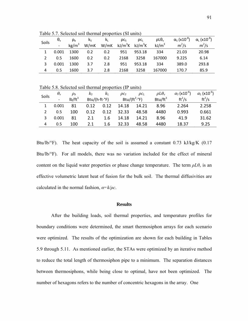
91

Btu/lb/°F). The heat capacity of the soil is assumed a constant 0.73 kJ/kg/K (0.17

Btu/lb/°F). For all models, there was no variation included for the effect of mineral

content on the liquid water properties or phase change temperature. The term ρLθv is an

effective volumetric latent heat of fusion for the bulk soil. The thermal diffusivities are

calculated in the normal fashion, α=k/ρc.

Results

After the building loads, soil thermal properties, and temperature profiles for

boundary conditions were determined, the smart thermosiphon arrays for each scenario

were optimized. The results of the optimization are shown for each building in Tables

5.9 through 5.11. As mentioned earlier, the STAs were optimized by an iterative method

to reduce the total length of thermosiphon pipe to a minimum. The separation distances

between thermosiphons, while being close to optimal, have not been optimized. The

number of hexagons refers to the number of concentric hexagons in the array. One

Table 5.7. Selected soil thermal properties (SI units)

Soils θv ρb kS kL ρcS ρcL ρLθv αS (x10-8) αL (x10-8)- kg/m3 W/mK W/mK kJ/m3K kJ/m3K kJ/m3 m2/s m2/s

1 0.001 1300 0.2 0.2 951 953.18 334 21.03 20.982 0.5 1600 0.2 0.2 2168 3258 167000 9.225 6.143 0.001 1300 3.7 2.8 951 953.18 334 389.0 293.84 0.5 1600 3.7 2.8 2168 3258 167000 170.7 85.9

Table 5.8. Selected soil thermal properties (IP units)

Soils θv ρb kS kL ρcS ρcL ρLθv αS (x10-6) αL (x10-6)- lb/ft3 Btu/(h·ft·°F) Btu/(ft3·°F) Btu/ft3 ft2/s ft2/s

1 0.001 81 0.12 0.12 14.18 14.21 8.96 2.264 2.258 2 0.5 100 0.12 0.12 32.33 48.58 4480 0.993 0.661 3 0.001 81 2.1 1.6 14.18 14.21 8.96 41.9 31.62 4 0.5 100 2.1 1.6 32.33 48.58 4480 18.37 9.25

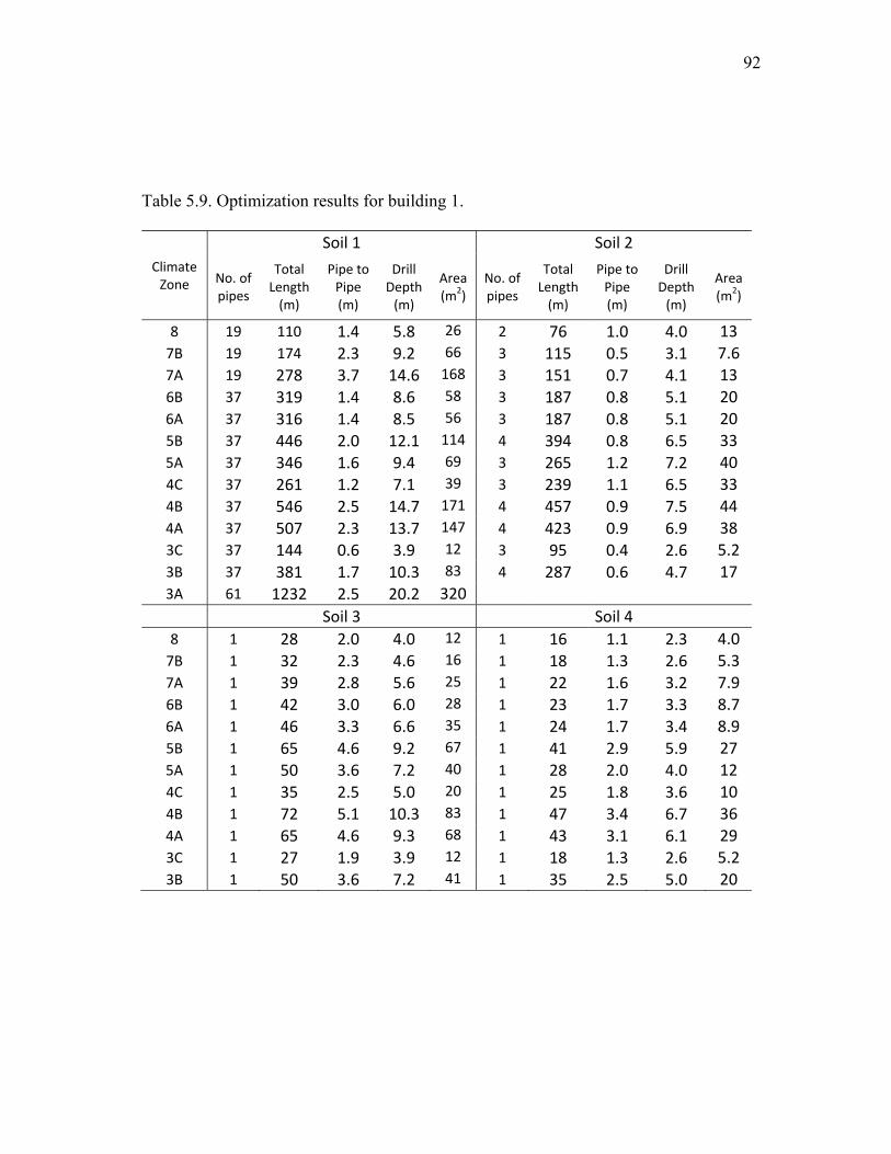
92

Table 5.9. Optimization results for building 1.

Climate Zone

Soil 1 Soil 2

No. of pipes

Total Length

(m)

Pipe to Pipe (m)

Drill Depth

(m)

Area (m2)

No. of pipes

Total Length

(m)

Pipe to Pipe (m)

Drill Depth

(m)

Area (m2)

8 19 110 1.4 5.8 26 2 76 1.0 4.0 13 7B 19 174 2.3 9.2 66 3 115 0.5 3.1 7.6 7A 19 278 3.7 14.6 168 3 151 0.7 4.1 13 6B 37 319 1.4 8.6 58 3 187 0.8 5.1 20 6A 37 316 1.4 8.5 56 3 187 0.8 5.1 20 5B 37 446 2.0 12.1 114 4 394 0.8 6.5 33 5A 37 346 1.6 9.4 69 3 265 1.2 7.2 40 4C 37 261 1.2 7.1 39 3 239 1.1 6.5 33 4B 37 546 2.5 14.7 171 4 457 0.9 7.5 44 4A 37 507 2.3 13.7 147 4 423 0.9 6.9 38 3C 37 144 0.6 3.9 12 3 95 0.4 2.6 5.2 3B 37 381 1.7 10.3 83 4 287 0.6 4.7 17 3A 61 1232 2.5 20.2 320

Soil 3 Soil 4 8 1 28 2.0 4.0 12 1 16 1.1 2.3 4.0

7B 1 32 2.3 4.6 16 1 18 1.3 2.6 5.3 7A 1 39 2.8 5.6 25 1 22 1.6 3.2 7.9 6B 1 42 3.0 6.0 28 1 23 1.7 3.3 8.7 6A 1 46 3.3 6.6 35 1 24 1.7 3.4 8.9 5B 1 65 4.6 9.2 67 1 41 2.9 5.9 27 5A 1 50 3.6 7.2 40 1 28 2.0 4.0 12 4C 1 35 2.5 5.0 20 1 25 1.8 3.6 10 4B 1 72 5.1 10.3 83 1 47 3.4 6.7 36 4A 1 65 4.6 9.3 68 1 43 3.1 6.1 29 3C 1 27 1.9 3.9 12 1 18 1.3 2.6 5.2 3B 1 50 3.6 7.2 41 1 35 2.5 5.0 20

93


Climate Zone

Soil 1 Soil 2

No. of pipes

Total Length

(m)

Pipe to Pipe (m)

Drill Depth

(m)

Area (m2)

No. of pipes

Total Length

(m)

Pipe to Pipe (m)

Drill Depth

(m)

Area (m2)

8 91 1175 1.3 13 131 5 841 0.9 9.2 67 7B 127 2261 1.5 18 249 7 1376 0.6 8.1 52 7A 127 2793 1.8 22 380 8 1933 0.6 8.9 62 6B 127 3565 2.3 28 619 9 2306 0.5 8.5 57 6A 127 3483 2.3 27 591 8 2139 0.6 9.9 76 5B 169 5352 2.3 32 788 8 4292 1.2 20 307 5A 169 4527 1.9 27 564 9 3161 0.6 12 107 4C 127 3555 2.3 28 615 11 2708 0.3 6.8 37 4B 217 6792 2.0 31 769 10 5921 0.9 18 251 4A 217 5944 1.7 27 589 8 4620 1.3 21 356 3C 127 1686 1.1 13 138 7 1413 0.6 8.4 55 3B 271 5169 1.1 19 286 10 3986 0.6 12 114

Soil 3 Soil 4 8 7 94 6.7 13 140 1 100 7.2 14 162

7B 19 276 3.6 15 166 2 208 2.7 11 94 7A 19 327 4.3 17 233 2 257 3.4 14 144 6B 19 365 4.8 19 290 2 279 3.7 15 170 6A 19 364 4.8 19 288 2 258 3.4 14 145 5B 19 567 7.5 30 699 3 528 2.4 14 160 5A 19 462 6.1 24 465 3 353 1.6 9.5 71 4C 19 428 5.6 23 399 2 319 4.2 17 222 4B 19 686 9.0 36 1025 3 729 3.3 20 305 4A 19 660 8.7 35 949 3 543 2.4 15 169 3C 19 239 3.1 13 125 2 168 2.2 8.8 61 3B 19 605 8.0 32 797 3 555 2.5 15 177

94


Climate Zone

Soil 1 Soil 2

No. of

pipes

Total Length

(m)

Pipe to

Pipe (m)

Drill Depth

(m)

Area (m2)

No. of

pipes

Total Length

(m)

Pipe to

Pipe (m)

Drill Depth

(m)

Area (m2)

8 631 28769 1.6 46 1633 14 20327 1.2 32 8157B 817 39794 1.5 49 1863 18 25333 0.7 25 4787A 1027 64197 1.7 63 3069 22 41250 0.6 27 5796B 919 63018 2.0 69 3693 19 41675 1.0 37 10486A 1027 76837 2.1 75 4396 20 47517 0.9 38 11155B 1027 89615 2.4 87 5980 21 69048 1.2 50 19465A 1141 100560 2.3 88 6101 21 69572 1.2 50 19764C 1141 80318 1.9 70 3892 22 72170 1.1 48 17734B 1141 104530 2.4 92 6591 21 83233 1.4 60 28284A 1519 131450 2.0 87 5881 24 94187 1.1 52 21483C 1657 77675 1.0 47 1726 24 53473 0.6 30 6923B 3571 218870 0.9 61 2950 35 153360 0.6 41 1292

Soil 3 Soil 4 8 61 2571 5.3 42 1395 61 2104 4.3 34 934

7B 91 4303 4.7 47 1756 169 3296 1.4 20 2997A 91 6272 6.9 69 3731 169 5236 2.2 31 7546B 91 6994 7.7 77 4639 169 4676 2.0 28 6016A 127 8231 5.4 65 3299 169 5586 2.4 33 8585B 127 9697 6.4 76 4579 169 8185 3.5 48 18425A 127 10218 6.7 80 5084 217 7168 2.1 33 8574C 127 9056 5.9 71 3993 217 9227 2.7 43 14204B 127 11140 7.3 88 6043 169 9523 4.0 56 24944A 169 14505 6.1 86 5786 217 11338 3.3 52 21443C 127 9646 6.3 76 4530 169 7564 3.2 45 15733B 271 26871 5.5 99 7721 331 22462 3.4 68 3617

95

hexagon refers to seven thermosiphon pipes with six forming a hexagon and one in the

center. Two hexagons indicates 19 thermosiphon pipes, three indicates 37 pipes, etc., as

shown in Fig. 5.1.

As to be expected, the number of hexagons, the total length of thermosiphon pipe,

and therefore the depth and the volume of the system all increase with building load and

warmer climates. The separation distance between thermosiphon pipes is primarily a

Figure 5.1. Number of pipes associated with 1, 2, and 3 hexagons.

96

function of soil thermal properties. In heat transfer applications, it is common for a

length parameter (l) in the problem to be proportional to the square root of thermal

diffusivity (α) multiplied by time (t),

∝ √ (5.8)

It was found that the average separation distance for each of the four soils across all three

buildings and all climate zones correlates to the square root of the thermal diffusivity of

the soil. This correlation is shown in Fig. 5.2, where the logarithm of thermal diffusivity

is plotted against the logarithm of the separation distance,

ln( ) ∝ 12 ln( ) + 12 ln( ) (5.9)

The error bars represent the population standard deviation from the mean. As long as the

time remains constant, the slope of the line should be ½ to indicate a correlation; from a

linear regression, the slope is found to be 0.45.

In every climate zone and every building, the total length of thermosiphon pipe

needed to handle the load decreases from soil 1 to soil 4. None of the soil thermal

properties in Table 5.7 (5.8) would indicate such a trend. However, the thermal

effusivity, e, which is a measure of a substance’s ability to exchange thermal energy with

its surroundings,

= (5.10)

was calculated for each of the soils. It was found that the thermal effusivity inversely

correlates to the length of pipe required. That is, as the thermal effusivity increases, the

ability to exchange heat is greater, and the length of pipe required to cool a load is

decreased. The thermal effusivities for the four soils are shown in Table 5.12.

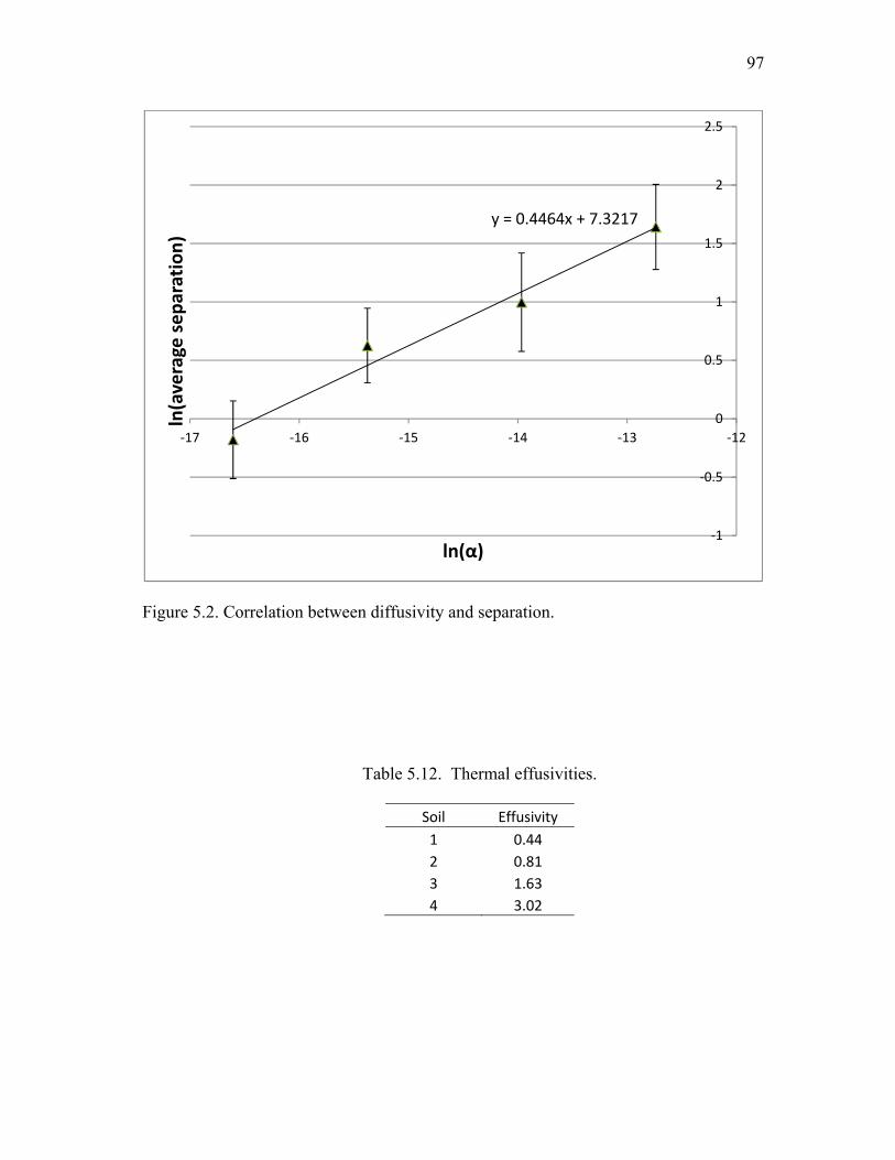
97

Figure 5.2. Correlation between diffusivity and separation.

Table 5.12. Thermal effusivities.

Soil Effusivity1 0.442 0.813 1.634 3.02

y = 0.4464x + 7.3217

-1

-0.5

0

0.5

1

1.5

2

2.5

-17 -16 -15 -14 -13 -12

ln(a

vera

ge se

para

tion)

ln(α)

98

Conclusion

Based on the validation of the modeling code and the results of the optimization,

the design methodology and code give a good idea as to the size and configuration of

smart thermosiphon arrays that are needed for a particular cooling load, in any climate,

and in any soil type. The correlation between pipe separation distance and thermal

diffusivity is robust and as expected from the similarity solutions shown in Appendix B.

In combination with the separation scaling to diffusivity, the trend relationship

between thermal effusivity and total pipe length could give a method to predict, a priori,

the optimal design of a thermosiphon array. These correlations also can lead to better

optimization and design methodologies.

In Tables 5.9 through 5.11, all 16 climate zones are not represented. The

optimization code was unable to find a viable solution in Dallas, Phoenix, Houston, and

Miami. This is a confirmation that smart thermosiphon arrays are difficult to implement

as standalone systems in locations with extremely hot climates, that rarely, or never,

experience freezing temperatures.

References

[1] ASHRAE, 2009, 2009 ASHRAE Handbook: Fundamentals, I-P Edition. American Society of Heating, Refrigerating and Air-Conditioning Engineers, Inc., Atlanta, GA, p. 14.1. [2] ASHRAE, 2007, ANSI/ASHRAE/IESNA Standard 90.1-2007, Energy Standard for Buildings Except Low-Rise Residential Buildings, American Society of Heating, Refrigerating and Air-Conditioning Engineers, Inc., Atlanta, GA, Appendix G [3] USGBC, 2009, LEED Reference Guide for Green Building Design and Construction, 2009 Edition, United States Green Building Council, Washington, D.C.

99

[4] ASHRAE, 2007, ANSI/ASHRAE/IESNA Standard 90.1-2007, Energy Standard for Buildings Except Low-Rise Residential Buildings, American Society of Heating, Refrigerating and Air-Conditioning Engineers, Inc., Atlanta, GA, Section 5.5. [5] ASHRAE, 2007, ANSI/ASHRAE/IESNA Standard 90.1-2007, Energy Standard for Buildings Except Low-Rise Residential Buildings, American Society of Heating, Refrigerating and Air-Conditioning Engineers, Inc., Atlanta, GA, Appendix B.

CHAPTER 6

CONCLUSIONS AND RECOMMENDED WORK

COMSOL Model

Instabilities in the COMSOL model led to the development of an original code in

MATLAB. It is presumed that the instabilities were caused by the discontinuities in the

thermal conductivity and specific heat at the phase change temperature. There are large

disturbances in the heat fluxes across the pipe wall in Fig. 2.9 at the time when freezing

begins to occur that clearly indicate freezing as a source of instability. However, there

are other smaller instabilities indicated by the spikes at other times in Fig. 2.9.

Instabilities arise in regions where the temperature has not dropped to the phase change

temperature. These instabilities could be explored further to understand the sensitivity to

discontinuities at the phase change.

It is possible that some of the instabilities are linked to the conditional statements

used to turn the boundary condition on and off depending on the outdoor air temperature

function. It is not entirely clear that the conditional statement comparing temperature in

the soil next to the pipe wall with the outdoor air temperature was performing as desired

and expected. Caution is advised when using conditional statements in COMSOL.

Further testing is warranted to confirm boundary condition was cycling as appropriate.

The temperature model, Eq. (2.7) removes extremes in the data. Removing

extremes causes the temperature difference between the ground and outdoor air

101

temperature to be muted. To a certain extent, it can be assumed that the amount of extra

cooling of the soil gained by the extreme cold temperatures would be balanced by the

heat added back by extreme hot temperatures during the summer season. However, it is

best if actual weather data can be modeled.

Although COMSOL was used to assist in the design of the pilot scale system, the

soil data used in the model was assumed without any testing or validation. The soil

thermal properties should have been measured beforehand and a model optimized for

spacing before the system was installed. Instead, the soil properties were partially

measured and estimated after gathering samples during the installation of the system. It

is highly recommended that soil properties are measured in situ prior to finalizing the

design. Because of the variation in soil lithography in the pilot scale and the lack of in

situ testing, it is unknown how close the pilot scale pipe spacing is to an optimized

design.

A more robust comparison of thermosiphon length with ground loop heat

exchanger (GLHE) length is needed. Soil variations can greatly affect the comparison.

The soil, weather, or building load differences may greatly affect the sizing of the GLHE,

making the comparison invalid. The comparison at the end of Chapter 2 is considered an

approximation only, and was not one of the stated purposes of this research.

COMSOL should have been used to optimize spacing in the hexagonal array.

This optimization would have been beneficial to make comparisons to the MATLAB

model. COMSOL was abandoned before the design criteria and constraints that went

into the MATLAB model were selected. Overall, COMSOL’s instabilities and

difficulties in modeling phase change make it impractical to use for the design and

102

optimization of thermosiphon arrays. However, the graphical interface and ability to

create and mesh 2-D and 3-D models easily give it an advantage over the MATLAB

code and could make it worthwhile to explore packaged software further.

Pilot Scale

The pilot scale was used as a brief demonstration of ground freezing using a

thermosiphon array. Before another system can be built of the same materials, the

wetting of R134a on the multiple interior surfaces of the thermosiphon needs to be tested

to identify the best materials for wetting, heat transfer, and cost. The mesh and inner

lining should be tested further to determine if heat transfer is truly enhanced by having

them installed.

The data acquisition system and the attached thermocouples did not function as

intended. Resistance based temperature measurements are recommended to achieve

results that are more precise.

The equipment used to control the thermosiphons should be custom manufactured

to meet the required specifications for submersion and insertion into a small diameter

pipe. The pump and float switch should be combined as one assembly with liquid tight

electrical connections, with separate power and signal wires.

Although the system was pressure tested at both positive and negative pressures,

five out of seven thermosiphon pipes would not hold their charge. Brazed fittings are

recommended for R134a systems. The heat exchangers should be brazed together instead

of soldered, and they should be structurally supported to withstand a high wind load.

103

To be experimentally valid, a control has to be used. It is recommended that a

thermosiphon array identical to the one tested is installed with no refrigerant, and also

monitored.

MATLAB Model

The thermal conductivity in the MATLAB model can be modeled either as a

sharp front, columnar, or using Kirchoff temperatures. That is, within the node where

phase change is occurring, it is considered to be occurring in series (sharp front), in

parallel (columnar), or isothermally (Kirchoff). These methods apply to pure phase

change materials (PCMs) only. Thermal conductivities for soils, which are porous

media, were considered in the model for frozen and unfrozen soils, but the effect porous

media has on slushy nodes was not examined. This effect should be studied and

incorporated into the model.

The solution for a moving front with a flux boundary showed a melt radius that

moves faster with a higher transcendental λt than the closed form solution when the melt

front is near the end of a node. This effect should decrease as the number of nodes is

increased, as was evidenced by the position of the melt front at the beginning of the

model where there are more nodes. However, it is unknown what was actually causing

this discrepancy from the closed form solution as the melt front approaches a nodal

boundary. It is suspected that the method of determining the location of the melt front

was at fault and not the model. The calculation of the melt front location did not

compensate for when there are two nodes at the melt temperature, which often happens as

the melt front is moving from one node to the next.

104

A hexagonal array was assumed to be the best for heat transfer because of close-

packing. However, a square array of thermosiphons may be better for ease of

installation. As part of a cost optimization and analysis, square arrays, and other more

readily installed patterns should be modeled.

The radius of the model should account for the area of the hexagon, not the area

of the circle inscribed in the hexagon, as shown in Eq. (3.34).

A conservative CFL stability criterion was used in the code to determine the

timestep, see Eq. (3.38). The stability criteria should be explored further. A test could be

included in the code to insure the freeze or melt front does not skip nodes or disappear

without meeting another phase change boundary.

The pressure and density were considered constant in the model. In reality,

pressure changes greatly with depth underground; therefore, so does the melt

temperature, the latent heat of fusion, and specific heat. Density changes with a phase

change and should be accounted for, especially in cases with high water content.

The PCM of interest, water, is always assumed to be pure. In reality, salts and

other chemicals in the soil will dissolve in the water and change the thermal properties of

the water, particularly the melt temperature and the heat of fusion. This should be

accounted for in the model to make a more robust design.

Design Optimization

The thermosiphons were modeled as if there is no thermal resistance from the

outdoor air to the wall of the thermosiphon pipe underground. There are thermal

resistances. With a good design, the thermal resistances are small. However, there is

opportunity to study the thermal losses and the variation of temperature with depth to

105

improve the design of the thermosiphon pipe itself. The losses for any particular

thermosiphon design should be quantified and included in the model.

Local building codes require economization when the outdoor air temperature is

below a specified shutoff limit. The shutoff limits vary between climate zones. The

economization was modeled in the optimization routine when the outdoor air temperature

is lower than the thermostat setting. The typical thermostat setting is not the code-

specified shutoff limit for all locations. There will also be times when the outdoor air

temperature is higher than the first node, but still below the shutoff limit. The changes in

the code that are required to model the shutoff temperature for a given location are easy

to make. As it is, the economization feature in the model can be improved.

There are other possibilities for pipe arrangement that might increase efficiency.

For example, a ring of thermosiphons without pumps on the outer edge of an array might

serve to reduce thermal losses to the surroundings, or the spacing might change from the

outer region to the inner region of the array. These possibilities cannot be modeled with

a one dimensional code. A two-dimensional or three-dimensional code would have to be

created to accommodate more complicated pipe arrangements.

The optimization routine did not find a solution for Dallas, Phoenix, Houston, or

Miami during the allotted time. This failure does not mean it cannot be done. It only

means the method used to search for a minimum did not converge.

A similar algorithm for optimization should be developed for pipe separation

distances. An optimization of pipe separation distances may show a better correlation

with soil thermal diffusivities. Diffusivity and separation correlate well, and with better

correlations, a separation could be determined without running a transient model, and

106

then the model could be used to minimize total length from the fixed separation. The

number of iterations performed to find an optimum would decrease and the speed of

optimization would be greatly increased.

Future Work

Even though the design discussed here only covers space cooling, a similar

analysis could be done for space heating, made slightly more complicated by increased

convection within the soil and solar radiation gains. The current cooling model could be

expanded to include three dimensions, including end effects, convection and solar

radiation surface gains. In addition, longer simulation times will need to be used to find

the long-term effects such a system might have on the local ecosystems. More prototypes

should be placed in the ground and monitored to gather experimental data. Work is

moving quickly toward several full-scale implementations.

The design and optimization study should be expanded to include the coupling of

heat pumps with thermosiphons. This combination opens the system to various

operational modes that would have to be modeled. This also opens the market of

thermosiphon arrays to hot climates where freezing temperatures do not typically occur.

Consideration of Possible Alternatives

Although more heat losses will occur, there is another possibility that would make

the system completely passive. The heat pipes can slant through the ground from the

back fence of the yard to the bottom of the basement where they combine and flow into a

heat exchanger that is inside a plenum with forced air. A valve is shut off just outside of

the foundation during the winter season. The ground freezes as the thermosiphons

107

operate as described previously. After the ground is frozen and the weather warms up,

the valves are opened when cooling is desired. Air is forced past the exchanger and the

thermosiphons continue to work in the same manner. As long as the location of the heat

sink is physically above the location of the heat source, no pumping is required. This

system would be completely passive, excluding the fan, and would be easily adapted to

existing thermostat control systems. No tank or flow divider is necessary. No drilling

would be necessary, which would bring down the cost. Further modeling needs to be

done to determine if the area is adequate, if the heat gains are acceptable, and to see if the

sprinkler system has a path where it won’t freeze year-round. This would be much easier

to implement if there were a naturally occurring slope, hill or mountainside, adjacent to

the building.

Final Conclusions

The design and optimization of smart thermosiphon arrays was a success. A

strong correlation was found between thermal diffusivities and thermosiphon pipe

separation distance. It was found that the separation is proportional to the square root of

the soil thermal diffusivity. An inverse correlation was found between total pipe length

and thermal effusivity. Viable design solutions were found through an iterative

optimization routine for three buildings in twelve locations and four different soil types.

More research in materials and manufacturing is needed for successful implementation of

working full-scale smart thermosiphon arrays.

APPENDIX A

DESIGN

This appendix describes the design of a sample smart thermosiphon array (STA)

cooling system for a 2,000 sq. ft. house in Midvale, UT. The design was partially

implemented as a pilot scale study described in Chapter 4. The same residence was used

as Building 1 in the design optimization software described in Chapter 5.

There were three objectives to the design of the cooling system. The first is rather

implied, but it is to meet the load requirements of the house in consideration. The second

design objective is for the system to consume the least possible amount of energy for

operation without sacrificing the third objective, which is to make it economically

attainable for the owner and for homeowners in general.

Load Calculation

To size the system, first a load calculation needed to be done for the house. This

load calculation took into consideration the conduction through the walls, the windows,

roof and floor. It also took into consideration solar heat gains, heat generation by

occupants and air infiltration. The load calculation was done to determine the maximum

load that the home would most likely see. This would be the maximum cooling the

system would need to provide during the hottest summer months. The load is based on a

summer temperature of 105ºF and a room temperature of 70ºF. This peak load, the

109

maximum rate of cooling, is how most air conditioning systems are designed. However,

with seasonal thermal energy storage, an integrated load, or the total amount of heat that

needs to be transferred over the course of the entire year, must be calculated. Due to the

lack of tools to perform this calculation, it is not done prior to the pilot scale

implementation. It is performed for the later optimization discussed in Chapter 5.

Thermosiphon Sizing and Determination

Thermosiphon modeling was completed in COMSOL 3.3, a complete description

of this can be found in CHAPTER 2. Several assumptions were made in these models

that are listed in the assumptions section below. The models took into consideration

conduction only. Heat transfer will be amplified in cases where convection occurs in the

soils [1]. Total heat flux was calculated for the heat pipes and integrated over the length

of the year to determine total amount of energy stored (or rather, removed) during the

winter months per length of heat pipe. The sizing of this system required a total

integrated energy load and a peak power load. Without a method to determine the load

profile and integrated load, an article by Jeff Spitler was used to correlate monthly peak

loads with integrated monthly loads [2].

Constraints of the System

1. The system must fit within the backyard of the home, which is approximately 30’x50’.

2. The heat exchange panels for the outdoors are designed to replace fencing and

therefore cannot be taller than 6 feet, or longer than the perimeter of the backyard, which

is taken to be 110 feet.

110

3. Any method of installation cannot involve equipment larger than a rig transported by a

single standard-size vehicle in order to gain access to the yard and cannot have a

clearance of over 12 feet because of overhead power lines.

4. Internal mechanical systems must fit within the infrastructure of the building.

5. Pipe diameters are to match nominal pipe sizes to minimize cost. The pump is sized

based on the cooling load.

6. The drilling method chosen, direct-punch, constrains the thermosiphon pipe diameter

to a maximum of 3”-nominal piping.

7. Availability of pumps that fit inside the thermosiphon pipe limit the internal diameter

to a minimum of 2”-nominal piping.

Assumptions

Load Calculation 1. The peak load to integrated load ratio is a constant. This implies that an integrated

load can be calculated by scaling from the known peak load and integrated loads of

another building. This is a weak assumption, especially when the building sizes, shapes,

and materials, are drastically different or when seasonal variations are different.

2. The building in Oklahoma and the house in Midvale have comparable seasonal

variations and are built in similar enough manners to warrant a direct comparison of

cooling loads. This is probably the weakest of all assumptions, but proves to be

adequate.

111

COMSOL Model

1. A thermosiphon spacing of 1.5 m is optimum. This spacing was found to be optimum

compared to two others: 0.5 m and 5 m. Further optimization using COMSOL was

considered to be cumbersome and was discontinued for this design, but subsequent

COMSOL modeling is included in Chapter 2. Additional optimization using MATLAB

code is described in Chapter 5.

2. In general, vapor-liquid equilibrium and all other thermodynamics were ignored.

Only latent heat and working pressure as a function of temperature were considered.

3. The soil modeled had the following characteristics:

a. The soil is completely saturated with pure water.

b. Soil porosity (φ ) is 35%.

c. Initial soil temperature is 285 K (53.3 Farenheit).

d. The thermal conductivity of the soil is given by an empirical function of

temperature (in S.I. units) developed from literature values, as in Eq. (2.2).

e. The density and heat capacity of the soil are given by Eq. (2.3) and Eq. (2.4),

where the density of water is 1000 kg/m3, and the density of soil is 2650 kg/m3. The heat

capacity of water is 4180 and soil is 1003 J/(kg K).

4. The thermosiphons only have heat transfer occurring during the winter if the

temperature of the ground next to the heat pipe is greater than the ambient temperature

outside.

5. The ambient temperature outside is given as a function of time that was fitted using

two sine curves to SLC International Airport weather station average temperatures. One

112

sine curve was used for 24-hour daily temperature oscillations and the other for yearly

seasonal oscillations.

6. Heat losses and gains to the surface were neglected, assuming that the thermosiphons

are deep enough for this to be true. All other end effects were neglected.

7. No convection occurs in the soil.

8. Only 85% of the heat transferred out of the soil can be transferred back into the soil

because the cooling front extends beyond the reach of recoverability for the heat pipes.

10. The optimal design for the thermosiphons is for the depth of the pipes to be the same

as the diameter of the pipe matrix. This is to reduce the surface area to volume ratio and

therefore minimize heat gains.

External Heat Exchangers

1. The fencing on the perimeter of the yard will be sufficient heat exchange area to

provide the cooling necessary.

2. Labor of installation and cost of fencing is considered as outside the scope of this

bid/estimate.

Other External Labor

1. It is assumed that any removal of old fencing, or trees, bushes, etc. will be done before

this project is initiated, and cost does not cover the preliminary work to prepare for the

system. This includes any light trenching, pole digging, sod and landscape preservation,

etc.

113

Internal Mechanical Systems

1. Ductwork, fans, plenum, and heating systems are all as-is, and any change or

modification that takes place to these systems is not part of this analysis.

2. Any control devices, such as thermostats, flow regulators/distributors, wiring, etc. are

not included in this design. The pumps in each of the thermosiphons are considered

control devices and are therefore not included. These pumps are small, high head, low

flow, and relatively inexpensive pumps.

3. A storage tank will most likely be needed for such a system, but this also falls outside

of the scope of this work since thermodynamics are not considered; therefore, volume of

liquid in a vapor-liquid equilibrium is not calculated.

4. The length of piping within the house is not significant to contribute to head loss.

Head loss is only estimated since it is a two phase system.

5. The correction factor for the cross-flow heat exchanger inside the house is 1.

Heat Load Calculation

The home was estimated to have an electrical load of approximately 1watt per

square foot of the home and approximately five occupants each giving off 450 Btu/hr.

Once all of the heat gains were calculated, the total required cooling load was

determined. The calculated max load for the home was 16.2 kW (55,140 BTU/hr, 4.6

tons of cooling).

Heat Pipe Field Design

The COMSOL model was integrated, and it was determined that each heat pipe

had a potential to remove 68 J/m of heat energy from the ground over the course of the

114

cold season. Based on the integrated heat load calculated by scaling the Oklahoma case,

this is equivalent to 120 m of total length. If the heat pipes are separated by 1.5 m each in

equilateral triangles, this is equivalent to 19 heat pipes, each 6 m deep.

Refrigerant Selection

Since the system operates on the principle of latent heat capture, refrigerants

releasing latent heat of vaporization at 25°C and those which are not freezing at 0°C are

employed. Considering the operating temperatures, the choice of refrigerants is narrowed

to R134a (tetrafluoroethane) and ammonia. The operating pressures for R134a and

ammonia are 3 bar and 5 bar, respectively. The latent heat of vaporization of R134a is

200 kJ/kg, and that of ammonia is 1,400 kJ/kg. Although ammonia facilitates better heat

transfer, R134a is chosen as ammonia is considered toxic and is difficult to manage at

that pressure. R-134a also offers the advantage of being commercially available without

a license requirement.

Cost Estimate

Collecting all the individual systems and totaling the cost gives a final result of

$4400 for drilling costs, $5890 for outdoor systems (excluding the fence), $1100 for

indoor systems, and an approximated 100 man-hours or $1000 of labor costs. The fence

heat exchangers are approximated to cost $5000 but need to be investigated further. The

total energy costs are the same as running an air conditioner minus the compressor

(which is the primary consumer in an A/C system). That brings the grand total to

$12,390 without the fence and $17,390 with the fence.

115

References

[1] Kekelia, B., 2012, “Heat Transfer To and From a Reversible Thermosiphon Placed in Porous Media,” Ph.D. dissertation, The University of Utah, Salt Lake City, UT. [2] Spitler, J.D., 2000, “GLHEPRO—A Design Tool For Commercial Building Ground Loop Heat Exchangers,” Proceedings of the Fourth International Heat Pumps in Cold Climates Conference, Aylmer, Quebec.

APPENDIX B

ANALYTICAL SOLUTIONS

When a thermal energy storage system contains a phase change material (PCM),

such as water, the latent heat of the material must be taken into consideration. The

mathematical modeling of phase change is considerably more complicated than simple

heat transfer, due to the nonlinearity of the system and the fact that one of the unknowns

is the location of the phase change boundary. A few analytical solutions exist, and one is

presented here as the basis of the simulation and design methodology presented in

Chapter 3.

Assumptions

Before any solutions are presented, a discussion of the assumptions included is

necessary. These assumptions are held throughout all methods, including the numerical

simulations in Chapter 3. They do not apply to the COMSOL modeling discussed in

Chapter 2.

For simplicity, heat is assumed to be transferred in the soil by isotropic

conduction only; radiation and convection are considered to have a negligible effect. All

other physical effects, such as gravitational, elastic, chemical, electromagnetic, and

nuclear, are ignored.

117

All thermal and physical properties are considered constant. That is, latent heat

(L) is constant and is released or absorbed at the melt temperature, which is also constant.

This assumption is probably valid for smaller systems, but pressure increases with depth

underground, and the melt temperature of water, the PCM of interest, decreases.

Therefore, this assumption comes in to question for a deeply installed system.

The densities of the liquid and solid phase are assumed to be equal (ρL=ρS). This

is necessary to avoid movement of the material, which complicates the mathematical

formulation of the problem. The heat capacity and thermal conductivity are only

assumed to be constant within a phase but differ between phases (cL≠cS, kL≠kS). Because

the temperature range of interest is relatively small, constant heat capacity and thermal

conductivity are reasonable. It is assumed there is no supercooling, and that there is a

sharp separation, with no thickness, between phases, at the melt temperature (Tm).

A pipe installed vertically in the ground is most readily modeled in a one-

dimensional radial geometry. Therefore, discussion is limited to cylindrical coordinates,

and the classical Stefan problem of phase change in a slab is not included.

The Stefan Formulation

The Stefan formulation [1] is concerned with the total energy (assuming no

kinetic or potential energy for the system) in a substance. Barring volume changes, for a

substance heated under constant pressure, the total energy is the internal energy of the

substance. The internal energy per unit mass is denoted by e, in kJ/kg, and the internal

energy per unit volume is denoted by E, in kJ/m3. The specific heat under constant

pressure is defined as the energy that is required to raise the temperature of 1 kg of a

substance by 1°C. That energy contained in a material is known as its sensible heat.

118

If the energy scale is determined by setting e=0 when the substance is a solid at its

melt temperature (Tm), and e=L when the substance is a liquid at the melt temperature,

the energy of the substance is given by

= ( ) = + [ − ], ≥( ) = [ − ], ≤ (B.1)

The heat flux ( ) is defined as the amount of heat energy crossing a unit area per unit

time. The heat flux is given by Fourier’s Law:

= − ∇ (B.2)

In one-dimensional cylindrical coordinates, Eq. (B.2) reduces to

= − (B.3)

With thermal diffusivity defined as = / , a heat balance, or energy

conservation, with the assumption that thermal conductivity and specific heat are constant

and no generation, leads to the heat equation:

= ∇ (B.4)

In one-dimensional cylindrical coordinates,

1 = + 1 (B.5)

In order to solve this parabolic differential equation, all boundaries must have a specified

boundary condition, and an initial temperature must be specified everywhere for t=0.

For a two-phase system, there exists an interface, assumed to be of zero thickness,

which separates the liquid from the solid. Within each phase, there is a distinct heat

equation satisfied with boundary conditions specified on the interface. The applicable

boundary condition is that of constant temperature. Where a phase change is occurring, it

119

is assumed that the temperature is the melt temperature, which is constant. The location

of the phase change boundary is unknown, but if it were known, there would be enough

information to solve for the temperature at all locations inside the liquid and solid

regions.

In order to locate the interface, a local heat balance can be derived for the

interface. The amount of energy released (or absorbed) per unit volume, during a phase

change, is given by

= ( − ) (B.6)

At the phase change boundary, = , and therefore, = . If an interface is moving

at some velocity ( ), the amount of energy released (or absorbed, depending on sign and

convention) per unit area of the interface will be . Therefore, the sum of the fluxes

normal to the interface must equal this generation,

= ( ∙ ) − ( ∙ ) (B.7)

Equation (B.6) is known as the Stefan Condition.

In one-dimensional cylindrical coordinates, the location (radius) of the interface,

as a function of time, can be denoted as R(t). Therefore, the interface velocity is

represented by the derivative with respect to time, R’(t). The flux normal to the interface

is given by Fourier’s Law, and the Stefan Condition for cylindrical coordinates in one-

dimension becomes

( ) = − ( ( ), ) + ( ( ), ) (B.8)

120

Applicable Problem

With the background of the Stefan Problem set up, it is now possible to show the

problem applicable to soil freezing, or melting, from an imposed flux at a thermosiphon

wall. Relatively few Stefan problems can be solved explicitly. Only two problems in

cylindrical coordinates have been found to have practical application. As with all closed-

form explicit solutions of Stefan problems, these two solutions are for a semi-infinite

domain, and therefore are similarity solutions [1]. Because of the nonlinearities inherent

in the problem of phase change, superposition is not a possibility. One of the solutions is

for the solidification of a supercooled melt. The other, shown here, is the solution for the

melting of an infinite solid from a line heat source of magnitude Q (W/m) at = 0. The

differential equation to be solved, Eq. (4.5), must be solved for both phases, namely

= + 1 , 0 < < ( ), > 0 ( ) (B.9)

= + 1 , ( ) < < ∞, > 0 ( ) (B.10)

With the interface conditions,

( ( ), ) = , > 0 (B.11)

( ) = − ( ( ), ) + ( ( ), ) , > 0 (B.12)

with initial conditions,

(0) = 0, ( , 0) = < (B.13)

and boundary conditions,

lim→ −2 = (B.14)

121

lim→ ( , ) = (B.15)

where Ts is the initial and far-field temperature of the solid.

The similarity solution for this problem is [2]

( ) = 2 , > 0 (B.16)

( , ) = + 4 4 − ( ) ,0 < ≤ ( ), > 0

(B.17)

( , ) = + ( − ) 4 , ≥ ( ), > 0 (B.18)

The variable is the root of

4 + ( − ) = (B.19)

where the function is the exponential integral [3]

( ) = , > 0 (B.20)

and s in Eq. (B.20) is a dummy variable for the purpose of integration.

Although this is an explicit closed-form solution for the problem as it was stated,

it is not congruent with real melting processes. The solution indicates that for any time > 0, the solid begins to melt, and the position of the interface is proportional to √ .

However, reality shows that if ≪ , there is a time elapsed to overcome the heat

capacity of the solid and increase its temperature at the boundary to before melting

occurs. The fact that line sources have some thickness can compensate for this error in

the solution but introduces error of its own.

122

References

[1] Alexiades, V., and Solomon, A.D., 1993, Mathematical Modeling of Melting and Freezing Processes, Hemisphere Publishing Corporation, pp. 117-120. [2] Carslaw, H., and Jaeger, J., 1959, Conduction of Heat in Solids, 2nd edition, Clarendon Press, Oxford. p. 294. [3] Abramowitz, M., and Stegun, I., 1965, Handbook of Mathematical Functions, Dover Publications, New York, NY.

APPENDIX C

SIMULATION CODE

As an example, the temperature boundary condition modeled in Chapter 3 is

performed by calling the code in Appendix B, from the matlab command line, with the

command: [r, deltat, deltar, T, E, unmet, economized]=cyl_exp_all_all(.0254, 0.25, 10, -

12, 1, 0.00058, 0.00218, 4000, 2000, 334000, 0, 1, 'hourlyload', 25, 31536000, 'Kir',

'temp');

The inputs, in order, are the inner and outer radius, in m, the number of radial

nodes (10), the initial temperature of the domain (-12°C), and the initial phase of the

PCM (1, indicating liquid), which is ignored when the initial temperature is not equal to

the melt temperature, which in this case is 0°C. The input parameters that follow are the

thermal properties of the material, which in this case match the thermal properties of

water. The last six inputs are the inner boundary temperature (1°C), a dummy variable

that does not apply to the ‘temp’ boundary condition, the outer boundary temperature

(25°C), the total simulation time in seconds (31536000 seconds = 1 year), the method of

calculating thermal conductivities (Kirchoff temperatures), and the boundary condition

type (‘temp’).

function [r, deltat, deltar, T, E, unmet, economized] = cyl_exp_all_all(Ri,Ro,rnodes,Tinit,lambdainit,kl,ks,rhoCl,rhoCs,rhoL,Tm,hourlytemps,hourlyload,Tstat,maxtime,con,boco) %% AMBI unmetcount=0; economized=0;

124

Tout=Tstat; Tin=hourlytemps; %% ALL time=0; %actual simulation time n=1; %time-step index for i=1:rnodes % Setting up the mesh r(i)=Ri+(sum(1:i-1)+i/2)/sum(1:rnodes)*(Ro-Ri); deltar(i)=i/sum(1:rnodes)*(Ro-Ri); end r(rnodes+1)=Ro; % Outer radius, last node deltat=min((min(deltar)^2)/(2.1*max(kl/(rhoCl),ks/(rhoCs))),3600); %fixes size of time step to deltay^2/(4*max alpha) twopi=6.28; % Shouldn't be necessary %% for node=1:rnodes T(node,1)=Tinit; %Initial temperature of domain if con=='Kir' R(node+1)=log(r(node+1)/r(node))/(twopi); %Resistance of the wall between node and node+1, check calculations but twopi should cancel out. end if T(node,1)<Tm %Initial energies and phases based on temperature E(node,1)=rhoCs*(T(node,1)-Tm); %frozen, below freezing, solid lambda(node,1)=0; elseif T(node,1)>Tm %melted, above freezing, liquid E(node,1)=rhoCl*(T(node,1)-Tm)+rhoL; lambda(node,1)=1; else %at freezing, user defined phase, slushy lambda(node,1)=lambdainit; E(node,1)=rhoCl*(T(node,1)-Tm)+rhoL*lambda(node,1); end end R(1)=log(r(1)/Ri)/(twopi); %Resistance from inner radius to first node R(rnodes+1)=log(Ro/r(rnodes))/(twopi); %% while time<maxtime %time limit of simulation in seconds %% %% AMBI if boco=='ambi' hour=floor(time/3600)+1; Tamb=hourlytemps(hour); qload=hourlyload(hour); %needs to be calculated per unit length!!!!!! end

125

%% DETERMINATION OF THERMAL CONDUCTIVITIES/KIRCHOFF TEMPERATURES %% ALL, ALL for node=1:rnodes if con=='col' k(node)=lambda(node,n)*kl+(1-lambda(node,n))*ks; else k(node)=1/(lambda(node,n)/kl+(1-lambda(node,n))/ks); end if T(node,n) < Tm %solid u(node)=ks*(T(node,n)-Tm); elseif T(node,n) > Tm %liquid u(node)=kl*(T(node,n)-Tm); else %slushy u(node)=0; end end %% CALCULATION OF FLUXES FOR ALL INTERIOR NODES % KIR if con=='Kir' for wall=2:rnodes %calc of fluxes q(wall,n)=(u(wall-1)-u(wall))/R(wall); end else % COL/SHF for wall=2:rnodes %calc of resistances and fluxes R(wall)=log(1+0.5*deltar(wall-1)/r(wall-1))/(2*pi*k(wall-1))-log(1-0.5*deltar(wall)/r(wall))/(2*pi*k(wall)); q(wall,n)=(T(wall-1,n)-T(wall,n))/R(wall); end end %% CALCULATION OF FLUXES FOR OUTER BOUNDARY NODE % ALL, TEMP if boco=='temp' q(rnodes+1,n)=k(rnodes)*(T(rnodes,n)-Tout)/R(rnodes+1); else % ALL, FLUX/AMBI q(rnodes+1,n)=0; end %% CALCULATION OF FLUXES FOR INNER BOUNDARY NODE % ALL, AMBI if boco=='ambi' if Tamb>T(1,n) & qload~=0 %Outside air temperature is higher than first node & there is a building load Tret=qload*R(1)/k(1)+T(1,n); %Tret is the temperature that would need to be returned from the conditioned space to satisfy the load if Tret>Tstat %If Tret is greater than the thermostat setting,

126

Tret=Tstat; %the maximum return would be just over Tstat setting. unmetcount=unmetcount+1;%count it as a timestep where load was unmet end q(1,n)=k(1)*(Tret-T(1,n))/R(1); %put load in system elseif Tamb>T(1,n) & qload==0 %Outside air is greater than first node, but no building load q(1,n)=0; %No cooling or heating of system else %Otherwise OA temp will be lower than first node q(1,n)=k(1)*(Tamb-T(1,n))/R(1); %In which case, cool the system economized=economized+qload*deltat; %And economize any load that might exist. end %This economization is idealized, first node will never be above Tstat, but could be close, %so OA temp could be close to Tstat setting, requiring a large %airflow to truly economize. end % ALL, FLUX if boco=='flux' q(1,n)=-0.7512; %Flux needed to freeze pure water with Ro=0.25, Ri=0.0254 in ONE HOUR? end % ALL, TEMP if boco=='temp' q(1,n)=k(1)*(Tin-T(1,n))/R(1); end % ALL, ALL for node=1:rnodes E(node,n+1)=E(node,n)+deltat/(deltar(node)*twopi*r(node))*(q(node,n)-q(node+1,n)); %Calculate new energy for all nodes if E(node,n+1)<=0 %solid T(node,n+1)=Tm+E(node,n+1)/rhoCs; %new temp lambda(node,n+1)=0; %new phase elseif E(node,n+1)>=rhoL %liquid T(node,n+1)=Tm+(E(node,n+1)-rhoL)/rhoCl; lambda(node,n+1)=1; else %slushy T(node,n+1)=Tm; lambda(node,n+1)=E(node,n+1)/rhoL; end end %% DISPLAY OPTIONS % q=[q(:,n)] time % day=hour/24 lET=[lambda(:,n),E(:,n)*10^-5,T(:,n)] if sum(E(:,n+1))<0 break

127

end %% % for node=1:rnodes % if T(node,n)==Tm % MeltR(n)=r(node)+(lambda(node,n)-0.5)*deltar; % % lamb(n)=MeltR(n)/(2*sqrt(kl/(rho*Cl)*time)); % % [n/1000,MeltR(n),lamb(n)] % end % end %% n=n+1; %Increase time-step time=time+deltat; %Calculate new actual time end unmet=unmetcount*deltat/3600; %Total unmet hours

APPENDIX D

OPTIMIZATION CODE

designoptimizer.m

clear all; clc; dlmwrite('logfile.txt',8.23,'-append'); starthour=6900; %hour of the year simulation starts maxtime=8760*3600; %amount of time simulation runs in seconds maxhours=ceil(maxtime/3600); %amount of time simulation runs in hours newyears=floor((starthour+maxhours)/8760); %number of times weather file needs to be cycled to the beginning TstatF=75; Tstat=(TstatF-32)*5/9; Tm=0; %Melt temperature of substance in deg celsius L=334; %Latent heat of fusion (kJ/kg) Ri=0.0254; %radius of thermosiphon pipe for zone=4 %% READ LOAD AND TEMPERATURE DATA zonestr=int2str(zone); tmyfile=strcat('weather',zonestr,'.xls'); tmy=xlsread(tmyfile, 'AF3:AF8762'); %tmy weather file gets read in as tmy, 8760 hourly temperature data points loadfile=strcat('load',zonestr,'.xls'); Tinit=mean(tmy); %initial temperature of domain, should be average of yearly temperatures for any location. for building=1 buildingstr=int2str(building); if building==1 range='E4:E8763'; elseif building==2 range='F4:F8763'; else range='G4:G8763'; end load=xlsread(loadfile,range)*3.51685; %hourly load profile from trane trace (converted from tons to kilowatts). unmetmax=max(size(nonzeros(load))); count=0; %variable counting how many years of data have been added to the hourly temperature vector

129

hourlytemps=tmy(starthour:8760); %hourly temperature vector starting at start hour and ending at the last hour of tmy file hourlyload=load(starthour:8760); while count<newyears %loop to add additional years needed to cover the simulation length. hourlytemps=[hourlytemps;tmy]; %vertical concatenation of additional years to hourly temp vector hourlyload=[hourlyload;load]; count=count+1; %counter increase end for soil=2:4 zone,building,soil soilstr=int2str(soil); dlmwrite('logfile.txt',zone, '-append'); dlmwrite('logfile.txt',building, '-append'); dlmwrite('logfile.txt',soil, '-append'); %% ASSIGN THERMAL PROPERTIES OF SYSTEM if soil==1 thetav=0.001; rhob=1300; ks=0.0002; %Conductivity of solid (kW/mK) kl=0.0002; %conductivity of liquid (kW/mK) rhoCs=2*thetav*1000+0.73*rhob; rhoCl=4.18*thetav*1000+0.73*rhob; rhoL=1000*L*thetav; elseif soil==2 thetav=0.5; rhob=1600; ks=0.0002; %Conductivity of solid (kW/mK) kl=0.0002; %conductivity of liquid (kW/mK) rhoCs=2*thetav*1000+0.73*rhob; rhoCl=4.18*thetav*1000+0.73*rhob; rhoL=1000*L*thetav; elseif soil==3 thetav=0.001; rhob=1300; ks=0.0037; %Conductivity of solid (kW/mK) kl=0.0028; %conductivity of liquid (kW/mK) rhoCs=2*thetav*1000+0.73*rhob; rhoCl=4.18*thetav*1000+0.73*rhob; rhoL=1000*L*thetav; elseif soil==4 thetav=0.5; rhob=1600; ks=0.0037; %Conductivity of solid (kW/mK) kl=0.0028; %conductivity of liquid (kW/mK) rhoCs=2*thetav*1000+0.73*rhob; rhoCl=4.18*thetav*1000+0.73*rhob; rhoL=1000*L*thetav; end alphas=ks/rhoCs; alphal=kl/rhoCl; dlmwrite('logfile.txt', [alphas,alphal], '-append'); %% GEOMETRIC SETUP if min(tmy)<0 Emin=rhoCs*(min(tmy)-Tm);

130

else Emin=rhoCl*(min(tmy)-Tm)+rhoL; end if max(tmy)<0 Emax=rhoCs*(max(tmy)-Tm); else Emax=rhoCl*(max(tmy)-Tm)+rhoL; end deltaE=Emax-Emin; clear volume length T E unmetmatrix; %% OPTIMIZATION ENGINE for n=1:30; nstr=int2str(n); volume(n,1)=sum(load)*3600/deltaE; pipes=1+sum(6*(1:n)); count=1; unmet=1; while unmet>0 d=(4/3.14*volume(n,count))^(1/3); separation=d/(2*n); %distance between thermosiphons in meters Ro=separation/2; %radius of domain length(n,count)=(1+sum(6*(1:n)))*d; lengthstr=int2str(length(n,count)); loadperlength=hourlyload/length(n,count); rnodes=3; [r, deltat, deltar, T, E, unmet, economized]=meshtest(Ri,Ro,rnodes,Tinit,kl,ks,rhoCl,rhoCs,rhoL,Tm,hourlytemps,loadperlength,Tstat,maxtime); unmetmatrix(n,count)=unmet; unmetstr=int2str(unmet); deltatstr=int2str(deltat); econstr=int2str(economized); sepstr=num2str(separation); dlmwrite('logfile.txt',[n,length(n,count),separation,unmet,economized,deltat], '-append'); if unmet<88 break; end if (count > 2) & ((unmet==unmetmatrix(n,count-2)) | ((unmet>unmetmatrix(n,count-2)) & (unmet>unmetmatrix(n,count-1)))) break; end if count==2 lengthint=length(n,count-1)-unmetmatrix(n,count-1)*(length(n,count)-length(n,count-1))/(unmetmatrix(n,count)-unmetmatrix(n,count-1)); dint=lengthint/(1+sum(6*(1:n))); volume(n,count+1)=3.14*dint^3/4; else volume(n,count+1)=volume(n,count)*(1.05+5*unmet/unmetmax); end count=count+1; end

131

lengthtest=(1+sum(6*(1:n+1)))*(4/3.14*volume(n,1))^(1/3); if lengthtest>length(n,count) break; end end %% OUTPUTS % outfile=strcat('zone',zonestr,'results.xls'); % sheet=strcat('building',buildingstr,'soil',soilstr); % xlswrite(outfile,separation,sheet,'A1'); % xlswrite(outfile,length,sheet,'A2'); % xlswrite(outfile,unmetmatrix,sheet,'A22'); % xlswrite(outfile,r,sheet,'E1'); % xlswrite(outfile,deltat,sheet,'B1'); % xlswrite(outfile,economized,sheet,'C1'); % xlswrite(outfile,T',sheet,'A42'); %d=(4/3.14*volume(n,count))^(1/3); %separation=d/(2*n); %distance between thermosiphons in meters %Ro=separation/2; %radius of domain % disp('Press any key') % pause; end end end

meshtest.m

function [r, deltat, deltar, T, E, unmet, economized] = meshtest(Ri,Ro,rnodes,Tinit,kl,ks,rhoCl,rhoCs,rhoL,Tm,hourlytemps,hourlyload,Tstat,maxtime) unmetcount=0; time=0; %actual simulation time n=1; %time index economized=0; for i=1:rnodes r(i)=Ri+(sum(1:i-1)+i/2)/sum(1:rnodes)*(Ro-Ri); deltar(i)=i/sum(1:rnodes)*(Ro-Ri); end r(rnodes+1)=Ro; deltat=min((min(deltar)^2)/(2.1*max(kl/(rhoCl),ks/(rhoCs))),3600); %fixes size of time step to deltay^2/(4*max alpha) twopi=6.28; %Evar=deltat/(deltar*twopi); %%

132

for node=1:rnodes T(node,1)=Tinit; %Initial temperature of domain lambda(node,1)=1; R(node+1)=log(r(node+1)/r(node))/(twopi); if T(node,1)<Tm E(node,1)=rhoCs*(T(node,1)-Tm); else E(node,1)=rhoCl*(T(node,1)-Tm)+rhoL*lambda(node,1); end end R(1)=log(r(1)/Ri)/(twopi); %% while time<maxtime %time limit of simulation in seconds %% hour=floor(time/3600)+1; Tamb=hourlytemps(hour); qload=hourlyload(hour); %needs to be calculated per unit length!!!!!! for node=1:rnodes if T(node,n) < Tm %solid u(node)=ks*(T(node,n)-Tm); elseif T(node,n) > Tm %liquid u(node)=kl*(T(node,n)-Tm); else %mushy u(node)=0; end end %% for wall=2:rnodes %calc of fluxes q(wall,n)=(u(wall-1)-u(wall))/R(wall); end % R(rnodes+1,n)=log(Ro/r(rnodes))/(2*pi*k(rnodes)); % q(rnodes+1,n)=(T(rnodes,n)-Tout)/R(rnodes+1,n); q(rnodes+1,n)=0; k=1/(lambda(1,n)/kl+(1-lambda(1,n))/ks); if Tamb>T(1,n) & qload~=0 Tret=qload*R(1)/k+T(1,n); if Tret>Tstat Tret=Tstat; unmetcount=unmetcount+1; end q(1,n)=k*(Tret-T(1,n))/R(1); elseif Tamb>T(1,n) & qload==0 q(1,n)=0; else q(1,n)=k*(Tamb-T(1,n))/R(1); if Tamb<Tstat economized=economized+1; end end % q(1,n)=-0.0082967;

133

%% for node=1:rnodes E(node,n+1)=E(node,n)+deltat/(deltar(node)*twopi*r(node))*(q(node,n)-q(node+1,n)); if E(node,n+1)<=0 T(node,n+1)=Tm+E(node,n+1)/rhoCs; lambda(node,n+1)=0; elseif E(node,n+1)>=rhoL T(node,n+1)=Tm+(E(node,n+1)-rhoL)/rhoCl; lambda(node,n+1)=1; else T(node,n+1)=Tm; lambda(node,n+1)=E(node,n+1)/rhoL; end end % q=[q(:,n)] % time % day=hour/24 % lET=[lambda(:,n),E(:,n)*10^-5,T(:,n)] % if sum(E(:,n+1))<0 % break % end %% % for node=1:rnodes % if T(node,n)==Tm % MeltR(n)=r(node)+(lambda(node,n)-0.5)*deltar; % % lamb(n)=MeltR(n)/(2*sqrt(kl/(rho*Cl)*time)); % % [n/1000,MeltR(n),lamb(n)] % end % end %% n=n+1; time=time+deltat; end unmet=unmetcount*deltat/3600; economized=economized*deltat/3600;

SEASONAL UNDERGROUND THERMAL ENERGY STORAGE USING …

Documents

Transcript of SEASONAL UNDERGROUND THERMAL ENERGY STORAGE USING …